
NASA CR-54836
TRW ER-6673A
FINAL REPORT
THREE-DIMENSIONAL ANALYSIS
OF
INDUCER FLUID FLOW
By
PAUL COOPER and HEINRICH B. BOSCH
Prepared for
NATIONAL AERONAUTICS AND SPACE ADMINISTRATION
FEBRUARY I1, 1966
Contract NAS 3-2573
Technical Management
NASA Lewis Research Center
Cleveland, Ohio
Liquid Rocket Technology Branch
Werner R. Britsch
TRW AccEssOelesDIVISIONTRW INCt • 2355._ EUCLID AVENUE
CLEVELAND, r'lHIn 44117
https://ntrs.nasa.gov/search.jsp?R=19660012977 2018-06-12T02:26:37+00:00Z

_ r _

ABSTRACTAnalytical studies were conducted to provide means for improving
the design of inducers for high-speed, high-flow rocket engine pumps.
Exact and approximate methods are presented for obtaining three-
dimensional solutions to turbomachine flows with losses and vapori-
zation, and results are presented for two sample inducers. The exact
method solves four non-linear differential equations of motion simul-
taneously by finite-difference and relaxation techniques that employ
a "total residual 'r concept. Conclusions on inducer performance and
design are made on the basis of several approximate solutions of both
incompressible and two-phase flows, together with analysis of fluid
thermal and scale effects. Fortran IV listings of the analysis com-
puter programs are presented. _,_
J
ii


AC KNOW LE DGM ENTS
Special recognition for their regular consultation throughout the two-year
program covered by this report belongs to the following members of the
Fluid Systems Components Division at NASA Lewis Research Center under
the direction of Melvin J. Hartmann:
Donald M. Sandercock
James E. Crouse
Genevieve R. Miller
Dr. John D. Stanitz of TRW Inc. assisted in an advisory and review capa-
city, contributing much of his time to the effort. Credit goes to Professor
Howard W. Emmons of Harvard University and Professor Isaac Greber of
Case Institute of Technology for ideas which they contributed in the early
stages of the program.
.°°111


TABLE OF CONTENTS
ABSTRACT. ..............................
SUMMARY ....................... . ......
INTRODUCTION ............................
LIST OF SYMBOLS ...........................
I. FLUID FLOW RELATIONS ..................
A. The Flow Model .....................
1. Equations of Motion .................2. Relations for Two-Phase Flow and Loss Effects .....
B. Boundary Conditions ................. . .
1 Wall Boundaries
2. Throughflow Boundaries . . . . ............
II. THREE-DIMENSIONAL SOLUTION (EXACT METHOD) ......
A. Method of Solution .....................
1. Scalar and Finite'Difference Form of Basic Flow
Equations
2. Special Considerations at Boundary Points ........
3. Computational Algorithm Using Star Residuals ......
4. Accuracy Criterion ..................
5. Effects of Grid Point Density ..............6. Form of the Results ........ _.... ......
III.
B. Applications and Results ..................
1. Paddle-Wheel Channel with Wheel-Type Flow ......2. Paddle-Wheel Channel with Irrotational Flow ......
3. Three-Bladed, Variable-Lead Inducer Channels .....
C. Concluding Remarks on Exact Method of Solution .......
1. Review of Problems Solved ..............
2. Recommendations for Future Work ...........
APPROXIMATETHREE-DIMENSIONAL SOLUTION .......
A. Method of Solution ....................
1. Restrictions of the Analysis ............ . .
2. Scalar Equations and Boundary Conditions ........
ii
1
2
4
i0
10
10
12
15
15
I8
20
2O
20
25
27
29
32
35
36
38
42
51
78
78
79
81
81
81
84
iv

IV.
TABLE OF CONTENTS (Con't.)
3. Meriodional Streamline Balancing Procedure .......
4. Blade-to-Blade Solution ...............
5. Form of the Results ..................
B* Examples and Results ...................
1. Incompressible Results and Correlations for
Lossless Flow .....................
2. Effects of Two-Phase Flow and Losses ..........
C. Concluding Remarks About the Approximate Method of
Solution ..........................
INFLUENCE OF FLUID PHENOMENA ON THE PERFORMANCE AND
DESIGN OF INDUCERS .....................
A_ Characteristics of Equilibrium Two-Phase Flow and Loss
Model ..........................
1. Two-Phase Flow at Inducer Inlet ............
2. Discussion of Losses ..................
B. Performance and Scale Effects With Two-Phase Flow .....
1. Low-NPSH Tests of Inducers by the Analytical
Program .......................
2. Theory of Fluid and Scale Effects ............
3. Analysis of Results ....... ; ..........
C. Optimization of Geometry ..................
C ONC LUSIONS .......................
APPENDIXES ........................
A. Transformation from Cylindrical to General, Oblique
Coordinates ......................
B. Complementary Stream Functions ............
C. Instructions for Use of Exact Solution Computer
Programs .......................
D. Instructions for Use of Approximate Solution
Computer Programs ..................
REFERENCES ........................
DISTRIBUTION LIST ......................
89
93
96
96
101
123
125
125
125
129
132
132
135
141
143
147
149
149
155
161
187
213
V

FIGURE
SECTION I
I.l
1.2
SECTION II
II.1
II. 2
II.3
II. 4
II. 5
II. 6
II. 7
II. 8
II. 9
II.10
II.11
LIST OF FIGURES
PAGE
TYPICAL FLOW BOUNDARIES, INCLUDING UPSTREAMAND DOWNSTREAM FLOW REGIONS ............ 11
RELATIVE EDDY-FLOW AT TYPICAL INDUCER CROSS
SE C TION ......................... 17
ROTATING COORDINATE SYSTEM AND RELATIVE BASE
VECTORS ......................... 21
TYPICAL "STAR" OF GRID POINTS FOR FINITE-DIFFER-
ENCE EQUATIONS IN (a) CYLINDRICAL OR (b) GENERALCOORDINATE SYSTEMS .................. 23
COMPARISON OF METHOD OF SUCCESSIVE VARIATIONS
AND GRADIENT METHOD ................. 30
EFFECT OF GRID POINT DENSITY ............. 34
PADDLE-WHEEL CHANNEL FOR WHEEL.TYPE, AXIAL
FLOW CALCULATIONS .................. 39
INCOMPRESSIBLE, LOSSLESS, WHEEL-TYPE FLOW ..... 43
TWO-PHASE, LOSSLESS, WHEEL-TYPE FLOW ....... 44
PADDLE-WHEEL CHANNEL FOR IRROTATIONAL, AXIAL
FLOW CALCULATIONS .................. 45
DEMONSTRATION OF THE "TAKE-UP EFFECT" WITH
INCOMPRESSIBLE, IRROTATIONAL FLOW ......... 48
VELOCITIES IN INCOMPRESSIBLE, IRROTATIONAL FLOW 49
INFLUENCE OF THE TAKE-UP EFFECT AND GRID DENSITY
ON ATTAINABLE ACCURACY ............... 52
vi

FIGURE
II. 12
II. 13
II. 14
II. 15
II. 16
tI. 17
II. 18
II. 19
II. 20
II. 21
II. 22
II. 23
II. 24
LIST OF FIGURES (Continued)
PAGE
VARIABLE-LEAD INDUCER GEOMETRY FOR 6.2 ° BLADE
TIP INLET ANGLE ..................... 53
RESIDUAL RELAXATION DATA FOR INCOMPRESSIBLE,
LOSSLESS FLOW IN 6.2 ° INDUCER. . . . .......... 56
RADIAL DISTRIBUTIONS OF OUTLET VELOCITY AND
PRESSURE FOR INCOMPRESSIBLE, LOSSLESS FLOW
IN 6.2 ° INDUCER ..................... 57
OVERALL PERFORMANCE RELAXATION DATA FOR
INCOMPRESSIBLE, LOSSLESS FLOW IN 6.2 ° INDUCER .... 58
AXIAL DISTRIBUTIONS OF BLADE SURFACE PRESSURE
FOR INCOMPRESSIBLE, LOSSLESS FLOW IN 6.2 ° INDUCER . 59
AXIAL DISTRIBUTION OF BLADE SURFACE VELOCITY
FOR INCOMPRESSIBLE LOSSLESS FLOW IN 6.2 ° INDUCER . 6O
VARIABLE-LEAD INDUCER GEOMETRY FOR 12 ° BLADE
TIP INLET ANGLE .................... 62
RELAXATION DATA FOR INCOMPRESSIBLE, LOSSLESS
FLOW IN 12 ° INDUCER ................... 64
CIRCULATION RELAXATION DATA AT EXIT FOR
INCOMPRESSIBLE, LOSSLESS FLOW IN 12 ° INDUCER ..... 65
OVERALL PERFORMANCE RELAXATION DATA FOR
INCOMPRESSIBLE, LOSSLESS FLOW IN 12 ° INDUCER ..... 66
RADIAL DISTRIBUTIONS OF OUTLET VELOCITY AND
PRESSURE FOR INCOMPRESSIBLE, LOSSLESS FLOW IN
12 ° INDUCER. FREE PRESSURES .............. 67
RADIAL DISTRIBUTIONS OF OUTLET VELOCITY AND
PRESSURE FOR INCOMPRESSIBLE, LOSSLESS FLOW IN12 ° INDUCER: FORCED PRESSURES ............. 69
AXIAL DISTRIBUTIONS OF BLADE SURFACE VELOCITY FOR
INCOMPRESSIBLE, LOSSLESS FLOW IN 12 ° INDUCER: FREE
PRESSURES ........................ 71
vii
• _ j,°
FIGL_IE
II.25
II.26
II. 27
II. 28
II. 29
LIST OF FIGURES (Continued)
PAGE
AXIAL DISTRIBUTIONS OF BLADE SURFACE VELOCITY
FOR INCOMPRESSIBLE, LOSSLESS FLOW IN 12 °
INDUCER: FORCED PRESSURES ............... 72
AXIAL DISTRIBUTION OF BLADE SURFACE PRESSURE
FOR INCOMPRESSIBLE, LOSSLESS FLOW IN 12 °
INDUCER: FREE PRESSURES ................ 73
AXIAL DISTRIBUTIONS OF BLADE SURFACE PRESSURES
FOR INCOMPRESSIBLE, LOSSLESS FLOW IN 12 °
INDUCER: FORCED PRESSURES .............. 74
AXIAL DISTRIBUTIONS OF BLADE SURFACE VELOCITY
FOR TWO-PHASE, LOSSLESS FLOW IN 12 ° INDUCER ..... 75
AXIAL DISTRIBUTIONS OF BLADE SURFACE PRESSURE
FOR TWO-PHASE, LOSSLESS FLOW IN 12 ° INDUCER ..... 77
SECTION III
III. 1
III. 2
Ill. 3
III. 4
III.5
III. 6
TYPICAL FLOW FIELD FOR APPROXIMATE METHOD
OF SOLUTION ....................... 82
BLADE-TO-BLADE FLOW ANALYSIS, SHOWING RELATIVE
VELOCITY FIELD IN AN ANNULUS ............. 83
BLADE-TO-BLADE DISTRIBUTIONS OF FLUID FLOW
VARIABLES ........................ 92
ITERATIVE METHOD OF OBTAINING BLADE-TO-BLADE
SOLUTION FOR TWO-PHASE FLOW ............ 94
RADIAL DISTRIBUTION OF OUTLET VELOCITY AND
PRESSURE FOR INCOMPRESSIBLE, LOSSLESS FLOW
IN 6.2 ° INDUCER ...................... 99
RADIAL DISTRIBUTIONS OF OUTLET VELOCITY AND
PRESSURE AT BLADE TRAILING EDGE FOR INCOMPRESSIBLE
LOSSLESS FLOW IN 12 ° INDUCER, SHOWING CORRELATION
WITH EXACT METHOD ................... 100
,,.
Vlll

FIGURE
IH. 7
III. 8
III. 9
III. 10
IH. Ii
HI. 12
HI. 13
III. 14
III. 15
III. 16
LIST OF FIGURES (Continued)
PAGE
AXIAL DISTRIBUTIONS OF BLADE SURFACE VELOCITY
FOR INCOMPRESSIBLE, LOSSLESS FLOW IN 6.2 ° INDUCER . . 102
AXIAL DISTRIBUTIONS OF BLADE SURFACE PRESSURE FOR
INCOMPRESSIBLE, LOSSLESS FLOW IN 6.2 ° INDUCER .... 103
AXIAL DISTRIBUTIONS OF BLADE SURFACE VELOCITY
FOR INCOMPRESSIBLE, LOSSLESS FLOW IN 12 ° INDUCER,SHOWING CORRELATION WITH EXACT METHOD FREE
PRESSURE RESULTS .................... 104
AXIAL DISTRIBUTIONS OF BLADE SURFACE VELOCITY
FOR INCOMPRESSIBLE, LOSSLESS FLOW IN 12 ° INDUCER,SHOWING CORRELATION WITH EXACT METHOD FORCED
PRESSURE RESULTS .................... 105
AXIAL DISTRIBUTIONS OF BLADE SURFACE PRESSURE
FOR INCOMPRESSIBLE, LOSSLESS FLOW IN 12 ° INDUCER,SHOWING CORRELATION WITH EXACT METHOD FREE
PRESSURE RESULTS .................... 106
AXIAL DISTRIBUTIONS OF BLADE SURFACE PRESSURE
FOR INCOMPRESSIBLE LOSSLESS FLOW IN 12 ° INDUCER,SHOWING CORRELATION WITH EXACT METHOD FORCED
PRESSURE RESULTS .................... 107
BLADE-TO-BLADE DISTRIBUTIONS OF PRESSURE AND
RELATIVE VELOCITY, SHOWING COMPARISON OF EXACT
AND APPROXIMATE METHODS .............. 108
EFFECT OF LOSSES ON DISTRIBUTIONS OF OUTLET
VELOCITY AND PRESSURE FOR INCOMPRESSIBLE FLOW
IN 6.2 ° INDUCER ..................... 110
EFFECT OF LOSSES ON RADIAL DISTRIBUTIONS OF
OUTLET VELOCITY AND PRESSURE FOR INCOMPRESSIBLE
FLOW IN 12 ° INDUCER ................... lll
COMPARISON OF INCOMPRESSIBLE FLOWS WITH LOSS
FOR 6.2 ° AND 12 ° INDUCERS. RADIAL DISTRIBUTIONS
OF OUTLET ANNULUS EFFICIENCY AND LOSS COEFFICIENT. 112
ix

FIGURE
IH.17
III.18
III. 19
IH.20
IH. 21
III. 22
IH.23
III. 24
SECTION IV
IV. 1
IV. 2
IV. 3
LIST OF FIGURES (Continued)
COMPARISON OF BLADE SURFACE DATA FOR
INCOMPRESSIBLE FLOWS WITH AND WITHOUT LOSS
FOR 6.2 ° INDUCER ....................
COMPARISON OF BLADE SURFACE DATA FOR INCOM-
PRESSIBLE FLOWS WITH AND WITHOUT LOSS FOR 12 °
INDUCER ........................
EFFECT OF TWO-PHASE FLOW WITHIN BLADES ON
RADIAL DISTRIBUTIONS OF OUTLET VELOCITY AND
PRESSURE FOR 6.2 ° AND 12 ° INDUCERS ..........
COMPARISON OF OUTLET PARAMETERS FOR TWO
PHASE AND INCOMPRESSIBLE FLOWS WITH LOSS IN
6.2 ° AND 12 ° INDUCERS ..................
EFFECT OF TWO-PHASE FLOW ON AXIAL DISTRIBUTIONS
OF PRESSURE, RELATIVE VELOCITY AND DENSITY INMEAN ANNULUS OF 6.2 ° INDUCER ............
EFFECT OF TWO-PHASE FLOW ON AXIAL DISTRIBUTIONS
OF SURFACE PRESSURE, VELOCITY AND DENSITY INMEAN ANNULUS OF 12 ° INDUCER .............
DOMAINS OF TWO-PHASE AND INCOMPRESSIBLE FLOWS
FOR 6.2 ° INDUCER ....................
DOMAINS OF TWO-PHASE AND INCOMPRESSIBLE FLOWS
FOR 12 ° INDUCER .....................
HOMOGENEOUS, TWO-PHASE FLUID STATE ATINDUCER INLET .....................
SUDDEN DIFFUSION LOSS FACTOR ............
EFFECTS OF CAVITATION AND VAPORIZATION PARA-
METERS ON COMPUTED, MASS-AVERAGED PRESSURE-
RISE OF 6.2 ° INDUCER ..................
PAGE
113
114
117
118
119
120
121
122
127
131
133
X

FIGURE
IV.4
IV. 5
IV. 6
IV. 7
APPENDIX A
A.1
A.2
APPENDIX B
B.1
B.2
APPENDIX C
C.1
APPENDIX D
D.1
LIST OF FIGURES (Continued)
PAGE
EFFECTS OF CAVITATION AND VAPORIZATION PARA-
METERS ON COMPUTED, MASS-AVERAGED PRESSURE-RISE OF 12 ° INDUCER .................... 134
FLUID THERMODYNAMIC VAPORIZATION CONSTANT
FOR WATER ........................ 138
NET POSITIVE SUCTION HEAD REQUIREMENTS FOR
INDUCERS ......................... 140
THEORETICAL FLUID VAPORIZATION EFFECTS ON
SUCTION SPECIFIC SPEED CAPABILITY ........... 144
NATURAL COORDINATE SURFACES FOR GENERAL
CHANNEL GEOMETRY ................... 150
TYPICAL STAR OF GRID POINTS NEAR INLE T OF 6.2 °
INDUCER CHANNEL SHOWING HIGHLY OBLIQUE INTER-
SECTIONS OF B- AND 7-SURFACES ............ 153
PORTION OF STREAMLINE SHOWN AS THE CURVE OF
INTERSECTION OF A PAIR OF STREAM SURFACES ...... 156
TWO ARRANGEMENTS OF - AND a - SURFACES ...... 159
BLOCK DIAGRAMS FOR EXACT ANALYSIS PROGRAM
(a) MAIN PROGRAM .................... 166
(b) SUBROUTINE "RESID" ................. 167
(c) SUBROUTINE "ADJ" .................. 168
BLOCK DIAGRAMS FOR APPROXIMATE ANALYSIS PROGRAM
(a) MAIN PROGRAM .................... 195
(b) SUBROUTINE "ANNUL" ................ 196
(c) SUBROUTINE "BLADE" ................ 197
xi

LIST OF TABLES
SECTION
II. 1
II. 2
II. 3
II. 4
II
List of ComputerRuns for Three-Dimensional (Exact Method)Solution .........................
Results of Run E-l: Paddle-Wheel Channelwith Wheel-Type,Axial, Liquid Flow ....................
Results of Run E-2: Paddle-Wheel Channelwith Wheel-Type,Axial, Liquid and Two-Phase Flow ............
Comparison of CalculatedRelative Circulation with TheoreticalCirculation for Runs E-3, 4, 5 ..............
SECTION III
III. 1 Representative Approximate Three-Dimensional Solutions of
Flow in Two Sample Inducers ...............
SECTION IV
IV. 1 Dimensional Examples of Sample Inducers .........
APPENDIX C
C. 1 Fortran IV listing of Exact Analysis Computer Program
APPENDIX D
D. i Fortran IV listingof Approximate Analysis Computer
Program ........................
37
4O
41
51
97
136
169
et. seq.
198
et. seq.
xii


THREE-DIMENSIONALANALYSISOF INDUCER FLUID FLOW
By Paul Cooperand Heinrich B. BoschTRW Accessories Division
SUMMARY
This report presents the results of three-dimensional analytical studies of inducerfluid flow performance. A system of equationsand boundary conditions is presentedfor any general continuum flow. Specifically, two-phase flow and losses are contem-plated, andwe employed a thermodynamic equilibrium model to describe these. Thebubbles in two-phase flow are assumedto be infinitesimal in size and infinitely manyin number, thus allowing continuumtreatment.
An exact methodwas employed for solving the resulting four simultaneous nonlineardifferential equations, boundary conditions andother relations by finite differencemethods. A relaxation process makes those corrections to an initial field such thatthe "total residual" of the field is reduced sufficiently. Several solutions were ob-tained; first, of simple problems havingknown answers, andfinally for two sample,variable-lead helical inducers (6.2° and 12° inlet tip blade angles respectively) oncoarse grids. The validity of the method for both two-phase and liquid flows wasestablished empirically. Studies of these results indicate that more accurate solutionscan be obtainedwith finer grids.
An approximate method of solution was also developedto obtain rapid solutions foranalyzing the resulting inducer performance andfluid and scale effects. Curves ofaverage pressure-rise versus net positive suction head (NPSH)for the two sampleinducers were obtainedfor different values of the thermodynamic vaporization para-meter implied by the model. These results appear to have some correlation withexisting theory on fluid effects or scaling, and they lead to conclusions on the characterof the flow at various values of NPSH. Studies of these theories and datahave indicatedthe areas of designoptimization that canbe undertaken with the analysis methods pre-sented. Empirical modifications to the equilibrium model of the programs would givea more accurate description of the two-phase flow and losses. They would also accountfor thermodynamic non-equilibrium effects to the extent that they are not distinguishablein the test data employedfor suchmodifications. Fortran IV listings for both analysismethods are included.

INTRODUCTION
Becauseof their ability to pump fluids under cavitating conditions, inducers are em-ployed for pressurizing the inlets of high speed, high pressure rocket engine pumps.To predict inducer performance and inlet pressurization requirements for variousfluids and speedsandto improve design methods, a precise knowledgeof the internalflow is required. Incompressible, lossless, approximate analysis methods derivedfrom the work of Stanitz (reference 1) and Hamrick et al (reference 2) are available,(references 3, 4, 5). However the typically two-phase flows with loss that occur ininducers lead to loading distributions and overall performance that cannot be describedby an entirely single-phase isentropic flow analysis. Thus the design approachesforinducers generally ignore the blade-to-blade flow field effects andutilize blade elementmethods with empirically distributed losses (reference 6); the overall sizes, speedsandaverage velocities being determined as one-dimensional consequencesof basic suctionparameter requirements (reference 7).
The present program was instituted to obtain three-dimensional methods of analyzingthe inducer flow field and to apply the results to the improvement of designcriteria,performance prediction and scaling laws in continuation of similar work performedunder a previous contract (reference 8).
Our main effort was directed to obtaining an exact three-dimensional method ofsolution that would allow the inclusion and easy modification of two-phase and losseffects. Of several approachesthat we investigated, the successful onewas thesimplest, obtaining solutions directly in terms of the pressure andthree velocitycomponents. At first we attemptedwhat appearedto be a simpler dual-stream-function analysis of the relative flow field (using techniques similar to those of re-ferences 9, 10, 11), but complexities in the iteration and the boundary conditions arose(seeAppendix B). Starting with the vector momentum and continuity equations ofSection I and allowing for whatever state, energy and loss relations would be necessaryto describe the real fluid effects, we reduced the basic problem to one of solving fourscalar non-linear partial differential equations (SectionII. A. 1) throughout the relativeflow field, which includes the region within an inducer channel as well as the extensionsof this region upstream and downstream. We solve the four scalar equations togetherwith an equationof state by applying eachof them in finite-difference form to all pointsof a general, non-orthogonal grid which we construct in the relative flow field.(Appendix A developsthe transformations required to convert finite differences in thisgrid to derivatives in the usual right-circular-cylindrical coordinate system used forthe equations.) The solution emerges by the application of corrections to assumedvalues of the unknownsat eachpoint in cyclic fashion. These corrections are those whichreduce the "total residual", i.e., the sum of the squares of the residuals of each of thefour finite difference equationsat all points in the field.
Before obtaining inducer solutions by this method, we checkedit on two simpler problemsfor lossless axial flow through a paddlewheel channel. The first problem was wheeltype flow, for which we obtained satisfactory solutions to both incompressible and two-
2

phaseflow, using a barotropic vaporization relation for the latter. In the secondproblem we verified our solution to incompressible, irrotational flow with the resultsin Stanitz's three-dimensional potential-flow solution (reference 12). Both of thesesimple problems revealed effects of grid point density andthe total number of unknownson the resultant accuracy and calculation times. Finally we obtained incompressible,lossless solutions to the flows in two sample, variable-lead, radial-element-bladedinducers having inlet tip blade angles of 6.2° and 12° respectively. While accuracywas reasonable for the number of grid points used,our present understanding of theproblem indicates that finer grid mesheswill improve this accuracy.
Further iteration would normally be required to obtain completed solutions by alteringthe positions of the initially assumedupstream and downstreamextensions of thebladesuntil they are unloaded. Another solution of this type for the 12° inducer withtwo-phase, lossless flow demonstrated that no additional complications or calculationtimes are required for the inclusion of these real fluid effects.
In addition to the exact methodof three-dimensional solution, we introduced (SectionIII)a more rapid, approximate method to assist in the investigations of design, performance,and scaling parameters. This method assumesthe flow to be restricted to annuli boundedby stream surfaces of revolution whoseupstream locations (in our case, at the bladeleading edge)are f£xed. Two-phase effects in an approximate blade-to-blade solutionare taken into accountusing the barotropic state relation. The solution is obtained byadjusting the positions of the stream surfaces to achieve simple meridional equilibriumalong quasi-normals at several stations from inlet to outlet. We obtained solutions bythis method to the 6.2° and 12° sample inducers, and correlations with the results of theexact method are presented. We obtained further solutions with loss and two-phaseflow, demonstrating the shifts of loading and velocity distributions that occur duetothese effects, together with the deterioration in overall performance that occurs whenthe net positive suction headis reduced (SectionIV). These theoretical runs also showthe changesin performance that occur with corresponding variations of the scaling orfluid vaporization parameters, giving substanceto certain theories of thermodynamiceffects on performance first advancedby Stepanoff (references 13 and 14).
We have included Fortran IV digital computer programs (AppendixesC and D) for bothmethodsof analysis, which are applicable to any shapesof inducer hub, shroud andblades. The approximate method is best suited to rapid analysis of performance, orfor determining whether the geometry in question shouldbe analyzedby the longer,exact program. Thus the results of this work are methods for obtaining reasonable ap-proximations of actual inducer flows, giving overall pressure rise and efficiency andradial distributions of average pressure and velocity at exit, as well as complete dis-tributions of fluid density, pressure and velocity throughout the flow channel.

*1LIST OF SYMBOLS
a, b, c
a, b, c
B
B*
b
D
D
D
Dh
E
F
f
go
H
H.1HL, dAH
h
i
A cross sectional area or passage area normal to associated velocity
component
direction cosines of wall boundary, (equation II. 9)
variable-lead constants of blade pressure surface, (equation D. i See
figures II. 12 and II. 18).
fluid thermodynamic constant, (= pf T*)
blade force coefficient, (equation HI. 6)
blade height
diameter
number of independent discrete variables, (equation II. 14)
diffusion factor, (Section IV. A. 2 only)4A
hydraulic diameter (-)P
number of governing finite difference equations, (equation II. 13)
friction force per unit mass, (equation I. 2)
friction loss factor, (equation I. 14)
constant relating mass and force in Newton's second law
m V2total head (= p +P 2 go
total energy per unit mass or ideal total head, (equation IV. 24)
diffusion head loss, (equation IV. 9)
mass-averaged total head rise of inducer, (equations II. 30 and HI. 25)
enthalpy
average angle of incidence between the blade and relative streamline
direction at inlet (=f_b, 1 - f_flow, 1 )
J mechanical equivalent of heat
k cavitation number, (equation III. 38)
L loss of available energy per unit mass, (equation I. 9)
M integer in relaxation process, (see Section II. A. 3)
m distance along streamline or meridional plane, (figure III. 1)
* This list does not apply to Fortran symbols, which are defined in Appendixes B and C.
1 See Note on Units of Numerical Quantities at end of this list.
4
N inducer rotative speedin revolutions per unit time (= 2_ )
n distance in direction normal to streamline or surface
a T distance from hub in quasi-normal direction (figure III. 1)
nbNPSH
P
PS
AP
S
P
number of bladesPl - Psat
net positive suction head ( - )Pf
total pressure; viz., the pressure resulting from isentropic
stagnation (only in incompresssible flow does P = p + 0V___22)2go
shaft power delivered to fluid, (equations II. 31 and HI. 29)
power coefficient (- go Ps / Of 3 rt' 15)
static pressure (called "pressure")
perimeter of flow channel
Psat
A
A PV
vapor pressure
dimensionless local depression of pressure below vapor pressure,
(equation IV. 8)
Q total volume flow rate
q volume flow rate per channel
R residual, (equation II. 5)
Rm
R T
R*
machine Reynolds number, (equation III. 31)
total residual, (equation II. 15)
star residual, (equation II. 16)
r radial coordinate: radius from axis of rotation
rc
RMS
S
radius of curvature of streamline in meridional plane
root-mean-square residual, (equation II. 18)
suction specific speed, (equation III. 37), IV. 15 and IV. 16). Note that these
equations define a unitless or truly dimensionless S. To convert to the
usual, large numerical values of S based on gpm, rpm and ft-lbf
multiply the unitless S by 17,180 lbm '
S entropy
T
T*
t
temperatureB
thermodynamic vaporization constant ( - )Pf
time
blade thickness (equation A. 2)

Tq
TSH
U
U
U
V
V
W
W
_v
w T
x
F
f, _-,C
®
0
torque
difference in values of NPSHmin, (see figure IV. 6 and equations IV. 19
and IV. 20). Called "thermodynamic suppression head".
blade velocity ( = mr)
streamline unbalance, (equation III. 10)
radial component of relative velocity ( = Vr)
absolute velocity of fluid
circumferential component of relative velocity ( = V 0 - 12r)
"performance V__ ,,L ' (equations IV. 19 and IV. 20)
velocity of fluid relative to inducer
axial component of relative velocity ( = V )
mass flow rate (equation III. 4)
total mass flow rate, (equations II. 27 and III. 24)
two-phase fluid quality (equation IV. 6)
axial coordinate: distance from selected point on blade leading edge
successive variation ratio (see Section H. A. 3)
general coordinate surfaces, (see Appendix A)
angle between circumferential direction and blade or relative flowdirection
circulation, (equation H. 36)
angle between axial and meridional streamline directions,
(figure IlL 1)
angle between quasi-normal and radial direction, (figure III. 1)
prefixes meaning "change oP' or "increment of"
angle of deviation of relative flow (W) from blade (= _b - _flow )
boundary layer displacement thickness
convergence constant (equation II. 19 and Ill. 11)
diffusion loss factor, (equation I. 15)
diffusion coefficients, (equation IV. 10)
efficiency, (equation III. 23)
overall efficiency, (equations II. 32 and HI. 30)
vaporization parameter, (equation III. 36)
circumferential coordinate
6
#
p
{r
_r
0
¢
_I,p
_Ps
'Psp
o_
distance in direction of relative streamline
stream function constant, (Appendix B only)
three-dimensional stream function (Appendix B only)
kinematic viscosity
hub-to-tip radius ratio
density
blade-to-blade average density, (equation HI. 19)
blade solidity ( = blade tip arc length/exit tip circumference)
three-dimensional stream function ( Appendix B only)
circumferential direction vector, (figure H.1)
flow coefficient, (equation III. 34)
velocity potential
inducer total head rise coefficient, (equation HI. 33)
inducer static pressure head rise coefficient, (equation II. 21)
dimensionless NPSH, (equation IV. 11)
cavitation coefficient, (equation III. 35. Based on static pressure,
as with k).
inducer angular velocity in radians per unit time
loss coefficient, (equation III. 22)
SUBSCRIPTS
b
ex
f
f
fg
g
h
i
blade
blade trailing edge (exit)
liquid (applies to properties p and s only)
if all mass flowing existed as liquid
change from liquid to vapor at constant temperature and pressure
vapor
hub
streamline index used in approximate analysis, where i -- 1 at hub
and i-- qi at shroud (see figure III. 1)
7

i,j,k
i'
,
M
m
NC
P
qi' qj
r
s
sat
T
t
0
O
1
2
grid point indexes used in exact analysis
annulus index used in approximate analysis; where i' = 1 in annulus
adjacent to hub, and i' = qi -1 in annulus adjacent to shroud. Fluid
quantities so modified are assumed to exist midway between the two
adjacent streamlines, (see figure III. 1)
station index used in approximate analysis (see figure III. 1) j = 1 at
inlet; j = qj at outlet
station halfway between j and j - i used in approximate analysis,
(see figure III. 4).
mean
meridional component
value at non-cavitating conditions, (entirely liquid flow field)
pressure side of blade or channel
(see definitions of subscripts i and j respectively)
radial component
suction side of blade or channel
at saturated liquid conditions
total
blade tip (at shroud. Also at inlet unless otherwise specified)
axial component
circumferential component
far upstream
blade leading edge (inlet) except in Appendix B*
blade trailing edge (exit) except in Appendix B*
O
A
*NOTE:
SUPERSCRIPTS
vector quantity
unit vector
average
dimensionle ss
the words "inlet" and "exit" (or "outlet") apply to blade leading and trailing
edges respectively--not to the mathematical upstream and downstream
throughflow boundaries which can be at different locations.
8
Note on Units of Numerical Quantities
Unless otherwise specified, values of all dimensional quantities are presented in
units of the primary dimensions which are characteristic for inducers:
Primary dimension Characteristic value or unit
Length rt, 1
1Time -_
3Mass Pf rt, 1
Pf _2 4Force -- rgo t, 1
Thus the data is effectively dimensionless, each numerical quantity being expressed
as some multiple of a characteristic value. Typical results for specific quantitiesare as follows:
Quantity. Characteristic Value
Density p f
Velocity 9 rt, 1
Pf _2Pressure 2go rt, 1
Mass flow rate pf _ rt, 13
In this system, pf, rt, 1 ' 12, and go will have numerical values of 1, since they areeach equal to their respective characteristic values.
Values of coefficients and dimensionless parameters are unitless by definition.

SECTIONI
FLUID FLOW RELATIONS
The physical assumptions, basic equationsand boundary conditions required fo_ ob-taining three-dimensional solutions of the flow field for an inducer or other turbo-machine (see figure I. 1) are presented in this section. Methods of representingfluid state and losses and of determining required boundary conditions are discussed.
A. The Flow Model
In order to have a complete and tractable turbomachine performance analysis, the
continuum flow concept is desirable so that the flow field does not need to be broken
into parts requiring different mathematical procedures for single- and two-phase
regions. Therefore, depending on the local state requirements, the fluid is either a
liquid or a variable-density homogeneous, two-phase medium (with infinitely many
small bubbles dispersed in a fog-like manner). The flow is assumed to be adiabatic,
steady and cyclic, (i. e., similar in all channels of the machine or uniformly periodic).
1. Equations of Motion
In an absolute frame of reference, the general vector equations of con-
tinuity and momentum for such a flow are respectively as follows:
V • (,oV) = 0 (I. 1)
go -.,,-. _ .,,.-7Vp+ (V.v) V+ F:O (I. 2)
where all symbols are defined in a table preceding this section. The
friction force vector F appears in reference 15, page 45, and is not a
body force term. It is a genei'al, and convenient way of including anysuitable loss mechanism. The classical transformation of these two
equations into one equation in terms of velocity potential (reference 12)
is not possible if we wish to retain the generality required for the typical
solutions with two-phase flow and various forms of loss description. Thus
a simultaneous solution of the equations of motion is necessary, and this
is accomplished conveniently if we describe motion in the field relative
to the rotating blade channel (figure I. 1). The resulting relative velocities
are easily converted to absolute velocities.
The continuity and momentum equations (I. 1, I. 2) are expressed as
follows in terms of the relative velocity vector W = V - "_ x r :
Continuity V • (pW) = 0 (I. 3)
10

Direction of
a) View Into Inlet
!IIII
(-
Shroud
b) Meridional
View
Axis of
Rotation
Downstream
Throughflow
Boundary
Directionof
Rotation
Blade Trailing
Blade Leading
Edge
Pressure Side
of Channel
Stagnation StreamSurface
(Extension of
Blade)
Suction Side of
Channel
)stream Throughflow
Boundary
c) Developed View on
Cylinder of Radius r
I/v V
FIGURE I. 1. TYPICAL FLOW BOUNDARIES, INCLUDING UPSTREAM AND DOWNSTREAM
FLOW RE GIONS11

go f_2_F --_ -_ ---Momentum -h---VP- + (W.V)W+ 2_ xW+--_= 0
where _ is the angular velocity of the channel. •The density p is given by
any convenient equation of state at all points, generally as follows:
(1.4)
State p = p (p, h, W, VP) (1.5)
where the enthalpy h is found from the adiabatic energy equation alongstreamlines:
EnerKy dh = d (0 r2)(W2) (i.6)
Thus, with an expression for F, we have a complete system of equations;
viz., (I. 3) through (I. 6). (Note that equations I. i and I. 2 remain inter-
changeable with I. 3 and I. 4 respectively). Observe that no requirements
of thermodynamic equilibrium are imposed by this system.
2. Relations for Two-Phase Flow and Loss Effects
The forms of the state and F relations can be changed to suit the particular
real fluid effects of the problem. Specific expressions for them appear and
are clearly noted in the Fortran IV listings of Appendixes C and D, but they
may be changed easily and without effect on the rest of the program. These
expressions, which we employed to account for two-phase effects and losses,
are based on the following assumptions (as in reference 8):
a) Thermodynamic equilibrium exists; i. e., the _ and Vp terms are
absent from the state equation (I. 5).
b) The fluid is liquid for pressure p above the saturation pressure Psat"
It is a homogeneous, two-phase, compressible continuum for p < Psat;i. e., bubbles are considered infinitesimal in size and infinitelymany in number.
c) The fluid is barotropie; i. e., p = p (p). Also, the liquid density is
constant. This eliminates also the h term from the state equation (1.5),
and makes Psat a constant.
d) Losses are caused by friction and diffusion and are point functions of
velocity and position.
Assumption (a) ignores recent research on venturi flow (reference 16) but is
considered to be a reasonable approximation for the turbulent, more disturbed
flows in an inducer. Existing performance correlations of fluid thermal effects
12

are basedon thermodynamic equilibrium or a uniform departure from itin all cases. The continuum requirement of assumption (b) is an essentialcharacteristic of the problem as already formulated.
The constant liquid density in assumption (c) is acceptable for the relativelylow pressure ranges encounteredin inducers. However, for two-phase flow,any losses result in a pressure defect (as compared to the no-loss case) andan entropy increase, (seeequations I. 4 and I. 12), both of which would generallyaffect the density. Barotropicity exists if density is a function of the pressureonly --- a first order assumption for the adiabatic vaporization-condensationprocess being considered. For example, with typical values of pressure rise,liquid hydrogen (reference 19)has much greater changesof Psat due to lossesthan most other fluids; yet in an 80%efficient inducer, the valueof Psat in-creases by less than 1%of the static pressure rise of the machine--- much ofthis increase occurring at higher (liquid) pressures.
Our barotropic state expression was developedin reference (8) and is asfollows:
pf
, P > Psat
P = pf (1.7), P <Psat
1 + T* (Psat -P)
wheredsf p--_-- 1 B
dp Sfg sat- pf
We assume that T'is essentially unchanged for a small value of quality,
which yields a large volume of vapor. This approach is justified by an
examination of charts of thermodynamic properties. Observe that the as-
sumption (c) of barotropicity eliminates the need for the energy equation
I. 6). However, equation (I. 6) would be required if two-phase barotropicityis unacceptable; and a new state expression in terms of p and h would
have to be included. These relations can easily be added to the FORTRAN
listings at the same places occupied by equation (I. 7). Also required with
the energy equation would be the methods for following streamlines should
a non-uniform distribution of absolute stagnation enthalpy and whirl be im-
posed at inlet.
With the exception of blade tip leakage allowances, assumption (d) is probably
true, especially because of the rather long flow passages and the turbulent
motion and the sudden diffusions due to bubble collapse. In effect, it assumes
13
that the momentum losses due to friction and diffusion are immediatelydistributed from blade-to- blade across the flow passage, (reference 8).Secondaryflow effects on these losses are included, as discussed inSection IV. A. 2. Using assumption (a), we can say that the work FdX doneagainst friction as a particle moves through a distance dX along a stream-line is a loss, dL, of available energy, (for adiabatic flow; i. e., no heattransfer across streamlines), (reference 20):
dL = F • dX = goJ T ds (I. 9)
This connectsthe losses with the momentum equation andthe vector F,which may now be expressed as
--.- dL WF- dX Iw-T
since the friction force vector is always parallel to the streamline
direction X. The magnitude _ is found from equation (I. 13).C1A
(I. 10)
Also for thermodynamic equilibrium it is interesting to note that
dh = dp___p__+ T ds (I. 11)PJ
which, when substituted with equation (I. 9) into the energy equation (I. 6),
gives the familiar streamline component equation of the vector momentum
equation (I. 4):
g°dp tf_r2) (4/- d - d -dL
P
Our form for the loss dL utilizes a combination of friction and diffusion
relations dependent upon the velocity and the local hydraulic diameter of
the channel:
(I. 12)
dL = f dX W22 (4)Dh - _'d
FRICTION DIFFUSION
(I. 13)
dWwhere the diffusion term applies only when .-x- < 0, and D. -- 4A/p. Specific
dA i1values of the friction and diffusion factors are presently those determined
by the smooth-pipe (reference 21) and sudden-enlargement relations
(Section IV), respectively:
0. 6104f= 0.00714+ "'"_"'0.35 (I. 14)
i-514

W+ AW1
W
W+ AW1+
W
(I.15)
where AW is the discontinuous diffusionoccurring from incidence and
bubble collapse, which are assumed to result in Borda-Carnot (sudden
expansion type) losses, (see Figure IV. 2). That these relations give a
fair indication of the losses isdemonstrated in Section IH. Further
discussion about the merits of the factors f and _"as here defined appears
in Section IV. Note that the idea of losses as a function of position together
with the pressure could be used to describe the leakage losses at the blade
tip locations. Because of this method of describing losses, the only aspect
of the boundary layers that we need to include in the analysis is an allowance
for their displacement thicknesses when settingup the boundary conditions.
B. Boundary Conditions
Figure I. 1 shows the boundaries of a typical inducer channel. We class them as
follows:
1) Wall boundaries
a) Hub and shroud (not necessarily cylindrical or conical), and
the pressure and suction sides of the channel (blades); all in-
cluding estimated boundary layer displacement thicknesses.
b) Extensions of the blades and hub and shroud; i. e., the upstream
and downstream stagnation stream surfaces and other boundary
surfaces.
2) Throughflow boundaries: Upstream and downstream.
1. Wall Boundaries
The conditions that must be applied at the wall boundaries are as follows:
First, since no fluid may pass across them,
W. n=O (I. 16)
where n is a vector normal to the surface. This is the only condition
required at boundaries (la). On the stagnation-stream-surface extensions
of the blades (lb), however, we require the additional condition that theyexert no load on the fluid. This condition is satisfied if the pressures are
equal at any given r and z on each of two corresponding surfaces. Thus we
also satisfy the requirement that the flow be uniformly periodic, since these
surfaces are spaced uniformly about the axis; i. e., only their 0 locations
15
rL
27r
differ and these by exactly _, where n b is the number of blades in themachine.
Boundaries (lb) must be coincident only with the stagnation stream
surfaces that extend from the blades. For other locations, the three-
dimensional velocity field would include and can be discontinuous at the
stagnation stream surfaces. It is simpler for the boundaries to be
located at such discontinuities. We understand this readily by calling
to mind the three-dimensional corkscrew motion that superimposes
itself on the relative throughflow field, as illustrated in figure I. 2. For
two-dimensional flow in the field I. 1, view (c), there is no discontinuity
in velocity as one passes from one channel to the next, except in the
loss case, for which a discontinuity exists downstream (and upstream in
the recirculating-flow case). So, even in two-dimensional problems,
there are only special cases in which "quasi-boundaries" (reference 22)
can be extended upstream and downstream in any direction (not necessarily
that of the stagnation stream surface)-- on which one could apply simply
the condition of uniform periodic behavior in all variables.
To solve the three-dimensional problem with the required unloaded
stagnation stream surfaces, one must first assume their locations with
care, keep them fixed and proceed with the calculations. Only a few
cycles of computation by the exact method (Section I1) will reveal the cor-
rectness of these locations; and they may then be changed as required to
unload the surfaces (reference 8, page 4-34) and the calculations resumed.
The required extent of these upstream and downstream regions depends on
the type of problem being solved. For example, in two-phase cases at design
flow rates, where nearly complete unloading of the leading edge region occurs,
there is generally very little influence of inducer flow on the upstream field.
In that case, the upstream region with its stagnation stream surfaces could
very probably be reduced in extent; (they were omitted altogehter -- both
upstream and downstream in the approximate solution of Section III). Similar
elimination of the downstream region may be possible quite often, since in-
ducer blades are very lightly loaded (due to the high solidity), and the resulting
relative exit deviation angles are small. In the general case, however,reference to the fields used in other work seems to indicate that an extension
of each of these regions of approximately one channel width away from the
blading would be sufficient for imposing uniform conditions on the throughflow
boundaries (references 23 and 24) without introducing unrealistic results such
as would be produced by external flow singularities.
16

Rotation
FIGURE I. 2. RELATIVE EDDY-FLOW AT TYPICAL INDUCERCROSSSECTION.Particularly characteristic of downstreamthrough flow boundary.
17

v
2. Throughflow Boundaries
The mathematical conditions required at the throughflow boundaries are
not so readily deduced from the kind of physical certainty that we had con-
cerning the wall boundaries. Therefore, we conducted studies of other
types of problems to determine the physical conditions that are implied by
the known mathematical procedures of simpler examples. We could then
translate these physical conditions into analytical statements in terms of
the variables in our problem, just as we did for the wall boundaries. For
example in a three-dimensional problem in terms of the velocity potential
0 such that V2 0= 0, we must specify either 0 or its normal derivative
do/dn everywhere on all boundaries. Since _= V0, we interpret this
as requiring a statement about the component of velocity normal to every
point on the boundary. Furthermore, in order for the velocity potential
O to exist, a statement about the fluid rotation had to be made; viz,
V x -_-- 0. Also, if the rotation is specified at one point on a streamline,
it will be automatically determined at all other points on that streamline.
This is a consequence of the vortieity relations that are another form of
the governing equation. Finally, if the pressure is known at one point in
such a field, it can be determined everywhere else from the resulting
velocity field; for example, by equation (I.4)
These observations lead us to the following conclusions about minimum
required conditions on the throughflow boundaries in the general, three-
dimensional problem:
a)
b)
Specify the relative rotation V x W over a complete cross
section of the flow -- preferably at the upstream throughflow
boundary, since that is where it is most likely to be known.
Specify the distribution of relative velocity component W. n
normal to the upstream and downstream throughflow boundaries
so as to satisfy continuity. (Note that this is also being done
at the wall boundaries by equation (I. 16)).
c) Specify the pressure p at one point -- again preferably on the
upstream boundary.
The application of conditions (a) and (b) to the exact method of solution
consists of specifying the distributions of the throughflow velocity and
of the derivatives of the other two components on the upstream through-
flow boundary (equation II. 10, 11, 12). In the actual finite-difference
procedure (Section II. A. 2) this is accomplished by specifying the distri-
butions of all three components of velocity on the upstream boundary,
and of two of these components at the next throughflow station adjacent
to that boundary, Condition (c) defines the pressure field -- and that of the
18

density p when a barotropic relation, e.g. equation (I. 7), is used. If a
more general form of the state equation (I. 5) is required, the distribution
of P or of the enthalpy h (which, with p, defines p) would also be needed
at the upstream boundary.
We found that if any more complete information about the variables is
available at the throughflow boundaries, it can greatly reduce the amount
of calculation required to reach a solution. Such distributions must be
compatible with the required ones; viz., conditions (a), (b), and (c).
Thus we always specify a complete distribution of pressure at the up-
stream boundary, since the one that is compatible with the required
velocity distributions can usually be determined easily.
Conditions (a), (b) and (c) are not necessarily the only set of mini-
mum required boundary conditions upstream and downstream. An
alternate set can be found; for example, it is possible to specify at the
downstream boundary a distribution of velocity direction instead of the
normal velocity component magnitude (condition (b)). We successfully
solved two-dimensional examples of potential flow by both methods, and
in Section II some of our earlier solutions by the exact methods were
obtained by specifying (both components of) the directions at the down-
stream boundary.
Additional evidence that we have an adequate set of throughflow boundary
conditions as discussed in the foregoing paragraphs can be obtained from
the well-known procedures of approximate methods (reference 2). Our
approximate solution (Section III) specifies the upstream distributions of
all three velocity components and the compatible pressure distribution in
addition to the necessary single value at a point. The downstream deviation
angle distribution (one component of the direction) is specified. The re-striction of the flow to annuli between stream surfaces of revolution about
the axis of rotation probably accounts for the other component of downstream
direction as well as the remaining parts of the upstream rotation distribution.
So it appears that conditions (a), (b) and (c) with or without substitution of
downstream directions in (b) together with additional compatible distribution(s)
are the proper throughflow boundary conditions. With the wall conditions
discussed earlier (Section H. B. 1), we have a complete set of boundary
conditions on our three-dimensional problems. Although there is considerable
empirical evidence of their validity, further study would be required to
obtain a rigorous mathematical proof of these conclusions (see, for example,
references 25 and 26).
19

SECTIONH
THREE-DIMENSIONALSOLUTION(EXACT METHOD)
A. METHOD OF SOLUTION
In this section, the basic flow equations are expressed in scalar form and their finite-
difference approximations are presented. Next, the numerical treatment of boundary
conditions is examined and an algorithm is developed for a numerical solution of the
system of finite-difference equations, and certain effects of grid size are discussed.
Finally, the form of the results and their relationship to inducer performance isdiscussed.
1. Scalar and Finite-Difference Form of Basic Flow Equations
We construct a cylindrical coordinate system (figure II. 1) which rotates
in the same direction at the same angular speed, It, as the flow channel
(figure I. 1). This relative coordinate system is described by three
mutually perpendicular unit vectors where _ points in theo direction ofincreasing r, _" points in the direction of rotation, and _ points along the
axis of rotation.
The components of tl_e vector equation of momentum (I. 4) in the directions
of r, 0 and _ are, respectively (reference 9),
go 0P+ 0u v0u 0u 1 )2-P- 0"-_ u-_-r + r-_- + w O_-- r (v + r[t + Fr
--0
0v " v 0v 0v uvgo 0P +u--+ +w_ +--+2u_ +rp 00 Or r 00 02 r F0
=0
(U. 1)
(II. 2)
go 0P 0w v 0w 0w+u--+--_+ w +F
P O_ Or r 3 0 -_=0 (H. 3)
where u, v, and w are the radial, circumferential and axial components,
respectively, of W, and Fr, F0 and F_ are the corresponding componentsof the vector F.
The equation of continuity, in scalar form is
u Ou 1 Ov Ow 1 Op vr
OP + w OPoo ) :o (U. 4)
This system of four partial differential equations, together with the appli-
cable relations for density and the scalar FVs (equations I. 7 and I. 10) and
the attendant boundary conditions (see Section I. B), constitutes the complete
2O

Axis of
r
!
Rotation
FIGURE II. 1. ROTATING COORDINATE SYSTEM AND RELATIVE BASE VECTORS
21

set of relations required. To obtain a numerical solution, we representthe flow field by a grid of points of intersection of three families of surfaces.Each such grid point is identified by three indexes as shownin figure II. 2.
Next, corresponding to eachof the equations (H. 1) through (II. 4), fourresiduals are computedat each grid point as follows:
(R1)i,j,k = +u +-- +wr LO_J
1 (v+r_)2+F }r ri,j,k
(n. 5)
(,o [04 vro l+(R2)i,j,k = _p LOoj + u + r LooJ w
uv }+ + 2u_+ F o (II. 6)ri,j,k
(R3)i,j,k = -P- L_-_J ULarJ -r- + w + F i,j,k
={ u+[°4+,_[,4+r,...1(R4)i, j, k r r LO _J (g. s)
1 (u[O_.pr] v lOP] 0[.._..]) }+ _ + +Wp r
i,j,k
The values of the first three residuals are measures of the local non-
equilibrium in the radial, circumferential and axial directions, respectively,
and (R4)i ' j, k gives a measure of the extent to which local mass conservationis violated.
The local density p i, j, k, is computed from a state equation (see Section
I. A. 3) and the terms (Fr) i, j, k, (F0)i, j, k and (Fz)i, j, k from given lossformulae, if any. These four differential equations will yield residuals
for assumed distributions of the variables, u, v, w and p. It would be
possible to assume a p distribution also -- which would then cause the
state equation (I. 7) to yield residuals. However, this is not necessary,
since we have an explicit algebraic relation for p in terms of the (assumed)
p values (equation I. 7). A similar statement can be made about the F terms.
22

i+l, j, k
i, j, k+l
i,j,k
j,k-1
1,j,k
/(a)
lZ
o (b) _
FIGURE II. 2. TYPICAL "STAR" OF GRID POINTS FOR FINITE-DIFFERENCE
EQUATIONS IN (a) CYLINDRICAL OR (b) GENERAL COORDINATE SYSTEMS.
23
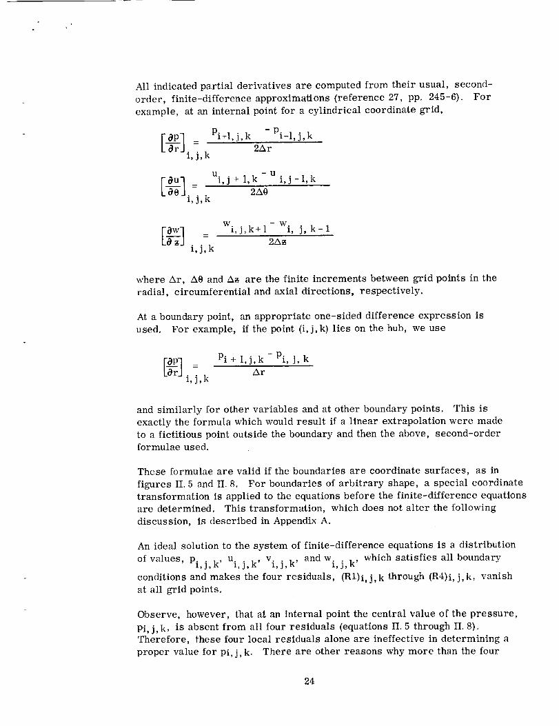
All indicated partial derivatives are computedfrom their usual, second-order, finite-difference approximations (reference 27, pp. 245-6). Forexample, at an internal point for a cylindrical coordinate grid,
Pi+l,j,k - Pi-l,j,k
i, _,k 2Ar
U -U
i, j, k
W. -- W°
1, j,k+l I, j, k-12A_
i,j,k
where Ar, A0 and A_ are the finite increments between grid points in the
radial, circumferential and axial directions, respectively.
At a boundary point, an appropriate one-sided difference expression is
used. For example, if the point (i, j,k) lies on the hub, we use
Pi + 1, j,k - Pi, j, k0[_] --
i,j,k Ar
and similarly for other variables and at other boundary points. This is
exactly the formula which would result if a linear extrapolation were made
to a fictitious point outside the boundary and then the above, second-order
formulae used.
These formulae are valid if the boundaries are coordinate surfaces, as in
figures II. 5 and II. 8. For boundaries of arbitrary shape, a special coordinate
transformation is applied to the equations before the finite-difference equations
are determined. This transformation, which does not alter the following
discussion, is described in Appendix A.
An ideal solution to the system of finite-difference equations is a distribution
of values, Pi,j,k' ui, j,k' vi, j,k' andw.l,j,k, which satisfies all boundary
conditions and makes the four residuals, (R1)i, j, k through (R4)i, j, k, vanish
at all grid points.
Observe, however, that at an internal point the central value of the pressure,
Pi, j, k, is absent from all four residuals (equations II. 5 through II. 8).Therefore, these four local residuals alone are ineffective in determining a
proper value for pi, j, k. There are other reasons why more than the four
24
point resuduals must be considered at a time. These reasons, due to thefinite-difference treatment of boundary conditions, are discussed next.
2. Special Considerations at Boundary Points
At every wall boundary point, the three velocity components must satisfy
the condition of equation (I. 16), which is
W ."_ = 0
In terms of the grid points, this becomes
u. +v. bi, +w. --01, j,k ai, j,k 1, j,k j,k 1, j,kCi, j,k(II. 9)
where ai, j, k, bi, j, k and ci,j, k represent the components of the vector n,normal to the wall boundary at grid point (i,j,k). This immediately im-
poses a dependence of one of the velocity components upon the other two
(see Appendix A), in addition to the relationships already required by the
four governing equations (II. 5) through (II. 8).
One important feature of the present problem is the fact that at each grid
point, there is a system of equations to be satisfied. This poses some
difficulties at boundary points. Note that in a problem involving a single
equation and a single variable, it is sufficient to have the boundary value
of the variable determined solely by the imposed boundary condition without
requiring that the governing finite-difference equation be satisfied there
also (reference 27, pp. 260-265). In our problem, however, four values
(p, u, v, and w) have to be determined at a boundary point. The single
condition (II. 9) is obviously insufficient, especially in view of the fact
that this condition is independent of Pi, j, k. We therefore require that thefour governing finite-difference equations be satisfied at a boundary point
as well as the imposed boundary condition. This is a redundancy of the
entire system of finite-difference equations in terms of the total number of
discrete values. No mathematical inconsistency is implied here, since
the governing equations must be satisfied everywhere in the field, including
the boundaries. However the numerical procedure that we are using
introduces errors because it employs linear extrapolations at the boundaries.
The correct extrapolations are obscure, and we have found the linear ones
to be most practical in this work. Further discussion (see Section II. A. 5)
will demonstrate that the effect of this numerical inconsistency in the boundary
regions vanishes as the finite spacing between adjacent grid points is
diminished.
Over the entire inlet region, the three components of the vorticity vector,
V x _, are specified (see Section I. B). These components are given by
25
- 1E, ,(vxW) r= r Oz (rv(II. 10)
-_- au 8w(v x w) 0 = _ Or
(II. 11)
- :-:E r,rv,-(V x W)z rHI. 12)
It is therefore sufficient to specify the distributions of wi, j, k only on the
first station (k = 1), and ui, j, k and vi, j,k on the first two stations (k = 1, 2)
since, with these specified values, all partial derivatives appearing in the
above three expressions can be computed.
The remaining boundary conditions discussed in Section I. B are imposed
on the finite-difference problem by fixing distributions of Pi, j, k on the
first station and wi, j, k on the last one.
I__t I, J and K denote the total number of radial, circumferential and axial
grid-stations, respectively. Then the total number, E, of governing
finite-difference equations (corresponding to equations (H. 5) through
(n. s)) is
E = 4UK (II. 13)
remembering that p and the F terms are specified by explicit formulae in
terms of pressure and velocity. Since there are then three velocity
components and one pressure to be determined at each grid point, the
total number of discrete variables* is also 4IJK. However, the values of
some of these discrete variables are fixed (as by throughflow boundary
conditions) and some are determined by the values of other variables (as by
wall boundary conditions, equation (II. 9)). Thus the total number, D, of
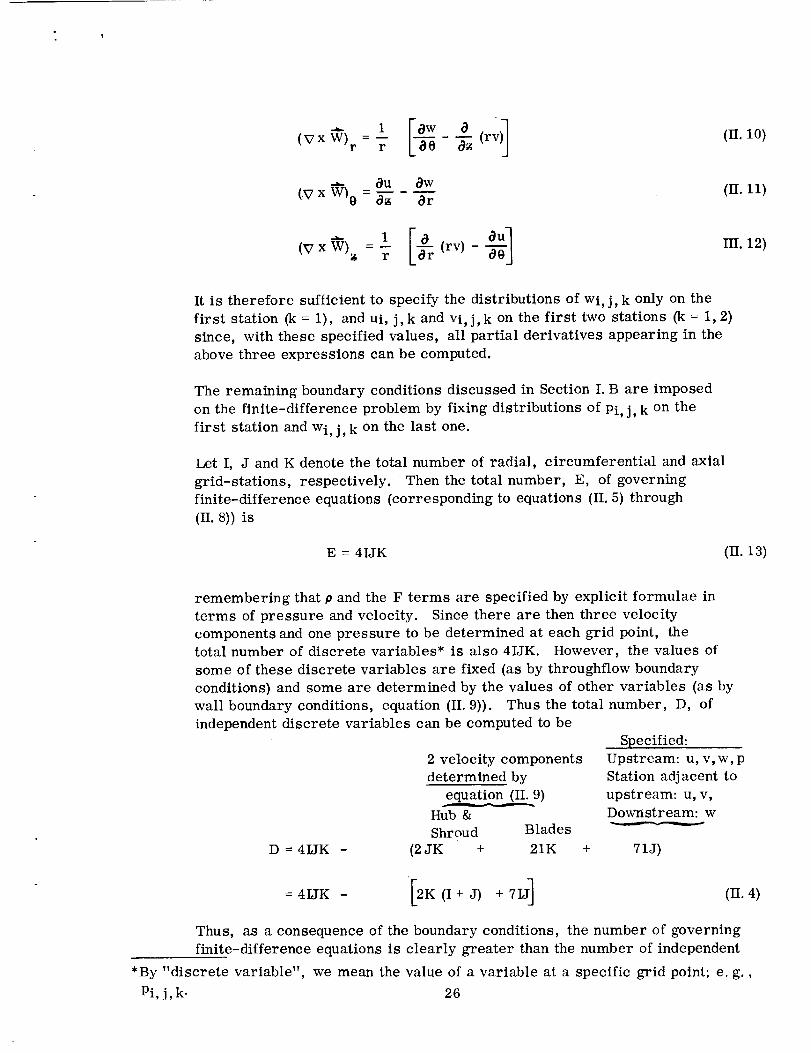
independent discrete variables can be computed to be
2 velocity components
determined by
Hub &Shroud Blades
D=4IJK - (2JK + 21K +
, Specified:
Upstream: u, v, w, p
Station adjacent to
upstream: u, v,
Downstream: w
71J)
=4 K [2K •7.] (..4)Thus, as a consequence of the boundary conditions, the number of governing
finite-difference equations is clearly greater than the number of independent
*By "discrete variable", we mean the value of a variable at a specific grid point; e. g.,
Pi, j,k. 26

discrete variables, (E >D). Such is the nature of the generalboundary value problem, which suggestsa "least-sum-of-squared-residuals" approach, (reference 28, pp. 209-210).
3. Co__o_m_putationalAlgorithm Using Star Residuals
The above observations lead us to define a "total residual"
(II. 15)
i=1 j=l k=l ,j,k (R2)i,j,k (R3)i,j,k j,k
Since the vanishing of all residuals at all grid points is completely
equivalent to the condition R T = 0, the purpose of the computational
algorithm will be to obtain discrete distributions of the three velocity
components and the pressures which will tend to minimize the value of
RT.
A change in the value of a variable at point (i,j, k) can affect the residuals
computed at no more than the seven points of a "star" centered at point
(i, j, k), as shown in figure II. 2. This portion of R T which is affected by a
change at point (i, j, k) will be called the "star residual at point (i, j, k)"
and is defined by
1, j,k i,j,k j,k i,j,k j,k j,
22"where the symbol denotes summation over the seven points of the
i,j,k
star centered at point (i, j, k). (If this central point is a boundary point,
this star may have only 6, 5 or 4 points.) Thus, the method will consist
of determining values of the independent discrete variables at each point
(i, j,k) which will tend to minimize the value of R*i,j, k"
(II. 16)
Considering general applicability and ease of programming, the compu-
tational algorithm which was constructed consists of trying a predetermined
sequence of corrections to each independent discrete variable at each grid
point and accepting only those variations which reduce the value of the local
star residual (and thus reduce the value of the total residual). This procedure
is applied, i'epeatedly cycling through the entire three-dimensional grid of
points until an accuracy criterion (discussed in Section II. A. 4) is satisfied.
27 .:

Specifically, four initial variations are selected: Su, _v, 8w, _p. Also,an integer, M, and a number, 0<a<l, are fixed. At each grid point, thevalue of R'i, ], k is first computed, using the current values of u, v, w, andp at the surrounding grid points. To determine an "improved" value ofui, ],k, for example, R'i, ], k is recomputed, successively using
2 nui, j,k ± _u, ui, j, k • abu, ui,j, k +- a _u ..... ui, j,k± a 6u
until either a reduced value of R'i, j, k is obtained or until n = M, wheren0 < n < M. If one of the variations ui, j, k ± a Su yields a lower value for
R*.l,],k. then that variation is recorded as the new value of ui, j, k.Otherwise, no change is made. Exactly the same procedure is applied
to the other variables and only those variations are accepted which effect
further reductions of R'i, j-', k" The successive treatment, of,,all the ,vgrld"points in the field in this manner constitutes one relaxatmn cycle.
Therefore, by construction, the algorithm guarantees a monotonic
reduction of R T. (We found empirically that M = 3, a -- 0.1 and/iu = 6v = 6w = _p = 0.1 gave good results where the initial distributions
were obtained from one-dimensional calculations, as in Section II. B. 3. )
With each trial variation, the values of Pi, j, k, (Fr)i. j. k, (F0)i, j, k and
(F_)i, j, k are recalculated from the appropriate formulae, before thecorresponding R*.. is recomputed. At a wall boundary point, one of
1, j,kthe three velocity components is selected as dependent upon the other two
(see Appendix A) and its value is computed from equation (II. 9). All
values which are fixed by throughflow boundary conditions are, of course,
not varied.
At the beginning of each succeeding cycle, the magnitudes of Su, 8v, _w
and _p are set equal to the respective maximum values of the variations
which were accepted during the entire previous cycle.
Thus, the magnitudes of the individual trial variations are automatically
decreased as a solution is approached. The values of a and M remain fixed.
It is possible that the theoretical rate of convergence can be improved by a
compound method such as suggested by Marquardt (reference 29) or
Golffeld, Quandt and Trotter (reference 30). We note, however, that both
of these methods ultimately rely on the choice of an "accelerating parameter"
which is successfively varied until the actual numerical value of R T (i. e.
the quadratic functional to be minimized) is decreased. Much additional
empirical work is required to adapt such methods successfully to a given
problem, as evidenced by the following example: We selected a problem
for which we had obtained a solution by the above-described method of successive
variations. We modified the computer program so that the star residual
reduction was accomplished by a gradient technique, based on a second order
28
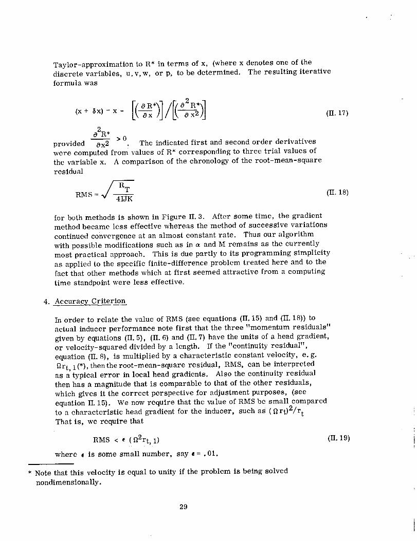
Taylor-approximation to R* in terms of x, (where x denotesone of thediscrete variables, u, v,w, or p, to be determined. The resulting iterativeformula was
(x + $x) --x -
02R *>0
aR* 02R *
provided 0x 2 . The indicated first and second order derivatives
were computed from values of R* corresponding to three trial values of
the variable x. A comparison of the chronology of the root-mean-square
residual
(]I. 17)
(H. 18)
for both methods is shown in Figure II. 3. After some time, the gradient
method became less effective whereas the method of successive variations
continued convergence at an almost constant rate. Thus our algorithm
with possible modifications such as in a and M remains as the currently
most practical approach. This is due partly to its programming simplicity
as applied to the specific finite-difference problem treated here and to thefact that other methods which at first seemed attractive from a computing
time standpoint were less effective.
4. Accuracy Criterion
In order to relate the value of RMS (see equations (II. 15) and (II. 18)) to
actual inducer performance note first that the three "momentum residuals"
given by equations (II. 5), (II. 6) and (II. 7) have the units of a head gradient,
or velocity-squared divided by a length. If the "continuity residual",
equation (1I. 8), is multiplied by a characteristic constant velocity, e.g.
_2rt, 1(*), thenthe root-mean-square residual, RMS, can be interpretedas a typical error in local head gradients. Also the continuity residual
then has a magnitude that is comparable to that of the other residuals,
which gives it the correct perspective for adjustment purposes, (see
equation II. 15). We now require that the value of RMS be small comparedto a characteristic head gradient for the inducer, such as ( _2rt)2/r t
That is, we require that
RMS < , (_22rt, 1)
where _ is some small number, say _ = . 01.
(If.19)
* Note that this velocity is equal to unity if the problem is being solved
nondimensionally.
29

O2
0.3
0.2
0,1
0.0(:;
0.04
0.03
0.02
Method of
Successive
Variations
\ \\
Gradiodnt / O_ _ O
..... C_
0.01 •
0.06
O. 04 i-_[ ]11
0 400 800 1200 1600 2000 2400
Time, Sec.
FIGURE II. 3. COMPARISON OF METHOD OF SUCCESSIVE VARIATIONS AND GRADIENT
METHOD. Root-mean-square, residual (RMS) vs. running time on IBM 7070. (The Univac
1107 that we used in subsequent runs takes about 1,./50 of the time.)
30
If the values of Pi, J, k, ui, j,k, vi, j,k and wi, j, k are randomly distributedabout the "correct" values, then about half of the residuals can be expected
to be positive and the other half negative. The cumulative effect of allresiduals from inlet to outlet for this distribution of variables would result
in a head rise error at outlet which is still much less than _ (_22rt, 1) Am.
Am represents meridional inlet-to-outlet distance along a typical streamline.
However, should a biased distribution of values exist, such as an initial
distribution of p -- o everywhere, then we can expect the residuals to be
dominantly of one sign, (although they might all still be of approximately
the same magnitude as in the above case) and the cumulative effect would
be an error in head rise of order
_(_2 2 rt, 1) Am (II. 20)
From the definition of the static pressure head coefficient for an inducer
Ap/Pf,p =
p ( art, 1)2/go (II. 21)
we see that, in this case, the error in go Ap Pf at the outlet would
/ Am\times the correct head rise of the machine.be comparable to 1
f_I,p
/_ Am\Hence a more realistic convengence requirement would be RMS <_--_ r_t, 1) (_22 rt)but since _ can be chosen to suit specific cases of Am and _I,p,
we have retained generality by stating simply that rt, 1
RMS < e ( f_ 2 rt ' 1). It is therefore advantageous to estimate the initial valuesof the pressure and velocities by a preliminary, one-dimensional calculation
of the flow. This is demonstrated in the discussion in Section II. B. 3.
Finally, if the grid effects or limitations on computing time make it impossible
to achieve negligibly small values of all the residuals, the acceptability of a
particular numerical solution must then be determined by more than just the
value of RMS. In the case of the investigations of our (Section II. B), series
of examples we were limited by computer size and cost to coarse grids.
Thus in most of these examples the numerical procedure (see Section II. A. 2)
made it impossible for us to reduce RMS to the satisfactorily low value
that would make it the only necessary criterion for an accurate solution.
Furthermore this required us to impose a limit on the time or number of
computation cycles, which usually was reached before _ could be achieved.
Therefore, in our presentation of examples in Section II. B we compare the
actual distributions of p, u, v and w with known solutions, whenever possible;and we examine the circulation and other representative quantities in
addition to the behavior of the residuals.
31

5. Effects of Grid Point Density
There :is an effect which the density of grid points has on the minimum
attainable total residual {equivalently, the root-mean-square residual,
RMS, as defined by equation (II. 18)} for a given finite- difference problem
when the method of star residuals is applied. This is due to the linear
extrapolation of the discrete variables which is made at boundary points. :
If it is required that the discrete variables satisfy all governing finite-
difference equations at boundary points in addition to the appropriate
boundary conditions, as discussed in Section II. A. 2, the correct
extrapolation formulae would be required at boundaries in order for
the system of equations to yield zero residual. For example, incorrect
extrapolations which satisfy one differential equation normal to a boundary
will produce boundary values of the variables that will not completely
satisfy the other equations--particularly those that govern motion parallel
to the boundary, Since a linear extrapolation is used, a linear behavior
is forced on the variables in a region extending one grid space from the
boundaries to the interior of the field. For a relatively coarse grid, this
discrepancy will be dominant and, consequently, the total residual, R T,
can only be minimized to some non-zero value. As the grid is refined,
however, the linear approximation to the variables extends over a much
smaller region and the effect of the discrepancy diminishes. Thus theminimum attainable total residual can be expected to approach zero as the
mesh size {distance between adjacent grid points} approaches zero.
To illustrate this effect, we consider the problem of solving, by use of
star residuals, the equations of incompressible flow which is irrotational
in the absolute frame of reference:
W=0
+_2_" =0
We will discuss a two-dimensional solution of these equations over a
region which is a cross section perpendicular to the axis of a paddle-
wheel channel (see figure II. 8). The scalar equations are
(II. 22)
(If. 23)
u Ou 1 Ov--+ _+ -0r _0r r 00
v Oy 1 Ou--+ +21] =0r Or r OO
where u = o on the hub (r = rh) and shroud (r = rt) and v = o on theblade surfaces. * We obtained solutions to this problem, by the method
of star residuals, on grids of 5x 5, 9x7, 9 x 9 and 15x 15 points,
• This special, two-dimensional problem will be referred to again in Section H. B. 2.
(II. 24)
(II. 25)
32
requiring the discrete values of u and v to satisfy the finite-difference
equations resulting from equations (II. 24) and (II. 25) in addition to the
boundary conditions on the hub, shroud and blade surfaces. Each problem
was run to "convergence", i.e. until the root-mean-square residual
(RMS) could not be reduced much further. This yielded essentially the
minimum obtainable RMS. The results (see figure II. 4) indicate that the
minimum attainable total residual approaches zero with diminishing mesh
size. Therefore, any numerical discrepancy (due to requiring that the
discrete variables satisfy all governing finite-difference equations in
addition to the boundary conditions) vanishes as the density of grid pointsis increased.
Another numerical phenomenon, the "take-up effect", is a second order
grid effect that is noticeable especially when coarse grids are employed.
It is the property that yields lower minimum RMS residual results for
a given grid cross-section as the number of independent discrete variables
D (see definition near the end of Section If. A. 2) is increased. The pre-
ceding two dimensional problem is an example. Its minimum RMS residual
is given in Figure II. 4. Extending it axially into the third dimension in-
creases D, adding residuals of the axial component equations which will be
adjusted to non-zero values. (As shown in reference 12, the same two-
dimensional solution is expected on all subsequent r - 0 planes.) This
changes slightly the adjacent downstream two-dimensional distributions,
making it possible to reduce their residuals further than was possible in
the purely two-dimensional problem.
Also, changes to the system of equations or boundary conditions is a way
to change D in a given field. In any case, the residuals thereby added
have the ability to "take-up" some of the error caused by boundary effects,
which process yields a lower minimum RMS, for the given grid cross-
section. Figure II. 9 gives the results for this same problem (using for
initial values the answers that produced the 9 x 7 point in Figure H. 4} as
D was increased over that of the purely two-dimensional 9 x 7 field.
(See Section II. B. 2 for more detail on the problem.) Figure II. 11 shows
that this "take-up effect" is subordinate to the grid-point density one,
because the effect (on minimum RMS) of increasing D is limited R as
might be expected if the two-dimensional 9 x 7 grid cross-section example
we have been using were to be extended infinitely in the axial direction.
Finally, in the normal case of a fixed three-dimensional field with a fixed
system of equations and boundary conditions, D cannot be varied, and there
is no take-up effect -- only the (primary) grid point density effect. However,
as will be demonstrated in Section II. B, we did vary D in some of our
investigations; and these distinctions of grid phenomena must be rememberedas one examines the reBults.
33

O.25
O.20
O.15
0.i0
O.05
0.00
/9x9 Grid
Grid
Grid
(5x5 Grid
0.00 0.01 0.02 0.03 0.04
1/G
FIGURE II. 4 EFFECT OF GRID POINT DENSITY. Minimum attainable root-
mean-square residual (RMS) as a function of the number of grid points (G){ - ._ _ }for two-dimensional solutions of V. W= 0, VxW+ 212 = 0 by star
residuals.
34
6. Form of the Results
The results of a computer run consist of three-dimensional distributions
of relative velocity components, pressures, and the accompanying densities.
These distributions directly indicate blade-to-blade pressure loadings and
inlet-to-outlet velocity distributions on the blade surfaces and their
extensions. But to obtain the customary overall performance parameters,
certain averaged quantities must be extracted from these distributions.
For this purpose a data reduction program was written. Details of this
program are presented in Appendix C.
The mass-averaged parameters are calculated from finite-difference
approximations of the following formulae:
Static Pressure Head
Srh rdrd0Pp) = WT (1]. 26}
where the total mass flow rate across the inlet plane of one channel is
calculated from
rt ,.0sw w f J^ ( p w) rdrd0-- z
nb r h _ p(II. 27)
Absolute Velocity Head
f rt f:; _2"_ol Iu 2 + (v+ r12)2+w2] (pw)
(2V-_) = rhw T
r drd0
(II.28)
Input Energy
(uvo) --
r tfrh fg0; Erl_ (v+r_)] (pw) rdrd0
WT
The above three quantities are calculated at the channel inlet and at the
outlet. From these we obtain ......
(H. 29)
35

Total Head Rise
1 1
(1"[.30)
Shaft Power Delivered to Fluid
n--_- go (II. 31)% 2
Overall Efficiency
77 _ AH w T (II 32)P
S
Further details of the calculations are given in Appendix C.
B. APPLICATION AND RESULTS
The results of applying the method of solution to a sequence of problems are presented
in this section. The problems were solved in order of gradually increasing complexity,
and Table II. 1 shows the purpose and general result of each one. We employed three
types of geometry to determine a) the ability of the program to proceed to a correct
solution, b) the grid effects and attainable accuracy and c) the applicability to inducer
flow analysis.
The specific geometries were
(1) Paddle-wheel channel with wheel-type axial flow (liquid and two-phase).
(2) Paddle-wheel channel with irrotational, incompressible, axially constant
flow (reference 12).
(3) Two typical, variable-lead inducer channels, including upstream and
downstream flow regions (liquid and two-phase).
The geometry of each channel is presented, followed by selected numerical results
and a discussion of some of the phenomena which they illustrate. All problems are
solved nondimensionally, according to the system presented at the end of the List of
Symbols prior to Section I.
36

<
Z
©
¢/]
©
0
_-
o__O
O
Z2;<
rO
o
O
O
O0
¢._
O
_._
_S
d
OO
d
"r
I
0
O O
N__._
o _.1,.o ,_ o
¢0 "" _"_ O
8 .a_
O
O _
O O
_u
I
d
ca.I
O
I
"l:J
O O
r_ I
O _ _
, .,,o O
O _
.0
O %
_2
O
O '_ -
_ _ i
_o gl
m_
I
,6I
e_m
,o_
0
0 0
_b
O
d_
_._ _i_o0a,
_ .,.._ ,
_, 0
o3_o N "_
_ O
O%_u
_._
O %
O
d_
_ m m
_._1
o"
_ e
0
_._
I .......
I
e-
_o0 .s_ °_"
I
37
O
_°. ag
_ _ h._
_ _
+a _ ,._ _ 0
_ 2? s
m
_g
I I
M _
N_O
IO
I1)
I0
dN
N
t
__ _"T
_ h
o_
_ _
_8
0
0
o_
&
_,_

1. Paddle-Wheel Channel With Wheel-Type Flow
The geometry of this six-bladed channel is shown in figure H. 5. The
primary purpose of solving the first two problems on a 3 x 3 x 3 grid
was to have a simple checkout of the computer program. Due to the
special shape of the channel, the wall boundary conditions {equation
{II. 9)) are simply
Uh= ut =0"0 }Vs= Vp= 0.0
Boundary conditions, known correct answers, and obtained results are
shown in tables II. 2 and II. 3. Initial assumptions for both runs were
made to differ from their correct values randomly by about 0.2.
Run E-l: All Liquid Flow
The correct solution has
u=0.0}
v 0.0 everywhere
w 1.0
The only pressure gradient is in the radial direction. Integration of this
radial gradient gives
1 _22
P=Ph + _ Of _oo (r2. rh2)
Setting Ph -- 0, this gives correct answers of the continuous problem as
ph = 0.0
PM = 0. 16406
Pt = 0.46875
where the subscript M denotes the grid point half-way between hub and
tip. Solving the finite-difference analogs of equation (H. 5) simultaneously
at the three grid points, however, gives
(II. 33)
H. 34)
38

\
r h
,Axis of Rotation
FIGURE II. 5. PADDLE-WHEEL CHANNEL FOR WHEEL-TYPE, AXIAL
FLOW CALCULATIONS. Runs E-l, 2.
\
39
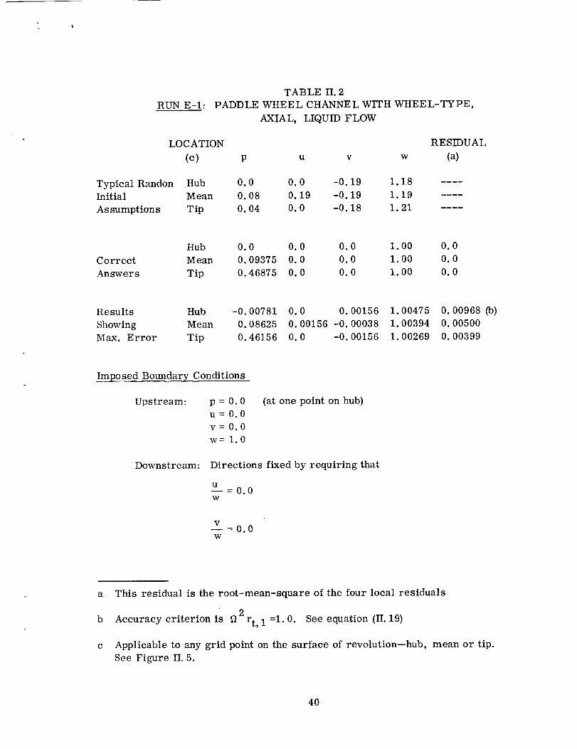
RUN E-l:
TABLE II. 2
PADDLE WHEEL CHANNEL WITH WHEEL-TYPE,
AXIA L, LIQUID F LOW
LOCATION
(c)
RESIDUAL
p u v w (a)
Typical Randon HubInitial Mean
Assumptions Tip
0.0 0.0 -0.19 1.18
0.08 0.19 -0.19 1.19
0.04 0.0 -0.18 1.21
mmWw
Hub
Correct Mean
Answers Tip
0.0 0.0 0.0 1.00 0.0
0.09375 0.0 0.0 1.00 0.0
0.46875 0.0 0.0 1.00 0.0
Results Hub
Showing Mean
Max. Error Tip
-0.00781 0.0 0.00156 1.00475
0.08625 0.00156 -0.00038 1.00394
0.46156 0.0 -0.00156 1.00269
0.00968 _)
0.00500
0.00399
Im_po sed _ Conditions
Upstream: p=0.0u=0.0
v=0.0
w=l.0
(at one point on hub)
Downstream: Directions fixed by requiring that
Um=0.0w
V-0.0
w
a This residual is the root-mean-square of the four local residuals
b Accuracy criterion is _2 rt, 1 =1.0. See equation (II. 19)
c Applicable to any grid point on the surface of revolution--hub, mean or tip.
See Figure II. 5.
4O
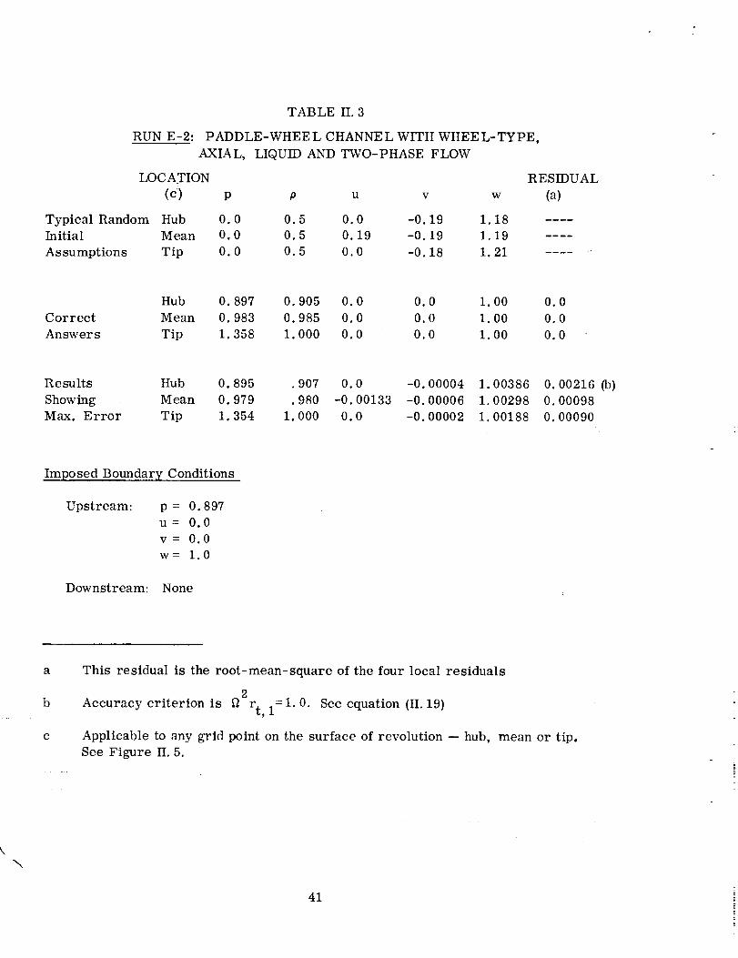
RUN E-2:
TABLE II. 3
PADDLE-WHEE L CHANNE L WITH WHEE L-TYPE,
AXIAL, LIQUID AND TWO-PHASE FLOW
p U V w
0.5 0.0 -0.19 1.18
0.5 0.19 -0.19 1.19
0.5 0.0 -0.18 1.21
LOCATION
(c) p
Typical Random Hub O. 0Initial Mean O. 0
Assumptions Tip O. 0
RESIDUAL
(a)
Hub 0. 897
Correct Mean 0. 983
Answers Tip 1. 358
O.905 O.0 O.0 1.O0 O.0
O. 985 O.0 O.0 1.O0 O.0
I.000 O.0 O.0 1.O0 O.0
Results Hub 0. 895
Showing : Mean 0. 979
Max. Error Tip 1. 354
.907 0.0 -0.00004 1.00386
.980 -0.00133 -0.00006 1.00298
1o000 0.0 -0.00002 1.00188
0.00216 _)
0.00098
0.00090
Imposed BoundaryConditions
Upstream: p= O.897
u-- 0.0
v= 0.0
w-- 1.0
Downstream: None
a
b
C
This residual is the root-mean-square of the four local residuals
Accuracy criterion is l_2
--1.0.rt, 1 See equation (H. 19)
Applicable to any grid point on the surface of revolution -- hub, mean or tip,
See Figure H. 5.
\
41

Po = 0.0
PM = 0. 09375
Pt = 0.46875
The discrepancy at point M is due to the linear approximations made at
the hub and tip points.
In Section II. A. 5 we explained that incorrect extrapolations would not
satisfy all the differential equations simultaneously. However in this
example we have simply a one-dimensional problem because the answers
yield no variation in the axial and tangential directions with only one
equation (H. 34). Thus it is possible to attain all zero residuals, although
the results for the discrete problem disagree at one point with the solution
of the continuous problem. (See the discussion of 'Vdiscretization error v'
in reference 27). Results of this problem are shown in figure II. 6 and
table H. 2.
Run E-2: Liquid and Two-Phase Flow
For this problem, we were able to determine values of Ph, PM' and
Pt so that, for Pf = 1.0, Psat = 1.0 and T* = 1.0 (see equations (I. 7)
and (I. 8), it was again possible to have all residuals equal to zero
in the finite-difference solution. Using the same initial assumptions
for velocities as in Run E-1 and zero for pressures, figure II. 7 shows
that after 110 relaxation cycles the RMS value continues to approach
zero, as expected for this case. Table II. 3 shows how close the results
are to the known, correct values. We observed that inclusion of the
state equation in the computations did not cause any perceivable increase
in running time per relaxation cycle.
2. Paddle-Wheel Channel with Irrotational Flow
The geometry for this channel is shown in figure H. 8. The hub-to-tip
radius ratio as well as the blade-to-blade angles were obtained directly
from figure 2 of reference 12. The channel which we consider here is a
portion of the channel used by Ellis and Stanitz (for which complete,
detailed results are presented in reference 12) upstream of where the
effects of radial flow are felt. This is a hypothetical problem since
the paddle-wheel portion of the channel would have to extend infinitely
far upstream in order to yield an irrotational, axially constant flow
pattern.
However, it is another problem whose numerical solution can be determined
by simpler methods. This problem also demonstrates the finite-difference
42

0.6
0.4
0.3
0.2
0.1
0.06
_0.04
0.03
0.02
0.01
O.006
O.004
O.003
o\
2 4 6 8 10 12 14 16
Cycles
FIGURE II. 6. INCOMPRESSIBLE, LOSSLESS, WHEEL-TYPE FLOW. Run E-1.
Root-mean-square residual (RMS) vs. number of relaxation cycles.
43

0.6
0.4
0.3
0.2
0.1
0.06
0.04
0.03
ot]
0.02
0.01
O. 006
0. 004
0.003
0.002
0.00120 40 60
Cycles
80
FIGURE H. 7. TWO-PHASE, LOSSLESS, WHEEL-TYPE FLOW.
square residual vs. number of relaxation cycles.
44
100 120
Run E-2. Root-mean-
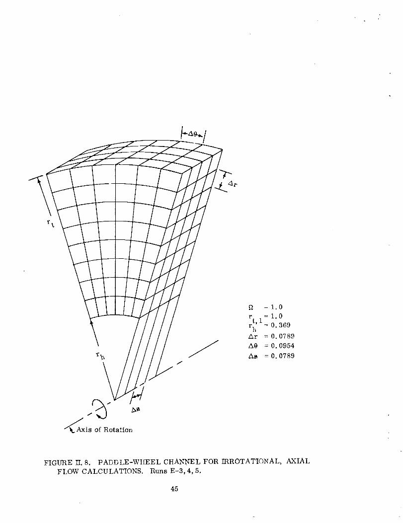
_2 =1.0
r t = 1.0r ' 1 = 0. 369
hAr = 0. 0789
A0 = 0. 0954
A_ = 0. 0789
_is of Rotation
FIGURE II. 8. PADDLE-WHEEL CHANNEL FOR IRROTATIONAL, AXIAL
FLOW CALCULATIONS. Runs E-3,4, 5.
45

phenomenonof our methodwhich is called the "take-up effect".
The solution of this special three-dimensional problem is merely anaxial propagation of a two-dimensional flow pattern with relativerotation of 2 _2. It is, therefore, a propagation in the _ -direction ofthe solution of the equations
u + Ou + 1 Ov -0r Or r O0
v Ov 1 Ou_+ +2ft =0r Or r O0
(II. 24)
(II. 25)
This problem was presented in Section II. A. 5. As starting values forvelocities in the three-dimensional problem, we used the numerical
results of the two-dimensional problem on a 9 x 7 grid and applied them
at all axial stations, along with a constant through-flow velocity of
w = 1, 0. Initial distributions for pressure were obtained from
,u22, v2,2,1P=Po +- (r-ro2)- -u2g o o(H. 35)
which is a consequence of applying the streamline component of the
momentum equation (I. 4) with an assumption of constant "inlet"
pressure infinitely far upstream. The subscript o denotes a reference
point, arbitrarily selected at the intersection of the "pressure blade"surface with the hub. The corresponding initial RMS value is 0. 169.
This RMS value is not zero because of the effect of the relatively coarse
grid, explained in Section II. A. 5, (see the 9 x 7 point in Figure II. 4).
On the upstream throughflow boundary of this channel, we fixed the
distributions of u and v in accordance with the results of the two-
dimensional irrotational flow problem solved in Section H. A. 5.
The w distribution on that boundary was set at unity and we fixed the
value of Po at the reference point of equation (II. 35). On the downstream
throughflow boundary, we imposed flow directions by fixing the values
of the ratios u/w and v/w, usingtheupstreamdata. Although this set of
boundary conditions is valid since they are known results, the impossibility
of determining downstream flow directions for the general inducer problem
is apparent. For a discussion of alternate throughflow boundary conditions,
please see Section I. B. 2.
For this problem, the following three runs were made:
46

Run E-3:9 x 7 x 3 Grid With Exit Flow Directions Fixed
Since this is solved three-dimensionally, we will not require the axial
derivatives to be zero. Therefore, all values on the second and third
axial planes are free to readjust so as to improve the radial and
circumferential residual nonequilibrium at the sacrifice of small axial
gradients in accordance with the "take-up effect, " and the resulting
RMS value after ten relaxation cycles is 0. 090 (see figure H. 9).
The amount of readjustment which occurs due to the take-up effect
is small as can be seen in figure II. 10.
Run E-4: 9 x 7 x 3 Grid With Exit Flow Directions Free
With the same grid of points as for the previous run, we lifted the
downstream requirement that the ratios u/w and v/w have specified
values. (See discussion below.) This introduced more independent
discrete variables D for the same number of governing finite-difference
equations (see Sections II. A. i and 2). As in the previous run, this
permitted more readjustment of the variables to further reduce the
residual amount of nonequilibrium and the results of 20 cycles for this
run are shown in figures II. 9 and II. 10.
Run E-5" 9 x 7 x 5 Grid With Exit Flow Directions Free
Again using the same grid spacing as in the previous two runs, but
extending the channel by adding two axial stations, we made another
2-cycle run. The additional axial stations enabled further "take-up"
of axial gradients and a further reduction of the minimum RMS value
was attained (figure II. 9).
The lifting of the downstream throughflow direction requirement did
not result in a radically different flow pattern (see figure II. 10) probably
because the initial distributions were very close to the correct values.
A complete set of boundary conditions is still required for the general
problem (see Section H. B. 3).
In all three of these runs the coarse grid-point density caused the minimum
RMS residual to be too high to serve as the only criterion for judging the
accuracy of the solutions. In fact (as will be seen) it is quite possible for
the answers to be correct on the average but for the minimum RMS to be
high, as was discussed in Section II. A. 4. Further, in the absence of
any "take-up" by axial gradients-- as is the case in our two dimensional
solution of equations (II. 24) and (II. 25) (see Figure II. 4) -- the effects
of the relatively large resulting RMS residual appear to be felt mainly
in a fairly uniform way near boundaries, tending to yield better average
answers. The take-up effect, while reducing the minimum obtainable
47

0.2
OC
0.1
0.08
0.06
0.04
I t I t I I t n IO Run E-3:9x7x3 Grid with Downstream Flow Directions Fixed
p Q Run E-4:9x7x3 Grid with Downstream Flow Directions Free
/X Run E-5:9x7x5 Grid with Downstream Flow Directions Free
I .... ----7 ............
I
C
._"c
n
Cycles
24
FIGURE II, 9. FEMONSTRATION OF TtIE "TAKE-UP EFFECT" WITH INCOMPRESSIBLE,
IRROTATIONAL FLOW. Root-mean-square residual 0tMS) vs. number of relaxation
cycles.
48

¢9O
(D
¢D
¢9
L)¢9
¢0
0.24 _ :
o, 20 _
0.16 ___
0.12
0.08
O. 04
0.00
-0.04
-0.08
-0.12
['1 Results of Run E-3
\
A Results of Run E-4
\O Results of Run E-5-0.16
-0.20
-0.24
-0.28
-0.32
rh Radius, r (See Figure H. 8) rt
(Hub) (Tip)
FIGURE II. 10. VELOCITIES IN INCOMPRESSIBLE, IRROTATIONAL FLOW.
Distributions along channel center line on exit plane.
49

I
RMS residual, never reduces it far enough to guarantee accurate answers--
and it propagates errors (especially axially). The net result of the take-
up effect -- as long as coarse grids are used -- is then a decrease in the
accuracy of the average answers. Examination of the relative circulation
around the perimeter of the passage at exit -- a useful criterion of average
accuracy -- will demonstrate this point.
Figure II. 10 shows that the largest deviations in the velocity fieldoccur close to the hub. With this we expect to see a corresponding
change in the calculated circulation, F.
By definition
where the integral is taken around the boundary of a channel cross
section.
By Stokes' Theorem
f_ _F= V xW .dA
where the integral is taken over the entire area of the cross section.
Since
VxW =-2_
for irrotationality (see reference 9, p. 11), we have
F--- fA 2_ . d-_=- f_(rt2- rh2 ) (0 s- 0p)
Calculating the absolute value of this with the dimensions shown in
Figure II. 8, we obtain the theoretical circulation for this problem as
Ftrue = 0. 49444. Substituting boundary velocities into an approximation
to equation (II. 36) and comparing these calculated values of circulation
at exit to the theoretical value we have the following table of results:
(g. 36)
(ll. 37)
(II. 38)
(II. 39)
5O
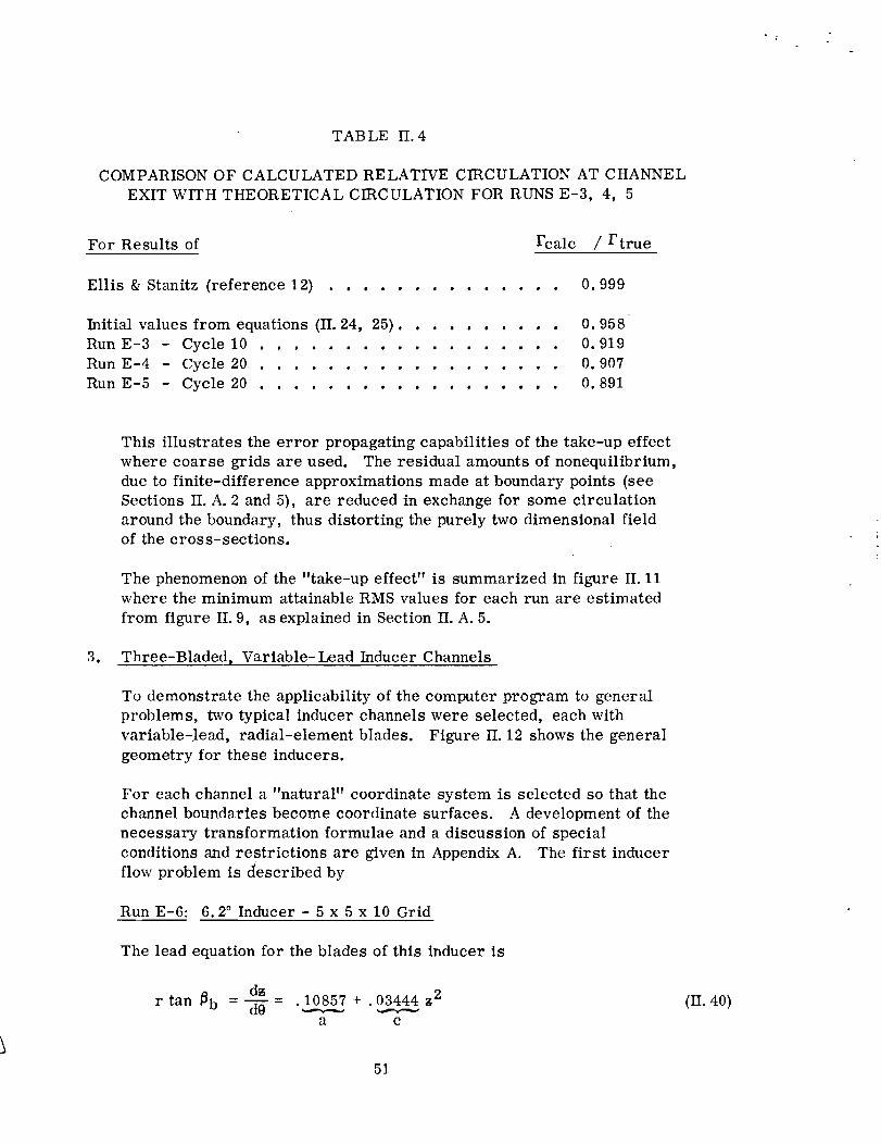
TABLE II. 4
COMPARISONOF CALCULATED RELATIVE CIRCULATION AT CHANNELEXIT W_H THEORETICAL CIRCULATION FORRUNSE-3, 4, 5
For Results of Fcalc / Ftrue
Ellis & Stanitz (reference 12) .............. 0. 999
Initial values from equations (II. 24, 25) .......... 0. 958
Run E-3 - Cycle 10 .................. 0.919
Run E-4 - Cycle 20 .................. 0.907
Run E-5 - Cycle 20 .................. 0. 891
This illustrates the error propagating capabilities of the take-up effect
where coarse grids are used. The residual amounts of nonequilibrium,
due to finite-difference approximations made at boundary points (see
Sections II. A. 2 and 5), are reduced in exchange for some circulation
around the boundary, thus distorting the purely two dimensional field
of the cross-sections.
The phenomenon of the "take-up effect" is summarized in figure II. 11where the minimum attainable RMS values for each run are estimated
from figure II. 9, as explained in Section H. A. 5.
3. Three-Bladed, Variable-Lead Inducer Channels
To demonstrate the applicability of the computer program to general
problems, two typical inducer channels were selected, each with
variable-lead, radial-element blades. Figure H. 12 shows the general
geometry for these inducers.
For each channel a "natural" coordinate system is selected so that the
channel boundaries become coordinate surfaces. A development of the
necessary transformation formulae and a discussion of special
conditions and restrictions are given in Appendix A. The first inducer
flow problem is described by
RunE-6:6.2 ° Inducer- 5x 5x10 Grid
The lead equation for the blades of this inducer is
d_ 10857 + 03444 _2r tan _b = d--'_= '----_ ",-_---_
a c
51
(H. 40)
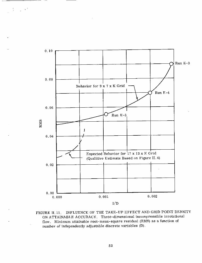
Tl
_o
0.10
0.08
0.06
0.04
0.02
/f
/J/L__
x 7 x K Grid
a¢
Behavior for 9
I
//
Expected Behavior for 17 x 13 x K Grid
(Qualitive Estimate Based on Figure II. 4)
)00 0.001 0.002
I/D
Run E-3
FIGURE II. 11. INFLUENCE OF THE TAKE-UP EFFECT AND GRID POINT DENSITY
ON ATTAINABLE ACCURACY. Three-dimensional incompressible irrotational
flow. Minimum attainable root-mean-square residual (RMS) as a function of
number of independently adjustable discrete variables (D).
52

a) View Into Inlet '
Notes on Geometry_ L
Three radial-element blades.
Lead equation for pressure side of blade:
dO 20.10857 -- 0.03444
d_
Solidity: ¢ = 5.9
Suction sides of blades faired from zero
at _, = 0.0 to full thickness at _ - 0. 1086.
Full thickness maintained thereafter,
Linear dimensions given in units of tip radius.
0.0238
Suction Blade
Side Thickness
Side
Deyeloped View of
Blade Tip
Upstream Extension of Blade
j3 flow 4.8 °
t/b = 6.2 °
o
FIGURE II. 12. VARIABLE-LEAD INDUCER GEOMETRY FOR 6.2 ° BLADE TIP INLET ANGLE.
53

r¢
where _ -- 0 at the blade leading edge. This gives blade tip angles of 6.2 °
and 11.5 °, respectively, at the leading and trailing edges.
The finite-difference grid includes one station at a distance of approximately
one-half of a channel width upstream of the blade leading edge. The angle
of these upstream stagnation surfaces is chosen so that
dOds w " (H. 41)
For a nondimensional rotative speed of _2 = 1.0 and inlet axial velocity
of w I = 0. 08302, this results in an inlet incidence angle of i = 1.45 °.
The initial throughflow velocities, w, are made to vary linearly from
inlet to outlet where the trailing edge distribution is the one which resulted
from an earlier version of Run A-1 (see Section III. B. 1). These velocities
turned out to be approximately 7% low at exit due to failure to allow for
blade blockage (see figure III. 5). Therefore, this is equivalent to a
physical incompatibility in that "less comes out than goes in". The
method of star residuals, however, still finds a solution with minimum
total residual for the imposed boundary conditions. The remaining runs
in this section demonstrate that this inconsistency in the specified exit
velocity does not affect the basic nature of the resulting velocity
distributions.
The radial velocities, u, are distributed linearly from hub to shroud at
each axial station, so that they are estimated by
drU=W -
d_
dr
where the slope _ varies linearly from hub to shroud. The relative cir-cumferential velocities are estimated by
dOv=wr m
d_
dOwhere .----- is an average, measured halfway between the blade surfaces ateach axial station. This is done in order to get a fair approximation of
the unknowns at the beginning of the problem. For the same reason, initial
pressures are calculated at each grid point from
-2goPf (r 2 _22+wl 2-u 2-v 2-w 2) (II. 42)P
which is a consequence of integrating the momentum equation (I. 12) along
streamlines with the above velocity components and p = 0 on the upstream
axial plane.54
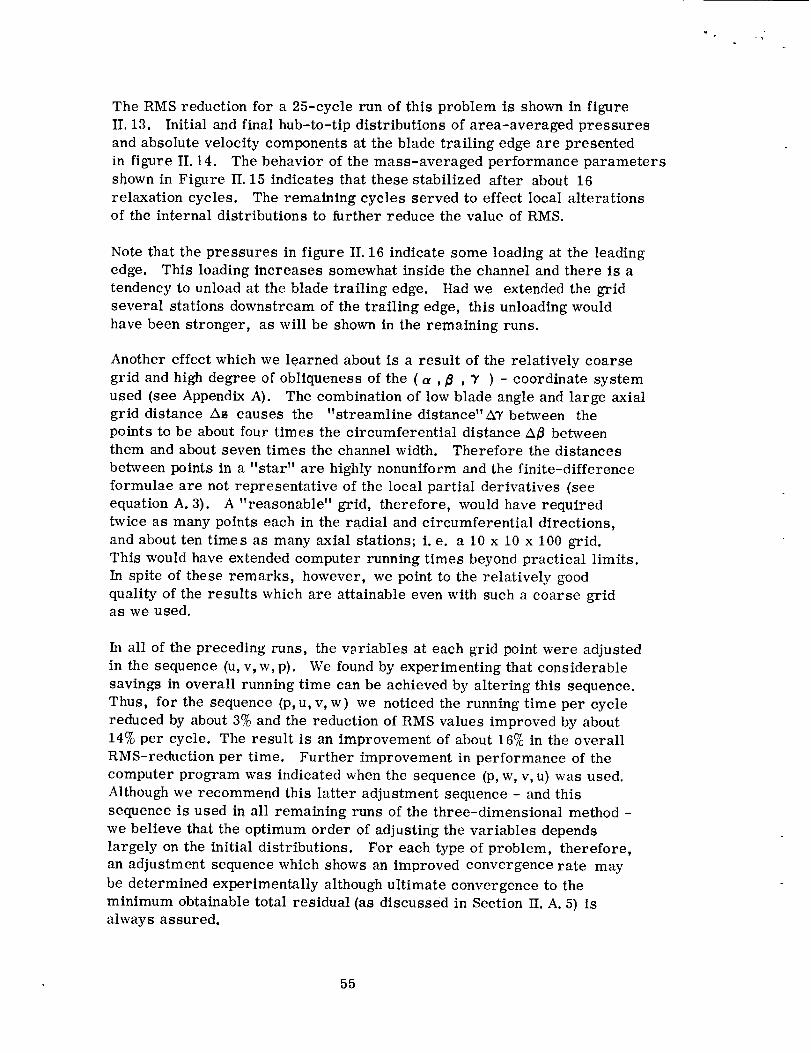
r
The RMS reduction for a 25-cycle run of this problem is shown in figure
II. 13. Initial and final hub-to-tip distributions of area-averaged pressures
and absolute velocity components at the blade trailing edge are presented
in figure II. 14. The behavior of the mass-averaged performance parameters
shown in Figure II. 15 indicates that these stabilized after about 16
relaxation cycles. The remaining cycles served to effect local alterationsof the internal distributions to further reduce the value of RMS.
Note that the pressures in figure II. 16 indicate some loading at the leading
edge. This loading increases somewhat inside the channel and there is a
tendency to unload at the blade trailing edge. Had we extended the grid
several stations downstream of the trailing edge, this unloading would
have been stronger, as will be shown in the remaining runs.
Another effect which we learned about is a result of the relatively coarse
grid and high degree of obliqueness of the ( a , _ , _' ) - coordinate system
used (see Appendix A). The combination of low blade angle and large axial
grid distance A_ causes the "streamline distance"A_ between the
points to be about four times the circumferential distance/x_ between
them and about seven times the channel width. Therefore the distances
between points in a "star" are highly nonuniform and the finite-difference
formulae are not representative of the local partial derivatives (see
equation A. 3). A "reasonable" grid, therefore, would have required
twice as many points each in the radial and circumferential directions,
and about ten times as many axial stations; i.e. a 10 x 10 x 100 grid.
This would have extended computer running times beyond practical limits.
In spite of these remarks, however, we point to the relatively good
quality of the results which are attainable even with such a coarse gridas we used.
In all of the preceding runs, the v_riables at each grid point were adjusted
in the sequence (u, v,w, p). We found by experimenting that considerable
savings in overall running time can be achieved by altering this sequence.
Thus, for the sequence (p,u, v,w) we noticed the running time per cycle
reduced by about 3% and the reduction of RMS values improved by about
14% per cycle. The result is an improvement of about 16% in the overall
RMS-reduction per time. Further improvement in performance of the
computer program was indicated when the sequence (p, w, v, u) was used.
Although we recommend this latter adjustment sequence - and this
sequence is used in all remaining runs of the three-dimensional method -
we believe that the optimum order of adjusting the variables depends
largely on the initial distributions. For each type of problem, therefore,
an adjustment sequence which shows an improved convergence rate may
be determined experimentally although ultimate convergence to the
minimum obtainable total residual (as discussed in Section 1I. A. 5) isalways assured.
55

t
0.1O. 09
0.08
0.07
0.06
0.05
O. 04
0.03
0.02
\\\
0.012 4 6 8 10 12 14 16 18 20 22 24
Cycles
FIGURE II. 13. RESIDUAL RELAXATION DATA FOR INCOMPRESSIBLE,
LOSSLESS FLOW IN 6.2 ° INDUCER. Run E-6. Root-mean-square
residual vs. number of relaxation cycles.
56
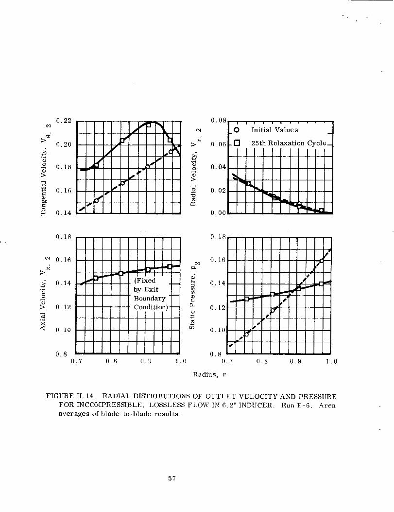
0.22
> 0.20
,rll
o 0.18O
0.16
O. 14
/
gv
f
I/ k
f,J
0.08
g,q
> 0.06
°r'l
o O. 04
>
0.02
0.00
I
_O
.fl
II!
i | ! | t • i • ,
Initial Values !25th Relaxation Cycle_
ll|llll
0.18
0.16 ' --
I> _ ,,,_ ;,,d ],,, _,_ _ -_"C"
0.14-4 _---_-- : (Fixed .--._ by ExitO
O
>
<
0.12
0.10
Boundary
Condition)---
¢-q
d
¢9
0.18
pO_ •
0.16
0.14
0.12
0,10
0.80.7
Radius, r
_ m
xv
S
°8 -- _
0.7 0.8 0.9 1.0 0.8 0.9 1.0
FIGURE II. 14. RADIAL DISTRIBUTIONS OF OUTLET VELOCITY AND PRESSURE
FOR INCOMPRESSIBLE, LOSSLESS FLOW IN 6.2 ° INDUCER. Run E-6. Area
averages of blade-to-blade results.
57
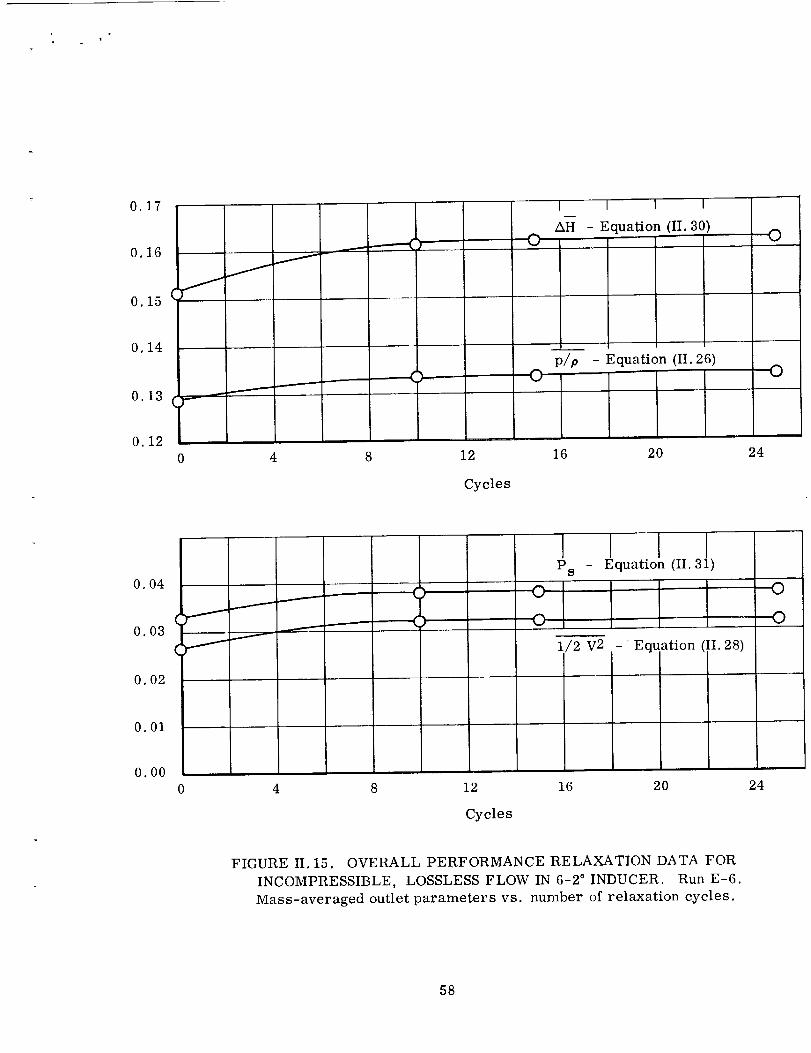
J
0.17
0.1.6
0.15
0.14
0.13
0.12
J
W--
Jv
f_
0 4 8
()
12
Cycles
O
I i ] I
AH - Equation (II. 30)
p/p - Equation (II. 26)O
16 2O 24
O
O
0.04
(0.03
(
0.02
0.01
0.00
0
O
O
Ps - Equation (II.31)
1/2 V2 -Equ.ation (.II. 28)
4 8 12 16 20
Cycles
O
O
24
FIGURE II. 15. OVERALL PERFORMANCE RELAXATION DATA FOR
INCOMPRESSIBLE, LOSSLESS FLOW IN 6-2 ° INDUCER. Run E-6.
Mass-averaged outlet parameters vs. number of relaxation cycles.
58

b
o
or,4
16
14
12
10
O8
O6
O4
O2
Pressure
Surface
O
Suction
Surface
d
O- O
O
%#
A
rfv
.14 L.__l_....
IV
1 4
u
I0
O8
o O1
7 i0
Axial Distance
O6
O4
02
I
Y
T"r
13 16
FIGURE II. 16. AXIAL DISTRIBUTIONS OF BLADE SURFACE PRESSURE
FOR INCOMPRESSIBLE, LOSSLESS FLOW IN 6.2 ° INDUCER: Run E-6.
59

,-_
o
.l.0
.9
.8
.7
Pressure
Surface
0
Suction
Surface
d
0_
o 9
.6
.5
I_I .4
.3
0.2
a
D-
0
FIGURE II. 17.
1 4 7 I0 13 16
Station
AXIAL DISTRIBUTION OF BLADE SURFACE VELOCITY
FOR INCOMPRESSIBLE LOSSLESS FLOW IN 6.2 ° INDUCER: Run E-6.
6O
In view of the above observations, we next analyzed an inducer channel
of the same overall dimensions as the above one but with higher blade
angles. The grid we selected has 2.2 times as many points, and we
extended the flow field upstream and downstream of the blades by an
axial distance equivalent to approximately one channel width. This
is consistent with other numerical calculations of fluid flow fields (see,
for example, references 23 and 24). The geometry used for the remain-
ing computer runs is shown in figure II. 18.
The lead equation for the pressure surfaces of the blades of this inducer is
d_ _ 2
r tan B b - dO _' 21256 + ._09830 _a c
(II. 43)
where _ = 0 at the blade leading edge. This gives blade tip angles of
12 ° and 24.5 °, respectively, at the leading edge (_ = 0.0) and the trailing
edge (z = 1. 62857).
The finite-difference grid includes three axial stations each upstream
and downstream of the blade system. The angle for the upstream stag-
nation surfaces is again calculated from equation (II. 41). With an inlet
axial velocity of w = 0. 17633, this results in an incidence angle of 2 ° atthe leading edge, which was chosen as a representative value for theseinducer calculations.
The initial throughflow velocities, w, are chosen so that mass con-
servation is satisfied one-dimensionally from inlet to outlet. As was
done in the case of the 6.2 ° inducer, the radial velocities, u, are
distributed linearly from hub to shroud at each axial station so that
h
where(dd-_h is the slope of the hub. The relative circumferential
velocities are given by
dOv=wr_
d_dO
where dz is an average, measured halfway between the blade surfacesat each axial station.
61
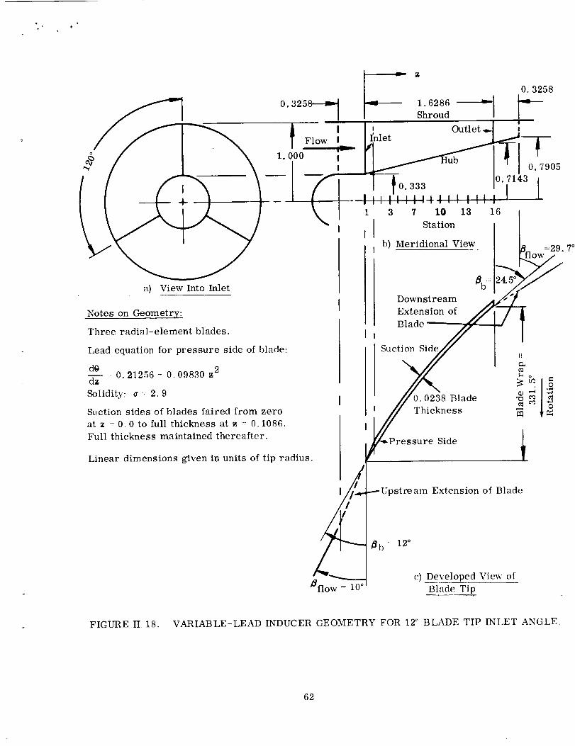
0. 3258---_ 1. 6286
! Shroud
Flow I let Outlet ._
.ooo ;=
]4_-4411! III I3 7 10 13 16
] Station
J ' b)Meridional View
a) View Into Inlet _b::
Downstream
Notes on Geometry_i Extension ofBlade
Three radial-element blades.
Lead equation for pressure side of blade:
dO 0. 21256 + 0. 09830 z 2d_
Solidity: _- 2.9
Suction sides of blades faired from zero
at z : 0.0 to full thickness at _ - 0. 1086.
Full thickness maintained thereafter.
Linear dimensions given in units of tip radius.
_flow--- 10 °
Suction Side
• 0238 Blade
Thickness
Side
.---Upstream Extension of Blade
b 12 °
c) Developed View of
Blade Tip
0.3258
!
0. 7143! l
=29.7 °
FIGURE II. 18. VARIABLE-LEAD INDUCER GEOMETRY FOR 12 _ BLADE TIP INLET ANGLE.
62
Initial values of pressures are again calculated from
Pf (r 2 _2 + Wl 2 2 2 2=_ -U -V -W )P 2g o
(II. 42)
The downstream stagnation stream surfaces are initially selected so that
no energy is added to the flow downstream of the blade trailing edge. We
simulate this condition by requiring that V0 remain axially constant for
constant r. Since
V= V 0 - rl2
this is equivalent to requiring that
v
r remain constant. But
dO 1 v vA
d_ tan Bb w q(1I. 44)
where A is the channel cross section area and q is the constant volume
flow rate. Therefore the stagnation stream surface angles are calculatedfrom
d0 - (r--_qA (lI. 45)
i.e. the rate of change of angle with axial distance is proportional to
cross section area. Note that finally the only way to obtain no energy
addition by the stagnation stream surfaces is to adjust them and re-
compute until no pressure difference exists across them.
RunE-7:12 ° Inducer- 5 x 5x 22 Grid
The first run with the above described inducer channel was made for
an incompressible, lossless fluid. Figure II. 19 shows that the value
of RMS is still being reduced after fifteen relaxation cycles. As was
the case for Run E-6, however, we see that the values of relative
circulation (figure II.20) have reached their final levels by the eighth
relaxation cycle. In figure II. 22 we present a chronology of the hub-
to-tip distributions of the pressures and velocity components at the
inducer exit plane. The final pattern for these area-averaged quantities
has emerged by the 15th relaxation cycle.
The resulting hub-to-tip distribution of absolute circumferential velocity
V 0 is not one which would be expected from simple radial equilibrium
63
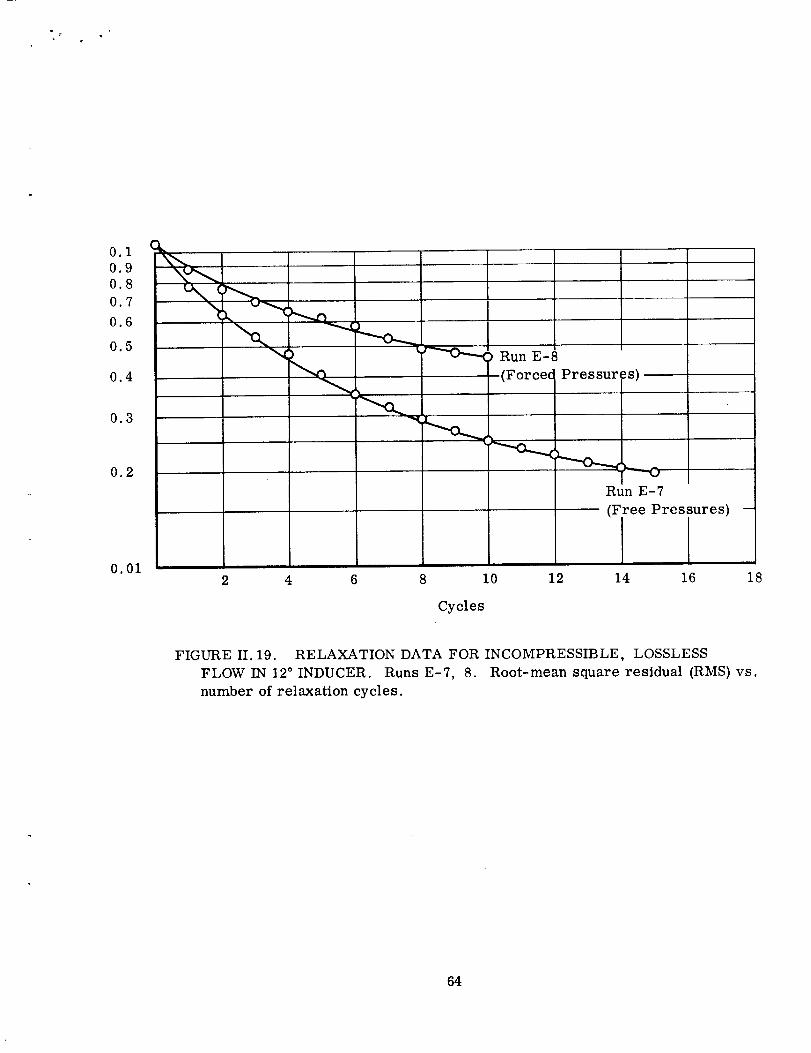
r
0.10,90.8
0.7
0.6
0.5
0.4
0.3
Run E-8
Pressur _s)
0.2
0.01
Run E-7
{Free Pressures)
2 4 6 8 10 12 14 16 18
Cycles
FIGURE II. 19. RELAXATION DATA FOR INCOMPRESSIBLE, LOSSLESS
FLOW IN 12 ° INDUCER. Runs E-7, 8. Root-mean square residual (RMS) vs.
number of relaxation cycles.
64

t4 .
_D
g.,
O
O
1.0
0.9
0.8
0.7
0.6
0.5
0.4
0.3
0.2
/
iI.
O
-O
I I
Run E-8 (Forced Pressures) =o
O Run E- 7
(Free Pressures)
0,1
0o0
0 2 4 6 8 10 12 14 16
Cycles
FIGURE II. 20. CIRCULATION RELAXATION DATA AT EXIT FOR
INCOMPRESSIBLE, LOSSLESS FLOW IN 12 INDUCER.
Runs E-7, 8. Relative circulation ratio ( Fcalc,/F true ) vs.number of relaxation cycles.
65
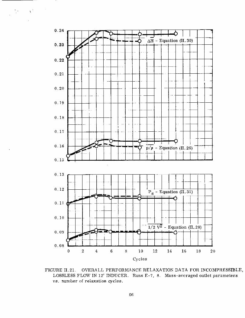
0.24
0.23
0.22
• 7/ - -- -_-- - AH,- Equation (II. 30)
0.21
0.20
0.19
0.18
0.17
0.16_o o "" .... _'--" "(] p/p - Equation (II. 26)
0.13
0.12
O. 11 _
0.10
0.09
0.08
Ps - Equation (II. 31)
-- -8-- ....
0 2 4 6 8 10
--- 1/2 V 2 - Equation (II. 28)
0
12 14 16 18 20
Cycles
FIGURE II. 21. OVERALL PERFORiVLkNCE RELAXATION DATA FOR INCOMPRESSIBLE,
LOSSLESS FLOW IN 12 ° INDUCER. Runs E-7, 8. Mass-averaged outlet parameters
vs. number of relaxation cycles.
66
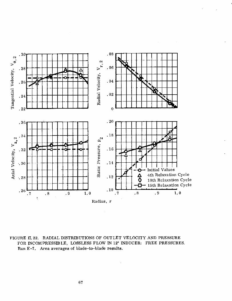
• 3O¢q
28
26
= .24
_ .22
I Ill
1 | .
.O8
>_2 06
o 04
>
_ .02
0
]
.36 ...... .20
.34 _ .18 ,_) _.._
- e= , .16 "- L"
..30 --- _ .14
.. 28 m .12
1• 26 .10
.7 .8 ,9 1.0
Radius, r
_d
,_lllIJill--O-- Initial Values
..fl. _ 4th Relaxation Cycle* 10th Relaxatio: Cycle
15th Relaxatio Cycle|
.7 .8 .9 1.0
FIGURE II. 22. RADIAL DISTRIBUTIONS OF OUTLET VELOCITY AND PRESSURE
FOR INCOMPRESSIBLE, LOSSLESS FLOW IN 12 ° INDUCER: FREE PRESSURES.
Run E-7. Area averages of blade-to-blade results•
67

solutions of inducers. For example, those of reference 6 canbe shownto tend toward free vortex flow: V0 high at the hub and low at the tip.(In subsequentruns we did achieve this. SeeFigures II. 23 and III. 6.)The flow pattern of relative circulation counter to the direction of rotationof the machine, however, was present in the distributions of the relativevelocity components. Part of this may be due to the fact that the circum-ferential distance betweengrid points at the trailing edgeis approximately3/5 of the channelwidth. Another reason may be the fact that the absolutevalue of pressure is inconsequential in satisfying the equations of motion(for an incompressible fluid) andthat only the local pressure gradientsneedbe approximately correct (seeequations (II. 5) through (II. 8). Totest this hypothesis we made the following run for comparison.
Run E-8:12 ° Inducer - 5 x 5 x 22 Grid - Forced Pressures
The geometry and initial assumptions for this run are exactly the sameones as were used for the previous run. During the relaxation procedure,
however, the pressures are forced to satisfy
Pf (r 2 ft 2 u 2 v 2 w 2)p = __ + wl 2 - _ _2g o
(II. 42)
This requirement introduces no mathematical inconsistency, because, for
zero inlet pressure, no inlet whirl, no losses and an incompressible
fluid, equation (II. 42) applies exactly everywhere in the flow field. Each
time one of the relative velocity components is varied at a grid point
(see Section II. A. 3), the corresponding local value of the pressure is
immediately calculated from equation (II. 42). Therefore, Pi, j, k is no
longer an independent discrete variable.
Recalling the discussion of the take-up effect from Section II. B. 2, we
would expect the value of RMS to be higher for this run with forced
pressures than they were for the previous run, since D is lower due to
this elimination of Pi, j, k. This comparison is shown in figure II. 19.
However, figure II. 20 shows that the relative circulation at exit is closer
to the true value when the pressures are forced to satisfy equation H. 42
than when they are free to be adjusted independently. From figure II. 21
we see that the values of shaft power, Ps, and exit velocity head,
V2, are essentially the same for these two comparative runs. The value
2go of the mass-averaged exit pressure head, (p_, settles at 0. 1635
for free pressures and at 0. 1590 for forced pressures. A one-dimensional
calculation with zero deviation predicts a value of 0. 1406 at the root-mean-
square radius, r -- 0. 869, at the blade trailing edge. The most prominent
effect of forcing the pressures to satisfy equation (II. 42) is seen in the hub-
to-tip distribution of V 0 (see figure II. 23). As was mentioned above, thisis the type of distribution we would expect for this problem.
68
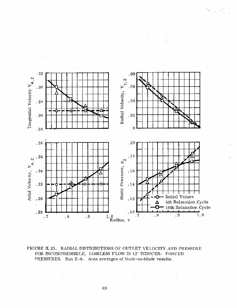
•32¢q
;>_ . 30
24
8 .........
_,1 36
- 34
.28.7 .8 ,9
,2O
,18
g
14 j
.lO.0Radius, r
[ t •
-°-
q_J' J
_" I I I I I I--'O'- Initial Values
4th Relaxation (
--O-- 10th Relaxation1 l I I I I I i n
.7 .8 .9
',ycle
Cycle
1.0
FIGURE H, 23. RADIAL DISTRIBUTIONS OF OUTLET VEI,OCITY AND PRESSURE
FOR INCOMPRESS1-BLE, LOSSLESS FLOW IN 12 ° INDUCER: FORCED
PRESSURES. Run E-8. Area averages of blade-to-blade results.
69
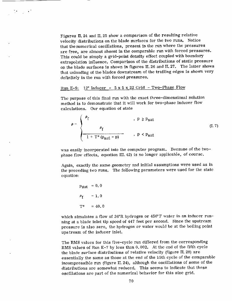
• v • °
Figures II. 24 and II. 25 show a comparison of the resulting relative
velocity distributions on the blade surfaces for the two runs, Notice
that the numerical oscillations, present in the run where the pressures
are free, are almost absent in the comparable run with forced pressures.
This could be simply a grid-point density effect coupled with boundary
extrapolation influence. Comparison of the distributions of static pressureon the blade surfaces is shown in figures II. 26 and II. 27. The latter shows
that unloading of the blades downstream of the trailing edges is shown very
definitely in the run with forced pressures.
Run E-9: 12 ° Inducer - 5 x 5 x 22 Grid - Two-Phase Flow
The purpose of this final run with the exact three-dimensional solutionmethod is to demonstrate that it will work for two-phase inducer flow
calculations. Our equation of state
i Pf , P-> Psat
P= pf
i + T* (Psat - P) ' p < Psat
(I. 7)
was easily incorporated into the computer program. Because of the two-
phase flow effects, equation III. 42) is no longer applicable, of course.
Again, exactly the same geometry and initial assumptions were used as in
the preceding two runs. The following parameters were used for the state
equation:
Pgat = O. 0
pf = 1.0
T* = 40.0
which simulates a flow of 36°R hydrogen or 450°F water in an inducer run-
ning at a blade inlet tip speed of 447 feet per second. Since the upstream
pressure is also zero, the hydrogen or water would be at the boiling point
upstream of the inducer inlet.
The RMS values for this five-cycle run differed from the corresponding
RMS values of Run E-7 by less than 0,002. At the end of the fifth cycle
the blade surface distributions of relative velocity (figure II. 28) are
essentially the same as those at the end of the 15th cycle of the comparable
incompressible run (figure II. 24), although the oscillations of some of the
distributions are somewhat reduced. This seems to indicate that these
oscillations are part of the numerical behavior for this size grid.
7O
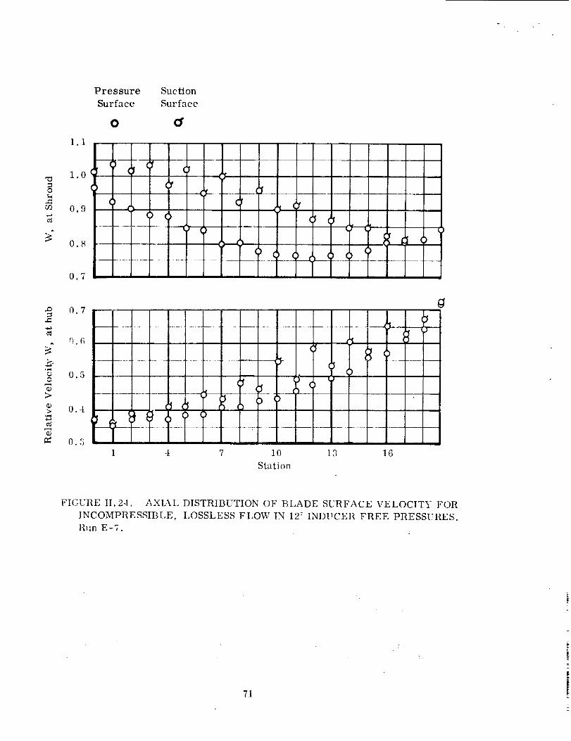
r
0
1.1
1.0
0.9
0.8
0.7
Pressure Suction
Surface Surface
0 cr
(f
() (()
I
I
C
c_
0
o>o;>
c_
o
" 6-; °
0,7 ......... i
.................. .....
I
0.5
0.4
O. 5
c_
1 4 7 10 13 16
Station
g
FIGURE II. 24. AXL&L DISTRIBUTION OF BLADE SURFACE VELOCITY FOR
INCOMPRESSIBLE, LOSSLESS FLOW IN 12' INDUCER FREE PRESSURES.
Run E- 7.
71
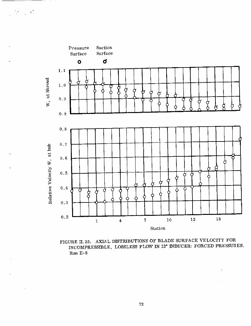
T
-4--*
Pressure Suction
Surface Surface
o
1.0 (_
0.9
0.8 , n i
ITT
• . ,
o
Q
0.8
0.7
0.6
0.5
0.4
0.3
I
!
m
0.2 16
Station
III
|t
(
t
FIGURE II. 25. AXIAL DISTRIBUTIONS OF BLADE SURFACE VELOCITY FOR
INCOMPRESSIBLE, LOSSLESS FLOW IN 12 ° INDUCER: FORCED PRESSURES.
Run E-8
72

w
O
_q
e
•2O
.16
.12
.08
.O4
.00
Pressure
Surface
O
Suction
Surface
C
_r
()
7
f
¢
(
(¢
fr
(
¢p
_f ¢(
?
c_
aD
a_
O
¢0
o_
.20
.16
.12
.08
.04
.00
f
c
c__f
( )"
_fit (
t
c
()
1 4 7 10 13 16
Station
I
(: ci
FIGURE II. 2a. A;_IAL DISTRIBUTION OF BLADE SURFACE PRESSURE FOR
INCOiLPRE_,SIBLE, LOSSLESS FLOW IN 12 INDUCER: FREE PRESSURE.Run E-7.
73
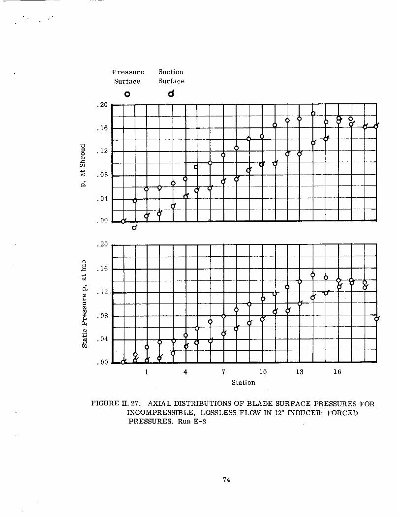
• ¢ i, "
o=
.2O
.16
.O4
O0
2O
Pressure
Surface
0
(
LJ
¢f
Suction
Surface
d
,,_f' r,,
) ( L
(m
C
(f
r (
(
I I I
q.)
¢,..)°i,-.4
16
12.
O8
04
O0 r¢
I
_ _r Ir
1
_c
( 0 L
) , (f'
(( fr
i
4 7 10 13 16
Station
FIGURE II. 27. AXIAL DISTRIBUTIONS OF BLADE SURFACE PRESSURES FOR
INCOMPRESSIBLE, LOSSLESS FLOW IN 12 ° INDUCER: FORCED
PRESSURES. Run E-8
74

-T
0
v$
1.1
1.0
0.9
0.8
0.7
Pressure
Surface
O
f $ _e
,gg
Suction
Surface
d
(f
()
_f
(_()
C
c_
"1 _' sf
,.Q
-F--t
¢90
;>
>
0.8
0.7
0.6
0.5
0.4
0.3
(
? (..s
I
1 4 7 10 13 16
Station
FIGURE II.28. RELATIVE VELOCITIES (W) ALONG BLADES OF 12 °
INDUCER CItANNEL FOR HOMOGENEOUS TWO-PHASE, LOSSLESS
FLOW: Run E-9.
75
w
Because the upstream stagnation surfaces, as we have selected and fixed them,
actually do work on the fluid, by the time the fluid reaches the blade leading edge
its pressure is already above saturation pressure. This is where the selection of
proper stagnation surfaces is crucial. The internal density distributions indicate
vapor in the flow region upstream of the blade leading edge. This vaporous region is
small compared to the entire flow passage. For a value of T*= 40.0 and an inlet
pressure equal to vapor pressure, we would expect a large portion of the passage to
fill with vapor (see table III. 1 and figure HI. 24}. The apparent unloading of the
blades, especially at the tip, is due to the fact that figure II. 26 shows the results of
15 relaxation cycles whereas in figure II. 29 are shown the results of only five cycles -
i.e. the solution has not been carried far enough to give the correct answers. The
rotational flow pattern for both the two-phase and the incompressible run are es-
sentially the same. All hub-to-tip distributions at the blade trailing edge, for example,
differ from each other by less than 0. 001.
76

•2O
.18
.O4
•O0
Pressure SuctionSurface Surface
o d
1 l$
_r _ cY
c_
c_
t_8__9
;h_9
.12
.08 ¢
_ T_'.04
,,f..
(
,r
A
c ' J
(j'
1 4 7 i0 13 16
I_c
I_r c
r
Station
FIGURE n.29. AXIAL DISTRIBUTIONS OF BLADE SURFACE PRESSURE FOR
TWO-PHASE, LOSSLESS FLOW IN 12 ° INDUCER: Run E-9.
77

C. CONCLUDINGREMARKS ON EXACT METHOD OF SOLUTION
The foregoing sequence of examples demonstrates the capabilities of our numerical
approach to an exact method for obtaining three-dimensional solutions of general,continuum fluid flows in turbomachinery. That the method gives valid answers is
empirically evident as we now review the results of these examples.
1. Review of Problems Solved
The paddle-wheel channel examples with lossless, wheel-type flow indicate that a
convergent solution is always possible -- the resulting root-mean-square (RMS)
residual for the incompressible case (run E-l) being much less than one percent.
While this capability for minimizing the RMS residual is borne out by all the other
examples, run E-2 (similar to E-l) illustrates it best by producing an answer of
1/10 of one percent, with no sign that this is remotely close the attainable minimum
(Figure II. 7). Furthermore, run E-2 shows that two-phase flow effects can be in-
cluded successfully -- and with no perceptible increase in computing time. Finally,
these two simple examples illustrate the deviations from the true answers that are
caused by discretization, i.e. by a finite number of grid points (3 x 3 x 3). Even
though the system of finite difference equations and other conditions can essentially
be satisfied in this special case, the solution to the comparable continuous problem
(infinite number of grid points) yields a different radial distribution of the pressure.
The three examples (runs E-3, 4, 5) of incompressible, irrotational flow in a paddle-
wheel channel illustrate the grid effects of typical problems. Here we observe the
numerical inconsistency of the (essentially arbitrary) linear extrapolations at boundary
points with the more complicated pressure and velocity variations there; i. e., the
RMS residual achieves a minimum (or nearly so) that is non-zero in each case. Even
though this residual is far enough from zero (Figure H. 9) for completely wrong answers
to be allowable by it, the results are fairly accurate (Figure II. 10). In fact, the
experiments that we conducted in runs E-4 and E-5 wherein we changed the problem of
run E-3 by extending the number of points and unknowns (without altering grid point
density) shows that a lower residual does not guarantee more accurate answers,
(unless it is sufficiently low): The additional adjustment of variables that was possiblein runs E-4 and E-5 illustrates this "take-up effect".
The foregoing discretization error is probably not dominant in runs E-3, 4 and 5, because
the cross-sectional density of grid points is about seven times greater than was the case
in runs E-1 and 2, (9 x 7 versus 3 x 3). The answers were acceptable -- even with the
relatively high RMS residual results. We used approximately correct values as initial
assumptions, and starting with this lack of bias is probably the way to obtain reasonable
results when the minimum obtainable RMS residual is not low enough to guarantee
them. The numerical inconsistencies responsible for this inability to obtain such
a minimum would be less dominant for a greater density of grid points.
78
The sample inducer examples that we studied in runs E-6 through 9 had no parallelsets of previously knownanswers by which the results could be judged directly --as was possible with all the other cases. However, results for similar geometriesusing acceptedsimple radial equilibrium methods, (as was donein reference 6, andby us in Section III,) give an indication of what to expect. The 5 x 5 grid point cross-section with the many additional points obtained by reason of the greater channellength {up to 22 cross-sections) typical of inducers, yield the kind of answers thatwould be expectedfrom our knowledgeof the irrotational flow results for the paddle-wheel channel, (runs E-3, 4, 5). These inducer problems yield minimum RMS residualsof order similar to that of runs E-3, 4, 5. (cf. Figures II-9, 13, 19). Although thegrid-point cross-section is 5 x 5, (vs. 9 x 7 for runs E-3, 4, 5) the channel inclinationangle is quite shallow andyields the higher grid-point density that probably accountsfor the differences betweenthe inducers andthe paddle-wheel channel.
However, a greater grid point density is neededto avoid the further numerical errorsthat were probably introduced by using the convenient arrangement with highly obliqueintersections of the coordinate surfaces, (Figure A-2). This results from the factthat inducer channels are inclined at sucha low angleBto the tangential direction.
The foregoing conclusions about the take-up effect apply to the differences between the12° inducer results for free vs. forced pressures, (runs E-7 vs. E-8). The latterproblem had fewer unknownsand thereby accountsfor the higher RMS residual,(Figure II-19). Here again, these residuals were high enoughin both cases to allowwrong answers, but the forced-pressure case seems to have insured reasonably accurateanswers. In effect, biasing the pressures toward results that are consistent with thevelocities reduces the grid-point density that is required; however, it restricts theproblem to the lossless case -- which is what we solved in all our exampleswith themethod.
Finally, we could have obtained more accurate answers in the inducer examples if wehad adjusted the initially estimated upstream anddownstream extensions of the bladesto unloadedpositions as the solutions proceeded. The errors that we introduced by notdoing this are probably small compared to those that are causedby the coarse-grideffects. However, the two-phase flow results of run E-9 are influenced by the fact thatthe slight loading that did occur on the upstream stagnation stream surfaces preventedvapor from forming in the locations where its effects are knownto be most pronounced.Here againwe have demonstrated that two-phase flow calculations introduce no significantchanges in computing time and complexity.
2. Recommendations for Future Work
Since the numerical accuracy of this exact method appears to have a direct relationship
with the density of grid points, one must provide the attendant necessary computer
storage space and running time to reduce the residuals sufficiently, (see Appendix C).
This is characteristic of any valid finite difference technique.
79

A review of the data that we obtained in checking the method indicates that in its presentform the program (AppendixC) would probably give satisfactory results if onewouldapply it to any typical inducer channel as follows..
a) Use a grid of 10x 10 x 50 points, which compares to 5 x 5 x 22 thatwe used.
b) Extend the stagnation stream surface boundaries about one channelwidth upstream and downstreamas we did it runs E-7, 8, 9.
e) Adjust the locations of these surfaces after each set of ten relaxation
cycles to maintain them in an unloaded condition; i. e., there should
be no pressure differences across them at the same radial and axial
locations.
d) Change the subroutine ADJ (Appendix C) to force the pressures to
satisfy equation H. 42 as we did in run E-8. This eliminates thetreatment of losses in detail; however, other expressions similar to
equation II. 42 can be devised to distribute losses arbitrarily and to
handle two-phase flow in combination with the barotropic relation
(equation I. 7) -- subject to the inlet conditions of uniform pressure andzero whirl.
As here proposed, the problem may yield a satisfactory solution in less than twenty-
five relaxation cycles at a cost of about one half hour of computing time per cycle,
(see Univac 1107 data in Appendix C). Proposal (d) on "forcing" the pressures may
not be necessary if more computing time is allowed. It is simply a way of keeping
the problem within present limits of computer storage and calculation times, as the
general case would require even more grid points than 10 x 10 x 50 for an accuratesolution.
Further work on the method itself could yield the reductions in calculation time that
would allow the use of finer grids with the general problem (pressures not forced)
on existing computers. A method for automatically adjusting the stagnation stream
surfaces would save the time required to do it by hand in (c) above. As concerns the
computational algorithm itself, lower RMS residual values could be attained by treating
the wall boundary conditions (equation II. 9) as additional residuals and by independently
adjusting all velocity components at boundary points, (see Appendix A).
More advanced residual reduction techniques could be introduced to accelerate the
convergence rate, which might be partly accomplished with the existing program
by a judicious selection of weights to be assigned to the various residuals at each
grid point. As in the case of all developments and modifications in this method, such
improvements would require the closest cooperation between the fields of numerical
mathematics and fluid dynamics.
8O


SECTIONIII
APPROXIMATE THREE-DIMENSIONAL SOLUTION
A. METHOD OF SOLUTION
This section gives the assumptions and method for obtaining a rapid, approximate
solution to the system of equations and boundary conditions presented in Section i,
The resulting program (Appendix D) can obtain answers in about a minute on existing
computers and may therefore be used for purposes of assisting in design evaluations.
However, such answers cannot describe the detailed three- dimensional flow patterns
that include, e.g., blade loading at the leading and trailing edges and relative cork-screw motion within the passages. Any basic study of the inducer flow field must
be made by the exact method of the preceeding section.
The philosophy for this approximate approach is primarily that of reference 1 in thatseveral assumed two-dimensional solutions of the blade-to-blade field are coupled
with a complementary two-dimensional meridional solution. As reasonable approxi-
mations for inducers, we have neglected the effects of streamline curvature in the
meridional plane and of blade forces normal to the streamlines in that plane. Also
presented is the form of the results which can be correlated with other theoretical or
experimental data.
1. Restrictions of the Analysis
We imposed the following restrictions on the fluid motion to obtain an approximate
solution:
a) The fluid flows through the inducer (figure HI. 1) in annuli; i. e., in the
spaces between stream surfaces of revolution formed by rotating aboutthe axis of rotation the meridional projections of the streamlines of such
a flow. (Unless otherwise noted, the term streamlines will hereafter refer
to these projections. )
b) The stream surfaces have initially fixed locations at the leading edge of
the inducer blade (figure III. 1, view b). The upstream set of boundary
conditions is applied at that leading edge, thus precluding backflow.
c) Average relative velocity and pressure conditions exist at mid-passagefrom blade to blade, (see figure II. 2). These averages are results of the
meridional solution, and they are the quantities employed (with additional
assumptions) to determine the blade-to-blade solutions. Where two-phase
flow exists, we allow the meridional and blade-to-blade solutions to be
dependent on one another.
d) The direction of the average relative velocity in a given annulus differsfrom that of the blade meanline in the blade-to-blade plane (figure III. 2)
81

0
82
\
0
A
\
Z0
0r._
0
' 0
N©
©
r..)
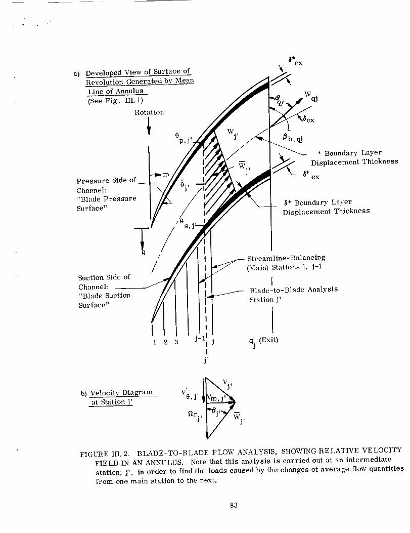
a)
ex
Line of Annulus
(See Fig.
D:::ll:tP;: n VG::er°_t_drbfycM ea°fn /__
W .III.I)
_ ._,_ox
'
Pressure Side of
Channel:
"Blade Pressure
Surface"
T//!Suction Side of / j
C_a_ne_:------_//"Blade Suction //
1 2 3
* Boundary Layer
Displacement Thickness
$* Boundary Layer
Displacement Thickness
I
I-i
J II
•_1 IIIj,
Streamline-Balancing
_-- (Main) Stations j, j-1
i_/- Blade-to-Blade Analysis
Station j'
qj (Exit)
b) Velocity Diagram
at Station ]'
V°,
VO, j' , ]__9rj,
j,
FIGURE IH. 2. BLADE-TO-BLADE FLOW ANALYSIS, SHOWING RELATIVE VELOCITY
FIELD IN AN ANNULUS. Note that this analysis is carried out at an intermediate
station; j', in order to find the loads caused by the changes of average flow quantities
from one main station to the next.
83

by a predetermined deviation angle. In order to close the relative velocitydiagrams at exit, this angle is assumedto vary approximately with thesixth power of length from the zero inlet value to the imposed exit value onthat annulus. The componentof direction in the meridional plane is thatof the mean line betweenthe two boundingstreamlines {figure IH. 1).
The task is to find the equilibrium locations of the streamlines along each of severalfixed straight-line meridional quasi-normals in turn at successive stations from inletto outlet. At station 1, the blade leading edge, no suchbalance is required, as thelocations there are fixed by restriction (b).
Although the relative corkscrew motion that can occur in a real flow is precluded byrestriction (a), Stanitz showed(reference 12) that this superimposedmotion has littleeffect on the velocities and pressures of an essentially single-phase lossless flow inthe interior of the machine. Furthermore, we foundthat the total amount of thisrelative rotation experiencedby the internal fluid seldom exceedsone-half turnbecauseof the low work level of inducers. Finally, at low NPSH, the inlet region ofan inducer commonly unloads due to two-phase effects, which would then makerestriction (a) more acceptablethere.
For the low blade-to-blade loadings of inducers, restrictions (c) and (d) shouldbereasonable. The deviation angle distribution of (d) amountsto negligible deviationexcept in the latter third of the blading, if imposed. In this way, the blade exit unloadingphenomenoncan be approximately simulated.
This reasoning simply meansthat our approximate solution ought to give a fair indicationof inducer performance. However the three-dimensional (exact)method employs noneof these restrictions; and, when applied with sufficient accuracy, it is the ultimatestandard for a final design. Furthermore, basic observationsof loss distributions andtheir effects canbe understood best in the light of an exact solution -- even one of alossless flow.
2. Scalar Equations and Boundary Conditions
The foregoing restrictions lead to a natural set of varying directions in which to apply
the equations of motion, using the (r, 0, z) right circular cylindrical coordinate system(figures HI. 1, 2):
a) The relative flow direction h, which is that of the foregoing restriction (d).
b) The direction of the straight-line meridional quasi-normal n'.
c) The tangential or blade-to-blade direction 0.
It is in these directions that we now express the three component equations of the vector
momentum equation (I. 2 or I. 4). Since his the relative stl_eamline direction, we use
the streamline momentum equation (I. 12) of Section I. A. 2:
84

godp(02r2)- d -d - dL (m. 1)p 2
In the n' direction, we have the following simple normal equilibrium equation:
1
go dp VO2 cos_ (HI 2)
p dn' r
and in the 0 direction, we use the moment of momentum equation in terms of the average
velocities and blade surface pressures, (reference 3, Appendix; and reference 15,
p. 287):
go Pp - Ps d(r V0) (HI. 3)p 0s _ _p= Vm dm
Note that equation IH. 3 is an integrated form of the scalar momentum equation in the
0 direction (equation II. 2), which is
d (r VO) (III. 3a)0P_ P Vm d--_O0 go
We require continuity throughout each annulus as follows:
dw= d[prAn (0s- 0p) _b Vm] =0(III. 4)
Together with boundary conditions and equations (I. 7) and (I. 13) for two-phase flow and
loss effects when required, equations (III. 1,2, 3, 4) constitute the complete set of
relations used in this method.
We note that equation (IH. 2) is obtained from the complete normal equilibrium equation
for this annulus-type flow problem (reference 4, p. 29):
VO2 V_ 2 + _B* d (rV0)go 0P _ cos_ --_7mO 0n r r c r dm
Pressure Centrifugal Streamline Blade Force
Gradient Action Curvature
(III. 5)
where
* 00 00B= r-_ sin _' - r _ cos_ (HI. 6)
85
Furthermore, (see figure HI. 1)
dp 0 P dn 0 P dm-- +
dn' On dn' 0m tin' (HI. 7)
If the quasi-normals are approximately perpendicular to the streamlines, we see that
the last term of equation (HI. 7) may be neglected and that dp ,._ dp Omitting the"5"-2-_,_dn "
effects of meridional streamline curvature and of the bladed_orces only in the quasi-
normal direction; i.e., the last two terms of equation (HI. 5), we then obtain the simple
normal equilibrium equation (III. 2). Provided we take the care to specify the (fixed)
locations of the quasi-normals properly, the fairly axial, long, straight meridional fields
and nearly radial-element-blades of inducers should make this omission of terms lessserious.
In accordance with the restriction in Section II. A. 1, we summarize the boundaryconditions on this problem as follows:
a) The wall boundaries (Section I. B. 1) extend only from the blade leading to
trailing edge. Beside the blades, hub and shroud, these also include the
stream surfaces of revolution (streamlines), whose locations are fixed at
the upstream boundary.
b) The upstream throughflow boundary (Section I. B. 2) is at the blade leading
edge. There we specify for each annulus the respective inlet values of p,
V m and V0. The direction of Vm is determined by the given slope of theblade leading edge (not necessarily a straight line in the meridional plane);
therefore, Vr and V_ are implicitly specified. No tangential variation ofthese quantities is assumed.
c) At the downstream throughflow boundary (the blade trailing edge), we
specify the respective predetermined values of the tangential averageexit deviation angle Sex for each annulus. The exact locations of these
annuli result from the solution; however their positions can be estimated
closely enough to find the necessary values of _ex if its distribution from
hub to shroud is not uniform. The program as presently constructed
requires that a quasi-normal coincide with the blade trailing edge, and
therefore, that this edge be a straight line in the meridional plane.
3. Meridional Streamline Balancing Procedure
Determining the equilibrium positions of the meridional stream surfaces of revolution
chosen at inlet is the object of this approximate method. We identify the coordinates
of each streamline by the index (subscript) i where
86

.°
1 < i < qi
Hub Shroud
Similarly, each quasi-normal is identifiedby the index (subscript)j (theStation number)
where
1 < j < qj
Blade Blade
Leading Trailing
Edge Edge
All fluid variables (p, p, W, V) are associated with annuli, not the streamlines;
i. e., they are assumed to exist on the mean line of annulus i' which lies midway
between streamlines i and i + 1. Thus the total number of annuli is qi - 1. The
same identification applies to the average coordinate quantities n'i', j, (with
corresponding ri', j, and _i', j, ) which locate the mean line of annulus i'. Thecomputational procedure begins from the specified data by calculating the mass flow
rates w i, and relative velocities Wi', j, for each annulus i' at the blade leading edge
station (j = 1). We then proceed as follows at station 2 (j = 2):
a) We estimate the streamline positions n'i, j, , ri, j and _i, j on the
quasi-normal j by assuming the same spacing proportions as at
j - 1. Next we find the corresponding channel angle data 0s, i', j and 0p, i ', jfrom a blade subroutine for the given blade shape and thickness,
which includes boundary tayer displacement thickness. From this
and similar data at stations j - 1 and j + 1, we obtain the relative
flow angle Bi', j in the plane tangent to the mean stream surface ofeach annulus i', allowing for deviation, if any, (see figure III.2).
b) Applying the continuity equation (Ill. 4) in finite-difference form we
obtain the average velocities Vm,i, ' j as follows:
V wi'm, i',j =
pr An (0 s - Op) ] i',j
(III. 8)
With the angles f_ we now obtain also the velocities V 0 and W. If weare not restricted to an incompressible analysis, this and the following
step are coupled to the blade-to-blade solution in the portions of the
machine where vaporization occurs. In such a case, the value of
P i', j is unknown and must be found from an iteration of equations HI. 8
and III. 9 with steps (a) through (f) of the blade-to-blade solution for two-
phase flow, (see Section HI. A. 4).
87
c) Next we obtain the averagepressures Pi', j from the streamline momentum
(equation (HI. 1)) expressed in finite-difference form:
Pi',j = Pj_I 2g o -2- rJ 2 _ rj-12 1+ _ j2 _ Wj_I - dL (HI. 9)
i'
d)
where dL is similarly expressed by finite-difference forms of equations
(I.13, i4, i5).
Now we form the streamline unbalances Ui, j for all i from the
normal equilibrium equation (III. 2), (i = i):
U. = Pi' - Pi'-i _ (Pi' +Pi'-l) @,iZ + V_,i' - 1 (III. lO)
l, j n'i' - n'i' -1 4go ri/cos 7'
where no U's are needed for the hub and shroud streamlines (i = 1 and
qi respectively). These indicate the extent of error in the original
estimates of the streamline positions in step (a).
In the following steps, we adjust the streamline locations n'i, j at stationj to satisfy the same accuracy criterion developed in Section II. A. 4.
Here, we require (similar to relation (II. 19) that the unbalance U belimited as follows:
Pf
U < _ (l_ 2 rt) g---_-
where _ is some small number.
The relation of this error to the overall results is less serious than the
discussion of Section II. A. 4 would indicate. It affects the hub-to-shroud
distributions, but not the accuracy of the inlet-to-outlet annulus results in
themselves. Continuity is satisfied in each annulus, and the correct pressure
rise from inlet to outlet of it will result if on the average each annulus is
balanced with relation to the others. Any cumulative effect due to bias in
the unbalances is small, and in the lossless case it is non-existent -- the
overall pressure rise error then depending on bias in the unbalances (due
to _0) at the exit station only. Note that "unbalance" U is an error ind__p_,the normal pressure gradient (i. e. _r in typical inducers).dn t
The adjustment sequence at station j follows:
e) If all the Ui, j satisfy condition (IH. 11), we consider the problem solvedfrom the inlet to this station j. In such a case, we proceed to the next
(Ill. 11)
88
station (j + 1) and repeat the steps just outlined, beginning with step (a).If, however, this required accuracy doesnot exist, we execute the followingsteps starting with streamline i = 2 at station j:
We determine a new streamline position (n' + An'h, j by the second order
Taylor approximation, (see equation (II. 17)):
n n=n 0n,---y/(HI. 12)
where the U derivatives are evaluated by moving the streamline by
amounts ± _n' and executing ste_s (b) through (d) for each such movement.
In the event that the U versus n' relation is not sufficiently second order
for the adjustment given by equation (HI. 12) to cause a reduction in Ui, j,
we accept whichever result of the + _n' calculations did cause a reduction,
if indeed one occurred. (This alternate method was necessary in the two-
phase flow cases. It does not force a wrong answer but merely insuresthat the unbalance U will be reduced in cases where the usual method cannot
accomplish this.) If required to obtain U reduction, $n' is reduced as in
the method of successive variations (Section H. A. 3) at the end of each
cycle.
g) We repeat step (f) for the next streamline, i = 3, and so on through i = qi - 1,
which completes one (hub-to-shroud) iteration cycle. Then we return to
step (e).
In certain cases where a very small value of • in equation III. 11 would
require may iteration cycles, the number of cycles can be limited and the
results accepted at the accuracy then achieved, (see Appendix D).
4. Blade-To-Blade Solution
Except for cases where pressures in the blade-to-blade solution are lower than the
vapor pressure Psat, there is no influence of this solution on the meridional one of
the foregoing section. For two-phase solutions, we make a blade-to-blade check for
vaporization each time an average density Pi', j is required by steps (b) and (c) ofthat section. The blade-to-blade solution associated with a given station j is actually
carried out at j' which is halfway between j and j - 1, (see figure III. 2). The results
are the fluid relative velocities Wp, i',j' and Ws, i',j', pressures pp, i',j' and Ps, i', j',
and densities pp, i', j', and Ps, i', j' on the pressure and suction sides of the channel,respectively.
The meridional field does of course determine the blade-to-blade solution, and the
key to this is the moment of momentum equation (III. 3). To use simply this equation
two assumptions are required; viz., a 0 distribution of one of the variables and.astatement about the accumulated losses versus 0. For the first, a linear distribution
p(0) (reference 2) or W(0) (reference 1) is generally assumed. Both of these give
89

nearly the sameresults for the light loads in the incompressible case. However, inthe two-phase case the linear pressure approach causesunrealistically high W's onthe non-liquid suction side of the channelbesides specifying anappreciable pressurevariation over a region that is essentially vaporous (reference 8, p. 4-16). Sowechose the linear velocity model, which best fits all cases. For the secondassumption,the only convenient approach is to state that fidL along all relative streamlines in
annulus i from inlet to station j' is uniform. Then the streamline momentum equation
(I. 12) holds on all streamlines from blade to blade (r = constant), and it may be em-
ployed together with the state equation (I. 7) to relate the 0 distributions of the variables
p, W and p.
Having chosen the linear velocity model, we next obtain the relationship between W(0)
and the velocities of the meridional solution which are averages. As in reference 1,we assume
W +W )s p = Wi',j' (HI.13)2i',j'
The average velocity
W.+ )J Wj-1 (HI. 14)
Wi',J ' = 2 i'
does the pressure, Pi' "' lies at mid-passage, where _ is defined similarly. Inas,J
accordance with the foregoing assumption about the losses, we now combine the moment
of momentum equation (IH. 3) with the following form of equation (I. 2) for use in the 0
direction (r = constant):
go dp- W d W (Ill. 15)
p
Assuming
PP- Ps dp
0 s - Op dO(HI. 17)
we obtain
-_-] j, mj - mj_ 1T, !
i'
(III. 18)
9O
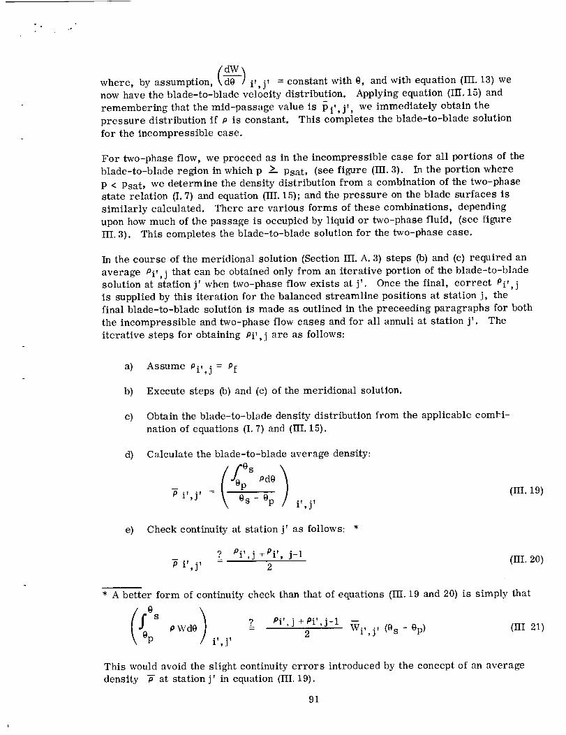
where, by assumption, i', j' = constant with 0, and with equation (III. 13) wenow have the blade-to-blade velocity distribution. Applying equation (III. 15) and
remembering that the mid-passage value is p i', J', we immediately obtain the
pressure distribution if p is constant. This completes the blade-to-blade solution
for the incompressible case.
For two-phase flow, we proceed as in the incompressible case for all portions of the
blade-to-blade region in which p > Psat, (see figure (HI. 3). In the portion where
P < Psat, we determine the density distribution from a combination of the two-phase
state relation (I. 7) and equation (IH. 15); and the pressure on the blade surfaces is
similarly calculated. There are various forms of these combinations, depending
upon how much of the passage is occupied by liquid or two-phase fluid, (see figure
HI. 3). This completes the blade-to-blade solution for the two-phase case.
In the course of the meridional solution (Section III. A. 3) steps (b) and (c) required an
average Pi', j that can be obtained only from an iterative portion of the blade-to-bladesolution at station j' when two-phase flow exists at j'. Once the final, correct Pi',j
is supplied by this iteration for the balanced streamline positions at station j, thefinal blade-to-blade solution is made as outlined in the preceeding paragraphs for both
the incompressible and two-phase flow cases and for all annuli at station j' The
iterative steps for obtaining Pi', j are as follows:
a)
b)
c)
d)
Assume Oi,,j = Of
Execute steps (b) and (c) of the meridional solution.
Obtain the blade-to-blade density distribution from the applicable comki-
nation of equations (I. 7) and (HI. 15).
Calculate the blade-to-blade average density:
e) Check continuity at station j' as follows: *
(HI. 19)
=? Pi',j +Pi', j-1 (III. 20)"Pi',j' 2
* A better form of continuity check than that of equations (III. 19 and 20) is simply that
s ? Pi',j+Pi',j-I Wi',j' (Os - Op) (HI 21)p Wd0 '- 2Op i',j'
This would avoid the slight continuity errors introduced by the concept of an average
density "_ at station j' in equation (III. 19).
91

°.
Pp
Density
P
Wp
Relativ_______e
VelocityW
Pressure
P
Pf
pp II
II
Liquid _ Two-Flow _ Phase
] FlowI
I
op 0sat
Psat
P
Central Angle, 9
WS
PS
Ps
0 s
FIGURE HI. 3. BLADE-TO-BLADE DISTRIBUTIONS OF FLUID FLOW
VARIABLES. At station j' (between stations j and j-1 see Fig. III. 2).
92

• F
0 If the difference between these averages is greater than. 001 of the
right hand side, we reduce Pi', j by a small amount and repeat steps(b) through if). If the difference is less than. 001, we accept the current
value of Pi',j for use with the meridional solution, (steps (b) and (c)).
Figure III. 4 shows the kind of variation that results for each side of equation (HI. 20)
as the assumed average density Pi',j is changed from Pf to successively lower values.The iteration procedure contains safeguards to avoid the solution bb (figure III. 4) for
negative blade loading and to handle properly the choked annulus case for which no
solution exists. First, if solution aa exists, it will be reached first as the blades unload
with decreasing values of the assumed Pi', j. We found that if no solution aa exists,there will be no bb solution either, since a negative blade loading causes a reduction
of average pressure from station j - 1 to j with corresponding increased vaporization.
So, if no solution exists; i. e., if the annulus is choked for current positions of the two
bounding streamlines, this fact is noted by the computer, andwe use the value of Pi v, j
for essentially zero blade loading (specifically, the value obtained at the point in the
iteration for which V 0 = 0) in steps (b) and (c) of Section IH. A. 3. If the streamline
adjustment sequence ultimately yields no balanced positions of the streamlines at
station j (steps (e), (f) and (g) of Section HI. A. 3) for which all the annuli are unchoked
at j'; an appropriate message is printed at the end of a maximum allowable number of
balancing cycles, and the calculations are discontinued.
5. Form of the Results
The procedures for obtaining the meridional and blade-to-blade solutions yield sets of
hub-to-shroud results at each station j and at jr; i. e., respectively along and between
the quasi-normals of the meridional solution from inlet to outlet. At j we give the
resulting set of streamline coordinate locations r and _ and the final unbalances U.
The set of average annulus values W, Vm, Vr, V 0, V_, p and pare each also given
for j. At j', we give the blade-to-blade results for each annulusat the blade surfaces
and at mid-passage; viz., Wp, Ws, W, pp, Ps, _, PP, Ps; and _, which does not lieat mid-passage, (see figure III. 3) and equation (III. 19)).
At the blade trailing edge (j = qi) we also calculate blade element performance data and
finally the overall performance of the machine. The blade element data applies to fluidin each annulus and is calculated as follows:
a) Total head loss coefficient:
I / 2 1 2v02 1v01 p2 plgo go P2 P1 2 go 2 go /
= 2
wt, 1 / (2 go)
(III. 22)
93
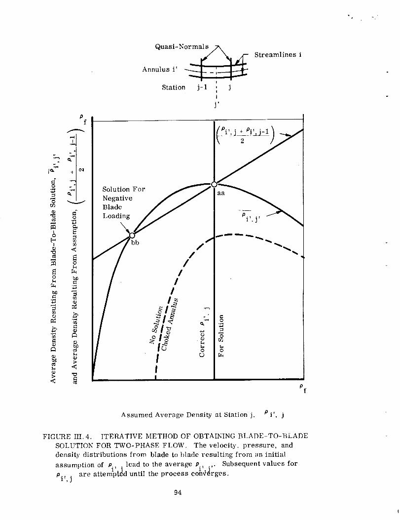
O
o
I
0
I
o
o
N;
<
pf
I°_.._
+
0.r..44_
<
0
o
o>
<
Quasi-N_Annulus i'
I
Station j-1 , jI
I
j,
Streamlines i
Solution For
NegativeBlade
Loading
///
II
aa
Pi'. j'
Pf
Assumed Average Density at Station j. P i', j
FIGURE III. 4. ITERATIVE METHOD OF OBTAINING BLADE-TO-BLADE
SOLUTION FOR TWO-PHASE FLOW. The velocity, pressure, and
densits' distributions from blade to blade resulting from an initial
assumption of P , lead to the average p , , Subsequent values fori ' i,"
Pi', j are attempted until the process converges.
94
b) Annulus efficiency:
_i' = p_ _1 v_ Vl_)P2 Pl + 2go 2go
U2 V0, 2 U1 V0, 1
go go i T
(IH. 23)
The overall performance is calculated from the proper averages of the
annulus (i') data at inlet and outlet:
a) Mass flow rate:
qi -1
w T = i__l_ w i (III.24)
b)
where the w i are given by equation HI. 4 for use in the programcalculations.
Mass-averaged total head rise
qi- 1 V2
E (_ _+i'=l P-2 Pl 2goAH =
VI2 )i'2go
w T
w i ,(III. 25)
c) Mass-averaged pressure (calculated at inlet and at outlet):
qi-1
E Pi'wi'i'=lm
p=
w T
(III. 26)
d) Mass-averaged absolute velocity head calculated (at inlet and at
outlet): qi- 1
Z (Vm +VOW)i'i=l 2go
2gow T
(HI. 27)
95

_t _ v
e) Torque:qi-i
Tq- 1 Zgo i=1
(r2 V0, 2 - rl V0, 1)i'w i , (III. 28)
f) Shaft power input:
Ps = l} Tq (III. 29)
g) Overall efficiency:
w
qi-1 2 2
i,_l (P2 Pl + V2 VI t"= _2 Pl 2go 2go i'wi'
Ps
(m. 30)
Observe that the overall efficiency -_ is equivalent to an energy average
of the elemental efficiencies _i,.
B. EXAMPLES AND RESULTS
The approximate method was used to solve a series of problems on the same variable-
lead inducers to which we applied the exact method in Section HI. B. 3. This section
presents the results for the 6.2 ° and 12 ° inducers - which are described in figures II. 12
and II. 18, respectively - for (1) incompressible, lossless flow, and (2) other runs with
loss and two-phase flow. In table III. 1 we list the representative runs reported in this
section; although we made some additional runs to obtain more data for the conclusions
of Section IV. As in Section II. B we performed all calculations nondimensionally,
according to the system presented at the end of the list of symbols.
1. Incompressible Results and Correlations for Lossless Flow
We now compare the results of the approximate method of solution with those of the
exact method, {Runs numbered A and E, respectively), using the following data fromtable III. 1:
a) 6.2 ° Inducer:
Runs A-1 and E-6
Figures III, 5, 7, 8
96

©
Z
o
8
C_
E-wZ
C_
PQ
2_Q
C_
©
C_ c_
r_ _ "I
g
_ Pr ,g
@,
z d ,
oi i
Z', Z
_ N
888
cc
_ o
• . o
t¢3 u'3 _I/3 t_ i/3
t'-- t_ t-,-
0 C) u'3
l l l
,1,
t" ° "
I"
°%%%
_o
I I I i
<<._____<<
8888
Z
g-
I 1 I I
_.'_
d N
• , o
• ° ,
_-t _-t ,--I
L_'. t._ _,1
X X
I I t
op _
aN
I
I
8 _
o %
--_,'0
"H.
_-_ 0(3
II II
c,l
z _O "_
O
×._ _
97

i r
b) 12 ° Inducer:
Runs A-10, E-7 and E-8
Figures III. 6, 9, 10, 11, 12, 13
On each inducer, we used an 8 x 16 field; i. e., one with eight stream-
lines including hub and shroud, and sixteen stations including the blade
leading and trailing edges. Because of the special geometry we used
equally-spaced radial lines for the quasi-normals at each station. The
eight streamlines were equally spaced at station 1. Refer to figures II. 12
and II. 18 for geometrical details, including the axial locations of the
stations.
The overall performance data also appears in table III. 1 in terms of the static pressure
rise coefficient _I,p, total head rise coefficient _I,, power coefficient Ps and overallefficiency -_ . These are the non-dimensional values of the corresponding quantities
presented in Section HI. A. 5. The corresponding data for the exact methods of solution
of these two inducers is also given (from figures II. 15 and II. 21). We obtained a fairly
close correlation of these results and the approximate ones {Run A-10) for the 12 °
inducer. Lack of such a correlation for the 6.2 ° inducer is probably the result of a
7% error in the fixed outlet throughflow velocity distribution that we made in applying
the exact method, (see description of Run E-6 in Section II. B. 3).
This difference is more clearly shown in the radial distributions of velocity and
pressure at the blade trailing edge in figure III. 5, especially for the Vz component,which distribution was fixed in Run E-6. The unusual V0 distribution of run E-6
isprobably due to the grid effect. Figure III. 6 for the 12 ° inducers shows close cor-relations bet_veen Runs A-10 and E-8, the latter being the forced-pressure case of the
exact method, (see theRun E-8 discussion in Section H. B. 3). Because the quasi-
normal direction n _ is radial, equation III. 2 becomes that for simple radial equilibrium;
so, we expect this governing equation of Run A-10 to give the type of V0 and V_ distri-butions shown for this radial-element-bladed inducer. Figure 2 and equation 13 of
reference 6 show that the V0 distribution for lossless flow is essentially free vortex.
As we compare these results, we must keep in mind the high numerical accuracy that
we were able to achieve with the approximate method as compared to that of the exact
method of analysis, {Uma x vs. RMS residual). The overall numerical error for a
given RMS residual (an average) can be higher than the product of it times the length
of the inducer, (see Section II. A. 4 and equation II. 20); but this error for a given
Uma x is of order less than Umax times the radial length of passage at inducer exit.(Refer to the discussion in step (d) of Section HI. A. 3, and note the negligible differences
between the rein lts of the runs in Table III. 1 for Umax = • 01 and. 001. ) Note
however that high numerical accuracy of an approximate method does not guarantee
exact results. On the other hand, evidence of tests is that the simple normal (or
radial) equilibrium assumption used in the approximate methods is a reasonable basis
for judging results. Finally we must remember that the numerical inaccuracies of the
98

r
• 22
.16
.15
• O7
.21 r b
.20 N , •"o I
*P,l
_ .17 :° • .02
................ "°*l Ii • 0
• O6
>• 05
o1,,-I
o0
,04>
i .03
Approx.' l_un'AJl
.--"Q-- Exact Run E-6,
(Free Pressures
from Figure If.14)1 I I I I I I I |
.18
.17
>
._ .16
.15
.14
.13
I ....._Z_
L_
<sY -
.7 .8 .9
•16,
.0
.15_¢,q
14.
g]g]
.13
.11,7
Radius, r
_ "1_w
p_
--I ....
.8 .9
].e! ....
1.0
FIGURE III. 5. DISTRIBUTIONS OF VELOCITY AND PRESSURE AT BLADE
TRAILING EDGE FOR INCOMPRESSIBLE, LOSSLESS FLOW IN 6.2 °.
By the exact method are also given for fixed V distribution shown.P,
99

31iii 0730 06 I_
¢q
24----O--- Approx. Run A-10
3G 2ofoExactlunE7](Free Pressures
-- -- • from Figure II. 22)
xct uA/ (Forced Pressures
34 r"j _ 18 from Figure II. 23)
.33 _ 17
_ .31 _ 15" i
.30 I_-'_ iiii____ 14 _
!-• 28 .12 I
• .7 .8 .9 1.07 8 .9 1. i_0-'adius,$
r
FIGURE III. 6. RADIAL DISTRIBUTIONS OF OUTLET VEI.,OCITY AND PRESSURE
AT BLADE TRAILING EDGE FOR INCOMPRESSIBLE LOSSLESS FLOW IN 12 °
INDUCER, SHOWING CORRELATION WITH EXACT METIIOD
100

coarse grids that we used for the exact method do cause errors, but that this does
not invalidate the method; (see the discussion at the end of Section II).
The blade surface relative velocity and pressure distributions at hub and tip from
inlet to outlet are shown in figures III. 7 and HI. 8 respectively for the 6.2 ° inducer.
Blade-to-blade differences are generally comparable for A-1 and E-6. (See figures
H. 12 and II. 18 for station locations). For the 12 ° inducer similar correlations of
Run A-10 appear in figures III. 9 and III. I1, with the free-pressure run E-7, and in
figures III. 10 and III. 12 with the forced-pressure run E-8. The absence of deviation
allowance in the approximate run A-10 could account for the high loads obtained by
it at exit. The extension of the flow analysis into the downstream region in the runs E-7
and E-8 might be responsible for some of the unloading observed at exit, especially
in figures HI. 10 and III. 12.
Finally, for the latter three runs, figure III. 13 gives the correlation for the distributions
of pressure and relative velocity from blade to blade at constant radius and axial position.
This data is shown for a point halfway from hub to shroud in the interior of the 12 ° in-
ducer. Here, as in the radial distributions at exit, the forced pressure and approximate
runs (E-8 and A-10) correlate better; although, there appears to be a persistent kink in
the velocity distributions obtained by the exact method. This needs to be distinguished
from the approximate approach which assumes a linear velocity distribution from bladeto blade.
This completes the presentation of results by the approximate method which are directly
comparable with those of the exact method. The two-phase run E-9 by the exact method
requires changed positions of its upstream stagnation stream surfaces (so that they are
unloaded) in order to obtain a solution with which we could correlate comparable approxi-
mate results.
2. Effects of Two-Phase Flow and Losses
We made two sets of runs on the 6.2 ° and 12 ° inducers to investigate the effects of the
loss relation (I. 13) and the barotropic vaporization equation II. 7). These runs aresummarized in table HI. 1.
First we compare the foregoing incompressible, lossless runs with those for incom-
pressible flow with loss
6.2 ° Inducer: Runs A-3, 4, 5 in figures III. 14, 16, 17 are compared with
Runs A-1 and 2 which are corresponding results for no loss.
12°Inducer: Runs A-12, 13, 14 in figures III. 15, 16, 18 are similarly
compared with Runs A-10 and 11.
We found that a 4 x 16 field gives the same results as does an 8 x 16 field -- within a
very small error. The exit radial distributions of figures HI. 14 and III. 15 show this for
the 8 x 16 runs A-l, 3, 10, 12, which compare with the 4 x 16 runs A-2, 4, 11, 13
101
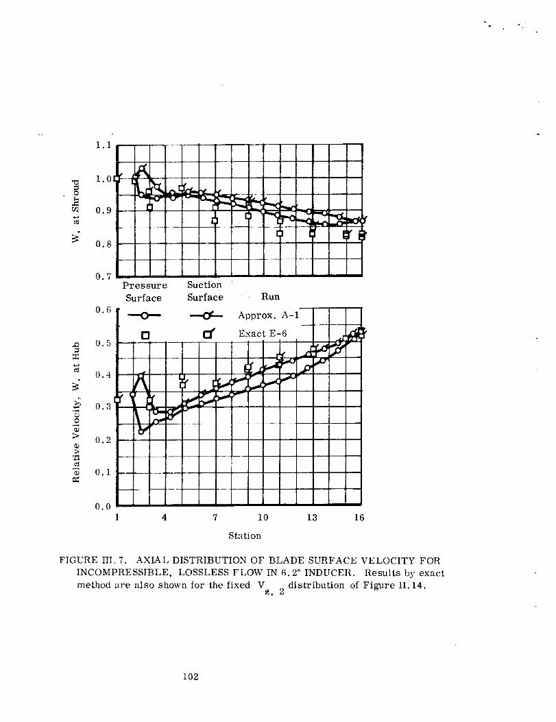
a
1.1
0.8
0.7Pressure Suction
Surface Surface
0.6--o-- --o e--
0.5 - _
Run
Approx. A-1
Exact E-6
0!0.2
_D
0.1 .... ..
0.0
1 4 7 10 13 16
Station
FIGURE III. 7. AXIAL DISTRIBUTION OF BLADE SURFACE VELOCITY FOR
INCOMPRESSIBLE, LOSSLESS FLOW IN 6.2 ° INDUCER. Results by exact
method are also shown for the fixed V distribution of Figure II. 14._, 2
102

_D
:{
4-a
.16
.12
.O8
•O4
0.00
-0 04
o
d
_9
_D
Pressure Suction
16 1 Surface Surface]
12 E] [_1 i I
O8
04
O0
-0 04
1 4 7 10 13 16
Station
FIGURE III.8. AXIAL DISTRIBUTIONS OF BLADE SURFACE PRESSURE
FOR INCOMPRESSIBLE, LOSSLESS FLOW IN 6.2 ° INDUCER. Results
by the exact method are also shown for the fixed V distributionof_, 2
Figure II.14.
103

1.1
1.0
0.9
0.8
0.7I I fl I
0.7
0.6
,m
0.5
0.4
_9O
0.3CD>CD
"-_ 0.2,.....¢
0.1
0.0J .....
1 4 7 10 13 16
Station
d
FIGURE III.9. AXIAL DISTRIBUTIONS OF BLADE SURFACE VELOCITY
FOR INCOMPRESSIBLE, LOSSLESS FLOW IN 12 ° INDUCER, SHOWING
CORRELATION WITH EXACT METHOD FREE PRESSURE RESULTS.
104

1.7
0.7
0.7Pressure Suction ' ' '
Surface Surface Run-lJ
0. 6---0"-- ---0 ¢'- Approx. A- 10 -- -_ . r[ _-
Oo 0 ,,,m
1 4 7 10 13 16
Station
FIGURE III. 10. AXIAL DISTRIBUTIONS OF BLADE SURFACE VELOCITY
FOR INCOMPRESSIBLE, LOSSLESS FLOW IN 12 ° INDUCER, SHOWINGCORRELATION WITH EXACT METttOD FORCED PRESSURE RESULTS.
105

g
084.a
04
, t:l (']O0 . r
-o.04 _,,o'
¢.)
.m,i
r_
-0
Pressure Suction
20 Surface Surface Run [ [J
---O--- _ Approx. A-10 ......... I_ i_ "_ rJ-
16 ___-[_. [_ Exact E-7 - I:A]_O_ D'I l'O'a'_ic _ i
I-1....... i '12
l,;y_ _ _,._r 'o8 _ ._" ,F E ,r
oo _._
O4
1 4 7 10 13 16
Station
FIGURE III. 11. AXIAL DISTRIBUTIONS OF BLADE SURFACE PRESSURE
FOR INCOMPRESSIBLE, LOSSLESS FLOW IN 12 ° INDUCER, SHOWINGCORRELATION WITH EXACT METHOD FREE PRESSURE RESULTS.
106

_Q
d
.20! I 7'
.16
.12
.08 Oj ' [
.04 II
.oo "_r" tf
-0.04 _
!
t
_j
i_r--
, ¢if:
i [
r ir
I
J
I
g,._"
[
I,[., • :f-_f
[ ; _r ,_:r
__ p_
!
!
.2O
.16,.Q
4_
¢_ .12
d.08
_JcD
.04
m 00
Pressure
Surface
Suction
Surface
--6--
i ! ! i
Run
Approx. A-10 "_
Exact E:8 I _.X_i_
,--o--
13i ! |
-- ------+------P---,-e-- [
-0.04 _ ' "1 4 7 10 13 16
Station
[
FIGURE III. 12. AXIAL DISTRIBUTIONS OF BLADE SURFACE PRESSURE,,FOR
INCOMPRESSIBLE LOSSLESS FLOW IN 12 ° INDUCER, SHOWING CORRELATION
WITH EXACT METHOD FORCED PRESSURE RESULTS.
107

O
[]
Zx
Run No. Method
A- 10 Approximate
E-8 Exact: Forced Pressure
E-7 Exact: Free Pressure
Relative
VelocityW
• 72
.7O
.68 r./
/
//
............ f
.66 _ [] Z
•64 4
.60 _
Static Pressure
P
.14
• 12 t
.10
.O8
.O6
. O4
A
z
0 0 0p s
Circumferential Position, 0
FIGURE III. 13. BLADE-TO-BLADE DISTRIBUTIONS OF PRESSURE AND
RELATIVE VELOCITY, SHOWING COMPARISON OF EXACT AND
APPROXIMATE METHODS. Incompressible lossless flow in 12 _
inducer at the central interior point, _ = .7600 and r - .7556.
108
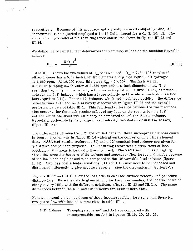
w •
respectively. Because of this accuracy and a greatly reduced computing time, all
approximate runs reported employed a 4 x 16 field, except for A-l, 3, 10, 12. The
approximate positions of the resulting three annuli are shown in figures HI. 23 and
III. 24.
We define the parameter that determines the variation in loss as the machine Reynolds
number:2
_rt,1Rm =" v (HI. 31)
Table III. 1 shows the two values of R m that we used. R m -- 2.5 x 10⁷ results ifeither inducer has a 5.37 inch inlet tip diameter and pumps liquid 36°R hydrogen
at 9,550 rpm. At 19,100 rpm, this givesR m= 5 x 10⁷ . Similarly we get
2.5 x 10⁷ pumping 267°F water at 9,550 rpm with a 6-inch diameter inlet. The
resulting Reynolds number effect, (cf. runs A-4 and A-5 in figure IH. 14), is notice-
able for the 6.2 ° inducer, which has a large solidity and therefore much skin friction
loss (equation I. 14). For the 12 ° inducer, which had much less solidity, the difference
between runs A-13 and A-14 is barely discernable in figure III. 15 and the overall
performance data of table HI. 1. This frictional difference between the two machines
also accounts for the much greater effect of any loss on the results for the 6.2 °
inducer which had about 70% efficiency as compared to 95% for the 12 ° inducer.
Especially noticeable is the change in exit velocity distributions caused by losses,
(figure III. 14).
The differences between the 6.2 ° and 12 ° inducers for these incompressible loss cases
is seen in another way in figure III, 16 which gives the corresponding blade element
data. NASA test results (reference 31) and a 12 ° constant-lead inducer are given for
qualitative comparison purposes. Our resulting theoretical distributions of loss
coefficient _ appear to be qualitatively correct. The NASA inducer has a high -_
at the tip, probably because of tip leakage and secondary flow losses and maybe because
of the low blade angle at outlet as compared to the 12 ° variable-lead inducer (figure
II. 18). Our loss coefficients (equations I. 14 and I. 15) may need to be increased and
distributed differently to give accurate results. (See the discussion in Section IV. )
Figures III. 17 and III. 18 show the loss effects onblade surface velocity and pressure
distributions. Here the data is given simply for the mean annulus, the location of which
changes very little with the different solutions, (figures III. 23 and III. 24). The samedifferences between the 6.2 ° and !2 ° inducers are evident here also.
Next we present the comparisons of these incompressible, loss runs with those for
two-phase flow with loss as summarized in table IH. 1.
6.2 ° Inducer: Two-phase runs A-7 and A-9 are compared with
incompressible run A-5 in figures III. 19, 20, 21, 23.
109

• 21
• 2O
¢q
_-.19>
.18o
>,I7
._.-i
_ .16
.15
.14
_:.o5>
.04
2.03
02
Run Field
.07 [_ A-1 8x16
A-2 4x16
.06 -- - A-3 8x16A-4 4x16
V A-5 4x16
.01
0
a m
oo (No Loss)
co (No Loss)5x10 7
5x10 7
2.5x10 7
_L
>
oO
0)>
,F-t
<
.17
¢q
.16
.15
.14
.13
2 r't"
08 -5_
•- 07
.O6
• 12 .05.7 .8 .9 1.0 .7 .8 .9 1.0
Radius. r
FIGURE III. 14. EFFECT OF LOSSES ON RADIAL DISTRIBUTIONS OF OUTLET
VELOCITY AND PRESSURE FOR INCOMPRESSIBLE FLOW IN 6.2 ° INDUCER,
Note accuracy of results of runs with three annuli (4x16) as compared to those
for seven annuli (8x16). Also note Reynolds Number effect in runs with loss.110
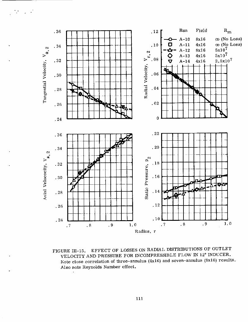
.36 .12
¢,q
>
oO
• 34
.32
.10
.O8
¢.q
>
O6o 30 _ •
_ _ .04
_. 02
• 24 0
Run Field
---O--- A-10 8x16D A-11 4x16
---_-- A-12 8x16
A-13 4x16
A-14 4x16
a m
(No Loss)
co (No Loss)5x10⁷
5x10⁷
2.5x10⁷
c,
d>
oooo
o
M<
.32
.3O
.28
.26
.24
-- .12
.10
.7 .8 .9 1.0 .7 .8 .9 1.0
Radius, r
FIGURE III-15. EFFECT OF LOSSES ON RADIAL DISTRIBUTIONS OF OUTLET
VELOCITY AND PRESSURE FOR INCOMPRESSIBLE FLOW IN 12 ° INDUCER.
Note close correlation of three-annulus (4x16) and seven-annulus (8x16) results.
Also note Reynolds Number effect.
111

¢Y
--O-
--o--
¢9
O
Run Rm
A-3 5 x 10⁷
A-4 5 x 10⁷
A-5 2.5 x 10⁷
A-12 5 x 10⁷
A-13 5 x 10⁷
A-14 2.5 x 10⁷
NA SA
Ref• 31
p.44
4 x 10⁶
Field
8x16
4x16
Inducer
6.2 °
6.2 °
4 x 16 6.2 °
8 x 16 12 °
12 °4x16
4x16
Test Data
12 °
NASA 12°
Notes
See Table III. 1 for
further information on
these analytical results.
0 = .1570 a = 1.9
Cold Water: v _ 1 csConst.Lead
1. O0
• 9O
• 8O
.70
• 60
• 5O
• 4O
f Hub of Ref.
NASA Inducer
AO
6p _.dw
j.O
,.--¢ b_ _ q
F Hub for allother data
• _'f_
I-4
I
L
]3
©
L)
2
• 2O
.10
0.5 0.6 0.7 0.8 0.9 1.0
I
gP
Is"
r-r- i I
Radius, r
FIGURE III. 16. COMPARISON OF INCOMPRESSIBLE FLOWS WITH LOSS FOR
6.2 AND 12 ° INDUCERS. RADIAL DISTRIBUTIONS OF OUTLET ANNULUS
EFFICIENCY AND LOSS COEFFICIENT. Also shown are experimental results
for a fiat plate 12 ° NASA inducer with a constant hub-to-tip radius ratio•
112

w v
Run
No.
O
A-2
[]A-5
BladeSurface Description
Pressure
Suction
Pressure
Suction
No Loss
Loss
R m = 2.5 x i0?
0.8
oov--4
_0.7
¢9
0.6
0.2
_0.1
4
.... _ 0 0 _i_,,,0-_. 0 ,,.,, C3]
o ,.,_._..8''=" _.__,_----_ X_Cr _-_•O.._.- m*
7 10 13 16
Station
FIGURE HI. 17. COMPARISON OF BLADE SURFACE DATA FOR
INCOMPRESSIBLE FLOWS WITH AND WITHOUT LOSS FOR 6.2 °
INDUCER. Axial distributions of velocity and presure in mean
annulus.
113

RunNo,
OA-11
[]A-14
BladeSurface
Pressure
Suction
Pressure
Suction
Description
No Loss
Loss
R =2.5x10 7m
o
>
>°r,,l
o
0.8
0.7
0.6
T
4
¢D
tD
CD
¢9
+0.2
+0.1
0jE __
-0.1 .-
1 4 7 I0 13 16
Station
FIGURE III. 18. COMPARISON OF BLADE SURFACE DATA FOR
INCOMPRESSIBLE FLOWS WITH AND WITHOUT LOSS FOR 12 °
INDUCER. Distributions of velocity and pressure in mean annulus.
114

12°Inducer: Two phaseruns A-16 and A-18 are compared withincompressible run A-14 in figures III. 19, 20, 22, 24.
These six runs were all made at the same machineReynolds number, Rm = 2.5 x 10⁷.Single-phase liquid flow existed just upstream of the blading andthe inlet flow co-efficients 01, f for the 6.2° and12° inducers were 0. 083 and 0. 1763respectively.
In order to understandthe two-phase phenomenaas shownin these results, we shouldfirst review the performance parameters involved. For a given inducer, reference 8showedthat our flow model analyzes the influence of four dimensionless parameters ona fifth one. We express this as follows:
• = _(01,f, Rm, _sp, O ) (HI. 32)
where the following definitions apply:
Total head rise coefficient
T = goA_ (HI. 33)
Ut, 12
Inlet liquid flow coefficient
WT01, f - (HI. 34)
of A 1 Ut ' 1
Machine Reynolds number
2rt,1
R m -V
Cavitation coefficient
(III.31)
_i - Psatk_sp = (III 35)
P_[_ 12go Ut'
Vaporization parameter
B 12 Of T*® - -- Ut, - Ut, 12 (III. 36)go go
115

where T* is defined in equation (I. 8). Table III. i lists these for each run. Becauseof the many existing cavitation parameters, we have listed other useful forms intable III. 1 besides 't'sp. These all express dimensionlessly the excess of inlet pressureover vapor pressure."
Suction specific speed:
S -= (III. 37)
Cavitation number:
k _:
Pl - Psat
Pf Ut, 12
2go(1 + _1, f2)
(m. 3s)
The effect of different combinations of inducer speeds and fluids at constant values
of these cavitation parameters is expressed by the vaporization parameter 0,
(equation III. 36). Accordingly, we made two-phase runs for various combinations of
•I,_ and @, holding Rm and 01, f constant. Figures III. 19 through III. 24 give data for
9 _ 10 and 1000. * Even though we used a lower 'I'sp for the 9 = 10 case, the volumeof vaporizing fluid, and its effect on performance was considerbly less than for the
9 = 1000 cases. Therefore, the incompressible case and the 9 = 1000 case for each
inducer are presented in figures III. 19 and III. 20. The exit radial distributions,
given in the first of these figures, show the effects of internal two-phase motion
primarily on the pressure. This is shown also in the overall performance data of
table III. 1. The loss coefficient data in figure III. 20 shows that most of the effects
are felt at the tip, as would be expected. The fact that we did not get more two-phase
performance deterioration (as compared to non-cavitating values) is probably due to
our omission of tip leakage vortex vaporization effects and our apparently low loss
factors, which apparently did not allow for the actual distribution of secondary flow
losses; (see foregoing discussion of incompressible flow with loss). Also, if we had
concentrated an additional annulus near the shroud, our results might have shown
more performance deterioration. The average relative velocity of this annulus would
be higher and would therefore lead to larger local pressure drops and the consequent
vapor formation. In early check-out work that we did on this method using a 2 x 16
field (one annulus only) we were able to obtain two-phase solutions at slightly lower
NPSH than was possible with the 4 x 16 field.
* For dimensional examples to which these solutions apply. See Table IV. 1.
116

O
--O-
Run No. O Flow Inducer
A-5 6"20Incompressible
Two-PhaseA-9 1000 6.2 °
A- 14 Incompressible 12"
A-18 1000 Two-Phase 12 °
.28
.26 _,_
.__ .22 ...... ./o
.20
p
.16
.14 .....
> .08
"_ . 06 •
__
02 _ _. __--
.01
36
34
cq
>_ 32
"_ 30
"6>
1
18'N
<
16
L@-"
-i
! -
I
4
"1.
.18
.16
12$..,
fl .lOr_
.O8
.O6.14
.7 .8 .9 1.0 .7 .9 1.0.8
Radius, r
FIGURE HI. 19. EFFECT OF TWO-PHASE FLOW WITHIN BLADES ON RADIAL
DISTRIBUTIONS OF" OUTLET VELOCITY AND PRESSURE FOR 6.2 AND 12 °
INDUCERS (R m = 2.5 x 10⁷).
117

• I
---O-
--z2--
----0 Do
Run
No. Description Inducer
A-5 Incompressible 6.2 °
A-9 Two Phase 6.2 °
A-14 Incompressible 12 ¢
A-18 Two Phase 12 °
_9
O
1.00
0.90
0.80
0.70
0.60
0.50
. = a
V"V_
%%
0,20
-P-I
°r,,_
orj
if]O
0.10
0.00
Radius, r
FIGURE III. 20. COMPARISON OF OUTLET PARAMETERS FOR TWO
PHASE AND INCOMPRESSIBLE FLOWS WITH LOSS IN 6.2 ° AND 12 °
INDUCERS. Reynolds number, R m = 2.5 x 10⁷. Radial distributions
of outlet annulus efficiency and loss coefficient at blade trailing edge.
118
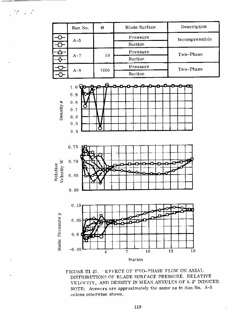
--O-
--D-
--_--
--O-
O.
¢9
Run No.
A-5
A-7
A-9
1.0_
0.9
0.8
0.7
0.6
0.5
0.4
0
10
1000
kl
Blade Surface Description
Pressure
Suction
Pressure
Suction
Pressure
Suction
Incompressible
Two-Phase
Two-Phase
=
I !i
[ . Ii
I
i
0.75 I _ _ _ ,
O. 60 '
0.10
0.05
0.01
_,_ -0.05
rV
.2wD- x:_
pO- ,O.,_
I0 13 16
Station
FIGURE II1.21. EFFECT OF T_rO-PHASE FLOW ON AXIAL
DISTRIBUTIONS OF BLADE SURFACE PRESSURE, RELATIVE
VELOCITY, AND DENSITY IN MEAN ANNULUS OF 6.2 ° INDUCER.
NOTE: Answers are approximately the same as in Run No. A-5
unless otherwise shown.
119
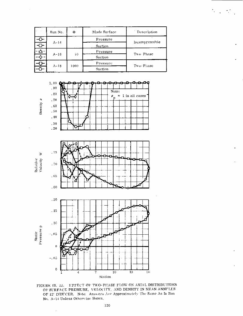
-O-
--[:3-
_-6--:_--O-
--O--
Run No.
A-14
A-16
A-18
i
O
10
tO00
Blade Surface Description
Pressure
Suction
Pressure
Suction
Pressure
Suction
Incompressible
Two-Phase
Two-Phase
o_
e,
1.00
.90
.80
.70
• 60
.50
• 40
.30
.20
pp = 1 in all cases
_2 .;0 i i / ' i
.60
ea
t.
.2O
.15
.10
_.05
-.05
-t.....LI ::: : ::.....i......i 4 " 10 13 16
Station
FIGURE III. 22. EFFECT OF TWO-PUASE FLOW ON AXIAL DISTRIBUTIONS
OF SURFACE PRESSURE, \:ELOCII'Y, AND DENSITY IN MEAN ANNULUS
OF 12" INDUCER. Note: Answers Aro Approximately Tile Same As Ial Run
No. A-14 Unless Otherwise Shown.
120

Tip
Hub
1.0
0.8
= 0.6
0.4
0. 333
0.2
m'[5".:':..':i
Tip Annulus'
; Axis of Rotation
(a) Extent of Two Phase Flow
Region
of Two Run
Phase No.
Flow*
Key
None A-14
Type
of
Flow
Incompressible
Mild Cavitation
Severe Cavitation
A-16
i
A-18
-431--
--_-.
*All portions of inducer contain liquid
flow unless otherwise indicated.
c_
d
y]
¢9
b_
co><
0.2
0.I
(b) Average Pressure in Mean Annulus
1
4 7 10 13 16
Station
FIGURE III. 23. DOMAINS OF TWO-PHASE & INCOMPRESSIBI,E FLOWS
FOR 6.2 _ INDUCER. Losses included: R m = 2.5 x 10⁷ . Postions
of streamlines are approximately as shown for all 3-annulus runs
with this inducer, Note that extent of two-phase region increases
with severity of cavitation (part a), and that pressure buildup is
correspondingly delayed (part b).
121
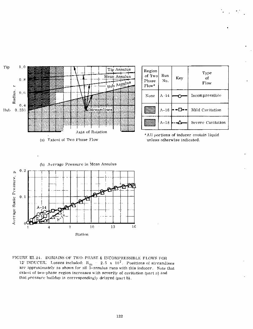
1.0
0.8
O.(;¢_
0,4
0,333
(a)
:-t";;%-%".
Extent of Two Phase Flow
Region Typeof Two Run
Key ofPhase No.
FlowFlow* -,
None A-14 @[ Incompressible
FA
*All portions of inducer contain liquid
unless otherwise indicated.
A-16 --0-- Mild Cavitation
A-18 ,,,,,_--- Severe Cavitation
(b) Average Pressure in Mean Annulus
0.2
_rl ---.
0.1
A-14
< 0(1 4
.................. 1__[__
........T..... 1--}2_,_, _
7
°7L10 13 16
Station
FIGURE III. 24. DOMAINS OF TWO-PtIASE & INCOMPRESSIBLE FLOWS FOIl
12 _ INDUCEFC Losses included: R m 2.5 x 10⁷ . Positions of streamlines
are approximately as shown for all 3-annulus runs with this inducer. Note that
extent of hvo-phase region increases with severity of cavitation (part a) and
that pressure buildup is correspondingiy delayed (part b).
122

The fact that the upstream regions within inducer blading unload at low @sp and high O
is shown in figures III. 21 and III. 22, where the distributions of blade surface density,
velocity and pressure in the mean annulus are given in three cases for each inducer.
First, the incompressible case gives the "front loading" characteristic of inducers.
Second, the O = 10 case produces some front unloading and a density reduction on the
suction side of the blade. Finally the O = 1000 case produces more unloading and a
greater suction side dens!ty reduction. Thus it appears that even though _I'sp = 0in the cases of ® = 10, there was only mild _cavitation due to the low vapor volume.
O = 1000 at higher _sp was the more severe case as evidenced by the overall perfor-mance deterioration that occurred, (see figures IV.4 and IV. 3) In all cases the
essentially unchanged outlet velocities require that the blades must carry the same
load. It merely shifts back farther into the inducer under cavitating conditions.
A more graphic illustration of these same two-phase effects appears in figures III. 23
and III. 24, where the portions of the machine occupied by two-phase fluid are shown
in part (a). Table III. 1 shows that we probably did not compute runs A-7 and A-9
for the 6.2 ° inducer with sufficient streamline balancing accuracy as compared with
run A-18 for the 12 ° inducer on this basis. This accounts for the lack of vapor in
at least the mean annulus between stations 2 and 3 (j' = 3) in figure III. 23. The
unloading phenomenon is illustrated in parts (b) of these figures in the effect that it
had on the distribution of average static pressure rise in each case.
C. CONCLUDING REMARKS ABOUT THE APPROXIMATE METHOD OF SOLUTION
The streamline balancing method of obtaining a rapid, approximate solution to single
and two-phase inducer flows gives accurate numerical results even when only three
annuli (four streamlines) are used for the calculations. It is a way of quickly judging
or grading an inducer to determine whether the more detailed and lengthy analysis by
the exact method is merited. (An exact description of the flow can be obtained only by
this latter method, and by using a sufficiently fine grid. )
In this approach we employed assumptions that appear to be justified for typical inducers,
but which may cause some inaccuracies. These are the omission of the meridional
streamline curvature and blade force effects and of the upstream and downstream flow
regions; the restriction of flow to concentric annuli; and the blade-to-blade analysis
assumptions (Section III. A. 4). Results for incompressible flow are in accordance with
known data where the same assumptions are used, (e. g., reference 6).
Results for two-phase flow are qualitatively correct; and they demonstrate the ability
of the method to describe the blade loading shifts that occur at low NPSH. The loss
factors appear to be weak, because these two-phase effects did not cause sufficient
pressure rise deterioration as compared to that of tests. For example, the comparison
of our 12 ° variable-lead inducer with the NASA 12 ° constant lead one in Figure III. 16
shows greater loss at the blade tips of the latter, which yielded lower efficiency than
we obtained on our somewhat similar configuration. However, empirical adjustment
of these factors could be used to offset any inadequacies, since the loss mechanisms
123
appear to give qualitatively goodresults. (It might also be necessary to concentrateone of the annuli near the shroud to produce two-phase performance deterioration. )In the following section, we discuss this possibility of loss factor adjustment as weuse these results in the analysis of performance and design requirements.
The Fortran IV listings for this method currently include a blade coordinate subroutinefor radial-element, variable-lead blades. These listings together with othercomputational details including running time estimates appear in Appendix D.
124
i
SECTION IV
INFLUENCE OF FLUID PHENOMENA ON THE
PERFORMANCE AND DESIGN OF INDUCERS
In the foregoing sections we presented solutions of inducer flows using analytical
methods. These included a model for real fluid effects that can be changed in
accordance with experimental evidence without too much difficulty. In this section
we review the results of those and other solutions that include these effects to
determine the capabilities of our model for predicting performance and optimizing
designs. Since an inducer generally experiences some two-phase flow and losses,we will first examine specific properties of our relations (I. 7) and (I. 13) for
describing these phenomena, (Section IV. A). Then in Section IV. B, we will
summarize our predictions of overall performance and their correlations with
recent theories for scale or fluid thermal effects. This is followed by resulting
observations about design optimization, (Section IV. C).
A. CHARACTERISTICS'OF EQUILIBi_I_ T_WO-PHASE FI_OW
AND LOSS MODE L _ ;
lo Two Phase Flow at Inducer Inlet
A homogeneOus two-phase or single-phas e flow in thermodynamic
equilibrium is implied by equations (I. 7)and (I. 13). Combined with
various forms of the momentum and continuity laws, these relations
enable us to analyze situations from three-dimensional inducer motion
to one-dimensional duct flow (reference 8, p. 4-54).
Of particular interest is the fluid state for vaporizing flow at the inducerinlet. This information is required for the boundary conditions of the
analytical methods of solution, (Section II and III). Also, if such an
upstream two-phase condition does exist, we need this to determine
the proper design blade angles at inlet. In fact, Adams (reference 32)
uses equilibrium vaporization theory to explain his test results of
lifting boiling fluid in a pump inlet line.
Accordingly, equation (I. 7) and (I. ! 3) are used with continuity and the
streamline momentum equation for a one-dimensional analysis of the
upstream duet flow. The latter equation in the absolute frame'is
(cf. equation I. 12) "
go dp- VdV + F
A special case is the essentially lossless acceleration that occurs in
a machine having a converging inlet duct. Here, the density is
(IV. 1)
125

expressed in terms of the velocity as follows:
P= Pf_
1
B
_-o (V 2 - Vsat 2) + 1
(IV. 2)
or in terms of the corresponding dimensionless parameters for inducers,
Pf = = " A
0 (012 Vsat 2)+1
(IV. 3)
where Vsa t is the velocity at the saturated liquid condition. Note that Vsa t
is zero if the inducer is sucking boiling liquid from a tank. We used this
equation to calculate the two-phase inlet densities and pressure for our
zero-NPSH runs A-6 and A-15 (table III. 1).
Corresponding to(oP----_are the volume ratio of vapor-to-liquid for the
mixture (_y_V)and thel"ratio of the two-phase inlet flow coefficient to that
which wou_d exist for liquid at the same mass flow rate 01/(31, f,(equation I. 7):
and
-1 = 2"* (Psat - P) (IV. 4)
V 1 0 1 1
V1, f 01,f ( P/Pf)I(w. 5)
Aside from considerations of whether a given inducer can pump fluid with
a high inlet (V/L); we see from equation IV. 5 that when it pumps liquid at
inlet, i.e., (V/L)I -- 0, an excessive incidence angle between liquid and
blade would result with a machine designed to handle the same mass flow
rate at such high (V/L)I. To illustrate this fact, figure IV. 1 shows plots
of the preceding three equations for various values of the vaporization
parameter O defined by equation (IH. 36).
In all this work we must remember that the barotropic state relation (I. 7)
for two-phase motion is good only for low mixture quality x, where
126
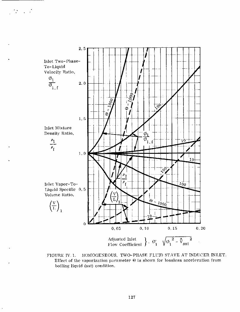
Inlet Two-Phase-
To- Liquid
Velocity Ratio,
01
Inlet Mixture
Density Ratio,
Pl
Pf
Inlet Vapor-To-
Liquid Specific
Volume Ratio.
!2._ I t
2.0 i _ /
_ ,j -- _
i_oo11
/ __,." __A_. ,--- "7"I- 10
0.05 0.10 0.15 0.20
Adjusted Inlet } , t012 ^ 2Flow Coefficient " 01 - Vsat
FIGURE IV. 1. HOMOGENEOUS, TWO-PHASE FLUID STATE AT INDUCER INLET.
Effect of the vaporization parameter O is shown for lossless acceleration from
boiling liquid (sat) condition.
127

X _
T_ O .( dsf 1 -)(Psat- P) (Psat- P) - pf Pv
\-_p " Sfg \_g- ]sat (pg-1) satAA
6)
and the dimensionless suppression pressure is
A goAPv - _ (Psat-P)
Pf(IV. 7)
We note further that the dimensionless form of the state equation (I. 7) is
A p 1
P-- _ ---- AI+OAp v
(IV. 8)
For most cases involving this kind of flow, x is small for the minimum valuesof 9 encountered, and this relation is an adequate representation of the
equilibrium model. For example, in liquid hydrogen at 36°F, (reference 19)
B _ (pf T*._ = sec 2go \----_] .0002 ft 2
Pf/Pg = 52.8
A
By selecting the values in equation IV. 8 that give minimum p, (and therefore
maximum x), we have
O (= B 12-- Ut, )=40go
A
APv =.1
We obtain from equations (IV. 4,6, 8), using Pf / Pg from reference 19
x = . 077
P/P f = .2
V/L (= O A_v) = 4
For most fluids, T* is roughly proportional to Pf/Pg; so, we conclude from
equation IV. 6 that this value of x is typical of that obtained for the largest
128

A
concentrations of vapor in inducers. Since A Pv is quite large, (comparedwith the inducer head-rise coefficient @ -- similarly defined in equation
III. 33), and since this example is for a high inducer inlet tip speed, viz.,
Ut, 1 = 447 ft/sec., our barotropic relation (I. 7) or (IV. 8) should beapplicable in most cases. (Refer to the barotropicity dicussion in
Section I. A. 1).
2. Discussion of Losses
A good prediction of equilibrium two-phase and liquid flow within an
inducer depends on the accuracy of the factors and methods for evalu-
ating losses, as well as the equation of state. Besides blade tip leakage,
two types of loss can be distinguished, (equation I. 13); viz., skin friction
or Reynolds-number-dependent losses, and diffusion or inertial losses.
For friction losses we are using an empirical relation (equation I. 14)
for smooth pipes to express the friction factor f. This loss also depends
on the local hydraulic diameter of the channel which is assumed constant
for all annuli at a given station. A correction to this is probably necessary
to account for the additional skin friction arising from the secondary flow
caused by blade-to-blade pressure differences. But secondary flow losses
might be conveniently described by an appropriate adjustment of thediffusion loss factor.
A good diffusion description is especially important for inducers with two-
phase flow, since the sudden disappearance of vapor that can occur
probably results in a dumping of at least part of the accompanying change
in relative velocity head (references 32 and 33). This sudden diffusion
head loss, (see equation I. 13), from station j to j + 1 in the inducer may
be given by
HL, d _.tWj2 - Wj + 12 /= - -- (IV-9)2go
where Wj+I<W j. In our model we expressed _"as a function of the ratio
Wj+I/Wj (equation I. 15), making it possible for us to describe only adiscontinuous change of W. If the factor _'is to include separation losses
that occur over some finite distance, we would need to modify this
function (equation I. 15) in one or more of the following ways: (a) limit the
number stations j; (b) increase the strength of _; (c) make _ a constant that
is independent of W; or (d) make _*dependent on the diffusion factor D. A
measure of the overall blade loading, (see definition on page 153 of
reference 33), the distribution of D would first need to be estimated from
a preliminary solution or one-dimensional analysis of the machine.
As a result of our inducer solutions with loss, it appears that some combi-
nation of (a), (b) and (c) would give better answers and could be easily
129
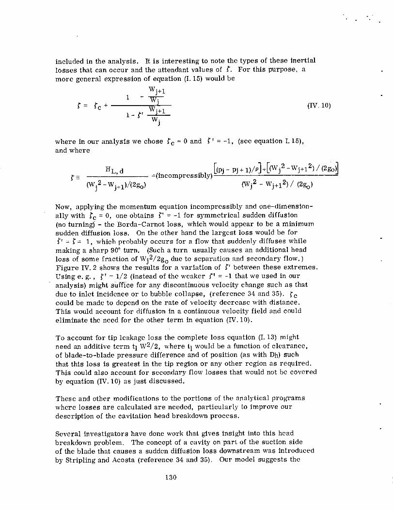
included in the analysis.losses that canoccur andthe attendant values of _'.more general expression of equation (I. 15)would be
Wj+I1
_= _c +1-/" wj+I
wj
It is interesting to note the types of these inertialFor this purpose, a
(IV. I0)
where in our analysis we chose _'c = 0 and _" = -1, (see equation I. 15),
and where
=(incompres sibly)
(Wj 2 -Wj+l)/(2go) (Wj2 - Wj+12 )/ (2go)
Now, applying the momentum equation incompressibly and one-dimension-
ally with _'c = 0, one obtains _" = -1 for symmetrical sudden diffusion
(no turning) - the Borda-Carnot loss, which would appear to be a minimum
sudden diffusion loss. On the other hand the largest loss would be for
_' = _= 1, which probably occurs for a flow that suddenly diffuses while
making a sharp 90 ° turn. (Such a turn usually causes an additional head
loss of some fraction of Wj2/2g o due to separation and secondary flow. )Figure IV. 2 shows the results for a variation of _" between these extremes.
Using e. g., _" -- 1/2 (instead of the weaker _' = -1 that we used in our
analysis) might suffice for any discontinuous velocity change such as that
due to inlet incidence or to bubble collapse, (reference 34 and 35). _c
could be made to depend on the rate of velocity decrease with distance.
This would account for diffusion in a continuous velocity field and could
eliminate the need for the other term in equation (IV. 10).
To account for tip leakage loss the complete loss equation (I. 13) might
need an additive term t 1 W2/2, where t 1 would be a function of clearance,
of blade-to-blade pressure difference and of position (as with Dh) such
that this loss is greatest in the tip region or any other region as required.
This could also account for secondary flow losses that would not be covered
by equation (IV. 10) as just discussed.
These and other modifications to the portions of the analytical programs
where losses are calculated are needed, particularly to improve our
description of the cavitation head breakdown process.
Several investigators have done work that gives insight into this head
breakdown problem. The concept of a cavity on part of the suction sideof the blade that causes a sudden diffusion loss downstream was introduced
by Stripling and Acosta (reference 34 and 35). Our model suggests the
130

DiffusionI.xis s
Factor
(_c 0)
W.
J
Configuration (a)
1.o _ r =q-_
00 .2 .4 ,6 .8 1.0
Ratio of Downstreamto Upstream Relative I Wj+I
Velocities ] W.] Pj ]_
I _i_ wi 'i |j*
(pj - Pj_l ) =
(pj - Pj+l ) : 0
I°Wj. 1
go
lJ+lI
,'--. wj<IIII
(wj ._-i - wj)
Configuration (a)
Diffusion in Sharp. 90 ° Turn
Configuration (b)
Symmetrical Sudden Diffusion
IBorda-Carnot Loss)
FIGURE IV. 2. SUDDEN DIFFUSION LOSS FACTOR, _'. For discontinuous relative
velocity changes. Also applicable to continuous changes where appropriate spacing
of stations j in a finite difference calculation scheme is employed.
(See Equations IV. 9 and IV. 10).
131

presence of sucha cavity by yielding a low density in that region (seefigures Ill. 21 and 22). The shock theory of Jakobsen (reference 36)combined the cavity analysis with thermal concepts and could be used toadvantagein improving the loss descriptions in our three-dimensionalprograms. Two-phase sonic velocities (reference 37) can be very low,and the attendant mass-flow limiting process shouldoccur, (reference 38and reference 8, p. 4-55). Our model does produce choking if a solutionat too low a NPSHis attempted, and this is discussed in the followingsection.
B. PERFORMANCE AND SCALE EFFECTS WITH TWO-PHASE FLOW
1. Low-NPSH Tests of Inducers by the Analytical Program
We made a series of solutions with the approximate analysis program,
which includes unmodified loss relations (equations I. 13, 14, 15) to
determine the net positive suction head requirements of the two sample
inducers, (figures II. 12 and II. 18). All these analytical runs were made
at the same values of flow coefficient 01, stated in table IH. 1 for the
respective inducers. However two runs, A-6 and A-15, had negative
values of cavitation number k at inlet and therefore had two-phase flow
upstream of the blading. The liquid flow coefficient 01, f was therefore
lower than 01 for these two cases only (see footnotes to table III. 1),
both of which used O = 10. For the other data, we conducted three series
of runs at ® = 10, 40, and 1000 respectively on each inducer. In each
series we started at high NPSH, where the dimensionless form ,I_s is
given by
q., go (NPSH) 012
s - Ut, 12 ( _I'sp > 0)- _I,sp +
2 '(IV. 11)
and we lowered _sp until no solution could be obtained (choked flow), or
until q'sp = 0, (table Ill. 1). Table III. 1 lists only those two-phase
solutions that were obtained for the lowest possible _sp.
Figures IV. 3 and IV. 4 show the kind of pressure-rise-deterioration curves
that we obtained, starting with the value of _sp required to preventcavitation entirely and ending with the value for which no solution was
obtainable w except in the case of ® = 10, where solutions for q'sp = 0
did exist. For comparison, actual cold water (® _ 1,000,000) test
results of a NASA 12 ° constant-lead inducer are also shown in figure IV. 4,
(reference 31, p.47). Even though this reference inducer is somewhat
different from our 12 ° machine, the results indicate that our analytical
model reasonably predicts the choked-flow or zero-performance condition.
However, our curves have sharp breaks and therefore do not yield the
132
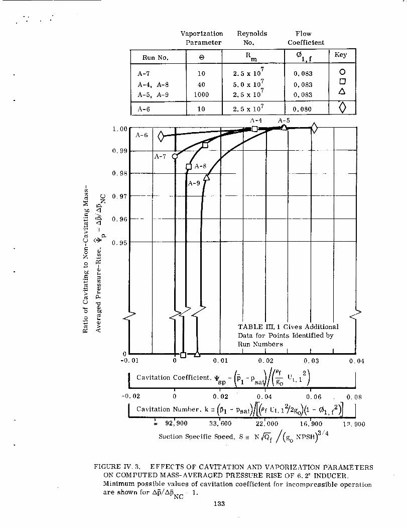
1.00
0.99
0.98
I
c) 0.97}5
>
c) <_ 0 95I
dOZ
@
O
Vaporization
Parameter
Reynolds
No.
Flow
Coefficient
Run No.
A-7
A-4, A-8
A-5, A-9
O
10
40
1000
Rm
2.5 x 10⁷
5.0x 10⁷
2.5 x 10⁷
_1, f
0. 083
0. 083
0. 083
A-6 I0 2.5 x 10⁷ 0.080
A-4 A-5
Key
0[3A
x/
. 3z
r_
-0.01 0 0,01
I Cavitation Coefficient. _I,sp-!
-0.02 ; 0.02
<
TABLE III, 1 Cives Additional
Data for Points Identified by
Run NumbersI I I I I
0.02 0.03 0.04
@1- Psal/(_--_fo Ut' 12)• lI I
0.04 0.06 0.08
1 ! I 192,900 33,600 22 000 16,900 1_,900
uctio oeed.
I Cavitation Number, ke@l-Psat)/[/P f Ut, 12/2go)0Igo
FIGURE IV. 3. EFFECTS OF CAVITATION AND VAPORIZATION PARAMETERS
ON COMPUTED MASS-AVERAGED PRESSURE RISE OF 6.2 ° INDUCER.
Minimum possible values of cavitation coefficient for incompressible operation
are shown for A_/A_N C : 1.
133

tm iii
cJ
i
oZ =
_o0
m
0)
o!
o m.-t Ot_
m N
1. O0
0.99
0.98
0.97
0.96
0.95
Run No.
A-14, A-16
A-17
A-I3, A-18
A-15
NASA Tests
(Ref. 31)
Vaporization
Parameter
-- t
-- .-a
T !i-0.02 0.01 0
Reynolds
No.
Flow
Coefficient
O
10
4O
1000
I0
1,000,000
Rm
2.5 x 10⁷
5.0 x 10⁷
2o5X 107
2.5x10⁷
4.0 x 10⁶
01, f
0.1763
0.1763
0.1763
0.1540
0.14
KEY
O
O
0
<>-_ A-13J
g )_ " I
A-I_A-15 ,_
IA-16()" / _,_-_o IA-171 ]
III!
!.... i
III$ .>
> > _-_: --- - <:_
I" '_ " -- TABLE Ill I gives additional
I [ data for points identified byI II i run numbers.
i. A i I I0.01 0.02 0.03 0.04 V 0.'12 0.13 0'.14
1 I _/(-Pi-Psat)/@(g°Ut'12) ICa_,itation Coefficient, _sp =- ^
-0.02 0_01 0 0.'02 0.'04 0.'06 0'¢)_ 0.'24 0.'26
I ...... I Cavitati°nC°efiicient' k--(Pl.-/_ Psa)/_(PfUt'l')/\l +012)12go ', ' f
' 43,300 30,'400 23'600, 19,900 16,800 '_/ 8.'600 7. 800
Suction Specific Se___ee_dsLS_-- N Q_---f / (go NPSH)3/4(S given for 0 : 0. 173, but error
is small for other (_)
FIGURE l_'. 4. EFFECTS OF CAVITATION AND VAPORIZATION PARAMETERS
ON COMPUTED MASS-AVERAGED PRESSURE RISE OF 12 ° INDUCER.
Minimum possible values of cavitation coefficient for incompressible
operation are shown for Ap/APNc - 1
134

the gradual decay of pressure rise with decreasing @sp evidenced byactual tests. This means that modifications to the loss factors and the
annulus positioning as inlet, as discussed in the foregoing section, are
probably necessary to extend the two-phase regions farther into the
inducers and to describe more accurately the losses due to bubble collapse,
i.e. the sudden disappearance of these regions, as illustrated in figures
IN. 23 and III. 24.
Such adjustments could also serve as a substitute for any lack of baro-
tropicity. Specifically, in the discussion of Section I. A. 1 we spoke of
the rise of vapor pressure of the liquid due to losses. If such a rise
occurs before all vapor is condensed by the rising inducer pressure, the
domain and effects of the remaining vapor could be significantly increased.
A stronger friction loss factor than that of equation (I. 14) might artificially
reproduce this by retarding the rise of inducer pressure by the slight
amount of the simulated vapor pressure change.
Table IV. 1 shows dimensional examples to which these analytical per-
formance results apply. According to our equilibrium theory, then,
liquid hydrogen can be pumped at 224 ft. per sec. inlet blade tip speed
in typical inducers at zero cavitation number. Doubling the tip speed
makes ® -- 40; and, as equation (IV. 8) shows, this causes more vapor at
a given pressure drop coefficient in the blading, preventing a solution atk=0.
2. Theory of Fluid and Scale Effects
The complete inducer analysis that we employ to find the NPSH limits
actually contains the explicit relationship, however complicated, between
the independent dimensionless parameters, Rm, 'IJsp and ® that determine
the performance 4, (expressed by the functional equation III. 32). How-
ever, we should try to discern in these and other results a simpler, under-
lying theory for these fluid and scale effects; especially the influence of
•I_sp and ®. We might then be able to determine the important inducer
design factors.
Specifically we are interested in how to predict the NPSH requirements
for various fluids and sizes of a given geometry for a fixed flow coefficient
_1, f. Therefore, we require the minimum value of the NPSH parameter _sfor which stable inducer performance is possible or for which the head
coefficient ,I, is some reasonably high percentage of the noncavitating value
_NC, (i. e. the value of no _s and ® influence), If Reynolds number effects
are small compared to those of fluid vaporization, the functional equation
(IH. 32) reduces for these purposes to
(TNC) =C°nstant= ( @-_NC) REQ'D (_s, min, ®) (IV. 12)REQ'D
135

TABLE IV.I
DIMENSIONALEXAMPLES OF SAMPLE INDUCERS
For inducers having same geometry as in Figure If. 12 of II. 18
Dimensionles s
Parameters of
Solution
VaporizationParameter
O
Consistent Set of Dimensional Conditions
to Which Solution Applies
Machine Liquid
Reynolds and
Number Temp,
Rm
Inlet
Tip Rotative Blade Tip Speed
Dia. * S__Speed* at Inlet
Dr, 1 N Ut, 1(Inches) (rpm) (ft/sec, )
10
4O
1000
2.5 x 10⁷ Hydrogen 5.37 9,550 224
@ 36°R
5.0 x 10⁷ Hydrogen 5.37 19,100 447
@ 36°R
2.5 x 10⁷ Water 6.00 9,550 250
@ 267°F
*NOTE: The only parameter that is directly connected with the inlet diameter
D, t or the speed N is the machine Reynolds number. For the usual
rS_ge of sizes, R m appears to have a small effect; so, the important
limitation for equilibrium two-phase flow is not Dt, 1 or N, but theirproduct, the tip speed
= rt, 1 Dt, 1Ut, 1 _2 = _ N
which is connected with the cavitation and vaporization parameters;
(see Table III. 1).
136

|
or
_l' S, min = _lJs, rain (E))(iv. 13)
Because 01, f is fixed in this problem, we could substitute either kmi n
or Smax for @ s, rain, where dimensionless relations between them (seeequations III. 34, 35, 37, 38 and IV. 11} are
2 XI,spk =
i + 01,f 2
and
_0 A1N Q_ 1,f _ rt,1 2
S=- =
(goNPSH)3/4 2_-- (q's) 3/4
2When applied to axial inducer inlets where A 1 = 7rrt, 1general form for the suction specific speed becomes
(I- }12), this
(IV. 14)
(IV. 15)
s= j01,f (i- }12)
2 _ ( T s)3/4 (IV.16)
Thus we are looking for the following function, (equivalent to equation
IV. 13):
Smax = Smax (®)01,f
or, dimensionally:
(IV. 17)
NPSHmi n = NPSHmi n (B)Qf (IV. 18)
Investigators have found empirical correlations that tend to support the
validity of the equilibrium equation (IV. 18). Stahl and Stepanoff (reference
13 and 14) first proposed a remarkably simple theory for that relationship,
also presenting their results. The basis of this theory is that the breakdown
of head rise under cavitating conditions is caused by a performance average
vapor-to-liquid volume ratio (V/L)p. Salemann's observations (reference 17)lend more support to this idea; and so does the work of Spraker, who also
defines the thermodynamic constant (B = Pf T*) so that the relative vapori-
zation characteristics of various fluids can be easily identified. For
137

100.
10.
¢q
¢qo
= .1oL)
tq
> .01o,p-I
0
.001
,0001
.000010 100 200 300 400 500
Water Temperature, ° F
FIGURE IV. 5, FLUID THERMODYNAMIC VAPORIZATION CONSTANT FOR WATER.
THE EFFECT OF TEMPERATURE IS SHOWN. W_ter corresponds to some other
fluids in the values of this constant at the temperatures shown,
138
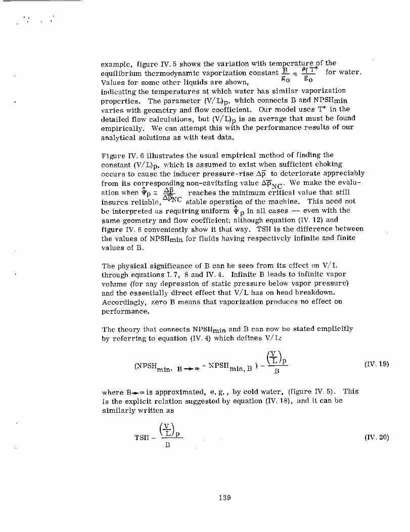
example, figure IV. 5 shows the variation with temperature of thePf T*equilibrium thermodynamic vaporization constant B =__ for water.
Values for some other liquids are shown, go go
indicating the temperatures at which water has similar vaporization
properties. The parameter (V/L)p, which connects B and NPSHmin
varies with geometry and flow coefficient. Our model uses T* in the
detailed flow calculations, but (V/L)p is an average that must be found
empirically. We can attempt this with the performance results of our
analytical solutions as with test data.
Figure IV. 6 illustrates the usual empirical method of finding the
constant (V/L)p, which is assumed to exist when sufficient chokingoccurs to cause the inducer pressure-rise A_ to deteriorate appreciably
from its corresponding non-cavitating value A_N C. We make the evalu-ation when _p =_ _ reaches the minimum critical value that stillinsures reliable, AP-NC stable operation of the machine. This need not
A
be interpreted as requiring uniform @ p in all cases -- even with the
same geometry and flow coefficient; although equation (IV. 12) and
figure IV. 6 conveniently show it that way. TSH is the difference between
the values of NPSHmin for fluids having respectively infinite and finitevalues of B.
The physical significance of B can be seen from its effect on V/L
through equations I. 7, 8 and IV. 4. Infinite B leads to infinite vapor
volume (for any depression of static pressure below vapor pressure)
and the essentially direct effect that V/L has on head breakdown.
Accordingly, zero B means that vaporization produces no effect on
performance.
The theory that connects NPSHmin and B can now be stated emplicitly
by referring to equation (IV. 4) which defines V/L:
(NPSHmin, B --_= - NPSHmin, B ) - B(IV. 19)
where B-_¢_ is approximated, e.g., by cold water, (figure IV. 5). This
is the explicit relation suggested by equation (IV. 18), and it can be
similarly written as
(-_)pTSH -
B(IV. 20)
139

1.0
Performance at B --_ 0
a_ .8¢D
¢D
"_ (-9 6
>
I
o ILlz
_ (% .4
°r.,._
.r-q
_" 20 "
0
0
IIII
tNPSH min, B
J_-- TSH B
Constant
Note: (V) = ConstantP
Might Yield Different ButI%
Satisfactory _p Values atVarious B.
Performance at B---- oo
NPSHmin, B _ oo
d_ ._------ 0 -------,._ +
Net Positive Suction Heat, NPSH
FIGURE IV. 6. NET POSITIVE SUCTION HEAD REQUIREMENTS FOR
INDUCERS. The influence of the thermodynamic vaporizationconstant B is shown.
140
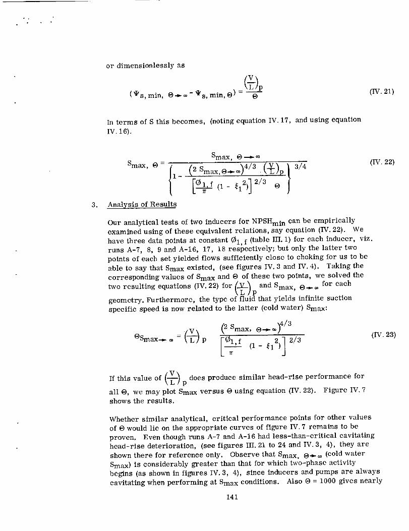
f
or dimensionlessly as
(_I's,min ' ®-_- @
(_-)p
s,min, O)= O(IV.21)
In terms of S this becomes, (noting equation IV. 17, and using equation
IV. 16).
.
Smax, O = ll -
l
Analysis of Results
Smax, 0 ""_ _
.(-})p/ 3/4
Our analyticaltests of two inducers for NPSHmi n can be empirically
examined using of these equivalent relations,say equation (IV.22). We
have three data points at constant 01, f (tableIII.I) for each inducer, viz.
runs A-7, 8, 9 and A-16, 17, 18 respectively; but only the lattertwo
points of each set yielded flows sufficientlyclose to choking for us to be
able to say that Smax existed, (see figures IV. 3 and IV.4). Taking the
corresponding values of Smax and @ of these two points, we solved the
two resulting equations (IV.22) for (L-_--)p and Smax, ®.,.¢_for each
geometry. Furthermore, the type of fluidthatyields infinitesuction
specific speed is now related to the latter (coldwater) Smax:
2 Smax, 0..._ _,) 4/3
,,
(IV. 22)
(IV. 23)
of (V_ does produce similar head-rise performance forIf this value\L! P
all @, we may plot Smax versus @ using equation (IV. 22). Figure IV. 7shows the results.
Whether similar analytical, critical performance points for other values
of O would lie on the appropriate curves of figure IV. 7 remains to be
proven. Even though runs A-7 and A-16 had less-than-critical cavitating
head-rise deterioration, (see figures IH. 21 to 24 and IV. 3, 4), they are
shown there for reference only. Observe that Smax ' @._ = (cold water
Smax) is considerably greater than that for which two-phase activity
begins (as shown in figures IV. 3, 4), since inducers and pumps are always
cavitating when performing at Smax conditions. Also ® = 1000 gives nearly
141

L
the same Sma x as at O -*-_. Finally, the 12 ° inducer has the greater
(V/L)p capability, which could be attributed to the larger amount of theinlet fluid relative incidence i not compensated by blade thickness. Note
that computations were made for faired blades, (figures II. 12, 18), whichin both inducers would have taken 0.64 ° of the incidence had full thickness
existed at inlet; i. e., all incidence in excess of this blockage amount then
causes leading edge blade loading and the attendant flow adjustments to the
internal two-phase activity.
A well-known experimental fact, the evident (V/L)p capability of this blade
fairing is illustrated by the two-phase no-loss run E-9 of the exact
analysis method (table II. 1). Here, the presently unadjusted upstream
stagnation stream surfaces are set at the relative flow angle (i = 0), and
the light load taken by them -- as they now act like faired blades -- nearly
eliminates two-phase activity within the blading itself, (figures H. 28 and
29). This "additional blading" enabled us to obtain that solution with a
lower NPSH (@ sp = 0 at O = 40)than was possible by the approximatemethod, which produced loading only on the actual blading.
To the extent that the preceding correlations and the experimental data
of references 13, 14, 17, 18 support the (V/L)p theory, as the connection
between S and O, we can propose a concluding theory about two-phase
activity within inducers. The observation that two-phase flow exists
at a much higher value of NPSH than the critical one suggests that two
fairly distinct flow regimes exist over the NPSH range:
a) For the range
NPSH incompressible > NPSH __ NPSHmin, ® --_flow
enough vapor forms to unload the inducer blades at inlet by an amount
compatible with the NPSH. This prevents the far greater volume of
vapor that would have choked the passage had the blade suction-side
pressure-drop not been reduced by the unloading (see figures III. 21 and
22). The extent of and density distribution of the vaporous region vary
with NPSH; but performance is affected only slightly, because the losses
associated with these redistributions of load near the leading edge are
small. Thus there are no O effects over this NPSH range, (figure IV. 7).
b) In the range
NPSHmin, O. _ 0o _ NPSH __> NPSHmin, 0
the passage is in the process of choking due to the formation of vapor
which is in excess of that required to satisfactorily unload the blades.
In contrast with regime (a), the flow in the leading portion of the inducer
142

is essentially one-dimensional. The additional V/L formation withdiminishing NPSH is more nearly uniform across the passageandis the only V/L Contribt_tingto (V/L)p. Thus the extent of this NPSHrange dependson ® (equationIV. 21); andWhen(V/L)u is reached, thepassageis sufficiently chokedto produce the critical'performance atNPSHmin. _ ._ -
Every geometry andflow-coefficient combination has the capability ofhandling a specific amount of this excess vapor (V/L). The results infigure IV. 7 suggestthat (V/L)p may be more or less directly dependenton the amount of available incidence in excess of that required forblade blockage. Thus if i = 3° or 4 ° total, a typical inducer might be
capable of (V/L)p = 0.5. The resulting plot of equation (IV. 22) using
Smax, ®._ _ = 2, (= 2 x_17,180 = 34,360 in "rpm-gpm-ft" units),is shown in figure IV. 7. A similar curve for typical centrifugal pumps
is also shown using Smax, ®._ = 1/2 (or 8,590). Higher incidenceprobably leads to more vapor due to excessive loading; therefore, no
further gain of (V/L)p results. Observe that if @ is large, the magni _
tude of (V/L)p is of no consequence, since negligible NPSH reduction •is possible in the regime (b), (equation IV. 21). In this case (typical
for cold water) regime (a) exists over the entire NPSH range, and
regime (b) exists virtually at the point NPSHmi n only.
This theory may work empirically in the thermodynamic non-equilibrium
case, provided the resulting time delay or other effects are uniform.
There is no assurance that even this is true in all cases. For example,
the work by Sandercock et al (reference 39) shows some improvement in
performance with a @ increase. However ® was very high (cold water),
so that in view of the foregoing discussion it should have no influence.
Also, their results could be partly a Reynolds number effect. Ruggeriand Gelder have shown that considerable local departures from equilibrium
are possible, (reference s 16, 40, 41); and HolI and Treaster have reported
work in this area, (reference 42). The sudden diffusion due to incidence,
other turbulent conditions, and a fairly one-dimensional two-phase motion
might reduce these departures to some uniformly minimum value for in-
ducers. If a correlation with the constant (V/L)p theory is then still
possible, corresponding empirical corrections to the analytical flow model
might also be possible, (section IV. A: 2).
C. OPTIMIZATION OF GEOMETRY
The foregoing analysis of performance results indicates that certain important features
of inducer design should be optimized with the help of the analytical programs that
are available (Appendixes C and D). As observed from the data accumulated in this
work, we now discuss these design features:
143
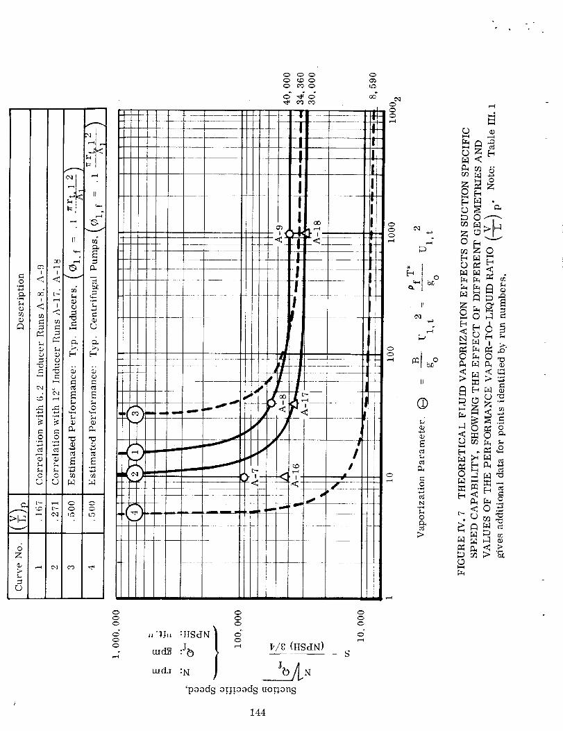
O(3
I I
• I r-_
•r-4 °,-_
.r-_ .F-4 I
0
>1_
d
ff--
b_
0 0
0 •
M M
L_ _ 0
0
L) •
_z_0
oN e.
M M'_
• _ "
•_, <o_
0
00
00
. "1,.T.
ttl ch_
tud._
000
:HgdN } o:N JbAN
'poad S a[jraad S uo.Bon 8
144
- S
0
00
a) Head coefficient
b)
c)
d)
If the loading is maintained light (equation IV. 24) the head coefficient in
a reasonable length will not be great. However, attention to maximum
possible deceleration criteria and diffusion factors are necessary to
prevent loss of control of the flow, (reference 33). In the interest of
restricting vapor Cavities to narrow regions, relative velocity diffusion
should probably be minimized while keeping losses to a minimum.
Inlet tip blade angle, Bb, t, 1
Feature (c) should lead to low blade angles throughout the inducer which
are shown to be necessary in other optimizations (references 7, 34 and 35).
Even with light loads, low B's are necessary. This is probably because
the incidence at high blade angles for reasonable leading edge loadings is
not sufficient to avoid the choking problem; i.e., i//_flow is probably
closely related (V/L)p for low angles. However, two problems arise ifis too low; viz., higher losses due to the low hydraulic diameter of
the resulting passage cross section, and a higher O with the consequentNPSH difficulties. This latter problem arises for a given fluid, mass
flow rate and rotative speed, because a lower blade angle requires a
higher inlet diameter and tip speed.
Incidence i
This difference between the blade and relative flow angle should be greater
than that required to compensate for blade blockage. The amount of incidence
should be sufficient to avoid choking the passage by vapor formation at too
high a value of NPSH. Too high an incidence is undesirable because of the
back flow and instability that develops especially at high NPSH, and because
of vapor formation arising from the attendant loading.
Solidity a, or length m.
A large solidity or inducer length is necessary to contain the two-phase
fluid in the front or leading portion of the machine• Liquid is required
at exit in order to obtain the pressure rise. Also, the blade loading
must be very light to prevent excessive vapor generation by reduced
pressure on the suction sides of the blades. The moment of momentum
relation shows both these points when expressed in the following form:
w d HiPp- Ps =
n b r 12b dm
where the ideal head H i = UV0/goin which mass flow rate w exists.
(IV. 24)
and b is the blade height of the passage
145

The computer programs for analyzing the three-dimensional flow field are probablynecessary to optimize these features successfully where two-phase flow with lossesis involved. The primary object of a design so evaluated is to avoid the chokingphenomenonas uniformly as possible in all sections of the inducer. The exact three-dimensional method has the capability of analyzing thermodynamic non-equilibriumcaseswith the appropriate changesin the loss and density expressions. If acceptable,the approximate methodwould be more easily adaptedto this problem simply byempirical corrections to the equilibrium loss factors.
146
CONCLUSIONS
We have obtained solutions to the set of simultaneous differential equations andboundary conditions required for a general continuumdescription of single and two-phasethree-dimensional flow with losses in turbo-pump inducers. Becauseof thisgenerality, both the exact and approximate methodsof solution that we developedarealso applicable to other turbomachines. Althoughwe used a thermodynamic equilibriummodel with empirical loss factors to accountfor the two-phase and loss effects, thisfeature of the analysis is purposely subject to changewithout destroying the basic systemof equationsor mathematical iterations.
The exact three-dimensional methodof solution successfully employed the total residualrelaxation conceptfor the simultaneous finite difference solution of four non-lineardifferential equations and the attendantboundary conditions and additional fluid equations.We obtained results for nine runs without losses, andthe concluding remarks at the endof Section II contain observations of the numerical and fluid dynamic phenomenain eachrun. Together, these empirically demonstrate the validity of the method. The first fiveruns were special cases for which knownanswers were available. These runs, whichdescribed both liquid and two-phaseaxial flow through paddle-wheel channels demonstratethat the relaxation procedure converges with goodresults. They also show that a largenumber of finite difference field points gives more accurate answers.
Of the four runs on the sample 6.2° and 12° variable-lead inducers, all were for in-compressible flow exceptone on the 12° machine. This one revealed that the inclusionof these two-phase effects required a negligible increase in computing time. Oneincompressible run on eachinducer gave reasonableoverall performance results evenwith the coarse, highly non-orthogonal grid that we used for these low-angle channels.The more detailed internal distributions differed from those obtained by simple radialequilibrium techniques, but were qualitatively reasonable. The distributions resultingfor the one special run with pressures forced to satisfy the streamline momentum equationfor no loss were more familiar. This showedthat reasonably accurate results arepossible with a grid that is too coarse for the relaxation procedure to produce low enoughresiduals to guaranteethem. The initial positions of the upstream and downstreamstagnation stream surfaces were not changedas the progress of the solutions indicatedthat some load existed on these extensionsof the blades. However, as one comparesthe differences in these runs, the inaccuracies of the coarse grid (e.g. 5 x 5 x 22) thatwe used (for reasonable computer running time) appear to have had more effect on theanswers. We have presented detailed recommendations at the end of Section H thatcontemplate satisfactorily accurate three-dimensional answers for lossless flow intypical inducers with a 10x 10x 50 grid, about twelve hours on goodcomputing equip-ment, and appropriate handadjustment of the blade extensions. Losses are easilyincluded and may require a finer grid and more time.
The approximate methodof solution was more rapid, but it employed assumptions thatamount to combining two quasi-two-dimensional solutions to get answers in threedimensions. However, it is a step forward because it does combine these solutions
147
with two-phase flow andloss effects. The method of solution by balancing initially-assumed streamline positions makes it possible to get satisfactory answers for avery small number of these streamlines. Results of over eighteen runs demonstratethe capability of this method as a rapid way of judging or grading an inducer; e. g.,by the results of several runs at various inlet conditions. This would determine ifandat what condition a particular inducer shouldbe analyzedfurther by the moredetailed andlengthy exact method. Abouthalf of these approximate runs containedtwo-phase flow with losses. The others were incompressible runs with and withoutlosses. This data clearly describes blade leading edgeunloading that occurs forcavitating conditions (low NPSH). In fact, several resulting inducer pressure-rise-versus-NPSH curves at different values of vaporization parameter showthat our modelfor these real fluid effects qualitatively produces the familiar headbreakdown curve.Stronger loss factors appear to be necessary to reproduce the shapeof this curvemore exactly; although"choked" or minimum NPSHconditions for complete headbreakdown correlate reasonably with test results. The basic restrictions of ourapproximate method may be partly responsible for this lack of complete correlation.
These results include the fluid and scale effects of the cavitation and thermodynamicvaporization parameters that are part of the analysis model. However, further studyshowsthat this data has some correlation with the well-known, simplified, vapor-to-liquid volume ratio theory for minimum allowable inducer NPSH. The fact that two-phasemotion exists with negligible inducer performance effects over a wide range ofhigher values of NPSHindicates that two cavitating regimes exist over the NPSHrange, viz., "unloading" and "choking". The simplified theory probably predicts thesefluid and scale effects as well as it doesby being of importance in only the chokingregime, which causes complete headbreakdownregardless of non-cavitating pressurerise.
This theory and data indicate that inducer designoptimization with these analysismethods can be doneby examining different designs for the effects of (a) headcoefficient,(b) inlet blade angle, (c) inlet incidence angle, and (d)blade solidity. Empirical modi-fications to the programs appear to be necessary to improve the existing thermodynamicequilibrium model for two-phase flow andloss effects. This may be sufficient todescribe the non-equilibrium phenomenaif they are not separately distinguishable inthe experimental test results that would be used for the purpose. Fortran IV listingsof both the exact and approximate analysesare included in this report, andthe programsare ready for further use.
148
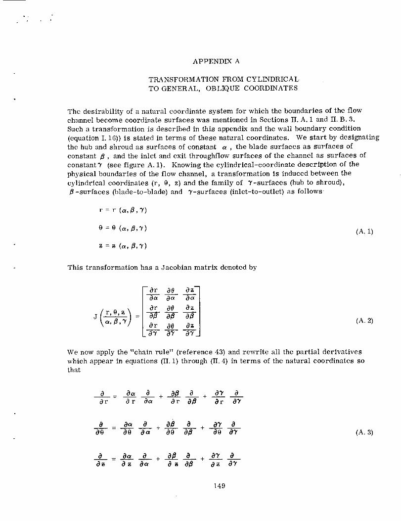
APPENDIX A
TRANSFORMATIONFROM CYLINDRICALTO GENERAL, OBLIQUE COORDINATES
The desirability of a natural coordinate system for which the boundaries of the flowchannel becomecoordinate surfaces was mentionedin Sections II. A. 1 and II. B. 3.Sucha transformation is described in this appendixand the wall boundary condition(equation I. 16)) is stated in terms of these natural coordinates. We start by designatingthe hub and shroud as surfaces of constant a , the blade surfaces as surfaces ofconstant fl, and the inlet and exit throughflow surfaces of the channel as surfaces of
constant'r (see figure A. 1). Knowing the cylindrical-coordinate description of the
physical boundaries of the flow channel, a transformation is induced between the
cylindrical coordinates (r, 0, z) and the family of "r-surfaces (hub to shroud),
fl-surfaces (blade-to-blade) and "r-surfaces (inlet-to-outlet) as follows
r =r (a,8,7)
0 -- 0 (a, fi,v)(A. 1)
This transformation has a Jacobian matrix denoted by
- Or O0 Oz7Oa Oa 3a
Or Ot_ O z
Or 08 az07 07 03'
(A. 2)
We now apply the "chain rule" (reference 43) and rewrite all the partial derivatives
which appear in equations (II. 1) through (II. 4) in terms of the natural coordinates sothat
O _ Oa a + _ O + 07 OOr Or Oa Or OB Or O_
O aa a aB 8 a'r a-- + +
O0 O0 aa 80 aB Oo a'r (A. 3)
0 _ Oa 0 + 0____ 0__0_+ O'r 08_ O z Oa 8 _ OB O_ 07
149
Constant
a) Crosseetional View
Shroud
___.__ J / J
Hub
b) Meridional View _
orD
/
#<
/
c) Developed View
FIGURE A. 1. NATURAL COORDINATE SURFACES FOR GENERAL
CHANNEL GEOMETRY.
150
q
Using the notation of equation (A. 2), we see that the nine coefficients in equations
(A. 3) are the elements of the Jacobian matrix
-0_ o_d_ 03"Or Or Or
o_ o_£ 0___L_O0 O0 ao
o_ o_g_ o__Z_ Oz O_ 0 _-
r,O,
r, 0,_which is the matrix inverse of J (a,T,_) (reference 44).
needed for the evaluation of O-%r' 0-_ and are calculable from
Oa _ ( O0 Os O0 0_ ) l-Or O(J 03" 03" O-b--fl- "-D
o____= (oo a_ 00 0_) 1Or _ _'--Td--'_- --ff
03"_ (00 o_ oo o_ ) xOr a_ a# oB Oa "_
Oa _ [ Ozao \ of�
o_K= ( o_O0 03"
03' _ [" OzaO _, Oa
Oa _ { OrO_ \ a f�
o__£ __( orO _ a7
03' _ (_OrOz Oa
]03" 03" O#
Or as Or \Oa 03" ]Or
1
-61
aa --ff
O_ Or _ 1-_ } --ff
1--6
1
--ff1
-6
j{ r,O,_ /
a] _5] is given by
a# a#O0 Or dO03" 03" 0t/ ]O0 Or O0aa aa -a_ )O0 Or O0 "_
of� of/ aa ]
where the determinant of
( ) Or O00z O0 0_)Or O0 O_ O0 O_ Or (00 as oo o_ +
D = _ --_ 07 03" Of/) + "_ k_O-_ Oa OY _(-_ O# Off 0-_
(A. 4)
Therefore, the nine coefficients
(A. 5)
(A. 6)
The main analysis program, described in Appendix C, uses formulae (A. 3) for calcu-
lating all the partial derivatives of the variables appearing in the residuals as given by
equations (II. 5) through (II. 8). The necessary transformation coefficients are calculated
by a subroutine from the (r, 0, z)-coordinates of the grid points using formulae (A. 5)
and (A. 6).
For a typical inducer channel the degree of obliqueness of the (a, B, _,)-system is
largely due to the blade angle. For example, at the blade leading edge of the 6.2 °
151

inducer channel, with which run E-6 was made, a typical "star" of grid points ishighly oblique becauseof the shallow blade angle. Figure A. 2 shows such a star nearthe blade leading edgeat the root-mean-square radius of r -- 0. 7454where the bladeangle is 8.4° (see equation (II. 40)). In the interior of the channel, where A_ is 0. 23524
instead of 0. 10857, the distance A_ is even greater relative to the distances Aa = Ar
andAB -- rA0.
This situation may be alleviated by taking the "r-surfaces to be quasi-orthogonal to the
blade surfaces rather than perpendicular to the z-axis. One drawback this has is that
many more _' -stations are required. Also, if the grid points do not lie on planes of
constant _, the determination of blade loadings and of throughflow boundary conditions
is rather difficult. A simpler remedy is to form a denser grid of points although this
increases computer time per relaxation cycle. We again point to the quality of our
results in Section II. B and recommend that for any particular channel geometry a
reasonable grid be selected based on qualitative diagrams similar to figure A. 2.
The treatment of the wall boundary condition
w. _ =o (i. 16)
is as follows:
At a point on a blade we can let the normal vector, "if, be VB because the blades are
surfaces of constant B • Thus
W. n = W • VB=0
or
u_-7+ +w =0r O0 Oz (A. 7)
Similarly, since the hub and shroud are surfaces of constant a, a normal vector at
such a point is V a and we have
U mOa + v Oa + w O---g-a=0Or r O0 O_
Since the hub and shroud are surfaces of revolution, i.e.
point the condition is
on a hub or shroud
u 0__ga + w 3--_a =0 (A. 8)Or Oz
At an "edge" point, i.e. where a blade meets the hub or shroud, equations (A. 7) and
(A. 8) must be satisfied simultaneously.
152

h_
<I
O0
Z_
_z<
Z _
Z_"_00
0 ozr_
m _
8 _
Z
g o0
153

In the computer program in its present form (see
(A. 8) are respectively solved for w and u, i.e.
Appendix C) equations (A. 7) and
OB + v OB_/O__ (A. 9)w=- (u 0--'-'r r 00
0o/U = -W'-_(A. 10)
Thus, on a blade surface w is explicitly dependent on u and v. On the hub or shroud u
is directly determined by w. This is because, for the blade angles we have been
considering, the dominant coefficients are 0B/ 0s and Oa/ Or. In fact, equations
(A. 9) and (A. 10) may be used successfully for blade angles and hub and shroud slopes
of up to 60 ° to 70 °. This method is used merely for convenience of programming --
every grid point has four residuals associated with it. To make the program completely
general with respect to channel geometry, equations (A. 7) and (A. 8) can be treated
as "boundary condition residuals", in which case there would be five residuals at
boundary points instead of the usual four (see Section II. C. 2).
Finally, the ( a, B , _" ) -surfaces need not be uniformly spaced as concerns the validity
of the transformation formulae. Thus, with a proper choice of these surfaces the grid
can be made denser in the boundary regions relative to the interior of the flow channel,
thereby achieving greater accuracy close to the boundaries where the discretization
discrepancy is the greatest (see Section II. A. 5).
154

APPENDIX B
COMPLEMENTARY STREAM FUNCTIONS
In this appendix are discussed the development and applications of a pair of comple-
mentary stream functions to the solution of the three-dimensional fluid flow problem,
as outlined in Section I. The advantages and disadvantages are weighed against each
other and it is concluded that, although the approach is aesthetically appealing, much
more development is required before it can be applied as a practical solution method.
Observe that a vector can always be represented as lying along the intersection of two
nonparallel planes (which are not necessarily orthogonal to each other). Specifically,
we can represent the relative velocity vector, W, at a point as lying along the inter-
section of two planes, each of which is tangent to one of a pair of surfaces at that
point. Designating two such families of intersecting surfaces as
# (r, 0, _) = constant 1
!a (r, 0, _)= constant
(B. 1)
yields (see figure B. 1)
W=A V#xVa (B. 2)
Here _ is some proportionality function whose nature can be determined by satisfying
the continuity equation as follows:
V. W= VX. (YpxVz)+ hr. (V#xVa)
= V'X. (VpxVv)
= :o
i. e. _ is constant along streamlines. Therefore _, is a function of # and _ only and,
hence, no generality is lost by taking }, as unity, or
W= Vp xVa (B. 3)
No rigorous treatment of the conditions under which such families of surfaces exist
is given here. Maeder and Wood (reference 11) simply assume their existence whereas
Yih (reference 10) derives them as solutions to the differential equations which describe
streamlines. Additional justification for taking _ as unity is given by Yih as well as byBenton (reference 45).
155

P
xv_
FIGURE B. 1. PORTION OF A STREAMLINE SHOWN AS THE CURVE OF
INTERSECTION OF A PAIR OF STREAM SURFACES.
156
For the case of a compressible (or two-phase) fluid, the above development is repeated
with the flux vector, P W, to obtain
W = VpxV_
One immediate advantage of this transformation is that the continuity equation is
satisfied identically because of
(B. 4)
V. (p W)= V. (VitxVa)=0
which is a vector identity. Also, the three velocity components are now expressed in
terms of two functions. Thus the problem is reduced to solving the resulting three
momentum partial differential equations for p, it and a.
Another advantage is the ease with which the wall boundary conditions are met.
portion of a wall boundary is considered as a surface of constant a, for example,
then a normal vector to this surface is given byVa. Thus
If a
W. n = 1-- VitxVa=O (B. 5)P
which is again a vector identity. Placing it or a surfaces on the boundaries, therefore
automatically satisfies the wall boundary condition. This is consistent with the
geometric interpretation of the it and a surfaces as stream surfaces. With this in
mind, we tried two systems of arranging these surfaces in the flow channel.
In the first system, the hub and shroud are _ -surfaces and the blades are tt -surfaces
(figure B. 2a). It is shown in reference 10 that the total mass-flux across an area
bounded by two pairs of surfaces such as a= al, a = a2, it = Pl, and p =//2 is given
by
w= 0/2-//1) (a2- al) (B. 6)
Thus, making the hub be a surface a= 0, the shroud a= WT and the blades p = 0 and
it = 1.0, satisfied mass-conservation in the large. This "natural" way of arranging
the stream surfaces does, however, prevent a streamline from crossing from a blade
onto the shroud, say; i.e. the "edges" of the channel are forced to be streamlines
themselves. How much of a drawback this is is not clear because the streamlines a
finite distance away from the boundaries can still produce the counterrotation observed
in typical inducer flows. On the one hand it is easy to show that a streamline which
touches an edge must at least be tangent to it at the point of contact. On the other hand,
in two-dimensional potential flow near a corner, fluid particles on the boundary do go
around the corner if the corner angle is obtuse*. We also foresaw possible numerical
* This example was brought to our attention by Doug Anderson of the Lewis Research
Center, NASA, Cleveland.
157

difficulties due to the "bunching" of stream surfaces near the boundaries resultingfrom the relative rotation of the fluid in the passage.
For these reasons we decidedto try another system of steam surfaces (figure B. 2b).In this system the entire channelboundary is made a a -surface of value _ = q, with
other a-surfaces nested inside. The p -surfaces radiate from the surface a = 0
(this degenerate surface is actually a curve) so that a typical cross section resembles
a spider web. With this system the question of streamlines moving across the edges
of the channel is immaterial. One very serious drawback is the singularity which
exists about the curve a= 0. We were unable to surmount the numerical problems
associated with this singularity in any practical way. A lesser disadvantage is the
discontinuity due to the coinciding of the surfaces _ = 0 and p = 1.0, similar to the
discontinuity which is present in an ordinary polar coordinate system where the rays
0 -- 0 and 0-: 2_ coincide. By use of a special algorithm which permitted the p -surfaces
in the vicinity of this apparent discontinuity to be two-valued, we were able to compute
p -derivates in the usual fashion.
The form of the governing equations is independent of which system of stream surfaces
is used. When the transformation (B. 4) is applied to the vector momentum equation
(I. 4) the result is
d d 1 dp
goVp+Vpx_-_7_-Vax _ _7/_--_- (VpxVa) dt
+ 2fl x (Vp x$'_) +pfl x (_xr) + pF(B. 7)
The three scalar components of this equation can also be obtained from equations (H. 1),
(II. 2) and II. 3) by substituting into them
U --
1 O_ 0¢ 0¢ OPrp ( O0 Oz O0 O_ )
1 O# Oz Oa Opv= _ ( 0_ Or 0_ Or ) (B. 8)
1 OP Oa Oa OP }w= r--P ( Or O0 Or O0
which are merely the components of equation (B. 4).
The resulting scalar equations contain pure as well as mixed second order partial
derivatives of p and a. The typical star of grid points for the corresponding finite-
difference equations would contain 19 points instead of the seven points we are now
using (figure H. 2). The drawbacks of this are apparent.
158

a---w T
--p--- 1.0
a) "Quasi-Orthogonal" System
p 0
p:= 1.0
b) "__Spider Web" System
FIGURE B. 2. TWO ARRANGEMENTS OF p- and a-SURFACES
159

We felt that the above-mentioneddifficulties made the use of these complementarystream functions an impractical approach at the present, compared to the directnumerical solution of the untransformed equations as presented in this report. Werecommend, however, that the use of these (p,a) -surfaces be investigated further,
because, with the use of differential geometry, they may lead to a rigorous analysis of
the throughflow boundary conditions needed for the general three-dimensional problem
in turbomachinery.
160
APPENDIX C
INSTRUCTIONS FOR USE OF
EXACT SOLUTION COMPUTER PROGRAMS
The main analysis program for the exact solution method (see Section II. A. 3) and
the accompanying data reduction program (see Section II. A. 6) are described in this
Appendix. Both programs are written in Fortran IV. Their inputs and outputs
are described, followed by their respective Fortran listings. In the case of the main
program a block diagram is included.
a) Main Analysis Program
The main program and its five subroutines have a common storage requirement of
39,638 locations. The running time per relaxation cycle can be estimated as in the
following example:
For a 5 x 5 x 22 grid there are 1585 independent discrete variables (see
equation (II. 14)). For M=3, a maximum of six values of R* will have tobe calculated for each of these variables (see Section II. A. 3) making a
maximum of 9510 star residuals to be computed during one relaxation
cycle. A UNIVAC 1107 can calculate approximately 40 star residuals per
second, this having been established experimentally. Thus it would take
at most 238 seconds, or four minutes for each relaxation cycle.
The input to the program consists of the cylindrical (r, 0, z) -coordinates of the
selected grid points, certain numbers which control the nature of the relaxation
processs, information describing the fluid, and initial values for the field of velocity
components and pressures. A definition of these input quantities follows. For the
exact format in which these inputs are to be given, please see the corresponding
Fortran listing.
IMAX, JMAX,KMAX:
The number of radial (hub-to-shroud), circumferential (blade-
to-blade) and throughflow (upstream-to-downstream) grid stations,
respectively. I= 1 on the hub andI= IMAXonthe shroud; J= 1
on the pressure (driving) blade surface and J = JMAX on the suction
(driven) blade surface; K -- 1 on the upstream throughflow boundaryand K = KMAX on the downstream one.
KLE, KTE: The K-index of the axial stations corresponding, respectively, to
the blade leading and trailing edges.
R(I, J, K): The radial coordinates, r, or the grid points.
T(I, J, I_: The circumferential coordinates, 0 (in radians), of the grid points.
161

Z(I, J, K): The axial coordinates, z, of the grid points.
TITLE: Any type of run identifying information which may consist of up to80characters (including blank spaces). Noneof this informationis processedby the computer.
KOUNT: The number of the first cycle of the current run (for "book-keeping"
reasons only).
NUM: The number of relaxation cycles to be executed by the current run.
If NUM = 0, no relaxation is performed: All residuals and the
overall RMS value are computed and the regular output is presented.
M. The number of adjustment magnitudes to be tried with each variable
(see Section II. A. 3). Recommended: M = 3.
NSEQ(1),
NSEQ(2),
NSEQ(3),
NSEQ(4):
The sequential order in which the four variables are to be adjusted
at each grid point where the four variables are identified by the
computer as follows: uis 1, vis 2, wis 3 andpis 4. Thus, for the
recommended sequence (see the discussion following Run E-6 in
Section H. B. 3), NSEQ(1) = 4, NSEQ(2) = 3, NSEQ(3) = 2, NSEQ(4) = 1,
resulting in an adjustment of sequence of (p, w, v, u).
DMAX(1),
DMAX(2),
DMAX(3),
DMAX(4):
The four starting trial adjustment magnitudes 5u, Sv, 6w, Sp,
respectively (see Section II. A. 3). Recommended: DMAX(1) =
DMAX(2) --DMAX(3) = DMAX(4) = 0.i.
A: The successive adjustment ratio,
Recommended: a = 0.1(see Section H. A. 3).
CRIT:
E:
The accuracy criterion, such as the quantity It 2 rt ' 1
The convergence parameter, ,, of equation (H. 19).
of equation (II. 19).
REV, DLIQ,
PSAT, TT,
VISC:
The values of rotative speed, l_, liquid density, Pf/go, saturation
pressure, Psat, vaporization constant, T*, and kinematic viscosity,v , respectively.
U(I, J, K): The values of radial velocity, u, at each grid point.
v(I, J, K): The values of relative circumferential velocity, v, at each grid point.
W(I, J, K): The values of axial velocity, w, at each grid point.
P(I, J, K): The values of static pressure, p, at each grid point.
This completes the list of input quantities.
162
The output of the program consists of punchedand printed output. After executingNUM relaxation cycles the entire list of quantities, starting with TITLE, is punchedonto cards in exactly the same format and order as for the corresponding inputs.The values of NUM, DMAX(1), DMAX(2), DMAX(3), DMAX(4), U(I, J, K), V(I, J, K),W(I, J, K) and P(I, J, K) are the latest values. Thus the punchedoutput of one runmay be used to continue the same run at a later time without having to rerun therelaxation cycles of the first run.
The first line of the printed output consists of the entire contents of TITLE, therebyproviding any desired way of identifying the computer run. The size of grid isidentified next, followed by the values of M, a, _,Pf/go, Psat, T* and v. Then the
sequence in which the variables are adjusted, is stated, rhe next portion of the
printed output concerns the cycle-by-cycle progress of the relaxation scheme. It
is printed in columns with the following headings:
RE LAX
CYCLE:
The sequential number of each relaxation cycle, the first cycle
of the current run having the number KOUNT as given in the
input.
NO. OF
TRIES:
The total number of trial adjustments that were made during each
cycle. Note that this number cannot exceed 2 x M x D, where D is
given by equation (II.14).
TOTAL RMS
RESIDUAL:
The root-mean-square value of all residuals in the entire grid
of points.
MAX. RMS
RESIDUAL:
The largest root-mean-square value of the four point residuals
as given by equations (II. 5) through (II. 8).
MIN. RMS
RESIDUAL:
The smallest root-mean-square value of the four point residuals
as given by equations (II. 5) through (II. 8).
M AGNITUDE
OF BIGGEST
ACCEPTED
ADJUSTMENT
FOR U, V, W, P:
The magnitudes of the largest adjustments _u,
were accepted during each cycle.
6v, Sw and Sp which
The last portion of the output presents the latest values of the variables at all grid
points. This information is printed in columns with the following headings:
I,J, K The three indexes of each grid point. Recall that I -- 1 on the hub
and I = IMAX on the shroud; J = 1 on the pressure (driving) blade
surface and J=JMAX on the suction (driven) blade surface; K = 1
on the upstream throughflow boundary and K = KMAX on the
downstream throughflow boundary.
163

U: The radial velocity component, u.
V: The relative circumferential velocity component, v.
W: The axial velocity component, w.
P: The static pressure, p.
D: The point density, p/go"
RES: The sum of the squares of the four point residuals, as given
by equations (II. 5) through (H. 8).
The program will continue until either the largest root-mean-square of the four point
residuals is less than CRIT times E (see equation II. 19) or until NUM relaxation
cycles have been executed. Accordingly, the message "CONVERGED" or "MAXIMUMNUMBER OF CYCLES EXECUTED" will be printed on the output sheet. In either case,
the computer will stop with an input tape end-of-file condition.
b) Data Reduction Program
The Data Reduction Program and its two subroutines have a common storage require-
ment of 23,757 locations. A UNIVAC 1107 requires between 25 and 30 seconds to
reduce the data of a 5 x 5 x 22 grid.
The input to the Data Reduction Program is identical to the input to the Main Analysis
Program. Thus, the input describing the grid point coordinates can be combined with
the punched output of any given run of the Main Analysis Program to form a complete
input set for the Data Reduction Program.
The first line of the output consists of the entire contents of TITLE, thereby giving
the reduced data exactly the same identification as the corresponding main analysis
run. The second line identifies the number of the relaxation cycle whose results are
being reduced. Next, a station-by-station listing is given of hub-to-tip distributions
of quantities which are area-averaged over annular regions on each axial station. The
column headings are:
AXIAL
STATION:
The _ -value of each station. The stations corresponding to the
blade leading edge (K = KLE) and trailing edge (K = KTE} are so
designated.
RADIA L
STATION: The mean r-value of each annular region.
RADIAL
VELOCITY: The area-averaged value of V r.
164

TANGENTIALVELOCITY:
AXIALVELOCITY:
STATICPRESSURE:
DENSITY:
The area-averaged value of [email protected]
The area-averaged value of VZ.
The area-averaged value of p.
The area-averaged value of P/go"
This is followed by a station-by-station listing of the hub-to-tip distributions of
blade-to-blade pressure loadings, calculated simply as
Ap -- pp - Ps
The first column lists the values of z and the remaining columns (read from left to
right) list the hub-to-tip values of Ap for each annulus.
The last portion of the output gives the following mass-averaged, overall performance
parameters:
Inlet and exit pressure head: _ as calculated from equation (II. 26).
Inlet and exit absolute velocity head: 1/2 V 2, _as calculated from equation (II. 28).
Total head rise: AH, as calculated from equation (II. 30).
Shaft power per channel: Ps, as calculated from equation (II. 31).
Overall efficiency: y , as calculated from equation (H. 32).
Mass flow rate per channel: w T, as calculated from equation (II. 27).
This program will also terminate with an input tape end-of-file condition.
165
Read: Grid PointCoordinates
1_alculate
{ aACO___BBian\ Coefficients_(eq's A. 5)
1/
Read:
TITLE
99
tRead: KOUNT,NUM, M, NSEQ (1)....NSEQ(4),_u, Sv, _w, _p, a,
CRIT, e
I/Read: l_ ,
Pf
_oo' Psat'T*' v
"Read: Initial
Velocities &
Pressures
_pCoa_tul:t_] tA:_s_
_,X (eqI'7) J
FIGURE C. 1
450
A(/ADSjequentially
ust Local _
IV---_riables Except I
IWhere Fixed by]
_Boundary /_ Conditions J
IIIII
Calculate t
Local STAR
Residual:
R*i,j,k (eq II.16
"DO LOOP"
YES
1fOUTPUT
_k, ROUTINE )
Calculate All_int RESIDuals ]
"_ (eq's II. 5-8)J
360
/k=2 D°F°r \•., KMAX\
--\]=1,... ,JMAX ]-----
...
I Caleulate
Root-Mean-Square_ Residual
(eq's II. 15 & 18)
561 l 562
Initialize
_u, _v, 6w, Sp
for Next Cycle
YES
a) BLOCK DIAGRAM FOR MAIN ANALYSIS PROGRAM
(Numbers above boxes refer to key Fortran statement numbers in the
main program)
166

UbroutineESID
FIGURE C. 1 (Continued)99
Satisfy Wall BoundaryConditions:eq _. 9 on bladeseq A. 10on hub, shroudeq's A. 9 & 10 at "edges"
351
Calculate AllDerivatives:
0 0 008'
367
Convert All Derivatives to
Cylindrical Coordinates:0 0 0
Or' O0 ' 3_
(eq's A. 3)
385
I Calculate Loss
Terms:Fr, F0, F_
(Only if v¢ 0)
L 391
Calculate Point
Residuals:
R1, R2, R3, R4
(eq's II. 5-8)
RES (I, J, K)=
RI2 + R22 +
R32 + R42
b) BLOCK DIAGRAM FOR SUBROUTINE "RESID"
(Numbers above boxes refer to key Fortran statement numbers in the
subroutine)167

FIGURE C. 1 (Concluded)
_Dbroutine)---"
445
Restore LocalVariables andAffected Residualsto Original
TemporarilyStore Values ofthe SevenAffectedResiduals
RHLD = R'i, j, k NOTE: The symbol "x"stands for u, v,DX= 6xworp.
HX = xi, j,k
l
I _ "DO LOOP"
Do M times
I
42o
Ixi, j k=HX+DX _- 1' i
I Ii I
421
Recalculate 1 432 433
Residual:L°calStar _ J,k LR'i, DX = -DX DX = -aDXValues
(eq If.16)
430 /_ _ I
YES Y2 / _s _ N2_1
c) BLOCK DIAGRAM FOR SUBROUTINE "ADJ"
(Numbers above boxes refer to key Fortran statements in the subroutine)
168

C
C
C
CC
C
C
TABLE C. 1
FORTRAN IV LISTING OF EXACT ANALYSIS COMPUTER PROGRAM
THREE-DIMENSIONAL FLOW ANALYSIS FOR ROTATING CHANNEL
OF ARBITRARY ROUNDARY SHAPE
USING METHOD OF STAR RESIDUALS IN TERMS OF
RELATIVE VELOCITY COMPONENTS AND PRESSURE
TRW ACCESSORIES DIVISION, CLEVELAND 6AUG65
9 'i)
DIMENSION TITLE(16)
COMMON U(10•10,22),
1 DIlO,lO•22),R(10,1
2 DELXI4I.NSEQ[4],AZ(10,IO,22)•BR(]O
4 CTIlO•IC.22).CZ(]O
5 IRSTAR,DX,I,J,K•II
READ 1001 ,
READ 1008•
READ 1008
READ 1 ,?,C)8 ,
CALL JACOBREAD 10OO,
PRINT IG04,
READ i001 •
READ 1002 ,
READ 1002 ,
READ 1 ()02,
READ 1002 ,READ 1002,
I'_AX.JMA
(((RCI
({ITIIlCIZ(I
VI]O,IO,22),WIIO,IO,22)•P(IO,IO,22)'
O,22),TIIO,IO,22),ZIIO,tO,22),FR,FT,FZ,DMAX(4}'
RES(IO,I0,22),ARI]0•IO,22),AT(IO•]O'22)'
•IO,22),BTI]O,IO,22),BZ(I_,IO•22),CR(1_•]_,22)_
•10,22),XH,RSTAR,TT,PSAT,DLIQ,REV•A,M*NVAR•NTR,
•JJ,KK•IMAX,.JMAX,Kr.'AX,VISC,NBO,KLE•KTE
X,KM4X•KLF,KTE
,J.K)•I=I,IMAX) •J=].JMAX),K=I.KMAX)
.J•K),I=] .IMAX).J=],JMAX),K=I•KMAX)
.J.K).I=I.IMAX),J=I.JMAX).K=I,KMAX)
TITLE
TITLEKOUNT,NUM•M,(NSEQ(
(DMAX(LI.L=I•A}•A.
REV,DLIQ,PSAT
(Ill;II.J,K).I=I
(((V(I,J,K),I=I
(((W(I,J,K),I=I
REA.) 1002, (((PII•J,K).I=I
NMAX=KOIINI +NEJMPRINT 1007, iMAX,J%AX,KMAX,M,
PRINT 1006. (NSEQ(L}.L=I.4)
NTR=O
ANR = 4*IMAX_JMAX_KMAX
DO 150 L=I•4
150 DELXIL)=DMAX(L)CALCULATE POINT DENSITIES
DO 501 K=I,KMAX
DO 50] J=I,JMAX
DO 591 I=I,IMAX
IF(TT}502,503.502
5(32 CALL STATE
GO TO 501
503 D (I,J•K)=DLIQ
501 CONTINUE
CALCULATE ALL POINT RESIDUALS
NBD=I
DO 350 K:I•KMAX
DO 350 J=I•JMAX
DO 350 I:I,IMAX
IF(D (I,J•K))500.500,500
5o0 CALL RESID_50 CC)NTINIIE
PRINT 1012CALCULATE TOTAL ROOT-MEAN-SQ_JARE
467 RT=O.O
RESMAX = 0.0
RESMIN = RES(1,1.I)
DO 368 K=I,KMAXDO 368 J=],JMAX
DO 368 I=I,IMAX
L)•L=I,4)
CRIT,E
,TT,VISC
• IMAX) ,J=I,JMAX}•K=] •KMAX)
• IMAX) ,J=I..-;MAX).K=I,KMAX)
.IMAX) _.J=] .JMAX) _.K=I ,KMAX)
,!MAX) .J=I,JMAX},K=],KMAX}
A,REV,DLIQ,PSAT,TT,VISC
RESIDUAL
169

402
403
404
368
1_1
370
IFIRESII,J,KI-RESMAX}403,403,402
RESMAX=RESII,J,K)
SO TO 36PIF(RES(I,J,KI-RESMIN)404,368,368
RESMIN = RES(I,J,K)
RT=RT+RES(I,J,K)
RMS = SQRT(RT/ANR)
RESMAX=SQRT(RESMAX/4.)
RESMiN=SORT(RESMIN/4.}
PRINT 1013, KOUNT,NTR,RMS,RESMAX,RESNIN,(DMAX(L),L=I,4)
DO 151 L=1,4
DMAX(L}=O.O
IF(RESMAX'CRIT*E)369,369,370
KOUNT=KOUNT+I
NTR=O
IF(KOUNT-NMAX)360,360,371
C-START SUCCESSIVE VARIATIONS
360 DO 460 KK=2,KMAX
DO 460 JJ=I,JMAX
DO 460 II=I,IMAX
IRSTAR=I
CALL STAR
DO 460 L=1,4
NVAR=NSEQIL}
GO
111 IF
611 IF
222 IF
481 IF
482 IF
533 IF
485 IF
471 IF
472 IF
486 IF
487 IF
450 CAL
46¢ CON
DO
IF
561
CYCLE
TO (lll,222,33_,450),NVAR
KK-2)46h,46P,611
(II-1)w(IMAX-II))460,460,450
KK-2}46n,&6_,481
KK-K_AX)450,482,460
(JJ-I)_(J_AX-JJ))460,460,450
KK-2)460,48_,486(JJ-1)*(J#AX-JJ))460,460,47]
(II-l)*(IMAX-II))460,472,450
AZ(II,JJ,KK))460,450,460KK-KMAX)487,460,460
(JJ-!)_[JMAX-JJ))460,460,450
L ADJ
TINUE
153 L:I,4
(DMAX(L)] 561,562,561
562
153
C
98
DELX(L)=DMAX(L}
GO TO 153
DELX(LI=DELXIL}*A
CONTINUE
GO TO 467
_** OUTPUT ROUTINE
PUNCH 1000, TITLE
KOUNT=KOUN[-I
PUNCH i001,
PUNCH 1002,
PUNCH 1002,
PUNCIt lOS,2,
PUNCH 1002,
PLJNCIt i'502,
PUNCtt ICO2,
PRINT 1004,
DO 97 K=I,K_IAX
PRINT 1005
KOIJNT ,NUM, M, (NSEQ (L ),L = I, 4 )
(DFL. X(L},L=I,4I,A,CRIT,E
REV,DI_ IQ, P_AT,TT ,VISC
(((!J(I,J,K),I=I,IMAX},J=I,JMAX},K=],KMAX)
( ( (V( I ,J,K }, I =1 , IHAX ) ,J=] ,JMAX } ,',<=I,KMAX )
( ( (W (I ,J,K ), I =] , IHAX ) ,J=1 ,JMAX ) ,K= I ,KMAX }
(((P(I,J,K),I=I,IHAX) ,J=I,JMAX),K=I,KMAX)
TITLE
97 PRINT 1003, ( (I,J,K,U(I,J,KI,V(I,J,K),WII,J,K),P(I,J,K),F)(I,J,K)
1 ,RES( I ,J,K} , I=I , IMAX } ,J=I,JMAX)
170

GO TO369 PRINT
GO TO
371 PRINTGO TO 9l(ll_
1000 FORMATI00] FORMAT
1002 FORMAT
1003 FORMAT
I004 FORMAT
I005 FORMAT
llHD, 1
1006 FORMATI
IW IS 3, P
1007 FORMAT( 13,
1 5H REV=, 12 lPE10.,'4,5X
1098 FOR,VAT(lP6E1012 FORMAT I6H R
1 71_,MIN RMS,
2 6H CYCLE,3
3 13X,1HP/)ICJI? FORMAT( 16,1
1014 FORMAT(/20X
](315 FOR_,'AT ( /2(_X
EN r)
991014
981015
8
INPUT-OUTPUT
16A512613}
8F10.7)
313,1P6EI8.6)
IGA5///)
FORMATS
II2X,IHI,2X,IHJ,2X,1HK, 9X,1HU,17X,IHV,17X,IHW,17X,1HP,17X,
5X',_HRES/ ]
2X23HADJUSTMENT SEC, UENCE IS ,411,38H WHERF U IS 1,, V IS 2,,
IS 4.//I)IHX,12,1HX,12,SH GR ID,GX,2HM: , I 2,6X,2HA:, IPEIO.411PE ] 0.4,5X, 5:tDL IQ= , lPEI O. 4,,5X , 5HPSAT: , lPEIO.4,SX , 3H TT = ,
,_HVISC:,IPElO,41)
1_.7)E:LAX,3X,SHNO OF,SX,gHTOTAL RMS,TX,THMAX RMS,7X,
16X,44HMAGNITUDE OF BIGGEST ACCEPTED ADJUSTMENT FOR/
X,5HTRIES,3 (6X,8HRESII)UAL) , 17×,IHU, 13×,1HV,13X ,]HW,
8,1PBE14-4,8X,IP4EI4.41
,OHCONVERGED/]
,_HMAXIMfJM NUMBER OF CYCLFS EXECIITEDI)
171

SUBROUTINEJACOBCALCULATION OFt JACOBIAN COEFFICIENTSCOORDINATETRANSFORMATION
FOR GENERAL-TO-CYLINDRICAL
]6
COMMON U(IO,10,22),V(IO,10,22),W(IO,IO,22),P(IO,lO,22),
I D(IO,10,22}.R(IO,10,22).T(10,10,22),ZIIO,IO,22),FR,FT,FZ,DMAX(4}'
2 DELX(4).NSEO(4). RES(IO,IO,22),AR(IO,10,22),AT(IO,IO,22),
3 AZ
4 CT
5 IR
DO
DO
DO
IF
RA
TA
ZA
GO
4 IF
5 RA
TA
ZA
GO
6 RA
TA
ZA
I IF
8 RB
TB
ZB
GO
9 IF
10 RB
TB
ZB
GO
11 RB
TBZB
12 IF
13 RC
TC
ZC
GO
14 IF
15 RC
TC
ZC
GO
RC
TC
ZC
17 D
(I0,I0'221'BR(I0'I0'221 ,BT(IO,IO,22)'BZIIO'IO'22)'CR(IO'IO'221'
(I0,I0,22),CZ{ lO,IO,22}'XH'RSTAR'TT'PSAT'DLIO'REV'A'M'NVAR'NTR'
STAR,DX,I,J,K,II'JJ'KK'IMAX'JMAX'KMAX'VISC'NBD'KLE'KTE
18 K=I,K_AX!8 J=I,JNA×
18 I=I.IMAX
(I-i)3,3,4
= R(I+I,J,K)-R(I,J,K)
= T(I+I.J.K)-TII.J.K}
= "Z( I+I.J,K )-Z( I .J.K}
TO 7
( I- IMAX }5,6,6
= (R( I+I.J,K)-R( I-I ,J,K) )/2-
= (T( I+] .J.K )-T(I-I,J,K) )/2.
= (Z ( I+l .J,K }-Z ( I-] ,J.K) )/2.
TO 7
= R(I,J,K)-R(I-I.J,K)
= T(I,J,K)-T(I-I.J,K)
= Z(I,J,K}-Z(I-],J,K)(J'-I)8,8,9
= R(I,J+I,K)-R(I,J,K)
= T(I.J+I.K)-T(I.J.K)
= Z(I.J+I,K)-Z(I.J.K)
ro ] 2
(J-JMAXIIO,] l,ll
: (R( I .J+l .K)-R ( I .J-I,K) }12.
= (T( I .J+!.K)-T( I.J-] ,K) }/2.
= (Z( I .J+I,K)-Z (I .J-I.K) }/2.
TO 12
= R(I,J,K)-R{I,J-I.K}
= T(I,J,K}-T(I.J-I.K)
= Z(I,J,K)-Z(I.J-1,K)
(K-I)13.13.]4
= R(I,J.K+II-R(I,J,K)
= T(I,J.K+I)-T(I.J.K)
= Z(I.J.K+])-Z(I,J,K)
TC 17(K-KMAX }15,16,16
= [R ( I ..J.K+I )-R ( I ,J,K-I ) )/2.
: (T( I .J,K+] )-T( I ,J,K-] ) )/2-
-- (Z(I.J.K+I)-Z(I.J.K-]))/P.
TO 17
: R(I,J,K)-R(I,J,K-I)
= T(I,J.K)-T( I,J,K-I}
= Z(I J,K)-Z(I.J.K-1)
= RA*( B_ZC-TC*ZB)+RBW(TC*Z A-TA*ZC)+RC_(TAWZB-TBWZA)
AR ( I ,J ,K
BR ( I ,J ,K
CR ( I .J ,K
AT( I .J.K
BT( I .J ,K
CT(I,JtK
AZ(I,J,K
BZ(I.J,K
= TBwZC-TC*ZB
: TC_ZA-TA*ZC
= TAwZB-TRwZA
= ZEwPC-ZC*RB
= ZC*RA-ZAWRC
= ZA_RB-ZB*RA
= RB_TC-RC_TB
= RC*TA-RA*TC
/D
/D/D
/D
/D/D
/D
/D
172

18 CZI [,J,F-,)=IRA*TB-RB*TAI/DRETURN ....END
/ i
173
S
C-REDUC
C
1
2
3
UBROUTINE ADJ
TION OF TOTAL RESIDUAL BY SUCCESSIVE VARIATIONS OF U, V, W, P
OMMON U(IO)IO,22),V(IO)IO)22),W(IO,IO,22),P(IO)lO,22) )
D(IO,IO,22),R(10,10,22),T(IO,10)22),ZIIO,IO,22),FR)FT,FZ,DMAX{4)'
DELXI4),NSEO(4) , RES( I0,I0,22 } ,AR(I0,I0,22) ,AT( 1n,]0,22 ) ,
AZ (I0, i0,22) ,BR( ] q,I0,22) ,BT(10,10,22) ,BZ(10,10,22) ,CR( I0,10,22 ) ,
4
5
C U RR E hiT
HI=RES
H2=RES
H3=RES
H4=RES
H5=RES
H6=RES
H7=RES
CT ( I0 , 19,22 ) ,CZ ( I0, i0,22 ) ,XH ,RSTAR ,TT ,PSAT ,DL IC, REV ,A ,M ,NVAR ,NTR,
IRSTAR,DX, I ,J,K, I I ,JJ,KK, IMAX ,JMAX ,KMAX,V ISC, NBC),KLE,KTE
QUANTITIES TEMPORARILY STOREDVALUES OF ALL AFFECTED
II,JJ,KK)
II-I,JJ,KK)
II+I,JJ,KK)
II,JJ-I,KK)
II,JJ+I,KK)
II,JJ,KK-I)
II,JJ,KK+I)
RHLD=RSTAR
DX=DELX(NVAR}
HU=U(II,JJ,KK)
HV=V(II,JJ,KK)
HW=W(II,JJ,KK)
HP=P(II,JJ,KK}
HD=D(II,JJ,KK)
C-SUCCESSIVELY APPLY TRIAL VARIATIONS TO
5 DO 480 MA=I,M
420 'SO [0 (422,423,424,425),NVAR
422 U(II,JJ,KK)=HU+DX
GO TO 42]
423 VIII,JJ,KK)=HV+DX
50 TO 421424 W(II,JJ,KK)=HW+DX
GO TO 421
425 P(II,JJ,KK)=HP+DX
IF(TTI461,421,461
461 I=II
J=JJK=KK
CALL STAT_
42L NTR=NTR+]
IRSTAR=2
CALL STARIFIRHLD-RSTARI430,430,431
431 IF(ABS(DX}-DMAX(NVAR))457,457,920
920 DMAX(NVAR)=ARS(DX)
GO TO 457
430 IF(DX)433,457,432
432 DX=-DXGO TO 420
433 DX=-A*DX
480 CONTINUE
C-RESTORE ALL AFFECTED QUANTITIES TO ORIGINAL
!;(II,JJ,KK)=HU
V(II,JJ,KK)=HV
W(II,JJ,KK)=HW
P(II,JJ,KK)=HP
D(II,JJ,KK)=HD
44_ RSTAR=RHLD
RES(II,JJ,KK)=H!
IF(II-I)446,446,447
447 RES(II-1,JJ,KK)=H2
U, V, W, P
174
VALUES

446449
448
451
450
453
452455
454
456
457
IF(II-IMAXI449,448,448RES(II+I,JJ.KKI=H3
IFCJJ-I)450,450,451
RES(II.JJ-1,KK)=H4IF(JJ-JMAX)453.452,452
RESIII,JJ+I,KK)=H5
IF(KK-]}454_4549_55
RES(II,JJ,KK-I)=H6IF(KK-KMAX)456,457_457RES(II,JJ,KK+I)=H7RETURN
END
175

SUBROUTINE DLOSSCALCULATION OF LOSS TERMS IN MOMENTUM EQUATIONS
COMMON U(10,IO,22),V(10,10,22),W(10,IOt22),P(10']0'22)'I D(IO,10,22),R(10,IO,22),T(10,10,22),Z(10,10,22),FR'FT'FZtDMAX(4)'
2 DELX(4),NSEQ(4), RES(IO,IOI22),AR(IO,IO,22)tAT(10,IO'22)'
3 AZ(lO,IOt22),BR(]N,IO,22),BT(]O,10,22),BZ(IO,IO,22)tCR(10'IO'22)'4 CT(10,IO,22),CZ(10.10,22),XH,RSTAR.TT.PSAT,DLIQ,REV'A'_'NVAR'NTR'
5 IRSTAR,DX,I,J.K.II.JJ.KK,IMAX,JMAX,KNAX,VISC.NBD'KLE'KTE
FR=C.O
FT=O.O
FZ=O.G
RETURNEND
176
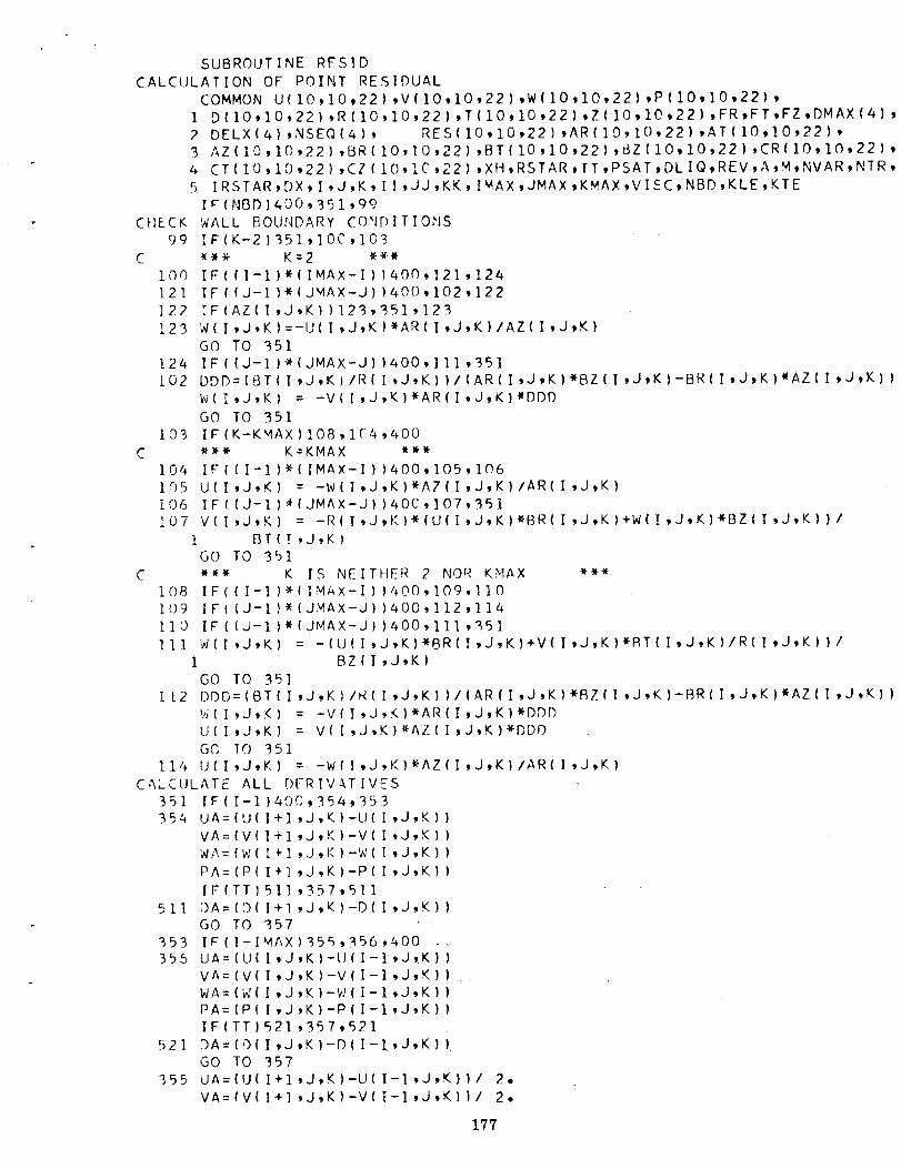
SUBROUTINE RESID
CALCULATION OF POINT RESIDUAL
COMMON U(lO,lOt22),VI10910,22),W(lO,lO,22)_P(lO,lO,22),
1 DI10,10,22),R(10,10,22),T(10,10*22),Z(10,lO,22),FRtFT,FZtDMAX(4)'2 DELX(4),NSEQ(4), RES(lO,10,22),ARI]O,lO,22),AT(10,]O,22),
3 AZIlO,lO,22),BR(10,10,22),BTI10,lO,22),BZI10,10,22)_CR(lO,lO*22)'
4 CT(lO,lO,22),CZ(lO,1C,22),XH,RSTAR,TT,PSAT,DLIQ,REV,A,M,NVAR_NTR'
5 IRSTAR,DX_I,J,K,II,JJ,KK,IMAX_JMAX,KMAX,VISC,NBD,KLE_KTE
IF(NBD1400,351_99
CHECK WALL BOUNDARY CONDITIONS
99 IF(K-2)B51,lOC,IOB
C _*_ K=2 *_*
100 IFIII-II*IIMAX-II}400,]21,124
121 IF(IJ-I)*(J_AX-J))400,102,]22
]22 [F(AZ(I.J.K}}123.351.123
123 W(I,J.K)=-U(I,J,K)WAR(I,J,K)/AZ(I,J,K)
GO TO 351
124 IF((J-]I_(JMAX-J))400.]11.351
tO2 DDD=(BT(I,J.K)IR(I,J.K))I(AR(I.J,K)*BZ(I,J,K)-BR(I,J,K)WAZ(I'J'K}}
W(I.J,K) = -V(I,J,K)WAR(I,J,K)WDDD
GO TO 351
tO3 IF(K-KNAX)108,1C4,400
C __* K=KMAX __
104 IF((I-I)*(IMAX-I))400,105,106]05 U(I,J,K) = -W(I*J,K)*AZII,J,K)/AR(I,J,K)
i06 IF(IJ-I)4(JNAX-J)}400,]07,351
107 V(I,J,K) = -R(I,J,K)*(U(I.J.K)_BR(I.J,K)+W(I.J.K)*BZ( ,J,K))/
1 BT(I.J,K)
GO TO 351
C .ww K IS NEITHER 2 NOR KMAX ***
IF((I-I)*(INAX-I)I400,109,IlO
IF((J-I)_(J_MAX-J))400.112,]14
IF({J-I)W(JMAX-J))4OO,I]I,q51
IO8
109
iI 0
111 W(I,J,K) = -(U(I,J
1 BZ(I.
GO TO 351
tl2 DDD=(BT( I,J,K)/R( I
'.';(I,J,K) = -V(l,J,
U(I,J.K) = V(I.J.K
GO, TO 351
114 U(I,J,K} = -W(I,J,
ALL [)FR I V-\T IVr_
IF ( I-1 )40C ,354,353UA:(U I+I,J,K)-U( I
VA=(V I+I,J.K)-V( I
WA=(W I+I,J,K)-W(I
PA=(P I+I,J.K)-P(I
IFITT 51] .357.511
,K)*BR( I ,J,K}+V( I ,J,K)WRT ( I ,J,K)/R( ,J,K))/
J.K)
CALCULATE
351
354
I.J.K)-V{I-]
I.J.KI-W(i-I
I.J.K}-P(I-I
521,357,52]
I,J,K)-D(I-1
357
,J,K}IIIAR(I,J,K)WRZ(I,J,K)-BR(
K}*AR(I.J,K)*DDD
)*AZ(I,J.K)WDDD
K)_AZ(I,J,K}/AR(I,J,K)
,J,K))
,J,K)),J,K))
,J,K})
51l DA=(D I+I,J,K)-D(I,J,K))GO TO 357
t53 IF(I- MAX)355,356,400 ....355 LJA=(U I,J,K)-L;(I-1,J,K))
VA=(V
WA:(W
PA=(P
IF(TT
521 DA=(D ,J,K))
GO TO355 UA=(U(I+I*J,K)-U(I-],J,K))/ 2,
VA=(V(I+I,J,K)-V(I-],J,K))/ 2,
I.J.K)*AZ(I.J.K))
,J,K))
,J.KI)
,J,K))
177

WA:(W(I+I,J,K)-W(I-1,J,K))/ 2.PA:(P(I+I,J,K)-PiI-1,J,K))/ 2.
IF(TT)531,357,531
5_] DA=(D(I+I,J,K)-D(I-1,J,K))/ 2,
357 IF(J-1)400,359,358
359 UB:(UI I,J+I,K)-UII 'J'K_l
VB=IVII,J+I,K}-V(I,J,K))
WB=IW(I,J+I,K}-WII,J,K))
PB=(P(I,J+I,K)-PII,J,K))
IF(TT}541,362,541
541 DB=(D(I,J+I,K)-D(I,J,K)I
GO TO 362
358 IF(J-JMAX)_60,361,400361 UB=(U(I,J,K)-U(I,J-I,K))
VB:(V(I,J,K)-V(I,J-],K))
WE=(W(I,J,K)-W(I,J-1,K))
PB=(P(I,J,K)-P(I,J-1,K))
IF(TT)551,362,551
551 DB=(D(I,J,K)-D(I,J-I'K))
GO TO 362
360 UB=(U I,J+I,K)-U(19J-],K))/ 2-
VB=(V I,J+],K)-V(I,J-I,K)}/ 2.
WB=(W I,J+I,K)-W(I,J-I,K))/ 2.
PB=(P I,J+],K}-P(I,J-I,K))/ 2.
IF(TT 561,362,561561 DB=(D I,J+I,K)-D(I,J-I,K))/ 2.
162 IF(K- )400_364,363364 UC:(fl I,J,K+I)-[J(I,J,K))
VC=(V I,J,K+I)-VII,J,K)}
WC=(W I,J,K÷I)-W(I,J,K))
PC=(P I,J,K+I)-P(I,J,K))
IF(TT 571,!67,57]
57] DC=(D I,J,K+I}-D(I,J,K))
GO TD 367363 IF(K-KMAX)365,R66,400
366 UC=({I(I,J,K)-U(I,J,K-I)}
VC=(V(I,J,K)-V(I,J,K-]))
WC=(W(I,J,K)-W(I,J,K-t)}
PC=(P(I,J,K)-P(I,J,K-I)}
IF{TT)58],267,581
58] 9C=(D(I,J,K)-_(I,J,K-I))
GO TO 367
365 UC=(U I,J,K+I)-U(I,J,K-1))/ 2.
VC=(V I,J,K4])-V(I,J,K-1))/ 2.
WC=(W I,J,K+I}-W(I,J,K-I)}/ 2.
PC=(P I,J,K+])-P(I,J,K-1))/ 2.
IF(TT 591,367,591
5_I nc=(r) I,J,K+II-D(I,J,K-I))/ 2,
CONVERT ALL DERIVATIVES FROM GENERAL
367 _JR=AR
UT=AT
UZ=AZ
VR=AR
VT=AT
VZ=AZ
WR=AR
WT=AT
WZ=AZ
PR=AR
PT=AT
I,J,K)*UA+BR
I ,J,K)_UA+BT
I ,J,K )*UA+E.Z
I ,J,K )_VA+5R
I ,J ,K }*VA+E_T
I,J,KIwVA+BZ
I,J,KI*W_+BR
I,J,K)WWA+BT
I,J,K)*_A+RZ
I,J,K)*PA+BR
I,J,K)*PA+BT
I ,J,K
.t,J,K
I ,O ,K
I ,J,K
I ,J ,K
I,J,K
I ,J,K
I .J,K
I .J,K
I ,J ,K
I ,J,K
*LI_+CR
*I;B+CT
*UB+CZ*V_3+CR
_VB+CT
*VB+CZ
*WB+CR
_WB+CT
_WR+C?
_PR+CR
wPR+CT
178
TO CYLINDRICAL
! ,J ,K )*I;C
I ,J,K)wIIC
I ,J,K)wUC
I,J,K}*VC
I,J,K)wVC
I,J,KIwVC
I,J,K)*WC
I,J,K)wWC
I,J,KI*WC
I,J,K}wPC
I,J,K)_PC
COORDINATES
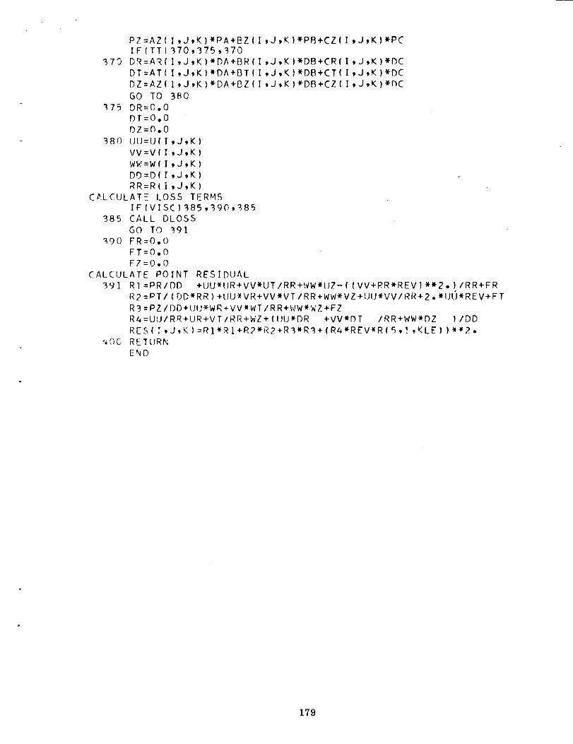
379
"475
38O
PZ=AZ(IF(TT)
DR=ARC
DT=AT(
DZ=AZ(
GO TO
DR=O.O
DT=O.ODZ=O.O
(JtJ=UI!
VV=Vll
WW=W(I
DD:D(I
I,J,K)*PA+BZ(I,J,K)WPB+CZII,J,K)wPC370,375,37'3
I,J_K)_DA+BR(I,J,K)_DB+CR(I,J_K)_DC
I,J,K)*DA+BT(I,J,K)WDB+CT(I,J,K)WDC
I,J,K)WDA+BZ(I,J,K)_DB+CZ(ItJ,K)_bC
38O
,J,K)
,J_K)
_J_K)
9J,K)
RR=R(i,J,K)
CD.LCULAT£ LOSS TERMS
IF(VISC)385,390,B85
385 CALL DLOSS
GO TO _gl
390 FR=O.O
FT=OoO
FZ=O,O
CALCULATE POINT RESIDUAL
3')1 RI=PR/DD +tJU*IJR+VVWUT/RR+WW_lJZ-( (VV+RR*REVI**2,)/RR+FR
R2 =PT/(DD*RR) +UU.W VR+VV*VT/RR+WW*VZ+UU*VV/RR+2, wUIJ*REV+FT
R3=PZ/DD+UU_WR*VV_WT /RR+NW_WZ +FZR4=UtJ/RR+UR+VT/RR+WZ+(IIU_DR +VV_DT /RR+WW_DZ )/DD
RES([,J,K}=RI_RI+R2_R2+R3WR3+(R4_REV*RI5,I,KLEI)_2o
_C)O RETURN
END
179
SUBROUTINE STAR
CALCULATION OF LOCAL STAR
COMMON1 D(IO,
2 DELXI3 AZ(IO4 CT(IO
5 IRSTA
RSTAR =
IGO=O
I=II
J=JJ
K=KKNBD=I
389 GO TOI375,378),IRSTAR
378 CALL RESID
375 RSTAR:RSTAR+RESII,J,K}
NRD=C
403 IGO=IGO+1GO TO (391,392,393,394,395,396,402)'IG0
391 I=II-1IF(I-1)400,_89,389
392 I=11+1
IF( [-IMAX)389,389,400
393 I=II
RESIDUAL
UIIO,IO,22},V(IO,IO,22),W(IO,IO,22)'P(IO*IO'22}'
IO,22),R(IO,IO,22),TIIO,]O,22),ZIIO,lO,22),FR'FT'FZ'DMAX(4)'
4),NSEQ(4), RES(lO,IO,22},AR(IO,lO,22),AT(]O,IO'22)'
,IO,22),BR(IO,IO,22),BTIIO,IO,22),BZ(IO,IO,22),CR(In,ln,22),
,IO,22),CZ(IO,IO,22),XH,RSTAR,TT,PSAT,DLIQ,REV,A,M,NVAR,NT_,
R,DX,I,J,K,II,JJ,KK,IMAX,JMAX,K_!AX,VISC,NBD,KLF,KTE
0,9
J=JJ-1IF(J-I)400,389,389
194 J=JJ+l
IF(J-JMAX)380,389,400
395 J=JJK=KK-1IF(K-1)400,389,389
396 K=KK+IIF(K-KMAX)389,389,400
402 RETURN
END
180

SUBROUTICALCULATION OF
COMMONU{1 D(IO,IO,2 DELX(4) ,3 AZ(IO,IO4 CT(IO,IC
5 IRST,AR,D
PSP=PSAT-
IF(PSP)IO
101 C(I,J,K)
GO TO 103
102 D(!,J,K)
103 RETURN
END
NE STATE
POINT DENSITY
]0,10,22},V(lO,IO,22},W(IO,IO,22),P(]O,lO,22),
22),R(IO,IO,22),TI10,IO,22),Z(IO,IO,22),FR,FT,FZ,DMAX(4),
NSEQ(4), RES(10,lO,22),AR(lO,IO,22),AT(]O,]0,22),
,22),BR(IO,10,22),BT(IO,IO,22},BZ(10,10,22),CR(IO,IO,22},
,22),CZ(IO,IO,22),XH,RSTAR,TT,PSAT,DLIQ,REV,A,M,NVAR,NTR,
X,I,J,K,II,JJ,KK,IMAX,JMAX,KMAX,VISC,NBD,KLE,KTE
P(I,J,K)
1,101,102
= DLIQ
: DLIQI( I,+TT_-PSP }
181

C DATA REDUCTION PROGRAM FOR RESULTS OF EXACT
C THREE-DIMENSIONAL INDUCER ANALYSIS PROGRAM
C - "
C TRW ACCESSORIES DIVISION, CLEVELAND
C
6AUG65
DIMENSION TITLE(16)COMMON U(IO,IO,22),VIIO'10'22) 'w(10'10'22)'m110'lO'22)'O(In'lq'22)
1 ,RIIO,IO,22),TIIO,IO,22),ZIIO,IO,22),AI10,IO,22)'QI]O'IO'22)'
2 UBI10,22),VB(lO,22},WBIlO,22),PB(10,22)'DBIlO'22)'RB(]O'22)'
3 DELP(IO,22),X(]O,10),Y(10,10),REV,DLIQ,PSAT,TT,IGO'I,J'K'IMAX'
4 JMAX,KMAX,IM1,JMI,B,SUB,TOT,OTOT
READ IOO],IMAX,JMAX,KMAX,KLE,KTE
READ IO03,(((R(I'J'K)'I:I 'IMAX)'J:I'JMAX)'K=I'KMAX)
READ IO03,(((TII,J,K),I:I,IMAX),J:I,JMA_),K:I,KMAX)
READ IO03,(((Z(I,J,K),I=I,IMAX),J:I,JMAX),K=],KMAX)
999 READ IOOC',TITLE
PRINT IO00,TITLE
READ IO0],KOUNTPRINT 1CI2,KOLINT
RFAD IO02,_LANKREAD IOC2,RFV,DLIO,PSAT,TT
READ IO02,(((I.;(I,J,K),I=],fMAX),J:I,JMAX),K=1,KMAX_
READ IO02,(((V[I,J, KI,I=I'IMAXI'-J=I'JMA×)'K=]'KMAX}
READ IO02,(((W(I,J'K)'I=I'I MAX)''J=I'JMA×i'K=!'KtzAX)RFAD IO02_(((P(I'J'K)'I=I'IMAX) 'J:I'JMAXI'<=!'KMA_)
CONVERT FROM ABSOLUTE TO RELATIVE VELOCITIFS AN_
CALCULATF POINT DENSITIFSDO ] K=I,KMAX
DO I J=I,JMAX
DO 1 I:I,IMAXV(I,J,KI:R(I,J,K)*REV+V(I,J,K)
IFCTT}2,3,2
2 PSP=PSAT-P(I'J'K)IF(PSP)3,3,21
21 D(I,J,K)=DLIQ/(I" +TT*pSP)
GO TO 1
3 D(I,J,K)=DLIO
I CONTINUE
CALCULATE INCREMENTAL THROUGHFLOW AREAS AND MASS FLOW RATES
I_I=IMAX-I
J_]=JMAX-I
DO 4 K:I,KMAX
DO 4 I=I,IMI
RBII,K)=(R(I,I,K)+RII4],],K))/2-
DO 4 J=I,JMIAII,J,K)=RB(I,K)*(R(I+I,I,K)-R(I,I,K))*(T(I*I'J+I'K)+T(I'J+]'K)
1 -T(I+I,J,K)-T(I,J,K})/2,
4 Q(I,J,K)=A(I,J,K)*(W(I,J,K}+W(I,J*I,KI+W(I+],J,K)+W(I+],J+],K)_W
1 (1)(!'J'K) +_)(I'J+I'K)+D(I+I'J'K_+_(!+I'J+]'<)_/IA"
CALCULATE AREA-AVERAGED O'J&NTITIES
DO 6 IGO:I,5
DO 6 K=],KMAX
DO 5 J:I,JMAX
DO 5 I=I,IMAX
GO TO (51,52,5_,54,55),IG0
5] XiI,J)=tJ(I,J,K)
GO TO 5
52 X(I,J):V(I,J,K)
GO TO 5
53 XII,J)=W(I'J' K)
182

54
555
61
62
63
64
656
GO TO 5X(I,J)=P(I,J,K)GO TO 5X( I ,J) =D( I ,J,K)
Y(I,J)=A(I,J,K)
DO 6 I=I,IMI
CALL SUM
GO TO (61,62_6_.,64,65),IG0
UB ( I ,K )=SUB/TOT
GO TO 6
VB( I ,K )=SUB/TOT
GO TO 6
WB ( I ,K )=SIJR/TOT
GO TO 6
PB( I,K)=._UB/TOT
GO TO 6
DB( I,K)=SUB/TOT
CONT INUE
CALCULATE MASS FLOW RATE PER CHANNEL
QTOT=O, 0
DO 7 I:1,I_41
DO 7 J=I,JM1
7 QTOT=QTOT+Q(I,J,])
CALCULATE MASS-AVFRAGED QIJANTIT!ES
K=KLE80 DO 8 IGO=1,3
CALL MAVGO TO (81,82,83),IG0
81 PF)=BGO TO 8
82 V2=B
GO TO 8
83 tJV:B
8 CONTINLJF
IF(K-I )l0,9, ] ,3
9 PDIN=PD
V21N=V2/2.
UV I N=UVK=KTE
GO TO 80IO PDEX=PD
V2FX=V2/2,
UVEX=UVDH=PDEX+V2E X-PD I N-V2 I NPSH= (UVEX-UV I N )*QTOT
EFF=DH*QTOT/PSH
CALCULATE BLADE-TO-BLADE PRESSURE LOADING
DO 12 K=] ,KMAX
DO 12 I=I,IMAX12 DELP(I 9K)=P(I,] I,K)-P(I,JNAX,K)
C *** OU'PUT ROUT I IXlE **_
PRINT 1004
DO II K=I,KMAX
IF(K-KLE} 11].]12,113
112 PRINT 1005
GO TO III
I13 IF(K-KTE)II],]]4,1]I
114 PRINT 1006
III PRINT I007, Z(l _I,K),RB(],K),UB(I.K),VB(I,K),WB(],K).PB(I.K},
] DR(I,K)
188

C
ii PRINT I00IPRINT 101DO i_i K=IF(K-KLE)
132 PRINT I00GO TO I_I
133 IF(K-KTEI134 PRINT131 PRINT
PRINTGO TO
1000 FORMA100] FORMA1002 FORMA1003 FORMA1004 FORMA
ISIIIl 9X
2 8X
1005 FORMA
]006 FORMA
IO07 FORMA
1008
1009
I010
1011
I012
8,(RB(I,K),UB(I,K),VB(I,K),WB(I,K},PB(I,K),DB(I,K),
I=2,1M]}
0
1 ,KMAX
131 ,I_2,1_3
5
131,1_4,!3l
1006
IOll,Z(1,1,K),(DELP(I,K),I=I,IMAX}1009, PDIN,PDEX_V2INgV2EX,DH,PSH,EFF,QTOT
999
INPUT-OUTPUT FORMATS ***
T(16AS)
T(2613)
T(BFIO.7)
T(IP6EI3.7)
T(I/IOX52HHUB-TO-TIP DISTRIBUTOINS OF AREA-AVERAGED OUANTITIF
IOXSHAXIAL,2(gx6HRADIAL),SX]OHTt_NGENTIAL,IOXSHAXI_I-,
6HSTATIC/2(8x7HSTATION),3(TXSHVELOCITY),7X8HPRFS£URE,
7HDENSITY//)
T(IXI8HBLADE LEADING EDGE)
T(IXIgHBLADE TRAILING EDGE}
T(/7F15.5)
FORMAT (15X6FI5 • =,)
FORMAT (III20X2aHMASS-AVERAGFD QUANT IT IES//2 (IOX5HINLET, 11X4_E× IT ) ,
I IOXSHTOTAL ,8XTHCHANNEL, 8 X 7HOvERALL 'SXTHCHAKNEI-/2 (7× 8HPRF c''£_jRE) '
2 2(TX8HVELOCITY),IIX4HHEAD,IOX5}ISHAFT,5XIOHEFFICIENCY'S IOX5HPOWER,26X4HRATE//SFI5.53 6X9HMASS-FLOw/4( IIX4HHEAD} ,IIX4HRI. E_
FORMAT(//2X9HZ-STATION,OX58HH_J-3-TO-TIP DISTRIBL,'T[ON 0 _ BLA!)F-TO-.nl
lADE PRESSURF LOADING//}FORMAT( FIl.4,9XIPlOE]0.4)
FORMAT(/23HRFDt._CED OUTPUT OF CYCLE,I'_)
END
184

SIlBROU
CALCULATE WE
COMNON1 _R(IO
2 UB(IO
3 DELP (
4 JMAX
SLJB=O °
TOT=O.
DO 1 J
SUB=SU
I TOT=TO
RFTURN
FND
TINE SU_
IGHTFD SUM
U(IO,10,22),V(10,IC,22),W(10,10,22),P(IO,IO,22)_D(IO,IO,22)
_IO,22),T(IC,,10,22),Z(IC,10_22)_A(Ie,10,22),O(IO*10,22),
,22},VB(IO,22)_WB(IO,22),PB(1O,22),_BI10,22),RB(]O_22)*
IO,22)_X(]O_10),Y(10,IO)_REV_DLIQtPSAT,TT,IGO,I,J_KtIMAX*
KMAX, IM ] ,JM ] ,B, SIJB,TOT _QTOT
O
0
=1,JM]B+Y(I,J)W(X(I,J)+X(I,J+I)+X(I+],J)+X(I+I,J+] ))/4,
T+Y(I,J)
185

SUBROUTINEMAVCALCULATEMASS-AVERAGES
2
3
I0
20
COMMON LI( I0,10,22 ) _V(10,I0,22 ),W( iO,I0,22 ) ,P (IO,10,22) 'D( 10' IO'22)
1 ,R (I0,10,22) ,T (10,I0,22 },Z(I0,IC),22) ,A (Ir_,19,22 ),Q( IC),1q,22 } _
2 UB(10,22),VB(lO,22),WB(lO,22),PB(]01,22),DB(]h*22)'RP'(]O'22) '
3 DELP(10,22 } 'X (] 0' 10) 'Y(10'10) 'REV*DL IQ' pSAT ' TT' IGO' I ' J'K' IF'_Ax '
4 ,KMAX, IMI ,JMI ,R ,SLJB,TOT ,QTOTJMAX
DO I0 J=I,J_IAX
DO 10 I=I ,
GO TO (I,2
X( I,JI=P( I
GO TO IO
X ( I ,J} =U( I
GO TO IO
X( I ,J) =R( I
Y( I ,J)=Q( I
B=O,O
DO 20 I=l ,
CALL SUM
R=B+SUBB=B/QTOT
RETURNEND
INAX
,3),IGO
,J,K)/D(I,J,K)
,J,K }*w2+V( I ,J,K }*w2+W( I ,J,K)**2
,J,K)_REV_V(t,J,K)
,J,K)
IM1
186
APPENDIX D
INSTRUCTIONS FOR USE OF APPROXIMATE
SOLUTION COMPUTER PROGRAM
This appendix describes the aPproximate analysis program including its two subroutines.
The latter one of these finds blade coordinates for any full blades having radial ele-
ments, constant thickness with or without radial taper and leading edge faring, and a
quadratically-varying lead. Any other shape would require a new blade coordinate
subroutine. The inputs and outputs are described, and block diagrams are included
with a complete Fortran IV listing.
1. Computer Running Information
The main program and its two subroutines have a common storage require-
ment of 13,513 locations. The maximum field capability is 11 streamlines
including hub and shroud, and 21 stations including blade leading and trailing
edges; i.e. an 11 x21field. The minimum isa2 x2 field.
Computer running time depends on the size of the field and the accuracy
required. The following estimates roughly summarize our experience on
computer times:
a) Time a No. stations
b) Time a (No. streamlines) 4
c) Time a .3/ 1 '_
V llowable unbalance
d) Time at stations where two-phase flow exists is double that for incom-
pressible flow.
For example, an 8 x 16 field with incompressible flow and an allowable
unbalance of. 001 took about 400 seconds on a UNIVAC 1107, while a . 01
unbalance took 185 seconds. A similar 4 x 6 field at . 001 balance took
24 seconds.
2. Input Data
The inputs to the program consist of (a) the title and program control
numbers; (b) the geometrical data for locating quasi-normal stations and
the streamlines at the blade leading edge; (c) the blade contour data;
(d) the speed, fluid properties and accuracy required; (e) the distributions
of fluid pressure, velocity and density at inlet; and (f) the various sets of
187

fluid data v, Psat and T* for which solutions with the foregoing inputs aredesired. Note that for splitter blades a separate problem should be solved
up to the splitter point, and the output should be used with a change in thenumber of blades nb to solve a new problem downstream of that point.
Following is a definition of each program input in the order required by the computer;
(the format is given in the Fortran listing):
TITLE: Any identifying information consuming up to 80 spaces.
NQI, NQJ:
MNC:
The number of streamlines (i or 1) and one more than the number
of stations (j or J) respectively. The extra station J = NQJ is
required for blade angle data at station J = NQJ-1. I = 1 on the
hub, and I = NQI on the shroud; J = 1 on the blade leading edge
and J = NQJ-1 on the blade trailing edge. The "field" stated
in table III. I quotes NQI x (NQJ-1), = qi x qj
The maximum allowable number of hub-to-shroud iteration cycles
at any one station. This Iimits the running time if the maximum
allowable streamline unbalance error EN (see below) is too small.
In such a case the computing continues and the resulting maxi-
mum unbalance is printed out. We used MNC = 25 in our 4 x 16
runs, (see results in table III. 1), and 1000 for 8 x 16. The actualnumber of cycles NC is dependent on EN and was usually 1/4
to 1/2 of MNC except in two-phase cases.
NDATA: The output data control number, specified as 0, 1, or 2. Theuse of NDATA is described in the output description further on.
This number makes it possible to omit all field data between the
inlet and outlet, thus saving considerable computing time when
several runs with small fields (say 4 x 16) are required simply
to establish overall performance at various combinations of
Rm, NPSH, and T*. With a 4 x 16 field, up to half the runningtime is consumed in the format and printing activity of the
computer.
NDB: A control number that is normally equal to zero. If NDB = 1,
a cycle-by-cycle account of the reduction of the total unbalance
tPf 2;.Ui, j) isprintedouttogetherwiththeattendantst ream-go 1 line adjustment magnitudes Sn' for stations
2 < J < NQJ-1. Following are the geometrical inputs:
z(I, i): The inlet axial positions _i of strealines at J -- 1 from hub to tip.
1 <--I---< NQI.
R(I, 1): The radial positions riatJ = 1. 1 < I< NQI.
188

Z(1, J):
R(1, J):
Z (NQI, J)and
R(NQI, J):
The axial positions of the stations j along the hub; i. e., the
locations of the hub-ends of the quasi-normals.
I= 1 and 2 < J < NQJ.
The radial positions of the stations along the hub. I = 1 and
2 5_ J <_-NQJ.
The axial and radial positions respectively along the shroud.
I=NQIand2 < J 5_ NQJ.
At this point, the following data is required by the blade subroutine:
AA, BB,
CC:
DSEX:
The lead constants a, b, and c respectively, which described
the radial-element pressure side of the blade according to theformula
d@- a + b_ + e_2
d_
The exit boundary layer displacement thickness _ ex , which
is assumed to exist on each side of the blade. The program
distributes _* linearly by station from zero at inlet, adding it
to the blade thickness.
T1T: The blade thickness t at the radial location R1T-- usually at
the inlet tip.
DTR: The radial blade taper constant where the blade thickness through-
out the machine (except in the fared region) is a function of radius
only and is given by
dt I (RIT) _r ]t = (TIT) + d--_-
We used no taper in our tuns.
ANB: The number of blades nb
TF(I, 2,3): The blade suction-side fairingconstants at stations 1, 2, and 3. The
blade thickness t at these stations is given by the product of TF and
the t of equation (A. 2). 0 <_ TF <- 1, and all material is removed
from the suction side only. We used TF(1) = 0 and TF(2 and 3) = 1.
Continuing now with the remaining inputs to the main program, wehave the fluid data:
(D. 1)
(D. 2)
189
EN:
RHOF:
OMEGA:
GO:
RHO (I, 1):
P(I, 1):
VM1 (I):
DELTAE(D:
VTB(I, 1):
V"
PSAT:
T:
PfThe maximum allowable streamline unbalance -- Umax.
goAs noted earlier, this value is exceeded if a balance cannot be
achieved in MNC cycles at any station J.
The liquid density Pf
The rotative speed f_, radians per unit time.
Constant in Newton's second law, go
The fluid density P i' in the middle of each annulus i or I at theblade leading edge where J = 1. 1 <-- I <-- NQI-1, since the number
of annuli is one less than the number of streamlines.
The fluid static pressure Pi' in each annulus. J -- 1 and
1 < I < NQI-1.
The velocity component in each annulus normal to the blade
leading edge at that point in the meridional plane.
1 <_ I < NQI-1.
The exit deviation angle $ex, i' of the relative flow from thedirection of the blade in each annulus. This deviation is distri-
buted from zero at inlet according to the sixth power of the
number of stations (_.m6), thus approximating an unloading
condition near the outlet. We used _ex = 0 for all our runs.
The tangential absolute velocity component V0, i' at the inletof each annulus. J: land 1 <_ I <__ NQI-1.
The fluid kinematic viscosity
The liquid saturation of vapor pressure Psat
The fluid thermodynamic constant T*
As many combinations of these three final inputs V, PSAT and
T may be added to the other data as the number of solutions
desired for unchanged values of all other inputs. For example,
NPSH depends on the difference between P(I, 1) and PSAT,
whereby a reduction of PSAT with constant values of say zero
for P(I, 1) increases the NPSH.
190

3. Output Data
All output data is printed in groups. Each is here defined together with the value of
the input control number NDATA for which that group can be obtained -- in the order
of their appearance and under the following headings:
a) Input data except for V, PSAT, T.
NDATA = 0, 1, or 2. No headings.
The following data groups are printed at station J = 1:
b) Streamline and blade data at station J.
e)
NDATA = 2:
I:
J:
R:
Z:
N:
TS:
TP:
Average fluid data at station J.
NDATA= 0, 1, or 2. Columns for annuliI-- 1,2,3,
I." The annulus identifying number i.
J: The station identifying number j.
RAV: The annulus mean radial position ri' .
ZAV: The annulus mean axial position _i'.
Printed in columns headed as follows for streamlines
I= 1, 2, 3 ..., NQI:
The streamline identifying number i.
The station identifying number j.
The streamline radial position r i.
The streamline axial position _i.
The streamline position n' i corresponding to r and _;
viz., the approximate meridional arc distance along
the blade leading edge from the hub.
The circumferential position Os, i of the suction surface
of the channel at location n' -- outside the boundary layer
displacement thickness.
The same for the pressure surface
..., NQI-I:
191

P: The static pressure Pi'.
W: The relative velocity Wi'.
VM: The componentof velocity Vm, i _in the meridionalstreamline direction, except at the leading edge (J = 1)
where this quantity is the input value VM1 normal to
the blade leading edge.
.!
VR: The radial velocity component Vr, 1 •
VZ: The axial velocity component V_, i.
D: The density P i'.
d) The first or next set of the final inputs V, PSAT, T ( v, Psat, T*) now
appears for NDATA = 0, 1, or 2 under the following heading:
KIN VISCOSITY, VAPOR PRESS,
VAPORZN CONST. -- THESE INPUTS USED
FOR THE FOLLOWING DATA.
The following output sequence is repeated for 2 < J <__NQJ-1; i. e., through
the blade trailing edge station.
e) Only if NDB = 1, the special cycle iteration data discussed under input
appears for NDATA = 0, 1 or 2.
f) Same as output (b) with the following additions: (NDATA = 2)
PfU i .
U: The resulting streamline unbalance go
NC: The total number of cycles executed at this station.
g) Blade-to-blade fluid data between stations J and J -1. (i. e., at station j')
NDATA = 1 or 2. Columns for annuli I = 1, 2, 3, .... NQI-1 with two
rows of data for each annulus. The first row gives I, J, RAV, and ZAV
as in input (c), and the following:
dWDWDT" The constant slope _ of the blade-to-blade relative
velocity distribution.
P: The mid-passage static pressure p i'"
.,PP: The channel pressure-side static pressure pp, 1 •
192
w
W: The mid-passage (mean} relative velocity Wi'.
WP: The pressure-side relative velocity Wp, i'.
D: The average density _i v.
,IDP: The pressure-side density Pp, 1
The second row repeats NC and U from output (f).
Also it gives the corresponding channel suction-
side data PS, WS, and DS.
h) Same as output (c). NDATA = 2, except at trailing edge (J = NQJ-1)
where this information is printed for NDATA = 0, 1, or 2.
The following additional data is printed for NDATA = 0, 1, or 2
after reaching the trailing edge:
i} Blade element data at exit.
Columns for annuli I = 1, 2, 3, ..., NQI-1.
•, calculated by equation (III. 22).LOSS COEFF: w 1
EFFICIENCY. _ i' calculated by equation (III. 23).
DEVIAT, ANGLE: 8ex, i' given by input DELTAE (I).
j) Overall performance data.
Listed in the following order, each having an appropriate heading:
n
AH
#2
V12/2g o
V2 2/2g o
w T
T*
calculated by equation (HI. 25)
calculated by equation (HI. 26)
calculated by equation (III. 26)
calculated by equation (HI. 27)
calculated by equation (HI. 27)
calculated by equation (HI. 24)
calculated by equation (HI. 28)
193

Pscalculated by equation (HI. 29)
calculated by equation (HI. 30)
, Psat and T* given by input, as is the value of after the next two items.
UNBAL ALLOW: _-o Um desired. This is the value of EN used at
input. The program stores it unchanged under the name
CRN.
MAX UNBAL ERR: Uma x obtained. This is the resulting value of
EN, which is the same as CRN if NC < MNC throughout
the calculations.
For each additional set of v, Psat and T*, a further set of outputs is printed,
beginning with (e) and continuing through (j). For any set that gives no
complete solution due to choking at low NPSH, the message "NPSH too low
for two-phase solution if NC less than MNC" is printed at the point where
this occurs, and the computer passes on to the next set. It is safe to say
that for typical MNC, even NC = MNC means no solution is possible at larger
numbers of streamline balancing iteration cycles NC. The computer will stop
with an input tape end-of-file condition.
194
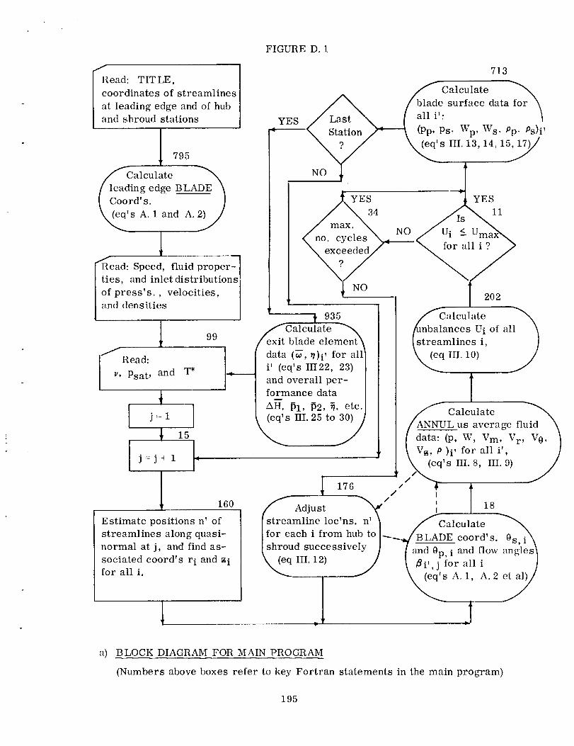
FIGURE D. 1
f
Read: TITLE,
coordinates of streamlines
at leading edge and of huband shroud stations
I 795
aleulate
ng edge _BL__ADE
d's. ]
_'s A. land A._//
1/
Read: Speed, fluid proper-
ties, and inlet distributions
of press's., velocities,
and densities
YES
713
Calculate
data for \surface
Ps, Wp, Ws, pp. Ps)i'
's III. 13, 14, 15_,/
YES YES
34 11
max,NO U i !
no. cyclesexceeded for all i ?
NO
99
/Read:
_, Psat, and T* .___
1j=l [
15
j=j+l [-"
l 160
Estimate positions n' of
streamlines along quasi-
normal at j, and find as-
sociated eoord's r i and z ifor all i.
t 935
e_xitCalculate -_
blade elementdata (_, _)i' for all'
i' (eq's III22, 23)
and overall per-formance data
AH, Pl, _2, _, etc.
(eq's III. 25 to30) j
1/
202
176 / 4 4] 1
18/
[streamline loc'ns, n' / / CalculateI for each i from hub to I-__..JBLADE coord's 0o _\
shroud successively _ " S, 1[shro_ ly ] 7a_, i and flow 2S_les_
(eq III. 12) / / Bi', j" for all i
"_" _] _ _s A.I,j A. 2 e_/
',aleulate
s U i of al
streamlines i,
(eq IH. 10)
IA_NNU Calculate
L us average fluid \_W' Vm' Vr' V0' I
V_, 0 )i' for all i', ]
/_'snI. 8, III. 9) /
a) BLOCK DIAGRAM FOR MAIN PROGRAM
(Numbers above boxes refer to key Fortran statements in the main program)
195

FIGURE D. 1 (Continued)
ubroutine ANNUL
5O
AssumeNew Two-Phase
Oi',j
Assume liquid
._-----__ flow, i.e._*'1 ,j Pf
/_aleulate Annulus_
/ Outiet Velocity Diagram'_
I c_' Vm, vo) i', j ]
_s. III. 8, etal)/
C,alculate Annulus_
tlet Pressure,
j (eq III. 9) /
16 et al
to_C_lleulate Blade-_
ade W and
I Distributions
sHI. 14 et al)
_YES
_k,_OL=U J- /Z_alculate _'_
W i.
NO 41 38
_i C°ntinuity _k //_aleulate Blade_
?/'Pi, j+ Pi, j-l_\ [ to-Blade Average
', J= \ 2 --] _*_--_ De? si,ty
Test / _] (eqlII 19)J
b)
YES
4O
BLOCK DIAGRAM FOR SUBROUTINE "ANNUL"
/ Two- Phase_
I"°
(Numbers above boxes refer to key Fortran statements in the subroutine)
196

FIGURED. 1 (Concluded)
JfRead: Blade lead con-
stants a, b, c; Blade andboundary layer thicknessdata andnumber of blades
SubroutineBLADE
(1st time only) 24
_slCUlate ]_
age hydraulic
eters Dh, j for
1_ 6, 5, 8,10 or 11
_Calculate )
1
gle 0p of pressure
e of channel
. A. 1)
/blade thickness t \
I (eq. A. 2) including}
\boundary layer thickness/
c)
f Calculate e_gle 0 s of suction sid
channel
BLOCK DIAGRAM FOR SUBROUTINE "BLADE"
(Nqmbers above boxes refer to key Fortran statement numbers in the subroutine)197

C
C
C
C
TABLE D. I
FORTRAN IV LISTING OF APPROXIMATE ANALYSIS PROGRAM
APPROXIMATE 3-DIML INDUCER ANALYSIS FOR NASA AUGUST20, 1965
TRW ACCESSORIES DIVISION, CLEVELAND, OHIO
DIMENSION Z(ll,22),R(]I,22),AN(ll,22),TP(]1,22),TS(1],22),RHO(IO'
121),RB(IO,22},ZB(IO,22},TPA(IO)tTSA(10),TA(IO),SRFA(lO),SBF(IO)'
2CBF(10),DT2(IC),FLC(10},RVT(10),DEM(]O),P(1O,21),VTR(]O,21),WB(]9'
321),DELDB(11,22),AK(10,21),LJ(ll,2]),ACOSGJ(22),SJ(22),W(1h}'DELTAE
4(IO),B(10),VMI(IY)tVM2(IO),VII]O),AM](IO),VR](]C),VZ](IO),VR(]O)'
5VZ(10},ALOSS(10),DHP(22),ANN(]O),CONV(Ie}
COMMON AN,RR,ZZ,R,Z,Fpp,TSS,PBI,PB2,WBI,_f32,RHOBI,RHOB2,RHOF'PSAT'
IGO,ANB,PIE,AK2,T,DHP,J,NOI,NQJ,V,FC,FR,FSA,S_F2'CBF2'T_P'T_S'TDq'
2RB2 ,RVT 1 , ISTART ,AW,VBT2,0MFGA ,AC2 ,VBM2 ,CNV
1000 FORMAT (8CH
1 )
1001 FORMAT(]615)
1002 FORMAT(BFIC.4}
10C3 FORMAT(//2X,,_SHSTREAMLINE AND BLADE DATA AT STATION
I 4X, IHJ,7X, IHR, lqX, IFZ ,IkX, IHN, 14X,2HTS, 13X, 2HTP/
IU04 FORMAT(//2X,38HSTREAMLINE AND BI_A{)E DATA AT STATION
1 4X, IHJ,7X, IHR, 14X, IHZ, 14X, ]HN, ]4X'2HTS' 13X' 2HTP'
22HNCI (2 I5, lPSEI 5.7,,.i I8 ) }
1005 FORMAT(//2X,_IHAVF_RAGE FLIJID DATA AT '_TATION J/4W,I
I 6X,314RAV,qX,3HZAV, 9X, IHP, 1 ] X , ]H,.V,l 1X ,,2
2 2HVR, ]0X,PHVT, IOX,2HVZ, 10X, ].HD/ (215, IP�F ]2"4) )
1008 FORMAT(//2X,'_2HBLADE-TO-BLADE FLUID DATA i._ETWEEN £T
11 14X, I H I ,4 X , 1HJ, 6 X ,3HR AV, 9 X, 3147AV, 8 X ,Z_HDV,r)T, 9X , IHP,
21HW,IIX,2HWP'IC'X'IHD' IIX,2HDP/28X,2HNC'I[X'!Ii!#'22X'
322X ,2HDS }
1009
I010
1011
1012
1013
FORMAT (215 ,]P�FI 2 .a)
FORMAT (26X ,1 I5,3X , IPlEI2.4,12X , IPIFI2.4 ,]2X, !PlFI2.4,12X, ]P] F! 2.4 }
FORMAT(Y/2X,26H"SLADE ELEMENT DATA AT EXIT/aX,IH!,SX,If'HLOSS COEFF.,
]SX,]OHE.FICIF_NCY,'_X,]2HDEV!AT ANGLE/(] I5,1P3FlS.7) 1
FORMAT(///2X,,,24HOVFRALL PERFORMANCE DATA//3X,.12HTOT HEAl) CHG,_X,
111HPRESSURE IN,3X,12HPRESSURE CtJT,3X,,12HVEI_Y HE._D IN,?X,I"_HVELY HF
2AD OUT,1X,14HMASS FLOW RATF.,,,:)X,6HTORQIJE,4X,IIHSHA_--T POWFR/
31P8E15.7}FORMAT(//3X,12PIOVERALL EFFY,3X,12HANGI!LAR VFI_Y,4X,11t--ILIQ DFºNSITY,
14X,11HVAPOR PRESS,2X,13HVAPORZN CONST,4:,C,111.4[!NBAL ALLOW,2X,131.twh&×
2UNBAL ERR,3X,12HNO OF BLADES/IPSE15.7)
CONST,6X,4tH-fl4ESE INPUTS LISFD
FORMAT(//4X,liHJ,3X,SHCYCLE,4X,12HSTLN ADJ
FORMAT(II5,]IT,_X,IP2F]S.7)
FORMAT(//2X,71HNPSH TOO LOW cOR TWO-PHASE
I IF NC LESS THAN _NC}
PlE=_,]415')27
ISTART=I
READ ICO0
PRINT 1000READ IO0],NQI,NOJ,MNC,NDATA,KDB
PRINT ]O0],NQI,NOJ,MNC,NDATA,NDB
READ 1002'(7(I'])'I=]'NQI)
PRIN_ IOI5,(Z(I,]),I=I,NQI)
READ IOO2'(R(I'I)'I=I'N31}
PRINT 1015,(R(I,I},I:I,NQI)
REA_ 1002'(Z(I'I)'!=2'NQJ)
PRINT I015,(Z(I,I},I=2,NQJ)
READ IOO2,(R(I,I),I=2,NQJ}198
FORMAT(IP8FIS.7)
FORMAT(IIIII2X,13HKIN VI SCOS I TY,4X , 11HVAFOR PRESS,2X,FOR THF FOLLOW!f',IG ,")^T/_)
'1"MAG,4X,!]HTOT/_L .. ,IBAI..)
SCL['TION WITH THIS FLUID.
J/4X,]HI,
(215,1PSE]5.
J/4×,IHI,
13X,IHU,ICX,
7))
HI,4×,IH,J,
HVM,]qX,
AT IONS J AND J-
] I'_,21-PP, 19×..
2HPS, 22X, 2HW < ,
I015
1016
] ]3HVAPORZN
102U
1021
1022

7o5
1
PRINTREAD
READ
I015.[R(],I),I:2,NQJ)IOO2,iZINQI,I),I=2.N_J)
IOIS.(ZINQI,II,I=2.NQJI
IO02,(RINQI,I},I:2,NQJI
IOI5.(R(NQI,I).I=2,NQJI
SET UP FIELD OF HUB, SHROUD AND LFADING EDGE COORDINATES
AN(I,I):O,O
I=1
DO 795 J=I.NQJ
RR:R(I.J]
ZZ=Z(1.J)
CALL BLADE
TPII,J)=TPP
TS(I,JI=TSS
J=l
I=I+l
AN(I,1 )=AN(I-I,] )+SQRT(((7(I,!)-Z(I-!,] )}"w'*2o)+((P(I,])-R(I-I,I) )*
1"2.})
RR=R( I ,] )
ZZ=Z( I , ] l
CALL BLADE
TP(I 91)=TPP
TS ( I , I )=TSS
IF(NQI-I}7,7.1
7 J=J+l
AN(NQI,.J)=SORT(((R(NQI ,JI-R(],J) )*_2.)*((Z(NOl ,J)-Z(1,.J) }*'2.) )
ACOSGJ(J)=(R(NQI,J)-P.(I,J) )/AN[NQI.-J}
SJ[J)=(Z(NQI.J)-Z(I...J) )/AN{NQI,J)
5 IF (J-NO J)7,6,6
6 NO) I=NOI-]
ANQQ=NQ I I
REAl) 1002,EN,RHOF,Ot4EGA,GO
PRINT 1 ()I_ ,EN, RHC)F ,OMEGA ,GO
READ ].002' (RHO( ! , 1 } , I :] ,NO) I )
PRINT i015. (_l_O( I ,I) , I:l .NQI I )
READ ] (I(')2_• (P( I ,I ) .I=l ,NOT I )
PRINT IO15,(P(I,I) ,I=] ,NOI I)
READ IC)02. (V_'] ( I ) , I=l ,NQI I )
PRINT I0] 5, (VN11 ( I ) 9I=l ,NOI I )
READ IOfl2,(DELTAF(1),I=I,.NOI I)
PRINT I015 _ (OELTAE(I) , I=l ,NOI I )
REAr) ]r)o2,(VTB(_,I } ,:=].I'!C)!I )
PRINT 1015, (VTB( I ,I). I=] .NOr I )
DO 2 I=I,NQII
RB(I,I)=(R(I,I }+R(I+],1))/2.
B(I )=AN(I+I,I)-AN(I,I )
DELDB( I,I )=C),ZB(I,])=(Z(I,I )+Z[ I+I,1) }/2.
VRI(1)=VMI(1)*(Z(I,I,-Z(I+],!.))/B(1)
VZI(1)=VMI(Z)W(R( I+I,!)-R(I,!))/R(; ]
W( I )=VMI ( I )'2 .*P IF*RB( I ,1 )*B (_ __-RHO [ ! ;] 1
VI(II=VTP.(I,I}*VTF_(I,I)+VM] (1)*VN'I (1)
AM] (1)=RB( 1,1 )*VTR(I,] )
2 WB(I,I)=SQRT( I (OMEGA*RB(I,I }-VTP.(I,] ))**2.)+V v] ( I )*V_I (1))
J=1
I F(NDATA-I )45,45,44
44 PRINT IO03,(I,J.R(I,J),Z(I,J),AN[I,J).TS(I,J),TP(I,J).I=].NQI)
45 PRINT ]O05,(I,J.RIB(I,J),ZB(I,J),P(I.I),WB(I,I),V_!(1),
199
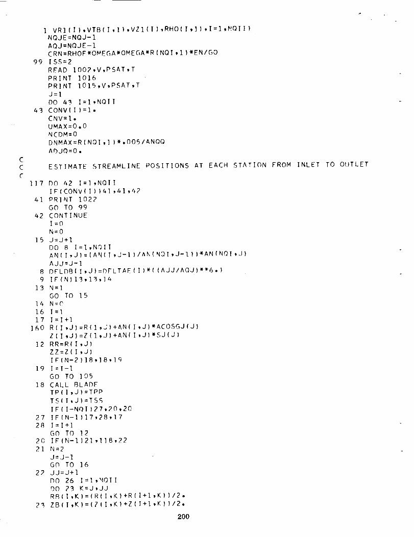
CC
C
99
4"3
VRI(1).VTB(I.I),VZI(I}.RHO(I,]).I=],NQII)
NQJE=NQJ-1
AQJ=NQJE-1
CRN=RHOFWOMEGA*OMEGAWR(NQI,I}*EN/GO
IO02.V.PSAT.T
I016
IOI5.V,PSAT,T
ISS=2
READ
J=l
DO 43 I=I.NQII
CONV(1)=I.
CNV=I.
UMAX=O,O
NCDM=O
DNMAX=R(NQI,I)W.OOS/ANQQ
ADJQ=O,
ESTIMATE STREAMLINE POSITIONS AT EACH STATION FROM
lI7 DO 42 I=I.NOII
IF(CONV(1))41,41,42
41 PRINT I022
GO TO 99
42 CONTINUEI=O
N=0
15 J=J+lDO 8 I=I.NOII
AN(I.J)=(AN(I.J-I)/AK(NgI,J-1))*AN(NQI'-J)
AJJ=J-I
8 DELDB(I,J)=_FLTAE(1)W((AJJ/AQJ)**6"}
9 IF(N)13,13,]_
13 N=IGO TO 15
14 N=O
16 I=1
17 I=I+l
160 R(I,J)=R(],j)4AN(I.J)*ACOSGJ(J}
Z(I,J}=Z(].,J)+AN(I,JIwSJ(J)
12 RR=R(I,J)
ZZ=Z(I,J)
IF(N-2)lS,]B,lG
19 I=I-1
GO TO 105
18 CALL BLADETP(19J)=TPP
TS(I_J)=TS£
IF(I-NQI)27_20,20
27 IF{N-1}17,28,17
28 I=I+l
GO TO 12
20 IFIN-1)21,118_22
21 N=2
J=J-1GO TO 16
22 JJ=J+1
DO 26 I=l,NOII
OO 23 K=J,JJRB(I.K)=(R(I.K)+R(I+I,K))/2.
23 ZB(I,K}=(Z(I,K)+Z(I+I,K))/2.
200
INLET TO OUTLET

C
24
25
26
104
100101
102
DDM=SQRTI(RBII,J)-RBII,J-III**2,+(ZRII,J)-ZBII,J-]))_2°)
DEMIIi=SQRTIIRBII,J+II-RB(I,J-III**2,+IZ_II,J+II-ZRII,J-II)W*2,)
DT2{I)=(TS(I,J)+TS(I+I,J)-TP(I,J)-TPII+I,J))/2,TBI=(TS(I_J-1)+TP(I,J-II+TS(I+],J-II+TP{I+I,J-])}/4,
TB2=(TS(I,JI+TPlI,J)+T£II+I,JI+TP(I+I,J))/4,
TB3=ITS(I,J+II+TP(I,J_II+TS(I+I,J+II+TPII+I,J+I))/4,
DT2(II=DT2(1)wSIN(ASIN(ABS((ZB(I,J÷I)-ZB(I,J-]})/DEM(1)))+ACOS(
]ARS(ACOSGJ(J)})}
RVT(1)=RB(I,J-I)*VTR(I,J-1}
BB2=ATAN(DEM(1)/((TB]-TB3)WRB(I,J}))
BF2=BB2-DELD_(I,J)
SBF(I)=SIN(BF2)
CBF(1)=COS(RF2)
BBB=ATAN(DDM/((TBI-TB2)_((RB(I,J)+RB(I,J-]))/2.)))
B_F=BBB-(DEL_(I,J)+DELDR(I_J-I))/2,£RFA(I)=SIN(_RF)/_DM
TPA(I}=(TP(I,J-1)+TP(I+]_J-1)+TP(I,J)+TP(I+],J})/4,TSA(I)=(TS(I,J-1)+TS(I+IgJ-1)+TS(I,J)+TS(I+l,J))/4,
TA(1)=(TPA(1)+rSA(1)I/2.
IF(V)24,24,25
CALCULATE FRICTION LOSS EFFICIENT
FLC(1)=O,
GO TO 26
FLC(1)=(.OOT16+.610_/((WB(I,J-l)*DHP(J)/V)**.35))/
] (2**DHP(J)WSBFA(1))
CONTINUE
I=O
I=I+1
RR(I,J}=(R(I,J)+R(I+],J))/2.
FR=(OMEGA_CMFC;A/?,}*(Rn(I,J)*RR(I,J)-RB(I,J-])WRR(I,J-I)}
AC2=RB(I,JI*_T2(I}WSORT((R(I+],JI-R(I,J)}*_
I 2.+(Z(I+I,J)-Z(I,J)}**2.)
FC=FLC(1)
FSA=SBFA(1)
SBF2=SBF(1)
CBF2=CBF(1)
TBP=TPA(I)
TRS=TSA(I)
TDB=TA(I)
RVT]=RVT(I}RB2=RB(I,J)
RHOBI=RHO(I,.J-1 )
PRI=P(I,J-I)
WRI=WR(I,J-I}
AW=W(1)
CALL ANNUL
RHO(I,J)=RHOB2
P(I,J)=PB2
WB(I_JI=WB2
VTB(I,J)=VRT2
VM2(I)=VBM2
AK(I,J)=AK2
CONV(1)=CNV
IF(N-3)IOC,IO],]02
IF(I-NOI+2}]O6,]O_,103
N=4
I=I+l
GO TO 105
N=3
GO TO I07
201

C
CC
C
C
C
C
C
103
178
NC=ODELLN=DNMAX
N=3
IJ(l,J)=O.O
U(NOI,J)=O.O
IF(NQI-2)]IB,118,202
I=lNADJ=O
CHECK ACCURACY OF STREAMLINE BALANCE FROM tIUB TO SHROUD
IF SATISFACTORY, PROCEED TO STATION OUTPUT CALCULATIONS
IF UNSATISFACTORY, PERFORt_ STREAMLINE ADJLJSTMENTS
113 I=I+1
IF(U(I,J)-CRN)IlI,]II,B4
l]] IF(I-NOII)II_,29,29
34 IF(MNC-NC)804,804,112
804 DO 50 I=2,NQII
IF(U(I,J}-UMAX}50,50,40
40 UMAX=U(I,J}
EN=EN*UBIAX/CRN
5O CONTINUE
29 N=I
I=2
GO TO 12
PFRFORM STREAMLINE ADJUSTMENT SEQUENCE
] ]2 NC=NC+I
I=]
172 I=I+l
VMHI=VM2( I-1}
VMH2=VM2(I }
CNVHI=CONV(I-])
CNVH2=CONV(1)
AKHI=AK ( I-I ,J }
RHOBHI:RHO(I-I ,J)
PBHI=P (I-] ,J)
WF_HI=WB(I-I,J)
VTBHI=VTB ( I-1 ,J )
LJH] =U( I-I ,J)
UH2=U( I ,J)
UH1=U( I+1 ,J}
AKH2=AK ( I ,J}
RHOBH2=RHO ( I ,J}
PBH2=P ( I ,J}
WBH2:WB(I,J)
VTBH2=VTB(I,J}
ANH=AN ( I ,J}
RHLD=R(I,J)
ZHLD=Z ( l ,J}USTAR=U(I-] ,J)WU_ 1-] ,J)+lJ{ I,J)*U(I,J)+U(I+I'J}*U{ I+],J)
176 AN(I,J)=ANH+F)FLLN
GO TO ]6O
750 USTARD= U(I-I,J)*U(I-I,J}+U(I,J}_WU(I,J)+Li(I+],J)*II(I+]'J)
IF (DELLN) 613,8C;8,5]0
STOP 808
IF (ADJQ }6] 2,6]2,611
ADJQ=O.
I F (IJSTARD-USTAR) 170,615,615
_.02
808
610
611

612
613
6135
614
169
615
6]6
6]7
30
31
618
619
62O
170
]80
152
32
174
173
33
175
177
35
179
USTARP=USTARDDELLN=-DELLN
GO TO ]76
USTARM=USTARD
DFLLN=ABS(DELLN)
UND2=(USTARP+USTARM-2.wUSTAR)/(DELLN_DFLLN)
IF(UND2) 615,6]5, 614
USND=IUSTARP-USTARM)/(2,*DELLN)
AN(I,J) = ANH-USND/UND2
ADJQ=I.
GO TO ]60
IF (USTARP-USTAR) 618,616,6)6
IF (USTARM-USTAR) 620,617,617
AN( I ,J )=ANH
IF(NCDM)30,_O,_I
DELLN=DELLNIIO. -_
NCDM=I
GO TO 176
DELLN=DELLN*]O.
GO TO 179
IF(USTARM-USTARP) 620,619,619
AN(I,J)= ANH+DELLN
GO TO 169
AN(I,J)=ANH-DELLK
GO TO 169
NADJ=I
NCDM=O
IFII-NOlII172,]73,]73
IF(NADJ)174,]74,]78
IF(DELLN-DNM_X/lOCC, o}178,]78,35IF(NDB-])32,?3,]75
PRINT ]O20
NDR=2
TOTAL=O,O
DO 177 KS=2,NCII
TOTAL=TOTAL+U(K8,J)
PRINT 102I,J,NC,DELLN,TOTAL
GO TO 32DELLN=DELLN/]0,
GO TO ]78
AK(I-I,J)=AKH]
VM2(I-])=VMH]V_2(I)=VMH2
CONV(I-])=CNVH]
CONV(I)=CNVH2
RHO(I-I,J)=RHOBH]
P(I-],J)=PBH]WB(I-1,J)=W_H1
VTR(I-],J)=VTBH]
U( I-] 9J)=UH]
U ( I ,J ) =UH2
tJ(I+I,J)=UH3AK(I,J)=AKH2
RHh(I,J)=RHO£H2
P(I,J)=PBH2
WR(I,J)=WBH2
VTB(I,J)=VTRH2
AN(I,J)=ANHR(I,J)=RHLD
ZII,JI=ZHLD
203
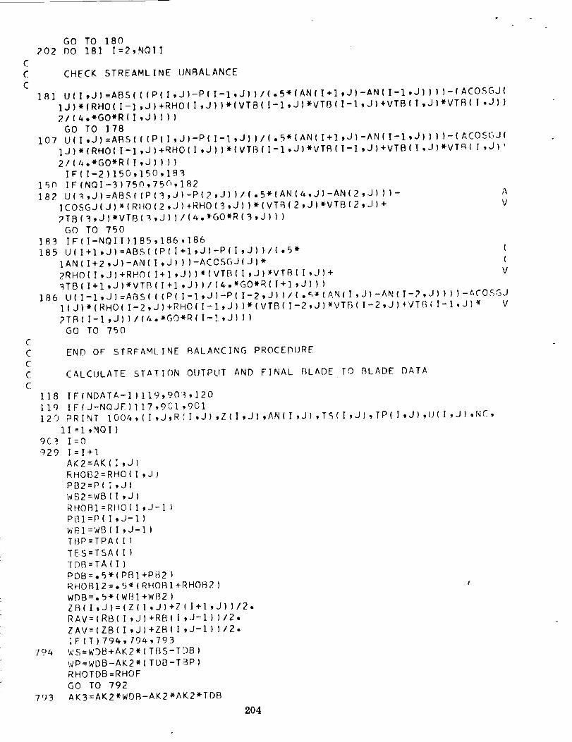
C
CCC
C
GO TO 180202 DO ]81 I=2,NOIT
CHECK STREAMLINE UNBALANCE
181 U(I,J)=ABS(((p(I,J)-P(I-1,J}}/(.5*(AN(I+I,J)-AN(I-1,J))})-(ACOSGJ(
Ij).(RHO(I-I,J)+RHO(I,J)}*(VTB(I-I,J)WVTB(I-I,J)+VTB(I,J)*VTR(I'J))
21(4.*GO*R(I,J))))
GO TO ]78107 U(I,J):ABS(((p(I,J)-P(I-1,J))/I.5*(AN(I+]tJ)-AN(I-1,J))})-(ACOSGJ(
]j).(RHO(I-I,J}+RHO(I,J)I_(VTB(I-I,J}WVTB(I-].,J)+VTB(I,J}WVTR(I'J)_
2/(4.*GO*R(I,J))))
IF(I-2)150,]50,IB3
150 IF(NQI-3)750,750,182
182 U(_,J)=ABS((P(_,J)-P(2,J))/(.5*(AN(A,J)-AN(2,J)))- A
]COSGJ(j)W(RHO(2,J)+RHOIS,J))W(VT_(2,J).VTB(2,J)+ V
2TB(3,J)*VTB(_,J))/(4.*GO*R(3,J}))
GO TO 750
183 IF(I-NQII)]B5,186,]86
185 U(I+I,J}=ABS(iP(I+I' J)-p(I'J))/('5* (
]AN(I+2,J)-AN(I,J)))-ACOSGJ(J)* (
2RHO(I,J)+RHO(I*.],J))*(VTB(I,J)_VTB(I'J)+ V
186
3TB(I+I,J)*VTB(I+],J))/(4.wGO*R(I+],J)))
U(I-1,JI=ABS(((P(I-1,J)-P(I-2,J))/I-_*(AN(I,JI-AN(I-2,JI}))-_CO_GJ
I(j).(RHO(I_2,J)+RHO(I-I,j))*(VTB(I-2,J)-WVTB(I-2,J)+VTB(I-I,J)W V
2TR(I-I,J))/(4.*GO*R(I-!,J)))
GO TO 75O
END OF STRFAMLINF BALANCING PROCEDURE
CALCULATE STATION OUTPLIT AND FINAL BLADE TO BLADE DATA
118
1!9
120
9C _.
929
7 _4
793
IF(NDATA-I)II9,903,120
IF(J-NQJE)II7,gCI,901
PRINT IO04,(I,J,R(I,J),Z(I,J),AN(I,JI,TS(I,J),TP(I,J),U(I,JI'NC'
II=I,NQI}
I=O
I=I+l
AK2=AK(:,J}
RHOB2=RHO(I,J}
PB2=P(I,J)
WB2=WB(I,J)
RHOBI=RI_O(I,J-I)
PBI=P(I,J-I}
WBI=WB(I,J-I)
TBP=TPA(I}
TBS=TSA(1)
TDB=TA(1)
PDB=.5*(PBI+PB2)
RHOB12=,SW(RHOBI+RHOB2) ¢
WDB=.5*(WB]+WB2)ZB(I,J)=(Z(I,J)+Z(I+I,J))/2.
RAV=(RB(I,J)+RB(I,J-I))/2.
ZAV={ZB(I,J)+ZB(I,J-I))/2.
IF(T)794,104,793
WS=WDB+AK2*(TBS-TD8)
Wp=WDB-AK2*(TDB-TBP)
RHOTDB=RHOF
00 TO 792
AK3=AK2*WDR-AK2*AK2*TDB
204
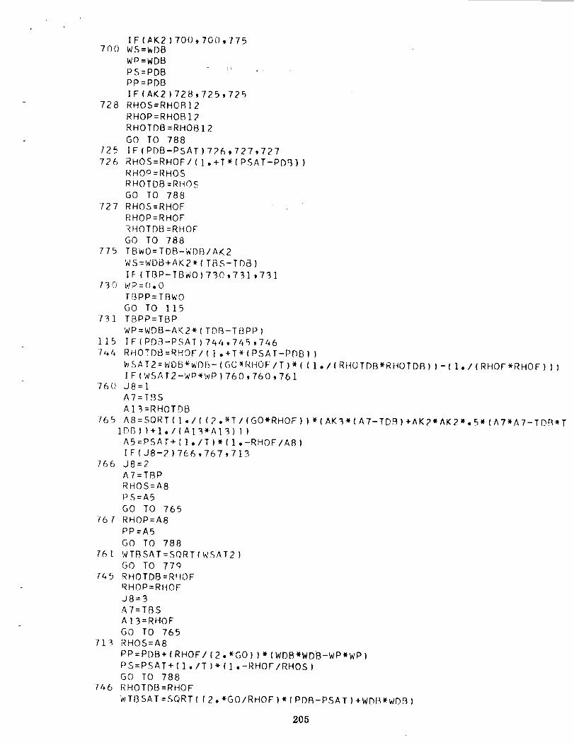
I F(#K2 } 700,700,775700 WS=WDB
WP=WDBPS=PDB _PP=PDB
IF(AK2)728,725,725
728 RHOS=RHORI2
RHOP=RHOB12
RHOTDB=RHOBI2
GO TO 788
125 IF(PDB-PSAT)726,727,727
726 RHOS=RHOF/{1.+T*(PSAT-PDB))
RHOP=RHOS
RHOTDB=RHOS
GO TO 788
727 RHOS=RHOF
RHOP=RHOF
RHOTDB=RHOF
GO TO 788
775 TBWO=TDB-WDB/AK2
WS=WDB+AK2W(TBS-TDB)
IF(TBP-TBWO)730,731,71]
WP=(;.O
TBPP=TBWO
GO TO 115
TBPP=TBP
WP=WDB-AK2*(TDB-TBPP)
IFIPD3-PSAT)744,765,746
730
731
115
1_+4 RHOTDB=RHOF/(lo+T_(PSAT-PDB))
WSAT2=WDB*WI)B-(GG*RHOF/T)*((I./(RHOTDB*RHOTDB))-(I./(RHOF*RHOF)))
IF(WSAT2-WP*WP)760,760,76176(; J8=l
A7=TBS
AI_=RHOTDB
765 AB=SQRT(I./((2.*T/(GO*RHOF))W(AK3W(A7-TDB)+AK2,AK2,._,(ATWA7_TDR,TIDB))+I./(AI_WAI3)))
AS=PSAF+{]./T)*(I.-RHOF/A8)
IF(J8-2)766,767,713766 J8=2
A7=TBP
RHOS=A8
PS=A5
GO TO 765
767 RHOP=AB
PP=A5
GO TO 788
761 WTBSAT=SQRT(WSAT2)
GO TO 77Q
745 RHOTDB=RIIOF
RHOP=RHOF
J8=3
A7=TBSA|3=RHOF
GO TO 765
713 RHOS=A8
PP=PDB+(RHOF/(2.*GO)}W(WDB*WDB-WP*WP)
PS=PSAT+(]./T)*(I.-RHOF/RHOS)
GC) TO 788746 RHOTDB=RHOF
WTI3SAT=SQRT((2.*GO/RHOF)*(PDR-PSAT)+W_B,WDB)
205
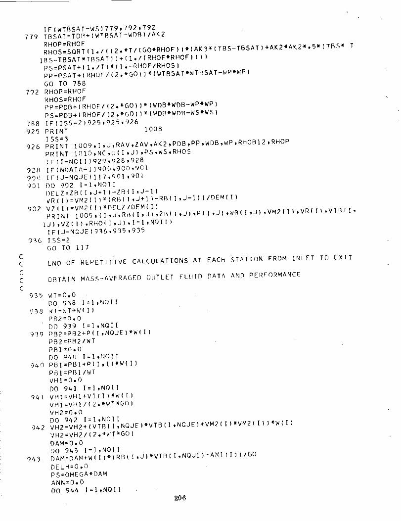
CC
C
C
C
IF(WTBSAT-WS)779,792'792
779 TBSAT=TDI_ +(WTBSAT-WDR)/AK2
RHOP=RHOFRHOS=SQRT(]./((2..T/(GO_RHOF)}.{AK3.(TBS_TBSAT)+AK2.AK2*.5*(TBS* T
IBS-TBSAT*TBSAT))+(I./(RHOF*RHOF)))}
pS=PSAT+II./T)_(].-RI_OF/RHOS)
pp=PSAT+(RHOF/(2.*GO))*(WTBSAT_WTBSA T-WP_WP)
GO TO 788
792 RHOP=RHOF
RHOS:RHOFpp:PDB+{RHOF/I2.*GOI}*IWDB*WDB -WP_WP)
pS=PDB+(RHOF/12,*GO)I*(WDB*WDB -WS*WS)
788 IF(IS5-2)925,925,926
925 PRINT 1008
ISS=3926 PRINT IO09,19J,RAV,ZAV,AK2,PDB,PP,WDB,WP'RHOBI2'RHOP
PRINT IOIO,NC,UII,J},PS,WS,RHOS
IF(I-NQII)929,928,928
928 IF{NDATA-I}900,900,901
900 IF(J-NQJE)IIT,QOI,901
901 DO 902 I=ItNQII
I)ELZ=ZBII,J+I)-ZBII,J-I}VR(I)=VM2IIi*(RBII,J+I)-RBII,J-1})IDEM{I)
902 VZII):VM2(I} _IbELZ/DEM(I)PRINT IO05,(I,J,RBII,J},ZB(I,JI,PII,J),WBII,J}'VM2II)'VR(I}'VIB{I'
IJi,VZ{I},RHO{I,J},I=I'NOII)
IFIJ-NOJE}gB6,935,g35
9B6 15S:2
GO TO 117
END OF REPETITIVE CALCULATIONS AT EACH
OBTAIN MASS-AVFRAGED OUTLET FLLIID DATA
STATION FROM INLET TO EXIT
AND PERFORMANCE
935 WT=O.O
DO 938 I=I,NOll
938 WT=WT+W(1)
PB2=O.O
DO 939 I=I,NQII
939 PB2:PB2+PII,NQJE}*WII}
PB2=PB2/WT
PBl=O,O
DO 940 I=I,NQII
940 PBI=PBI+P{I,I }*w(1)
PBI=PBI/WT
VHI=O.O
DO 941 I=],NQII
941VHI=VHI+V]{I )*WII)
VHI=VHI/I2.*WT*GO}
VH2=O.O
DO 942 I:I,NQII942 VH2=VH2+( VTBII'NOJE)*VTB(I'NCJE}+VM2(I)_VM2(I)}*WII}
VH2=VH2/{2.*WT*GO}
DAM=O.O
DO 943 I=I,NQII
94'3 DAM=DAM +WIII*IRBiI'Ji*VTBII'NQJE)-AMI{I)}/GO
DELH=O.O
PS=OMEGA*DAM
ANN=O.O
DO 944 I=I,NQII
206
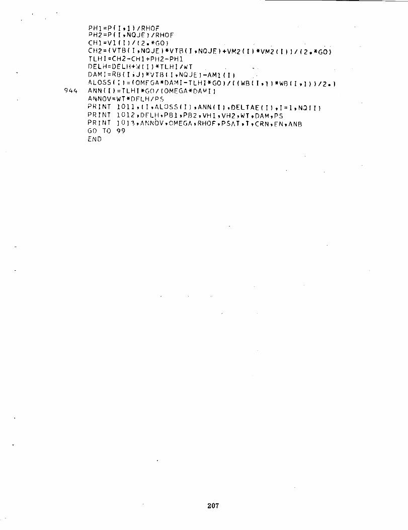
944
PHI=P(I,1)/RHOFPH2=PII,NOJEI/RHOF
CH]=VIIII/I2.*GO}
CH2=(VTB(I,NQJE)*VTB(I,NQJEI+VM2II)*VM2(I)}/(2.*GO)TLHI=CH2-CHI+PH2-PH1DELH:DELI_+WII)*TLHI/WT
DAMI=RB(I,jI*IVTBII,NQJE)-AMI(1)
ALOSSIII=(OMFGA*DAMI-TLHI*GOIIIIWBII,II*WB(I,I))/2.)
ANNIII=TLHI_GO/IOMEGA*DAMI)
ANNOV=WT*DFLH/PS
PRINT IOII,(I,ALOSS(1),ANN(II,DELTAE(II,I=I,N3II}
PRINT 1012 ,DELH,PBI,PB2,VHI ,VH2,WT,DAM,PS
PRINT I0 ]3,ANNOV,CMEGA,RHOF,PSAT ,T ,CRN,FN,ANB
GO TO 99
END
207

C
C
C
C
C
CC
C
C
C
CC
C
SUBROUTINE ANNIIL
SUBROUTINE FOR ANNULUS VELOCITY DIAGRAMS AND OTHER FLUID DATA
FOR GIVEN STREAMLINE.POSITIONS
DIMENSION Z(11,22) ,R{ 11,22} ,AN(] 1,22) tDHP(22)
COMMON AN,RR,ZZ,R,Z,TPP,TSStPBl,PB2,WBI,WB2'RHOBI'RHOB2'RHOF'PSAT'
1GO ,ANB tP IE ,AK2 ,T ,P,HP, J ,NQI ,NOJ _.V,FC ,pFR ,FSA ,SBF2 ,CBF2 ,TBP, TBS, TDB
2RB2 ,RVTI , ISTART ,AW,VBT2 ,OMEGA ,AC2,VBM2 tCNV
L=ORHOB2=RHOF
AP=O,1
ATT=RHOF _-
ADP=O,I
48 VBM2=AW/(RHOB2*AC2*ANB)
WR2=VBM2/SBF2VBT2=OMEGA*RB2-WB2*CBF2
WDR=(WBI+WB2)/2,
AK2=FSA*(RB2_VRT2-RVTI)
RHOB]2=(RHOB]+RHOB2)/2.
IF(V)I,I,4
I ALI2=0,O
GO TO 5
BEGIN LOSS CALCULATION
4 IF(WBI-WB2)6'6,7
7 AK=(I'-WB2/WBI)/(2"*(I'+WB2/WBI))
ALI2=FC_WDBWWDB+AK*(WBI_WBI-WB2 *WB2}
GO TO 5
6 AL12=FC *WDB*_!DB
5
55
8
12
9
COMPLETE LOSS CALC[JLATION
pB2=PB]+(RHOEI2/GO)*(FR-ALI2-,5*(WB2*WB2-WBI*WBI) )
IF (T)40,4(),55
PDB = (PB2+PB I )/2 •
AK3=AK2*WDB-AK2*AK2*TDB
IF(AK2 )8,9,10
[F (RHOF-RHOB2 )61,6 ] ,] 2
I_-(AP-O,OOI.) 9,9, ] 5
L=IOO
IF (PDB-PSAT) 16,17,17
ENTER TWO-PHASE FLOW ITERATION LOOP
16 RHODB=R HOF/(I"+TW(PSAT-pDB) )
GO TO 41
17 RHODB=RHOF
GO TO 41
!0 TBW=TDB-WDB/AK2
WS=WDB+AK 2 W (TBS-T DB )
IF(TBP-T_W)]9,2fl,20
19 WP=O.OTBPP=TBWGO TO 2]
2C, TBPP=TBPWP=WDB-AK2* ( TDR-T BPP )
21 IFIPDB-PSAT)22,23,24
22 RHOTDB=RHOF/(1.+T W(PSAT-PDB} )
208

WSAT2=WDB*WDB -(GO*RHOFIT)*II,IIRHOTDB*RHOTDB)-I,IIRHOF*RHOFII
lF (WSAT 2-WP*WP )25,25,26
26 WTBSAT=SQRTIWSAT2 1
29 TBSAT=TDB+IWTBSAT-WDBIIAK2 _
GO TO 27
214 WTBSAT=SQRT{ {2.*GO/RHOFi*IPDB-PSATI+WDB*WDBI
IF IWTBSAT-W£ 129,28,28 :
28 RHODR=RHOF
GO TO 4l '_
23 NN=I
XI=TDB
X2=TRS
AI=I2,*T/IGO*RHOFI I*(-AK3*TDB-,5*AK2*AK2*TDB *TDBI+I"/(RHOF*RHOF)
GO TO 31
27 NN=2
XI=TBSAT
X2=TBSAI=(2.*TIIGO*RHOFI I*I-AK3*TBSAT--5*AK2*AK2*TRSAT*TBSATI+I"IIRHOF*R
IHOF I
GO TO 3!
25 NN=3
Xi =T-_PP
X2=TBS
AI=(2.*T/(GO*RHOFI }*I-AK3*TDB-.5*AK2*AK2*TDB*TDBI+I'/(RHOTDB*RHOTD
IB)DD=SQRT(I./( {2._T/IGO*RHOF} }*(AK3*ITRPP-Tr)BI+.5*AK2*AK2*ITBPP*TR'PP
I-TDB*TDB} )+i. / IRHOTDB*RHOTDB I } }
31 B I=2.*T*AK3/{ GOI_RHOF 1
C ]=2,*T*AK2_AK2 / (GO*RHOF*2 • }
CAPXI = A I+RI.*X ] +C ]*X I*X 1
CAPX2=A ]+B],_X2+C I*X2*X2
CONSTI=I I./SQRTICI) I*ALOG(SQRT(CAPXII+XI*SQRTIC]I+BI/(2.*SQRT(C] ) )
1)CONST2=II./SQRT(CI) )*ALOGISQRTICAPX2)+X2*SQRT(CII+B1/(2"*SQRT(CI) )
1)
GO TO 132,33,341,NN32 AA=RHOF*(TDB-TBPP)+CONST2-CONST1
GO TO 30
33 AA=RHOF*(TBSAT-TBPP)+CONST2-CONST]
GO TO 30
34 AA=CONST2-C.ONST ]35 IF (T_P-TBW)36,37,37
36 RHOP=DDGO TO 38
30 IF(TRP-TBWI39,37,37
39 RHOP=RHOFGO TO 38
37 RHOP=O°O
38 RHODB=RHOP*(TBPP-TBP)/(TBS-TBP}+AA/(TBS-TBP)
4] IFIABSI(RHODB-RHOB12)/RHOB121-O.COI)61.,61,42
42 IF (L-I00)43,44,44
44 CNV=O,
GO TO 40
43 I F ( RHODR-RHOP, 12 ) 45961 , 46
46 IF(L)61,61,15
45 I F (L) 70] 1,71"_1,70270,1 TT=RHOB2
TTP=ATTBTT=RHODB
ATT=RHOBt2
209
7O2
711
707
50
ADPGOIF(IF{IF(L=LRHOGO
=APTO 5oAP-O.O01 )701,701,71 1
AP-ADP)701,707,707
RHOB12-RHODB-ATT+BTT}701,62,62
+l
B2=TT*(I.-AP)TC 48
62 TT=2.WTTP-RHOB]
15 AP=AP/IO.GO TO 5O
61CNV=I.40 RETURN
END
210

CC
C
SUBROUTINE BLADE
SUBROUTINE FOR
DIMENSION Z(11,COMMON AN,RR,ZZ
1GO,ANB,P I E ,AK2*
2RL_2,RVTI,ISTART
1,906 FORMATIBFIO.4)
1007 FORMAT(IP8ElS.7
GO TO (I,6,5,10
1 READ 1006,
ITF(3)
BLADE SURFACE COORDINATES TP AND TS FROM GIVEN R,Z
22),RIII,22),AN|II,22),DHP(22),T_(22)
,R,Z,TPP,TSS,PBI,PB2,WBI,WB2,RHOBI,RHOB2,RHOF,PSAT,
T,DHP,J,NOI,NQJ,V,FC,FR,FSA,SBF2,CBF2,TSP,TBS,TDB,
,AW,VBT2,0MEGA,AC2,VBM2,CNV
)
,8,11),ISTART
AA,BB,CC,DSEX,TIT,RIT,DTR,ANB,TF(]),TF(2),
PRINT IO07,AA,BB,CC,DSEX,TIT,RIT,DTR,ANB,TF(1),TF(2),
]TF(3)
IF (NQJ-4) 75,76,76
76 DO 2_ K=4,NQJ
23 TF(K)=I.
75 TPNB=2.*PIE/ANB
DO 24 K=I,NQJ
TTH=TF(K}_(T1T+DTR*(R1T-R(1,K) ) )
TTT=TF(K)*(TITt.DTR*(RIT-R(NQI,K)) )
DZf)T=AA+BB'wZ(NQI,K)+CC*Z(NQI,K)*Z(NQI,K)
ADHP=TPNBWDZDT
ADH=ADHP-TTT
BDH=ADHP-TTH
CDH=AN ( NO I ,K )
24 Dt4P (K) = ]. / ( 1. / (2, WCDH) +1. / (ADH+BDH) )DO 27 K=2,NQJ
21 DHP(K) =(DHP(K-] )+DHP(K) )/2.IF(CC)3,4,3
4 IF(BB)25,26,25
2,6 ISTART=2
GO TO 6
25 ISTART=3
GO TO 5
3 O=4.*AAwCC-BR*BRIF(017,28,9
28 ISTART=5
GO TO 8
7 SO=SORT(-O)
RSO=] .ISO
BMSO=BB-SO
BPSQ=BB+SO
FBSO=BMSO/BPSQISTART=4
GO TO 109 SO=SORT(O)
$02=2./SO
TQ=SQ2*ATAN ( RB/SQ )
ISTART =6
GO TO 11
6 TPP=-ZZIAA
RSBB=RR*S IN (ATAN (AA/RR ) }
GO TO 30
5 TPP=(-I./BB)*ALOG((AA+BB*ZZ)/AAI
RSBB=RR*S IN(ATAN((AA+BB*ZZ)/RR))GO TO 30
10 TPP=-RSQ*ALOG( ((2._CCwZZ+BMSQ)I(2.*CCwZZ+BPSQ))IFBSQ)
31 RSBB=RR*SIN(ATAN( (AA*B_*ZZ+CC*ZZwZZ)/RR)}
211
8
11
3O
GO TO 30Tpp=(I./(BB+CC_ZZII-I./BB
GO TO 31Tpp=-sQ2_(ATANII2._CC_ZZ+BB)/SQ)I+TQGO TO 31TT=T1T+DTR_IR1T-RR)TTF=TT_TFCJIAJ=J-1QQJ=NQJ-I
TDS=2._DSEX_IAJ/OQJ}TSS=Tpp+TPNB-(TTF+TI)S)IRSBB
RETURN
END
}
t
i
212
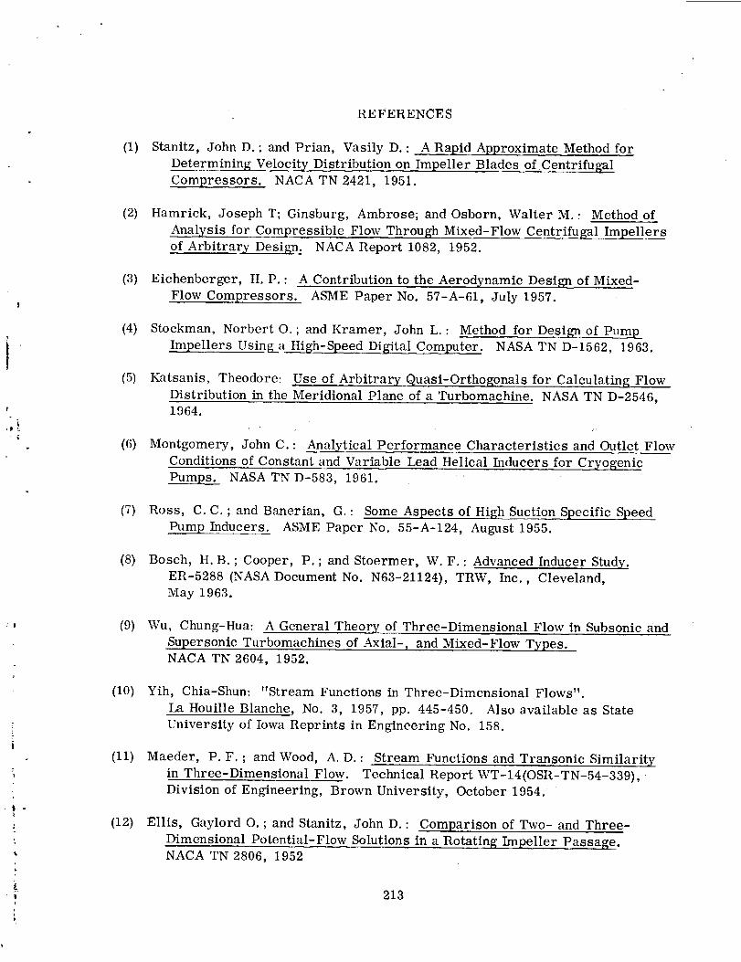
|
(1)
(2)
(3)
(4)
REFERENCES
Stanitz, John D. ; and Prian, Vasily D. : A Rapid Approximate Method for
Determining Velocity Distribution on Impeller Blades of Centrifugal
Compressors. NACA TN 2421, 1951.
Hamrick, Joseph T; Ginsburg, Ambrose; and Osborn, Walter M, : Method of
_Analysis for Compressible Flow Through Mixed-Flow Centrifugal Impellers
of Arbitrary Design_. NACA Report 1082, 1952.
Eichenberger, H. P. : A Contribution to the Aerodynamic Design of Mixed-
Flow Compressors. ASME Paper No. 57-A-61, July 1957.
Stockman, Norbert O. ; and Kramer, John L. : Method for Design of Pump
Impellers Using_a_h--_d__tal Com utp__u_t_. NASA TN D-1562, 1963.
(5) Katsanis, Theodore: Use of Arbitrary. Quasi-Orthogonals for Calculating Flow
Distribution in the Meridional Plane of a Turbomachine. NASA TN D-2546,1964.
(6) Montgomery, John C. : Analytical Performance Characteristics and Outlet Flow
Conditions of Constant and Variable Lead Helical Inducers for Cryogenic
(7)
(s)
(9)
(10)
(11)
(12)
Pure sp___ NASA TN D-583, 1961.
Ross, C. C. ; and Banerian, G. : Some Aspects of High Suction Specific SpeedPump Inducers. ASME Paper No. 55-A-124, August 1955.
Bosch, H.B. ; Cooper, P. ; and Stoermer, W. F. : Advanced Inducer Study.
ER-5288 (NASA Document No. N63-21124), TRW, Inc., Cleveland,May 1963.
Wu, Chung-Hua: A General Theory of Three-Dimensional Flow in Subsonic and
Supersonic Turbomachines of Axial-, and Mixed-Flow Types.NACA TN 2604, 1952.
Yih, Chia-Shun: "Stream Functions in Three-Dimensional Flows".
La Houille Blanche, No. 3, 1957, pp. 445-450. Also available as State
University of Iowa Reprints in Engineering No. 158.
Maeder, P.F. ; and Wood, A. D. : Stream Functions and Transonic Similarity
in Three-Dimensional Flow. Technical Report WT-14(OSR-TN-54-339),
Division of Engineering, Brown University, October 1954.
Ellis, Gaylord O. ; and Stanitz, John D. : Comparison of Two- and Three-
Dimensional Potential-Flow Solutions in a Rotating Impeller Passage.NACA TN 2806, 1952
213

(13)
(14)
(15)
(16)
(17)
(18)
(19)
Stahl, H. A. ; and Stepanoff, A.J. : Thermodynamic Aspects of Cavitation in
Centrifugal Pumps. ASME Paper No. 55-A-136, November 1955.
Stepanoff, A.J. : Cavitation Properties of Liquids. ASME Paper No.
63-AHGT-22, March 1963.
Vavra, M.H. : Aero-Thermodynamics and Flow in Turbomachines. John
Wiley & Sons, Inc., 1960.
Ruggeri, Robert S. ; and Gelder, Thomas F. : Effects of Air Content and
Water Purity on Liquid Tension at Incipient Cavitation in Venturi Flow.
NASA TN D-1459, 1963.
Salemann, Victor: Cavitation and NPSH Requirements of Various Liquids.
ASME Paper No. 58-A-82, December 1958.
Spraker, W. A. : The Effects of Fluid Properties on Cavitation in
Centrifugal Pumps. ASME Paper No. 64-WA/FE-14, December 1964.
Roder, Hans M. ; and Goodwin, Robert D. : Provisional Thermodynamic
Functions for Para-Hydrogen. NBS TN-130, 1961
(20) Keenan, Joseph H. : Thermodynamics. John Wiley & Sons, Inc., 1956,
p. 329.
(21) Marks, L.S. : Mechanical Engineers' Handbook. Fifth Edition, McGraw-Hill
Book Co., Inc., 1951, p. 250.
(22) Stanitz, John D. : Two Dimensional Compressible Flow in Turbomachines
(23)
(24)
(25)
(26)
with Conic Flow Surfaces. NACA Report 935, 1949.
Kramer, James J. ; Stockman, Norbert O. ; and Bean, Ralph J.: Nonviscous
Flow Through a Pump Impeller on a Blade-to-Blade Surface of Revolution.
NASA TN D-1108, 1962.
Kramer, James J. ; Stockman Norbert O. ; and Bean, Ralph J. : Incompressible
Nonviscous Blade-to-Blade Flow Through a Pump Rotor with Splitter Vanes,
NASA TN D-1186, 1962.
Martin, M. H. : "On the Uniqueness of Harmonic Functions Under Boundary
Conditions". Journal of Mathematics and Physics, Volume 17, No. 1,
March 1963, pp. 1-13.
Levin, Simon A. : Uniqueness and Nonlinearity. Technical Note BN-354
(NASA Document No. N64-25777, DDC No. AD-602033), University of
Maryland, May 1964.
214

(27)
(28)
(29)
(30)
(31)
(32)
(33)
(34)
(35)
(36)
(37)
(38)
(39)
(40)
Crandall, StephenH. :1956.
Engineering Analysis. McGraw-Hill Book Co., Inc.,
Whittaker, E.; and Robinson, G. : The Calculus of Observations. Fourth • •
Edition, Blackie & Son Limited, 1956.
Marquardt, Donald W. :
linear Parameters".
pp. 431-441.
"An Algorithm for Least-Square Estimation of Non-
SIAM Journal, Volume 11, No. 2, June 1963,
Goldfeld, Stephen M. ; Qtlandt, Richard E. ; and Trotter, Hale F. :
Maximiation by Quadratic Hill-Climbing, 'Research Memorandum No. 72,
Princeton University Econometric Research Program, January 1965.
Soltis, Richard F. ; Anderson, Douglas A. ; and Sandercock, Donald M. :
Investigation of the Performance of a 78 ° Flat-Plate Helical Inducer.
NASA TN D-1170, 1962.
Adams, Harold E. : PumpingBoiling Fluids When the Available Static Head
is Zero or Less. ASME Paper No. 63-WA-220, November 1963.
Johnsen, Irving A. ; and Bullock, Robert O., editors: Aerodynamic Design of
Axial-Flow Compressors. Volume I. NACA RM E56B03, 1956.
Stripling, L. B. ; and Aeosta, A.j. : Cavitation in Turbopumps- Part I.
ASME Paper No. 61-WA-112, December 1961.
Stripling, L.B. : Cavitation in Turbopumps - Part 2. ASME Paper No. 61 -WA-98, December 1961.
Jakobsen, J. K. : On the Mechanism of Head Breakdown in Cavitating Inducers.
ASME Paper No. 63-AHGT-29, March 1963.
Gouse, S.W. Jr. ; and Brown, George A.: A Survey of the Velocity of Sound
in Two-Phase Mixtures. ASME Paper No. 64-WA/FE-35, December 1964.
Smith, R.W. : Some Idealized Solutions for Choking, _Two-Phase Flow of
Hydrogen, Nitrogen and Oxygen. Adv. in Cryogenic Engineering, Volume 8,
New York, Plenim Press, 1963, pp. 563-573.
Sandercock, Donald M. ; Soltis, Richard F. ; and Anderson, Douglas A. :Cavitation and Noncavitation Performance of an 80.6 ° Flat-Plate
Helical Inducer at Three Rotational Speeds. NASA TN D-1439, 1962.
Ruggeri, Robert S. ; and Gelder, Thomas F. : Cavitation and Effective
Liquid Tension of Nitrogen in A Tunnel Venturi. NASA TN D-2088, 1964.
215

(41) Gelder, Thomas F. ; and Ruggeri, Robert S.: Incipient Cavitation of Freon-114 in a Tunnel Venturi. NASA TN D-2662, 1965.
(42) Holl, William J. ; and Treaster, A. L. : Cavitation Hysteresis. ASME Paper
No. 65-FE-9, June 1965.
(43) Apostol, Tom M. : Calculus. Volume II. Blaisdell Publishing Co., 1962.
(44) Spiegel, Murray R. : Vector Analysis. Schaum Publishing Co., 1959.
(45) Benton, Thomas C. : "An Example of the Need for Two Stream Functions inThree-Dimensional Flows". Quarterly Applied Mathematics, Volume
21, No. 3, October 1963, pp. 235-237.
216

DISTRIBUTION LIST
Cg_pie s Recipient
NASA Headquarters, Washington, D.C. 20546
Contracting Officer, BCA
Patent Office, AGP
NASA Lewis Research Center
21000 Brookpark Road, Cleveland, Ohio 44135
Office of Technical Information
Contracting OfficerPatent Office
NASA Marshall Space Flight Center
Huntsville, Alabama 35812
Office of Technical Information, M-MS-IPC
Purchasing Office, PR-CH
Patent Office, M-PAT
Keith Chandler, R-P&VE-PA
NASA Western Operations Office
150 Pico Boulevard, Santa Monica, California 90406
Office of Technical Information
Contracts Management Division
General Counsel for Patent Matters
Chief, Liquid Propulsion Technology, RPL
Office of Advanced Research and Technology
NASA Headquarters
Washington, D.C. 20546
26 NASA Scientific and Technical Information FacilityP.O. Box 33
College Park, Maryland 20740
Mr. Vincent L. Johnson
Director, Launch Vehicles and Propulsion, SV
Office of Space Science and Applications
NASA Headquarters, Washington, D.C. 20546
Mr. Edward L. Gray
Director, Advanced Manned Missions, MT
Office of Manned Space Flight
NASA Headquarters, Washington, D.C. 20546
217
DesD._rnee
( )( )
(x)(x)(x)
( )( )( )( )
( )( )( )
(x)
(x)
(x)
(x)

1
10
Receipient
Mr. Clarence A. Syvertson
Mission Analysis Division
NASA Ames Research Center
Moffett Field, California 24035
(Technical Monitor)Mr. Werner Britsch
Lewis Research Center
Cleveland, Ohio 44135
Mr. Loren Gross
Marshall Space Flight Center
Huntsville, Alabama 35812
Designee
(x)
(x)
218
NASAFIELD CENTERS
Copies Recipient
2 Ames Research Center
Moffett Field, California 94035
Goddard Space Flight Center
Greenbelt, Maryland 20771
Jet Propulsion Laboratory
California Institute of Technology4800 Oak Grove Drive
Pasadena, California 91103
Langley Research Center
Langley Station
Hampton, Virginia 23365
2 Lewis Research Center
21000 Brookpark Road
Cleveland, Ohio 44135
Marshall Space Flight Center
Huntsville, Alabama 35812
Manned Spacecraft Center
Houston, Texas 77001
Western Operations Office150 Pico Boulevard
Santa Monica, California 90406
John F. Kennedy Space Center, NASACocoa Beach, Florida 32931
Designee
Harold Hornby
Mission Analysis Div.
Merland L. Moseson
Code 620
Henry Burlage, Jr.
Propulsion Div., 38
Dr. Floyd L. ThompsonDirector
Dr. Abe Silverstein
Director
Hans G. Paul
Code R-P&VED
Dr. Robert R. Gilruth
Director
Robert W. Kamm
Director
Dr. Kurt H. Debus
219

GOVERNMENTINSTALLATIONS
Copies Recipient
Aeronautical Systems Division
Air Force Systems Command
Wright-Patterson Air Force Base
Air Force Missile Development Center
Holloman Air Force Base, New Mexico
Air Force Missile Test Center
Patrick Air Force Base, Florida
Air Force Systems Division
Air Forc'e Unit Post Office
Los Angeles 45, California
Arnold Engineering Development Center
Arnold Air Force Station
Tullahoma, Tennessee
Bureau of Naval Weapons
Department of the Navy
Washingtbn, D. C.
Defense Documentation Center Headquarters
Camerson Station, Building 5
5010 Duke Street
Alexandria, Virginia 22314
ATTN: TISIA
Headquarters, U.S. Air Force
Washington 25, D.C.
Picatinny Arsenal
Dover, New Jersey 07801
Air Force Rocket Propulsion Laboratory
Research and Technology Division
Air Force Systems Command
Edwards, California 93523
Designee
D.L. Schmidt
Code ASRCNC-2
I
Maj. R.E. BrackenCode MDGRT
L.J. Ullian
Col. Clark
Technical Data
Center
Dr. H.K. Doetsch
J. KayRTMS-41
Col. C.K. Stambaugh
- AFRST
I. Forsten, Chief
Liquid Propulsion Laboratory,
SMUPA-DL
RPRR/Mr. H. Main
220

GOVERNMENT INSTALLATIONS
C__opies Recipient
U.S. Atomic Energy CommissionTechnical Information Services
Box 62
Oak Ridge, Tennessee
U.S. Army Missile CommandRedstone Arsenal
Alabama 35809
U.S. Naval Ordnance Test Station
China Lake
California 93557
Designee
A.P. Huber
Oak RidgeGaseous Diffusion Plant
(ORGDP) P O. Box P
Dr. Walter Wharton
Code 4562
Chief, Missile
Propulsion Div.
CPIA
1 Chemical Propulsion Information Agency
Applied Physics Laboratory
8621 Georgia Avenue
Silver Spring, Maryland 20910
Nell Safeer
221

INDUSTRYCONTRACTORS
Copies
1
Recipient
Aerojet-General CorporationP.O. Box 296
Azusa, California 91703
Aeroj et- General CorporationP.O. Box 1947
Technical Library, Bldg. 2015, Dept.
Sacramento, California 95809
Aeronautronic
Philco Corporation
Ford Road
Newport Beach, California 92663
Aerospace Corporation2400 East E1 Segundo Blvd.
P.O. Box 95085
Los Angeles, California 90045
Arthur D. Little, Inc.
20 Acorn Park
Cambridge, Massachusetts 02140
Astropower Laboratory
Douglas Aircraft Company2121 Paularino
Newport Beach, California 92663
Bell Aerosystems Company
P.O. Box 1
Buffalo, New York 14240
Northrop Space Laboratories
3401 West Broadway
Hawthorne, California
Stanford Research Institute
333 Ravenswood Avenue
Menlo Park, California 94025
TRW SystemsTRW Incorporated
One Space ParkRedondo Beach, California 90278
222
2410
Designee
L.F. Kohrs
R. Stiff
D.A. Carrison
John G. Wilder
MS-2293
Propulsion Dept.
E. Karl Bastress
Dr, George MocDirector, Research
W.M. Smith
Dr. William Howard
Lionel Dickinson
G.W. Elverum
INDUSTRYCONTRACTORS
!
Copies
1
Recipient
Research LaboratoriesUnited Aircraft Corporation400 Main StreetEast Hartford, Connecticut06108
Bendix SystemsDivisionBendix Corporation3300Plymouth RoadAnn Arbor, Michigan
Boeing CompanyP.O. Box 3707Seattle, Washington98124
Missile DivisionChrysler CorporationP.O. Box 2628Detroit, Michigan 48231
Wright Aeronautical DivisionCurtiss-Wright CorporationWood-Ridge, New Jersey 07075
Missile and SpaceSystemsDivisionDouglas Aircraft Company, Inc.3000OceanPark BoulevardSantaMonica, California 90406
Aircraft Missiles DivisionFairchild Hiller CorporationHagerstown, Maryland 10
General Dynamics/AstronauticsLibrary & Information Services (128-00)P.O. Box 1128SanDiego, California 92112
Re-Entry Systems DepartmentGeneral Electric Company3198Chestnut StreetPhiladlphia, Pennsylvania19101
Designee
Erle Martin
John M. Brueger
J.D. Alexander
John Gates
G. Kelley
R.W. HalletChief EngineerAdvancedSpaceTech.
J.S. Kerr
Frank Dore
F.E. Schultz
223

INDUSTRYCONTRACTORS
1 AdvancedEngine & Technology Dept.General Electric CompanyCincinnati, Ohio45215
Grumman Aircraft Engineering Corp.Bethpage, Long IslandNew York
LockheedCalifornia Company2555North HollywoodWayBurbank, California 91503
LockheedMissiles and SpaceCo.Attn: Technical Information CenterP.O. Box 504Sunnyvale, California 94088
LockheedPropulsion CompanyP.O. Box 111Redlands, California 92374
The Marquardt Corporation16555Staticoy StreetVanNuys, California 91409
Baltimore DivisionMartin Marietta CorporationBaltimore, Maryland 21203
Denver DivisionMartin Marietta CorporationP.O. Box 179Denver, Colorado 80201
McDonnell Aircraft CorporationP.O. Box 516Municipal AirportSt. Louis, Missouri 63166
Space & Information Systems DivisionNorth American Aviation, Inc.12214LakewoodBoulevardDowney, California 90241
224
Designee
D. Suichu
Joseph Gavin
G.D. Brewer
Y.C. Lee
H.L. Thackwell
Warren P. Boardman, Jr.
John Calathes {3214)
J.D. Goodlette (A-241)
R. A Herzmark
H. Storms

INDUSTRYCONTRACTORS
C__pies Recipient
Rocketdyne (Library 586-306)
North American Aviation, Inc.
6633 Canoga Avenue
Canoga Park, California 91304
United Technology Center587 Methilda Avenue
P.O. Box 358
Sunnyvale, California 94088
Aerospace Operations
Walter Kidde and Company, Inc.567 Main Street
Belleville, New Jersey 07109
Florida Research and Development
Pratt and Whitney Aircraft
United Aircraft Corporation
P.O. Box 2691
West Palm Beach, Florida 33402
Rocket Research Corporation520 South Portland Street
Seattle, Washington 98108
Pennsylvania State UniversityP.O. Box 30
State College, Pa. 16801
Iowa State University
Department of Mechnical EngineeringAmes, Iowa
Worthington Corporation
401 Worthington Avenue
Harrison, New Jersey 07029
Designee
E.B. Monteath
B. Abelman
R.J. Hanville
Director of Research
Engineering
R.J. Coar
Foy McCullough, Jr.
Dr. Wislicenus
Dr. Serovy
Mr. Walter Jekat
225

l
!f
: {
I


