
THREE - DIMENSIONAL GEOMETRIC NONLINEAR CONTACT STRESS
ANALYSIS OF RIVETED JOINTS/N -3
Final Report
Submitted to
NASA Langley Research Center
Hampton, VA
NASA Grant No. NAGl-1754
September 18, 1995 through September 30,1998
By
Dr. Kunigal N. Shivakumar and Vivek Ramanujapuram
Center for Composite Materials Research
Department of Mechanical Engineering
North Carolina A & T State University
Greensboro, North Carolina
1998
https://ntrs.nasa.gov/search.jsp?R=19990031966 2018-05-07T22:57:27+00:00Z
TABLE OF CONTENTS
TABLE OF CONTENTS ..................................................................................................... I
LIST OF FIGURES ............................................................................................................. 4
LIST OF TABLES ............................................................................................................... 8
1 INTRODUCTION ................................................................................................... 9
1.1 Introduction .................................................................................................. 9
1.2 Background ................................................................................................... 9
1.3 Total Fatigue Life Prediction Models ........................................................ 12
1.4 Rivet Clampup and Interference ................................................................ 13
1.5 Problem Definition ..................................................................................... 14
1.6 Objectives of Research ............................................................................... 16
1.7 Scope .......................................................................................................... 16
2 FINITE ELEMENT ANALYSIS ............................................................................ 18
2.1 Introduction ................................................................................................ 18
2.2 Finite Element Analysis .............................................................................. 18
2.3 Finite Element Modeling of Rivet Joint ....................................................... 20
2.3.1 CONTAC49 Element Description .................................................. 21
2.4 Modeling of Clampup ................................................................................. 30
2.5
2.6
2.7
2.8
2.9
Modeling of Interference ............................................................................ 31
Modeling of The Combined Case ............................................................... 31
Analysis Procedure ..................................................................................... 32
Convergence Criteria ................................................................................... 32
Summary .................................................................................................... 34
4
PIN JOINTANALYSIS.........................................................................................35
3.1 Introduction................................................................................................35
3.2 JointConfiguration.....................................................................................35
3.3 AnalysisModel...........................................................................................35
3.4 AnalysisCases............................................................................................36
3.4.1 ElasticFriction................................................................................37
3.4.2 PinClamp-up:.................................................................................37
3.4.3 PinInterference:..............................................................................37
3.4.4 CombinedCase...............................................................................37
3.5 Results........................................................................................................38
3.5.! NeatFit Results..............................................................................38
3.5.1.! DeformedShapes...................................................38
3.5.1.2 ContactNonlinearity...............................................38
3.5.1.3 RadialStressDistributionattheHoleBoundary....39
3.5.1.4 HoopStressDistributionattheHoleBoundary.....40
3.5.1.5 HoopStressContourPlots.....................................40
3.5.2 ClampupForce...............................................................................40
3.5.3 Interference.....................................................................................41
3.5.4 CombinedCase...............................................................................4!
3.6 Summary....................................................................................................41
TWO RIVET ANALYSIS ...................................................................................... 63
4.1
4.2
4.3
4.4
Introduction ................................................................................................ 63
Joint Configuration ..................................................................................... 63
Analysis Model ........................................................................................... 64
Analysis Cases ............................................................................................ 68
4.4.1
4.4.2
4.4.3
Friction:..........................................................................................69
RivetClamp-up:..............................................................................69
RivetInterference:...........................................................................69
4.5 Results........................................................................................................70
4.5.1 NeatFit Results..............................................................................70
4.5.1.1 DeformedShapes...................................................70
4.5.1.2 ContactNonlinearity...............................................70
4.5.1.3 RadialStressDistributionattheHoleBoundary....71
4.5.1.4 HoopStressDistributionattheHoleBoundary.....71
4.5.1.5 HoopStressContourPlots.....................................72
4.5.2 ElasticFriction................................................................................72
4.5.3 ClampupForce...............................................................................73
4.5.4 CIampupandElasticFriction..........................................................74
4.5.5 Interference.....................................................................................75
4.6 Summary....................................................................................................76
ELASTIC- PLASTICANALYSIS......................................................................110
5.1 Introduction..............................................................................................110
5.2 MaterialModeling....................................................................................110
5.3 Analysis....................................................................................................111
5.4 ResultsandDiscussion.............................................................................111
5.5 Summary..................................................................................................113
CONCLUDING REMARKS..............................................................................123
REFERENCES.....................................................................................................126

Figure Page
1.1
1.2
1.3
2.1
LIST OF FIGLq_ES
2.2
2.3
2.4
2.5
2.6
2.7
2.8
3.1
3.2
3.3
3.4
3.5
3.6
3.7
3.8
3.9
3.10
Pin joint .................................................................................................................. 15
Two rivet single lap joint ..................... _................................................................... 15
Experimental panel .................................................................................................. 16
Representation of a two-dimensional solid as an assemblage of triangular ................finite elements ......................................................................................................... 20
The CONTAC49 element configuration ................................................................. 23
Definition of Near-Field and Far-Field Contact ........ i............................................. 24
Pseudo Element ...................................................................................................... 25
Target Co-ordinate Systems .................................................................................... 26
Location of contact node on the target plane ........................................................... 28
Schematic of the clampup procedure ....................................................................... 31
Schematic of the interference procedure .................................................................. 31
Joint configuration .................................................................................................. 44
Joint configuration for the finite element model ...................................................... 45
Finite element model of the pin joint ....................................................................... 46
Clampup versus contraction of pin .......................................................................... 47
Deformed shape at the pin and hole boundary. ........................................................ 48
Hoop stress vs remote stress for various z values at 0 = 90 ° ................................... 49
Stress concentration factors Vs remote stress ......................................................... 50
Membrane and bending stress components ............................................................ 51
Radial stress distribution around the hole boundary (¢J_ = 28.8 Mpa) .................... 52
Radial stress distribution around the hole boundary (_= = 156.04 Mpa) ................ 53
3.11
3.12
3.13
3.14
3.15
3.16
3.17
3.18
3.19
4.1
4.2
4.3
4.4
4.5
4.6
4.7
4.8
4.9
4.10
4.1t
4.12
4.13
4.14
4.15
Cosinefit for radialstressdistributionaroundtheholeboundary(cLo= 28.8Mpa)54
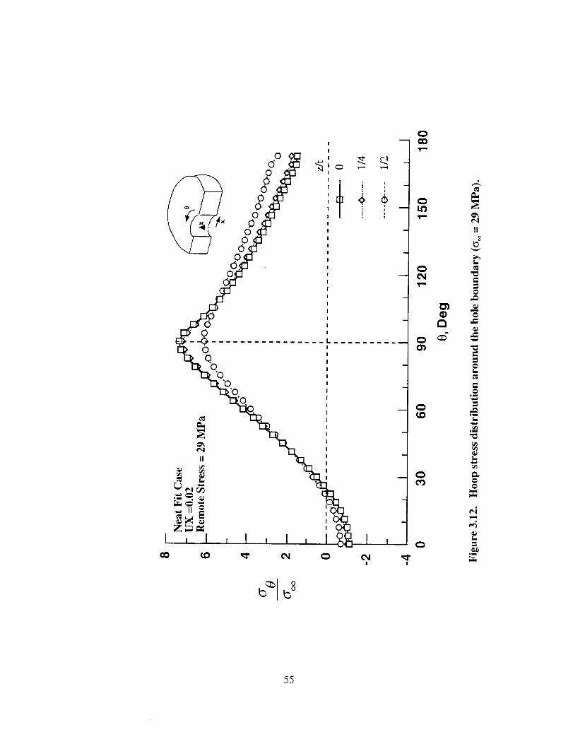
Hoopstressdistributionaroundtheholeboundary(_== 28.8Mpa).....................55
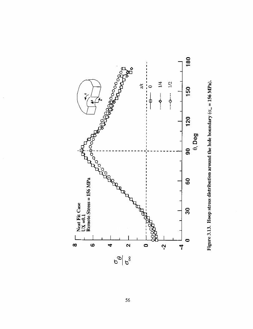
Hoopstressdistributionaroundtheholeboundary(or = 156.04Mpa).................56
Contourplotof thehoopstressin theplate(cLo= 156.04Mpa).............................57
Hoopstressvs remotestressatz = 0 and0 = 900for differentclampup.................58
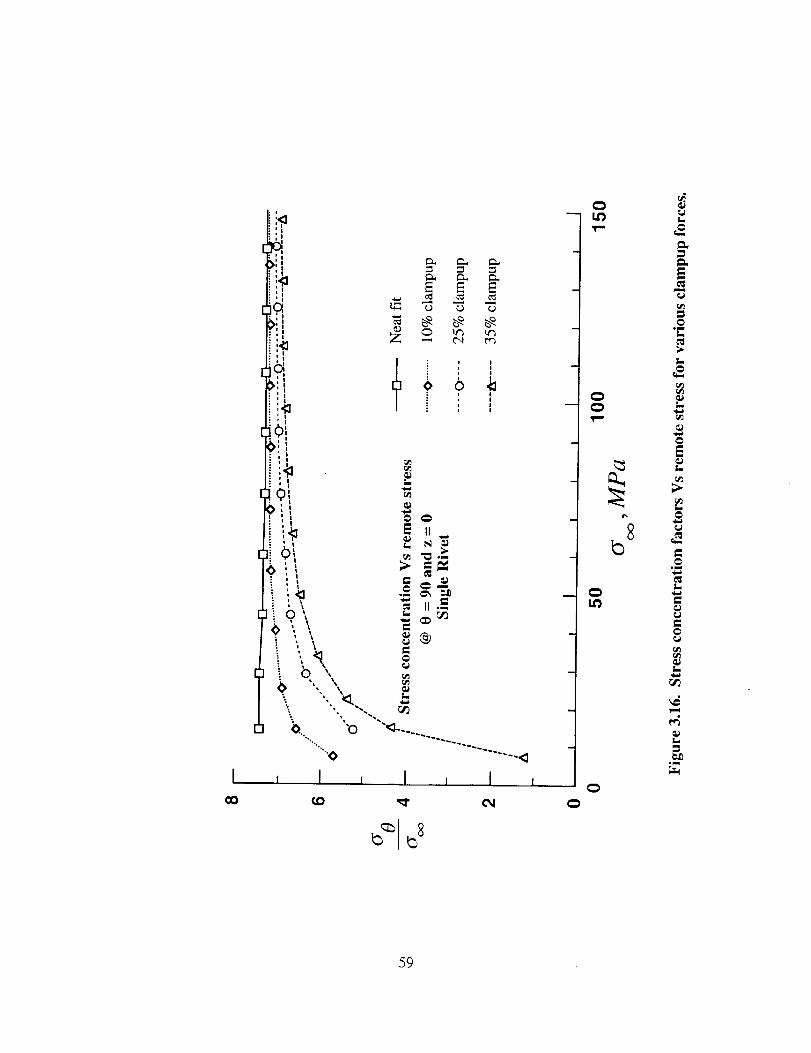
StressconcentrationfactorsVs remotestressfor variousclampupforces..............59
Hoopstressvs remotestressatz = 0 and0 = 900for elasticfriction andclampup.60
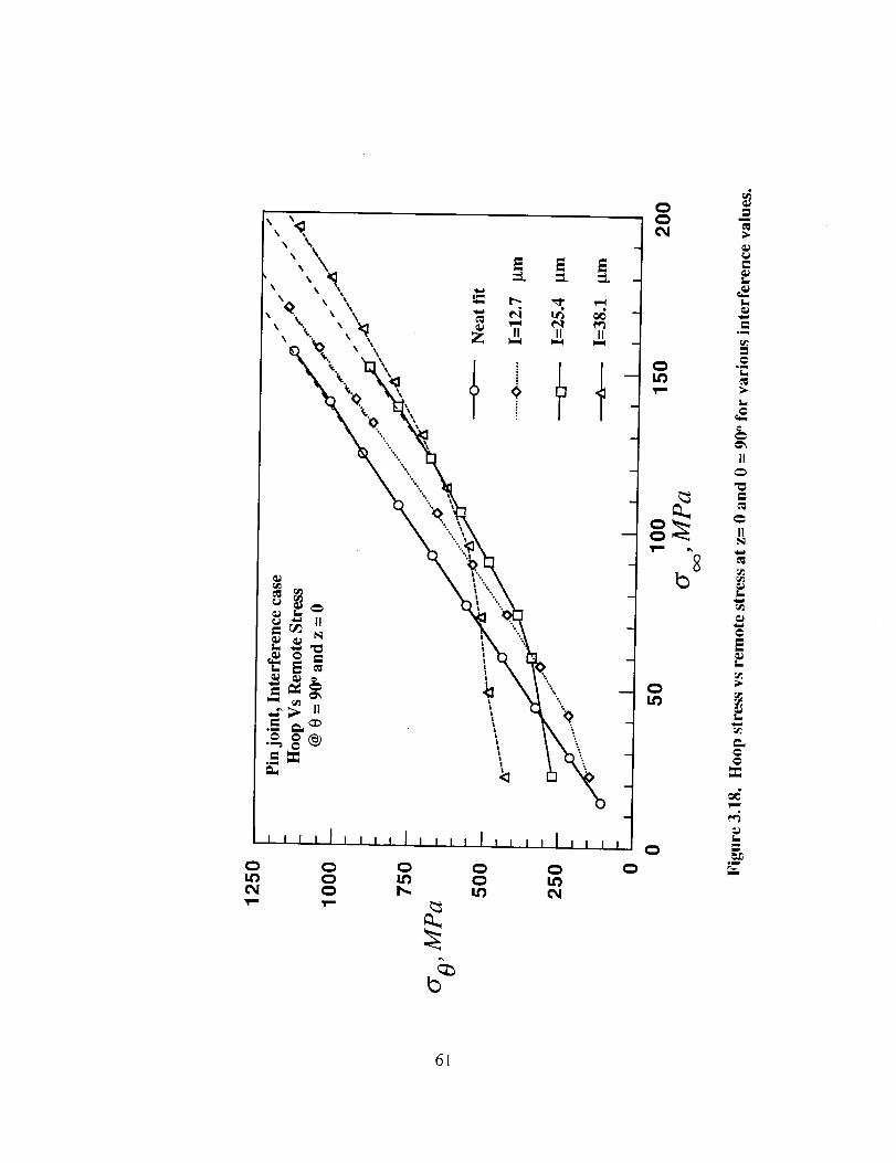
Hoopstressvs remotestressat z=0 and0 = 90° for variousinterferencevalues....61
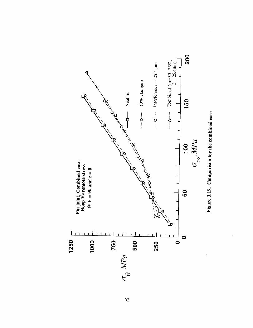
Comparisonfor thecombinedcase.........................................................................62
Isometricviewof thegeometricmodel....................................................................64
Jointconfigurationof doublerivetsinglelapjoint ..................................................64
Sectional3-Dviewshowingcyclicanti-symmetry..................................................65
Onefourthof themodel..........................................................................................66
Variousviewsof therivet,plateandthejoint finiteelementmodel..........................67
Clamp-upforceVs contraction...............................................................................67
Deformedshapeof thejoint (full view)...................................................................80
Deformedshapeof thejoint (close-upview)...........................................................81
Deformedshapeof thejoint (superimposedimage)...............................................82
Hoopstressvsremotestressfor variousz valuesat0 = 90°...................................83
Stressconcentrationvsremotestressfor variousz values.......................................84
Meanandbendingstressfor bottomplate..............................................................85
Radialstressdistributionaroundtheholeboundary(or = 45.27Mpa)..................86
Radialstressdistributionaroundtheholeboundary(or = 84.26Mpa)..................87
Hoopstressdistributionaroundtheholeboundary(o" = 45.27Mpa)...................88
4.16
4.17
4.18
4.19
4.20
4.21
4.22
4.23
4.24
4.25
4.26
4.27
4.28
4.29
4.30
4.31
4.32
4.33
4.34
4.35
5.1
5.2
5.3
5.4
Hoopstressdistributionaroundtheholeboundary(_== 84.26Mpa)...................89
Hoopstresscontourfor asectionatt3= 90°...........................................................90
Radialstressdistributionatholeboundary.............................................................9 I
Hoopstressdistributionatholeboundary..............................................................92
Hoopstressvsremotestressfor variousvaluesof _ ..............................................93
Hoopstressdistributionaroundtheholeboundary(or = 45.7).............................94
Hoopstressdistributionaroundtheholeboundary(cry,= 94.5).............................95
Hoopstressdistributionaroundtheholeboundary(or = 143.7)...........................96
Hoopstressvs remotestressatz = 0 andt3= 90° for differentclampup................97
Membranestressfor bottomplateate = 90°..........................................................98
Bendingstressfor bottomplateatt3= 900..............................................................99
Variationof hoopstressin theradialdirection......................................................I00
Clampup+ friction @0 = 90andz = 0 of bottomplate.......................................102
Hoopstressdistributionaroundtheholeboundary(or - 48.7Mpa)...................103
Hoopstressdistributionaroundtheholeboundary(or = 78.7Mpa)...................104
Radialstressdistributionaroundtheholeboundary(or = 48.7Mpa)..................105
Radialstressdistributionaroundtheholeboundary(_== 78.7Mpa)..................106
Hoopstressvs remotestressatz=0 andO= 90°..................................................107
Membranestressvsremotestressat 13= 90°........................................................108
Bendingstressvsremotestressatt9= 90°............................................................109
Uniaxialstress-strainresponseof 2024-T3Alcladaluminumalloy......................115
Subsequentyield surfacefoeisotropichardening.................................................I 16
Progressiveplasticzonewith loadingin thebottomplateof thejoint....................117
Variationof hoopstressalong19in thebottomplateato" = 50.2MPa.................118

5.5
5.6
5.7
5.8
Variationof hoopstressalong0 in thebottomplateatc®= 74.2MPa.................119
Variationof hoopstressalong0 in thebottomplateatc®= 97.7MPa.................120
Variationof hoopstressat0 = 90°with (y®...........................................................121
Variationof membraneandbendingcomponentstresseswith remotestress.............(at0 = 90° andz = O)in thebottomplate..............................................................! 22

Table
3.1
4.1
4.2
5.1
LIST OF TABLES
Page
Values of 'a' and 'n' for various values of remote stresses .................................... 39
Maximum hoop stress location in bottom plate for various clampup forces ............ 78
Maximum hoop stress location in bottom plate for different interference ............... 79
Location of maximum hoop sti'ess for bottom plate .............................................. 1 !4
1. INTRODUCTION
1.1 Introduction
Theproblemsassociatedwith fatiguewerebroughtinto theforefrontof researchby
theexplosivedecompressionandstructuralfailureof theAlohaAirlinesFlight 243in 1988.
Thestructuralfailureof this airplane has been attributed to debonding and multiple cracking
along the longitudinal lap splice riveted joint in the fuselage. This crash created what may
be termed as a minor "Structural Integrity Revolution" in the commercial transport
industry. Major steps have been taken by the manufacturers, operators and authorities to
improve the structural airworthiness of the aging fleet of airplanes. Notwithstanding this
considerable effort there are still outstanding issues and concerns related to the formulation
of Widespread Fatigue Damage which is believed to have been a contributing factor in the
probable cause of the Aloha accident. The lesson from this accident was that Multiple-Site
Damage (MSD) in "aging" aircraft can lead to extensive aircraft damage. A strong
candidate in which MSD is highly probable to occur is the riveted lap joint.
1.2 Background
Riveted lap joints are used in an aircraft fuselage to join large skin sections. Among
the many different types of joints, the single lap riveted joint is commonly used in aircraft
construction. Joining introduces discontinuities (stress raisers) in the form of holes,
changes in the load path due to lapping, and additional loads such as rivet bearing and
bending moments. Because of these changes at the joint, local stresses are elevated in the
structural component. Accurate estimations of these local stresses are needed to predict
joint strength and fatigue life.
Exhaustive studies on stress-concentration factors fSCF's) for holes and notches in
two-dimensional bodies subjected to a wide variety of loadings have been reported in the
9
literature[1,2]. Studieshavealsobeenmadeonthree-dimensionalstress-concentrationsat
circularholesin platessubjectedto remotetensionloads[3-6]. A paperby Foliasand
Wang[6] providedareviewof theseprevioussolutionsandpresentsa newseriessolution.
TheFoliasandWangsolutioncoversawiderangeof ratiosof holeradiusto plate
thickness.Thestressconcentrationataholeinaplatesubjectedtobendingwasfirst
presentedbyNeuber[4] usingtheLove-Kirchhoffthinplatetheory[7]. Reissner[8]
rederivedtheplatesolutionincludingtheeffectof sheardeformationandshowedthat
Neuber'ssolutionwasunconservative.Reissner'sSCFsolutionfor bendingloadsis
presentedin termsof theBesselfunction. Naghdi[9] extendedReissner'sanalysisto
ellipticalholesusingMathieu'sfunctions.RubayiandSosropartono[10] conducted3-D
photoelasticmeasurementsto verifyReissner'scircularholeandNaghdi'sellipticalhole
solutions.Otheranalyticalsolutionsaregivenin references[11, 12]. Informationon the
fatiguebehaviorof rivetedjoints hasbeenderivedmainlyfrom investigationsassociated
directlyor indirectlywithaircraft. Experimentaltestsareusuallyperformedonsinglelapor
butttypejoints,madewithaluminumalloyplateandrivets,andloadedin repeatedtension
[13-15]. Resultsarereportedin literatureforremoteloading,butveryfewpapers
considered[16, 17]3-Deffectsfor rivet loadingin thehole.
A wealthof dataonstressconcentrationatcut-outsin platessubjectedto remote
tension,remotebending,or simulatedpinloadinghavebeenreportedin theliterature.
ShivakumarandNewmanconductedexhaustive3-D finiteelementanalysisof plateswith
holesanddeveloped3-Dstressconcentrationsolutions.Resultswerereportedin theform
of simpleequationsandacomputerprogram[16]. TheSCFalongwith theS-Ndiagramof
thematerialmaybeadequatefor designingrivetedjoints. Thisdesignisconse_'ative,
becauseahighfactorof safetyhasto beusedto accountfor thevariousunknowns.
With theadventof powerfulcomputers,it becamepossibleto explorethis field by
usingthefiniteelementmethodtosimulaterealsituations.Theworkof Ekvali [l 8] isone
i0
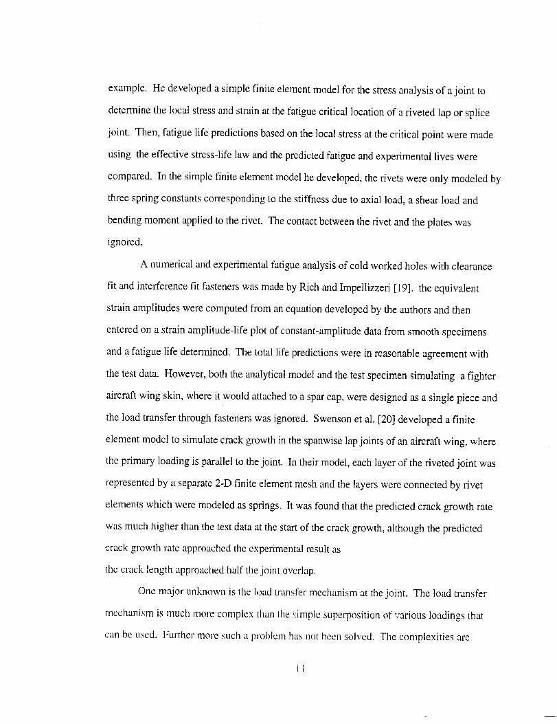
example.Hedevelopedasimplefiniteelementmodelfor thestressanalysisof ajoint to
determinethelocalstressandstrainatthefatiguecriticallocationof arivetedlapor splice
joint. Then,fatiguelife predictionsbasedonthelocalstressatthecriticalpointweremade
using theeffectivestress-lifelawandthepredictedfatigueandexperimentalliveswere
compared.In thesimplefiniteelementmodelhedeveloped,therivetswereonlymodeledby
threespringconstantscorrespondingto thestiffnessdueto axial load,a shearloadand
bendingmomentappliedto therivet. Thecontactbetweentherivetandtheplateswas
ignored.
A numericalandexperimentalfatigueanalysisof coldworkedholeswith clearance
fit andinterferencefit fastenerswasmadebyRichandImpellizzeri[19]. theequivalent
strainamplitudeswerecomputedfromanequationdevelopedbytheauthorsandthen
enteredonastrainamplitude-lifeplotof constant-amplitudedatafromsmoothspecimens
andafatiguelife determined.Thetotallifepredictionswerein reasonableagreementwith
thetestdata.However,boththeanalyticalmodelandthetestspecimensimulatingafighter
aircraftwingskin,whereit wouldattachedto asparcap,weredesignedasasinglepieceand
theloadtransferthroughfastenerswasignored.Swensonetal. [20] developedafinite
elementmodelto simulatecrackgrowthin thespanwiselapjoints of anaircraftwing, where
theprimaryloadingisparalleltothejoint. In theirmodel,eachlayerof therivetedjoint was
representedby aseparate2-D finiteelementmeshandthelayerswereconnectedby rivet
elementswhichweremodeledassprings.It wasfoundthatthepredictedcrackgrowthrate
wasmuchhigherthanthetestdataatthestartof thecrackgrowth,althoughthepredicted
crackgrowthrateapproachedtheexperimentalresultas
thecracklengthapproachedhalf thejoint overlap.
Onemajorunknownis the loadtransfermechanismatthejoint. Theloadtransfer
mechanismis muchmorecomplexthanthesimplesuperpositionof variousloadingsthat
canbeused.Further more such a problem has not been solved. The complexities are
il
surface-to-surfacecontactbetweentherivetandtheplates,thejoint rotationdueto non-
axialityof loadingandnonsymmetryof theconfiguration,andrivetclamp-upand
interference.Becausetheproblemis 3-D,thecomplexityis increasedby oneorderof
magnitude.Furthermore,thecontactdeformationisnonlinear,hencerequiresthesolution
of avariableBVP (boundaryvalueproblem).Analysisof rivetedjoints includingthese
factorsis importantfor theefficientdesignofjoints, establishingthetruefactorof safety,
andto verify theadequacyof thepresentdesignguidelines.
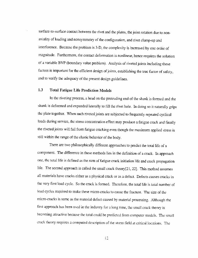
1.3 Total Fatigue Life Prediction Models
In the riveting process, a head on the protruding end of the shank is formed and the
shank is deformed and expanded laterally to fill the rivet hole. In doing so it naturally grips
the plate together. When such riveted joints are subjected to frequently repeated cyclical
loads during service, the stress concentration effect may produce a fatigue crack and finally
the riveted joints will fail from fatigue cracking even though the maximum applied stress is
still within the range of the elastic behavior of the body.
There are two philosophically different approaches to predict the total life of a
component. The difference in these methods lies in the definition of a crack. In approach
one, the total life is defined as the sum of fatigue crack initiation life and crack propagation
life. The second approach is called the small crack theory[21, 22]. This method assumes
all materials have cracks either as a physical crack or as a defect. Defects causes cracks in
the very first load cycle. So the crack is formed. Therefore, the total life is total number of
load cycles required to make these micro-cracks to cause the fracture. The size of the
micro-cracks is same as the material defect caused by material processing. Although the
first approach has been used in the industry for a long time, the small crack theory is
becoming attractive because the total could be predicted from computer models. The srnall
crack theory requires a computed description of the stress field at critical locations. The
12

crackgrowthiscalculatedunderthosestressfield. Themicro-crackpropagationis
calculatedunderthe influenceof stressconcentration.Whenthecrackbecomesone-tenth
of amillimeter,thecompletestressfield will beusedfor crackpropagation.Therefore,
stressanalysisof ajoint includingall joint complexitiesiscriticalto successfulpredictionof
thetotal life of thejoint usingsmallcracktheory.
1.4 Rivet Clampup and Interference
The riveting process consists of inserting the rivet in matching holes of the pieces to
be joined and subsequently forming a head on the protruding end of the shank, the holes
are generally 1/16 in. greater than the nominal diameter of undriven rivet. The head is
formed by rapid forging with a pneumatic hammer or by continuous squeezing with a
pressure riveter. The latter process is confined to use in shop practice, whereas pneumatic
hammers are used in both shop and field riveting. In addition to forming the head, the
diameter of the rivet is increased, resulting in a decreased hole clearance or the expansion of
the hole (interference) [23].
Most rivets are installed as hot rivets, but some shop rivets are driven cold. Both
processes introduces clampup force and interference to the joint.
During the riveting process the enclosed plies are drawn together with installation
bolts and by the rivet equipment. As the rivet cools, it shrinks and squeezes the connected
plies together. A residual clamping force or internal tension results in the rivet. The
magnitude of the residual clamping force depends on the joint stiffness, critical installation
conditions such as driving and finishing temperature, as well as driving pressure.
Measurements have shown that hot driven rivets can develop clamping forces that approach
the yield load of the rivet. Residual clamping forces are also observed in cold driven rivets.
This results mainly from the elastic recovery, of the gripped plies after the riveter, which
squeezed the plies together during the riveting process, is removed. Generally, the clamping
13
forceincold-formedrivetsissmallwhencomparedwith theclampingforce insimilarhot-
drivenrivets. Theclampingforcein therivet isdifficult to control,howeverarangeof
clampupforceasapercentageof therivetyield loadcanbeassumedfor analysis.
Thecriticaljoint componentin a lapjoint subjectedtorepeatedloadingisnot the
fastenerbut theplatematerial.A severedecreasein theplatefatiguestrengthis apparentin
unrestrainedlapjoints. Theinherentbendingdeformationscauselargestressrangesto
occurat thediscontinuitiesof thejoint. Thebendingstresscombineswith thenormal
stressandresultsin high localstressesthatreducethefatiguestrengthof the lapjoint.
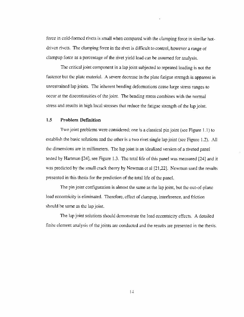
1.5 Problem Definition
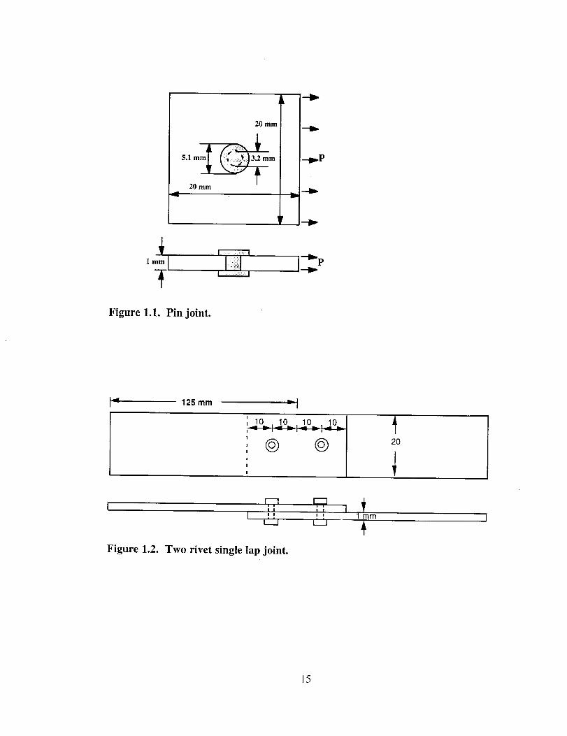
Two joint problems were considered; one is a classical pin joint (see Figure 1. I) to
establish the basic solutions and the other is a two rivet single lap joint (see Figure 1.2). All
the dimensions are in millimeters. The lap joint is an idealized version of a riveted panel
tested by Hartman [24], see Figure 1.3. The total life of this panel was measured [24] and it
was predicted by the small crack theory by Newman et al [21,22]. Newman used the results
presented in this thesis for the prediction of the total life of the panel.
The pin joint configuration is almost the same as the lap joint, but the out-of-plane
load eccentricity is eliminated. Therefore, effect of clampup, interference, and friction
should be same as the lap joint.
The lap joint solutions should demonstrate the load eccentricity effects. A detailed
finite element analysis of the joints are conducted and the results are presented in the thesis.
I"4-
5.1 mm
'r
20 mm
20 mm
--._P
lmm[
Figure 1.1. Pin joint.
125 turn -I
!
I
: @ @!
I
I
2O
! iI " II I lm m
,", ,'_.u _.
Figure 1.2. Two rivet single lap joint.
15
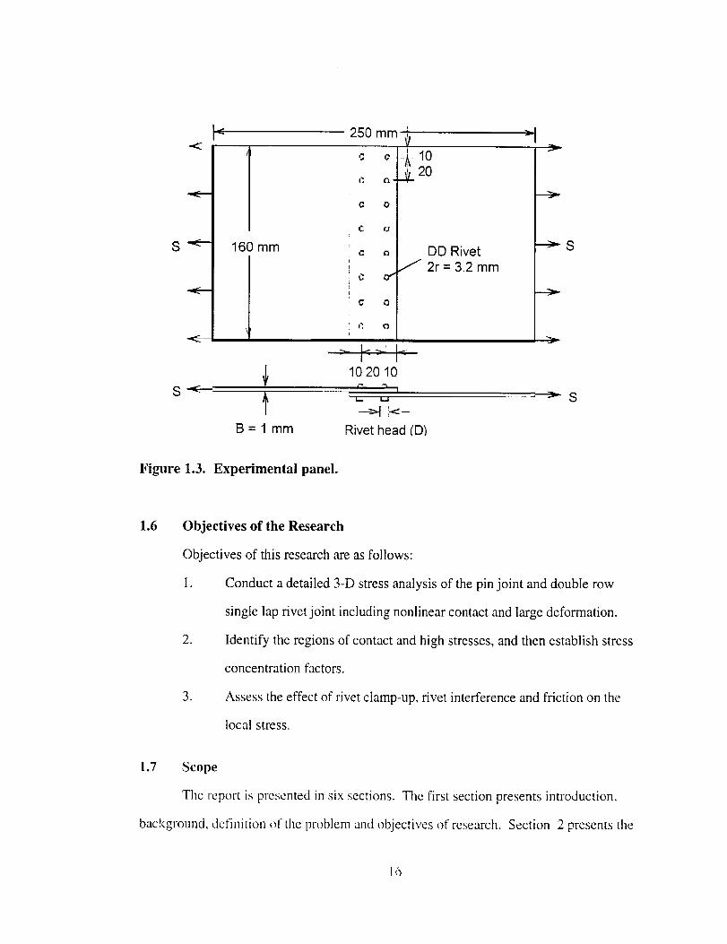
,,<---.-
S
S
160 mm
l
250 m m..._., 7-klO,- _. _g. 20
DD Rivet/ 2r = 3.2 mm
10 20 10
I
B=lmm
-->t .._-
Rivet head (D)
--_S
>S
Figure 1.3. Experimental panel.
1.6 Objectives of the Research
Objectives of this research are as follows:
1. Conduct a detailed 3-D stress analysis of the pin joint and double row
single lap rivet joint including nonlinear contact and large deformation.
2. Identify the regions of contact and high stresses, and then establish stress
concentration factors.
3. Assess the effect of rivet clamp-up, rivet interference and friction on the
local stress.
1.7 Scope
The report is presented in six sections. Tile first section presents introduction,
background, definition or the problem and objectives of research. Section 2 presents the
16
description of finite element modeling of the two joints and modeling rivet clampup and
interference effect. Also discussed in this section is the convergence criteria used for the
non-linear analysis. Section 3 details the pin joint analysis for the neat fit, friction, clampup,
interference and the combined case. The combined case is a combination of the rivet
clampup, interference and friction. Section 4 covers the two rivet single lap joint analysis.
In section 5 the neat fit case has been extended to elastic - plastic analysis to simulate a
more realistic condition and the local stresses in the two rivet joint. Conclusions from the
study are summarized in section 6..
_7

2. FINITE ELEMENT MODELING OF RIVETED JOINT
2.1 Introduction
This section describes the finite element modeling of the rivet joint, contact, friction,
clampup and interference. The general analysis procedure and convergence criteria
are presented.
2.2 Finite Element Analysis
A stress analysis problem involves the differential equations of equilibrium and
compatibility, together with the stress strain relationships and the boundary conditions.
Analytical solutions to real life problems are seldom possible, and it is necessary, therefore,
to employ a numerical method.
A number of numerical stress analysis techniques are currently available, and their
implementation is being greatly facilitated by the increasingly widespread availability of
computers. The essential common feature of these methods is that the original problem,
posed in terms of differential equations in the unknown continuous functions, is replaced by
a formulation involving a set of algebraic equations in the discrete values of the unknowns at
a finite number of points in the solid. In other words, the continuum model of the problem
is approximated by a discrete model having a finite number of degrees of freedom.
Of the numerical methods available the finite element method is the most widely
used. The finite element method is a numerical procedure for obtaining solutions to many
of the problems encountered in engineering analysis. It is impossible to document the exact
origin of the finite element method because the basic concepts have evolved over a period of
150 or more years. The inethod as we know it today is an outgrowth of several papers
published in the 1950s that extended the matrix analysis of :structures to continuum bodies.
The space exploration of the 1960s provided money for basic reseamh, which placed tile
18

method on a firm mathematical foundation and stimulated the development of multiple-
purpose computer programs that implemented the method. The design of airplanes,
missiles, space vehicles, and the like, provided application areas. Although the origin of the
method is vague, its advantages are clear. The method is easily applied to irregular shaped
objects composed of several different materials and having mixed boundary conditions. It
is applicable to steady-state and time dependent problems as well as problems involving
both geometric and material nonlinearity.
The finite element method combines several mathematical concepts to produce a
system of linear or nonlinear equations. The number of equations is usually very large,
running to several thousand depending on the problem that is being solved, and requires the
computational power of the computer. The method has little practical value if modem
computers are not available. The basis of the method is the representation of a structure by
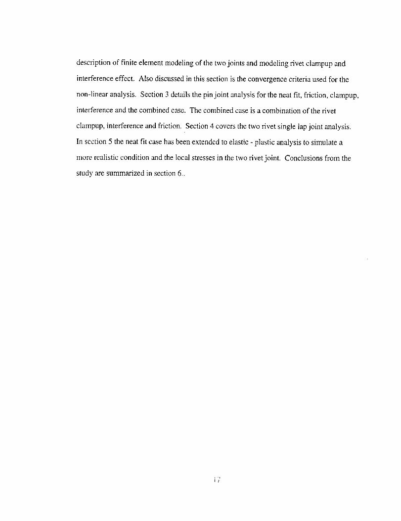
an assemblage of subdivisions or finite elements as shown in Figure 2.1. These finite
elements are considered to be connected at joints, called nodes or nodal points, at which the
values of the unknowns (usually the displacements) are to be approximated. Successive
finer discretization of the structure would lead to the exact solution. Therefore, it is likely
that a moderately fine subdivision will provide a solution of acceptable accuracy. The
computational effort required to obtain a solution will depend upon the number of degrees
of freedom in the finite element model. In engineering practice a limit will be imposed on
the degree of subdivision of the structure by the need to strike a balance between computing
costs and solution accuracy.
19
Nodalpoint Element
Figure 2.1. Representation of a two-dimensional solid as an assemblage oftriangular finite elements.
Numerous commercial finite element analysis software packages are now available
for simulating and solving complex engineering problems. One such code is ANSYS [25].
One of the advantage of ANSYS is its capability for geometric modeling and post-
processing. Geometric modeling, analysis and results visualizations are all in the package.
The analysis options include static, dynamic, material and geometric nonlinear analysis. In
addition to having standard l-D, 2-D, 3-D elements, it has line to line and surface to surface
contact elements. These elements are needed for the present analysis of riveted
joint.
2.3 Finite Element Modeling of Rivet Joint
The finite element model of the rivet joint (refer to Figure 1.I and 1.2) consists of
three main components nameIy the top plate, bottom plate and the rivet.
The plates and rivet are discretized using the SOLID45 3-D 8-Node Structural Solid
element. The element is defined by 8 nodes having three degrees of freedom per node
(translations in the nodal x, y, and z directions). The element may have any spatial
orientation. The element has plasticity, stress stiffening, large deflection, and large strain
capabilities.
element has
boundaries.
It can tolerate irregular shapes without much loss of accuracy. SOLID45
compatible displacement shapes and are well .uited to model curved
2O
Contactoccursbetweenthetopplateandthebottomplate,therivetandtheplate
holes,therivet headandtheplate. In theANSYSprogramgeneralcontactis aboundary
nonlinearityfeaturethatpermitssurface-to-surfacecontactanalysiswith largedeformations,
contactandseparation,coulombfrictionsliding,andheattransfer.Generalcontactis
representedin theANSYSprogramby followingthepositionof pointson onesurface(the
contactsurface)relativetolinesor areasof anothersurface(thetargetsurface).The
programusescontactelementsto tracktherelativepositionsof thetwo surfaces.Contact
elementsaretriangles,tetrahedronorpyramids,wherethebaseismadeup of nodesfrom
thesecondsurface(thetargetsurface)andtheremainingvertexisanodefrom the 1st
surface,thecontactsurface.An analysisthatincorporatesgeneralcontactsurfacescan
easilyrequiretheuseof hundredsor eventhousandsof contactelements.Fortunately,
specialfeatureshavebeenincludedin theANSYSprogramto makegeneratingandusing
theseelementsasefficientaspossible.Duringsolution,theprogramidentifiesthose
relativelyfewcontactelementsthatareexpectedtoaffectthesolution(i.e.thoseapproaching
contactor incontact).Theremainingelementsaretemporarilyignored,producingnull
elementstiffnessmatrices.As aresult,anincreasein thenumberof contactelementsthat
arenot in contactwill notdegraderuntimesasseverelyaswouldasimilar increase
involvingotherelementtypes.Thecontactelementusedfor thepresentproblemis
CONTAC493-DPointto SurfaceContact.
2.3.1 CONTAC49 Element Description
CONTAC49 is a 5 node element that is intended for general contact analysis. In a
general contact analysis, the area of contact between two or more bodies is generally not
known in advance. In addition the finite element models of the contacting bodies are
generated in such a way that precise node-to-node contact is neither achievable nor desirable
when contact is established. The CONTAC49 element has the capability to represent
21
general contact of models that are generated with arbitrary meshes. In other words, its use
is not limited to known contact or node-to-node configurations.
CONTAC49 is applicable to 3-D geometry. It may be applied to the contact of
solid bodies or shells, to static or dynamic analyses, to problems with or without friction,
and to flexible-to-flexible or rigid-to-flexible body contact.
Contact Kinematics
Contact kinematics is concerned with the precise tracking of contact nodes and
surfaces in order to define clear and unambiguous contact conditions. The primary aim is
to delineate between open (i.e., not in contact) and closed (in contact) contact situations.
This task is accomplished by various algorithms embedded in the CONTAC49 element.
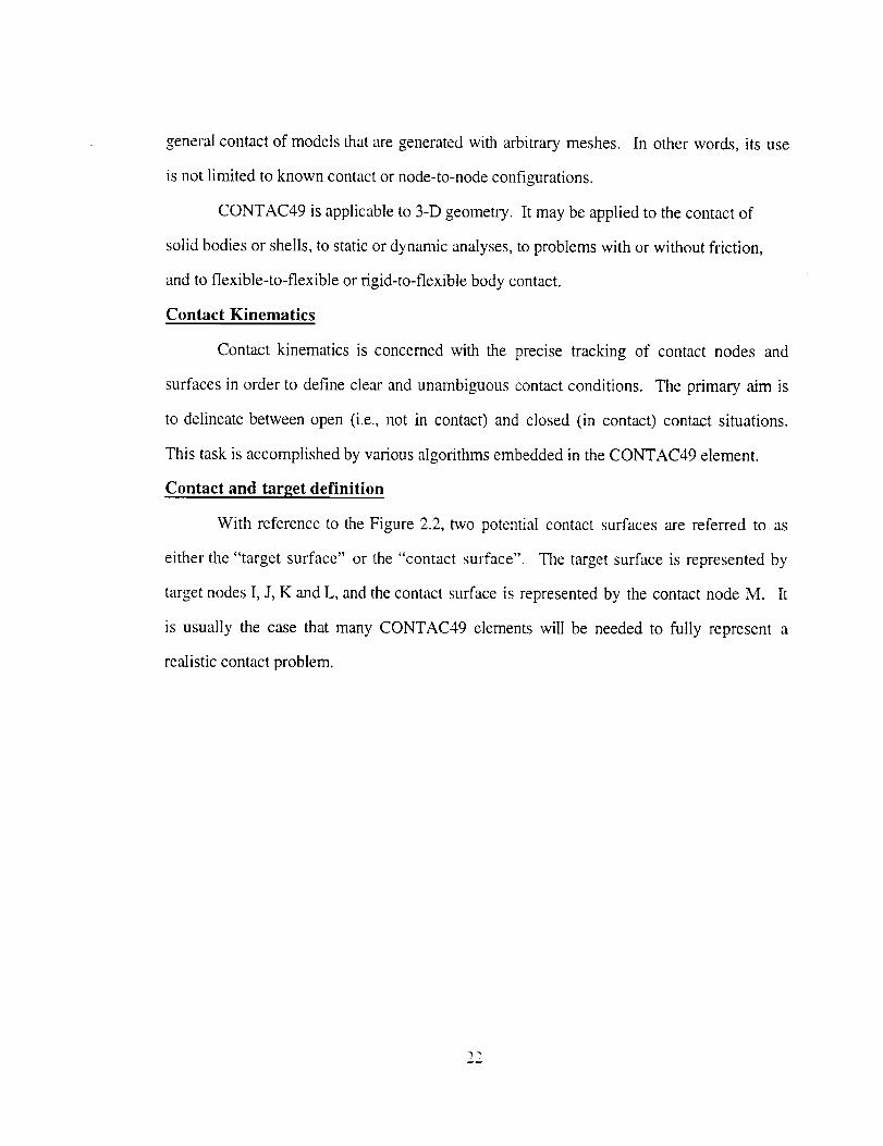
Contact and target definition
With reference to the Figure 2.2, two potential contact surfaces are referred to as
either the "target surface" or the "contact surface". The target surface is represented by
target nodes I, J, K and L, and the contact surface is represented by the contact node M. It
is usually the case that many CONTAC49 elements will be needed to fully represent a
realistic contact problem.
m_
Contact Surfaces and Nodes
M
Target Surfaces andNodes
Figure 2.2. The CONTAC49 element configuration.
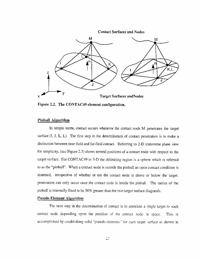
Pinball Algorithm
In simple terms, contact occurs whenever the contact node M penetrates the target
surface (I, J, K, L). The first step in the determination of contact penetration is to make a
distinction between near-field and far-field contact. Referring to 2-D transverse plane view
for simplicity, (see Figure 2.3) shows several positions of a contact node with respect to the
target surface. For CONTAC49 in 3-D the delimiting region is a sphere which is referred
to as the "pinball". When a contact node is outside the pinball an open contact condition is
assumed, irrespective of whether or not the contact node is above or below the target.
penetration can only occur once the contact node is inside the pinball. The radius of the
pinball is internally fixed to be 50% greater than the two target surface diagonals.
Pseudo Element Algorithm
The next step in the determination of contact is to associate a _ingle target to each
contact node depending upon the position of the contact node in space. This is
accomplished by establishing solid "pseudo elements" for each target _urface as shown in
N_
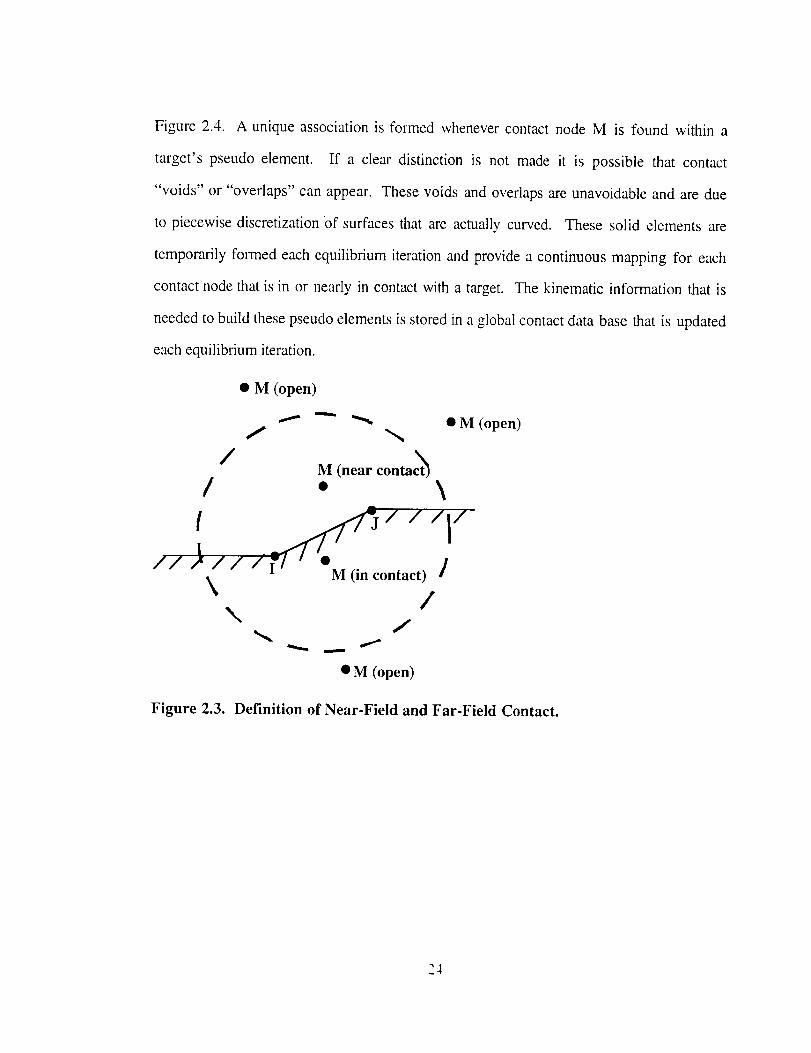
Figure 2.4. A unique association is formed whenever contact node M is found within a
target's pseudo element. If a clear distinction is not made it is possible that contact
"voids" or "overlaps" can appear. These voids and overlaps are unavoidable and are due
to piecewise discretization Of surfaces that are actually curved. These solid elements are
temporarily formed each equilibrium iteration and provide a continuous mapping for each
contact node that is in or nearly in contact with a target. The kinematic information that is
needed to build these pseudo elements is stored in a global contact data base that is updated
each equilibrium iteration.
• M (open)
/M (near contac_
/ • X
• M (open)
!II i l I I irl ' %,,. /
M (in contact)
\ /"- /
• M (open)
Figure 2.3. Definition of Near-Field and Far-Field Contact.
24
L 3"
Figure 2.4. Pseudo Element.
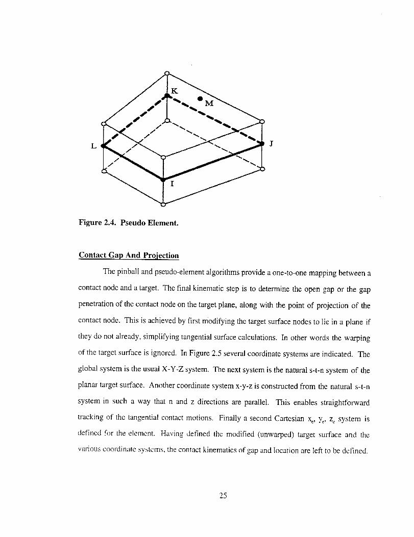
Contact Gap And Prq[ection
The pinball and pseudo-element algorithms provide a one-to-one mapping between a
contact node and a target. The final kinematic step is to determine the open gap or the gap
penetration of the contact node on the target plane, along with the point of projection of the
contact node. This is achieved by first modifying the target surface nodes to lie in a plane if
they do not already, simplifying tangential surface calculations. In other words the warping
of the target surface is ignored. In Figure 2.5 several coordinate systems are indicated. The
global system is the usual X-Y-Z system. The next system is the natural s-t-n system of the
planar target surface. Another coordinate system x-y-z is constructed from the natural s-t-n
system in such a way that n and z directions are parallel. This enables straightforward
tracking of the tangential contact motions. Finally a second Cartesian xo, y_, zc system is
defined for the element. Having defined the modified (unwarped) target surface and the
various coordinate systems, the contact kinematics of gap and location are left to be defined.
25
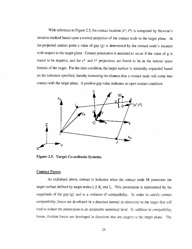
With referencetoFigure2.5,thecontactlocation(s*, t*) is computedby Newton's
iterativemethodbaseduponanormalprojectionof thecontactnodeto thetargetplane. At
theprojectedcontactpoint a valueof gap(g) is determinedby thecontactnode's location
with respectto thetargetplane.Contactpenetrationisassumedto occurif thevalueof g is
found to be negative,andthes* and t* projectionsare found to be in the naturalspace
boundsof thetarget.For thelatercondition,thetargetsurfaceis internallyexpandedbased
on thetolerancespecified,therebyincreasingthechancesthat a contactnodewill comeinto
contactwith thetargetplane.A positivegapvalueindicatesanopencontactcondition.
n
Ze _ #t Mo (s',t*)
i Ij_ " x /S:e
Figure 2.5. Target Co-ordinate Systems.
Contact Forces
As explained above, contact is indicated when the contact node M penetrates the
target surface defined by target nodes I, J, K, and L. This penetration is represented by the
magnitude of the gap (g) and is a violation of compatibility. In order to satisfy contact
compatibiIity, tbrces are developed in a direction normal (n-direction) to the target that will
tend to reduce the penetration to an acceptable numerical level. In addition to compatibility
forces, tYiction forces ate developed in directions that are tangent to the target plane. The
26
normal and tangential friction forces that are described here are referenced to the local x-y-z
system shown in Figure 2.5.
Normal forces
Two methods of satisfying contact compatibility are available for CONTAC49: a
penalty method and combined penalty plus lagrange multiplier method. The penalty method
approximately enforces compatibility by means of a contact stiffness (i.e., the penalty
parameter). The combined approach satisfies compatibility to a user defined precision by
the generation of additional contact forces (i.e., Lagrange forces).
For the penalty method,
f, ={0Kng ifg<0if g>0
where K, is the contact stiffness (real constant KN).
For the combined method, the Lagrange multiplier component of force is computed
locally (for each element) and iteratively. It is expressed as
f, = min (0. K,g + A,i+I)
Where : ,71,_+_= Lagrange multiplier force at iteration i + 1
= _X_ + aK.g if [gl > e
tZi if Igl< e
e = user- defined compatibility tolerance (Input quantity TOLN
on R command
= an internally computed factor (a < 1)
Friction forces
The CONTAC49 element considers three friction models: frictionless, elastic
coulomb friction, and rigid coulomb friction. The Coulomb friction representations require
27
theinput of thecoefficientof sliding friction (g). Frictioncausesthetangentialforces,as
thecontactnodesmeetsandmovesalongthetargetsurface.
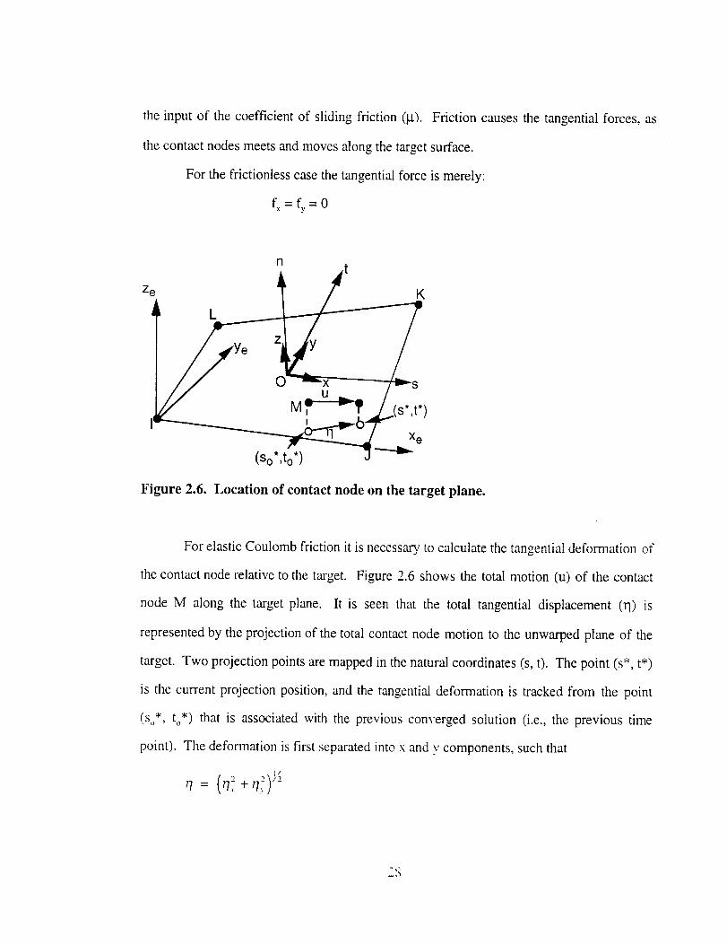
Forthefrictionlesscasethetangentialforceis merely:
fx=f,=0
rlt
Z e
l(So*,to*)
Figure 2.6. Location of contact node on the target plane.
For elastic Coulomb friction it is necessary to calculate the tangential deformation of
the contact node relative to the target. Figure 2.6 shows the total motion (u) of the contact
node M along the target plane. It is seen that the total tangential displacement (1"1) is
represented by the projection of the total contact node motion to the unwarped plane of the
target. Two projection points are mapped in the natural coordinates (s, t). The point (s*, t*)
is the current projection position, and the tangential deformation is tracked from the point
(so*, to* ) that is associated with the previous converged solution (i.e., the previous time
point). The deformation is first separated into x and y components, such that
= +

where: qx = component of rl in the local x direction
fly = component of q in the local y direction
Next, the deformation is decomposed into elastic (or sticking) and sliding (or inelastic)
components.
rT,= _ + 77;e
fir = T_), "t- T_, s,.
Related tangential forces are:
L = X,<ff
f,. = K,,7,,
where: K, = sticking stiffness
It follows that the magnitude of the tangential forces is
s.,.= +
The stiffness and the load vector for the CONTAC49 element is given below
{N}r=[0 0 q, 00q2 00 q3 00q4 00 1]
{N_}r=[q, 0 0 q2 0 0 q3 0 0 q4 0 0 1 0 O]
{Ny}r=[0 q, 00q2 00q3 00q4 001 01
For the 4- node target, individual interpolates are
I(1- s_q, =--_ )(1- t*)
q2=-l(l+s*)( l-t'),,
=-1(1 + s')(l +t*)q3
+c)
In the normal direction, the force applied to the contact node (M) is balanced by opposite
forces applied to the target nodes; that is,
29
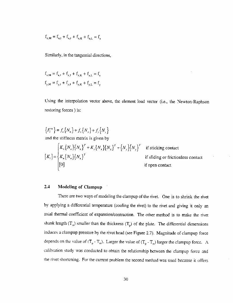
f.,.-- f.,,+ f.,j÷ fn,K+ f.,L----f.
Similarly, in the tangential directions,
f.,. = fx,,+ fxj+ fx,K+ fx,L= f.
f,,. = f,, + f,, + f,,K+ fy,L= fy
Using the interpolation vector above, the element load vector (i.e., the Newton-Raphson
restoring forces ) is:
{F:°}-- I,,{N,,}+ {Nx}+Z{N,}and the stiffness matrix is given by
if sticking contact
if sliding or frictionless contact
if open contact
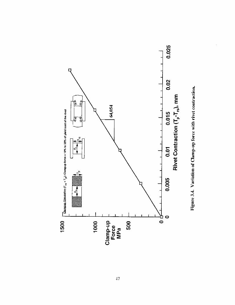
2.4 Modeling of Clampup
There are two ways of modeling the clampup of the rivet. One is to shrink the rivet
by applying a differential temperature (cooling the rivet) to the rivet and giving it only an
axial thermal coefficient of expansion/contraction. The other method is to make the rivet
shank length (Trs) smaller than the thickness (Tp) of the plate. The differential dimensions
induces a clampup pressure by the rivet head (see Figure 2.7). Magnitude of clampup force
depends on the value of (Tp - Trs). Larger the value of (Tp - Trs) larger the clampup force. A
calibration study was conducted to obtain the relationship between the clampup force and
tile rivet shortening. For the current probIem the second method was used because it offers
3O
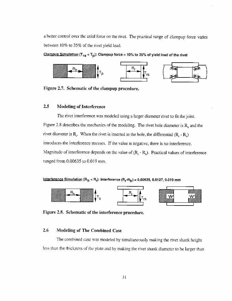
a better control over the axial force on the rivet. The practical range of clampup force varies
between 10% to 35% of the rivet yield load.
Clamoup Simulation (Trs < Tp): Clampup force = 10% to 35% of yield load of the rivet
iT0I
Figure 2.7. Schematic of the clampup procedure.
2.5 Modeling of Interference
The rivet interference was modeled using a larger diameter rivet to fit the joint.
Figure 2.8 describes the mechanics of the modeling. The rivet hole diameter is R h and the
rivet diameter is R r. When the rivet is inserted in the hole, the differential (R_ - R,)
introduces the interference stresses. If the value is negative, there is no interference.
Magnitude of interference depends on the value of (R r - Rh). Practical values of interference
ranged from 0.00635 to 0.019 ram.
Interference Simulation (R h < Rr): Interference (Rr-Rh) = 0.00635, 0.0127, 0.019 mm
iToI I
Figure 2.8. Schematic of the interference procedure.
2.6 Modeling of The Combined Case
The combined case was modeled by simultaneously making the rivet shank height
less than the thickness of the plate and by making the rivet shank diameter to be larger than
31

the plate hole diameter.
2.7 Analysis Procedure
The commercial finite element code 'ANSYS' was used. The displacement method
of analysis was used. The linear solution was obtained by the frontal solver. Before
solution, ANSYS automatically reorders the elements for a smaller wavefront (smaller the
wavefront less the CPU time required for solution). The nonlinear solutions are obtained
from the Newton-Raphson iterative algorithm. The analysis was conducted by incrementing
the displacement and calculating the equilibrium condition and the associated stress-strain
field. The analysis was continued till desired stress state or the loading was
attained.
2.8 Convergence Criteria
The force convergence criteria was used to solve the problem. This is the most
efficient convergence criteria for nonlinear finite element problems. Since both nonlinear
geometry and changing status elements were used in the model the convergence criteria was
slackened to avoid convergence difficulties. The convergence criteria was arrived at in an
iterative manner, slackening the convergence criteria whenever convergence problems were
encountered.
The finite element discretization process yields a set of simultaneous equations:
[x]{.}: {Fa}
where:
[x]
{.}
{F"}
= coefficient matrix
= vector of unknown degree of freedom values
= vector of applied loads
32

If thecoefficientmatrix is itselfafunctionof theunknownDOFvalues(or theirderivatives)
thentheaboveequationisnonlinear.TheNewton-Raphsonmethodisaniterativeprocess
of solvingthenonlinearequationsandcanbewrittenas:
K T = -[ i ]{Aui} {F"} {Fi ''r}
where:
i
{F:r}
= Jacobian matrix (tangent matrix)
= subscript representing the current equilibrium iteration
= vector of restoring loads corresponding to the element internal loads.
{ F" } - {F, "r } = residual or out of balance load vector.
In a structural analysis, [KIT] is the tangent stiffness matrix, {u i} is the
displacement vector and {F_"r } is the restoring force vector calculated from element
stresses.
The iteration process described continues untiI convergence is achieved.
Convergence is assumed when:
II{R}II<
where {R} is the residual vector;
{R}={F"}-{F, "r}
H{R}II--(Z (Euclidean norm)
e n = tolerance value
Convergence, therefore, is obtained when size of the residual (disequilibrium) is less
than a tolerance times a reference value. The default out of balance reference value
3.3
IIr 'll,
2.9 Summary
With the advent of modem day computers and their ability to crunch numbers, finite
element analysis has gained favor in the industry as an essential tool in their design process.
ANSYS finite element code was used in this research project. The main reason being its
capability to simulate contact between two bodies and its capability to do nonlinear analysis.
Also a method of introducing rivet clampup and interference to the rivet joint was developed.
34
3. PIN JOINT ANALYSIS
3.1 Introduction
In this section a classical pin joint was modeled using 3-D finite elements. This
joint is loaded by remote tension and is restrained by a pin. The effects of clampup and
interference on the stress distribution in the hole boundary is presented in this section.
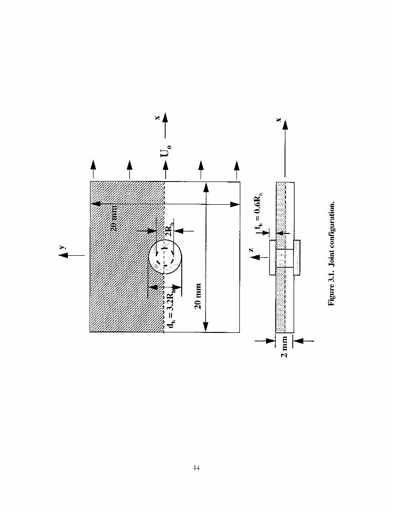
3.2 Joint Configuration
Figure 3.1 shows the geometry i.e. configuration of the pin joint. The plate was
square with the edge being 20 mm and thickness being 2 ram. The hole was located in the
center of the plate with a radius R h of 1.6 ram. The pin head had a diameter (d h = 3.2R h)of
5.1 rnm and thickness of 1.0 mm (0.6Rh). The radius to width and radius to edge distance
is greater than 6, hence the joint configuration represents the infinite plate configuration.
The global Cartesian coordinate system is represented by x, y, z. The pin is fixed at its
center line and the plate is pulled by a uniform displacement Uo in the x direction. The pin
bearing load (P) is the integral of x- directional reaction at the edge x = 10 mm. The
geometry and the loading are symmetric about y = 0 and z = 0 planes. Hence, only one-
quarter of the joint (shown by the shaded region) was modeled by finite elements.
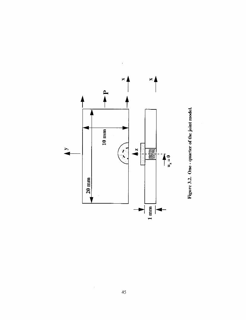
3.3 Analysis Model
The joint symmetry was exploited to reduce computational time. Figure 3.2 shows
the one - quarter geometry of the joint. The plate was loaded at x = I0 mm with a uniform
displacement u x and the axis of the pin was fixed in the x and y direction (that is u_ = u v = 0
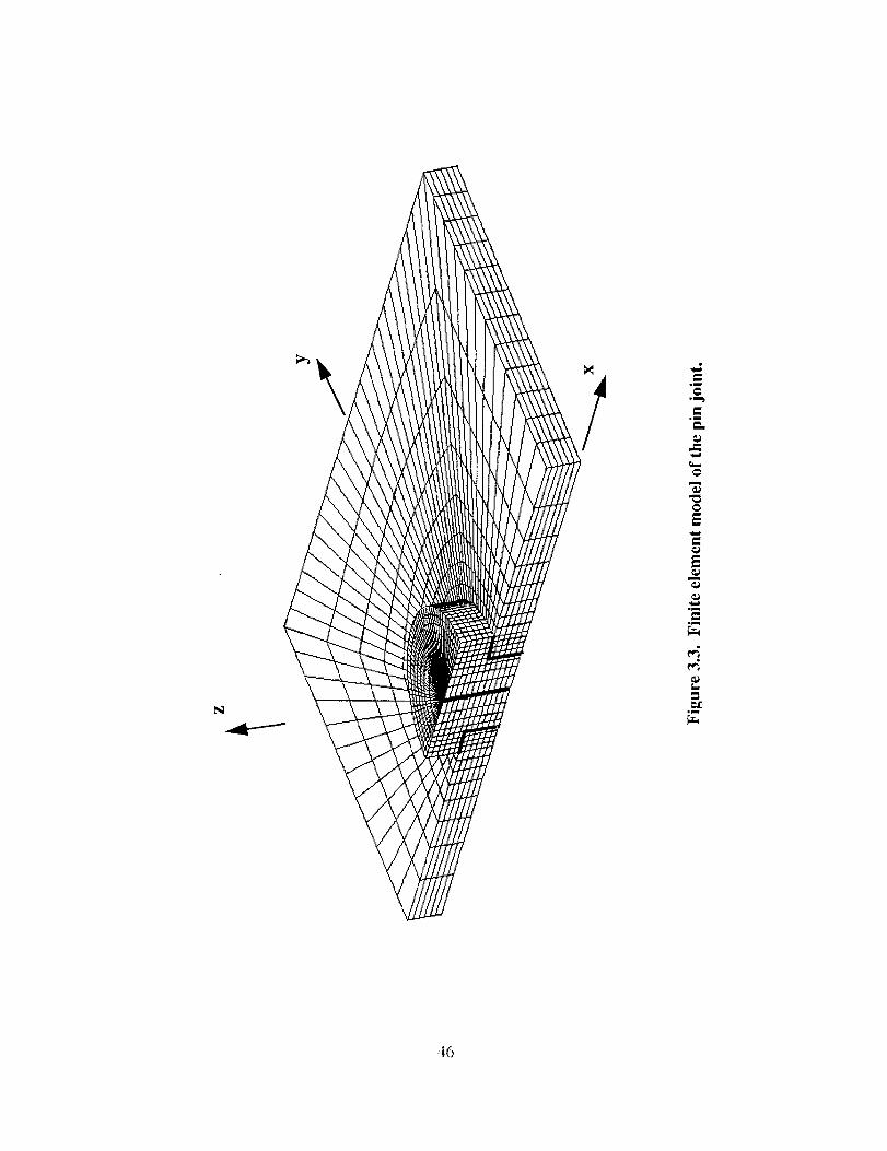
for the axis of the pin). The plate and the pin was modeled using 8-noded brick elements,
SOLID45 in the ANSYS code. The 3-D surface to surface contact elements were used to
simulate contact between the pin and the plate hole and pinhead and the plate surface. The
finite elementmodelhad6912SOLID45elements(3456elementseachin plateandpin)
and i920 CONTAC49elements.Figure3.3showsthefinite elementmesh.
Theotherboundaryconditionsimposedon themodelwereu,,= 0 ony = 0 plane
anduz= 0 onz = 0 plane.Thesetwoboundaryconditionssimulatesymmetricdeformation
of thejoint.
3.4 Analysis Cases
Therearetwo typesof non-linearitiesthatareexpectedin themodel,viz.,nonlinear
contactboundaryandlargerotation.Therefore,largedeformationandnon-linearcontact
strategiesareusedin theanalysis.A commercialcodeANSYS5.3 was used. The non-
linearities were solved by a modified Newton-Raphson iteration algorithm. The Lagrange
multiplier and penalty methods are used for contact modeling. The defined maximum
gap/penetrations and contact stiffnesses are 0.01Hs and 2000 N/ram: _about 3% of the
elastic modulus of the plate material, which was within the recommended range)
respectively. The parameter Hs is the smallest element size in the model, which was 1/6
mm. The residual force convergence criteria was used at every node to establish the
convergence of the non-linear solution. The relative error in the nodal residual forces was
less than 0.1% of total applied force as a convergence criteria.
The analysis was conducted for four different cases that occur in the joint: neatfit,
clampup, friction and interference, and a selected combined case. The neatfit represents the
baseline solution. This case represents no surface - surface friction, no clampup and no
interference. Analytical modeling of each of these parameters are explained in section 2 and
is summarized in the following sections. The analysis was conducted by incrementally
loading the joint to an applied remote stress of about 150 MPa or about U o = 0.1 mm.
3O
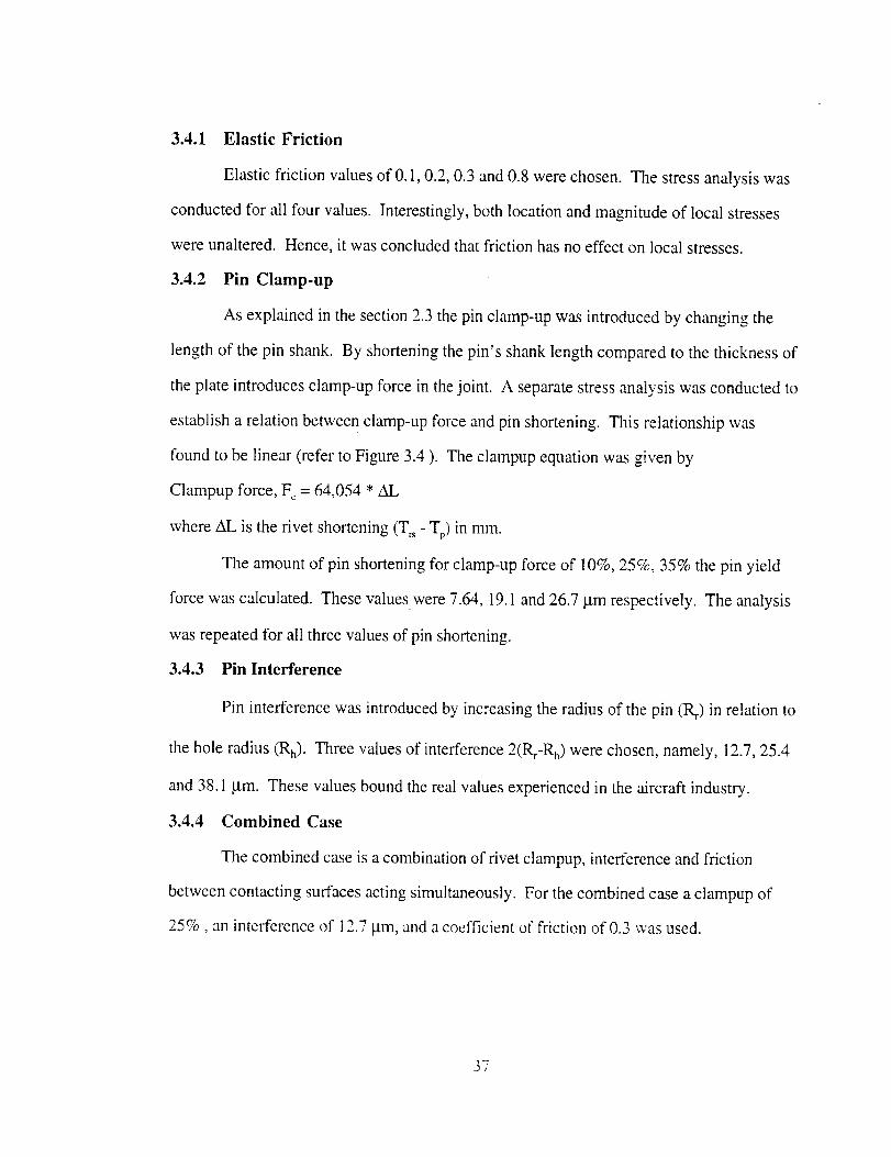
3.4.1 Elastic Friction
Elastic friction values of 0.1, 0.2, 0.3 and 0.8 were chosen. The stress analysis was
conducted for all four values. Interestingly, both location and magnitude of local stresses
were unaltered. Hence, it was concluded that friction has no effect on local stresses.
3.4.2 Pin Clamp-up
As explained in the section 2.3 the pin clamp-up was introduced by changing the
length of the pin shank. By shortening the pin's shank length compared to the thickness of
the plate introduces clamp-up force in the joint. A separate stress analysis was conducted to
establish a relation between clamp-up force and pin shortening. This relationship was
found to be linear (refer to Figure 3.4 ). The clampup equation was given by
Clampup force, F c = 64,054 * AL
where AL is the rivet shortening (Trs - To) in mm.
The amount of pin shortening for clamp-up force of 10%, 25%, 35% the pin yield
force was calculated. These values were 7.64, 19.1 and 26.7 _tm respectively. The analysis
was repeated for all three values of pin shortening.
3.4.3 Pin Interference
Pin interference was introduced by increasing the radius of the pin (R 0 in relation to
the hole radius (Rh). Three values of interference 2(t_-Rh) were chosen, namely, 12.7, 25.4
and 38.1 lain. These values bound the real values experienced in the aircraft industry.
3.4.4 Combined Case
The combined case is a combination of rivet clampup, interference and friction
between contacting surfaces acting simultaneously. For the combined case a clampup of
25%, an interference of 12.7 _tm, and a coefficient of friction of 0.3 was used.
37

3.5 Results
Resultsof theanalysisconductedfor variouscasesarerepresentedin thefollowing
subsections.First,neatfit (zerosurface-surfacefriction) resultsarepresented.Thenthe
effectsof clamp-upandinterferenceon localstressesareexamined.Theprimaryfocuswas
on themaximumhoopstressontheholeboundaryandthehoopstressat90°to thez-axis.
The2ndcaserepresentslocationof maximumhoopstressfor openholeproblems.All
localstressesarenormalizedbytheremotestress(_,) asmuchaspossible.Theremote
stresswascalculatedbydividingthetotalreactionatx = 10mm edgebytheareaof cross-
section( 10xl mm2).
3.5.1 Neat Fit Results
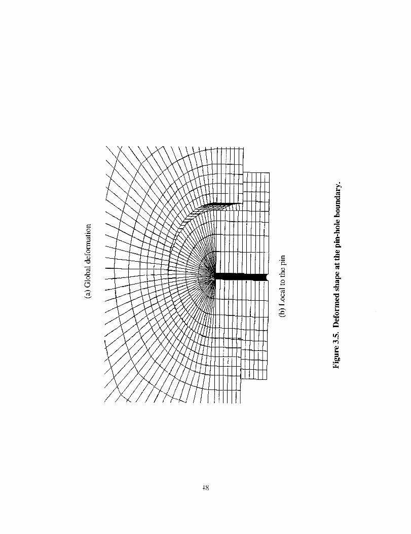
3.5.1.1Deformed Shapes
Figure3.5showtheglobalandlocalto pin deformedshapesof thejoint ata load
levelof 156MPa. As canbeseen,thepin loosescontactwith theplatefrom 0 = 0°to 900
andthenit maintainscontactandtheholeisdeformedintoanelliptic shape.
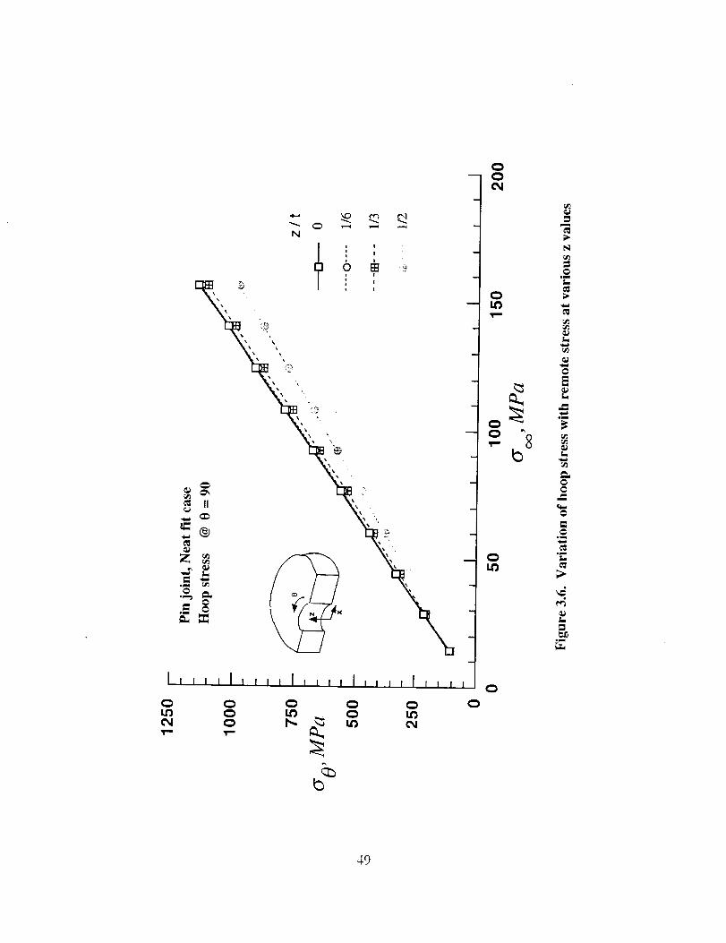
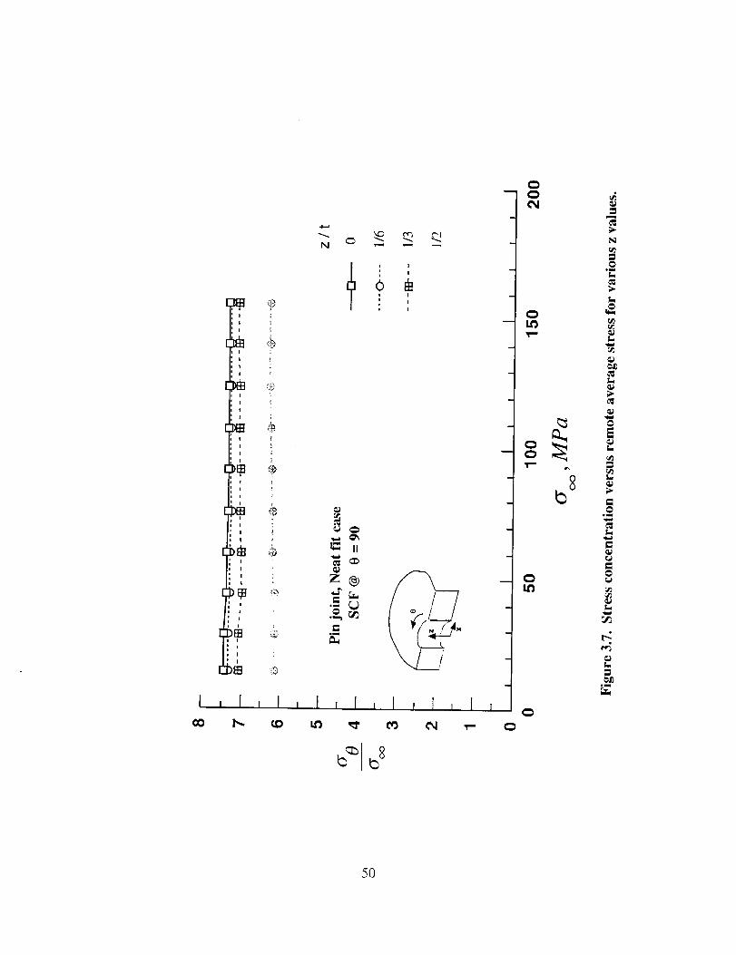
3.5.1.2Contact Non-linearity
Theeffectof contactnon-linearityon localstresseswasexaminedby analyzingthe
hoopstressat0 = 90°on theholeboundaryof theplates.Figure3.6showsthevariationof
% with remoteappliedstress(c_) atvariousvaluesof 'z' at0 = 90°. As canbeseenG0
varieslinearlywith _. Thesameresultsareplottedasstressconcentrationfactor(SCF=
% / _) in Figure 3.7. The SCF is maximum for the bottom plate at Z = 0 (about 7.36) and
lowest at z/t =0.5 (6.2) at the top surface of the plate.
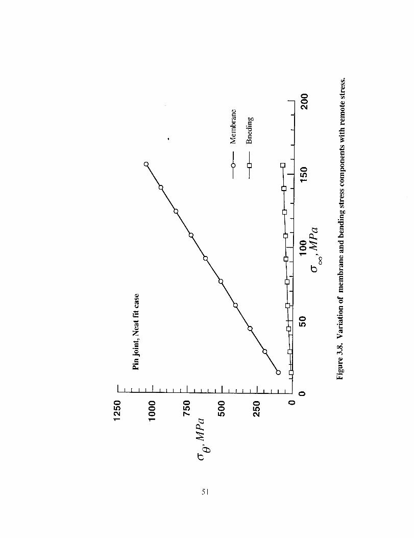
Figure 3.8 shows a linear variation of membrane and bending stresses with or.
Membrane stress is the average stress through the thickness and bending stress is half the
difference between the top and bottom surfaces of the bottom plate at 0 = 90 °. As can be
seen the bending component is negligible compared to the membrane stress. The
38

membraneSCFwas6.78andbendingSCFwas0.57.Therefore,for asmoothfit rivetjoint,
thelocalstressfield varieslinearly with the applied remote stress.
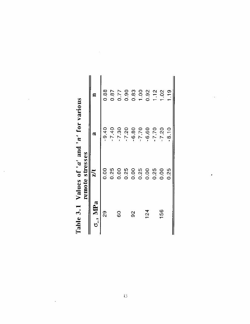
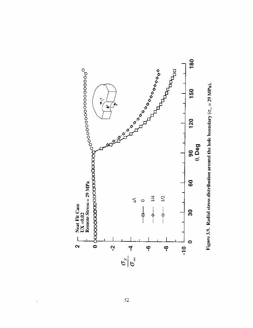
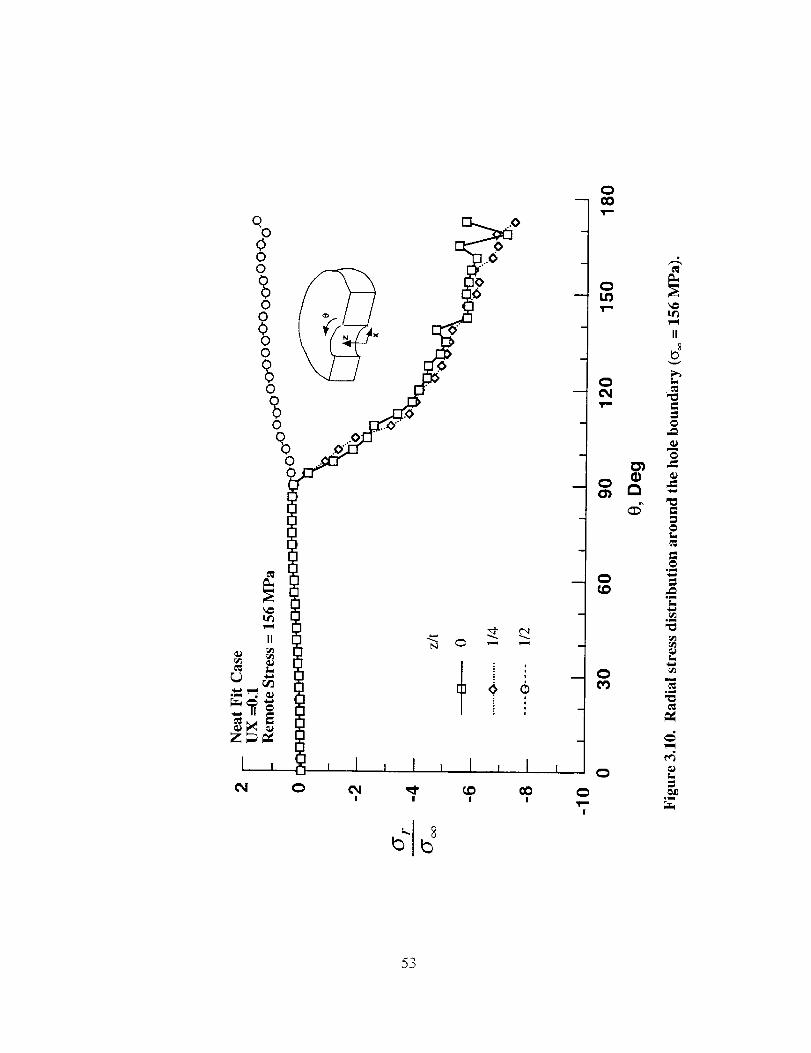
3.5.1.3 Radial Stress Distribution at the Hole Boundary
Figures 3.9 and 3.10 shows the contact (radial) stress distribution on the hole
boundary for remote applied stress of 29 and 156 MPa respectively. Radial stress is
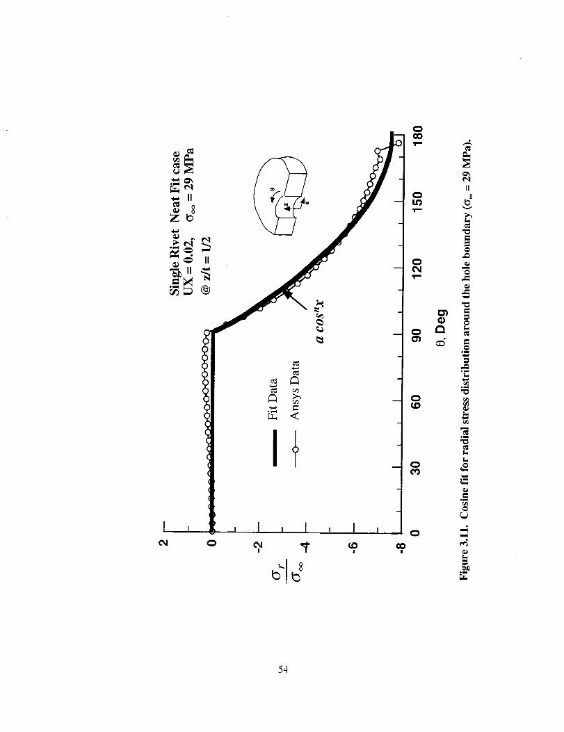
maximum at e = 180 ° for the plate. The radial stress can be approximated by cosine
function as shown in Figure 3.11 (see thick solid curves). These cosine functions can be
represented in the form of
°'r = a cos n 0
o"
Values of 'a' and 'n' for various levels are given by the following table.
Table 3.1 Values of 'a' and 'n' for variousremote stresses
_, MPa z/t a n
29 0.00 -9.40 0.88
0.25 -7.40 0.87
60 0.00 -7.30 0.77
0.25 -7.20 0.90
92 0.00 -6.80 0.83
0.25 -7.70 1.00
124 0.00 -6.60 0.92
0.25 -7.70 1.12
156 0.00 -7.20 1.02
0.25 -8.10 1.19
The rivet contact angle is defined as the angle over which the radial compressive. This angle
was found to be nearly 900 for -3t/8<z<3t/8. Note that contact stress is zero at 0 = 90 ° for
most of the locations through the thickness. Results at z = tp/2 (comer location) may not be
accurate because they are being affected by rivet head contacts.
.39
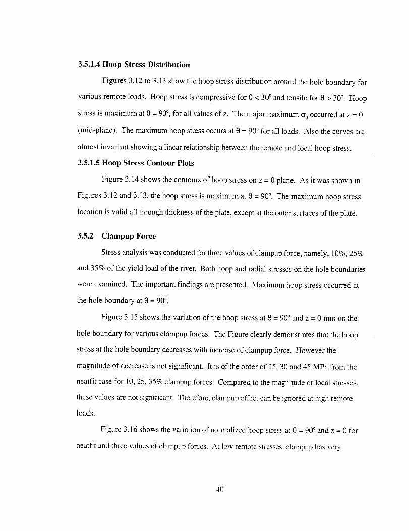
3.5.1.4Hoop Stress Distribution
Figures 3.12 to 3.13 show the hoop stress distribution around the hole boundary for
various remote loads. Hoop stress is compressive for 0 < 300 and tensile for 0 > 30 °. Hoop
stress is maximum at 0 = 90 °, for all values of z. The major maximum _0 occurred at z = 0
(mid-plane). The maximum hoop stress occurs at 0 = 90 ° for all loads. Also the curves are
almost invariant showing a linear relationship between the remote and local hoop stress.
3.5.1.5 Hoop Stress Contour Plots
Figure 3.14 shows the contours of hoop stress on z = 0 plane. As it was shown in
Figures 3.12 and 3.13, the hoop stress is maximum at 0 = 90 °. The maximum hoop stress
location is valid all through thickness of the plate, except at the outer surfaces of the plate.
3.5.2 Clampup Force
Stress analysis was conducted for three values of clampup force, namely, 10%, 25%
and 35% of the yield load of the rivet. Both hoop and radial stresses on the hole boundaries
were examined. The important findings are presented. Maximum hoop stress occurred at
the hole boundary at 0 = 90 °.
Figure 3.15 shows the variation of the hoop stress at 0 = 90 ° and z = 0 mm on the
hole boundary for various clampup forces. The Figure clearly demonstrates that the hoop
stress at the hole boundary decreases with increase of clampup force. However the
magnitude of decrease is not significant. It is of the order of 15, 30 and 45 MPa from the
neatfit case for 10, 25, 35% clampup forces. Compared to the magnitude of local stresses,
these values are not significant. Therefore, clampup effect can be ignored at high remote
loads.
Figure 3.16 shows the variation of normalized hoop stress at 0 = 90 ° and z = 0 for
neatfit and three values of clampup forces. At low remote stresses, clampup has very
4O
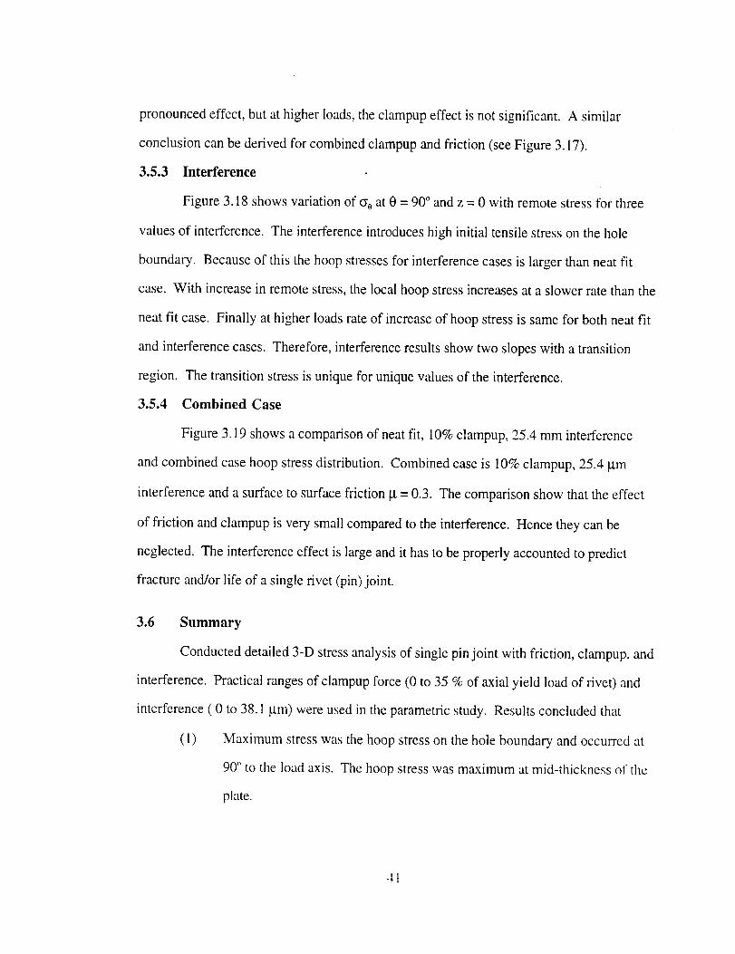
pronouncedeffect,butathigherloads,theclampupeffectisnotsignificant.A similar
conclusioncanbederivedfor combinedclampupandfriction (seeFigure3.17).
3.5.3 Interference
Figure3.18showsvariationof cy0at0 = 90"andz = 0 with remotestressfor three
valuesof interference.Theinterferenceintroduceshighinitial tensilestressonthehole
boundary.Becauseof this thehoopstressesfor interferencecasesis largerthanneatfit
case.With increasein remotestress,thelocalhoopstressincreasesataslowerratethanthe
neatfit case.Finallyathigherloadsrateof increaseof hoopstressis samefor bothneatfit
andinterferencecases.Therefore,interferenceresultsshowtwoslopeswith atransition
region. Thetransitionstressisuniquefor uniquevaluesof theinterference.
3.5.4 Combined Case
Figure3.19showsacomparisonof neatfit, 10%clampup,25.4mm interference
andcombinedcasehoopstressdistribution.Combinedcaseis 10%clampup,25.4p.m
interferenceandasurfaceto surfacefriction la= 0.3. Thecomparisonshowthattheeffect
of friction andclampupisverysmallcomparedto theinterference.Hencetheycanbe
neglected.Theinterferenceeffectis largeandit hastobeproperlyaccountedto predict
fractureand/orlife of asinglerivet (pin)joint.
3.6 Summary
Conducteddetailed3-Dstressanalysisof singlepinjoint with friction,clampup,and
interference.Practicalrangesof clampupforce(0to 35% of axialyield loadof rivet)and
interference( 0to 38.1gin) wereusedin theparametricstudy.Resultsconcludedthat
(1) Maximumstresswasthehoopstressontheholeboundaryandoccurredat
90"to theloadaxis.Thehoopstresswasmaximumatmid-thicknesso1'the
plate.
4t
(2)
(3)
(4)
(5)
(6)
The contact angle was found to be nearly 1800 .
Elastic friction had negligible effect on local stresses (hoop) and hence it can
be ignored.
Clampup effect was dominant at low applied loads. Clampup decreases the
local hoop stresses. But at high applied loads, clampup effect is small.
Interference was a major factor that impacted the local stresses (hoop stress)
around the rivet hole. Interference introduces local tensile hoop stress at the
rivet hole. This initial stress reduces the rate of increase of local stresses
with remote loads. This causes the local hoop stresses to be lower than the
neat fit results at high load levels.
Contact, friction and rivet clampup nonlinearities were confined to low axial
loads. At high loads, the response is nearly linear.
a2
O0 O0 I_- O) O0 00_ _- 0 _r-
0 0 0 0 0 0 0 0 0 0
I I I I l I I I I I
0 od 00_J 00_ 00d 00J
0 0 0 0 0 0 0 0 0 0
Ob 0 OJ "_" _0
+3
m
w
_...._
II .........
N i _'--_:::::::_:
."4%-_'.
e,i
Qm
om
,u
44
_rm
E
--/_=II
i
E
,m
0
t.
I
_m
45
°,m
,m.
.im
=,u
_d
L.
46
C_C_u'_,Tin
C_C_
,Tin
Ec:)m
C.)
C_
oW
r-
omL.
r.-
Em
,m
omm
z_
om
0
c_
©©
c_0
m
em
ell
_g
!
!
I
l
I
II, ,, ,I, ,,, I, ,It I,, ,,I l, ,,
i
=
_mL.
Qm
_9
N C_ ,.. ,-,
!
I
I
i
®
. !
, !
,,._j
I I I w I I I J I i I , t i I i
m
m
m
i
00
L_
0L_
t_.
@
eli=
@.mr
=
@
=
5O
L_ C_ L_ _ U'_
'r- T-" _
00
C_
0L_
0
L.
Z-,
gWl
_rJ
z.,
,m
om
olm_r_
z_
_D_mm
31
m
% ++0
! °.lJ_°_"
t",l
11
i=I
[E J I
!
l I
!
I
]
o ?
, I , I
! !
!
II
lu
0
v_
52
11
r_
! u 1.0
IIg
0
i
0 =
r,_
,m
53
! !¢,D
! !
OL_
O(N
O _
OI,D
O
II8
_m
m
,m
L
_m
54
I
I
0
0
0(D
0
I
I1
t3
m
=
e_
_-|
Lm
,u
55
I
t_
11
|
c_
II8
t_
L.
gm
gpl,I
L,
L.=
56
57
_J
_5
I1
8
¢)
m
_JJ=
,m
L.
C,J=
,J=
_N
m
L
L.
,m

Q 0
a.,
00
m
i
00
0
0
om
7..
11
11
0m
58
I
L
u'l
0
0
Em
0"r,
r_
0E
,m
1,1
lU
59

c_
¢
!
E
Im
m
L.
II
II
L,
om
60
'°o.
°'°_.
II
II
\
E
II
l
.i
L.
II
C
II
L
?.
mm
.m
6;
z
%
b
C_ I_ C_ C_ C_
C_l C_ I_, It) CM
b
oo
c_
.m
!_,
rd_
L)
caL,
O2
4. TWO RIVET SINGLE LAP JOINT
4.1 Introduction
In this section a single lap joint with two rows of rivets was modeled using 3-D
finite elements. This joint is loaded by remote tension and is restrained by using anti-
symmetric boundary conditions as explained in the following sections. The effects of
clampup and interference on the stress distribution in the hole boundary is presented in this
section.
4.2 Joint Configuration
The two-rivet plate joint configuration with all the geometrical parameters are shown
in the Figure 4.1. This geometry represents a test configuration used in reference [31 ]. The
plan and sectional view of a two rivet, single lap joint shown in Figure 4.2 was analyzed.
The rivet shank was straight with 1.6 mm radius R r and 2 mm height. The rivet has two
button heads. The head radius and depth were 2.55 mm and 1 mm respectively. The two
plates, top and bottom were 145 mm long, 20 mm wide (w) and 1 mm thickness (t). The
spacing (s) between the rivet centers was 20 mm. The edge distance was (Ed) 10 mm and
the length L was 125 ram.
The joint was loaded in tension with an uniform displacement Uo. The average
remote stress was O'oo. The two ends of the joint were supported laterally, to simulate the
experimental condition, as shown in Figure 4.2. The Cartesian co-ordinate system selected
in modeling is also shown in Figures 4.1 and 4.2. The X, Y, Z represents the global co-
ordinate system and x, y, z represents the local co-ordinate system used for plotting results.
63
¥ 7
EO
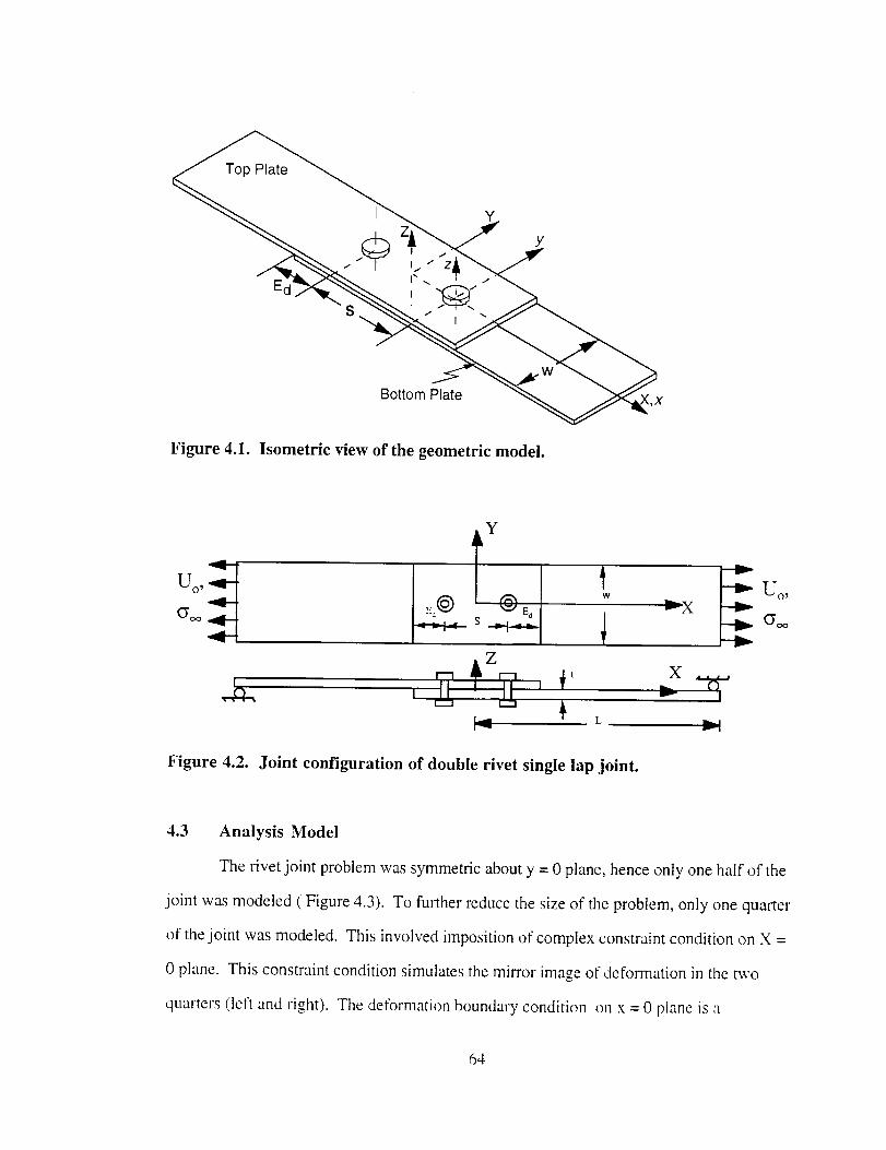
Figure 4.1. Isometric view of the geometric model.
Y
_X
Z
I 1
Joint configuration of double rivet single lap joint.Figure 4.2.
4.3 Analysis Model
The rivet joint problem was symmetric about y = 0 plane, hence only one half of the
joint was modeled ( Figure 4.3). To further reduce the size of the problem, only one quarter
of the joint was modeled. This involved irnposition of complex constraint condition on X =
0 plane. This constraint condition simulates the mirror image of deformation in the two
quarters (left and right). The deformation boundary condition on x = 0 plane is a
64

combination of anti-symmetry and skew symmetry. The boundary conditions can be
expressed by the following constraint equations:
U(0, y, -z) = -U(0, y, z)
v(o, y, -z) = v(o, y, z)
w(o, y, -z) = -w(o, y, z)
These boundary conditions reduce the finite element model to one quarter of the
joint (see Figure 4.4).
AntisymmetricPlane
t
Figure 4.3. Sectional 3-D view showing cyclic anti-symmetry.
65
Z
w/2
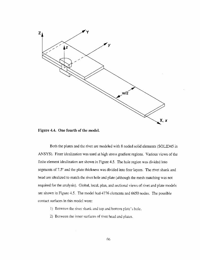
Figure 4.4. One fourth of the model.
Both the plates and the rivet are modeled with 8 noded solid elements (SOLID45 in
ANSYS). Finer idealization was used at high stress gradient regions. Various views of the
finite element idealization are shown in Figure 4.5. The hole region was divided into
segments of 7.5 ° and the plate thickness was divided into four layers. The rivet shank and
head are idealized to match the rivet hole and plate (although the mesh matching was not
required for the analysis). Global, local, plan, and sectional views of rivet and plate models
are shown in Figure 4.5. The model had 4776 elements and 6650 nodes. The possible
contact surfaces in this model were:
1) Between the rivet shank and top and bottom plate's hole.
2) Between the inner surfaces of rivet head and plates.
66

3) Between the bottom surface of top plate and top surface of bottom plate.
These contact surfaces were modeled using 5-noded 3-D surface to surface contact
elements represented by CONTAC49 in ANSYS code. Each target node has the possibility
of contacting four elements. The model contained 2588 contact elements.
i i i I 1 I
Plan view
Bolt
Joint assembly
Top & bottom platesand contact surface
Figure 4.5. Various views of the rivet joint finite element model.
The loading imposed on the model was a uniform displacement 'Uo' at X = L. In
summary, the following boundary conditions are applied on the model:
(1) Symmetry on y=0 plane.
(2) Constraint equations on nodes at x=0 plane.
(3) Uy = 0 at x = L, y = 0 and z = 0 (for restricting rigid body motion).
(4) The loading (displacement) u = uo was imposed at x = L (125 mm_ plane.
67
Aluminumalloy2024-T3Alcladpropertieswereusedin theanalysis.Therivetsare
2024(typeDD) aluminum.TheelasticmodulusE = 68,950MPa,Poisson'sratio v =
0.3, yield strength of 270 MPa and ultimate strength of 270 MPa.
4.4 Analysis Cases
Two types of non-linearities were expected in the model, viz., nonlinear contact
boundary and large rotation. Therefore, large deformation and non-linear contact strategy
were used in the analysis. A commercial code ANSYS 5.3 was used. The nonlinearities
were modeled by modified Newton-Raphson iteration algorithm. The Lagrange multiplier
and penalty method were used for contact modeling. The defined gap/penetrations and
contact stiffnesses are about 0.01Hs and 2000 N/ram 2 (about 3% of the elastic modulus of
the plate material, which was within the recommended range) respectively. But for
interference cases gap/penetration value used was 0.025Hs. Where Hs was the smallest
element size in the model, which was 0.25 man. The residual force convergence criteria was
used at every node to establish the convergence of the non-linear solution. Relative error in
the nodal residual forces was less than 0. 1% to 1% of total applied force as a convergence
criteria.
The analysis was conducted for three different complexities that occur in the joint.
They are friction between contacting surfaces, rivet clamp-up, and rivet interference.
Analytical modeling of each of these parameters is explained in section 2 and is summarized
in the following sections. The analysis was conducted by incrementally loading the joint to
an applied remote load of about 130 MPa or about U o = 0.3 ram.
68
4.4.1 Friction
Friction between the contact surface was modeled as elastic coulomb friction. The
surface tangent stiffness KT was selected to be KN/100, where KN was the normal contact
stiffness. The tangential friction force at the contacted nodes was the product of friction
coefficients and the normal force. The sliding friction coefficients used in the analysis were
0, 0.3 and 0.8. The friction coefficient value of zero represents the smooth contact.
4.4.2 Rivet Clamp-up
As explained in section 2.3 the rivet clamp-up was introduced by changing the
length of the rivet shank. By shortening the rivet length compared to the thickness of the
two plates clamp-up force was introduced. A separate stress analysis was conducted to
establish a relation between clamp-up force and rivet shortening. This relationship was
found to be linear (refer to Figure 3.4). The clampup equation was given by
Clampup force, F c = 64,054 * AL
where AL is the rivet shortening (Trs - Tp) in mm
The amount of rivet shortening for clamp-up force of 10%, 25%, 35% rivet yield
force was calculated. These values were 7.64, 19.1 and 26.7 p.m respectively. The analysis
was conducted for all these values of rivet shortening.
4.4.3 Rivet Interference
Rivet interference was introduced by increasing the radius of the rivet (P_) in relation
to the hole radius (Rh). Three values of interference 2(Rr-Rh) chosen were 12.7,
25.4 and 38.1 _tm. These values bound the real values experienced in the aircraft industry.
4.5 Results
Results of the analysis conducted for various cases are represented in this section.
First, neat fit (zero surface-surface friction) results are presented. Then the effects of
69
fi'iction,clamp-upandinterferenceon localstresseswereexamined.Theprimaryfocuswas
on themaximumhoopstresson theholeboundaryandthehoopstressat 90° to thex-axis.
Thesecondcaseis wherethehoopstressismaximumfor openholeproblems.
4.5.1 NeatFit Results
4.5.1.1 Deformed Shapes
Figure 4.7 shows the sectional view of the deformed shape of the model. Notice
that the two plates slided one past the other at the left end of the model. This is the true
deformation expected if the complete half model was analyzed. This deformation pattern
confirms the approximation of the boundary conditions imposed on X = 0 plane. The
close-up view of the model at the rivet is shown in Figure 4.8. Notice that the rivet is in
contact with top plate on the right side and bottom plate left side. The right side of bottom
plate and the left side of top plate are separated from the rivet shank. The two plates are
separated from each other on the loaded side. In the 3-D model like this problem, all
separation and contact are only partial and they change along the polar (9) direction of the
rivet. Figure 4.9 shows the superposed view of the two quarters of the model. This depicts
the local joint rotation and deformation.
4.5.1.2 Contact Nonlinearity
The effect of contact nonlinearity on local stresses was examined by analyzing the
hoop stress at e = 90 ° on the hole boundary of the plates. Figure 4. I0 shows the variation
of eye with remote applied stress ((y) at various values of 'z' at 0 = 90 °. Except at low
values of applied stress, cy < 30 MPa, go varies linearly with 6. The same results are
plotted as stress concentration factor (SCF = (y_ / (_) in Figure 4.11. Again, the SCF is
maximum for the bottom plate at Z = 0, which is about 5.7,
Figure 4.12 shows almost linear variation of membrane and bending stresses with
Q. Membrane stress is the average stress through the thickness and bending stre,_s is half
7O

thedifferencebetweenthetopandbottomsurfacesof thebottomplateat 0= 90°. Both
membraneandbendingstressesvary linearlythroughthethickness.ThemembraneSCFs
were4.75and3.4for thebottomandtopplateswhereasthebendingSCFwere 1.2and0.6
for thebottomandtopplatesrespectively.
4.5.1.3Radial StressDistribution at the Hole Boundary
Figures4.13and4.14showsthecontact(radial)stressdistributiononthehole
boundaryfor remoteappliedstressof 45and84MParespectively.Radialstressis
maximumat0 = 180°for thebottomplateand0 = 0° for thetopplate(notshown).The
radialstresscanbeapproximatedbycosinefunction(seethick solidcurves).Thesecosine
functionsareof theform shownbelow:
o',. =acos n 0
o=
Note that contact stress is zero at 0 = 90 ° for most of the locations through the thickness.
Results at z = -1.0 (corner location) may not be accurate because they are being affected by
rivet head contacts.
4.5.1.4 Hoop Stress Distribution at the Hole Boundary
Figures 4.15 and 4.16 shows hoop stress distribution on the hole boundary for the
applied stress of 45 and 84 MPa respectively. The hoop stress peaks at 0 = 90 ° for values
of z through the thickness. The maximum stress is at z = 0.0, which is about 5.7 times that
of the remote stress.
4.5.1.5 Hoop Stress Contour Plots
Figure 4.17 shows the hoop stress contour plots on both top and bottom plates.
The plate is sectioned at x = 0 plane to examine the location of maximum sq through the
width. Results on Figure 4.17 concludes that for a smooth fit case. the location of the
maximum hoop stress is on the hole boundary and at z = 0.0.
71
In all theresultspresentedsofar, hoopstresson theholeboundaryis highestandit
occursin thebottomplateat theinterfacebetweenthetwoplates.
4.5.2 Elastic Friction
Stressanalysiswasconductedfor elasticfrictionvaluesof 0.3and0.8for applied
remotestressvaryingfrom 0 to about140MPa. Bothradialandhoopstressdistribution
alongtheholesurfaceandthroughthethicknesswereexaminedfor all casesandcompared
with neatfitresults.Comparisonof resultsshowedvery littleeffectof friction onmagnitude
andlocationof peakvalues.Tensilestressesin thebottomplatewerehigherthanthatin the
topplate.Therefore,only resultsfor thebottomplatearepresentedfor thiscaseandall
otherremainingcases.Figure 4.18 and 4.19 shows hoop stress variation along the hole
surface at various plate thickness locations for 1.1= 0.3 and bt = 0.8 respectively. For both
cases c e is maximum at 0 = 90 ° and z = 0.
Figure 4.20 shows variation of % at 0 = 90 ° with remote stress ( cy ) for I.t = 0, 0.3
and 0.8. Results of p =0 and p = 0.3 were almost identical and at low values of ¢y,, bt =
0.8 stresses were smaller than bt = 0 case, but for _® > 55 MPa, all three curves merged.
Therefore, elastic friction alone has very little effect or no effect on joint stresses.
4.5.3 Clampup Force
Stress analysis was conducted for three values of clampup force, namely, 10%, 25%
and 35% of the yield load of the rivet. Both hoop and radial stresses on the hole boundaries
were examined. The important findings are presented. Maximum hoop stress occurred at
the hole boundaI3, except for very.' small value of remote applied stress. At ve_, low applied
stress, the maximum hoop stress occurred in the interior of the plate, this may be because of
pinching effect caused by clamping.
72
Figures4.21to 4.23showsthe_3_stressdistributionontheholeboundaryfor 10%
clampupforceat remotestressesof 45.7,94.5and 143.7MParespectively.Maximum
hoopstresslocationchangedfrom 75° atlow loadlevelsto 90° athigh loads. Againthetwo
plate'sinterfacelocationwashighlystressedregionin theplates.Table4.1summarizesthe
magnitudeandlocationof maximumhoopstressfor all threeclampupforcesandvarious
appliedstressvalues.Thelocationof maximumstressis at75° for both25%and35%
clampupforcefor highervaluesof appliedstress.
Thetablealsoliststhehoopstressvaluesat z = 0 and0 = 90°,andthedifference
comparedtothemaximumstress.Thedifferenceincreaseswith increasedclampupforce
butdecreaseswith increaseof appliedstress.For 10%clampupforce,onecanneglectthe
differencefor cy > 50MPa.Knowing% at0 = 90° andz = 0, for anycondition,onecan
calculatebackthemaximumvalueof thehoopstressandits locationusingthetable4.I
results.
Figure4.24showsvariationof _eat 0= 90oandz = 0 for thethreevaluesof
clampupforcesandfor various_=loads.TheFigureclearlydemonstratesthat,asexpected
thehoopstressat theholeboundaryalsodecreaseswith increaseof clampupforce, The
relationshipbetweentheclampupforceandthehoopstresscanbeexpressedby asimple
equation:
(O'0)Cl_mp,,p= (O'0)N_,_, -- 31Co
where C,_ is the clampup stress, defined as clampup force divided by clamping area of the
plate. In the equation, all stresses are expressed in N/ram 2 (MPa). At low applied stresses,
clampup has nonlinear effect on the local stresses.
Figures 4.25 and 4.26 show the effects of clampup on membrane and bending
components of the stress on the hole boundary at 0 = 90 °. Membrane stresses decreases
with increase in clampup, where as the bending stresses increases.
73
Figure 4.27 shows the variation of cyJcy® with radial distance from the hole
boundary. The clampup effect is confined to clamped region, beyond that the hoop stress
are unaffected by the clampup; particularly for higher remote stress (o" = 140 MPa).
However at lower load levels, say 65 MPa, the influence of clampup goes slightly beyond
the clampup region. The magnitude of change is minimal. Hence it terms of crack initiation
and crack growth, clampup can increase the crack initiation life but once the crack has
grown beyond the rivet head, clampup has no effect on crack growth.
4.5.4 Clampup and Elastic Friction
This analysis was conducted with the intention that the clampup force would increase the
normal force between the plate surfaces and hence the friction effect (the tangential friction
force is equal to the product of the normal force and the coefficient friction). Figure 4.28
shows that friction still does not have any effect on the hoop stress distribution on the hole
boundary. Hence we can conclude that friction has no effect on stress distribution in the
joint.
4.5.5 Interference
Figure 4.29 and 4.30 show the hoop stress distribution around the hole boundary for an
interference value of 12.7 mm and remote stress value of 48.7 and 78.7 MPa respectively.
As can be seen from Figure 4.29 the maximum hoop stress occurs at 0 = 67.5 ° and as the
remote load increases the location of maximum hoop stress shifts to 0 = 75 ° at remote load
of 78.7 MPa (Figure 4.30). This trend can be also be inferred from table 4.2 which lists
location of maximum hoop stress for all interference values. The maximum hoop stress
location varies from 1350 (for low load levels) to about 75" for high load levels.
Figure 4.31 and 4.32 show the radial stress distribution around the hole boundary.
As can be observed the radial stress became negative before 90 ° toE all values of z. This is
because of the interference effect. Since the rivet shank diameter is greater than that of the
74
plate hole, the rivet is in contact with more than quarter of the hole boundary and this
induces compressive radial stresses on the plate hole even for 0 < 90 °.
The effect of interference on hoop stress at z = 0 and 0 = 90 ° is shown in Figure
4.33 and the results are compared with neatfit case. Notice there are three distinct regions
behaving differently. At low applied stresses, the local hoop stresses (co) increases with
increase in interference value and it is larger than the neat fit case. At very large applied
stress, local Go for the neat fit case is larger than all the interference cases. In between these
two regions, the results cross each other. However, interference introduces initial tensile
stress on the hole boundary and the rate of increase of (yodecreases with the amount
interference. The slope of % curve decreases from neatfit to 12.7, 25.4, and 38.1 [am. All
four curves cross each other at different applied stress values. The trend of the curves
indicate that eventually ( at large _=. ) they will all be parallel to each other with neatfit case
having highest cyoand the largest interference having the lowest %. From these results we
can conclude:
1. Because interference case introduces initial tensile stresses at G= = 0, the
alternating component of the local stress due to alternating _,, is lower than the neat fit
results.
2. Slope of the % vs _= is smaller with increased interference. This in effect
reduces the alternating component of the local stress _.
4.6 Summary
Conducted detailed 3-D stress analysis of single lap joint with two rows of rivet
including the effect of friction, ctampup, and interference. Practical ranges of clampup force
(0 to 35 % of axial yield load of rivet) and interference ( 0 to 38. I btm) were used in the
parametric studv. Results concluded that:
75
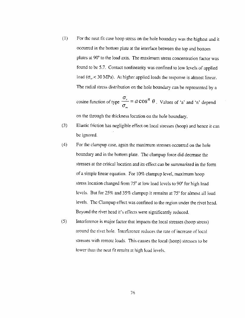
(l)
(3)
(4)
(5)
For the neat fit case hoop stress on the hole boundary was the highest and it
occurred in the bottom plate at the interface between the top and bottom
plates at 90 ° to the load axis. The maximum stress concentration factor was
found to be 5.7. Contact nonlinearity was confined to low levels of applied
load (cy.< 30 MPa). At higher applied loads the response is almost linear.
The radial stress distribution on the hole boundary can be represented by a
o-rcosine function of type -- = a cos" 0. Values of 'a' and 'n' depend
o-
on the through the thickness location on the hole boundary.
Elastic friction has negligible effect on local stresses (hoop) and hence it can
be ignored.
For the clampup case, again the maximum stresses occurred on the hole
boundary and in the bottom plate. The clampup force did decrease the
stresses at the critical location and its effect can be summarized in the form
of a simple linear equation. For 10% clampup level, maximum hoop
stress location changed from 75 ° at low load levels to 90 ° for high load
levels. But for 25% and 35% clampup it remains at 75 ° for almost all load
levels. The Clampup effect was confined to the region under the rivet head.
Beyond the rivet head it's effects were significantly reduced.
Interference is major factor that impacts the local stresses (hoop stress)
around the rivet hole. Interference reduces the rate of increase of local
stresses with remote loads. This causes the local (hoop) stresses to be
lower than the neat fit results at high load levels.
76
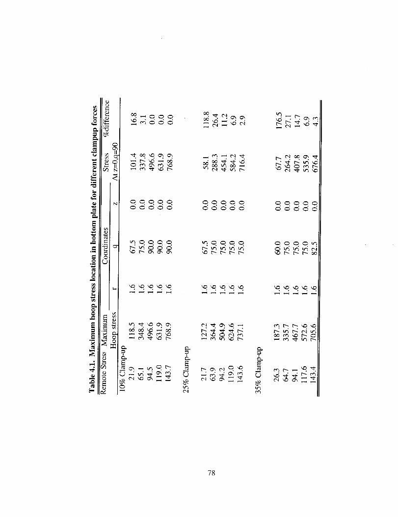
I,
.m
m
o_
0l
E
e
0
r_
e-
©0
_0000..°°,
• ° ° . °
• ° . ° °
0 __0
• . ° .
..,,°00000
E
o!
00000
0000_
78
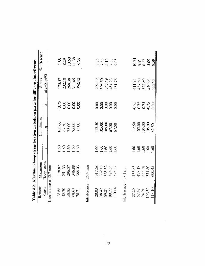
_d
olml
I=.
Im
m
oN
om
¢d
m
1.=
E
om
m:
¢..)
<D
°_
N
OOL_
O
II
ug ,--_ r_ _- ---J-
,--_ ('q (_1 ¢g ¢,g
EE
b_O1
II
..qq_
_1_ _
II
ddo_IIII
• • ° ° °
ug _,, ur-_ I..,..
.
79
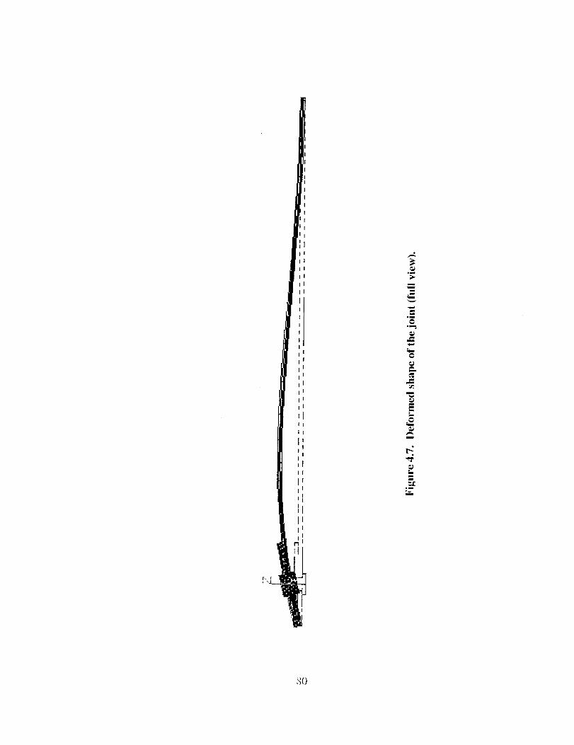
mw
ju
I!
mw
c
_Almu
_Cr_u
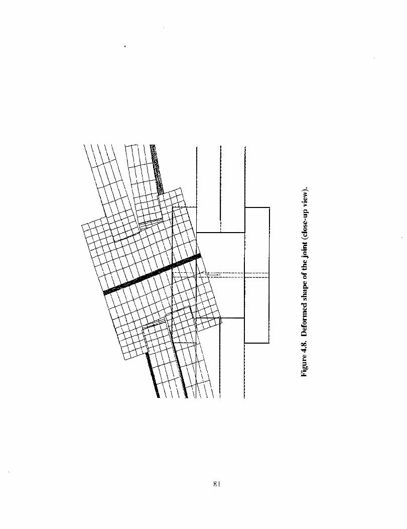
\
\
\\
u
c_om
c/jC_
gm
t_.
Im
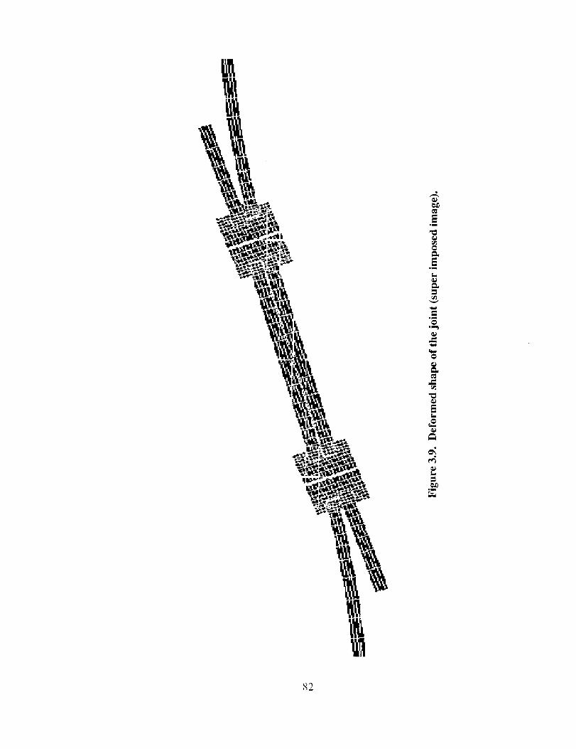
tm_
II
III
z--
0o.I_
_t
E
L.
oil
_2
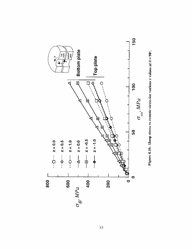
II il il il II II \\ V'
N N N N N N _'E_
I , I , i , I ,O Q Q 0
y,,-
II
=
=
,4
-Ii
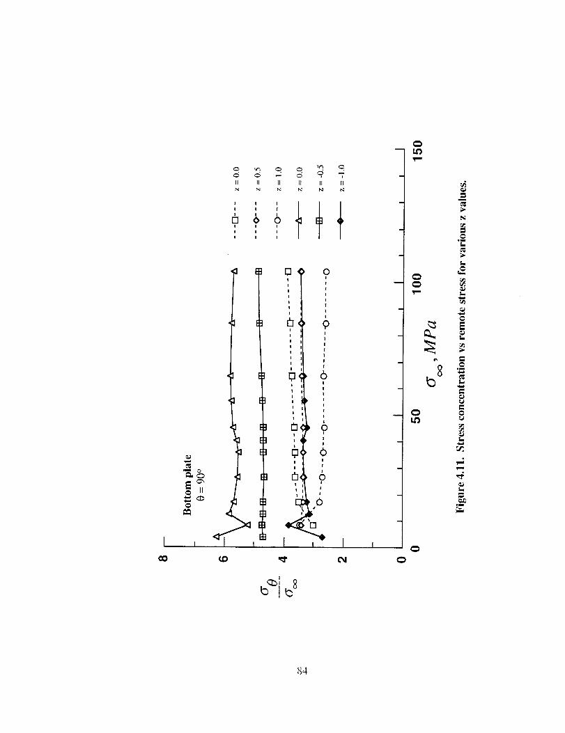
I00
o ,Q.
11 II
N
I I
I I
! I
! !
I I
0 !-_g:,E _
i I
CO
0 0
•-_ o o, -II [I I{ II
!
6I
I
I
D< o!
I
I
I
I
!
!
I!
J
I
!
I
I
t
I
1
I
I
! II!
!
|
i , I
m _,j
0
m 0
8b
N
@.m
6
@
L.
@.J
,4
I.-
.m
_4
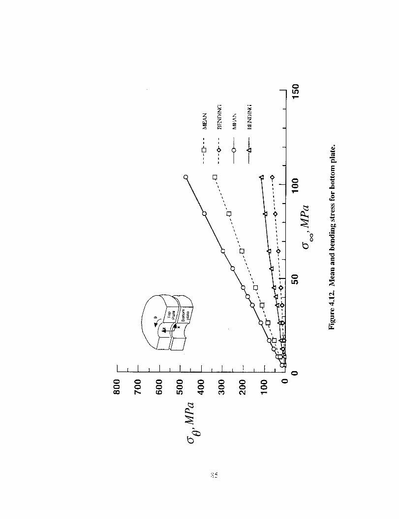
I I
I I
I I
I I
m...,
t_
<_
l,.m.
E
r_
I,=,
+i
,,0
"0
t'-i
,4
I=,
P_
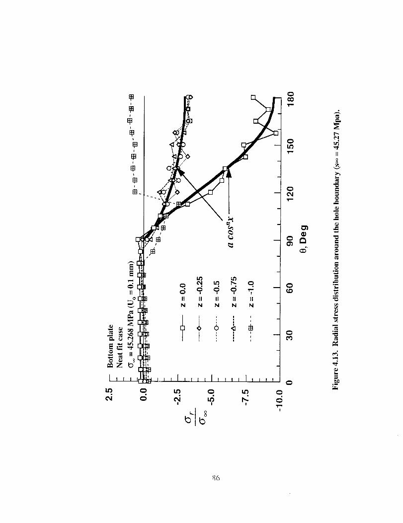
I I I
14'3
0
t.O
I
i
L_I
8
!
I
t"-
II
8
m
=.
@
.m
m
.m
L
J
L
.u
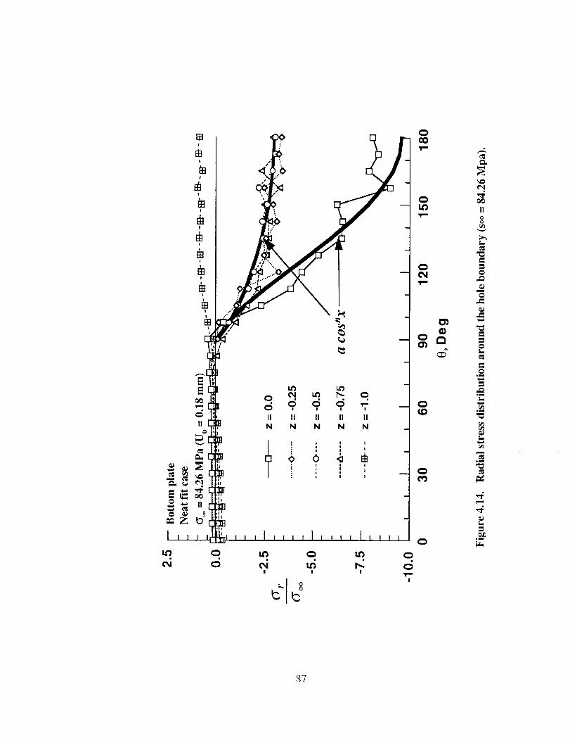
r
_ =
_1" II II II II
I ILl'_ N N N N N
-_ _._:_
,; =_
I I I
C] 8
87
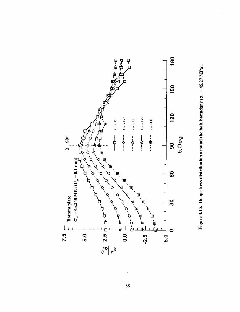
88
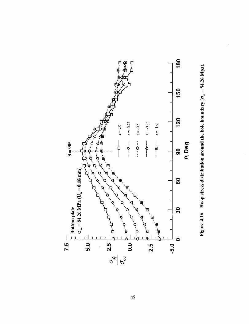
II II II II II
I |
0
0
¢0
t"q
II
m
nw
0i
I
m
!_
_u
m
L
_C
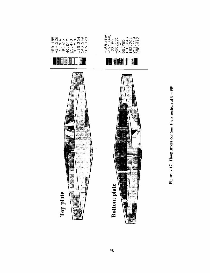
d_... _d_• I l I __ I I I I__
Ili|J [ l
II
I_,
c_
i_.
c_
r_
Im
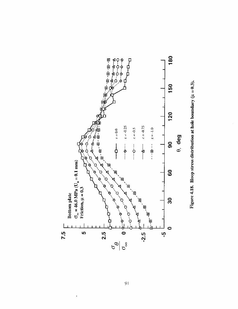
I
,_,_,o..:i Is' ,,"
F..77_",_,_ S o o 9 -:
g46_* ,:..,,.: , _ _ :. _ ; ,
_._'_ _ _. _ _ _,
,,, ,I, ,,, I,_1 ,_
I
I I
I
gT=,,
iT==
0 II
¢D
0¢0
11
l_
m
0
.m
I..
9!

u")
0_1 ¢N
u')|
cO
¢N
¢D
II
2_
,q
92
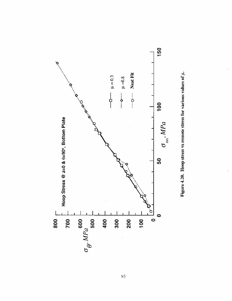
\.m
II ii
\
0 _ _ 0 0 0 0 0_ _ 0 0 0 0 0
0
0
0
0
0
=J
@.m
@E
i=,
=.m
93
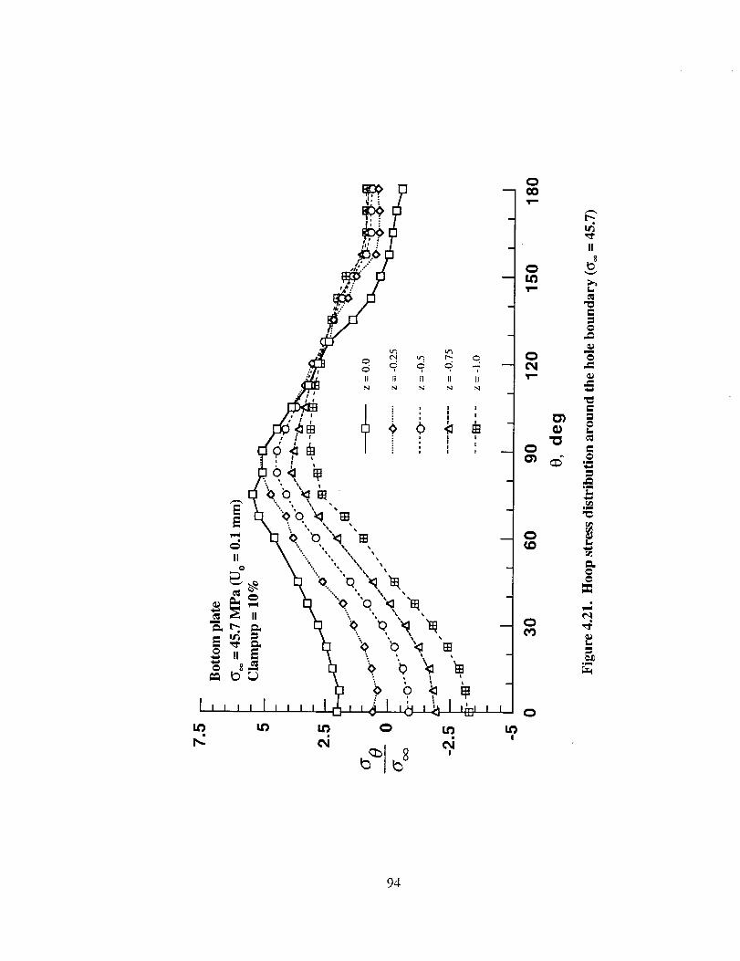
I I I I I I I I I
9'4
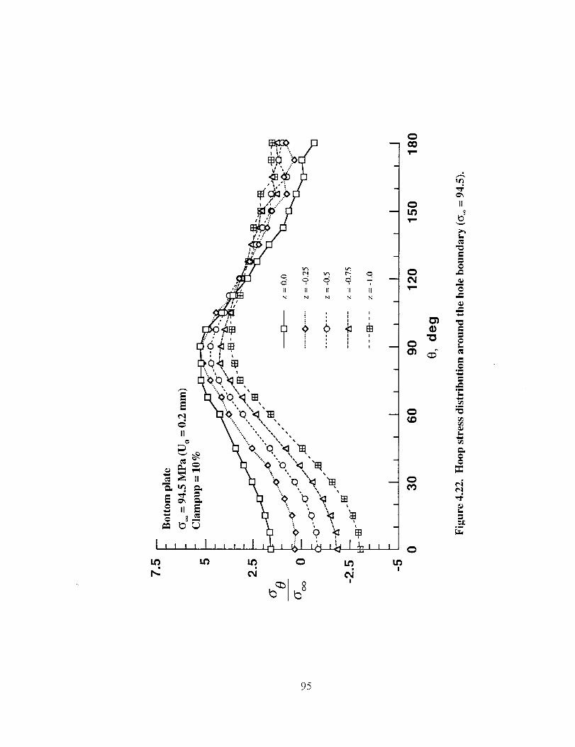
1
t iI I
0 II
L.
0
m
,m
,w
,m
I...
,m
95
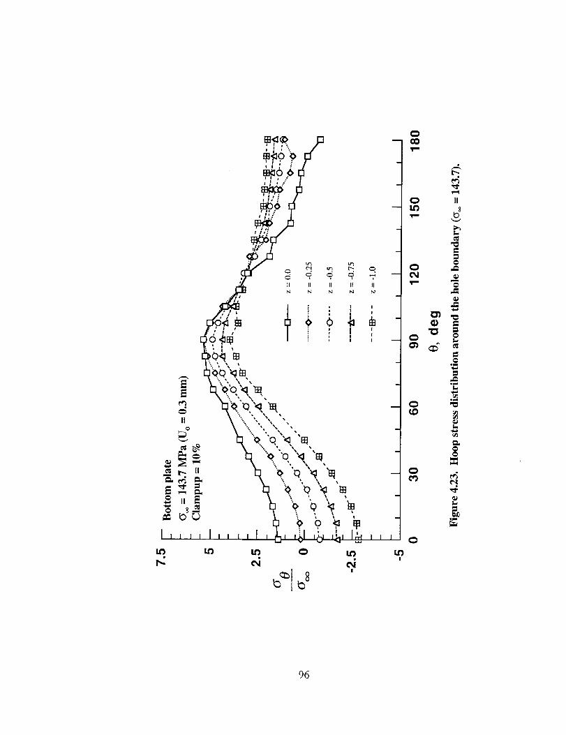
!
!
I
1
I
95
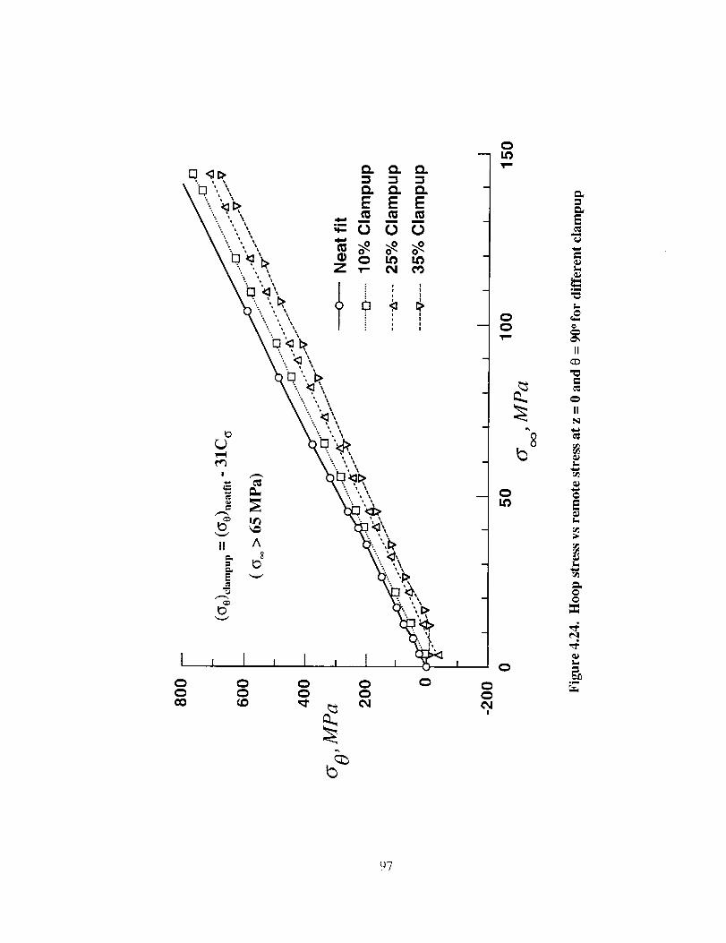
=
t--
_m
il
L
t_
_7
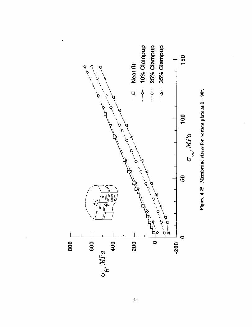
GO
I , I , I
OO_D
!
O
&
II
£
,m
98
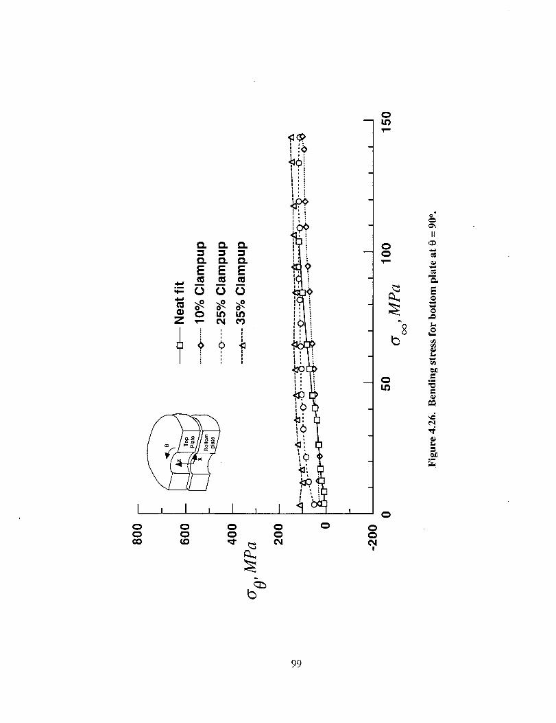
I
O. O. O.
O. O. O.
E E E
_= U U U
Z _- _ 00
i,: 1
1 , I , I ,
O O OO O O00 _D
b
! i :
i
<>
OOC_
O
I
C_LO
O
OLO
O
c
II<D
m_L
L.
,ml
_a
_aL
,m
99
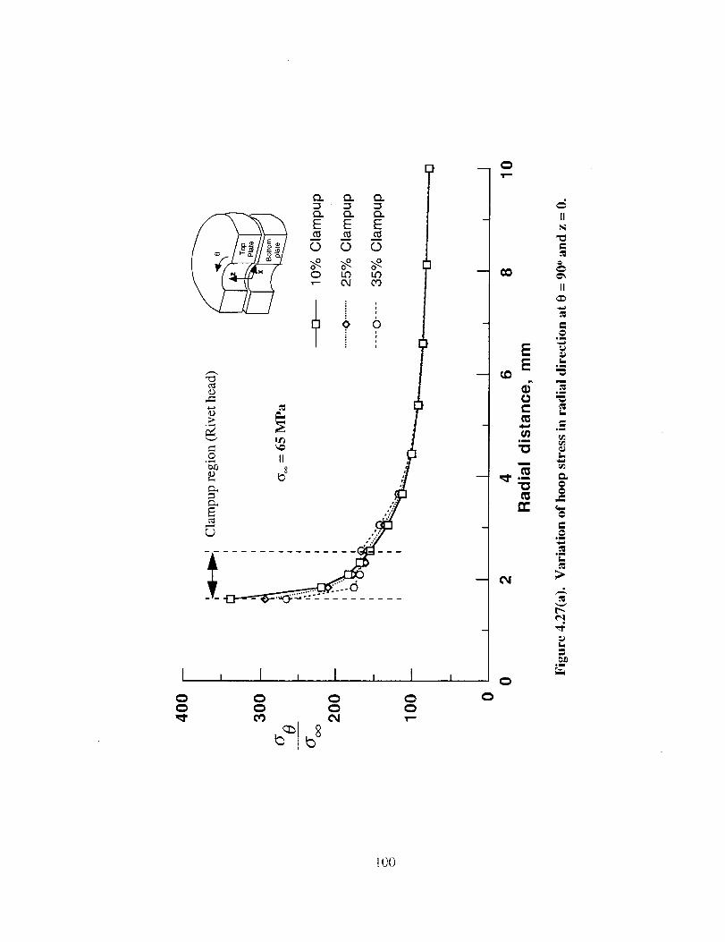
I
I
I , ! .....i I ,
_ 0
EE
e-
|E
m
-- _I'._
rr
II
II
L°_
m
ou
L
l_
.=
o=
p.
r_eq
,mrT
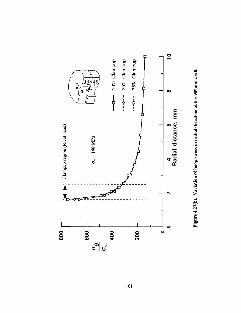
I
I i 1
E E E
0 0 (5
O u3 t_
i :!
|w
O OO
OO
OOIN
i O
m CO
EE
O¢-
im
"Om
mm
IIN
I1
Jm
L,m
m
om
im
0m
,m
,4
lol
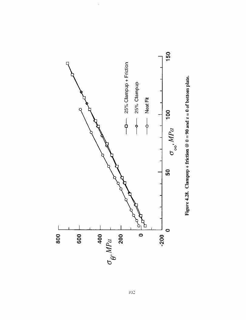
0 0 0
cO +.0
0
1o
ii
m
E
IIN
1=
II
®
om
o_
&+
=
e-t,4
.m
I02
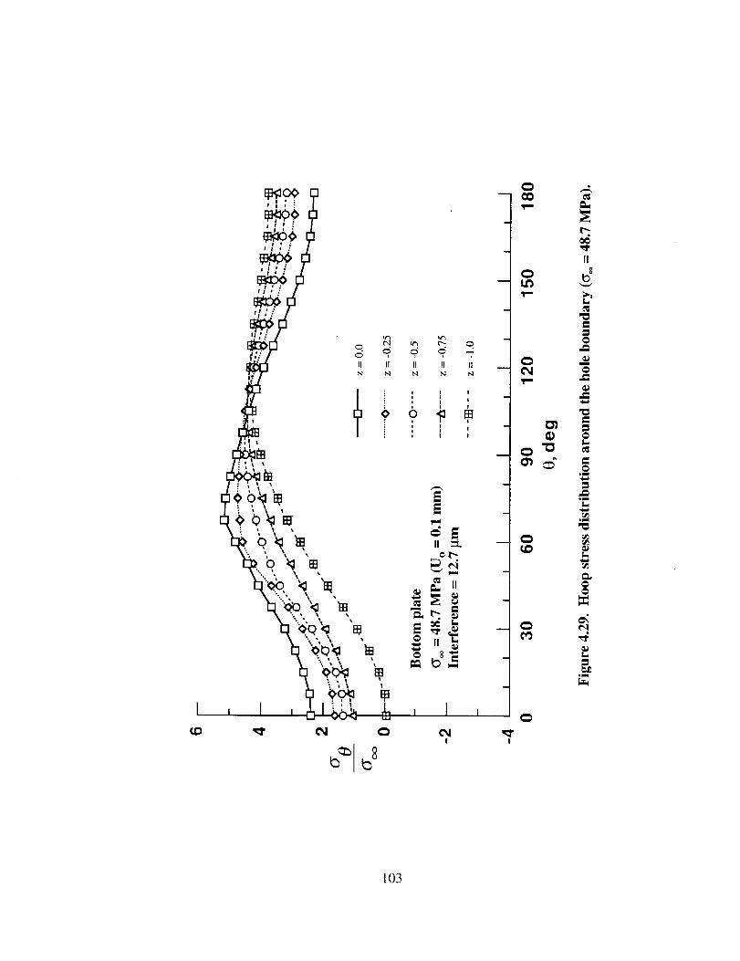
!
103
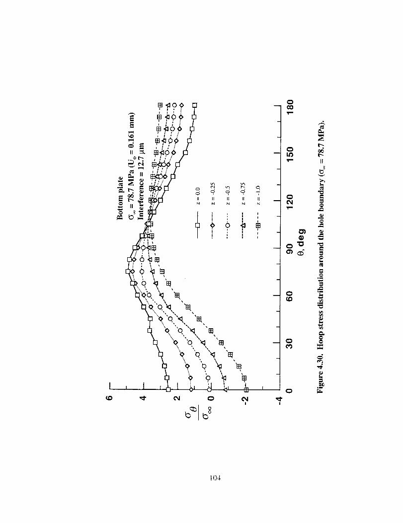
I
I04
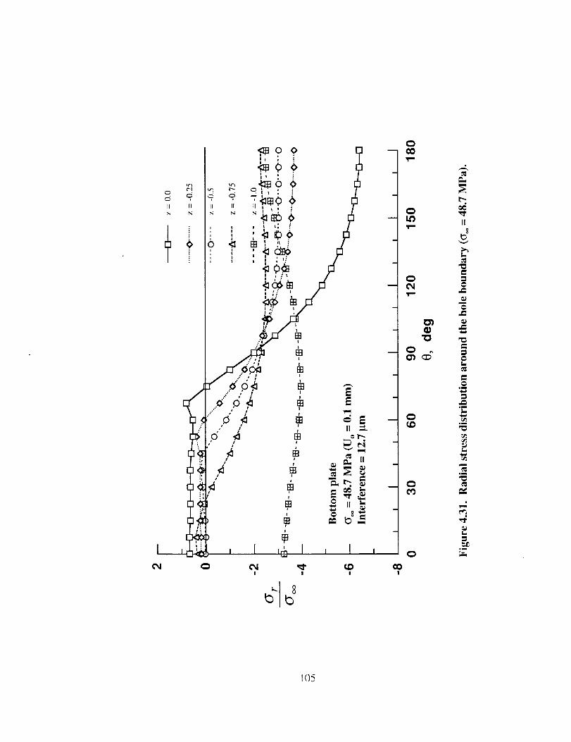
II II
I
!
_0
(,0
II
u
=_
oi
Im
L
m
o_
im
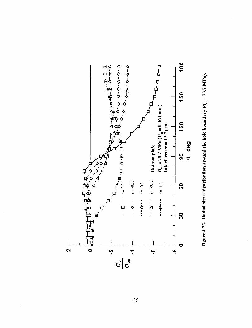
II II II II 11
i I
, 1 i _
I
!
I I
! !
II
_ j
oli
m
gm
m.
o_
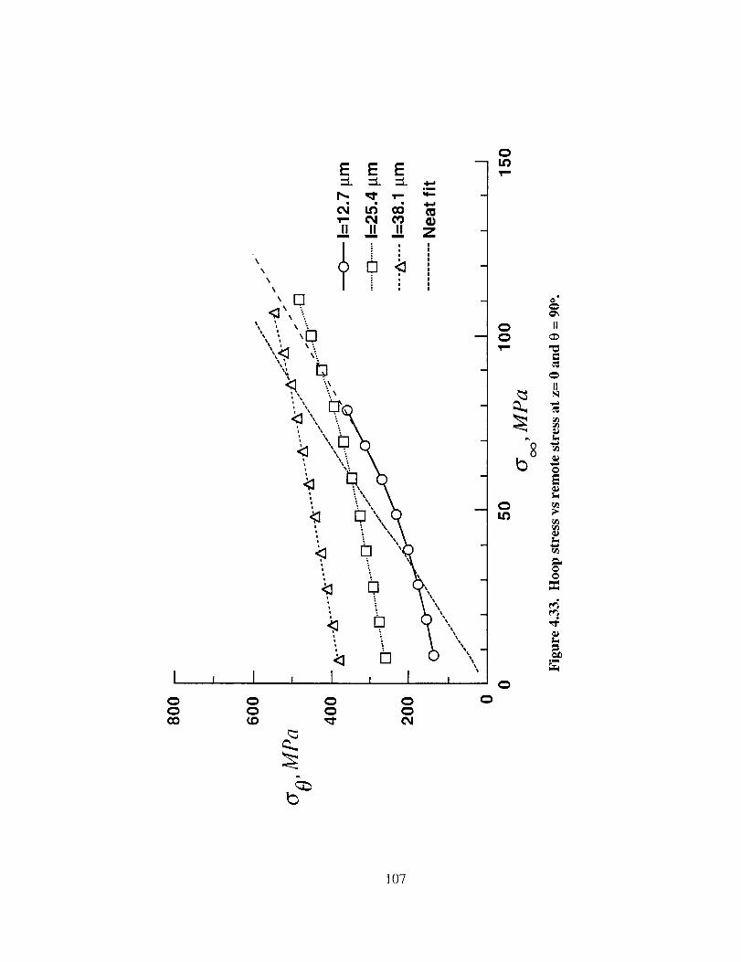
I I
E E E
• I i ; I
\ (_ ' I, _ ,< :
I , I , I ,
CD _ 0_ 0 0
II
I07
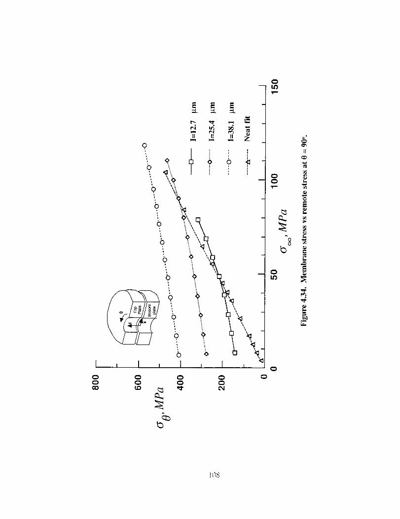
E E E
II II II
0
II
C
E
m.
,m
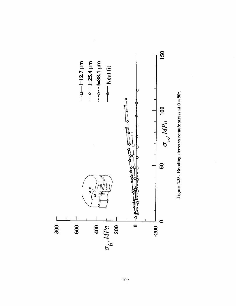
0
cO
I f I00
0 0
(NI
0
00
0
0 j
I!
rll
L..
L,,
,m
u_m.
,m
109
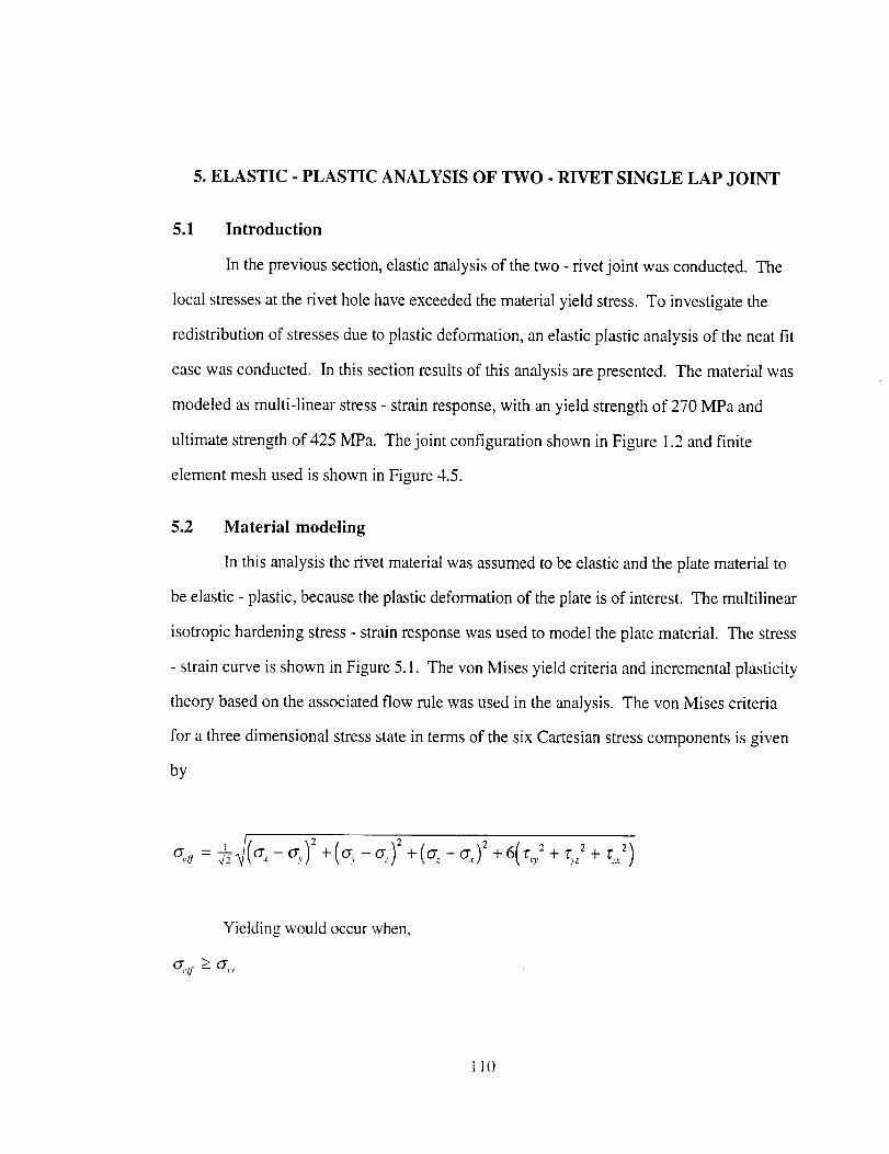
5. ELASTIC - PLASTIC ANALYSIS OF TWO - RIVET SINGLE LAP JOINT
5.1 Introduction
In the previous section, elastic analysis of the two - rivet joint was conducted. The
local stresses at the rivet hole have exceeded the material yield stress. To investigate the
redistribution of stresses due to plastic deformation, an elastic plastic analysis of the neat fit
case was conducted. In this section results of this analysis are presented. The material was
modeled as multi-linear stress - strain response, with an yield strength of 270 MPa and
ultimate strength of 425 MPa. The joint configuration shown in Figure 1.2 and finite
element mesh used is shown in Figure 4.5.
5.2 Material modeling
In this analysis the rivet material was assumed to be elastic and the plate material to
be elastic - plastic, because the plastic deformation of the plate is of interest. The multilinear
isotropic hardening stress - strain response was used to model the plate material. The stress
- strain curve is shown in Figure 5.1. The yon Mises yield criteria and incremental plasticity
theory based on the associated flow rule was used in the analysis. The von Mises criteria
for a three dimensional stress state in terms of the six Cartesian stress components is given
by
Yielding would occur when,
G_,Ij->- G,,,.
t10
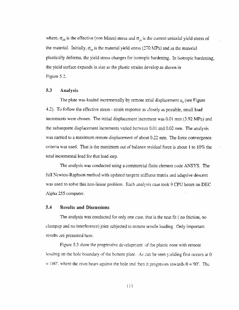
where, %t, is the effective (von Mises) stress and cy;Sis the current uniaxial yield stress of
the material. Initially, _ys is the material yield stress (270 MPa) and as the material
plastically deforms, the yield stress changes for isotropic hardening. In isotropic hardening,
the yield surface expands in size as the plastic strains develop as shown in
Figure 5.2.
5.3 Analysis
The plate was loaded incrementally by remote axial displacement Uo (see Figure
4.2). To follow the effective stress - strain response as closely as possible, small load
increments were chosen. The initial displacement increment was 0.01 mm (3.92 MPa) and
the subsequent displacement increments varied be_veen 0.01 and 0.02 ram. The analysis
was carried to a maximum remote displacement of about 0.22 turn. The force convergence
criteria was used. That is the maximum out of balance residual force is about 1 to 10% the
total incremental load for that load step.
The analysis was conducted using a commercial finite element code ANSYS. The
full Newton-Raphson method with updated tangent stiffness matrix and adaptive descent
was used to solve this non-linear problem. Each analysis case took 9 CPU hours on DEC
Alpha 255 computer.
5.4 Results and Discussions
The analysis was conducted for only one case. that is the neat fit ( no friction, no
clampup and no interference) joint subjected to remote tensile loading. Only important
results are presented here.
Figure 5.3 show the progressive development of the plastic zone with remote
loading on the hole boundary of the bottom plate. As can be seen yielding first occurs at 0
= 180", where the rivet bears against the hole and :hen it progresses towards 0 = 90 °. Tile
1ii
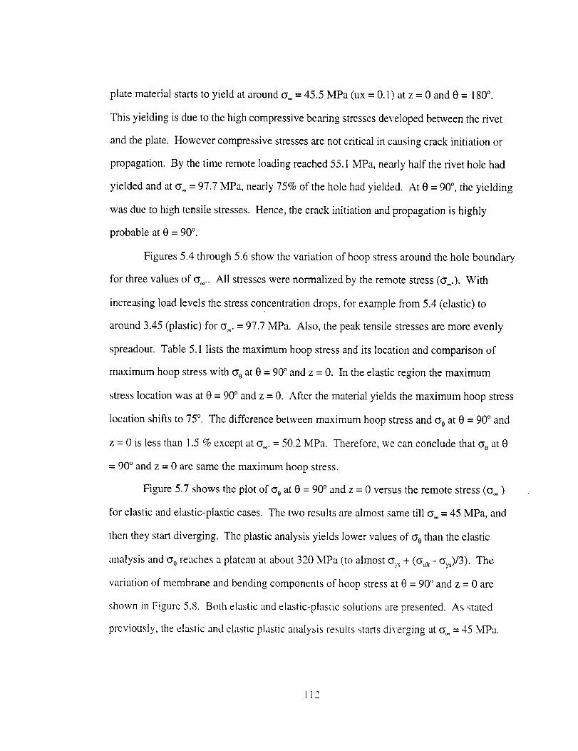
platematerialstartsto yieldat around(_ = 45.5MPa(ux = 0.1)atz = 0 and0 = 180 °,
This yielding is due to the high compressive bearing stresses developed between the rivet
and the plate. However compressive stresses are not critical in causing crack initiation or
propagation. By the time remote loading reached 55.1 MPa, nearly half the rivet hole had
yielded and at cr = 97.7 MPa, nearly 75% of the hole had yielded. At 0 = 90 °, the yielding
was due to high tensile stresses. Hence, the crack initiation and propagation is highly
probable at t3 = 90 °.
Figures 5.4 through 5.6 show the variation of hoop stress around the hole boundary
for three values of _.. All stresses were normalized by the remote stress (cy .). With
increasing load levels the stress concentration drops, for example from 5.4 (elastic) to
around 3.45 (plastic) for or.. = 97.7 MPa. Also, the peak tensile stresses are more evenly
spreadout. Table 5.1 lists the maximum hoop stress and its location and comparison of
maximum hoop stress with cyeat e = 90' and z = 0. In the elastic region the maximum
stress location was at t3 = 90 ° and z - 0. After the material yields the maximum hoop stress
location shifts to 75 °. The difference between maximum hoop stress and _e at 0 = 90 ° and
z = 0 is less than 1.5 % except at cy. = 50.2 MPa. Therefore, we can conclude that (_e at 0
= 90 ° and z = 0 are same the maximum hoop stress.
Figure 5.7 shows the plot of cy0 at e = 90 ° and z = 0 versus the remote stress (cy=)
for elastic and elastic-plastic cases. The two results are almost same till cy = 45 MPa, and
then they start diverging. The plastic analysis yields lower values of _e than the elastic
analysis and cy0 reaches a plateau at about 320 MPa (to almost cY:s+ (_u_, - O'ys)/3)" The
variation of membrane and bending components of hoop stress at 0 = 90 ° and z = 0 are
shown in Figure 5.8. Both elastic and elastic-plastic solutions are presented. As stated
previously, the elastic and elastic plastic analysis results starts diverging at c= = 45 MPa.
112
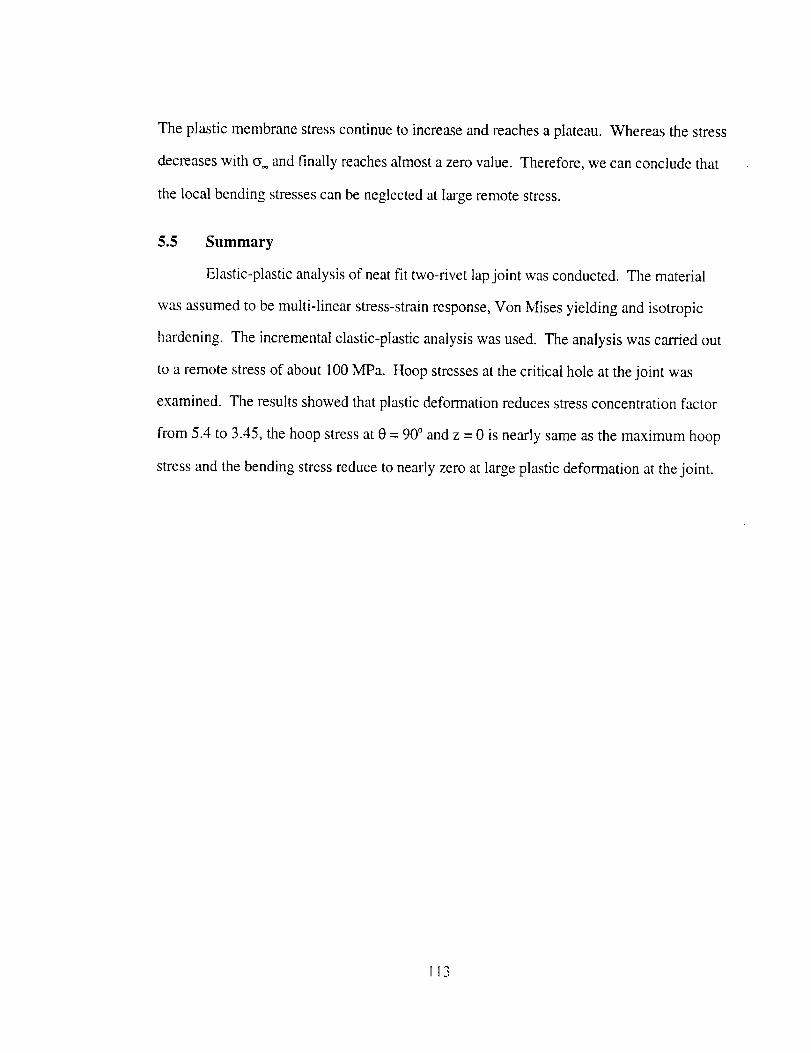
Theplasticmembranestresscontinueto increaseandreachesaplateau.Whereasthestress
decreaseswith _ andfinally reachesalmostazerovalue.Therefore,wecanconcludethat
thelocalbendingstressescanbeneglectedatlargeremotestress.
5.5 Summary
Elastic-plasticanalysisof neatfit two-rivetlapjoint wasconducted.Thematerial
wasassumedto bemulti-linearstress-strainresponse,VonMisesyieldingandisotropic
hardening.Theincrementalelastic-plasticanalysiswasused.Theanalysiswascarriedout
to aremotestressof about100MPa. Hoopstressesatthecriticalholeatthejoint was
examined.Theresultsshowedthatplasticdeformationreducesstressconcentrationfactor
from 5.4to 3.45,thehoopstressat0 = 90 ° and z = 0 is nearly same as the maximum hoop
stress and the bending stress reduce to nearly zero at large plastic deformation at the joint.
I13
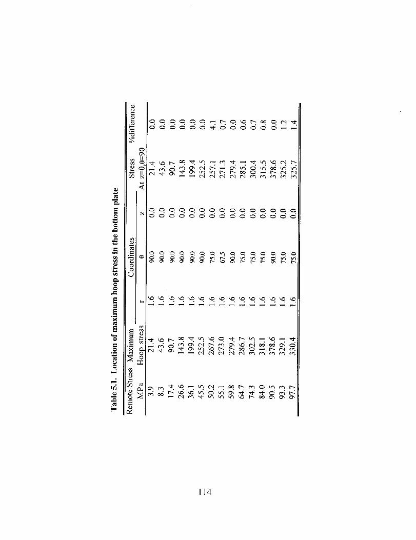
E
.Jl
r_r_
{}
i,m,
E
{}
T_
Iml
{1}{.}
l_
°_
<
N
{D
C_G
E_
_ O
r_
{1}
{D
• ° ° • . . • • • . . • ° ° .
(_ {,_ _- _) _._ lr_ {"4 _ {}_ l_ {L_ _ I.r_ ¢_ l'_
ll4
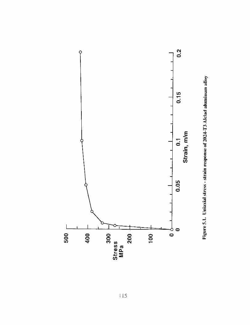
C_ Q _ C_ C_
(/)
i
n
m
m
i
m
m
i
m
c:;
L_
c:;
E
C_
wm
i,,.,4,,,J
C/)
L_0
C C_
C_
=
,m
m
u
A,,
r-
gm
L..
!
E_
m
,mu
,m
_mw
v_
L.m
omr_ill
J;5
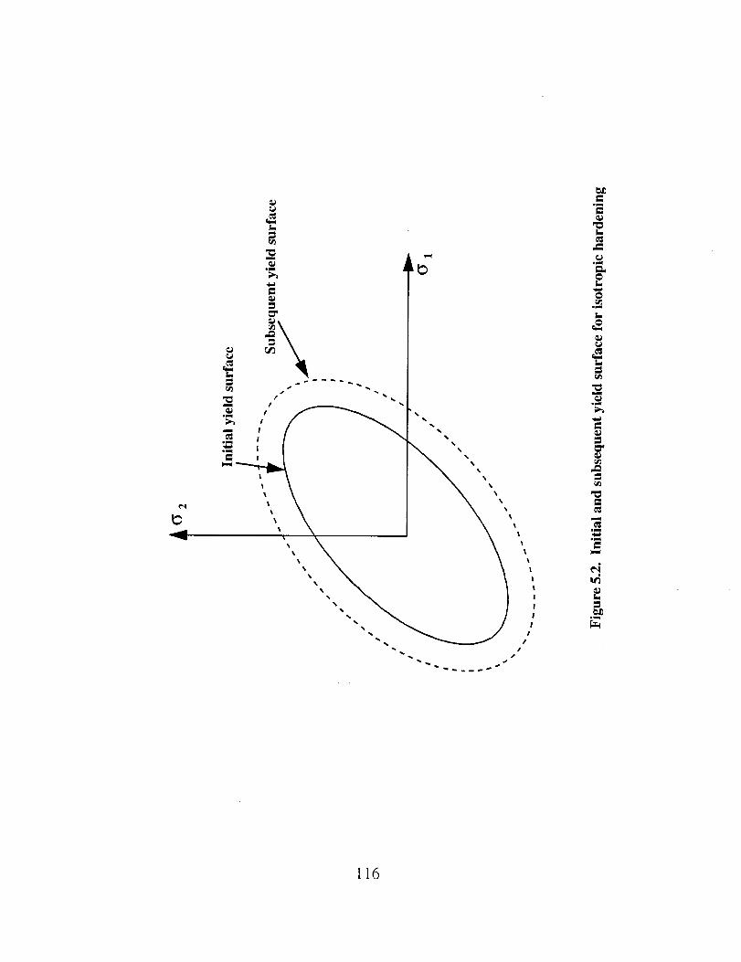
¢q
g_
,m
¢:
,ml
0
z..
¢D
h,
l
gnu
C_
U_
U_
W-q
equ_L.
.ma
g_
116
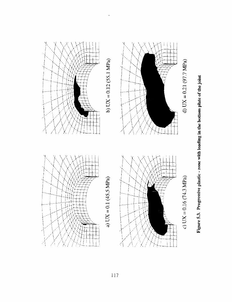
(',1
c_II
urn,
II
[.....L'-O",
O.l,5II
cm
L""-
',.0
II
@
J
@
I:
@
.i
¢=@
I
@
¢1,.,
o_
t17
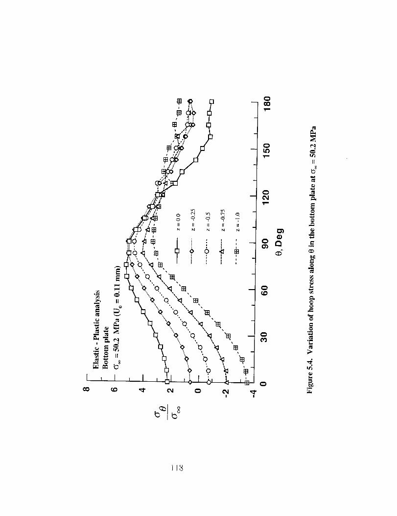
! !
It1
II8
l
m
m,
_m
b,
m..
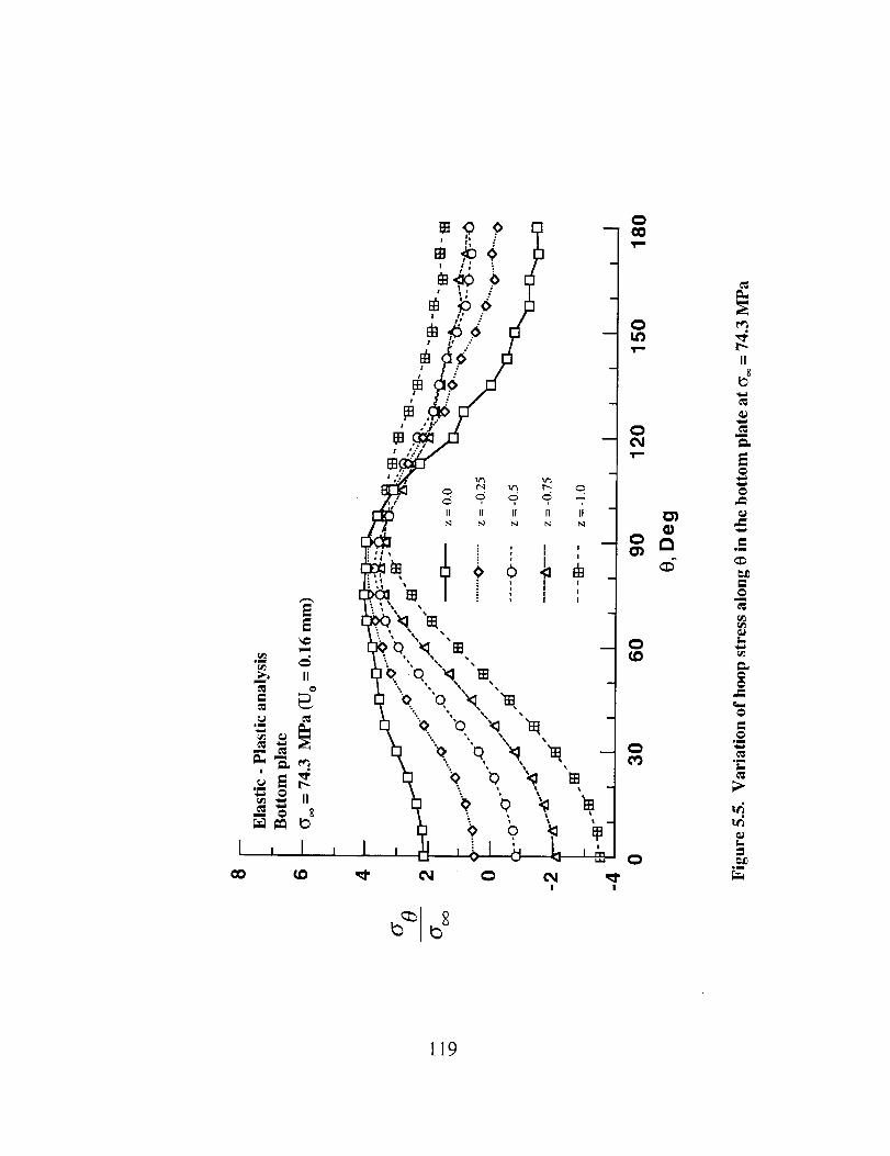
1
m
Jm
! •
*m
m
, ICD
I
r_
II
Io
J
E,,I,,,)
gm
I,.,
Im
IWz.._
I...
I19
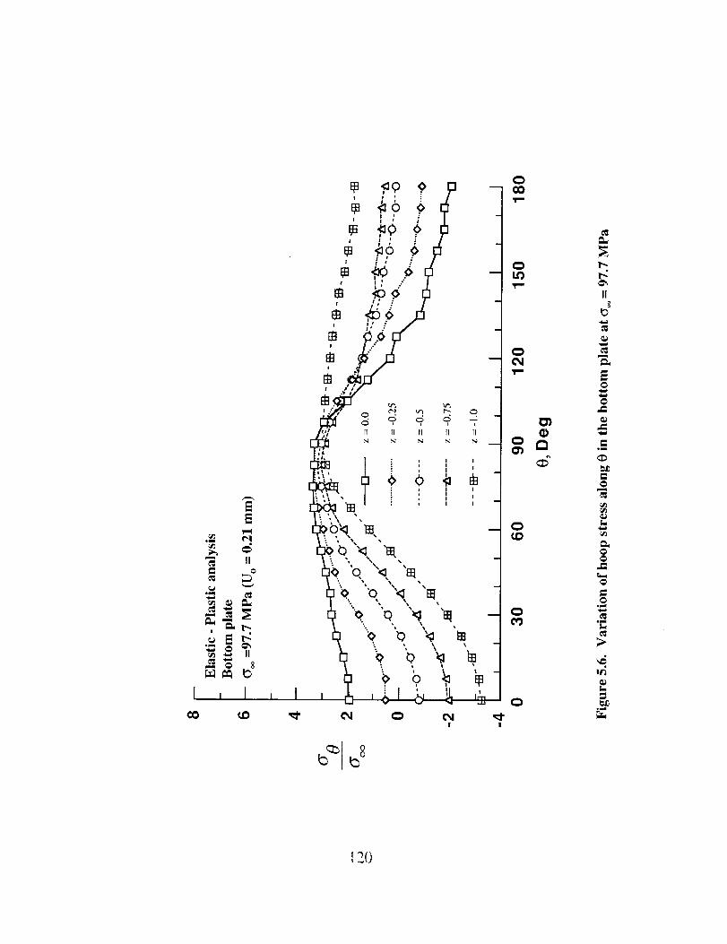
I
_0
°_
m
i
i I I
!
I I
0
0
0
0
II
i
E
_es
tip
120
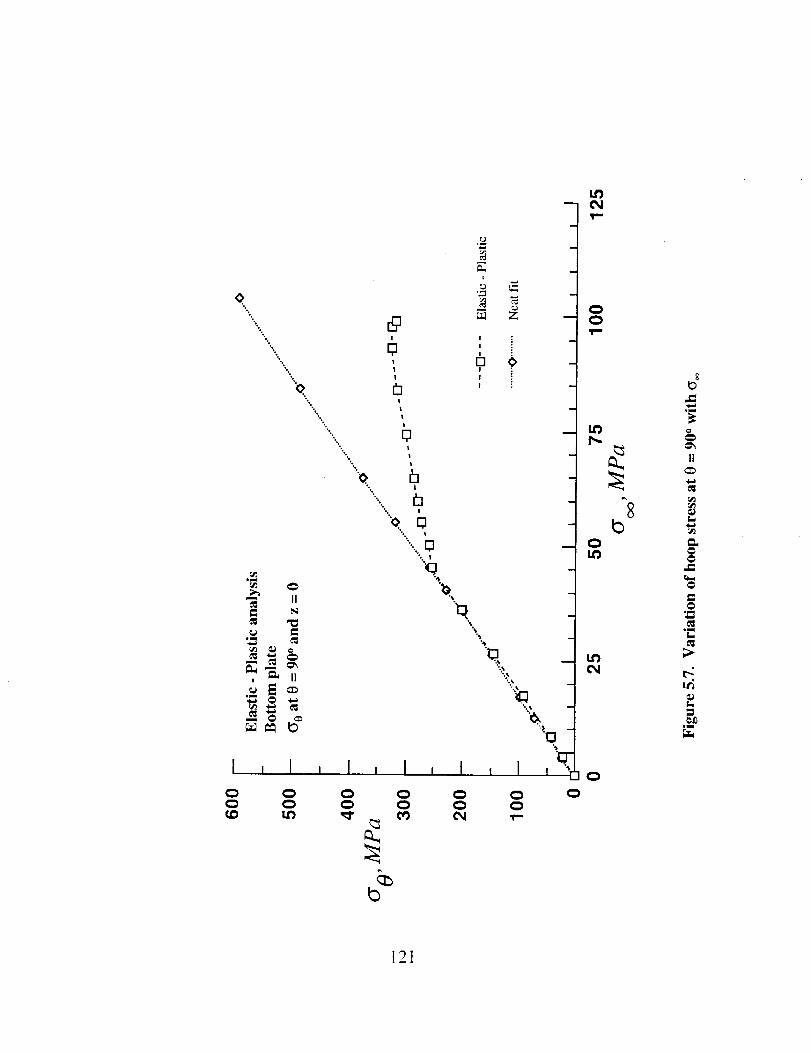
0
_:'\;
''',,,, !
'-....
°. t
m IIN
o_mv
!
I I 1 , 10 0
, I00
"....,_
, I
0
!
I
!
!
U
Z
0
1
m
q
II
L=,
°m
elI,,,
_m
121
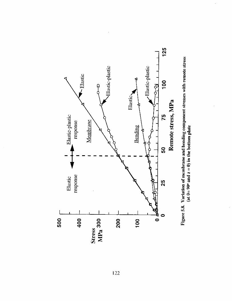
, l , I
In
o
,D
E II
°_ _'_
11
L.
o_
122
6. CONCLUDING REMARKS
Conducted a detailed stress analysis of pin joint and two-rivet single lap joint.
These joint configurations are representative of lap-splice joints used in aircraft. The lap
joint includes the load eccentricity effect where as the pin joint does not include this effect.
The analysis included the effect of plate-rivet surface-to-surface friction, rivet clampup, and
rivet interference effects. The analysis was conducted using 3-D, 8-noded isoparametric
finite elements. The contact was modeled by 5-noded surface-to-surface contact elements.
This element had capability of developing contact and separation between predetermined
surfaces. Simple rivet contraction and expansion models were developed and used to
simulate rivet clampup and interference. The range of clampup force used was 0 to 35%
rivet yield load; rivet interference used was 12.5 to 38.1 t-tin and the friction varied from 0.0
to 0.8. A commercial finite element code was used for the analysis of the joints. Elastic
analysis was conducted on the pin joint and elastic and elastic-plastic analysis were
conducted on two-rivet single lap joint. The primary focus of results analysis was on hoop
and radial contact stresses at the hole boundary. Results of this study yielded following
conclusions.
Elastic Analysis of Two-Rivet Joint
Pin Joint
(1)
(2)
Maximum stress was the hoop stress on the hole boundary and occurred at
90 ° to the load axis. The hoop stress was maximum at mid-thickness of the
plate.
The contact angle was found to be nearly 1800 .
t23
(3)
(4)
(5)
(6)
Elastic friction had negligible effect on local stresses (hoop) and hence it can
be ignored.
Clampup effect was dominant at low applied loads. Clampup decreases the
local hoop stresses. But at high applied loads, clampup effect is small.
Interference was a major factor that impacted the local stresses (hoop stress)
around the rivet hole. Interference introduces local tensile hoop stress at the
rivet hole. This initial stress reduces the rate of increase of local stresses
with remote loads. This causes the local hoop stresses to be lower than the
neat fit results at high load levels.
Contact, friction and rivet clampup nonlinearities were confined to low axial
loads. At high loads, the response is nearly linear.
Two-Rivet Lap Joint
(1) For the neat fit case hoop stress on the hole boundary was the highest and it
occurred in the bottom plate at the interface between the top and bottom
plates at 90 ° to the load axis. The maximum stress concentration factor was
found to be 5.7. Contact nonlinearity was confined to low levels of applied
load (_.< 30 MPa). At higher applied loads the response is almost linear.
The radial stress distribution on the hole boundary can be represented by a
O"rcosine function of type -- = a cos n 0. Values of 'a' and 'n' depend
oL
on the through the thickness location on the hole boundary.
(3) Elastic friction has negligible effect on local stresses (hoop) and hence it can
be ignored.
(4) For the clampup case, again the maximum stresses occurred on the hole
boundary and in the bottom plate. The clampup force did decrease the
124
(5)
stresses at the critical location and its effect can be summarized in the form
of a simple linear equation. For 10% clampup level, maximum hoop
stress location changed from 750 at low load levels to 90 ° for high load
levels. But for 25% and 35% clampup it remains at 75 ° for almost all load
levels. The Clampup effect was confined to the region under the rivet head.
Beyond the rivet head it's effects were significantly reduced.
Interference is major factor that impacts the local stresses (hoop stress)
around the rivet hole. Interference reduces the rate of increase of local
stresses with remote loads. This causes the local lhoop) stresses to be
lower than the neat fit results at high load levels.
Elastic-Plastic Analysis of Two-Rivet Joint
Elastic-plastic analysis of neat fit two-rivet lap joint was conducted. The material
was assumed to be multi-linear stress-strain response, Von Mises yielding and isotropic
hardening. The incremental elastic-plastic analysis was conducted to a remote stress of
about 100 MPa. Hoop stresses at the critical hole at the joint was examined. The results
showed that plastic deformation reduces stress concentration factor from 5.4 to 3.45, the
hoop stress at 0 = 90 ° and z = 0 is nearly same as the maximum hoop stress and the
bending stress reduce to nearly zero at large plastic deformation at the joint.
125


