
Three Essays on Dynamic Pricing and
Resource Allocation
Nur (Ayvaz) Cavdaroglu
Submitted in partial fulfillment of the
Requirements for the degree
of Doctor of Philosophy
in the Graduate School of Arts and Sciences
COLUMBIA UNIVERSITY
2012

c©2012
Nur (Ayvaz) Cavdaroglu
All Rights Reserved
ABSTRACT
Three Essays on Dynamic Pricing and
Resource Allocation
Nur (Ayvaz) Cavdaroglu
This thesis consists of three essays that focus on different aspects of pricing
and resource allocation. We use techniques from supply chain and revenue
management, scenario-based robust optimization and game theory to study
the behavior of firms in different competitive and non-competitive settings. We
develop dynamic programming models that account for pricing and resource
allocation decisions of firms in such settings.
In Chapter 2, we focus on the resource allocation problem of a service firm,
particularly a health-care facility. We formulate a general model that is ap-
plicable to various resource allocation problems of a hospital. To this end, we
consider a system with multiple customer classes that display different reac-
tions to delays in service. By adopting a dynamic-programming approach, we
show that the optimal policy is not simple but exhibits desirable monotonicity
properties. Furthermore, we propose a simple threshold heuristic policy that
performs well in our experiments. In Chapter 3, we study a dynamic pricing
problem for a monopolist seller that operates in a setting where buyers have
market power, and where each potential sale takes the form of a bilateral nego-
tiation. We review the dynamic programming formulation of the negotiation
problem, and propose a simple and tractable deterministic “fluid” analogue
for this problem. The main emphasis of the chapter is in expanding the for-
mulation to the dynamic setting where both the buyer and seller have limited
prior information on their counterparty valuation and their negotiation skill.
In Chapter 4, we consider the revenue maximization problem of a seller who
operates in a market where there are two types of customers; namely the “in-
vestors” and “regular-buyers”. In a two-period setting, we model and solve
the pricing game between the seller and the investors in the latter period, and
based on the solution of this game, we analyze the revenue maximization prob-
lem of the seller in the former period. Moreover, we study the effects on the
the total system profits when the seller and the investors cooperate through
a contracting mechanism rather than competing with each other; and explore
the contracting opportunities that lead to higher profits for both agents.
Contents
List of Tables v
List of Figures vii
Acknowledgement viii
Chapter 1: Introduction 1
Chapter 2: Hospital Resource Allocation Problem 5
2.1 Introduction . . . . . . . . . . . . . . . . . . . . . . . . . . . . 5
2.2 Literature Review . . . . . . . . . . . . . . . . . . . . . . . . . 8
2.3 Basic Model . . . . . . . . . . . . . . . . . . . . . . . . . . . . 12
2.3.1 The Structure of the Optimal Policy . . . . . . . . . . 15
2.3.2 Protect-Constant Policies . . . . . . . . . . . . . . . . 17
2.4 Extensions . . . . . . . . . . . . . . . . . . . . . . . . . . . . . 21
2.4.1 Time-Varying Stochastic Capacity . . . . . . . . . . . . 21
2.4.2 Rejecting Type 1 Patients . . . . . . . . . . . . . . . . 23
i
2.4.3 Multiple Elective Patient Classes . . . . . . . . . . . . 24
2.5 Conclusion . . . . . . . . . . . . . . . . . . . . . . . . . . . . . 26
Chapter 3: An Analysis of Dynamic Bilateral Price Negotiations 27
3.1 Introduction . . . . . . . . . . . . . . . . . . . . . . . . . . . . 27
3.2 1-to-1 Bilateral Negotiation Problem . . . . . . . . . . . . . . 35
3.2.1 Classical 1-to-1 Bilateral Negotiation Problem . . . . . 35
3.2.2 1-to-1 Bilateral Negotiation Problem in Uncertain Envi-
ronments . . . . . . . . . . . . . . . . . . . . . . . . . . 38
3.3 Dynamic Bilateral Negotiation Games . . . . . . . . . . . . . 41
3.3.1 The Analogy Between the Revenue Management and Bi-
lateral Negotiation Problems . . . . . . . . . . . . . . . 41
3.3.2 Fluid Formulation of the Dynamic Game . . . . . . . . 47
3.3.3 The Informed Buyers in BPP Setting . . . . . . . . . . 50
3.3.4 Dynamic Negotiation Games under Uncertainty . . . . 54
3.3.5 A Comparison of Seller Revenues in the Dynamic SPP
vs. BPP Settings . . . . . . . . . . . . . . . . . . . . . 56
3.4 Applications in Non-Stationary Environments . . . . . . . . . 59
3.5 Numerical Results . . . . . . . . . . . . . . . . . . . . . . . . . 70
3.5.1 Comparison of BPP and SPP settings . . . . . . . . . . 70
3.5.2 The Effect of the Negotiation Parameter . . . . . . . . 73
ii
3.5.3 An Analysis about the Effect of Uniform Distribution
Assumption . . . . . . . . . . . . . . . . . . . . . . . . 75
3.5.4 Stochastic Dynamic BPP Problem . . . . . . . . . . . 77
3.6 Conclusion . . . . . . . . . . . . . . . . . . . . . . . . . . . . . 80
Chapter 4: Pricing Problem of a Monopolist in the Presence of
Investors 82
4.1 Introduction and Literature Review . . . . . . . . . . . . . . . 82
4.2 The Decentralized Model . . . . . . . . . . . . . . . . . . . . . 86
4.2.1 The Pricing Problem at t = 1 . . . . . . . . . . . . . . 89
4.2.2 The Quantity-Claiming Problem at t = 0.5 . . . . . . . 96
4.2.3 The Quantity Selection Problem of Investors at t = 0 . 99
4.2.4 The Price Setting Problem of the Seller at t = 0 . . . . 100
4.3 The Centralized Model . . . . . . . . . . . . . . . . . . . . . . 100
4.4 The Price of Anarchy . . . . . . . . . . . . . . . . . . . . . . . 102
4.5 Numerical Analysis: Evaluating a Candidate Contracting Scheme108
4.6 Conclusion . . . . . . . . . . . . . . . . . . . . . . . . . . . . . 114
Bibliography 115
Appendix A: Appendix to Chapter 2 123
A.1 Proof of Theorem 1 . . . . . . . . . . . . . . . . . . . . . . . . 123
A.2 Proof for Section 2.4.1 . . . . . . . . . . . . . . . . . . . . . . 125
iii
A.3 Proof for Section 2.4.2 . . . . . . . . . . . . . . . . . . . . . . 128
A.4 Proof for Section 2.4.3 . . . . . . . . . . . . . . . . . . . . . . 129
Appendix B: Appendix to Chapter 3 133
B.1 Proof of Theorem 3 . . . . . . . . . . . . . . . . . . . . . . . . 133
B.2 Analysis of the One-to-one Negotiation Problem between an
Informed and Uninformed Agent . . . . . . . . . . . . . . . . 135
B.3 Proof of Theorem 6 . . . . . . . . . . . . . . . . . . . . . . . . 137
B.4 Proof of Proposition 3 . . . . . . . . . . . . . . . . . . . . . . 140
Appendix C: Appendix to Chapter 4 142
C.1 Proof of Proposition 4 . . . . . . . . . . . . . . . . . . . . . . 142
C.2 Proof of Proposition 5 . . . . . . . . . . . . . . . . . . . . . . 143
C.3 Proof of Proposition 7 . . . . . . . . . . . . . . . . . . . . . . 150
iv
List of Tables
2.1 Sensitivity Analysis with Respect to the Penalty Coefficient w2. 19
2.2 Sensitivity Analysis with Respect to the Capacity C. . . . . . 19
2.3 Sensitivity Analysis with Respect to the Time Horizon T . . . 19
2.4 Sensitivity Analysis with Respect to the Type-1 Patient ArrivalRate l1 . . . . . . . . . . . . . . . . . . . . . . . . . . . . . . . 20
2.5 Sensitivity Analysis with Respect to the Type-2 Patient ArrivalRate l2. . . . . . . . . . . . . . . . . . . . . . . . . . . . . . . 20
3.1 BPP vs. SPP under various C values . . . . . . . . . . . . . . 71
3.2 BPP vs. SPP under various vs values . . . . . . . . . . . . . . 72
3.3 The Ratio of Seller Revenues under Uniform Distribution As-sumption to the Revenues in Full Information Setting . . . . . 76
3.4 The Ratio of Seller Revenues under Uniform Distribution As-sumption to the Revenues in Full Information Setting . . . . . 76
3.5 Changing vs . . . . . . . . . . . . . . . . . . . . . . . . . . . . 78
3.6 Changing C . . . . . . . . . . . . . . . . . . . . . . . . . . . . 78
3.7 Changing d . . . . . . . . . . . . . . . . . . . . . . . . . . . . 79
v
3.8 Changing N . . . . . . . . . . . . . . . . . . . . . . . . . . . . 79
4.1 Performances of Various Contracting Schemes (changingK1 andthe ratio ps,new0 /pc0) . . . . . . . . . . . . . . . . . . . . . . . . 112
4.2 Performances of Various Contracting Schemes (changingK0 andthe ratio ps,new0 /pc0) . . . . . . . . . . . . . . . . . . . . . . . . 112
4.3 Different Problem Settings . . . . . . . . . . . . . . . . . . . . 114
vi
List of Figures
2.1 Optimal Protection Levels for Each Capacity Level . . . . . . 21
3.1 Examples of Parameter Paths . . . . . . . . . . . . . . . . . . 61
3.2 Seller revenues (as a percentage of revenue at k = 0) for variousk and C values . . . . . . . . . . . . . . . . . . . . . . . . . . 74
4.1 Sequence of Events . . . . . . . . . . . . . . . . . . . . . . . . 90
4.2 Regions of Equivalence (4.8) . . . . . . . . . . . . . . . . . . . 95
4.3 Regions of Equivalence (4.16) . . . . . . . . . . . . . . . . . . 103
vii

Acknowledgement
I consider myself as a very lucky person: I was born into a wonderful family,
was endowed with “sufficient” amount of beauty, intelligence and personal
traits, but most importantly, have always met wonderful people all my life. In
fact, implicating the “valuable” people in my life has always been my motto:
People who influenced me, people who inspired me. This note is a tribute to
all of them.
Murat Koksalan, my professor in METU, is the first person to introduce me to
scholarly work and ensured me to pursue higher education. Another professor
from my college, Sedef Meral, is the person who led me to apply to Columbia
University. I am very much indebted to both of them, and all my other
Professors from IEOR department of METU, for being able to write these
words at the moment.
In the last six years, I have been extremely lucky to work with some of the
best people I could hope to learn from. When I was perhaps in the darkest
days of my life, Soulaymane Kachani welcomed me by accepting to be my
advisor, always supported me with his kind personality and directed me with
his excellent leadership, for which I am extremely grateful. By accepting to co-
advise me, Costis Maglaras shared his research genius, his broad experiences
and his valuable time with me. Woonghee Tim Huh is another person I am
much indebted: Without his support, I would not have published my first
paper. This work would have never been possible without their support and
guidance. I am truly honored to have had this opportunity to work so closely
with such brilliant researchers. Their perpetual energy and enthusiasm in
research always motivated me. I am eternally grateful for all the time and
viii

effort they have put in over the years to cultivate my knowledge and skills.
Besides my advisors, I would also like to thank the members of my PhD thesis
committee - Garud Iyengar and Vineet Goyal, for their valuable time.
To Ali Sadighian, I owe a lot: Without his support, I could not have completed
this thesis. He has been a helping hand and a caring friend.
Ph.D education is usually thought of as taking the necessary classes, spend-
ing hours in front of the computer, and meeting your advisor to discuss the
progress of the research. But it is much more than that: It is a truly trans-
forming experience. It transforms you from an inexperienced student who has
merely reached the side of the ocean of wisdom to a person who has had the
chance to taste a few drops of it. The path of pursuing a Ph.D degree is the
first step to delve into the depths of this endless ocean; which, to a person
who tasted a few drops of this enchanted potion, is then inevitable. You begin
repeating the famous words of Samuel Beckett to yourself: “Ever tried. Ever
failed. No matter. Try again. Fail again. Fail better.” And Ph.D education
is also a matchless adventure that allows you to share your laughter and your
tears with your comrades that come from all parts of the world and incidentally
been assigned to the same office with you: My dear office mates from Mudd
Building Room 313-A and CEPSR Building Room 821 have both helped me
with the ideas in terms of research, and also let me have wonderful memories
of the office life. I am truly thankful to all, and in particular, Vijay Desai and
Serhat Aybat, who made me feel at home and gave me a lot of good advice
at different stages of my research; Ummuhan Akbay, who was my roommate
besides being my friend in research; and Ozge Sahin and Serkan Eren, who
were both my friends and my seniors, helping me to get settled in a foreign
country.
ix

My sincere thanks also go to Ward Whitt, Cliff Stein, Daniel Bienstock, Martin
Haugh, Jay Sethuraman, Alp Muharremoglu, and other members of the IEOR
(and DRO) faculty for all their advice and support over the years. I am also
indebted to the staff at the department for their continued support, especially
Donella Alanwick, Risa Cho, Jaya Mohanty and Michael Mostow.
My life as a Ph.D. student at Columbia was enriched by the company of
the great friends I found here. I have some of my best life-long memories
from the parties, conversations, and other activities that I enjoyed in the
company of Arseniy, Caner, Cecilia, Damla, Denis, Deniz, Emre, John, Jae-
Hyun, Kun-Soo, Lin, Masoud, Matulya, Ohad, Rishi, Rodrigo, Rouba, Ruxian,
Sabri, Sercan, Sekip, Shyam, Tony, Tulia, Yixi, Yori, Yunan, Xianhua, Xingbo,
Zongjian and many others that I cannot do justice in this short note.
Sila (Saylak) and Tansel (Alan), who have been my friends since high school,
are my saviors: They opened the doors of their house whenever I needed a
place to stay. (Thank you very much guys! I love you!)
And my family: My father, who was born into a poor family, and climbed his
way up to being a Biology Professor and the dean of Science and Literature
Faculty of one of the best universities in Turkey. He is my role model, he is my
hero. My mother encouraged me to do my best all the time, and was always
there for me with all her warmness and unwavering love. They say that “A
person whose mother is alive is never alone in the world”, and that is so true.
I am so grateful for having her as my mother. And my sister: She is my little
princess, my best friend, and the person who showed me there were always
other possible ways. Hilal, without you, I would become a very boring and
reserved person; thank you for emancipating me from my small nest!
x

Finally, my beloved husband Burak: If I had believed in reincarnation, I would
think that I must have saved a country in my previous life to be blessed to find
you: You endured all my sulkiness and moodiness whenever things went bad
in research, you always encouraged me to do my best, you were a helping hand
at home and at work, and made the last three years of my life very enjoyable
and most unforgettable. You are the most wonderful husband a woman could
want. Thank you my dear, and always be by my side till death us do part. I
love you.
xi

To my mother, To my father
xii
1
Chapter 1
Introduction
This thesis consists of three essays that utilize various methods of dynamic
optimization, revenue management and pricing literature, and game theory to
solve problems in the area of pricing and resource allocation. We use techniques
from dynamic programming, scenario-based robust optimization and game
theory to derive optimal pricing and resource allocation polices.
Allocation of resources among various customer groups or customers arriving
at various time points along the sales horizon has been a fundamental prob-
lem of production and service firms throughout the history. This problem has
elicited interest from various researchers from different fields, and even led to
“yield management” to emerge as an independent research field. The revenue
loss stemming from unwise pricing practices and inefficient resource allocation
schemes can have substantial effects on the profitability of the firms, as well
as the social welfare of the society. Hence, many researchers and practition-
ers have developed sophisticated models of revenue management and resource
2
allocation to address this problem.
Despite the fact that the airline industry was the very first industry which
took advantage of dynamic pricing and revenue management techniques, re-
cently many other business sectors are willing to invest in and investigate the
potential benefits of revenue management and dynamic pricing. In this thesis
also, we start with the application of revenue and supply chain management
techniques in a non-conventional area, namely “health care”. To this end,
we first focus on the resource allocation problem of a service firm, particu-
larly a health-care facility in Chapter 2. We formulate a general model that
is applicable to various resource allocation problems of a hospital. We con-
sider a system with multiple customer classes that display different reactions
to the delays in service. By adopting a dynamic-programming approach, we
show that the optimal policy is not simple but exhibits desirable monotonic-
ity properties. Furthermore, we propose a simple threshold heuristic policy
that performs well in our experiments. Finally, we conclude the chapter by
discussing various extensions of the model to extend the applicability of the
results across several real-life problems.
Another non-conventional area for the application of pricing and revenue man-
agement techniques is the “real-estate”. In Chapter 3, motivated by the rev-
enue maximization problem of a real estate developer, we turn our attention
to finding the best dynamic pricing strategy for a monopolist seller that op-
erates in a setting where buyers have market power and each potential sale
takes the form of a bilateral negotiation. This problem is again connected to
the problem of the previous chapter, especially considering the fact that the
revenue management of a monopolist seller that operates in a setting where
buyers have market power is essentially a capacity allocation problem. In this
3
setting, buyers arrive sequentially over time and negotiate separately with the
seller to purchase one unit of the offered good. The outcome of each such ne-
gotiation depends on the valuations of the seller and the buyer for that good,
their relative negotiation power, as well as their beliefs for the other party’s
valuation. We review the dynamic negotiation problem, and propose a simple
and tractable deterministic “fluid” analogue for this problem. The main em-
phasis of the chapter is in expanding the above formulation to the case where
both the buyer and seller have limited prior information on their counterparty
valuation and their negotiation skill, and mainly analyze the sales process in
a dynamic setting. Our first result shows that if both the seller and buyer are
bidding so as to minimize their maximum regret over possible counterparty
valuation distributions, then it is optimal for them to bid as if the unknown
valuation distributions were uniform. Building on this result and the fluid
formulation of the dynamic negotiation problem, we characterize the seller’s
optimal reserve price, i.e., the minimum price that she should be willing to
accept for one unit of the good at any given point in time. Finally, we expand
on the above ideas to formulate and study the seller’s problem in the case
where the primitives of the buyer valuation distributions are unknown and
non-stationary using ideas from scenario-based robust optimization. Despite
the fact that the motivating application is from residential real-estate, the
model and proposed approach are generally applicable. This analysis forms
and completes Chapter 3.
Finally, motivated by our work in Chapter 3, we consider the problem of a
real estate developer from a different angle: In Chapter 3, we were mainly
concerned with “naive” buyers who do not strategize over purchase decision
or invest in the real estate with the intention of obtaining profit from their
4
investment. However, in practice, despite being a rather non-liquid investment
instrument, real estate investment is one of the items investors include in their
portfolio: It is common for investors to own multiple pieces of real estate, one
of which serves as a primary residence, while the others are used to generate
rental income and profits through price appreciation. Hence, in Chapter 4,
we consider the revenue maximization problem of a seller who operates in
a market where there are two types of customers; namely the “investors”
and “regular-buyers”. The regular buyers are similar to the naive buyers of
the previous chapter; however the investors purchase the units to resell them
later, thus creating a competition against the seller in the latter period of
the sales horizon. In a setting that is comprised of two sales periods, we
first model and solve the pricing game between the seller and the investors in
the latter period, and based on the solution of this problem, we formulate the
revenue maximization problem of the seller in the former period. Moreover, we
analyze how the total system profits increase when the seller and the investors
cooperate through a contracting mechanism rather than competing with each
other. Again, the problem takes its roots from the real estate industry, however
the results are generally applicable in any duopoly setting with non-flexible
capacities.

5
Chapter 2
Hospital Resource Allocation
Problem
2.1 Introduction
In this chapter, we study the problem of dynamically allocating a single re-
source of fixed capacity to several customer streams. The demand of some
customer types can be fully backlogged whereas other demand will be lost if
not fulfilled immediately upon arrival. While this kind of a situation arises in
many industries, our motivation to study this problem comes from the exis-
tence of various patient types in a health-care facility. Some of these patients
are of critical condition, or may require immediate attention. Other patients
may not require immediate treatment, but the monetary benefits they would
bring may be higher than that of the first type of patients. An example is the
allocation of operating rooms to emergency and elective surgical operations.
6
If both cases arrive at the hospital at the same time, the humanitarian (and
reputational) concerns favor the admission of the emergency case first. But
when the number of emergency patients to arrive during the course of the day
is unknown, how a manager should plan the operating room utilization sched-
ule remains to be an unanswered question. In short, in an environment with
rising costs and increasing competition, the managers of a health-care facility
need to contend with humanitarian versus monetary conflicts, and thus, have
to address the tradeoffs arising from this kind of a resource allocation prob-
lem. The quality of the provided health care and the monetary aspects of the
problem are often interwoven, yielding an even more delicate situation that
needs to be handled with utmost care.
In many health-care facilities, the resource allocation problem is considered
as being too complicated, and in general, some rule-of-thumb approaches are
employed. For instance, in many institutions, a senior floor nurse is entrusted
with the process of allocating hospital beds to the patients waiting in the
system, the rationale being that this person has the required experience and
the knowledge to judge the urgency of the cases. However, this kind of inexact
approaches could lead to substantial inefficiencies in terms of social benefits
and/or monetary gains to be obtained had an analytical solution methodology
been employed (e.g. see Patrick and Puterman (2007) for an example).
Nevertheless, there exist several papers in the literature that analyze the re-
source allocation problem of a health-care facility using various techniques
ranging from queuing to simulation models, optimization, and dynamic pro-
gramming formulations. For instance Gerchak et al. (1996) focus on the
operating rooms’ capacity utilization; Green et al. (2006) deal with the effec-
tive utilization problem of an MRI center; and starting with Young (1962), a
7
number of authors focus on the allocation of hospital beds to various patient
classes. Instead of focusing on the details of some specific resource within an
hospital, our work provides an abstract and more general framework for un-
derstanding different behavior patterns of various patient classes in terms of
their reaction to delays in the service. Our intention is to look for an over-
arching guideline and intuition that can be useful for any specific resource
allocation problem. To achieve this goal, we use a dynamic programming ap-
proach which is common in the inventory management literature. We observe
that, under certain modeling assumptions, there are similarities between the
resource allocation problem of a hospital and the capacity allocation problem
of a manufacturing firm that serves multiple types of customers.
Throughout the article, we will focus on the problem of managing the admis-
sions of stochastically arriving patients in an hospital and build our model
upon this terminology. However, the reader should note that the derived in-
sights are applicable to various resource management problems of service firms
with multiple customer types displaying different reactions to possible delays
in service (i.e., lost sales versus backorders).
This chapter is organized as follows. Section 2.2 describes the related liter-
ature, which spans revenue management, supply chain and inventory man-
agement, as well as several methodologies used in the context of resource
allocation in health-care facilities. In section 2.3, we present our model and
a dynamic programming formulation. We then prove that the optimal policy
has desirable monotonicity properties. While the optimal policy is not simple,
we propose a simple threshold-type policy that performs well in our numerical
experiments. In section 2.4, we consider several extensions of the model that
include features that arise in practice. Finally, in section 2.5, we summarize

8
our work and present avenues for future research.
2.2 Literature Review
Since our work is in the context of health care, we first review the existing
literature on the resource allocation problem of a health-care facility. Then,
we will review relevant papers on general production-service systems that face
demands from multiple customer types.
Health-Care Management Literature. The patient admission problem
of a health-care facility has been studied by several researchers, mostly using
the tools of simulation or queuing theory. Most of the papers to our knowledge
focus on deriving the best “cut-off”-type of policy – which allows for the ad-
mission of the ‘less serious’ patients after a critical number of beds are reserved
for the ‘critical’ patients whose arrival process is stochastic. The classic work
of Young (1962) is the first to represent the hospital admissions scheduling
as a queuing model. Kolesar (1970) uses Markovian decision models; while
Esogbue and Singh (1976) shed more light onto the problem by finding the
optimal threshold levels under a linear cost structure. Huang (1995) is able
to come up with the number of beds that are required for different days of the
week by using a Monte-Carlo simulation model.
Along with queuing models, there are other mathematical modeling approaches
to address resource allocation in a health-care facility. A number of decision
support systems have been developed with the purpose of helping hospital
managers in the bed-allocation decision. The work of McClean and Millard
(1995), and that of Mackay (2001) depicting the implementation process of
two decision support systems in the South Australian public hospital system
9
are two examples of this line of research. Although the results depend heavily
on the distribution of the underlying data or system stability, these meth-
ods are proven to be useful in resource allocation management. Regarding
other mathematical modeling approaches, Dantzig (1969) is first to develop a
scheduling system using a linear programming formulation under deterministic
parameters. His work represents the first attempt to use an objective function
that explicitly incorporates certain cost elements; in particular, the penalty
cost. Later, Harper and Shahani (2002) develop a detailed simulation model
in the light of bed occupancies and refusal rate, and Ruth (1981) uses a mixed
integer programming formulation to match the demand with the hospital ser-
vices. For a comprehensive analysis and the summary of the research on this
topic, we refer the reader to Milsum et al. (1973) and Smith-Daniels et al.
(1988)
Most of these models, however, suffer from strong assumptions that restrict
their use. The queuing models assume that the service time (the occupancy
time of a bed) and the interarrival times are exponentially distributed, which
may not always hold in practice. In fact, Young (1962) tested the use of his
queuing model against the results of a simulation model and found that sig-
nificantly different results were obtained by the two techniques. Similarly, the
steady-state Markovian models are criticized regarding their attempt to ap-
ply a Markov decision model to a problem that is essentially non-Markovian,
which amounts to an oversimplification of the system dynamics. Other models
also suffer from oversimplification issues such as the deterministic assumptions
(e.g. Dantzig (1969)). In this paper, we adopt a dynamic programming ap-
proach which allows modeling the non-stationary stochastic arrival pattern of
patients.
10
Production/Service Systems. Both queuing and dynamic programming
models have been widely used in inventory, service and other related areas
involving resource allocation problems. Our problem shares some similarities
with the problem of selling a single product to multiple customer classes under
uncertain arrivals. The early work of Topkis (1968) considers the rationing of
inventory to demand from multiple customer classes and shows that a base-
stock policy is optimal; our setting differs from this and other inventory models
since the amount of capacity available at a health-care facility in a period is
fixed and cannot be stored. Duenyas (2000) formulates the problem as a semi-
Markov decision process and examines the “due date setting policy” – his
work is grounded on the assumption that the manufacturer can sequence the
orders in any desired manner, which is clearly not applicable in our context
due to the ethical and legal issue of patient rights. Carr and Duenyas (2000)
address the admission control and sequencing in a production system with two
product classes, and they use a simple two-class M/M/1 queue and come up
with optimal switching curves. Maglaras and Zeevi (2005) also use a queueing
framework with stationary demand to model two types of demand – these two
types are distinguished based on whether the customer receives guaranteed
service or “best-effort” service (served only when the server is not too busy),
similar to our distinction of customer types.
An interesting work of Carr and Lovejoy (2000) focuses on determining the
optimal portfolio of multiple customer segments for a capacitated firm; in this
model, however, the demand should remain stationary once the portfolio is
calculated.
Gupta and Wang (2006) consider a similar problem of allocating production
capacity between two classes of demand, and show the optimality of a policy
11
based on critical numbers. Other important papers involving a single-item,
make-to-stock production system with multiple demand classes are papers
of Ha (1997a,b) and the work of Sobel and Zhang (2001). Finally, Ding et al.
(2006) analyze the tactical problem of allocating inventory to several customer
classes when partial backlogging is possible, and they maximize revenue by
dynamic pricing through customer discounts where the probability of a denied
customer to remain in the system is based on the discount offered to her. This
dynamic pricing approach forms the principal difference of their work from
ours, as tweaking with prices is not readily acceptable in health-care settings.
In all of the papers mentioned above (except for that of Ding et al. (2006)),
the unsatisfied demand is either entirely backlogged or completely lost, but
not both. Even though in practice it is quite reasonable that some unsatisfied
demand can be backlogged while other demand is lost, there exist only a
few papers in the inventory literature that model multiple demand classes of
customers based on the stock-out behavior.
Of these, Duran et al. (2008) consider a system with two demand classes,
where demand coming from one of these classes is immediately lost if unful-
filled; and the unsatisfied demand of the other class is backlogged for one
period. Tang et al. (2007) address a two-class model where higher priority
is given to the backorder demand, and the lost-sales demand class is served
later. Both papers show the optimality of base-stock, or modified base-stock
policies. The paper of Zhou and Zhao (2010) differs from the previous two
by involving the assumption that previous backorders can be satisfied in any
future period (not necessarily in the immediate next period), and showing that
in that setting base-stock policies may no longer be optimal. The main result
of this paper is to show that the optimal policy satisfies some monotonicity
12
properties. The main difference of our work from the mentioned papers lies in
the different characteristics of inventory and service settings – the manager of
an inventory system has the flexibility to decide on the number of units to be
ordered in each period and, furthermore, these units can be stored for future
use, but in our system only a fixed amount of capacity becomes available in
each decision epoch. Hence, our work speaks to one of the basic questions in
revenue management: how to make the best use of a limited capacity through
allocation.
In summary, we use dynamic programming formulation, as common in the
inventory-related literature, to study the dynamic capacity allocation problem
in a service context when multiple types of customers are present and the
underlying demand pattern may not be stationary. Thus, our model is related
to two bodies of literature: the resource allocation problem of the service
industries (particularly, the health-care facilities) and the inventory control
problem of manufacturing systems with both lost-sales and backorders. In this
work, we uncover insights into how the optimal policy behaves, and propose a
simple heuristic policy that performs well.
2.3 Basic Model
We consider a system with two patient groups, whom we will refer to as type
1 and type 2 patients. These patient types are distinguished by their behavior
upon arrival at the hospital. Type 1 patients wait in the system until they
receive service while type 2 patients leave the system (i.e., are “lost”) if they
cannot be accommodated immediately upon arrival. The modeling of type 1
and type 2 patients is motivated by elective surgery patients and emergency
13
patients. The elective surgery patients require a surgical operation that is
not urgent and they are willing to wait in the system until the necessary
resources become available for their treatment (e.g., certain types of plastic
surgery patients). By contrast, emergency patients arrive at the hospital in
critical condition, and they should either be admitted immediately or be sent
to another facility in close proximity.
If a type 2 patient cannot be accommodated immediately, this patient is lost
to the system incurring a goodwill penalty of w2 > 0. This penalty cost
represents the possibly worsening condition of the patient during his transfer
to a nearby facility or damage to the hospital’s reputation. Meanwhile, a
type 1 patient will wait in the system until she is treated while incurring a
goodwill penalty w1 > 0 per unit time she spends awaiting treatment. This
cost represents the increasing anxiety of the patient while being enrolled in
the waiting list. We denote the expected per-patient revenue from a type 1
patient and a type 2 patient by r1 > 0 and r2 > 0, respectively. Let C denote
the capacity of the hospital per day, which is to be allotted to two patient
groups. We assume that each patient (type 1 or type 2) consumes exactly
one unit of capacity in the time period that she is admitted for treatment.
This assumption, which decouples the admission process from the treatment
stage by allowing that the system starts fresh with C units of capacity at
each new period, may not always hold in practice; but serves as a reasonable
approximation for hospital wards for which the length of stay is sufficiently
short and does not vary much; or for some specific resources of the hospital (for
example, interpret C as the capacity of a certain test required for all newly-
admitted patients). In this work, we do not explicitly model the length-of-stay
distributions in order to avoid that available capacity depends on the history of
14
patient arrivals; the queuing-based framework would model the length-of-stay
feature more appropriately. However, our model and findings can be extended
to the case of stochastic and non-identical capacity (section 2.4), which can
approximately account for the effect of a patient occupying one unit of resource
for several periods.
In each period, we assume that the following sequence of events takes place: At
the beginning of each period (for instance, a day) t, the hospital management
observes the number of backlogged patients st, and based on this observation,
decides how many backlogged type 1 patients to admit in the current period
(while the rest of the unaquitted type 1 patients remain backlogged). (In sec-
tion 2.4, we allow the manager to reject some type 1 patients.) The remaining
capacity will be protected for type 2 patients who arrive throughout the day.
All type 1 arrivals during the course of the day will be placed on the back-
logged patients list. We assume that the number of type 1 patient arrivals
on any given period t can be approximated by a random variable Mt with a
continuous and differentiable cumulative density function (cdf) H1t with the
probability density function (pdf) h1t , and the distributions are independent
but not necessarily identical across periods over the planning horizon. Simi-
larly, type 2 arrivals in each period t is represented by a random variable Dt
with cdf H2t and pdf h2
t , and the distributions of {D1, D2, . . .} are independent.
We assume that both Mt and Dt have bounded support.
In each period t, let st ≥ 0 denote the number of backlogged type 1 patients
at the beginning of the period, and let xt ≥ 0 represent the amount of capac-
ity protected for type 2 arrivals, which is the decision made by the hospital
management. Then, the expected net revenue to be obtained in period t will
15
be given by:
L(st, xt) = r2 · E min{xt, Dt}+ r1 · E[Mt]− w1 · (st + xt − C)+
−w2 · E[Dt − xt]+ (2.1)
And the number of backlogged patients is updated by st+1 = (st−C+xt)++Mt
at the end of the period.
Note that in the above expression, the revenue from type 1 patients is collected
at the time of their arrival (which is given by the term r1 · E[Mt]) and the
penalty of backlog incurs only after they wait in the system for one period and
are still not admitted (which is given by −w1 · (st + xt −C)+). If the revenue
is instead collected at the time of service, we can account for this change by
adjusting the value of w1 to incorporate the time value of revenue. Finally, the
term r2 · E min{xt, Dt} represents the revenue collected from type 2 patients
arriving during the course of the day, and −w2 · E[Dt − xt]+ is the penalty
associated with type 2 patients who cannot be accommodated.
2.3.1 The Structure of the Optimal Policy
The following property of the single-period net revenue is useful in establishing
the structural characteristics for the optimal allocation policy. Its proof follows
easily from well-known properties of submodularity and concavity.
Lemma 1. L(st, xt) is submodular and jointly concave in its components.
We consider a planning horizon of T periods. Let α ∈ [0, 1] denote the dis-
count factor. The Bellman equation for maximizing total net revenue can be
16
formulated as follows: for 1 ≤ t ≤ T , define
ft(st) = max0≤xt≤C
[L(st, xt) + α · EMt [ft+1((st + xt − C)+ +Mt)]
], (2.2)
where the terminal condition is given by
fT+1(sT+1) = v · sT+1 ,
where v ≤ 0 is some fixed constant.
Let x∗t (st) denote the optimal amount of capacity to reserve for type 2 patients
when there are st backlogged type 1 patients in the system. If we give priority
the to backlogged type 1 patients over newly arriving type 2 patients, then
the amount of capacity available for type 2 patients would be max{C − st, 0};
thus it is easy to see that C − st is a lower bound on x∗t (st), i.e.,
st + x∗t (st) ≥ C . (2.3)
We are interested in establishing structural properties for the optimal alloca-
tion decision x∗t (·), but it turns out that the optimal decision does not follow
a simple form such as a threshold-type policy. However, we establish certain
monotonicity properties for x∗t (st). The following result shows that the amount
of capacity protected for type 2 arrivals is decreasing in the number of back-
logged type 1 patients, while the magnitude of change is at most equivalent to
the amount of variation in the number of backlogged patients.
Theorem 1. For each period t ∈ {1, . . . , T}, x∗t (st) satisfies the following
properties:
(i) x∗t (st) is decreasing in st, i.e., x∗t (st + ε) ≤ x∗t (st) for any ε > 0.
(ii) x∗t (st + ε) ≥ x∗t (st)− ε, for any ε > 0.
17
Proof: See Appendix A.1. �
The proof of Theorem 1 consists of standard arguments and is based on the
preservation of joint concavity in ft functions, from which we find the opti-
mal decision x∗t (st) based on the first-order condition (FOC). Such a partial
characterization in Theorem 1 is often the best structural result that can be
established in the inventory management and production planning models in
the literature. This is consistent with Carr and Duenyas (2000) where the
production threshold curve is monotonously decreasing in the number of type
2 orders in the production-queueing context, and also with Green et al. (2006)
where the optimal capacity allocation policy belongs to the class of monotone
“switching curve” policies in an appointment scheduling context. Such results
are useful in motivating heuristic methods as well as in computing the optimal
policy function x∗t (·).
2.3.2 Protect-Constant Policies
Since the optimal policy x∗t (·) may be difficult to find and to implement, we
focus our attention to a simpler policy which we call the protect-constant or
protect-θ policy, where θ ∈ [0, C] is a policy parameter. Under this policy, we
protect the same amount of capacity θ in each period for the type 2 patients
– unless there are more than θ units of capacity available after clearing the
backlog, in which case we make all remaining capacity available to type 2
arrivals. Mathematically,
xt(st) = max{θ, C − st} . (2.4)
While this class of policies is clearly not optimal, it is easier to define and
simpler to implement in practice compared to the optimal policy.
18
One possible method of selecting the parameter θ in the protect-constant policy
is to select the expected number of type 2 patients in a period, i.e., θ = E[Dt].
It is also possible to perform a single-dimensional search to look for the best
value of θ within the class of the protect-constant policies. Let θ∗ denote the
optimal value of θ that maximizes the total net revenue, and we refer to the
protect-θ∗ policy as the best protect-constant policy.
We use numerical experiments to test the performance of the protect-constant
policies. We consider a hospital setting where the daily arrival process of elec-
tive (type 1) patients is Poisson with rate λ1 = 8 while that of the emergency
(type 2) patients is Poisson with rate λ2 = 12. As a base case, we set
r1 = 5, w1 = 2, r2 = 4, w2 = 4, C = 20 and T = 40 ,
but we vary various values in our experiments. Each problem is solved using
500 randomly generated instances assuming a discount factor of α = 0.99 and
v = −r1 (i.e., if we cannot treat a patient by the end of the horizon, we
forfeit the revenue associated with this patient). For each problem case, we
have computed the optimal net revenue by computing the optimal policy (OP)
using dynamic programming. We have also evaluated the performance of the
protect-constant policy with θ = E[Dt] = 12 (EPC) and the best protect-
constant policy (BPC). The results are summarized in Tables 2.1-2.5 where
t∗ denotes the optimal protection level in the best protect constant policy. In
each case, we report the Relative Net Revenue (RNR), which is the average
net-profit of each policy divided by that of the optimal policy, and Relative
Standard Deviation (RStD) which is the standard deviation of the net-profit
divided by the average net-profit. (Thus, for the optimal policy, the RNR
should be 100%. The values of RNR and RStD can be negative if the average
net-profit is negative.) In Table 2.1, we vary the penalty cost w2 for not being
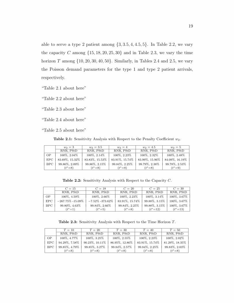
19
able to serve a type 2 patient among {3, 3.5, 4, 4.5, 5}. In Table 2.2, we vary
the capacity C among {15, 18, 20, 25, 30} and in Table 2.3, we vary the time
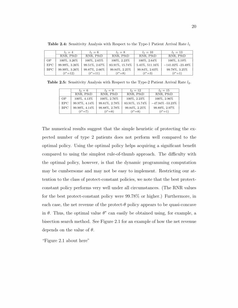
horizon T among {10, 20, 30, 40, 50}. Similarly, in Tables 2.4 and 2.5, we vary
the Poisson demand parameters for the type 1 and type 2 patient arrivals,
respectively.
“Table 2.1 about here”
“Table 2.2 about here”
“Table 2.3 about here”
“Table 2.4 about here”
“Table 2.5 about here”
Table 2.1: Sensitivity Analysis with Respect to the Penalty Coefficient w2.
w2 = 3 w2 = 3.5 w2 = 4 w2 = 4.5 w2 = 5RNR, PStD RNR, PStD RNR, PStD RNR, PStD RNR, PStD
OP 100%, 2.04% 100%, 2.14% 100%, 2.23% 100%, 2.32% 100%, 2.48%
EPC 83.69%, 15.32% 83.83%, 15.53% 83.91%, 15.74% 83.99%, 15.96% 84.09%, 16.19%
BPC 99.86%, 2.09% 99.86%, 2.15% 99.84%, 2.25% 99.79%, 2.38% 99.78%, 2.53%(t∗=8) (t∗=8) (t∗=8) (t∗=8) (t∗=9)
Table 2.2: Sensitivity Analysis with Respect to the Capacity C.
C = 15 C = 18 C = 20 C = 25 C = 30RNR, PStD RNR, PStD RNR, PStD RNR, PStD RNR, PStD
OP 100%, 4.59% 100%, 2.66% 100%, 2.23% 100%, 3.14% 100%, 3.67%
EPC −267.75% -15.09% −7.52% -373.62% 83.91%, 15.74% 99.88%, 3.15% 100%, 3.67%
BPC 99.80%, 4.63% 99.84%, 2.66% 99.84%, 2.25% 99.88%, 3.15% 100%, 3.67%(t∗=1) (t∗=5) (t∗=8) (t∗=12) (t∗=13)
Table 2.3: Sensitivity Analysis with Respect to the Time Horizon T .
T = 10 T = 20 T = 30 T = 40 T = 50RNR, PStD RNR, PStD RNR, PStD RNR, PStD RNR, PStD
OP 100%, 4.77% 100%, 3.25% 100%, 2.55% 100%, 2.23% 100%, 2.02%
EPC 94.29%, 7.58% 90.23%, 10.11% 86.95%, 12.86% 83.91%, 15.74% 81.29%, 18.35%
BPC 99.85%, 4.79% 99.85%, 3.27% 99.84%, 2.57% 99.84%, 2.25% 99.83%, 2.03%(t∗=8) (t∗=8) (t∗=8) (t∗=8) (t∗=8)
20
Table 2.4: Sensitivity Analysis with Respect to the Type-1 Patient Arrival Rate l1
l1 = 4 l1 = 6 l1 = 8 l1 = 10 l1 = 13RNR, PStD RNR, PStD RNR, PStD RNR, PStD RNR, PStD
OP 100%, 3.26% 100%, 2.65% 100%, 2.23% 100%, 2.64% 100%, 3.19%
EPC 99.99%, 3.26% 99.51%, 2.67% 83.91%, 15.74% 5.45%, 511.16% −141.02% -23.49%
BPC 99.99%, 3.26% 99.87%, 2.66% 99.84%, 2.25% 99.84%, 2.63% 99.78%, 3.25%(t∗=12) (t∗=11) (t∗=8) (t∗=3) (t∗=1)
Table 2.5: Sensitivity Analysis with Respect to the Type-2 Patient Arrival Rate l2.
l2 = 6 l2 = 9 l2 = 12 l2 = 15RNR, PStD RNR, PStD RNR, PStD RNR, PStD
OP 100%, 4.13% 100%, 2.76% 100%, 2.23% 100%, 2.96%
EPC 99.97%, 4.14% 99.81%, 2.78% 83.91%, 15.74% −47.94% -53.23%
BPC 99.99%, 4.14% 99.88%, 2.78% 99.84%, 2.25% 99.89%, 2.97%(t∗=7) (t∗=8) (t∗=8) (t∗=1)
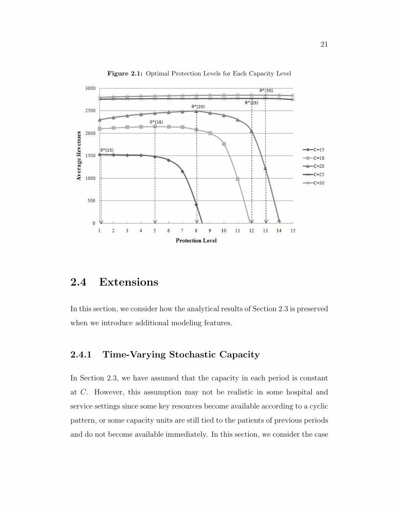
The numerical results suggest that the simple heuristic of protecting the ex-
pected number of type 2 patients does not perform well compared to the
optimal policy. Using the optimal policy helps acquiring a significant benefit
compared to using the simplest rule-of-thumb approach. The difficulty with
the optimal policy, however, is that the dynamic programming computation
may be cumbersome and may not be easy to implement. Restricting our at-
tention to the class of protect-constant policies, we note that the best protect-
constant policy performs very well under all circumstances. (The RNR values
for the best protect-constant policy were 99.78% or higher.) Furthermore, in
each case, the net revenue of the protect-θ policy appears to be quasi-concave
in θ. Thus, the optimal value θ∗ can easily be obtained using, for example, a
bisection search method. See Figure 2.1 for an example of how the net revenue
depends on the value of θ.
“Figure 2.1 about here”
21
Figure 2.1: Optimal Protection Levels for Each Capacity Level
2.4 Extensions
In this section, we consider how the analytical results of Section 2.3 is preserved
when we introduce additional modeling features.
2.4.1 Time-Varying Stochastic Capacity
In Section 2.3, we have assumed that the capacity in each period is constant
at C. However, this assumption may not be realistic in some hospital and
service settings since some key resources become available according to a cyclic
pattern, or some capacity units are still tied to the patients of previous periods
and do not become available immediately. In this section, we consider the case
22
where the capacity available in each period is random.
Let Ct denote a random variable representing the capacity in period t. We
assume that the random variables {Ct|t = 1, . . . , T} are independent from
each other but not necessarily identically distributed. At the beginning of each
period t, the manager observes the realized capacity Ct. Thus, the amount of
capacity to be reserved for type 2 patients should depend on Ct as well as st,
which by x∗t (st, Ct).
For this model, we can show that the properties stated in Theorem 1 con-
tinue to hold. (Proof in Appendix A.2.) Moreover, x∗t (st, Ct) satisfies another
interesting monotonicity property that, for any ε ≥ 0,
0 ≤ x∗t (st, Ct + ε)− x∗t (st, Ct) ≤ ε . (2.5)
This result shows that the protection quantity is an increasing function of the
capacity, but its sensitivity to the capacity availability is limited.
An interesting generalization of this extension is to allow the available capacity
to depend on the number of patients admitted in previous periods. This
enables us to involve patients who may require a resource for multiple periods
in the model. While it is interesting, we are unable to show the properties of
Theorem 1 in this case due to difficulties as the curse of dimensionality, and
leave it for future research. However, the results of this section show that the
properties stated in Theorem 1 are quite robust, and furthermore, a similar
monotonicity property of x∗t exists with respect to the available capacity Ct,
as shown in (2.5).
23
2.4.2 Rejecting Type 1 Patients
In this section, we consider the possibility of rejecting type 1 patients. We now
allow that when a patient of type 1 arrives at the system, the manager may
turn her away to ensure high quality of service for those already admitted to
the hospital.
We modify the model by introducing another decision at the the end of period
t, which determines how many of the new Mt type 1 patients are to be accepted
into the system. Note that, at the end of period t, the number of type 1
patients who have arrived in period t− 1 or earlier and are backlogged equals
(st + xt − C)+. Let at ∈ [0,Mt] denote the number of type 1 patients from
period t that will join the waiting list. In Section 2.3, we had at = Mt, but we
now modify (2.2) to reflect this decision:
ft(st) = max0≤xt≤C
[L(st, xt)
+ α · EMt
{max
0≤at≤Mt
−r1 · (Mt − at) + ft+1((st + xt − C)+ + at)
}].
(2.6)
(Above, the term −r1 · (Mt − at) represents the amount of lost revenue asso-
ciated with accepting at patients only – see the definition of L in (2.1).)
We remark that the value of at is chosen at the end of a period after Mt is
realized, whereas the xt decision is made at the beginning of a period.
Based on the concavity properties of ft, it can be shown that the optimal
accept/reject policy for type 1 patients is a threshold policy, i.e., there exists
24
Rt such that the optimal value of at satisfies
at(zt) =
0 if zt > Rt
Rt − zt if zt ≤ Rt and zt +Mt ≥ Rt
Mt if zt +Mt < Rt,
(2.7)
where zt = (st + xt − C)+ is the number of outstanding type 1 patients from
period t − 1 or earlier. Furthermore, the monotonicity result of Theorem 1
continues to hold in this case. (Proof in Appendix A.3.)
2.4.3 Multiple Elective Patient Classes
Next, we extend the model of Section 2.3 to the case with multiple classes
of type 1 patients. We distinguish these classes with respect to the potential
revenue.
Suppose now that there are n classes of type 1 patients, and we use the su-
perscript to identify each of the n type-1 classes, {1, . . . , n}. We assume that
penalty coefficients satisfy w11 ≥ · · · ≥ wn1 , and also the end-of-horizon ter-
minal values per type 1 patient satisfy v1 ≤ · · · ≤ vn ≤ 0. These orderings
are used to signify that class i patients are more “important” than class j
patients, for i < j. Let w1 = (w11, . . . , w
n1 ) and v = (v1, . . . , vn). Also, let
r1 = (r11, . . . , r
n1 ) denote the per-patient revenue vector.
Let st = (s1t , . . . , s
nt ) denote the vector of backlogged type 1 patients at the
beginning of a period t, and let xt denote the amount of capacity protected
for type 2 arrivals. Thus, C − xt units of capacity will be available to serve
backlogged type 1 patients. Since it is more costly to delay the service of the
patients belonging to a lower-indexed class, a sample path argument can be
used to show that the remaining capacity of C − xt units will be allocated
25
among the type 1 patients in an increasing order of their class indices. Thus,
among the type 1 patients backlogged at the beginning of period t, which is
denoted by st, how many will still be backlogged at the end of the period will
be given by the following function:
ζ(st, C − xt) =
(s1t ∧[s1t − C + xt
]+, s2t ∧[s1t + s2
t − C + xt]+, . . . ,
snt ∧
[n∑i=1
sit − C + xt
]+).
Then, the single-period net-profit function of (2.1) is given as
L(st, xt) = r2 · E min{xt, Dt}+n∑i=1
ri1 · E[M it ]−
n∑i=1
wi1 · zit − w2 · E[Dt − xt]+ ,
where zt = (z1t , . . . , z
nt ) = ζ(st, C − xt), and Mt = (M1
t , . . . ,Mtn) is the vector
comprised of independent random variables representing the new type 1 patient
arrivals. The dynamic programming formulation in (2.2) can be modified as
ft(st) = max0≤xt≤C
[L(st, xt) + α · EMt [ft+1(zt + Mt)]] ,
where fT+1(sT+1) =∑n
i=1 vi · siT+1.
For this model, we can establish results that are analogous to those of Theorem
1. In particular, we can show that the optimal amount of capacity protected
for class 2 patients, x∗t (st) is decreasing in each sit, and the magnitude of this
decrease is limited, i.e., x∗t (st + ε · ei) ≥ x∗t (st) − ε, for any ε > 0, where ei is
the vector consisting of all zeros except the i’th component being 1. (Proof in
Appendix A.4.)
26
2.5 Conclusion
In this chapter, we have developed a dynamic programming model to solve the
resource allocation problem of a health-care facility, and presented the charac-
teristics of the optimal policy and a simple heuristic policy that performs well.
Although our model has been developed in a hospital setting, it is readily ap-
plicable in other service environments with backlogging and lost sales together.
It has been noted earlier that the research on the multiple-demand-inventory
inventory systems with lost sales and backorders is far from being complete,
and our work here has shown that multiple demand classes in service systems
share similar difficulties. The model we propose and the results we obtain dis-
close some understanding of the hospital resource management, but there are
several questions that this research raises. Future research that incorporate
the arbitrary length-of-stay distributions for one or multiple patient types or
a limited waiting time for backlogged patients might prove useful.
27
Chapter 3
An Analysis of Dynamic
Bilateral Price Negotiations
3.1 Introduction
Many transactions between a seller and a buyer follow some form of a negoti-
ation. This is typical in business-to-business settings, e.g., in procurement of
goods and services, as well as in transactions that involve end consumers for
items that are expensive such as cars, furniture, and real-estate. The outcome
of each such negotiation depends on the reservation values of the seller and
buyer, their respective negotiation skill, and their beliefs about these param-
eters for their respective counterparties. This process is known as “bilateral
price negotiation” and studied extensively in the literature (see Nash (1950),
Harsanyi (1956), Myerson (1979), Myerson and Satterthwaite (1983), Myer-
son (1984), and Chatterjee and Samuelson (1983)). Depending on the market
28
conditions, the seller may enjoy increased market power and as such be able
to name her list price in the negotiation, whereas in the other extreme the
buyers may essentially submit take-it-or-leave-it bids to the seller. In most
settings, actual behavior falls somewhere in between, where the seller and
buyer somehow split the difference between the seller’s minimum acceptable
bid (her reservation price, which may be dynamic) and the buyer’s willingness
to pay. However, in today’s business world, “the shifting balance of power has
many stores scrambling for pricing strategies that get beyond the time-worn
cycle of markups and discounts” as stated in a recent NY Times article (Clif-
ford (2012)). Thus, there is a power shift towards the consumers, propelled
by the Internet and apps, which has rendered the buyers more empowered in
haggles, thus demanding much lower prices.
One motivating application for the paper comes from the residential real es-
tate industry, where a developer of a multi-unit project, e.g., a multi-story
condominium development, tries to sell various condos to prospective buy-
ers through a sequence of negotiations over time. While for each buyer their
respective negotiation could be modeled as a one-off interaction, the seller’s
behavior should consider the fact that she will engage into a sequence of such
negotiations over time. The phenomenon of power shift to the advantage of
buyers is also observed in the real estate industry since the explosion of the
real-estate bubble in the financial crisis of 2007. Hence, our main focus is the
changing trading problem and the new pricing strategies of the sellers in the
real-estate setting, even though most of our findings do apply to the general
case. 1
1Numerous articles in the press exemplify the phenomenon that “properties once sold atvery high monetary terms are now being purchased by the bidders who pay the minimumamount to cover back taxes, interest and fees” Sinclair (2009). Many developers of multi-unit residential projects, such as condos, are advertising in the newspapers, magazines and
29
In more detail, we study the revenue maximization problem of a firm that has
C units of capacity that it wishes to sell over a time horizon of length T to
a market of prospective buyers that arrive to the firm according to a Poisson
process with rate Λ, each has a willingness-to-pay that is an independent draw
from a distribution Fb, and who engages in a bilateral negotiation with the
seller for one unit of that good. The salvage value of the seller is private
information, and buyers assume that it is drawn form some distribution Fs,
and it is constant over time. The reservation price of the seller at time t
depends on the salvage value and the state of the sales process, i.e., the time-
to-go and remaining capacity. The bilateral negotiation is modeled as a one-
off negotiation, where the buyer and seller submit bids and where the unit is
warded if the buyer’s bid is higher than the seller’s bid. When the seller has
market power, the transaction price is the seller’s posted price (SPP); when
the buyer has market power, the transaction price is the buyer’s posted price
(BPP); in other cases the transaction price splits the difference between the
two bids according to a fixed ratio that models the relative negotiation power
of the two players. 2
The ultimate focus of this part is to study this problem primarily in the setting
where buyers have market power (BPP), and where the seller and the buyers
do not know the distributions Fb, Fs, respectively, and moreover the unknown
distribution Fb may be changing over time. This setting is motivated by the
real estate application, where there is significant uncertainty about the current
and future market conditions, and where the sales horizon is sufficiently long
so that the market conditions will change over time; the non-stationarity here
on the internet announcing that all bids are welcome.2A detailed definition of each negotiation mechanism can be found in Bhandari and
Secomandi (2009).
30
is not due to seasonality effects that can be readily incorporated in a setting
where the seller would know the evolution of Fb over time, but rather due to
changes in underlying market conditions, e.g., such as interest rates, economic
conditions, etc., that “modulate” the buyer willingness-to-pay distribution.
Despite the importance and prevalence of negotiation problems in practice,
most literature in quantitative dynamic pricing and revenue management has
focused on posted price mechanisms (see Gallego and van Ryzin (1994), Varma
and Vettas (2001)) and auctions (see Vulcano et al. (2002)). Among the
papers that involve revenue management problems in the form of bilateral
negotiations, the work Bhandari and Secomandi (2009) is perhaps closest
to ours regarding the problem under consideration. However, we consider a
setting where the valuation distributions are unknown, and employ an entirely
different methodology than Bhandari and Secomandi, who use a stylized MDP
to investigate the negotiation processes in a dynamic setting. We also mostly
restrict our analysis to a setting where buyers have market power, which is
also the main difference of our work from those of Riley and Zeckhauser (1983)
and Gallien (2006).
The first modeling and methodological contribution of the paper is in formu-
lating the classical bilateral negotiation problem in an uncertain environment,
where buyers and the seller do not have information about Fs, Fb, respectively.
There are three natural ways to specify this type of model uncertainty that
lead to different formulations and different policy recommendations. The first
one is stochastic, wherein the unknown distributions are assumed to be drawn
from a given set of possible distributions according to some known probability
law, and where the firm’s goal is to optimize its expected revenues -potentially
risk-adjusted- over all possible market model realizations. Its main shortcom-
31
ing is that it requires detailed information on the distribution of the model
uncertainty, which itself may not be available. The second formulation adopts
a worst-case perspective using a max-min criterion for both the seller and
buyer, wherein the unknown distributions are assumed to be selected from an
appropriate set of possible distributions by an imaginary adversary (“nature”)
to reduce the seller’s revenue or the buyer’s surplus, and where the seller’s and
buyer’s objective is to select a biding strategy that optimizes their respective
worst-case revenue performance. As a second formulation, both the seller and
the buyer adopt a max-min criterion where they aim to optimize their respec-
tive worst-case revenues. This criterion may yield overly pessimistic results.
To reduce this inherent conservatism, one typically imposes constraints on the
decision set of the adversary, that are either ellipsoids (see Ben-Tal and Ne-
mirovski Ben-Tal and Nemirovski (1998), and El-Ghaoui and Lebret El Ghaoui
and Lebret (1997)), or polyhedra (see Bertsimas and Sim Bertsimas and Sim
(2003), as well as Bertsimas and Thiele Bertsimas and Thiele (2004), Perakis
and Sood Perakis and Sood (2003)). Finally, a third approach that reduces the
conservatism of max-min formulations while maintaining their appealing low
informational requirements is through the use of the competitive ratio or maxi-
mum regret criteria, which measure the performance relative to that of a fully-
informed decision maker. They have been used extensively in the computer
science literature, and have recently been applied in pricing and operations
management problems. Specifically, Ball and Queyranne Ball and Queyranne
(2009) used a competitive ratio criterion for a single-resource capacity allo-
cation problem, while Bergemann and Schlag Bergemann and Schlag (2008),
Eren and Maglaras Eren and Maglaras (2010), and Perakis and Roels Perakis
and Roels (2007) adopted the regret criterion to study the monopolist pric-
ing and the newsvendor problems, respectively. Lan et al. Lan et al. (2006)
32
generalize Ball and Queyranne’s analysis and extend it to cover the regret
criterion as well. Perakis and Roels (2007) applies similar techniques for net-
work revenue management. Eren and Van Ryzin Eren and van Ryzin (2006)
apply these criteria to the problems of product positioning and differentiation.
Specifically, Ball and Queyranne Ball and Queyranne (2009), Bergemann and
Schlag Bergemann and Schlag (2008), Eren and Maglaras Eren and Maglaras
(2010), Perakis and Roels Perakis and Roels (2007), Lan et al. Lan et al. (2006)
and Eren and Van Ryzin Eren and van Ryzin (2006) adopt different versions
of this idea.
Secondly, focusing on a buyer market, we carry the analysis to the dynamic
setting. The key finding is to recognize that in the BPP setting where the seller
is simply making accept or reject decisions of the buyer bids can be reduced
to a single resource capacity control problem in the form analyzed by Lee and
Hersh Lee and Hersh (1998). Specifically, the distribution of buyer bids is
analogous to a continuous distribution of fare classes. This observation allows
us to completely characterize the structure of the optimal policy. We note in
passing that the setting where sellers have market power (SPP) is similarly
analogous to the well-studied dynamic pricing problem studied in Gallego and
van Ryzin Gallego and van Ryzin (1994).
Next, motivated by the goal of studying the dynamic revenue maximization
in settings where the distributional assumptions may be not known and also
change over time, we start with a simpler approximated problem where the
buyer arrival process is replaced by a deterministic and continuous process.
This model can be justified as a limit as the capacity and market potential as
captured by Λ grow large, and the sales horizon and distributional assumptions
stay unchanged. In the limit model the sales process is continuous, where
33
infinitesimal buyers request infinitesimal quantities of the seller’s capacity.
This is often referred to as a “fluid” model. The fluid revenue maximization
problem admits a static solution, as it could be expected from the mapping of
the BPP formulation to the capacity control problem, where the seller accepts
all bids above a given threshold.
Finally, the last part of the chapter focuses on the real-life applications where
the distributions Fs, Fb are unknown and may vary over time. Motivated by our
previous findings regarding the static uncertain problem, we propose a method
that a) uses the deterministic fluid model, b) adopts uniform distributions for
Fs, Fb, c) considers multiple possible parameter scenarios for the evolution of
these distributions, and d) picks a feedback pricing strategy for the seller to
optimize its regret relative to the full information problem. This problem
can be solved in an open-loop manner to get the best possible strategy for
the seller. This, however, can be improved by optimizing over a set of linear
feedback bidding rules for the seller, that are motivated by the optimal seller
strategy under full information. A set of numerical results show that the regret
formulation and the associated uniform distribution assumption lead to good
results, i.e., modest revenue loss for the seller, in a variety of settings.
The main contributions of this chapter are as follows: First, Adopting the
maximum regret criterion we formulate jointly the buyer and seller bidding
problems in the setting where Fs, Fb are unknown to the respective counter-
parties, and show that the optimal strategies are to bid as if the underlying
distributions Fs, Fb were uniform. This formulation and associated result are
novel, and important on their own right as they offer a robust analogue of
the one-to-one bilateral negotiations problem. Parenthetically, the fact that
the uniform distribution appears as the natural assumption under incomplete
34
information is consistent with results derived in the literature. Secondly, we
draw attention to the analogy between the dynamic bilateral negotiation prob-
lems and the classical revenue management problems; which is a first in the
literature. Third, the formulation of the dynamic seller’s problem with uncer-
tain Fs, Fb distributions as a problem that assumes that the distributions are
uniform, as motivated by the result in the one-to-one setting, is novel and the
formulation is itself readily solvable producing a simple and tractable policy
that has a good performance.
The remainder of the chapter. In section 3.2, we consider the one-to-one
negotiation problems: In section 3.2.1, the classical one-to-one negotiation
models are revisited; and in section 3.2.2, we analyze a variant of the classical
problem with an added uncertainty element in terms of the valuation distri-
bution functions. In section 3.3, the analysis is carried to a dynamic setting.
Section 3.3.1 sheds light on the analogy of the negotiation problems with the
revenue management problems. Section 3.3.2 presents the dynamic pricing
model that extends the results of the static negotiation problem to a dynamic
setting using a fluid model approach. Next, in section 3.4, the results of section
3.2.2 are extended to the dynamic setting again under a regret criterion. In
particular, we propose a scenario-based robust optimization approach which is
both tractable and takes into account the unfolding uncertainty in the system
as time progresses. Numerical illustrations and extensions are presented in
Section 3.5. Finally, section 3.6 concludes our findings and presents avenues
for further research.
35
3.2 1-to-1 Bilateral Negotiation Problem
In Section 3.2.1, we present the classical one-to-one negotiation problem that
forms the building blocks for the dynamic negotiation problem studied in Sec-
tion 3.3. Then in Section 3.2.2, we analyze a variant of the classical one-to-one
bilateral negotiation problem with an added uncertainty element in terms of
the valuation distribution functions which, to best of our knowledge, has not
been attempted before.
3.2.1 Classical 1-to-1 Bilateral Negotiation Problem
Although the literature of two-person bargaining games goes back to Nash
(1950) and Harsanyi (1956), the first pieces of work to pioneer the analysis of
the dynamics of an environment where the buyers have the major market power
are those of Myerson (et al.) (Myerson (1979), Myerson and Satterthwaite
(1983), Myerson (1984)) and of Chatterjee and Samuelson (1983). However,
even in the alluded studies, the negotiation problem is only analyzed within
a static context where the game is between a single seller and a single buyer.
In this paper, we will extend the previous line of research into a dynamic
setting. But first, let us revisit the classical one-to-one negotiation problem of
the literature.
The one-to-one bilateral negotiation problem involves the trading interactions
between two individuals where one of the individuals (the seller) owns an ob-
ject that the other (the buyer) wants to buy. Both players are risk neutral.
From the seller’s perspective the valuation of the buyer for this unit is ran-
dom variable vb, distributed according to probability density and distribution
36
functions fb and Fb with support [¯vb, vb]. A symmetric argument holds for
the buyer, where he assumes that the seller’s valuation for the unit, vs, is
distributed according to cumulative distribution function Fs (with p.d.f. fs)
on the range [¯vs, vs]. Fs and Fb are both strictly increasing and differentiable
on their supports, and are common knowledge in the sense of Aumann (1976)-
that is, each side knows these distributions, knows that they are known by the
other side, knows that the latter knowledge is known, and so on and so forth.
The rules of the bargaining game is as follows: At the beginning of the sales
interval the seller sets a reservation price s(vs), then the buyer submits a bid
b(vb), and a successful trade is concluded if b(vb) exceeds s(vs). The resulting
sales price is kb(vb) + (1 - k)s(vs), where k ∈ [0, 1] is a parameter that deter-
mines the bargaining power of the buyers. Specifically, if k = 0, the problem
reduces to a “seller posted price” (SPP) setting where the entire power to de-
termine the final price lies with the seller: In this case, the trade is concluded
at the price s(vs) as long as s(vs) ≤ b(vb). At the other extreme, when k = 1,
the problem simply becomes a “buyer posted price” (BPP) formulation where
the sales price is equivalent to the buyer’s bid b(vb), again provided that s(vs)
≤ b(vb) holds.
Chatterjee and Samuelson (1983) characterize the class of equilibria for the
above problem in which player bidding strategies are “well-behaved”. In par-
ticular, they make the following assumption regarding the buyer and seller
bidding functions s(.) and b(.), which is also relevant for our further analyses:
Assumption 1. In the equilibrium, both b(.) and s(.) are bounded above and
below and are strictly increasing and differentiable except possibly at the bound-
ary points.
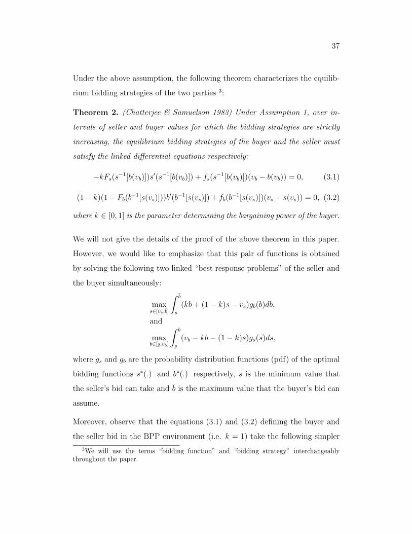
37
Under the above assumption, the following theorem characterizes the equilib-
rium bidding strategies of the two parties 3:
Theorem 2. (Chatterjee & Samuelson 1983) Under Assumption 1, over in-
tervals of seller and buyer values for which the bidding strategies are strictly
increasing, the equilibrium bidding strategies of the buyer and the seller must
satisfy the linked differential equations respectively:
−kFs(s−1[b(vb)])s′(s−1[b(vb)]) + fs(s
−1[b(vb)])(vb − b(vb)) = 0, (3.1)
(1− k)(1− Fb(b−1[s(vs)]))b′(b−1[s(vs)]) + fb(b
−1[s(vs)])(vs − s(vs)) = 0, (3.2)
where k ∈ [0, 1] is the parameter determining the bargaining power of the buyer.
We will not give the details of the proof of the above theorem in this paper.
However, we would like to emphasize that this pair of functions is obtained
by solving the following two linked “best response problems” of the seller and
the buyer simultaneously:
maxs∈[vs,b]
∫ b
s
(kb+ (1− k)s− vs)gb(b)db,
and
maxb∈[
¯s,vb]
∫ b
¯s
(vb − kb− (1− k)s)gs(s)ds,
where gs and gb are the probability distribution functions (pdf) of the optimal
bidding functions s∗(.) and b∗(.) respectively,¯s is the minimum value that
the seller’s bid can take and b is the maximum value that the buyer’s bid can
assume.
Moreover, observe that the equations (3.1) and (3.2) defining the buyer and
the seller bid in the BPP environment (i.e. k = 1) take the following simpler
3We will use the terms “bidding function” and “bidding strategy” interchangeablythroughout the paper.
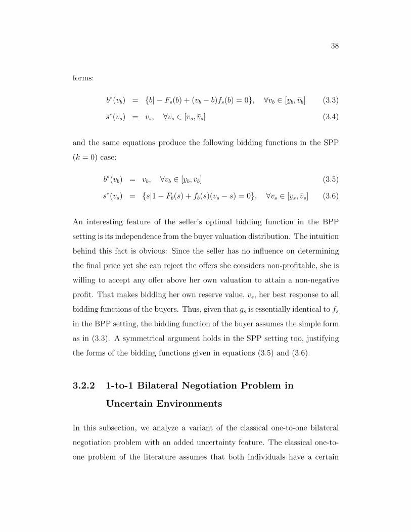
38
forms:
b∗(vb) = {b| − Fs(b) + (vb − b)fs(b) = 0}, ∀vb ∈ [¯vb, vb] (3.3)
s∗(vs) = vs, ∀vs ∈ [¯vs, vs] (3.4)
and the same equations produce the following bidding functions in the SPP
(k = 0) case:
b∗(vb) = vb, ∀vb ∈ [¯vb, vb] (3.5)
s∗(vs) = {s|1− Fb(s) + fb(s)(vs − s) = 0}, ∀vs ∈ [¯vs, vs] (3.6)
An interesting feature of the seller’s optimal bidding function in the BPP
setting is its independence from the buyer valuation distribution. The intuition
behind this fact is obvious: Since the seller has no influence on determining
the final price yet she can reject the offers she considers non-profitable, she is
willing to accept any offer above her own valuation to attain a non-negative
profit. That makes bidding her own reserve value, vs, her best response to all
bidding functions of the buyers. Thus, given that gs is essentially identical to fs
in the BPP setting, the bidding function of the buyer assumes the simple form
as in (3.3). A symmetrical argument holds in the SPP setting too, justifying
the forms of the bidding functions given in equations (3.5) and (3.6).
3.2.2 1-to-1 Bilateral Negotiation Problem in
Uncertain Environments
In this subsection, we analyze a variant of the classical one-to-one bilateral
negotiation problem with an added uncertainty feature. The classical one-to-
one problem of the literature assumes that both individuals have a certain
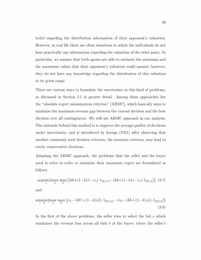
39
belief regarding the distribution information of their opponent’s valuation.
However, in real life there are often situations in which the individuals do not
have practically any information regarding the valuation of the other party. In
particular, we assume that both agents are able to estimate the minimum and
the maximum values that their opponent’s valuation could assume; however,
they do not have any knowledge regarding the distribution of this valuation
in its given range.
There are various ways to formulate the uncertainty in this kind of problems,
as discussed in Section 3.1 in greater detail. Among these approaches lies
the “absolute regret minimization criterion” (ARMC), which basically aims to
minimize the maximum revenue gap between the current decision and the best
decision over all contingencies. We will use ARMC approach in our analysis.
The rationale behind this method is to improve the average quality of decisions
under uncertainty; and is introduced by Savage (1951) after observing that
another commonly used decision criterion, the maximin criterion, may lead to
overly conservative decisions.
Adopting the ARMC approach, the problems that the seller and the buyer
need to solve in order to minimize their maximum regret are formulated as
follows:
argmins{max
bmaxs′
[(kb+(1−k)s′−vs)·1{b≥s′}−(kb+(1−k)s−vs)·1{b≥s}]} (3.7)
and
argminb{max
smaxb′
[(vb−(kb′+(1−k)s)) ·1{b′≥s}−(vb−(kb+(1−k)s)) ·1{b≥s}]}
(3.8)
In the first of the above problems, the seller tries to select the bid s which
minimizes the revenue loss across all bids b of the buyer; where the seller’s
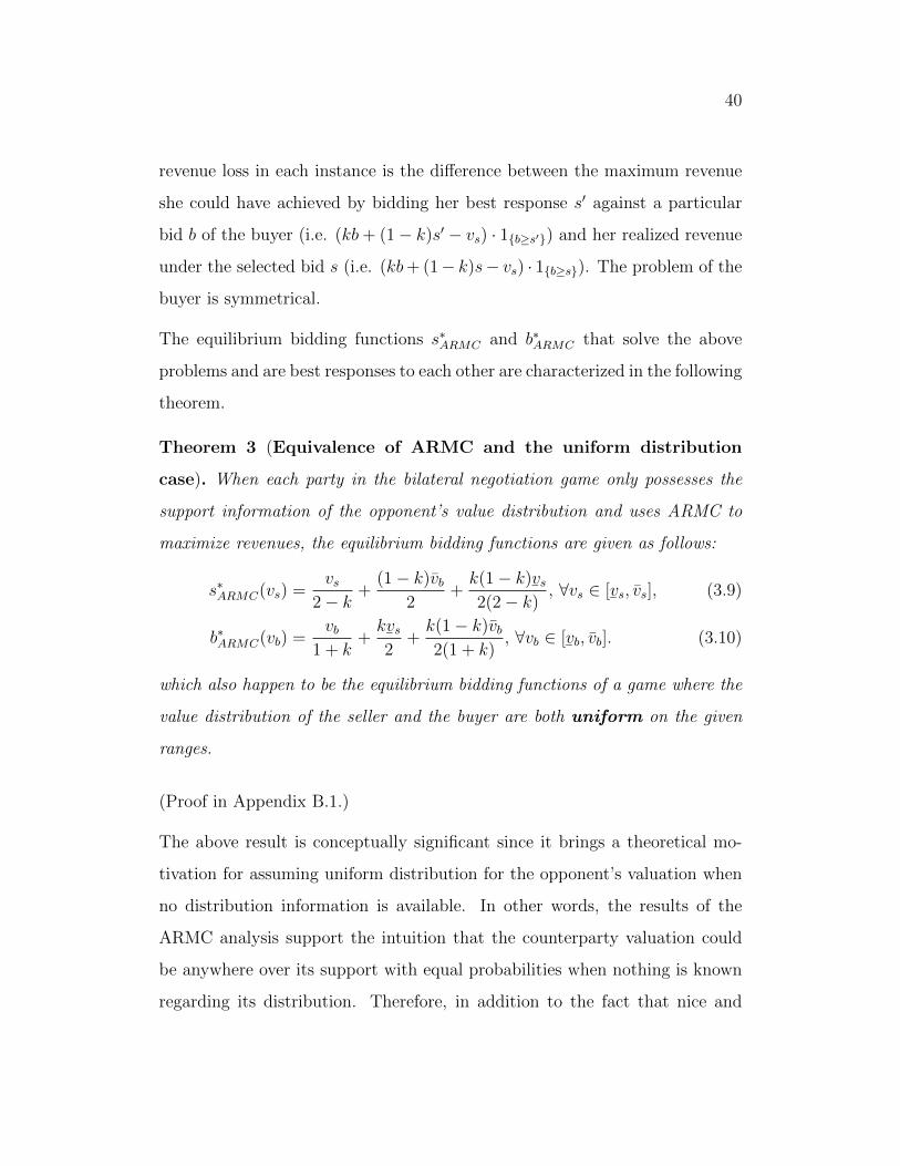
40
revenue loss in each instance is the difference between the maximum revenue
she could have achieved by bidding her best response s′ against a particular
bid b of the buyer (i.e. (kb+ (1− k)s′ − vs) · 1{b≥s′}) and her realized revenue
under the selected bid s (i.e. (kb+ (1− k)s− vs) · 1{b≥s}). The problem of the
buyer is symmetrical.
The equilibrium bidding functions s∗ARMC and b∗ARMC that solve the above
problems and are best responses to each other are characterized in the following
theorem.
Theorem 3 (Equivalence of ARMC and the uniform distribution
case). When each party in the bilateral negotiation game only possesses the
support information of the opponent’s value distribution and uses ARMC to
maximize revenues, the equilibrium bidding functions are given as follows:
s∗ARMC(vs) =vs
2− k+
(1− k)vb2
+k(1− k)
¯vs
2(2− k), ∀vs ∈ [
¯vs, vs], (3.9)
b∗ARMC(vb) =vb
1 + k+k¯vs2
+k(1− k)vb2(1 + k)
, ∀vb ∈ [¯vb, vb]. (3.10)
which also happen to be the equilibrium bidding functions of a game where the
value distribution of the seller and the buyer are both uniform on the given
ranges.
(Proof in Appendix B.1.)
The above result is conceptually significant since it brings a theoretical mo-
tivation for assuming uniform distribution for the opponent’s valuation when
no distribution information is available. In other words, the results of the
ARMC analysis support the intuition that the counterparty valuation could
be anywhere over its support with equal probabilities when nothing is known
regarding its distribution. Therefore, in addition to the fact that nice and
41
neat closed-form solutions can be obtained by assuming that the opponent’s
value is distributed uniformly in its given range, we have also established a
theoretical motivation to use the uniform distribution assumption in this type
of games.
Remark 1. By the above analysis, we have extended the literature on the one-
to-one negotiation problem between a single seller and a single buyer where
neither the seller nor the buyer know each other’s distribution function, but
they both know the range of the opponent valuations. It is also possible to
analyze a third case where one of the parties is informed about the other’s value
distribution function, while the other only knows the range of his opponent’s
valuation. The solution for this case can be found in Appendix B.2.
3.3 Dynamic Bilateral Negotiation Games
In this section, we turn our attention to the main objective of the chapter
and analyze the dynamic problem of a revenue maximizing monopolist who
sells a number of homogeneous units over a finite sales horizon to a market
of prospective buyers that arrive according to a (possibly non-homogeneous)
Poisson process, where each transaction is a one-off bilateral negotiation game.
3.3.1 The Analogy Between the Revenue Management
and Bilateral Negotiation Problems
Consider the general revenue maximization problem of a monopolist firm: If
the firm operates in a market with imperfect competition, it has the power to
determine the sales price. In this setting, the firm’s problem is to choose a dy-
42
namic pricing strategy which is changing according to the remaining inventory
and the expected customer arrivals, with the objective of maximizing expected
revenues. If, however, the prices are exogenously determined by competition
or through a higher order optimization problem defining the market conditions
(as in our case, by the equilibrium in the negotiation game between the buyers
and the seller), the firm chooses a dynamic capacity allocation rule that con-
trols when to accept new requests for its products. These two problems, which
we will refer to as the “dynamic pricing” and “capacity allocation” problems
respectively in the sequel, are the two famous problems of the revenue man-
agement and pricing literature and have elicited much attention from various
groups of researchers. For instance, the stochastic dynamic pricing game has
been extensively analyzed by Gallego and van Ryzin (1994) (which will be re-
ferred to as GVR for the rest of the paper) and the capacity rationing problem
of a single resource has also been considered by many researchers, involving
Lee and Hersh (1998) and Brumelle and McGill (1993) among many others.
In our case, we consider a sequence of independent bilateral negotiation games
played between the seller and each one of the buyers arriving over a finite
sales horizon. The seller would like to sell C units of a homogeneous good
over a sales horizon T where each arriving buyer interacts with the seller for
a single unit of the good according to a one-off bilateral negotiation game.
Potential customers arrive according to a non-homogeneous Poisson process
with instantaneous rate Λt. Each customer has a valuation vb for the product
which is an independent draw from a cumulative distribution function Fb. The
willingness-to-pay (WtP) value of a buyer with valuation vb is therefore b∗(vb),
which is characterized by the equation (3.1) regardless of his arrival time t.
Next, the seller quotes a minimum reserve price st(vs), and the unit is sold if
43
bt(vb) = b∗(vb) > st(vs); otherwise the customer leaves without purchasing a
unit.
The key observation in the dynamic setting is that the buyers in the system
are “naive”: they ignore the competition with other buyers in the market, and
bid according to the equilibrium bidding function b∗(·) characterized by the
equation (3.1). However, the seller will engage into a sequence of such negoti-
ations over time, therefore submits her bid with the objective of maximizing
her overall revenues. Thus, the seller’s bid is no longer determined by the
equation (3.2).
First, consider an SPP setting: We know that in this environment the buyer
equilibrium bidding function takes the form b∗SPP (vb) = vb. Hence, given the
arrival rate Λt, it is possible to define the expected “sales rate” function at
the instant t by N(t) = N(st) = ΛtFb(st) which is a “regular function” in the
sense that regular functions are defined in GVR paper provided that st lies in
a compact set P (Namely, N(t) is strictly decreasing in st, limst→∞N(st) = 0,
and the revenue rate stΛtFb(st) is bounded for all st ∈ P and has a finite
maximizer).
We adopt a discrete-time formulation where time has been discretized to small
intervals of length δt, indexed by t = 1, . . . , T such that P(a buyer arrives at
[t− δt, t]) = Λtδt+ o(δt) where o(x) implies that o(x)/x→ 0 as x→ 0. Thus,
the random sales amount at instant t, which we will denote by ξ(t;N), is
Bernoulli with probability P(ξ(t;N) = 1) = N(st)δt and P(ξ(t;N) = 0) =
1−N(st)δt for small δt.
Thus, the seller’s revenue maximization problem in an SPP setting could be
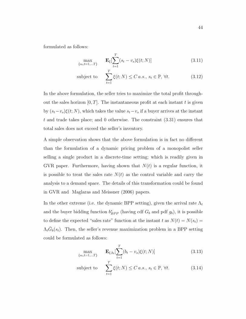
44
formulated as follows:
max{st,t=1,...T}
Eξ[T∑t=1
(st − vs)ξ(t;N)] (3.11)
subject toT∑t=1
ξ(t;N) ≤ C a.s., st ∈ P, ∀t. (3.12)
In the above formulation, the seller tries to maximize the total profit through-
out the sales horizon [0, T ]. The instantaneous profit at each instant t is given
by (st−vs)ξ(t;N), which takes the value st−vs if a buyer arrives at the instant
t and trade takes place; and 0 otherwise. The constraint (3.31) ensures that
total sales does not exceed the seller’s inventory.
A simple observation shows that the above formulation is in fact no different
than the formulation of a dynamic pricing problem of a monopolist seller
selling a single product in a discrete-time setting; which is readily given in
GVR paper. Furthermore, having shown that N(t) is a regular function, it
is possible to treat the sales rate N(t) as the control variable and carry the
analysis to a demand space. The details of this transformation could be found
in GVR and Maglaras and Meissner (2006) papers.
In the other extreme (i.e. the dynamic BPP setting), given the arrival rate Λt
and the buyer bidding function b∗BPP (having cdf Gb and pdf gb), it is possible
to define the expected “sales rate” function at the instant t as N(t) = N(st) =
ΛtGb(st). Then, the seller’s revenue maximization problem in a BPP setting
could be formulated as follows:
max{st,t=1,...T}
Eξ,bt [T∑t=1
(bt − vs)ξ(t;N)] (3.13)
subject toT∑t=1
ξ(t;N) ≤ C a.s., st ∈ P, ∀t. (3.14)
45
where bt := b∗BPP (vt), and the valuation vt of the buyer arriving at instant t is
randomly drawn from the valuation range of the buyers. However, note that
the price st now has no direct effect on the revenue at the instant t, except
for determining the lower bound of the buyer bids to be admitted. That is, it
effectively works as a control that leads to “opening” product classes (buyer
bids) that exceed the price level st and “closing” classes that bring lower
revenue than st. Hence, we will proceed by the following approximation to
show the connection of the above problem with the capacity allocation problem
of the literature: Assume that we can approximate all buyer bids by n finite
values; i.e. define b∗ ≥ b1 ≥ b2 ≥ . . . ≥ bn ≥¯b∗ as n finite “fare classes”,
where the arrival rate of bid bi is approximated by Λt(Gb(bi) − Gb(bi−1)),
∀i ∈ {2, . . . , n} and the arrival rate of b1 is approximated by ΛtGb(b1) at
each instant t. Then, the problem above pours into the following capacity
allocation problem of a firm which has discretion as to which product requests
to accept at any given time:
max{u(t),t=1,...T}
Eξ[T∑t=1
(b′ − vs)ξ(t;uΛ)] (3.15)
subject toT∑t=1
e′ξ(t;uΛ) ≤ C a.s., ui(t) ∈ {0, 1}, ∀t.
where ui(t)’s are the controls that take value 1 when a bid of value bi is
accepted at time t and zero otherwise, b′ = {b1, b2, . . . , bn}, e′ the n-dimensional
unit vector, and ξ(t;uΛ) denotes the associated sales vector. It is then easily
observed that the formulation (3.15) is the discretized version of the capacity
control problem of Lee and Hersh (1998).
Thus, if the buyer bids could be approximated by a finite class of fares, the
BPP formulation is equivalent to the capacity allocation problem of a seller
46
selling a single resource to multiple demand classes in a perfect competition
setting. For details, we refer the reader to Lee and Hersh (1998) and Maglaras
and Meissner (2006).
The two above equivalences stem from the fact that while the buyers are naive,
the seller will engage into a sequence of negotiation games over the sales hori-
zon, and therefore submits her bid with the objective of maximizing her overall
revenues. Hence, in the first game she will pursue a dynamic pricing strategy
to maximize the revenues to be extracted from the stochastically arriving buy-
ers; whereas in the second game, she will determine the minimum bid to be
accepted at each time instant to control the amount of capacity to be sold.
Therefore, in broad terms, the SPP game reduces to the dynamic pricing and
the BPP game to the capacity allocation problems of the literature. We state
this result as a proposition.
Proposition 1. If the buyers in the market are naive, given that the equilib-
rium bidding functions of the one-to-one game are known, the dynamic SPP
game becomes equivalent to the dynamic pricing problem and the dynamic
BPP game to the capacity allocation problem of the revenue management
literature.
Although theoretically simple to characterize, the above problems are often
very hard to compute numerically. For instance, in the case of the dynamic
pricing problem, the authors have adopted a fluid formulation in the GVR
paper and developed asymptotically optimal policies. Also, in negotiation
problems, there is a continuous stream of buyer bids often with their range and
frequency varying in time; therefore it is practically impossible to approximate
the buyer bids as finite number of fare classes as we did above. Even if this
approximation is valid, the issue of “curse of dimensionality” prevails. Thus,
47
the size of the problem renders the computation of the optimal bids st, ∀t,
almost impossible, which leads us to develop a fluid-formulation equivalent
of the dynamic negotiation problems and focus on the analysis in this fluid
setting.
Finally, we would like to note that the relationship between the dynamic pric-
ing and capacity allocation problems is extensively studied in Maglaras and
Meissner (2006), in which work the authors illustrate how the two problems
can be reduced to a common formulation by tracking the aggregate capacity
consumption rates. We will pursue a similar objective and help to establish
the connection between the two extreme negotiation problems by showing that
the structural results of GVR also hold in the BPP setting.
3.3.2 Fluid Formulation of the Dynamic Game
Since analyzing the stochastic dynamic pricing problem of the seller is difficult,
we will proceed with a fluid formulation in the hope to obtain possible insights
towards the stochastic problem. As commonly known, fluid formulation is a
good approximation of the real stochastic problem when number of interactions
per unit time is sufficiently large.
To this end, consider the following fluid formulation of the general dynamic
negotiations game: Infinitesimal buyers arrive with a (deterministic) rate Λt
at t, t ∈ [0, T ]. The buyer and the seller valuation functions have the same
characteristics as defined in the one-to-one setting. Both parties know Λt
and the distribution function of their opponent. In this setting, the revenue
48
maximization problem of the seller takes the following form:
maxst,∀t
[
∫ T
0
rt(vs, st)dt] (3.16)
subject to
∫ T
0
Λt[
∫ b
st
gb(b) db] dt ≤ C (3.17)
where rt(vs, st) is the instantaneous net revenue function of the seller at time
t when her valuation is vs and her reservation price st; which is given by:
rt(vs, st) =
∫ b
st
Λt(kb+ (1− k)s(vs)− vs) gb(b) db. (3.18)
and gb is the pdf of the buyer bidding function b characterized in (3.1) and s(·)
is given by (3.2). (For the rest of the analysis, the terms b∗(.) and gb will refer
to these functions as well as Gb, which will denote the cdf of b∗, unless stated
otherwise.) Observe that we do not need a subscript t in the bidding function
b∗(·) of the buyers, since the distribution of b∗ is the same at all instances t in
the equation (3.18) given that the buyers are naive.
It is usually difficult to find the solution to the above problem if it is modeled as
a stochastic control problem in the price space. Therefore, following a similar
approach as in GVR, we will analyze the problem by focusing on the optimal
sales rate, rather than the optimal pricing policy. Note that the value of each
quantity will follow after the other one is settled.
If the seller sets st as the lowest price to be accepted at t, the fraction of buyers
that are accepted at that instant is given by αt(st) =∫ bstgb(b) db = Gb(st),
inducing an inverse function:
st(αt) = G−1b (1− αt).
The function st(αt) is well-defined for all αt ∈ [0, 1] as a result of Assumption
1.
49
Then, the instantaneous net revenue function of the seller at time t in terms
of the fraction of accepted buyers becomes:
rt,a(vs, αt) =
∫ b
G−1b (1−αt)
Λt (kb+ (1− k)(G−1b (1− αt))− vs) gb(b) db.
Moreover, the seller’s revenue maximization problem (3.16)-(3.17) in the price
space is equivalent to the following formulation in the demand space:
maxαt,∀t
[
∫ T
0
rt,a(vs, αt)dt] (3.19)
subject to
∫ T
0
Λtαt dt ≤ C. (3.20)
Provided that rt,a(vs, α) is concave in α, the formulation (3.19)-(3.20) pours
into the maximization problem of a concave function over a convex set, and
its solution is characterized as in the following Theorem.
Theorem 4. If rt,a(vs, α) is concave in α, the equilibrium bidding strategy
st(.), t ∈ [0, T ], of the seller in the dynamic negotiation problem takes the
form:
st(vs) = max{G−1b (1− C∫ T
t=0Λt dt
), s∗(vs)},∀t ∈ [0, T ], (3.21)
where s∗(vs) is the equilibrium bidding strategy of the seller characterized in
(3.2); the equilibrium bidding strategy bt(.), t ∈ [0, T ], of each infinitesimal
buyer arriving at time t is characterized by the equation (3.1), and Gb is its
cdf.
Proof. As we have already noted, the buyers are naive: i.e. they neither have
the knowledge of the sales rate nor the remaining inventories of the seller.
Therefore, they will regard the situation simply as a one-to-one negotiation
game and employ the static equilibrium bidding function b∗(.) regardless of
their time of arrival.
50
To see how the seller behaves, note that the problem (3.19)-(3.20) is maximized
at the maximizer of rt,a(., vs), which is α∗ := Gb(s∗(vs)), as long as it is feasible
to admit this fraction at each instant t (i.e. if α∗∫ T
0Λt dt ≤ C). This case is
equivalent to applying the bid st(vs) = s∗(vs), ∀t.
If, on the other hand, α∗∫ T
0Λt dt > C, then by the concavity of rt,a(., vs), it
is optimal to admit the constant fraction α0 := C∫ Tt=0 Λtdt
at each t. This second
case corresponds to bidding st(vs) = G−1b (1− C∫ T
t=0 Λt dt), ∀t ∈ [0, T ].
Finally, when α∗ > C∫ Tt=0 Λtdt
, the inequality G−1b (1 − C∫ T
t=0 Λt dt) ≥ s∗(vs) holds;
and the reverse would be true in the opposite case. So the seller will set her
reservation price as st(vs) = max{s∗(vs), G−1b (1 − C∫ T
t=0 Λt dt)}, which ends the
proof of the theorem.
The above theorem is in the same spirit as the Proposition 2 of GVR paper
and forms the first major result of this section.
Regarding concavity of the instantaneous revenue function of the seller, for
instance:
g′b(b) ≥ 0,∀b ∈ [¯b, b] (3.22)
is a sufficient condition to ensure that rt,a(vs, α) is concave in α for all vs ∈
[¯vs, vs]. This condition simply ensures that the second derivative of the function
rt,a(vs, ·) is negative at all α. Observe that both functions Fs, Fb being uniform
is one case where Condition (3.22) is satisfied.
3.3.3 The Informed Buyers in BPP Setting
Until this far, we have assumed the buyers in the market are “naive buyers”
who do not have the knowledge of (or, simply ignore) the seller’s inventory
51
level and the competition in the market. However, in many real life situations,
this may not be the case, and the buyers could observe the inventory level of
the seller and the number of other buyers in the market. In this subsection,
we will briefly analyze the case where the buyers have the knowledge of the
current inventory level xt of the seller and the information regarding the future
market size; and base their decisions on this knowledge.
We will restrict our attention to the BPP setting for this subsection, to see
the possibility whether the competition in the market can nullify the buyers’
advantage of being in a buyer’s market.
To this end, consider a multi-period setting with discrete sales periods indexed
forward as t ∈ {1, 2, . . . , T}. We will employ backward induction to analyze
and solve the problem.
At t = T , when the seller and all the buyers know xT (the number of units in
seller’s hand), Fb, Fs and ΛT , there are two possible cases:
(i) ΛT < xT : In this case, the competition among buyers is not of significance,
since there is ample capacity to serve everyone in the market. So the buyers
will again bid as if they participate in a one-to-one game, i.e. according to
b∗(·) given by (3.3), and the seller will bid her best response against b∗, which
is s∗(vs) = vs.
(ii) ΛT > xT : In this case there is not sufficient capacity to serve the entire
market. Hence, the seller’s revenue maximization problem takes the form:
maxαT
ΛT
∫ bT
G−1bT
(1−αT )
(b− vs) gbT (b) db
subject to ΛTαT ≤ xT (3.23)
where bT is the bidding function of the buyers at t = T , GbT (.) its cdf, and
52
gbT (.) is the pdf. The above problem is clearly maximized at the seller bid
sT (vs) = max{vs, G−1bT
(1 − xTΛT
)}; i.e. the seller is willing to accept all bids
above the maximum of her own valuation and market clearing price.
On the other hand, the revenue maximization problem of each buyer now
becomes:
maxb
∫ b
¯sT
(vb − b)gsT (s)ds (3.24)
where gsT is the pdf of the bidding function sT (·) of the seller.
When these two problems are solved simultaneously, the equilibrium bidding
functions at t = T are found to take the following forms:
Theorem 5. At t = T , when ΛT > xT , the equilibrium bidding functions of
the buyer and the seller take the forms:
sT (vs) = max{(F−1b (1− xT
ΛT
), vs}, (3.25)
and
bT (vb) =
vb, if vb < F−1
b (1− xTΛT
)
F−1b (1− xT
ΛT), if b∗(vb) ≤ F−1
b (1− xTΛT
) ≤ vb
b∗(vb), if F−1b (1− xT
ΛT) < b∗(vb)
where b∗(·) is the equilibrium bidding function of the one-to-one game (i.e.
b∗BPP (·) given by (3.3)).
The proof of the above Theorem simply follows by showing that the pair of
bidding functions sT (·) ad bT (·) satisfy the equations (3.23) and (3.24); and
are best responses to each other. However, we note that in this game the
equilibrium bidding functions no longer comply to the conditions stated in
Assumption 1.
53
Remark 2. When competition among buyers comes into play, the game in
the last period becomes similar to one where all winning buyers pay the first
losing bid (=last winning bid), i.e. a Secondary Price Auctioning Mech-
anism (except for buyers with very high valuations, for whom bidding b∗(vb)(>
first losing bid) is a better option in order to minimize the risk of “no trade”
in the contingency of high valuations of the seller). Note that this result is also
consistent with the findings of Vulcano et al. (2002).
Similarly, for t = 1, 2, . . . , T − 1, the problem can be solved by backwards
induction provided that the seller’s revenue function for t+ 1, . . . , T is known.
However, characterizing the closed form solutions of the bidding functions
grow to be gradually more complicated as we move to earlier time periods.
For instance, consider t = T − 1. Again, if ΛT−1 + ΛT < xT−1, all buyers
act as if in a one-to-one negotiation game against the seller. However, if
xT−1 < ΛT−1 +ΛT , the buyers and the seller should solve simultaneous revenue
maximization problems as follows: Let VT (xT ) denote the seller’s maximum
revenue function when she has xT units of inventory left at t = T . This
function should be easy to characterize since we already know how the agents
will act at t = T for each level of inventory xT given ΛT . Hence, the seller’s
revenue maximization problem at t = T − 1 takes the following form:
maxαT−1
ΛT−1
∫ bT−1
G−1bT−1
(1−αT−1)
(b− vs) gbT−1(b) db
+VT (xT−1 − ΛT−1αT−1)
subject to ΛT−1αT−1 ≤ xT−1
where bT−1(.) is the equilibrium bidding function of the buyers at t = T − 1
and GbT−1its cdf, where the function bT−1(.) is characterized by the following
54
revenue maximization problem of buyers:
maxb
∫ b
¯sT−1
(vb − b)gsT−1(s)ds
where sT−1(.) is the equilibrium bidding function of the seller at t = T − 1.
As before, sT−1 and bT−1 should be best responses to each other.
Note that the above results hold when the buyers can only observe the current
inventory level and know the future market size information. If, on the other
hand, they can also observe the past sales data, then they can infer further
information regarding the valuation of the seller aside from its distribution
information; in which case the above analysis fails to hold any longer.
3.3.4 Dynamic Negotiation Games under Uncertainty
In this part, we study a variant of dynamic negotiation problems where the
primitives of the buyer valuation distribution are unknown. This type of multi-
stage stochastic optimization problems has elicited much interest from various
research communities and there are several established methodologies to ex-
pound them involving dynamic programming, stochastic programming and
robust optimization. However, the problem usually remains hard to solve
analytically. Therefore, in practice, one would typically solve the recursions
numerically or resort to some approximations such as approximate dynamic
programming or simulation. In a similar manner, we will introduce a class of
policies that is motivated by the structure identified in the deterministic ver-
sion of the problem as well as the solution of the stochastic one-to-one problem
and confirm that these policies achieve “good” performance in the dynamic
stochastic problem.
55
The problem setting is as follows: At each instant t, t ∈ [0, T ], independent
dynamic negotiation games take place between the seller and the entire popu-
lation of infinitesimal buyers whose valuation distribution function is revealed
only at the instant t. The players know each other’s distribution range for
all t ∈ [0, T ] (and suppose that, for convenience, this range does not change
across time). In this situation, the ARMC approach is again a viable choice for
all parties. However, at this point we need to make the following assumption
to ignore the “learning effect” for the seller (otherwise, the seller’s problem
becomes trivial as she employs the optimal pricing policy as soon as she finds
out the value distribution function of buyers either by pure observation, or by
inferring from the instantaneous sales amount).
Assumption 2. The seller can neither observe the buyer value distribution
function, Fb, nor the sales amount until the end of the sales horizon.
Although the above assumption might seem unrealistic, it is in fact equivalent
to assuming that the buyers’ valuation distribution is continuously changing
over time. Hence, observing the past sales will not help the seller in predicting
the future sales. Moreover, with no information regarding the future based on
current observations, the seller employs a stationary bidding policy starting at
the instant t, i.e. st = s, ∀t.
With these observations, we are ready to state and prove the following The-
orem, which emphasizes the analogy of the dynamic stochastic problem with
the stochastic one-to-one problem.
Theorem 6. The dynamic stochastic problem with unknown valuation func-
tions but known ranges reduces to the dynamic deterministic problem of section
3.3.2, with Fs and Fb being uniform distribution functions on their given ranges
56
at each t.
(Proof in Appendix B.3.)
3.3.5 A Comparison of Seller Revenues in the
Dynamic SPP vs. BPP Settings
By the analysis in Section 3.3.2, we know that the seller’s optimal bidding
strategy is given by:
st(vs) = max{vs, G−1b (1− C∫ T
t=0Λt dt
)}
in the BPP market; and by:
st(vs) = max{s∗SPP (vs), F−1b (1− C∫ T
t=0Λt dt
)}
in the SPP market. This result makes the analogy between the two problems
more explicit. However, since BPP is a mechanism that favors the buyers; the
two optimal strategies, despite having essentially the same static structure,
may produce very different revenues in SPP and BPP environments. This re-
sult will be more explicit in the numerical examples section. Still, in this part,
we would like to briefly analyze the relationship between the seller revenues in
the two above settings under the assumption of uncertainty; i.e. in the case
where all distributions are assumed to be uniform in their respective ranges.
In this case, letting α0 := 1− C∫ Tt=0 Λt dt
, the seller’s bidding function becomes:
st(vs) = max{vs, ¯vs2
+α0(vb −
¯vb) +
¯vb
2}
in the BPP market, and:
st(vs) = max{vs + vb2
, α0(vb −¯vb) +
¯vb}
57
in the SPP market (which are found by the equations (3.3), (3.4); and (3.5),
(3.6) respectively). Thus, the seller revenues take values:∫ T
t=0
Λt
[ ∫ vb
max{2vs−¯vs,α0(vb−
¯vb)+
¯vb}
(¯vs2
+vb2− vs) fb(vb) dvb
]dt
in the BPP market, and:∫ T
t=0
Λt
[ ∫ vb
max{ vs+vb2
,α0(vb−¯vb)+
¯vb}
(max{vs + vb2
, α0(vb−¯vb)+
¯vb}−vs) fb(vb) dvb
]dt
in the SPP market, respectively.
Now consider the following cases:
(i) 2vs −¯vs ≤ α0(vb −
¯vb) +
¯vb,
vs+vb2≤ α0(vb −
¯vb) +
¯vb:
This situation might correspond to a case where the clearance value is relatively
high (i.e. C is low), vs relatively low, or vb low. In this case, the revenue figures
become:
rev(BPP ) =
∫ T
t=0
Λt
[ ∫ vb
α0(vb−¯vb)+
¯vb
(¯vs2
+vb2− vs) fb(vb) dvb
]dt
and
rev(SPP ) =
∫ T
t=0
Λt
[ ∫ vb
α0(vb−¯vb)+
¯vb
(α0(vb −¯vb) +
¯vb − vs) fb(vb) dvb
]dt
Since ¯vs2
+ vb2≤ vs
2+ vb
2≤ α0(vb −
¯vb) +
¯vb and the sales volumes are the same,
rev(BPP ) < rev(SPP ) in this case.
(ii) 2vs −¯vs > α0(vb −
¯vb) +
¯vb,
vs+vb2≤ α0(vb −
¯vb) +
¯vb:
In this case, possibly vs is relatively large. The revenue figures become:
rev(BPP ) =
∫ T
t=0
Λt
[ ∫ vb
2vs−¯vs
(¯vs2
+vb2− vs) fb(vb) dvb
]dt
and
rev(SPP ) =
∫ T
t=0
Λt
[ ∫ vb
α0(vb−¯vb)+
¯vs
(α0(vb −¯vb) +
¯vb − vs) fb(vb) dvb
]dt
58
Since ¯vs2
+ vb2≤ vs
2+ vb
2≤ α0(vb −
¯vb) +
¯vb again, and the sales volume under
BPP setting is lower, we again claim that rev(BPP ) < rev(SPP ).
(iii) 2vs −¯vs > α0(vb −
¯vb) +
¯vb,
vs+vb2
> α0(vb −¯vb) +
¯vb:
This situation may correspond to a case where vs or vb relatively high, or C is
high. Now the revenues take values:
rev(BPP ) =
∫ T
t=0
Λt
[ ∫ vb
2vs−¯vs
(¯vs2
+vb2− vs) fb(vb) dvb
]dt
and
rev(SPP ) =
∫ T
t=0
Λt
[ ∫ vb
vs+vb2
(vs + vb
2− vs) fb(vb) dvb
]dt
respectively. Interestingly, for seller valuation ranges with high¯vs, it is possible
to observe situations in which the BPP revenues can reach the level of, or even
exceed the SPP revenues.
(iv) 2vs −¯vs ≤ α0(vb −
¯vb) +
¯vb,
vs+vb2
> α0(vb −¯vb) +
¯vb:
In this case,¯vs or vb is likely to be large. While the revenues become:
rev(BPP ) =
∫ T
t=0
Λt
[ ∫ vb
α0(vb−¯vb)+
¯vb
(¯vs2
+vb2− vs) fb(vb) dvb
]dt
and
rev(SPP ) =
∫ T
t=0
Λt
[ ∫ vb
vs+vb2
(vs + vb
2− vs) fb(vb) dvb
]dt
they are difficult to compare, since the sales volume under the BPP setting is
higher. Therefore, it might again be possible to observe cases where the two
revenue figures approach each other, especially if vs is relatively low.
In conclusion, despite the intuition that BPP favors the buyers more, for some
realizations of the parameter values (i.e. C high, vs low, etc.), the two revenue
figures might be similar.
59
3.4 Applications in Non-Stationary
Environments
In this section, we consider dynamic stochastic problems where the support of
valuation distributions are unknown and non-stationary. This type of multi-
stage stochastic optimization problems has elicited much interest from various
research communities and there are several established methodologies to ex-
pound them involving dynamic programming, stochastic programming and
robust optimization. However, the problem usually remains hard to solve
analytically. Therefore, in practice, one would typically solve the recursions
numerically or resort to some approximations such as approximate dynamic
programming or simulation. In a similar manner, we will introduce a class of
policies that is motivated by the structure identified in the deterministic ver-
sion of the problem as well as the solution of the stochastic one-to-one problem
and confirm that these policies achieve “good” performance in the dynamic
stochastic problem.
Before proceeding with the analysis, first we would like to shed light on the
relevance of the results of Lan et al. (2006) and Lobel and Perakis (2010)
to our problem, where both papers analyze the capacity rationing problem
of a seller operating under limited demand information. Both papers employ
a robust formulation approach and resort to “absolute regret minimization
criterion” (ARMC) approach among others. The resulting optimal policies
are in the form of a nested booking policy. However, as pointed out earlier,
despite the analogy between the dynamic BPP problem of this paper and the
classical capacity rationing problem, restricting the buyer bids to a fixed set of
60
discrete fares and characterizing the worst-case scenario by a specific sequence
of buyer arrivals (as is the case in these papers) would only be analyzing a
special case of the general stochastic BPP problem. Therefore, we will proceed
with the more general form of the problem where we allow for a continuous
range of buyer bids changing dynamically over time, and assume no specific
sequence or volume of buyer arrivals.
The problem with added time-varying nature of the valuations could seem to be
far-fetched to the reader; however, it is commonly observed in some business
settings, particularly in the real-estate sector. For instance, the following
example describes such a setting:
Example: Consider a condo-developer who has C = 375 units to sell over T =
15 bi-monthly intervals. Assume that the market conditions remain stationary
within an interval, but there is an observable transition in the buyer valuation
distribution at the end of each period. In particular, the buyers’ valuation in
period t, t ∈ {1, 2, . . . , 15} is uniform in the range [µ(t)−$300K,µ(t)+$300K]
for an unknown and non-stationary parameter µ(t) given by the equation:
µ(t) = µ(t− 1) + δ(t), for t = 2, 3, . . . T ; µ(1) = $600K
where δ(t) is the noise factor with the following distribution:
δ(t) =
U[−$120K, 0], w.p 0.4
$0, w.p 0.2
U[0, $120K] w.p 0.4
∀t
Some possible µ paths are given in Figure 3.1.
As exemplified above, the problem setting we will consider is as follows: At
each discrete period t, t ∈ {1, 2, ...T}, independent dynamic negotiation games
take place between the seller and an entire population of infinitesimal buyers
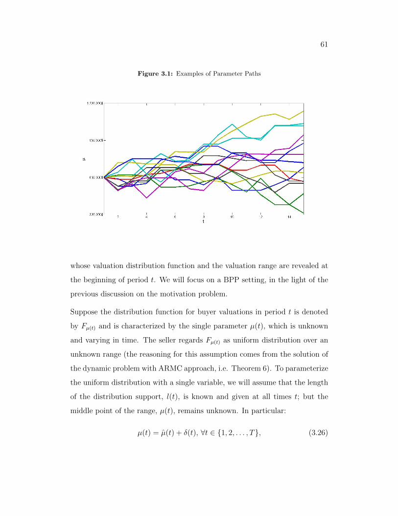
61
Figure 3.1: Examples of Parameter Paths
whose valuation distribution function and the valuation range are revealed at
the beginning of period t. We will focus on a BPP setting, in the light of the
previous discussion on the motivation problem.
Suppose the distribution function for buyer valuations in period t is denoted
by Fµ(t) and is characterized by the single parameter µ(t), which is unknown
and varying in time. The seller regards Fµ(t) as uniform distribution over an
unknown range (the reasoning for this assumption comes from the solution of
the dynamic problem with ARMC approach, i.e. Theorem 6). To parameterize
the uniform distribution with a single variable, we will assume that the length
of the distribution support, l(t), is known and given at all times t; but the
middle point of the range, µ(t), remains unknown. In particular:
µ(t) = µ(t) + δ(t), ∀t ∈ {1, 2, . . . , T}, (3.26)
62
where µ(t) is the forecasted value of the parameter and δ(t) is the unknown
noise factor. Hence, given µ(t), the seller regards the pdf of the buyer valua-
tions as:
fµ(t)(vb) :=
1l(t)
if µ(t)− l(t)2≤ vb ≤ µ(t) + l(t)
2
0 otherwise(3.27)
We make no distributional assumptions regarding δ, except that it lies in a
basic compact algebraic set ∆. This approach gives us more freedom than a
classical stochastic optimization model which often requires uncertainty factors
to be independent across time periods.
As the buyers also regard the seller’s valuation as uniformly distributed in its
given range, they bid according to the uniform bidding function b(vb) = vb2
+ ¯vs2
(which follows from the equilibrium bidding function of the one-to-one BPP
game).
For simplicity, we will pursue the analysis on the example problem stated
above.
If we resize the problem by dividing all monetary values by $300K, and carry
the analysis to a fluid setting, we obtain the following robust optimization
problem:
max{st,t=1,...15}
[15∑t=1
100
4((1.5 +
t∑i=1
δ(t))2 − 4s2t )] (3.28)
subject to 10015∑t=1
((1.5 +t∑i=1
δ(t))− 2st) ≤ at ∀t, (3.29)
15∑t=1
at ≤ 375 a.s.∀t (3.30)
−0.2 ≤ δ(t) ≤ 0.2, ∀t. (3.31)
63
which takes the following form, if we would like to make the objective function
independent of noise factors:
max{st,t=1,...15}
z (3.32)
subject to z ≤ [15∑t=1
100
4((1.5 +
t∑i=1
δ(i))2 − 4s2t )], (3.33)
100((1.5 +t∑i=1
δ(i))− 2st) ≤ at ∀t, (3.34)
15∑t=1
at ≤ 375 a.s.∀t (3.35)
−0.2 ≤ δ(t) ≤ 0.2, at ≥ 0, ∀t. (3.36)
which is an uncertain quadratically-constrained (QC) problem. This class of
problems is analyzed in great detail by many researchers, including A. Ben-Tal
and Roos (2002), who build an SDP which approximates the NP-hard robust
counterpart, and Goldfarb and Iyengar (2003) who reformulate the uncertain
QC problem as an SOCP problem and solve the latter. Although the solu-
tion methodologies proposed in these papers require much less computational
effort than solving the original problem, the main problem with the above
formulation is that it essentially leads to an open-loop solution (i.e. a pricing
policy st that does not make use of the past disturbances), therefore yielding
conservative results for practical use.
However, the hope is that, rather than open-loop policies that do not take
into account the system dynamics, some simple but tractable functional forms
might be sufficient for good performances, if not for optimality. “Affine poli-
cies” of past disturbances, i.e. pricing policies of the form: st = mt +∑ti=1Bt,iδ(i), could be one such policy. This approach is not new in the
literature. It has been originally advocated in the context of stochastic pro-
64
gramming (see Garstka and J.-B.Wets (1974), and references therein), where
such policies are known as decision rules. More recently, the idea has received
renewed interest in robust optimization (A. Ben-Tal and Nemirovski (2004)),
and has been extended to various contexts for solving specific types of opti-
mization problems, which vary from linear and quadratic programs (A. Ben-Tal
and Nemirovski (2005), Kerrigan and Maciejowski (2004)) to conic and semi-
definite (A. Ben-Tal and Nemirovski (2005), Bertsimas and Brown (2007)).
The following formulation of D. Bertsimas and Parrilo (2010) which is mo-
tivated by the inventory replenishment problems in uncertain environments
seems to be closest to our case. The authors consider a one-dimensional, dis-
crete, linear, time-varying dynamical system:
xk+1 = αkxk + βkuk + γkwk
where αk, βk, γk are known scalars, the initial state x1 is specified, wk’s are
bounded (wk ∈ Wk) random disturbances, and the goal is to find the controls
uk’s that obey the constraints uk ∈ Lk, Uk, for known and fixed values Lk, Uk,
and minimizing the following Bellman equation:
Jk(xk) = minLk≤uk≤Uk
[ckuk + maxwk∈Wk
[hk(xk + uk + wk) + Jk+1(xk + uk + wk)]]
where the function hk : R → R ∪ {∞} is convex and coercive; ck’s fixed and
known.
Note that our problem can almost be expressed in the same way as the above
system. In particular, denoting xt as the current inventory level of the seller,
st as the controls and δ(t) as the noise factors, the dynamic system equation
becomes:
xt+1 = xt − (µ(t) + 0.5l(t) + δ(t)− 2st)
65
and the Bellman equation takes the form:
Jk(xk) = minLk≤sk≤Uk
[ maxδk∈∆k
[Λk
l(k)((sk)
2 − (s∗k(xk))2) + Jk+1(xk + uk + wk)]]
where Lk = min{vs, 0.5Λk(µ(k) + 0.5l(k) + δ(k) +¯vs − xk
l(t))}, Uk = 0.5(µ(k) +
0.5l(k)+δ(k)+¯vs) and s∗k(xk) =
[(∑T
t=k Λtµ(t)+0.5l(t)
l(t))−xk
]/(2∑T
t=kΛt
l(t))+0.5
¯vs.
Clearly, in our setting, Lk, Uk are not known in advance and are revealed
during the course of time, and ck = 0, ∀k. But the main difference between
the two settings arises from the fact that in our problem, hk(.) function is a
function of “future” noise factors as clear in the definition of s∗k(xk). Moreover,
since the seller cannot sell more than her capacity, there are linear constraints
that couple controls st across different time steps.
D. Bertsimas and Parrilo (2010) were able to show that the optimal controls
in the above problem are affine functions of the past disturbances. However,
they also show that the optimality of affine policies is easily violated even
when the problem assumptions are relaxed slightly. For instance, they show
that optimality no longer holds when there exist linear constraints coupling
the controls ut across different time-steps, which is exactly the case in our
problem due to the capacity constraints. Hence, in our problem, affine policies
are no longer optimal, but hopefully yield results that are close to optimal.
Moreover, we have an additional structural support in the favor of using affine
policies. To see this, let us take a step back and consider the deterministic
problem. The form of the optimal pricing policy in the deterministic problem
is given in the following Proposition.
Proposition 2. If µ path is known at t = 1 (i.e. δ is known), the optimal
bidding function of the seller having valuation vs in a dynamic negotiation
66
game under BPP setting is given by:
st(vs) = max{b∗(v0b ), vs}, ∀t ∈ {1, 2, . . . , T}
where v0b satisfies:
∑Tt=1 Λt
∫ µ(t)+0.5l(t)
v0b
fµ(t)(vb)dvb = C.
Hence, the optimal clairvoyant policy is a stationary policy where the optimal
bid is given by:
s∗t (vs) = max{vs,
[∑Tt=1 Λt
µ(t)+0.5l(t)l(t)
]− C
2∑T
t=1Λt
l(t)
+ ¯vs2}, ∀t,
when the buyer valuations are uniform. This policy can also be written in
feedback form:
s∗t (vs) = max{vs,∑T
t′=t Λt′(µ(t′)+0.5l(t′)
l(t′))− x(t)
2∑T
t′=tΛt′l(t′)
+ ¯vs2}, ∀t.
where x(t) is the inventory amount at the beginning of period t. That is, given
the µ path, the optimal policy assumes the following feedback form (provided
that s∗t ≥ vs):
s∗t = At +Btx(t) +∑i≥t
Ci,tµ(i) (3.37)
for some known coefficients At, Bt and Ci,t, ∀t.
Thus, inspired by the optimal policy of the deterministic problem, a candidate
closed-loop policy for the stochastic problem could be defined as:
st = At +Btx(t) + Ct,tµ(t) +∑i>t
Ci,t(µ(i) + E[δ(i)]) (3.38)
for some appropriate constants At, Bt and Ci,t, ∀t, ∀i > t.
However, optimizing over the coefficients At, Bt and Ci,t violates the convex
nature of the maximum regret minimization problem (3.32)-(3.36), since x(t)
67
is dependent on si, i = 1, 2, . . . , t − 1, ∀t. Fortunately, noting that both x(t)
and µ(t) are functions of the past noise factors δ(i), i ≤ t; it is possible to
recover the form (3.38) by defining the optimal pricing policy s as an affine
function of the past uncertainties:
Proposition 3. Defining:
st = mt +t∑
j=1
Bt,jδ(j) (3.39)
the formulation (3.38) can be recovered.
(Proof in Appendix B.4.) The proof simply follows from observing that if the
seller bid is defined as in (3.39), the current capacity x(t) can be expressed as
an affine function of previous noise factors δ(j), j ≤ t, in a uniform distribution
setting. Thus, the equivalence of the two formulations follows.
However, the opposite of this claim is not true, i.e. it is not possible to recover
equations (3.39) by (3.38). That is because the degree of freedom is larger for
the set of equations (3.39) (i.e. given the values of mt and Bt,i, ∀t, i ≤ t, there
are more than one solution for At, Bt, Ci,t, ∀t, i > t). To see this, consider the
simplest case, T=2. We know that for any given δ path, the feedback heuristic
pricing policy can be expressed as:
s1,f = A1 +B1x1 + C11δ(1)
s2,f = A2 +B2(x1 − (µ(1) + 0.5l(1) + δ(1)− 2s1,f )) + C22δ(2)
The closed-loop heuristic policy, on the other hand, is expressed as:
s1,c = m1 +K11δ(1)
s2,c = m2 +K21δ(1) +K22δ(2)
68
If si,c = si,c, i = 1, 2 holds, for any given values of A1, B1, C11 and C22, it can
be shown that:
m1 = A1 +B1x1
m2 = A2 +B2x1 −B2(µ(1) + 0.5l(1)) + 2B2A1 + 2B2B1x1
K11 = C11
K21 = −B2 + 2B2C11
K22 = C22
But since the degree of freedom is larger for the second set of equations, it is
not possible to trace back A1, A2 and B1 given the values of m1, m2, K11, K21
and K22 (i.e. there are more than 1 possible solution for these variables). The
case for T > 2 is similar.
Hence, supported by previous research and the structural form of optimal
policy in the deterministic problem, we confine our search to affine pricing
policies. On the example case, the formulation becomes as follows:
max{mt,Bt,i,t=1,...15,i=1,...,t}
z
subject to z ≤ 100
4[
15∑t=1
((1.5 +t∑i=1
δ(i))2 − 4s2t )]
100((1.5 +t∑i=1
δ(i))− 2st) ≤ at ∀t,
15∑t=1
at ≤ 375 a.s.∀t
st = mt +t∑i=1
Bt,iδ(t)∀t
−0.2 ≤ δ(t) ≤ 0.2, at ≥ 0, ∀t.
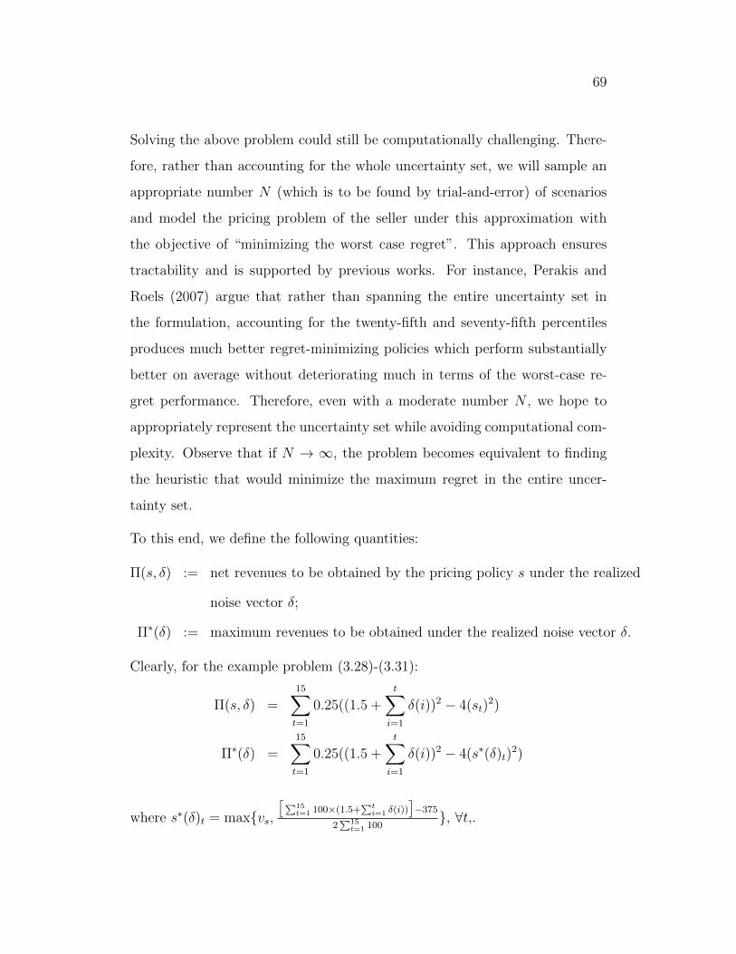
69
Solving the above problem could still be computationally challenging. There-
fore, rather than accounting for the whole uncertainty set, we will sample an
appropriate number N (which is to be found by trial-and-error) of scenarios
and model the pricing problem of the seller under this approximation with
the objective of “minimizing the worst case regret”. This approach ensures
tractability and is supported by previous works. For instance, Perakis and
Roels (2007) argue that rather than spanning the entire uncertainty set in
the formulation, accounting for the twenty-fifth and seventy-fifth percentiles
produces much better regret-minimizing policies which perform substantially
better on average without deteriorating much in terms of the worst-case re-
gret performance. Therefore, even with a moderate number N , we hope to
appropriately represent the uncertainty set while avoiding computational com-
plexity. Observe that if N → ∞, the problem becomes equivalent to finding
the heuristic that would minimize the maximum regret in the entire uncer-
tainty set.
To this end, we define the following quantities:
Π(s, δ) := net revenues to be obtained by the pricing policy s under the realized
noise vector δ;
Π∗(δ) := maximum revenues to be obtained under the realized noise vector δ.
Clearly, for the example problem (3.28)-(3.31):
Π(s, δ) =15∑t=1
0.25((1.5 +t∑i=1
δ(i))2 − 4(st)2)
Π∗(δ) =15∑t=1
0.25((1.5 +t∑i=1
δ(i))2 − 4(s∗(δ)t)2)
where s∗(δ)t = max{vs,[∑15
t=1 100×(1.5+∑t
i=1 δ(i))]−375
2∑15
t=1 100}, ∀t,.
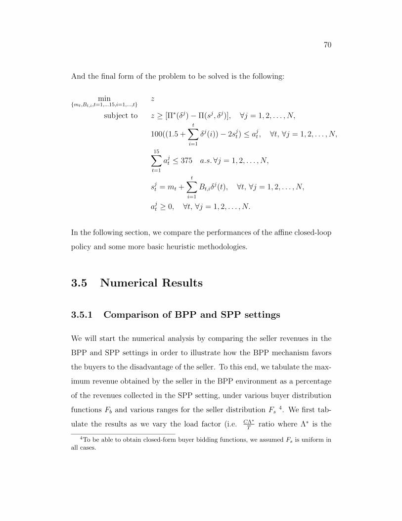
70
And the final form of the problem to be solved is the following:
min{mt,Bt,i,t=1,...15,i=1,...,t}
z
subject to z ≥ [Π∗(δj)− Π(sj, δj)], ∀j = 1, 2, . . . , N,
100((1.5 +t∑i=1
δj(i))− 2sjt) ≤ ajt , ∀t, ∀j = 1, 2, . . . , N,
15∑t=1
ajt ≤ 375 a.s.∀j = 1, 2, . . . , N,
sjt = mt +t∑i=1
Bt,iδj(t), ∀t, ∀j = 1, 2, . . . , N,
ajt ≥ 0, ∀t, ∀j = 1, 2, . . . , N.
In the following section, we compare the performances of the affine closed-loop
policy and some more basic heuristic methodologies.
3.5 Numerical Results
3.5.1 Comparison of BPP and SPP settings
We will start the numerical analysis by comparing the seller revenues in the
BPP and SPP settings in order to illustrate how the BPP mechanism favors
the buyers to the disadvantage of the seller. To this end, we tabulate the max-
imum revenue obtained by the seller in the BPP environment as a percentage
of the revenues collected in the SPP setting, under various buyer distribution
functions Fb and various ranges for the seller distribution Fs4. We first tab-
ulate the results as we vary the load factor (i.e. CΛ∗
Tratio where Λ∗ is the
4To be able to obtain closed-form buyer bidding functions, we assumed Fs is uniform inall cases.
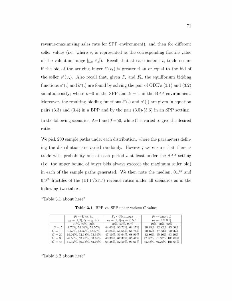
71
revenue-maximizing sales rate for SPP environment), and then for different
seller values (i.e. where vs is represented as the corresponding fractile value
of the valuation range [¯vs, vs]). Recall that at each instant t, trade occurs
if the bid of the arriving buyer b∗(vb) is greater than or equal to the bid of
the seller s∗(vs). Also recall that, given Fs and Fb, the equilibrium bidding
functions s∗(.) and b∗(.) are found by solving the pair of ODE’s (3.1) and (3.2)
simultaneously; where k=0 in the SPP and k = 1 in the BPP environment.
Moreover, the resulting bidding functions b∗(.) and s∗(.) are given in equation
pairs (3.3) and (3.4) in a BPP and by the pair (3.5)-(3.6) in an SPP setting.
In the following scenarios, Λ=1 and T=50, while C is varied to give the desired
ratio.
We pick 200 sample paths under each distribution, where the parameters defin-
ing the distribution are varied randomly. However, we ensure that there is
trade with probability one at each period t at least under the SPP setting
(i.e. the upper bound of buyer bids always exceeds the maximum seller bid)
in each of the sample paths generated. We then note the median, 0.1th and
0.9th fractiles of the (BPP/SPP) revenue ratios under all scenarios as in the
following two tables.
“Table 3.1 about here”
Table 3.1: BPP vs. SPP under various C values
Fb ∼ U[¯vb, vb] Fb ∼ N(µb, σb) Fb ∼ exp(µb)
¯vb ∼ [1, 3], vb =
¯vb + 2 µb ∼ [1, 3]σb ∼ [0.5, 1] µb ∼ [0.2, 0.8]
10%, 50%, 90% 10%, 50%, 90% 10%, 50%, 90%C = 5 4.76%, 51.32%, 53.55% 44.63%, 56.72%, 64.17% 20.45%, 32.82%, 43.00%C = 10 9.52%, 51.32%, 53.55% 43.85%, 54.65%, 61.76% 20.45%, 37.33%, 60.26%C = 20 19.04%, 52.18%, 53.39% 47.10%, 56.64%, 68.99% 32.86%, 65.16%, 93.40%C = 30 28.56%, 53.42%, 63.18% 49.38%, 67.32%, 85.47% 47.90%, 81.50%, 103.02%C = 45 41.32%, 59.13%, 82.16% 65.38%, 82.59%, 96.61% 55.58%, 86.29%, 106.04%
“Table 3.2 about here”
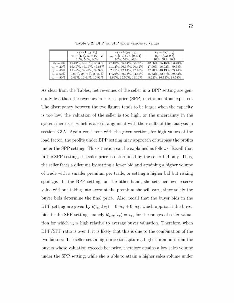
72
Table 3.2: BPP vs. SPP under various vs values
Fb ∼ U[¯vb, vb] Fb ∼ N(µb, σb) Fb ∼ exp(µb)
¯vb ∼ [1, 3], vb =
¯vb + 2 µb ∼ [1, 3]σb ∼ [0.5, 1] µb ∼ [0.2, 0.8]
10%, 50%, 90% 10%, 50%, 90% 10%, 50%, 90%vs = 0% 19.04%, 52.18%, 53.39% 47.10%, 56.64%, 68.99% 32.86%, 65.16%, 93.40%vs = 20% 16.49%, 46.15%, 46.88% 41.42%, 50.97%, 60.42% 27.90%, 56.92%, 79.35%vs = 40% 13.49%, 38.44%, 38.92% 32.41%, 42.14%, 47.93% 22.20%, 46.19%, 59.74%vs = 60% 9.89%, 28.74%, 29.87% 17.79%, 30.03%, 34.57% 15.63%, 32.87%, 39.53%vs = 80% 5.49%, 16.44%, 16.91% 4.96%, 15.50%, 19.16% 8.22%, 16.74%, 19.58%
As clear from the Tables, net revenues of the seller in a BPP setting are gen-
erally less than the revenues in the list price (SPP) environment as expected.
The discrepancy between the two figures tends to be larger when the capacity
is too low, the valuation of the seller is too high, or the uncertainty in the
system increases; which is also in alignment with the results of the analysis in
section 3.3.5. Again consistent with the given section, for high values of the
load factor, the profits under BPP setting may approach or surpass the profits
under the SPP setting. This situation can be explained as follows: Recall that
in the SPP setting, the sales price is determined by the seller bid only. Thus,
the seller faces a dilemma by setting a lower bid and attaining a higher volume
of trade with a smaller premium per trade; or setting a higher bid but risking
spoilage. In the BPP setting, on the other hand, she sets her own reserve
value without taking into account the premium she will earn, since solely the
buyer bids determine the final price. Also, recall that the buyer bids in the
BPP setting are given by b∗BPP (vb) = 0.5¯vs + 0.5vb, which approach the buyer
bids in the SPP setting, namely b∗SPP (vb) = vb, for the ranges of seller valua-
tion for which¯vs is high relative to average buyer valuation. Therefore, when
BPP/SPP ratio is over 1, it is likely that this is due to the combination of the
two factors: The seller sets a high price to capture a higher premium from the
buyers whose valuation exceeds her price, therefore attains a low sales volume
under the SPP setting; while she is able to attain a higher sales volume under
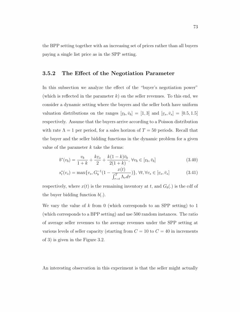
73
the BPP setting together with an increasing set of prices rather than all buyers
paying a single list price as in the SPP setting.
3.5.2 The Effect of the Negotiation Parameter
In this subsection we analyze the effect of the “buyer’s negotiation power”
(which is reflected in the parameter k) on the seller revenues. To this end, we
consider a dynamic setting where the buyers and the seller both have uniform
valuation distributions on the ranges [¯vb, vb] = [1, 3] and [
¯vs, vs] = [0.5, 1.5]
respectively. Assume that the buyers arrive according to a Poisson distribution
with rate Λ = 1 per period, for a sales horizon of T = 50 periods. Recall that
the buyer and the seller bidding functions in the dynamic problem for a given
value of the parameter k take the forms:
b∗(vb) =vb
1 + k+k¯vs2
+k(1− k)vb2(1 + k)
, ∀vb ∈ [¯vb, vb] (3.40)
s∗t (vs) = max{vs, G−1b (1− x(t)∫ T
τ=tΛτdτ
)}, ∀t,∀vs ∈ [¯vs, vs] (3.41)
respectively, where x(t) is the remaining inventory at t, and Gb(.) is the cdf of
the buyer bidding function b(.).
We vary the value of k from 0 (which corresponds to an SPP setting) to 1
(which corresponds to a BPP setting) and use 500 random instances. The ratio
of average seller revenues to the average revenues under the SPP setting at
various levels of seller capacity (starting from C = 10 to C = 40 in increments
of 3) is given in the Figure 3.2.
An interesting observation in this experiment is that the seller might actually
74
Figure 3.2: Seller revenues (as a percentage of revenue at k = 0) for various k and Cvalues
benefit from a slight shift in negotiation power for higher load factor values,
CΛT
. This is mainly due to the fact that the buyer bids might first increase
and then decrease in k for lower-valued buyers (For instance, take a buyer
with vb = 1.2. His bid will be equivalent to b(vb) = vb = 1.2 for k = 0;
b(vb) = vb1.2
+ 0.2×0.52
+ 0.2×0.8×32×1.2
= 1.25 for k = 0.2, and b(vb) = vb2
+ 0.52
= 0.85
for k = 1). As the load factor increases, it is more prevalent to accept lower-
valued buyers, who now bid highest at moderate values of k rather than at
k = 0 or at k = 1. This observation is also consistent with the results of the
previous subsection which suggests that the seller can also do as good or better
under BPP setting than under the SPP setting if she has abundant capacity.
75
3.5.3 An Analysis about the Effect of Uniform
Distribution Assumption
Next, we would like to investigate the seller’s loss when she does not have the
real distribution information and assumes that the buyers’ valuations are dis-
tributed uniformly in their range, which is a natural conclusion of the ARMC
approach. Our experiments contrast the revenues obtained by the seller in the
“no distribution information” setting to the revenues in the “full-information”
setting. To this end, consider the revenue maximization problem of a seller
who wants to sell a number of units over T=15 time periods, where the market
size is Poisson with rate Λ=100 per period.
We restricted the buyer valuations to belong in the range [¯vb, vb] for each
distribution in each period t, t ∈ {1, 2, . . . , 15}. For the Normal and Gumbel
distributions, we extracted the mean as the midpoint of the range and selected
the standard deviation σ by assuming that the range is equal to ±3σ. For the
exponential distribution we assumed that the valuation of a typical consumer
is given by¯vb + w where w is exponentially distributed in [0, vb −
¯vb] and its
rate parameter µ is selected so that the probability that w lies in that range is
99.5% (this is consistent with the ±3σ assumption of the Normal distribution).
In each test case, we assumed that the buyers bid believing that the seller’s
valuation distribution is uniform in the range [¯vs, vs] = [$750K, $2000K]; which
induces a buyer bidding function b∗(vb) = min{vb, 0.5vb + 0.5¯vs}.
The sets of results summarized in Tables 3.3-3.4 illustrate the performance of
the policy under uniform distribution assumption in a variety of settings as
we varied the range of the WtP distribution, the inventory of the seller, and
also the seller valuation. In Table 3.3, the seller’s valuation is assumed to be
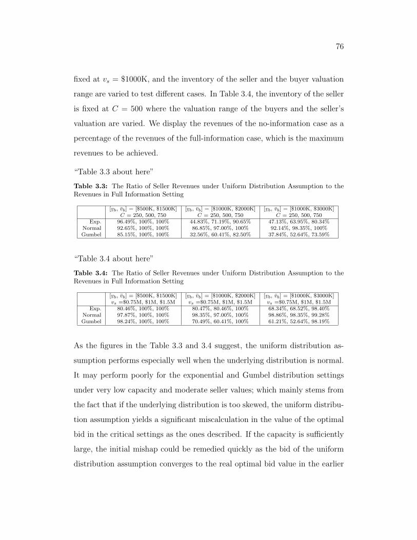
76
fixed at vs = $1000K, and the inventory of the seller and the buyer valuation
range are varied to test different cases. In Table 3.4, the inventory of the seller
is fixed at C = 500 where the valuation range of the buyers and the seller’s
valuation are varied. We display the revenues of the no-information case as a
percentage of the revenues of the full-information case, which is the maximum
revenues to be achieved.
“Table 3.3 about here”
Table 3.3: The Ratio of Seller Revenues under Uniform Distribution Assumption to theRevenues in Full Information Setting
[¯vb, vb] = [$500K, $1500K] [
¯vb, vb] = [$1000K, $2000K] [
¯vb, vb] = [$1000K, $3000K]
C = 250, 500, 750 C = 250, 500, 750 C = 250, 500, 750Exp. 96.49%, 100%, 100% 44.83%, 71.19%, 90.65% 47.13%, 63.95%, 80.34%
Normal 92.65%, 100%, 100% 86.85%, 97.00%, 100% 92.14%, 98.35%, 100%Gumbel 85.15%, 100%, 100% 32.56%, 60.41%, 82.50% 37.84%, 52.64%, 73.59%
“Table 3.4 about here”
Table 3.4: The Ratio of Seller Revenues under Uniform Distribution Assumption to theRevenues in Full Information Setting
[¯vb, vb] = [$500K, $1500K] [
¯vb, vb] = [$1000K, $2000K] [
¯vb, vb] = [$1000K, $3000K]
vs =$0.75M, $1M, $1.5M vs =$0.75M, $1M, $1.5M vs =$0.75M, $1M, $1.5MExp. 80.46%, 100%, 100% 80.47%, 80.46%, 100% 68.34%, 68.52%, 98.40%
Normal 97.87%, 100%, 100% 98.35%, 97.00%, 100% 98.86%, 98.35%, 99.28%Gumbel 98.24%, 100%, 100% 70.49%, 60.41%, 100% 61.21%, 52.64%, 98.19%
As the figures in the Table 3.3 and 3.4 suggest, the uniform distribution as-
sumption performs especially well when the underlying distribution is normal.
It may perform poorly for the exponential and Gumbel distribution settings
under very low capacity and moderate seller values; which mainly stems from
the fact that if the underlying distribution is too skewed, the uniform distribu-
tion assumption yields a significant miscalculation in the value of the optimal
bid in the critical settings as the ones described. If the capacity is sufficiently
large, the initial mishap could be remedied quickly as the bid of the uniform
distribution assumption converges to the real optimal bid value in the earlier
77
periods of the sales horizon, hence resulting in low revenue loss. If the seller
valuation is too large, again the two revenue figures are equivalent or very
close to each other, which is because in this case the optimal bid is the seller
valuation itself regardless of the underlying distribution.
3.5.4 Stochastic Dynamic BPP Problem
Example 1 (continued): Recall the problem of a seller who has C=375
units to sell over T=15 time periods, where the market size is Poisson with
rate Λ=100 per period. The buyer valuation distribution is uniform on the
range [µ(t)− $300K,µ(t) + $300K], with the parameter µ changing according
to the formula:
µ(t) = µ(t− 1) + δ(t)
with µ(1)=$600K, where δ(t) is the random drift given by:
δ(t) =
−d, w.p 0.4
0, w.p 0.2
d, w.p 0.4
∀t
where d ∼ U[0, $120K]. Suppose the buyers bid according to the bidding
function b∗(vb) = 0.5vb. In the base case, assume we do not account for the
salvage value of the seller, hence vs = 0.
We solve the scenario-based optimization problem for various seller valuation
(vs), capacity (C), and noise-size (d := |δ|) values with N=150 scenarios; and
compare the results with the simple “expected value (EV)” heuristic, where all
stochastic variables in the problem are assumed to take their expected values,
and with the solution of the uncertain QC-formulation given in (3.32)-(3.36),
which we call “uncertain QC (UQC)” solution. For all policies, we compute
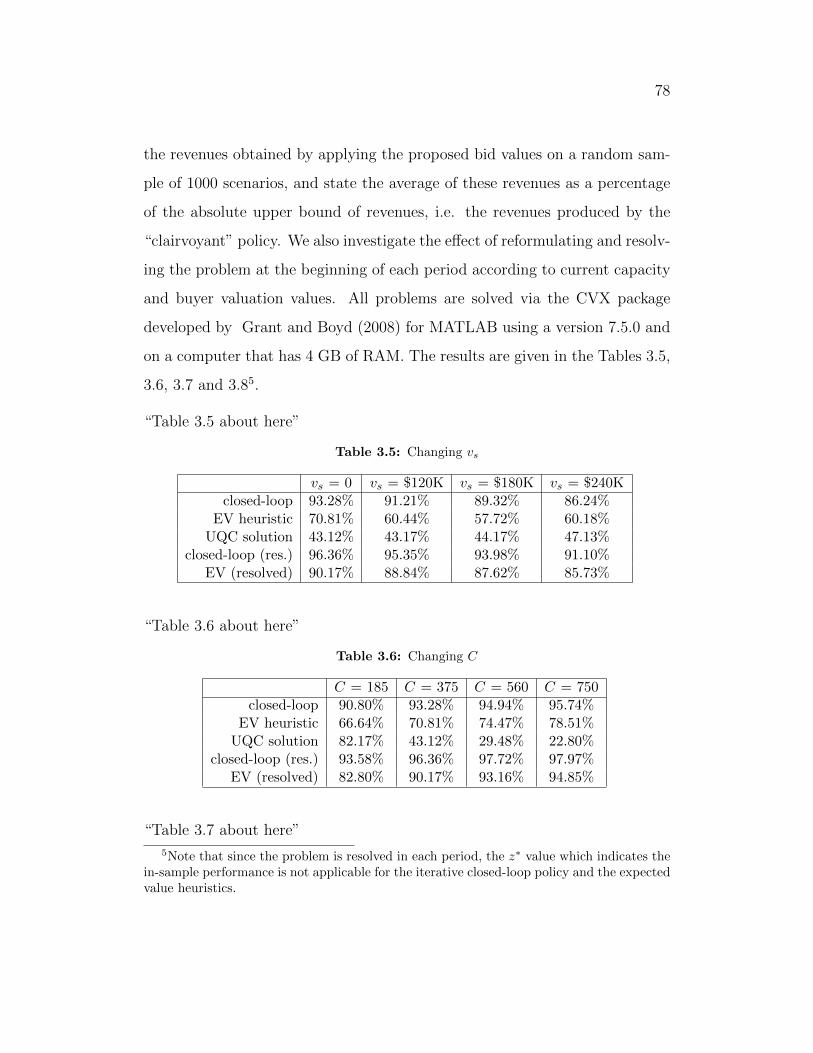
78
the revenues obtained by applying the proposed bid values on a random sam-
ple of 1000 scenarios, and state the average of these revenues as a percentage
of the absolute upper bound of revenues, i.e. the revenues produced by the
“clairvoyant” policy. We also investigate the effect of reformulating and resolv-
ing the problem at the beginning of each period according to current capacity
and buyer valuation values. All problems are solved via the CVX package
developed by Grant and Boyd (2008) for MATLAB using a version 7.5.0 and
on a computer that has 4 GB of RAM. The results are given in the Tables 3.5,
3.6, 3.7 and 3.85.
“Table 3.5 about here”
Table 3.5: Changing vs
vs = 0 vs = $120K vs = $180K vs = $240Kclosed-loop 93.28% 91.21% 89.32% 86.24%
EV heuristic 70.81% 60.44% 57.72% 60.18%UQC solution 43.12% 43.17% 44.17% 47.13%
closed-loop (res.) 96.36% 95.35% 93.98% 91.10%EV (resolved) 90.17% 88.84% 87.62% 85.73%
“Table 3.6 about here”
Table 3.6: Changing C
C = 185 C = 375 C = 560 C = 750closed-loop 90.80% 93.28% 94.94% 95.74%
EV heuristic 66.64% 70.81% 74.47% 78.51%UQC solution 82.17% 43.12% 29.48% 22.80%
closed-loop (res.) 93.58% 96.36% 97.72% 97.97%EV (resolved) 82.80% 90.17% 93.16% 94.85%
“Table 3.7 about here”
5Note that since the problem is resolved in each period, the z∗ value which indicates thein-sample performance is not applicable for the iterative closed-loop policy and the expectedvalue heuristics.
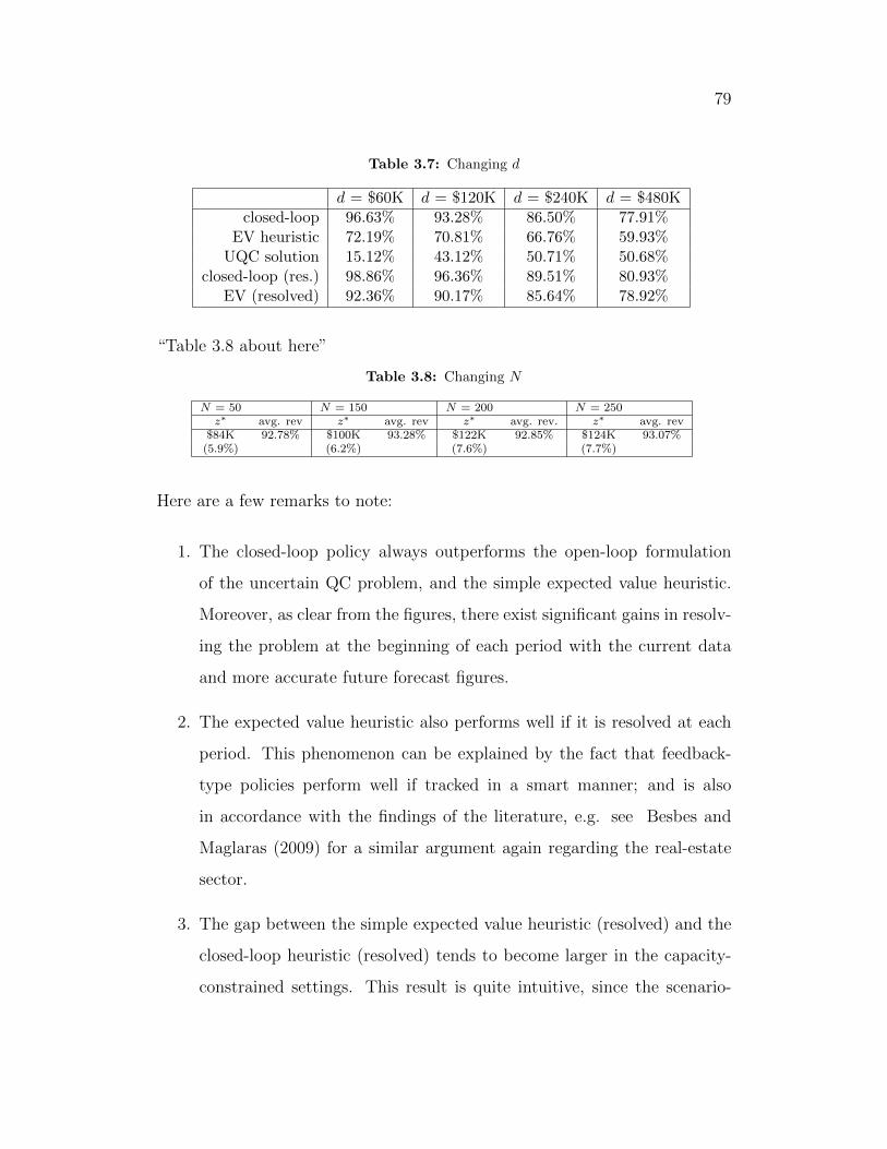
79
Table 3.7: Changing d
d = $60K d = $120K d = $240K d = $480Kclosed-loop 96.63% 93.28% 86.50% 77.91%
EV heuristic 72.19% 70.81% 66.76% 59.93%UQC solution 15.12% 43.12% 50.71% 50.68%
closed-loop (res.) 98.86% 96.36% 89.51% 80.93%EV (resolved) 92.36% 90.17% 85.64% 78.92%
“Table 3.8 about here”
Table 3.8: Changing N
N = 50 N = 150 N = 200 N = 250z∗ avg. rev z∗ avg. rev z∗ avg. rev. z∗ avg. rev
$84K 92.78% $100K 93.28% $122K 92.85% $124K 93.07%(5.9%) (6.2%) (7.6%) (7.7%)
Here are a few remarks to note:
1. The closed-loop policy always outperforms the open-loop formulation
of the uncertain QC problem, and the simple expected value heuristic.
Moreover, as clear from the figures, there exist significant gains in resolv-
ing the problem at the beginning of each period with the current data
and more accurate future forecast figures.
2. The expected value heuristic also performs well if it is resolved at each
period. This phenomenon can be explained by the fact that feedback-
type policies perform well if tracked in a smart manner; and is also
in accordance with the findings of the literature, e.g. see Besbes and
Maglaras (2009) for a similar argument again regarding the real-estate
sector.
3. The gap between the simple expected value heuristic (resolved) and the
closed-loop heuristic (resolved) tends to become larger in the capacity-
constrained settings. This result is quite intuitive, since the scenario-
80
based approach can account for various states of the world and prevent
the inventory from depleting much earlier than the end of the period;
whereas the myopic approach could lead to shortages in most of the
cases.
4. Finally, to see the effect of using a certain number of random scenarios
in the optimization model, we also compute the worst-case regret (z∗)
within the scenarios used in the optimization and state its ratio to the
average optimal revenues of the scenarios used in the model. First, we
observe that the worst case regret value is relatively low with respect
to average revenues in almost all cases. This is also an indication that
the proposed closed-loop formulation does not produce too conservative
results. Second, as seen from the results in the Table 3.8, both the
in-sample (i.e. maximum regret) and out-of-sample (i.e. the revenue
gap in other scenarios) performances of the closed-loop policy do not
change much by increasing the number of random scenarios used in the
optimization problem after a critical number is reached. Moreover, this
critical number of scenarios is expected to be as low as N = 150 for a
problem of the above size.
3.6 Conclusion
In this chapter, we discussed the dynamic negotiation problems, and in par-
ticular the transactions in a buyer’s market. We started with the classical
one-to-one negotiation problem and discussed how it is extended to account
for uncertainty in valuation distributions. Next, we extended our analysis to
capture various situations in the dynamic environment: Starting with formu-
81
lating and solving the deterministic fluid problem, we were able to observe
the structural properties of the optimal pricing policy; which is the stationary
nature of this policy. We were then able to extend the analysis to the problems
with uncertain parameters, and offer tractable and effective solution method-
ologies for real life applications with uncertain and time-varying parameters.
Moreover, we established the theoretical motivation to use uniform distribution
in the situations where the distribution information of the valuation of the op-
ponent party is not readily available; and emphasized the connection between
the dynamic negotiation problems and the revenue management problems.
Our results also offer various avenues of future research: First, there could
be several forms of negotiation problems to be analyzed in a dynamic setting
from the game theoretical perspective we presented. Of these, the games that
involve strategic buyers who could choose their time of purchase is of utmost
interest. Also, the closed-loop formulation we developed or the structural
results we presented regarding the nature of the optimal pricing policies for
the certain set of problems discussed in this work might be inspiring and in-
sightful in the formulation and solution of various other scenario-based robust
optimization problems.
82
Chapter 4
Pricing Problem of a
Monopolist in the Presence of
Investors
4.1 Introduction and Literature Review
In this chapter, we analyze the revenue maximization problem of a seller who
operates in a market where two type of customers exist: the “investors” and
“regular buyers”.
The problem is motivated by the revenue maximization problem of a real-estate
developer who wants to sell a number of units in a market where investors are
prevalent. In this setting, the regular buyers are defined to be the customers
who purchase the units with self-inhabitance purposes whereas investors are
the buyers who purchase the units with the intention of re-selling them again
83
within the sales period of the developer at a higher price, possibly cannibal-
izing some of the developer’s demand. Although in practice, investors in the
real estate market may make purchase or sell decisions upon various financial
factors including their expected rate of return, risk management factors, or
portfolio variance criteria among many others; we do not incorporate financial
details in our formulation. Instead, we focus on the game-theoretical perspec-
tive of the interaction between the developer and the investors. Thus, our
model is applicable to various business settings that include a “pricing game
in a duopoly”.
The price and quantity duopoly games have extensively been studied in the
literature, and various modeling approaches are applicable to these games. For
an extensive review of oligopoly pricing game models, we refer the reader to
Puu and Sushko (2002). Bertrand, Cournot and Stackelberg games are per-
haps among the oldest and the most well-studied models. Various versions
of these models are studied in the literature. For instance, Tasnadi (1999)
expands a Bertrand-Edgeworth duopoly into a two-stage game in which dur-
ing the first stage the firms can select their “rationing rule” that determines
how the market demand is shared between two parties with different prices.
He shows that under certain conditions the efficient rationing rule is an equi-
librium action of the first stage. Birge et al. (1998) address joint capacity
and pricing decisions for two substitutable products where the demands are
uniformly distributed. They later consider the case where each product is
managed by a product manager trying to maximize individual product profits
rather than overall firm profits, and analyze how optimal price and capacity
decisions are affected. There are fundamental differences between the setting
of their paper and of ours: For instance, the capacity level is a strategic deci-
84
sion in their paper whereas it is a problem parameter in our work; and they
restrict their attention to Bertrand and Stackelberg games. Still, if the substi-
tutable products of this paper are thought of as the same type of goods that
are sold by different players, the results are similar. Herk (1993) also considers
a two-stage model of duopolistic capacity choice and subsequent price com-
petition, and shows that consumer switching costs can deter some consumers
from seeking service at a low-price firm that lacks sufficient capacity to serve
the entire market. Moreover, if consumers are approximately risk neutral with
respect to service reliability, then capacity-constrained duopoly competition
has a unique, subgame-perfect equilibrium in which firms choose Cournot ca-
pacities and prices. Deneckere and Peck (1995) consider a two-stage game
in which firms simultaneously select prices and capacities; and the customers
select a firm based on the maximum utility attained, which depends on the
firm’s price-service pair. Similarly, Bansal and Maglaras (2009) study the dy-
namic pricing problem of a monopolist firm in presence of strategic customers
that differ in their valuations and risk preferences, and they show through an
asymptotic analysis that the ‘two-price point’ strategy is near-optimal. The
main difference between this line of research and our work is that the sell-
ing parties in our paper have fixed capacities once the second stage of the
sales period starts, and these capacity levels are observed by the customers
in the market. Thus, in our framework, it is not possible to assume that the
customers base their decisions on maximizing a utility function of expected
service rates. Moreover, the nature of the problem does not align with this
idea, since the real-estate transactions involve expensive items that do not
have the same expected service rate concept as in the daily transactions. We
define the pricing game between the developer and the investors in a way
that potential buyers choose from which vendor to buy according to the price
85
differential between them and their own valuation for the unit.
Having characterized the pricing game between two competing sellers, we later
show that both parties are better off in equilibrium by “cooperating” rather
than “competing”. This is a well-known result of the supply chain and pricing
literature: Federgruen and Bernstein (Bernstein et al. (2002), Bernstein and
Federgruen (2003), Bernstein and Federgruen (2005)) prove the advantages
of centralized decision making process where a single party determines the
quantity replenishment values with the objective of maximizing the overall
profits of the entire supply chain, over the decentralized decision making, where
each agent gives replenishment orders with the objective of maximizing his/her
own profit only. Similarly, Cachon (2003) presents an extensive analysis of
the game between a supplier and a retailer, and shows how different forms
of contracts could be used to lead the retailer to act towards maximizing the
system profits. Contracting schemes have also been used widely in the revenue
management literature to establish some form of a cooperation. For instance,
Gallego and Kou (2008) develop the concept of the “callable products”, which
is based on the idea of selling unused capacity to low-valuation buyers and
re-buying this capacity later in case high-valued demand arises. Similarly,
Gallego and Sahin (2006) show the benefits of options over spot-selling and
forward-selling mechanisms in retail markets.
Our contributions are twofold: First, we formulate and analyze a new pricing
game between two parties where both players have fixed and inflexible capac-
ities. Next, we compare the optimal revenues obtained in this setting with
the revenues of the situation in which, rather than playing a pricing game, the
agents cooperate and establish their prices accordingly. Hence, it is possible to
design various contracting schemes to be able to capture the additional benefits
86
obtained by cooperation, one of which we state and analyze numerically.
The organization of this chapter is as follows: In section 4.2, we formulate
and analyze the problem where each agent makes his/her own price decision
in a two-period model. In this setting, investors purchase a number of units
from the developer in the first period, and resell them in the latter. We start
by characterizing the equilibrium of the game between the developer and the
investors in the latter period; and work our way back to the former period,
where we characterize the revenue maximizing strategy of the developer. In
section 4.3, we analyze the “centralized system” where the pricing decisions
are made by a single party (the developer) and compute the revenues of this
system. In the next section 4.4, we analyze the additional profit opportunities
by centralizing the pricing decisions. Furthermore, based on our analysis of the
previous part, in 4.5 we suggest an easily applicable contracting scheme to be
offered to the investors that leads to an increase in the revenues of both parties,
i.e. a win-win situation. Finally, we conclude by stating further avenues of
research in 4.6.
4.2 The Decentralized Model
In this part, we consider the problem in a two-period setting, where there
exists no cooperation between the agents. We will refer to the two periods
of the problem as t = 0 and t = 1. At t = 0, there are both regular buyers
and investors in the market. At t = 1, all buyers in the market are regular
buyers. In both periods, the willingness-to-pay (WtP) values of the regular
87
buyers are uniformly distributed 1. The WtP values of regular buyers at t = 0
are known to lie within the interval [¯v0, v0] = [0, v0]. The exact range of WtP
distribution at t = 1, which is [¯v1, v1] = [0, v1], is unknown at t = 0 and
revealed before the pricing decisions of t = 1 are made and sales take place.
However, we assume that v1 = v0 + γ for some random variable γ with a
cumulative distribution function G(·) (and a continuous pdf g) on the known
and bounded range [−a, a]. Thus, it is possible to define the unknown support
of WtP distribution of buyers at t = 1 by a single parameter, which is γ.
Finally, the market size of regular buyers at t = 0 is given as Λ0, whereas
the market size at t = 1, Λ1, is again a random variable whose probability
distribution function is f(·) at t = 0 and exact value is only revealed at t = 1.
We will adopt a fluid formulation framework and assume that all buyers are
infinitesimal. Hence, the sales amount at a certain price level takes its expected
value.
The sequence of events in this two-period problem is as follows: At t = 0, the
developer (who will also be referred to as the “seller” interchangeably through-
out the chapter) has C units to sell, and announces a sales price ps0. First,
the regular buyers whose WtP is higher than this price, i.e. a total number
of Dr0 := Λ0
v0−ps0v0
regular buyers, purchase the units. Then the investors, who
base their purchase decision on the expectation of their net revenue at t = 1,
put a deposit payment (dps0 per unit where d is a predetermined constant,
d ∈ (0, 1)) for a total number of Di0 ≤ C −Λ0
v0−ps0v0
units that maximizes their
expected revenues.
We assume that after these transactions occur but before the next sales period
1The uniform distribution argument is based on Chapter 3 where the negotiating partiesassume that their opponents’ valuation is distributed uniformly within its range if no otherdistribution information is available.
88
starts, the information regarding the WtP range of regular buyers at t = 1 (i.e.
the exact value of γ) is revealed. Let us call the time at which this information
is revealed as t = 0.5 to avoid confusion. We assume that this is the time for
the investors to decide what portion of the units they put a down payment
for, Di0, to claim. We assume that all investors act like a single body and
collectively claim qi (qi ≤ Di0) of these units. Then, they pay an additional
amount of qi× (1−d)ps0 to the seller at t = 0.5 and forfeit dps0(Di0− qi). While
they make this decision, the exact value of Λ1 is still unknown.
At t = 1, the value of Λ1 is revealed, and the investors and the developer choose
their respective prices pi1 and ps1 simultaneously. Suppose the developer has qs
units left after the investors claimed qi units. Finally the market demand each
of them observes is calculated as follows: Assume w.l.o.g. that pi1 ≤ ps1. Then,
the minimum WtP value of customers who purchase from the higher-priced
vendor (the developer in this case) is given by:
x(ps1, pi1) = min{ v1 + ps1
2+ (ps1 − pi1), v1} (4.1)
Given x(ps1, pi1), all buyers who have valuations between [pi1, x(ps1, p
i1)] will pur-
chase the units from the lower-price agent (i.e. the investors in this case),
whereas the customers whose valuations lie in the range [x(ps1, pi1), v1] buy from
the agent with the higher price. In other words, the demand the higher-priced
agent observes takes the value Λ1v1−x(ps1,p
i1)
v1, while the demand the lower-priced
agent observes is equivalent to Λ1x(ps1,p
i1)−pi1v1
. Note that as pi1 → ps1, x→ v1+ps12
,
i.e. when the two prices are equivalent, the market demand is split between the
two agents equally; whereas if pi1 << ps1, x = v1 i.e. if the gap between ps1 and
pi1 is considerably large, all buyers in the market prefer the lower-price agent.
The case with ps1 ≤ pi1 is symmetrical and omitted for the sake of brevity.
The higher-valued customers being usually less price-sensitive is a common as-
89
sumption in the literature, and the above model aims to capture this effect. In
other words, provided that there does not exist a considerable price difference
between substitutable alternatives, some high-valued buyers are content with
paying higher prices to be able to acquire the units without spending much
time or effort in the process of searching for cheaper alternatives, whereas the
lower-valued buyers may wait longer in the market to buy at a lower price
later (for an exemplification of this phenomenon, we refer the reader to Su
(2007)). Also note that by using this model, we were able to differentiate be-
tween the buyers who purchase from the lower-priced vendor and those who
purchase from the higher-priced one in a smooth manner. Using a model where
the demand sharply shifts to the lower-priced vendor if his price drops even
slightly below the price of his competitor, as in Tasnadi (1999), might also be
admissible; however it will not carry the smooth nature of Bertrand duopolies
where the demand is linear, increases in the competitor’s price and decreases
in one’s own price.
Figure 4.1 shows the sequence of events.
“Figure 4.1 about here”
4.2.1 The Pricing Problem at t = 1
We start with the problem at t = 1. Define πs1 and πi1 as the profit function
of the seller and the investor respectively at t = 1. Recall that qs and qi are
the inventory values of the developer and the investors respectively at t = 1.
We denote the maximum profit to be obtained by the seller as Πs1(·) and
the maximum profit to be obtained by the investors as Πi1(·). The revenue
maximization problems of the agents at t = 1 can be stated in their general
90
Figure 4.1: Sequence of Events
forms as follows: 2
Πs1(γ,Λ1, qs, qi) = max
ps1πs1(ps1|γ,Λ1, p
i∗1 , qs, qi)
:= maxps1
ps1 min{qs,
Λ1[v1 − x(ps1, p
i∗1 )
v1
1{pi∗1 ≤ps1} +x(pi∗1 , p
s1)− ps1v1
1{pi∗1 ≥ps1}]}
(4.2)
2Although γ is not expressed explicitly in the equations, observe that the revenue func-tions are also functions of γ since it is involved in the definition of v1.
91
Πi1(γ,Λ1, qs, qi) = max
pi1
πi1(pi1|γ,Λ1, ps∗1 , qs, qi)
:= maxpi1
pi1 min{qi,
Λ1[v1 − x(pi1, p
s∗1 )
v1
1{ps∗1 ≤pi1} +x(ps∗1 , p
i1)− pi1v1
1{ps∗1 ≥pi1}]}
(4.3)
where ps∗1 and pi∗1 are the maximizers of Πs1 and Πi
1 respectively. That is, given
the value of Λ1 and their respective inventories, both parties try to select
the best-response price that would bring them the greatest profit under the
optimal price selection of the other party. We do not assume a Stackelberg
game where the one of the players is the leader and the other the follower;
but rather assume that both agents choose prices simultaneously. Hence the
above problems should be solved together and the optimal prices should be
best-responses to each other.
To be able to solve the two problems more easily, we first characterize some
properties of the equilibrium as in the following Theorem.
Theorem 7. If qs < qi, then there is at least an equilibrium in which the
prices are such that ps∗1 ≥ pi∗1 ; and vice versa.
We will prove Theorem 7 by characterizing the equilibrium prices and show
that the claim of the Theorem holds in all cases. To this end, we start by
assuming that Theorem 7 holds. Then, w.l.o.g, for qs < qi, the two revenue
maximization problems simplify to:
Πs1(γ,Λ1, qs, qi) = max
ps1≥pi∗1πs1(ps1|γ,Λ1, p
i∗1 , qs, qi)
= maxps1≥pi∗1
ps1 min{qs,Λ1[
v1 − x(ps1, pi∗1 )
v1
]}
92
Πi1(γ,Λ1, qs, qi) = max
pi1≤ps∗1πi1(pi1|γ,Λ1, p
s∗1 , qs, qi)
= maxpi1≤ps∗1
pi1 min{qi,Λ1[
x(ps∗1 , pi1)− pi1v1
]}
Next, to simplify the two maximization problems even further, observe that
the following Proposition is true (proof in Appendix C.1).
Proposition 4. If prices ps∗1 and pi∗1 (≤ ps∗1 ) constitute an equilibrium of the
pricing game between the developer and the investors, thenv1+ps∗1
2+(ps∗1 −pi∗1 ) ≤
v1.
This proposition allows us to restate x(ps1, pi1) as x(ps1, p
i1) =
v1+ps12
+ (ps1 − pi1).
Then, the above problems simplify to:
Πs1(γ,Λ1, qs, qi) = max
ps1≥pi∗1ps1 min
{qs,Λ1[
v1 − v1+ps12− (ps1 − pi∗1 )
v1
]}
Πi1(γ,Λ1, qs, qi) = max
pi1≤ps∗1pi1 min
{qi,Λ1[
v1+ps∗12
+ (ps∗1 − pi1)− pi1v1
]}
First, we consider the unconstrained problems, i.e. without taking into account
the inventory values qs, qi. These two problems can be expressed as maximizing
the functions φ1(.|pi∗1 ) and φ2(.|ps∗1 ) respectively, where:
φ1(ps1|pi∗1 ) = ps1Λ1[v1 − v1+ps1
2− (ps1 − pi∗1 )
v1
] (4.4)
and
φ2(pi1|ps∗1 ) = pi1Λ1[
v1+ps∗12
+ (ps∗1 − pi1)− pi1v1
] (4.5)
Observe that both functions φ1(.|pi∗1 ) and φ2(.|ps∗1 ) are concave and are max-
imized at p∗s =2pi∗1 +v1
6and p∗i =
v1+3ps∗18
respectively. Thus, the revenue maxi-
mization problems Πs1(γ,Λ1, qs, qi) and Πi
1(γ,Λ1, qs, qi) are maximization prob-
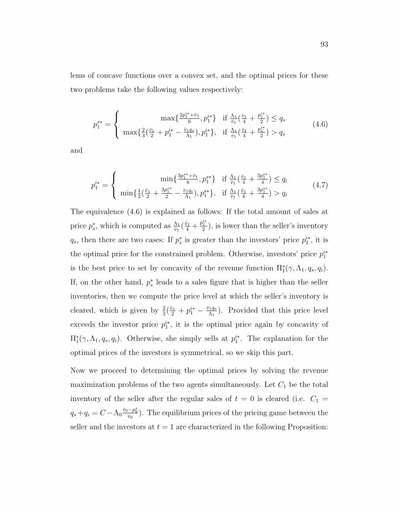
93
lems of concave functions over a convex set, and the optimal prices for these
two problems take the following values respectively:
ps∗1 =
max{2pi∗1 +v1
6, pi∗1 } if Λ1
v1( v1
4+
pi∗12
) ≤ qs
max{23( v1
2+ pi∗1 −
v1qsΛ1
), pi∗1 }, if Λ1
v1( v1
4+
pi∗12
) > qs(4.6)
and
pi∗1 =
min{3ps∗1 +v1
8, ps∗1 } if Λ1
v1( v1
4+
3ps∗14
) ≤ qi
min{12( v1
2+
3ps∗12− v1qi
Λ1), ps∗1 }, if Λ1
v1( v1
4+
3ps∗14
) > qi(4.7)
The equivalence (4.6) is explained as follows: If the total amount of sales at
price p∗s, which is computed as Λ1
v1( v1
4+
pi∗12
), is lower than the seller’s inventory
qs, then there are two cases: If p∗s is greater than the investors’ price pi∗1 , it is
the optimal price for the constrained problem. Otherwise, investors’ price pi∗1
is the best price to set by concavity of the revenue function Πs1(γ,Λ1, qs, qi).
If, on the other hand, p∗s leads to a sales figure that is higher than the seller
inventories, then we compute the price level at which the seller’s inventory is
cleared, which is given by 23( v1
2+ pi∗1 −
v1qsΛ1
). Provided that this price level
exceeds the investor price pi∗1 , it is the optimal price again by concavity of
Πs1(γ,Λ1, qs, qi). Otherwise, she simply sells at pi∗1 . The explanation for the
optimal prices of the investors is symmetrical, so we skip this part.
Now we proceed to determining the optimal prices by solving the revenue
maximization problems of the two agents simultaneously. Let C1 be the total
inventory of the seller after the regular sales of t = 0 is cleared (i.e. C1 =
qs+qi = C−Λ0v0−ps0v0
). The equilibrium prices of the pricing game between the
seller and the investors at t = 1 are characterized in the following Proposition:
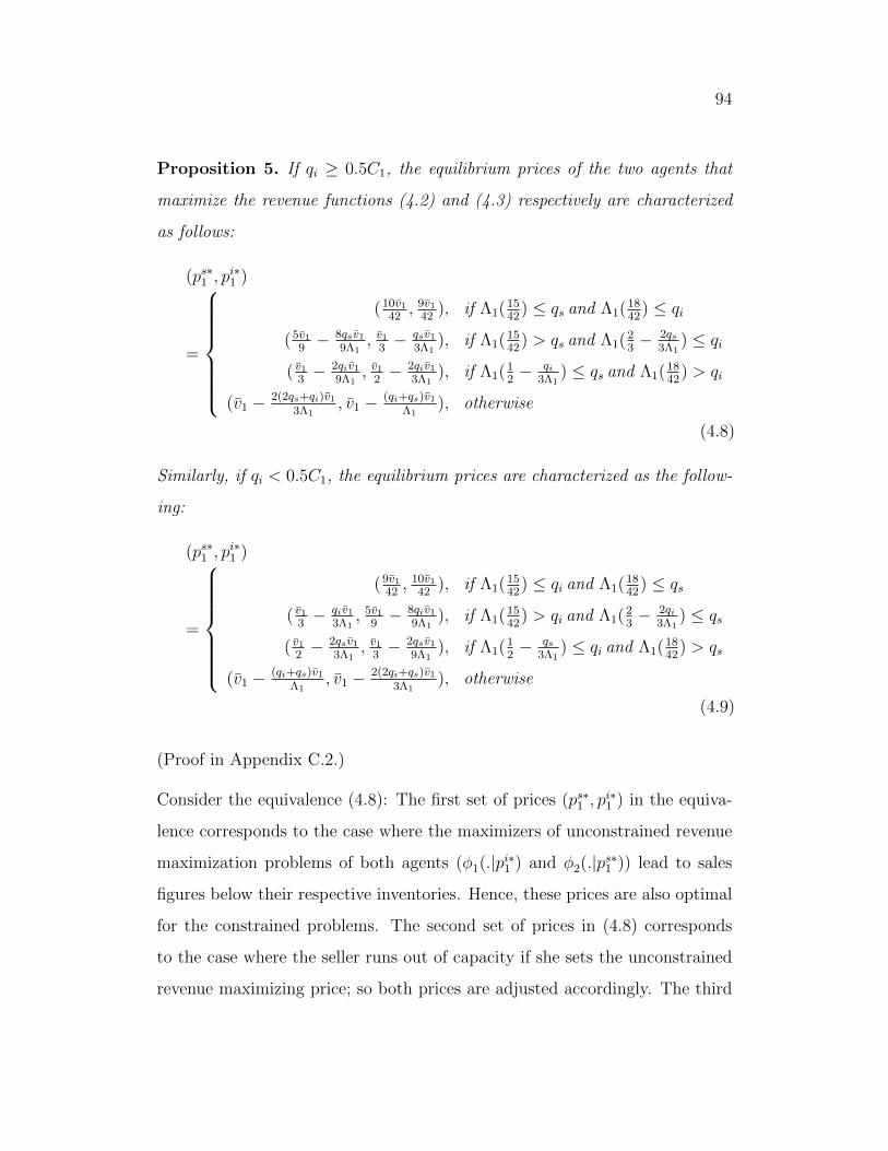
94
Proposition 5. If qi ≥ 0.5C1, the equilibrium prices of the two agents that
maximize the revenue functions (4.2) and (4.3) respectively are characterized
as follows:
(ps∗1 , pi∗1 )
=
(10v1
42, 9v1
42), if Λ1(15
42) ≤ qs and Λ1(18
42) ≤ qi
(5v1
9− 8qsv1
9Λ1, v1
3− qsv1
3Λ1), if Λ1(15
42) > qs and Λ1(2
3− 2qs
3Λ1) ≤ qi
( v1
3− 2qiv1
9Λ1, v1
2− 2qiv1
3Λ1), if Λ1(1
2− qi
3Λ1) ≤ qs and Λ1(18
42) > qi
(v1 − 2(2qs+qi)v1
3Λ1, v1 − (qi+qs)v1
Λ1), otherwise
(4.8)
Similarly, if qi < 0.5C1, the equilibrium prices are characterized as the follow-
ing:
(ps∗1 , pi∗1 )
=
(9v1
42, 10v1
42), if Λ1(15
42) ≤ qi and Λ1(18
42) ≤ qs
( v1
3− qiv1
3Λ1, 5v1
9− 8qiv1
9Λ1), if Λ1(15
42) > qi and Λ1(2
3− 2qi
3Λ1) ≤ qs
( v1
2− 2qsv1
3Λ1, v1
3− 2qsv1
9Λ1), if Λ1(1
2− qs
3Λ1) ≤ qi and Λ1(18
42) > qs
(v1 − (qi+qs)v1
Λ1, v1 − 2(2qi+qs)v1
3Λ1), otherwise
(4.9)
(Proof in Appendix C.2.)
Consider the equivalence (4.8): The first set of prices (ps∗1 , pi∗1 ) in the equiva-
lence corresponds to the case where the maximizers of unconstrained revenue
maximization problems of both agents (φ1(.|pi∗1 ) and φ2(.|ps∗1 )) lead to sales
figures below their respective inventories. Hence, these prices are also optimal
for the constrained problems. The second set of prices in (4.8) corresponds
to the case where the seller runs out of capacity if she sets the unconstrained
revenue maximizing price; so both prices are adjusted accordingly. The third
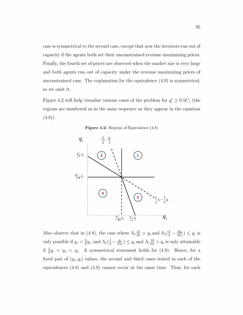
95
case is symmetrical to the second case, except that now the investors run out of
capacity if the agents both set their unconstrained revenue maximizing prices.
Finally, the fourth set of prices are observed when the market size is very large
and both agents run out of capacity under the revenue maximizing prices of
unconstrained case. The explanation for the equivalence (4.9) is symmetrical,
so we omit it.
Figure 4.2 will help visualize various cases of the problem for q∗i ≥ 0.5C1 (the
regions are numbered as in the same sequence as they appear in the equation
(4.8)).
Figure 4.2: Regions of Equivalence (4.8)
Also observe that in (4.8), the case where Λ11542> qs and Λ1(2
3− 2qs
3Λ1) ≤ qi is
only possible if qs <56qi; and Λ1(1
2− qi
3Λ1) ≤ qs and Λ1
1842> qi is only attainable
if 56qi < qs < qi. A symmetrical statement holds for (4.9). Hence, for a
fixed pair of (qs, qi) values, the second and third cases stated in each of the
equivalences (4.8) and (4.9) cannot occur at the same time. Thus, for each
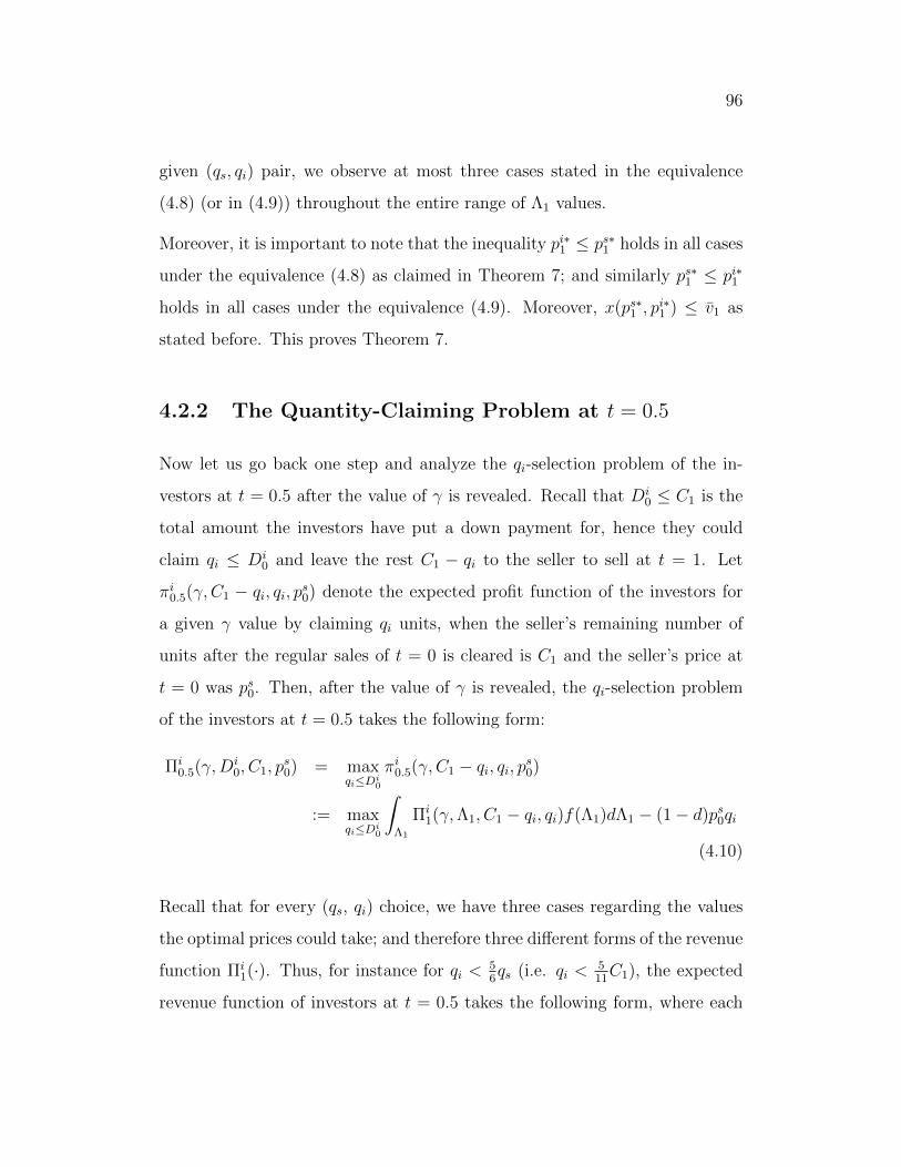
96
given (qs, qi) pair, we observe at most three cases stated in the equivalence
(4.8) (or in (4.9)) throughout the entire range of Λ1 values.
Moreover, it is important to note that the inequality pi∗1 ≤ ps∗1 holds in all cases
under the equivalence (4.8) as claimed in Theorem 7; and similarly ps∗1 ≤ pi∗1
holds in all cases under the equivalence (4.9). Moreover, x(ps∗1 , pi∗1 ) ≤ v1 as
stated before. This proves Theorem 7.
4.2.2 The Quantity-Claiming Problem at t = 0.5
Now let us go back one step and analyze the qi-selection problem of the in-
vestors at t = 0.5 after the value of γ is revealed. Recall that Di0 ≤ C1 is the
total amount the investors have put a down payment for, hence they could
claim qi ≤ Di0 and leave the rest C1 − qi to the seller to sell at t = 1. Let
πi0.5(γ, C1 − qi, qi, ps0) denote the expected profit function of the investors for
a given γ value by claiming qi units, when the seller’s remaining number of
units after the regular sales of t = 0 is cleared is C1 and the seller’s price at
t = 0 was ps0. Then, after the value of γ is revealed, the qi-selection problem
of the investors at t = 0.5 takes the following form:
Πi0.5(γ,Di
0, C1, ps0) = max
qi≤Di0
πi0.5(γ, C1 − qi, qi, ps0)
:= maxqi≤Di
0
∫Λ1
Πi1(γ,Λ1, C1 − qi, qi)f(Λ1)dΛ1 − (1− d)ps0qi
(4.10)
Recall that for every (qs, qi) choice, we have three cases regarding the values
the optimal prices could take; and therefore three different forms of the revenue
function Πi1(·). Thus, for instance for qi <
56qs (i.e. qi <
511C1), the expected
revenue function of investors at t = 0.5 takes the following form, where each
97
integrand corresponds to different ranges of Λ1 values that lead to different
optimal price pairs defined in (4.9):
πi0.5(γ, qs, qi, ps0) =
∫ max{ 14qi5,Λmin}
Λ1=Λmin
Λ115
42
10v1
42f(Λ1)dΛ1
+
∫ min{Λmax,max{Λmin,(32qs+qi)}}
max{ 14qi5,Λmin}
(5v1
9− 8v1qi
9Λ1
)qif(Λ1)dΛ1
+
∫ Λmax
min{Λmax,max{Λmin,(32qs+qi)}}
(v1 −2v1(2qi + qs)
3Λ1
)qif(Λ1)dΛ1
−(1− d)ps0qi
(4.11)
And for 56qs < qi < qs, the revenue function takes the following values:
πi0.5(γ, qs, qi, ps0) =
∫ max{ 14qs6,Λmin}
Λ1=Λmin
Λ115
42
10v1
42f(Λ1)dΛ1
+
∫ min{Λmax,max{Λmin,(2qi+23qs)}}
max{ 14qs6,Λmin}
3Λ1
2v1
(v1
3− 2qsv1
9Λ1
)2f(Λ1)dΛ1
+
∫ Λmax
min{Λmax,max{Λmin,(2qi+23qs)}}
(v1 −2v1(2qi + qs)
3Λ1
)qif(Λ1)dΛ1
−(1− d)ps0qi
(4.12)
The above forms of πi0.5(·) follow from the equivalence (4.9); the first one
involving the ranges of Λ1 values under which the optimal prices take the
forms (ps∗1 , pi∗1 ) = (9v1
42, 10v1
42), (ps∗1 , p
i∗1 ) = ( v1
3− qiv1
3Λ1, 5v1
9− 8qiv1
9Λ1) and (ps∗1 , p
i∗1 ) =
(v1− (qi+qs)v1
Λ1, v1− 2(2qi+qs)v1
3Λ1) respectively as Λ1 increases; and the second cor-
responding to the situation where optimal prices take the values (ps∗1 , pi∗1 ) =
98
(9v1
42, 10v1
42), (ps∗1 , p
i∗1 ) = ( v1
2− 2qsv1
3Λ1, v1
3− 2qsv1
9Λ1) and (ps∗1 , p
i∗1 ) = (v1− (qi+qs)v1
Λ1, v1−
2(2qi+qs)v1
3Λ1) respectively based on the value Λ1 assumes. Performing a sym-
metrical analysis for the case where qi > 0.5C1, the function πi0.5 takes the
following form for each range of qi3:
πi0.5(γ, C1 − qi, qi, ps0)
=
∫ 14qi5
Λ1=Λmin
Λ11542
10v142 f(Λ1)dΛ1 +
∫ ( 32
(C1−qi)+qi)14qi
5
(5v19 −
8v1qi9Λ1
)qif(Λ1)dΛ1
+∫ Λmax
( 32
(C1−qi)+qi)(v1 − 2v1(2qi+(C1−qi))3Λ1
)qif(Λ1)dΛ1 − (1− d)ps0qi,
if qi ≤ 511C1;∫ 14(C1−qi)
6Λ1=Λmin
Λ11542
10v142 f(Λ1)dΛ1
+∫ (2qi+
23
(C1−qi))14(C1−qi)
6
3Λ12v1
( v13 −
2v1(C1−qi)9Λ1
)2f(Λ1)dΛ1
+∫ Λmax
(2qi+23
(C1−qi))(v1 − 2v1(2qi+(C1−qi))3Λ1
)qif(Λ1)dΛ1 − (1− d)ps0qi,
if 511C1 < qi ≤ 1
2C1;∫ 14qi6
Λ1=Λmin
Λ11842
9v142 f(Λ1)dΛ1 +
∫ ( 23qi+2(C1−qi))
14qi6
qi(v12 −
2v1qi3Λ1
)f(Λ1)dΛ1
+∫ Λmax
( 23qi+2(C1−qi))(v1 − v1(qi+(C1−qi))
Λ1)qif(Λ1)dΛ1 − (1− d)ps0qi,
if 12C1 < qi ≤ 6
11C1;∫ 14(C1−qi)
5Λ1=Λmin
Λ11842
9v142 f(Λ1)dΛ1 +
∫ ( 32qi+C1−qi)
14(C1−qi)
5
2Λ1v1
( v13 −
v1(C1−qi)3Λ1
)2f(Λ1)dΛ1
+∫ Λmax
( 32qi+C1−qi)(v1 − v1(C1)
Λ1)qif(Λ1)dΛ1 − (1− d)ps0qi,
if 611C1 < qi
The maximizer value q∗i of Πi0.5(·) should be evaluated numerically. Let this
value be denoted by q∗i (γ,Di0, C1, p
s0). Then the following Proposition holds.
Proposition 6. • q∗i (γ,Di0, C1, p
s0) is decreasing in ps0;
• q∗i (γ,Di0, C1, p
s0) is increasing in Di
0 and C1.
3Here, for notational convenience, we implicitly make the assumption that Λ1 valuesallow the realization of all three cases. To be technically correct, the boundaries of Λ1
ranges in the equivalence (4.13) should be defined as in the equivalences (4.11) and (4.12)
99
The first claim is straightforward to see as the function πi0.5(γ, qs, qi, ps0) is
a linear decreasing function of ps0 in all cases. Again it is easy to observe
that q∗i (γ,Di0, C1, p
s0) increases as Di
0 increases, since this value does not ap-
pear in the πi0.5(γ, qs, qi, ps0) functions and is only constraining the feasible
region. The claim about C1 is proved by showing the supermodularity of all
πi0.5(γ, C1−qi, qi, ps0) functions in (C1, qi) (which simply follows from observing
that∂2πi
0.5(γ,C1−qi,qi,ps0)
∂C1∂qi≤ 0 in all cases).
4.2.3 The Quantity Selection Problem of Investors at
t = 0
We could now go back one more step to the investors’ problem of “selecting
the optimal number of units Di0 to put a down payment for” at t = 0. Defin-
ing πi0(Di0, p
s0) as the expected net profit of investors when they put a down
payment for Di0 units given that the seller’s price is ps0; the investors’ problem
at t = 0 will be formulated as:
Πi0(ps0) = max
Di0≤C1(ps0)
πi0(Di0, p
s0) := max
Di0≤C1(ps0)
Eγ[Πi0.5(γ,Di
0, C1, ps0)]− dps0Di
0
(4.13)
Assume that solving the above problem leads to Di∗0 := Di∗
0 (ps0) as the optimal
quantity the investors put a deposit for at t = 0 when the seller sets the sales
price ps0. We cannot say anything about the uniqueness of this optimal value
without further analysis. However, for the rest of the chapter we assume that
it is unique.
100
4.2.4 The Price Setting Problem of the Seller at t = 0
Finally, the seller’s price-setting problem at t = 0 takes the form:
Πs0(C,Λ0) = max
ps0
[ps0
Λ0(v0 − ps0)
v0 −¯v0
+ dps0Di∗0 + Eγ
[(1− d)ps0q
∗i (γ,D
i∗0 , C1(ps0), ps0)
+EΛ1 [Πs1(γ,Λ1, C1(ps0)− q∗i (γ,Di∗
0 , C1(ps0), ps0), q∗i (γ,Di∗0 , C1(ps0), ps0))]
]].
4.3 The Centralized Model
In the model of the previous section, when all demand uncertainty is resolved
at t = 1, both parties try to maximize their own profits by playing a game
against each other. However, by the well-known result of supply chain and
game theory literature, the total system profit in a centralized system (where
the decisions are made by a single agent) is always larger than or equal to
the sum of the profits in a decentralized system (where all agents make their
own decisions) (e.g. for an example, please refer to Bernstein and Federgruen
(2003)). In this section, we will analyze this phenomenon in greater detail.
Recall the two revenue maximization problems of the seller and the investors
at t = 1 when the values of γ and Λ1 are revealed, and the investors have
claimed the quantity q∗i that maximizes the revenue function at t = 0.5 (i.e.
the maximizer of the equation (4.10)): First, assume optimal q∗i > 0.5C. Recall
that the decentralized problems are then stated as:
Πs1(γ,Λ1, qs, qi) = max
ps1≥pi∗1ps1 min
{qs,Λ1[
v1 − x(ps1, pi∗1 )
v1
]}
Πi1(γ,Λ1, qs, qi) = max
pi1≤ps∗1pi1 min
{qi,Λ1[
x(ps∗1 , pi1)− pi1v1
]}
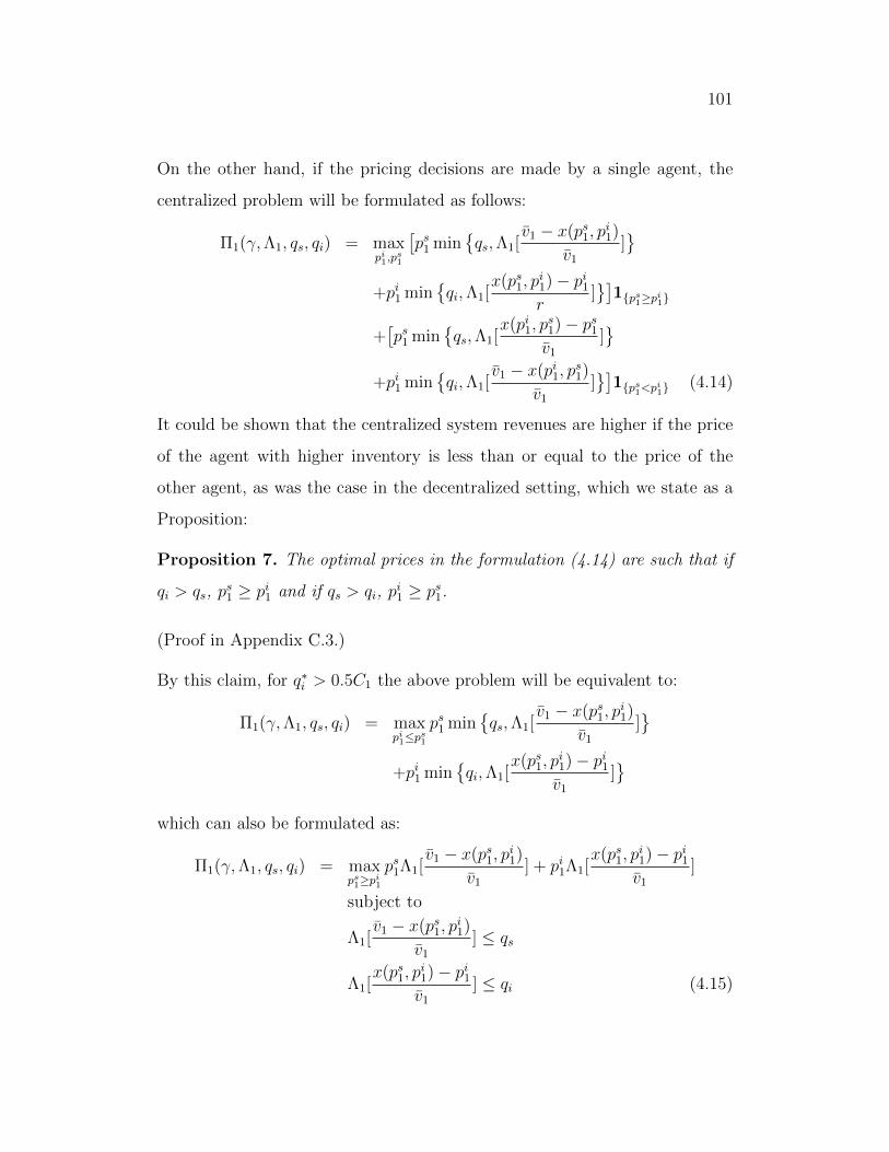
101
On the other hand, if the pricing decisions are made by a single agent, the
centralized problem will be formulated as follows:
Π1(γ,Λ1, qs, qi) = maxpi1,p
s1
[ps1 min
{qs,Λ1[
v1 − x(ps1, pi1)
v1
]}
+pi1 min{qi,Λ1[
x(ps1, pi1)− pi1r
]}]
1{ps1≥pi1}
+[ps1 min
{qs,Λ1[
x(pi1, ps1)− ps1v1
]}
+pi1 min{qi,Λ1[
v1 − x(pi1, ps1)
v1
]}]
1{ps1<pi1} (4.14)
It could be shown that the centralized system revenues are higher if the price
of the agent with higher inventory is less than or equal to the price of the
other agent, as was the case in the decentralized setting, which we state as a
Proposition:
Proposition 7. The optimal prices in the formulation (4.14) are such that if
qi > qs, ps1 ≥ pi1 and if qs > qi, p
i1 ≥ ps1.
(Proof in Appendix C.3.)
By this claim, for q∗i > 0.5C1 the above problem will be equivalent to:
Π1(γ,Λ1, qs, qi) = maxpi1≤ps1
ps1 min{qs,Λ1[
v1 − x(ps1, pi1)
v1
]}
+pi1 min{qi,Λ1[
x(ps1, pi1)− pi1v1
]}
which can also be formulated as:
Π1(γ,Λ1, qs, qi) = maxps1≥pi1
ps1Λ1[v1 − x(ps1, p
i1)
v1
] + pi1Λ1[x(ps1, p
i1)− pi1v1
]
subject to
Λ1[v1 − x(ps1, p
i1)
v1
] ≤ qs
Λ1[x(ps1, p
i1)− pi1v1
] ≤ qi (4.15)
102
The above formulation is concave in both ps1 and pi1. Call the prices that are
the maximizers of the above problem as the centralized prices pi∗1 (c) and ps∗1 (c).
Via the characterization of KKT conditions, these prices can be shown to take
the following optimal values under different cases:
(ps∗1 (c), pi∗1 (c))
=
(1323v1,
1123v1), if qs ≥ Λ1
323, qi ≥ Λ1
923
(23v1 − 7qsv1
9Λ1, v1
2− qsv1
6Λ1), if qs < Λ1
323, qi ≥ Λ1
12− 5
6qs
( v1
2+ qiv1
6Λ1, 5
8v1 − 3qiv1
8Λ1), if qs ≥ Λ1
38− 5
8qi, qi < Λ1
923
(v1 − 2(2qs+qi)v1
3Λ1, v1 − (qi+qs)v1
Λ1), otherwise
(4.16)
And the revenue in each case is stated as:
Π1(γ,Λ1, qs, qi) =
6Λ1
23v1, if qs ≥ 3Λ1
23, qi ≥ 9Λ1
23
16v1qs − 23
36(qs)2v1
Λ1+ Λ1
4v1, if qs <
3Λ1
23, qi ≥ Λ1
2− 5
6qs
38v1qi − 23
48v1(qi)
2
Λ1+ 3Λ1
16v1, if qs ≥ 3Λ1
8− 5
8qi, qi <
9Λ1
23
qs(v1 − 2(2qs+qi)v1
3Λ1) + qi(v1 − (qi+qs)v1
Λ1), otherwise
(4.17)
Again, to help visualize various cases of the problem for q∗i ≥ 0.5C1, please
refer to the Figure 4.3.
4.4 The Price of Anarchy
In this section, we will compare the profits of the decentralized system versus
the centralized system under various cases with respect to the relationship
between the market size and the inventories of the two agents.
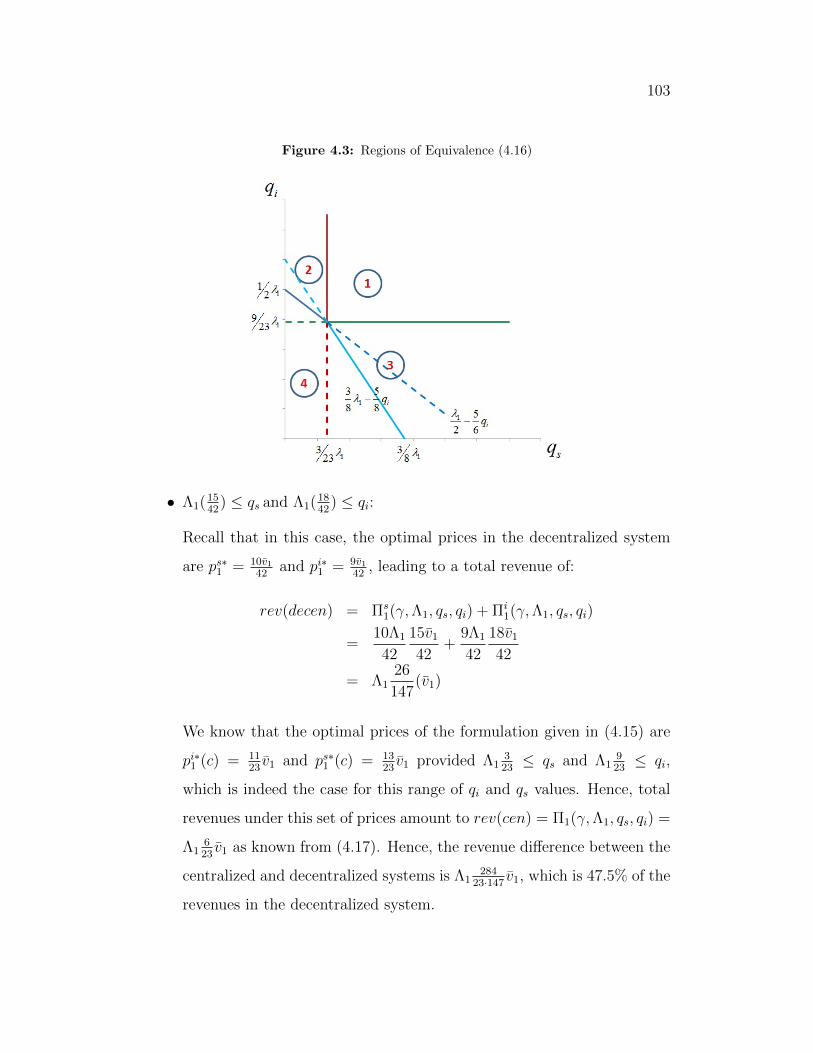
103
Figure 4.3: Regions of Equivalence (4.16)
• Λ1(1542
) ≤ qs and Λ1(1842
) ≤ qi:
Recall that in this case, the optimal prices in the decentralized system
are ps∗1 = 10v1
42and pi∗1 = 9v1
42, leading to a total revenue of:
rev(decen) = Πs1(γ,Λ1, qs, qi) + Πi
1(γ,Λ1, qs, qi)
=10Λ1
42
15v1
42+
9Λ1
42
18v1
42
= Λ126
147(v1)
We know that the optimal prices of the formulation given in (4.15) are
pi∗1 (c) = 1123v1 and ps∗1 (c) = 13
23v1 provided Λ1
323≤ qs and Λ1
923≤ qi,
which is indeed the case for this range of qi and qs values. Hence, total
revenues under this set of prices amount to rev(cen) = Π1(γ,Λ1, qs, qi) =
Λ1623v1 as known from (4.17). Hence, the revenue difference between the
centralized and decentralized systems is Λ1284
23·147v1, which is 47.5% of the
revenues in the decentralized system.
104
• 15Λ1
42> qs and 2
3Λ1 − 2qs
3≤ qi:
Recall that in this case, the decentralized system optimal prices are ps∗1 =
5v1
9− 8qsv1
9Λ1and pi∗1 = v1
3− qsv1
3Λ1, leading to a total revenue of:
rev(decen) = Πs1(γ,Λ1, qs, qi) + Πi
1(γ,Λ1, qs, qi)
= (5v1
9− 8qsv1
9Λ1
)qs +Λ1
v1
(v1
3− qsv1
3Λ1
)(2v1
3− 2qsv1
3Λ1
)
=1
9v1qs −
6
9
(qs)2v1
Λ1
+ Λ12
9v1
In this case, based on the values of qi and qs, two subcases can be ob-
served:
– 15Λ1
42> qs ≥ Λ1
323
: The maximizer prices of the unconstrained rev-
enue function, namely pi∗1 (c) = 1123v1 and ps∗1 (c) = 13
23v1, produce a
sales quantity Λ1323
for the seller; hence these prices are again op-
timal, leading to a total system revenue of rev(cen) = Λ1623v1. It
could be shown that:
rev(cen)− rev(decen) = Λ16
23v1 − (
1
9v1qs −
6
9
(qs)2v1
Λ1
+ Λ12
9v1)
= Λ18
23 · 9v1 −
1
9v1qs +
6
9
(qs)2v1
Λ1
≥ 0
for 15Λ1
42> qs ≥ Λ1
323
. Furthermore, the ratio of additional revenue
to be captured by centralized price decisions to the total revenue of
the decentralized system is:
rev(cen)− rev(decen)
rev(decen)=
Λ18
23·9 v1 − 19v1qs + 6
9(qs)2v1
Λ1
19v1qs − 6
9(qs)2v1
Λ1+ Λ1
29v1
105
which can be shown to increase in qs; hence attains its minimum
value at qs = Λ1323
which is 15.8%; and its maximum value at
qs = Λ11542
, which is 47.5%.
– qs < Λ1323
: In this case, as clear from (4.16), the formulation (4.15)
is maximized at pi∗1 (c) = v1
2− qsv1
6Λ1, leading to ps∗1 (c) = 2v1
3− 7qsv1
9Λ1
and a total revenue of rev(cen) = 16v1qs − 23
36(qs)2v1
Λ1+ Λ1
14v1. The
difference between the two revenue figures is therefore:
rev(cen)− rev(decen) =1
18v1qs +
1
36
(qs)2v1
Λ1
+ Λ11
36v1
which is clearly positive, and increasing in v1 and qs. Furthermore,
the ratio of additional revenue to be captured by centralized price
decisions to the total revenue of the decentralized system is:
rev(cen)− rev(decen)
rev(decen)=
118v1qs + 1
36(qs)2v1
Λ1+ Λ1
136v1
19v1qs − 6
9(qs)2v1
Λ1+ Λ1
29v1
which can be shown to increase in qs, and attains a value between
12.5% and 47.5%.
• Λ1(12− qi
3Λ1) ≤ qs and Λ1(18
42) > qi:
Recall that in this case, the decentralized system prices are ps∗1 = v1
3−
2qiv1
9Λ1and pi∗1 = v1
2− 2qiv1
3Λ1leading to a total revenue of:
rev(decen) = Πs1(γ,Λ1, qs, qi) + Πi
1(γ,Λ1, qs, qi)
= Λ13
2(1
3− 2qi
9Λ1
)2 + (v1
2− 2qiv1
3Λ1
)qi
=5
18v1qi −
16
27
v1(qi)2
Λ1
+ Λ11
6v1
Regarding the centralized system, again there are two subcases:
106
– 1842
Λ1 > qi ≥ 923
Λ1: The maximizer prices of the unconstrained
revenue function, namely pi∗1 (c) = 1123v1 and ps∗1 (c) = 13
23v1, produce
a sales quantity 923
Λ1 for the investors; hence these prices are again
optimal, leading to a total system revenue of rev(cen) = Λ1623v1.
Then the ratio of additional revenue to be captured by centralized
price decisions to the total revenue of the decentralized system is:
rev(cen)− rev(decen)
rev(decen)=
Λ113
23·6 v1 − 518v1qi + 16
27(qi)
2v1
Λ1
518v1qi − 16
27(qi)2v1
Λ1+ Λ1
16v1
which can be shown to increase in qi; hence attains its minimum
value at qi = Λ1923
which is 41.2%; and its maximum value at
qi = Λ11842
, which is 47.5%.
– qi <923
Λ1: In this case, as clear from (4.16), the formulation (4.15)
is maximized at ps∗1 (c) = v1
2+ qiv1
6Λ1and pi∗1 (c) = 5v1
8− 3qiv1
8Λ1; and leads
to a total system revenue of rev(cen) = 38v1qi − 23
48v1(qi)
2
Λ1+ Λ1
316v1.
Then the ratio of additional revenue to be captured by centralized
price decisions to the total revenue of the decentralized system is:
rev(cen)− rev(decen)
rev(decen)=
772v1qi + 49
27·16v1(qi)
2
Λ1+ Λ1
148v1
518v1qi − 16
27v1(qi)2
Λ1+ Λ1
16v1
which can be shown to increase in qi; hence attains its minimum
value at qi = 0 which is 12.5%; and its maximum value at qi = Λ1923
,
which is 41.2%.
• Λ11542> qs and Λ1(2
3)− 2
3qs > qi OR Λ1(18
42) > qi and Λ1(1
2)− 1
3qi > qs:
Recall that in this case, ps∗1 = v1 − 2(2qs+qi)v1
3Λ1and pi∗1 = v1 − (qi+qs)v1
Λ1
107
leading to a total revenue of:
rev(decen) = Πs1(γ,Λ1, qs, qi) + Πi
1(γ,Λ1, qs, qi)
= qs(v1 −2(2qs + qi)v1
3Λ1
) + (v1 −(qi + qs)v1
Λ1
)qi
= v1qi + v1qs −5
3
v1qsqiΛ1
− 4
3
v1(qs)2
Λ1
− v1(qi)2
Λ1
As before, there are different cases to consider in the centralized system:
– qi ≥ 923
Λ1 and qs ≥ Λ1323
: In this case, the maximizer prices of the
unconstrained revenue function, namely pi∗1 (c) = 1123v1 and ps∗1 (c) =
1323v1 are optimal for the centralized system, and the system revenue
is equivalent to rev(cen) = Λ1623v1. It could be shown that the ratio
rev(cen)−rev(decen)rev(decen)
could be as high as 47.5% in this range of (qi, qs)
values.
– qs < Λ1323
and qi ≥ Λ1923
: In this case, the formulation (4.15) is
maximized at pi∗1 (c) = v1
2− qsv1
6Λ1and ps∗1 (c) = 2v1
3− 7qsv1
9Λ1, leading
to rev(cen) = 16v1qs − 23
36(qs)2v1
Λ1+ Λ1
14v1. It could be shown that
rev(cen) > rev(decen) for this range of (qi, qs) values.
– qs ≥ Λ1323
and qi < Λ1923
: In this case, the formulation (4.15) is
maximized at ps∗1 (c) = v1
2+ qiv1
6Λ1and pi∗1 (c) = 5v1
8− 3qiv1
8Λ1; leading
to rev(cen) = 38v1qi − 23
48v1(qi)
2
Λ1+ Λ1
316v1. It could be shown that
rev(cen) > rev(decen) for this range of (qi, qs) values.
– qs < Λ1323
and qi < Λ1923
: In this case the optimal central prices are
equivalent to the optimal prices of the decentralized system. Hence,
the revenues in both cases are equivalent.
The case where q∗i ≤ 0.5C1 is symmetrical, so we skip the analysis.
108
In conclusion, the additional profit opportunities arising from centralized de-
cision making lies between 0% to 47.5% depending on the realization of Λ1.
4.5 Numerical Analysis: Evaluating a
Candidate Contracting Scheme
As clear from the analysis in the previous section, it is possible to increase the
revenues of both agents considerably by centralizing the pricing decisions. At
this point, various contracting schemes can be proposed to ensure cooperation
between the two agents. We will proceed with the following scheme, which
combines the spirit of “callable products” of the revenue management and the
“revenue sharing contracts” of the supply chain literature.
In this scheme, the seller offers the so-called “callable units” at t = 0 at a
price pc0 (≤ ps0) together with the regular units which are sold at ps0. However,
the inferior callable products come with a call option for the seller: If the
extra profit attained by centralizing the pricing decisions surpasses a certain
percentage or a certain amount (say, K1), the seller exercises her call option at
t = 1 by paying a percentage K0 on the top of their purchase price (or, again
a fixed option price per unit) to the investors, and gains the right to recall
and reprice the units of the investors. Thus, at t = 1, rather than having
to compete with the investors, the seller can price the units according to the
centralized system optimal (We still assume that the investor units and the
seller units should be priced differently. The reasoning for this practice could
be the fact that during the time period the investors owned the units, they
made structural changes inside these units that lead them to be perceived as
109
different than seller-owned units).
Provided that the expected profit of the investors under the contracting scheme
is higher than their expected profits in the previous system, the risk-neutral
investors would agree to this scheme. Or, it is possible to act cautiously, and
design a pricing scheme that leaves the investors with an equivalent or higher
revenue at each realization of the unknown random variables.
Let A denote the subset of the state space of Λ1 values that lead to a recall
and let A′ denote the contingencies that do not lead to a recall at t = 1. That
is:
Λ1 ∈ A⇒ Π1(γ,Λ1, qs, qi) ≥ (1 +K1)[Πs
1(γ,Λ1, qs, qi) + Πi1(γ,Λ1, qs, qi)
]Λ1 ∈ A′ ⇒ Π1(γ,Λ1, qs, qi) < (1 +K1)
[Πs
1(γ,Λ1, qs, qi) + Πi1(γ,Λ1, qs, qi)
]
where Π1(·) is the centralized system expected profits and Πs1(·) and Πi
1(·) are
the expected profits of the seller and the investors in the decentralized system
respectively.
Also, let Di,new0 (K0, K1, p
c0, p
s,new0 ) denote the callable units purchased by the
investors under the scheme (K0, K1, pc0, p
s,new0 ) where ps,new0 is the new price for
regular units at t = 0. Moreover, let qi,c(γ,Di,new0 , C1, p
c0) denote the units to
be claimed at t = 0.5. Then, the pricing scheme (K0, K1, pc0, p
s,new0 ) produces
the following expected profit functions for the seller 4:
4We denote the seller profit functions under the contracting scheme (K0,K1, pc0, p
s,new0 )
by adding a superscript “new”.
110
Πs,new1 (γ,Λ1, qs, qi,c) =
Π1(γ,Λ1, qs, qi,c)− (1 +K0)dpc0 × qi,c, if Λ1 ∈ A
Πs1(γ,Λ1, qs, qi,c), if Λ1 ∈ A′
Πs,new0 (C,Λ0, K0, p
c0) = max
ps,new0
[ps,new0
Λ0(v0 − ps,new0 )
v0
+ dpc0Di,new0
+Eγ,Λ1 [Πs,new1 (γ,Λ1, C1(ps,new0 )− qi,c, qi,c))]
]]
and the following profit functions for the investors:
Πi,new1 (γ,Λ1, qs, qi,c) =
(1 +K0)dpc0 × qi,c, if Λ1 ∈ A
Πi1(γ,Λ1, qs, qi,c), if Λ1 ∈ A′
Πi,new0.5 (γ,Di,new
0 , C1, pc0) = max
qi,c≤Di,new0
∫Λ1
Πi,new1 (γ,Λ1, C1 − qi,c, qi,c)f(Λ1)dΛ1
−(1− d)pc0qi,c
Πi,new0 (pc0, p
s,new0 ) = max
Di,new0
[Eγ[Π
i,new0.5 (γ,Di,new
0 , C1, pc0)]− dpc0D
i,new0
]
Clearly, for the seller to offer and the investors to accept the contracting
scheme, the following inequalities must hold:
Πs,new0 (C,Λ0, K0, K1, p
c0) ≥ Πs
0(C,Λ0)
Πi,new0 (pc0, p
s,new0 ) ≥ Πi
0(ps,new0 )
The only problem with the above situation could be the fact that offering
callable units might also be appealing to the regular buyers who initially had no
intention of making profit from buying and reselling the units. But in practice,
111
regular buyers are prone to incurring additional costs during the process of
reselling the units. This phenomenon stems from several reasons. For instance,
unlike investors, regular individuals who would like to sell their houses do not
have efficient channels to sell the units; hence this arbitrage opportunity does
not come as naturally in their part as it does for the investors. Thus, by
setting the fixed premium K0 such that their total revenue per recalled unit
minus their transaction costs is negative, it is possible to render the process
of investing in the callable units non-profitable for regular buyers.
In practice, it is difficult to compute the K0, K1 and pc0 values optimally,
and the nature of the contract changes based on how the developer and the
investor agree to split the profits. Therefore, rather than attempting to find
the optimal values based on some assumptions on sharing the profit, we will
evaluate the performances of various contracting schemes with for a number
of (K0, K1, pc0) triplets.
Numerical Example: Consider the problem of a developer who wants to
sell C = 100 units. The market size at t = 0 is Λ0=50, while it can take
values Λ1=50, 100 or 150 with equal probabilities at t = 1. Assume that the
willingness to pay values of the regular buyers at t = 0 is uniformly distributed
in the range [0, $200, 000], and the upper bound of valuations vary uniformly
between $100,000 and $300,000 at t = 1 (i.e., γ ∼ U[−$100, 000, $100, 000]).
Under the above setting, the optimal price of the seller at t = 0 turns out to be
ps∗0 = $72, 000. The investors then make a deposit for only Di0(ps0) = 15 units.
The expected seller and investor profits then take the values Πs0 = $6.648M
and Πi0 = $330K.
On the other hand, various contracting schemes (K0, K1, pc0, p
s,new0 ) produce
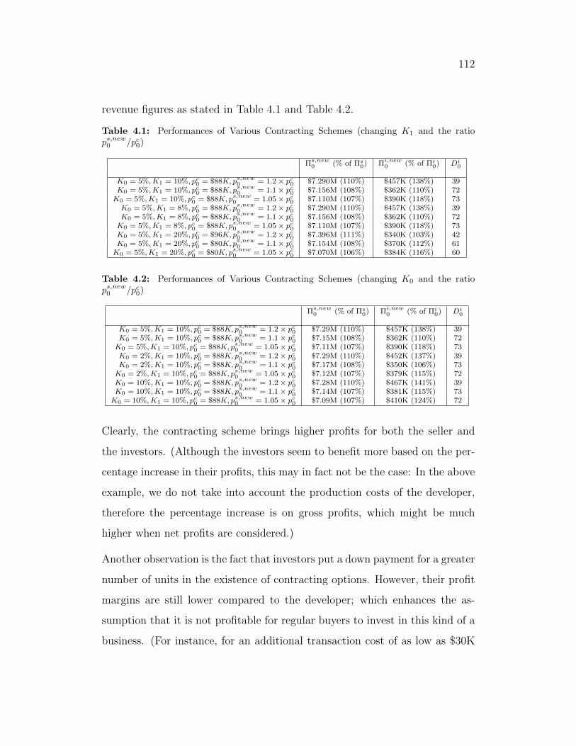
112
revenue figures as stated in Table 4.1 and Table 4.2.
Table 4.1: Performances of Various Contracting Schemes (changing K1 and the ratiops,new0 /pc0)
Πs,new0 (% of Πs
0) Πi,new0 (% of Πi
0) Di0
K0 = 5%,K1 = 10%, pc0 = $88K, ps,new0 = 1.2× pc0 $7.290M (110%) $457K (138%) 39
K0 = 5%,K1 = 10%, pc0 = $88K, ps,new0 = 1.1× pc0 $7.156M (108%) $362K (110%) 72
K0 = 5%,K1 = 10%, pc0 = $88K, ps,new0 = 1.05× pc0 $7.110M (107%) $390K (118%) 73
K0 = 5%,K1 = 8%, pc0 = $88K, ps,new0 = 1.2× pc0 $7.290M (110%) $457K (138%) 39
K0 = 5%,K1 = 8%, pc0 = $88K, ps,new0 = 1.1× pc0 $7.156M (108%) $362K (110%) 72
K0 = 5%,K1 = 8%, pc0 = $88K, ps,new0 = 1.05× pc0 $7.110M (107%) $390K (118%) 73
K0 = 5%,K1 = 20%, pc0 = $96K, ps,new0 = 1.2× pc0 $7.396M (111%) $340K (103%) 42
K0 = 5%,K1 = 20%, pc0 = $80K, ps,new0 = 1.1× pc0 $7.154M (108%) $370K (112%) 61
K0 = 5%,K1 = 20%, pc0 = $80K, ps,new0 = 1.05× pc0 $7.070M (106%) $384K (116%) 60
Table 4.2: Performances of Various Contracting Schemes (changing K0 and the ratiops,new0 /pc0)
Πs,new0 (% of Πs
0) Πi,new0 (% of Πi
0) Di0
K0 = 5%,K1 = 10%, pc0 = $88K, ps,new0 = 1.2× pc0 $7.29M (110%) $457K (138%) 39
K0 = 5%,K1 = 10%, pc0 = $88K, ps,new0 = 1.1× pc0 $7.15M (108%) $362K (110%) 72
K0 = 5%,K1 = 10%, pc0 = $88K, ps,new0 = 1.05× pc0 $7.11M (107%) $390K (118%) 73
K0 = 2%,K1 = 10%, pc0 = $88K, ps,new0 = 1.2× pc0 $7.29M (110%) $452K (137%) 39
K0 = 2%,K1 = 10%, pc0 = $88K, ps,new0 = 1.1× pc0 $7.17M (108%) $350K (106%) 73
K0 = 2%,K1 = 10%, pc0 = $88K, ps,new0 = 1.05× pc0 $7.12M (107%) $379K (115%) 72
K0 = 10%,K1 = 10%, pc0 = $88K, ps,new0 = 1.2× pc0 $7.28M (110%) $467K (141%) 39
K0 = 10%,K1 = 10%, pc0 = $88K, ps,new0 = 1.1× pc0 $7.14M (107%) $381K (115%) 73
K0 = 10%,K1 = 10%, pc0 = $88K, ps,new0 = 1.05× pc0 $7.09M (107%) $410K (124%) 72
Clearly, the contracting scheme brings higher profits for both the seller and
the investors. (Although the investors seem to benefit more based on the per-
centage increase in their profits, this may in fact not be the case: In the above
example, we do not take into account the production costs of the developer,
therefore the percentage increase is on gross profits, which might be much
higher when net profits are considered.)
Another observation is the fact that investors put a down payment for a greater
number of units in the existence of contracting options. However, their profit
margins are still lower compared to the developer; which enhances the as-
sumption that it is not profitable for regular buyers to invest in this kind of a
business. (For instance, for an additional transaction cost of as low as $30K
113
per unit on the top of investor costs, it is not profitable for the regular buyers
to invest in the regular units.)
Also observe that the price of the contracting option and the price of the
regular units both increase in the presence of the contracting scheme. That is
mainly because, due to the existence of higher profit opportunities at t = 1 by
a more efficient management, the developer prefers to keep a greater number of
units to be sold in the later period. This phenomenon may also help increase
the market value of the units.
Finally, the effect of varying K0 or K1 is not huge on the profits of the two
parties at least within the above set of values.
As a side note we would like to emphasize that the above contracting schemes
are only some selections among the set of feasible contracts. For instance,
for the base case, it is possible to select another contracting scheme with
(K0, K1, pc0, p
s,new0 ) = (5%, 10%, $84K, $92K) which brings the expected rev-
enues of Πs1 = $7.017M to the seller and Πi
1 = $481K to the investors. That is,
by modulating the contracting price, it is possible to shift the additional prof-
its to either side, which might itself be a negotiation tool among the developer
and the investors in the design of the contract.
Keeping the contracting scheme variables fixed at K0 = 5%, K1 = 10%, and
ps,new0 = 1.1 × pc0, the selection of the best contracting price and the effect
of the problem parameters on the profits of both systems (with or without
contract) are analyzed in Table 4.3.
The results in the above table suggest the following insights: Contracting
schemes are especially helpful in highly uncertain environments (e.g. γ ∼
U[−200K, 200K]); and in the cases where buyer valuations are lower (e.g.
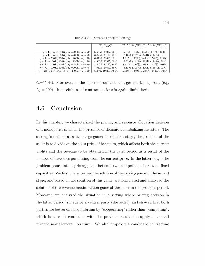
114
Table 4.3: Different Problem Settings
Πs0,Π
i0, p
s∗0 Πs,new
0 (%ofΠs0),Πi,new
0 (%ofΠi0), pc∗0
γ ∼ U[−50K, 50K], v0=200K, Λ0=50 6.65M, 330K, 72K 7.16M (108%) 362K (110%), 88Kγ ∼ U[−50K, 50K], v0=200K, Λ0=50 6.82M, 301K, 72K 7.15M (105%), 344K (114%), 88K
γ ∼ U[−200K, 200K], v0=200K, Λ0=50 6.41M, 288K, 88K 7.21M (112%), 444K (154%), 112Kγ ∼ U[−100K, 100K], v0=150K, Λ0=50 4.83M, 203K, 60K 5.53M (114%), 281K (124%), 76Kγ ∼ U[−100K, 100K], v0=250K, Λ0=50 8.44M, 421K, 88K 8.91M (106%), 491K (117%), 108Kγ ∼ U[−100K, 100K], v0=200K, Λ0=75 7.91M, 246K, 88K 8.12M (103%), 409K (166%), 92Kγ ∼ U[−100K, 100K], v0=200K, Λ0=100 8.99M, 197K, 100K 9.03M (100.9%), 284K (144%), 104K
v0=150K). Moreover, if the seller encounters a larger market upfront (e.g.
Λ0 = 100), the usefulness of contract options is again diminished.
4.6 Conclusion
In this chapter, we characterized the pricing and resource allocation decision
of a monopolist seller in the presence of demand-cannibalizing investors. The
setting is defined as a two-stage game: In the first stage, the problem of the
seller is to decide on the sales price of her units, which affects both the current
profits and the revenue to be obtained in the later period as a result of the
number of investors purchasing from the current price. In the latter stage, the
problem pours into a pricing game between two competing sellers with fixed
capacities. We first characterized the solution of the pricing game in the second
stage, and based on the solution of this game, we formulated and analyzed the
solution of the revenue maximization game of the seller in the previous period.
Moreover, we analyzed the situation in a setting where pricing decision in
the latter period is made by a central party (the seller), and showed that both
parties are better off in equilibrium by “cooperating” rather than “competing”,
which is a result consistent with the previous results in supply chain and
revenue management literature. We also proposed a candidate contracting
115
scheme that helps coordinate the system and reach system optimal profits.
The analysis of this chapter promises a wide avenue for future research: For
instance, it is possible to suggest various other forms of coordinating contracts,
and their performances should be evaluated in different markets. As another
research avenue, the game could be carried to a multi-period setting: In that
case, the timing of sales and purchase decisions appears as an additional deci-
sion variable for the investors; and the seller needs to decide how many units
to offer at each instant in addition to setting the unit prices.
116
Bibliography
A. Ben-Tal, A. N., C. Roos. 2002. Robust solutions of uncertain quadratic andconic-quadratic problems. SIAM Journal on Optimization 13(2) 535–560.
A. Ben-Tal, E. G., A. Goryashko, A. Nemirovski. 2004. Adjustable robustsolutions of uncertain linear programs. Mathematical Programming 99(2)351376.
A. Ben-Tal, S. B., A. Nemirovski, 2005. Control of uncertainty-affected discretetime linear systems via convex programming.
Ball, M. O., M. Queyranne. 2009. Toward robust revenue management: Com-petitive analysis of online booking. Operations Research 57(4) 950–963.
Bansal, M., C. Maglaras. 2009. Dynamic pricing when customers strategicallytime their purchase: asymptotic optimality of a two price policy. Journal ofRevenue and Pricing Management 8 42–66.
Ben-Tal, A., A. Nemirovski. 1998. Robust convex optimization 23(4) 769–805.
Bergemann, D., K. Schlag. 2008. Pricing without priors. Journal of theEuropean Economic Association 6(2-3) 560–569.
Bernstein, F., F. Chen, A. Federgruen, 2002. Coordinating supply chains withsimple pricing schemes: The role of vendor managed inventories.
Bernstein, F., A. Federgruen. 2003. Pricing and replenishment strategies ina distribution system with competing retailers. Operations Research 51(3)409–426.
Bernstein, F., A. Federgruen. 2005. Decentralized supply chains with compet-ing retailers under demand uncertainty. Management Science 51(1) 18–29.

117
Bertsimas, D., D. B. Brown. 2007. Constrained stochastic lqc: A tractableapproach. IEEE Transactions on Automatic Control 52(10) 18261841.
Bertsimas, D., M. Sim. 2003. The price of robustness 52 35–53.
Bertsimas, D., A. Thiele. 2004. A robust optimization approach to supplychain manage- ment. Proceedings of the 14th IPCO 86–100.
Besbes, O., C. Maglaras, 2009. Dynamic pricing with financial milestones:Feedback-form policies. Working Paper.
Bhandari, A., N. Secomandi, 2009. Comparison of negotiation mechanisms inrevenue management. Working Paper.
Birge, J. R., J. Drogosz, I. Duenyas. 1998. Setting single-period optimalcapacity levels and prices for substitutable products. The InternationalJournal of Flexible Manufacturing Systems 10 407430.
Brumelle, S., J. McGill. 1993. Airline seat allocation with multiple nested fareclasses 41(1) 127–137.
Cachon, G. P., 2003. Supply chain coordination with contracts.
Carr, S., I. Duenyas. 2000. Optimal admission control and sequencing ina make-to-stock/ make-to-order production system. Operations Research48(5) 709–720.
Carr, S., W. Lovejoy. 2000. The inverse newsvendor problem: Choosingan optimal portfolio for capacitated resources. Management Science 46(7)912–927.
Chatterjee, K., W. Samuelson. 1983. Bargaining under incomplete informa-tion. Operations Research 31(5) 835–861.
Clifford, S., 2012. The ny times article in the adresshttp://www.nytimes.com/2012/03/28/business/retailers-rush-to-adjust-to-price-smart-shoppers.html.
D. Bertsimas, D. A. I., P. A. Parrilo. 2010. Optimality of affine policies inmulti-stage robust optimization. Mathematics of Operations Research 35363–394.
Dantzig, G. B. 1969. A hospital admission problem. Technical Report. Oper-ations Research House, Stanford University, Stanford, California .
118
Deneckere, R., J. Peck. 1995. Competition over price and service rate whendemand is stochastic: a strategic analysis. Journal of Economics 26(1)148–162.
Ding, Q., P. Kouvelis., J. Milner. 2006. Dynamic pricing through customer dis-counts for optimizing multi-class customers demand fulfillment. OperationsResearch 54(1) 169–183.
Duenyas, I. 2000. Single facility due date setting with multiple customerclasses. Operations Research 48(5) 709–720.
Duran, S., T. Liu, D. Simchi-Levi, J. Swann. 2008. Policies utilizing tacticalinventory for service-differentiated customers. Operations Research Letters36(2) 259–264.
El Ghaoui, L., H. Lebret. 1997. Robust solutions to least-squares problemswith uncertain data. 18(4) 1035–1064.
Eren, S., C. Maglaras. 2010. Monopoly pricing with limited demand informa-tion. Journal of revenue and pricing management 9(1-2) 23–48.
Eren, S., G. van Ryzin. 2006. Product line positioning without marked infor-mation. Working Paper, Columbia University, New York, NY 10027 .
Esogbue, O., A. Singh. 1976. A stochastic model for an optimal prioritybed distribution problem in a hospital ward. Operations Research 24(5)884–898.
Gallego, G., S. Kou. 2008. Revenue management of callable products. Man-agement Science 54(3) 550–564.
Gallego, G., O. Sahin, 2006. Inter-temporal valuations, product design andrevenue management.
Gallego, G., G. van Ryzin. 1994. Optimal dynamic pricing of inventories withstochastic demand over finite horizons. Management Science 40 999–1020.
Gallien, J. 2006. Dynamic mechanism design for online commerce. OperationsResearch 54 291–310.
Garstka, S. J., R. J.-B.Wets. 1974. On decision rules in stochastic program-ming. Mathematical Programming 7(1) 117–143.
119
Gerchak, Y., D. Gupta, M. Henig. 1996. Reservation planning for electivesurgery under uncertain demand for emergency surgery. Management Sci-ence 42(3) 321–334.
Goldfarb, D., G. Iyengar. 2003. Robust convex quadratically constrainedprograms. Mathematical Programming 97(3) 495–515.
Grant, M., S. Boyd. 2008. CVX: MATLAB Software for Disciplined Convexprogramming.
Green, L. V., S. Savin, B. Wang. 2006. Managing patient service in a diagnosticmedical facility. Operations Research 54(1) 11–25.
Gupta, D., L. Wang, 2006. Manufacturing capacity revenue management.Forthcoming in Operations Research.
Ha, A. Y. 1997a. Inventory rationing in a make-to-stock production systemwith several demand classes and lost sales. Management Science 43(8)1093–1103.
Ha, A. Y. 1997b. Optimal dynamic scheduling policy for a make-to-stockproduction system. Operations Research 45(1) 42–53.
Harper, R., A. Shahani. 2002. Modeling for the planning and managementof bed capacities in hospitals. Journal of the Operational Research Society53(1) 11–18.
Harsanyi, J. C. 1956. Approaches to the bargaining problem before and afterthe theory of games. Econometrica 24(2) 144–157.
Herk, L. 1993. Consumer choice and cournot behavior in capacityconstrainedduopoly competition. Journal of Economics 24(3) 399–417.
Huang, X. 1995. A planning model for requirement of emergency beds. IMAJournal of Mathematics Applied in Medicine & Biology 12(3-4) 345–353.
Kerrigan, E., J. Maciejowski. 2004. Properties of a new parameterization forthe control of constrained systems with disturbances. Proceedings of the2004 American Control Conference 5(5) 46694674.
Kolesar, P. 1970. A markovian model for hospital admission scheduling.Management Science 16(6) 384–396.
120
Lan, Gao, M. Ball, I. Karaesmen. 2006. Revenue management with limiteddemand information. Working Paper, University of Maryland, College Park,MD .
Lee, T. C., M. Hersh. 1998. A model for dynamicairline seat inventory controlwith multiple seat bookings. Transportation Science 27(3) 252–265.
Lobel, G. Perakis, 2010. Network dynamic pricing through scenario basedoptimization. Working Paper.
Mackay, M. 2001. Practical experience with bed occupancy management andplanning systems: an australian view. Health Care Management Science4(1) 47–56.
Maglaras, C., J. Meissner. 2006. Dynamic pricing strategies for multi-productrevenue management problems 8(2) 136–148.
Maglaras, C., A. Zeevi. 2005. Pricing and design of differentiated services:Approximate analysis and structural insights. Operations Research 53(2)242–262.
McClean, S., P. Millard. 1995. A decision support system for bed-occupancymanagement and planning hospitals. IMA Journal of Mathematics Appliedin Medicine & Biology 12(3-4) 249–257.
Milsum, J., E. Turban, I. Vertinsky. 1973. Hospital admission systems: Theirevaluation and management. Management Science 19(6) 646–666.
Myerson, R. B. 1979. Incentive compatibility and the bargaining problem.Econometrica 47(1) 61–73.
Myerson, R. B. 1984. Two person bargaining problems with incomplete infor-mation. Econometrica 2(2) 461–487.
Myerson, R. B., M. A. Satterthwaite. 1983. Efficient mechanisms for bilateraltrading. Journal of Economic Theory 29 265–281.
Nash, J. C. 1950. The bargaining problem. Econometrica 18 151–162.
Patrick, J., M. L. Puterman. 2007. Improving resource utilization for diagnos-tic services through flexible inpatient scheduling: A method for improvingresource utilization. Journal of Operations Research Society 58(1) 235–245.
121
Perakis, G., G. Roels. 2007. Robust controls for network revenue management.Working Paper, UCLA, Los Angeles, CA 90095 .
Perakis, G., A. Sood. 2003. Competitive multi-period pricing with fixedinventories. Working Paper, MIT, Cambridge, MA, .
Porteus, E. L. 2002. Foundations of Stochastic Inventory Theory. StanfordUniversity Press.
Puu, T., I. Sushko. 2002. Oligopoly Dynamics. Springer.
Riley, J., R. Zeckhauser. 1983. Optimal selling strategies: When to haggle,when to hold firm. Quarterly Journal of Economics 98(2) 267–289.
Ruth, R. J. 1981. Mixed integer programming model for regional planning ofa hospital inpatient service. Management Science 27(5) 521–533.
Sinclair, J., 2009. The internet blog in the adress http://jsmineset.com/.
Smith-Daniels, V. L., S. B. Schweikhart, D. E. Smith-Daniels. 1988. Capacitymanagement in health care services: Review and future research directions.Decision Science 19(4) 889–919.
Sobel, M. J., R. Zhang. 2001. Inventory policies for systems with stochasticand deterministic demand. Operations Research 49(1) 157–162.
Su, X. 2007. Inter-temporal pricing with strategic customer behavior. Man-agement Science 53(3) 726–741.
Tang, Y., D. Xu, W. Zhou. 2007. Inventory rationing in a capacitated systemwith backorders and lost sales. Proceedings of the 2007 IEEE IEEM 1579–1583.
Tasnadi, A. 1999. A two-stage bertrand-edgeworth game. Economics Letters65 353–358.
Topkis, D. M. 1968. Optimal ordering and rationing policies in a nonstation-ary dynamic inventory model with n demand classes. Management Science15(3) 160–176.
Varma, G. D., N. Vettas. 2001. Optimal dynamic pricing with inventories.Economic Letters 72 335–340.
Vulcano, G., G. van Ryzin, C. Maglaras. 2002. Optimal dynamic auctions forrevenue management. Management Science 45(11) 1388–1407.
122
Young, J. P., 1962. A queuing theory approach to the control of hospitalinpatient census. Unpublished Doctoral Dissertation, The Johns HopkinsUniversity, IE dept.
Zhou, Y., X. Zhao. 2010. A two-demand-class inventory system with lost salesand backorders. Operations Research Letters 38(4) 261–266.
123
Appendix A
Appendix to Chapter 2
A.1 Proof of Theorem 1
First, define the following function based on (2.2):
Gt(st, xt) = L(st, xt) + α · EMt [ft+1((st + xt − C)+ +Mt)] .
Using an inductive argument, it can be shown that Gt(st, xt) is jointly concave
in its arguments for all t, and ft(st) is also concave and decreasing. The details
of this argument is standard and can be found in many of the papers mentioned
in the literature; in particular, we refer the reader to the proof of Lemma 4.3
and Theorem 4.2 in Porteus (2002).
Note the optimal decision x∗t (st) is obtained from maximizing a concave func-
tion Gt(st, xt) with respect to xt. From (2.3), it suffices to restrict the feasible
set of xt to [(C − st)+, C]. Then, from the definition of Gt above and the
124
definition of L(st, xt) in (2.1),
∂Gt(st, xt)
∂xt=
(r2 + w2)(1−H2t (xt))− w1 + α
∂EMt [ft+1((st + xt − C) +Mt)]
∂xt.
(A-1)
(i) Consider the right-hand-side of (A-1). Since ft+1 is concave, the partial
derivative in the last term is decreasing in st. It follows that ∂Gt(st, xt)/∂xt is
decreasing in st. Note also that the upper-bound of the feasible region C − stis decreasing in st. Therefore, we conclude that x∗t (st) is decreasing in st.
(ii) From (2.3) and its proof, it can be shown that Gt(st, xt) is increasing in xt
if xt ≤ (C−st)+. Thus, the optimal solution x∗t (st) must satisfy the first-order
condition that the partial derivative ∂Gt(st, xt)/∂xt at xt = x∗t (st) is zero.
Thus,
0 =∂Gt(st, xt)
∂xt
∣∣xt=x∗t (st)
= (r2 + w2)(1−H2t (x∗t (st)))− w1 +
α∂EMt [ft+1((st + xt − C) +Mt)]
∂xt
∣∣xt=x∗t (st)
.
Now, observe that
∂EMt [ft+1((st + xt − C) +Mt)]
∂xt
∣∣xt=x∗t (st)
=∂EMt [ft+1((st + ε+ xt − C) +Mt)]
∂xt
∣∣xt=x∗t (st)−ε
,
125
hence:
∂Gt(st + ε, xt)
∂xt
∣∣xt=x∗t (st)−ε
= (r2 + w2)(1−H2t (x∗t (st)− ε))− w1
+α∂EMt [ft+1((st + ε+ xt − C) +Mt)]
∂xt
∣∣xt=x∗t (st)−ε
≥ 0 .
This result shows that Gt(st + ε, xt) is increasing with respect to xt when
xt = x∗t (st)− ε. Thus, we conclude that x∗t (st + ε) ≥ x∗t (st)− ε.
�
A.2 Proof for Section 2.4.1
We modify the Bellman equation introduced in (2.2) to include the capacity
of the current period t:
ft(st) = ECt
[max
0≤xt≤Ct
[L(st, xt, Ct) + α · EMt [ft+1((st + xt − Ct)+ +Mt)]
]],
where the single-period net-revenue function (2.1) is now modified to
L(st, xt, Ct) = r2E min{xt, Dt}+ r1E[Mt]− w1(st + xt − Ct)+
−w2E[Dt − xt]+ .
Similar to the proof of Theorem 1, we define the following function:
Gt(st, xt, Ct) = L(st, xt, Ct) + α · EMt,Ct [ft+1((st + xt − Ct)+ +Mt]
An inductive argument similar to the one used Theorem 1 can be used to
show that each ft is concave in st, and Gt is jointly concave in (st, xt) for any
126
fixed Ct, for all t. Thus, given the capacity value Ct and the state variable st,
there exists an optimal value of xt, denoted by x∗t (st, Ct), that maximizes the
function Gt(st, xt, Ct). As before, from (2.3), it suffices to restrict the feasible
set of xt to [(Ct − st)+,∞). Then, the above definition of Gt implies
∂Gt(xt, st, Ct)
∂xt= (r2+w2)(1−H2
t (xt))−w1+α∂EMt [ft+1((st + xt − Ct) +Mt)]
∂xt.
(A-2)
(i) Consider the right-hand-side of (A-2). Since ft+1 is a concave function,
the partial derivative in the last term is decreasing in st. It follows that
∂Gt(xt, st, Ct)/∂xt is decreasing in st. Note also that the lower-bound of the
feasible region (Ct − st)+ is decreasing in st. Therefore, we conclude that
x∗t (st, Ct) is decreasing in st for fixed Ct.
(ii) As in the proof of Theorem 1, x∗t (st, Ct) satisfies the first-order condition
that the partial derivative ∂Gt(xt, st, Ct)/∂xt at xt = x∗t (st, Ct) is zero. Thus,
0 =∂Gt(xt, st, Ct)
∂xt
∣∣xt=x∗t (st,Ct)
= (r2 + w2)(1−H2t (x∗t (st, Ct)))− w1
+α∂EMt [ft+1((st + xt − Ct) +Mt)]
∂xt
∣∣xt=x∗t (st,Ct)
(A-3)
Observe that
∂EMt [ft+1((st + xt − Ct) +Mt)]
∂xt
∣∣xt=x∗t (st,Ct)
=∂EMt [ft+1((st + ε+ xt − Ct) +Mt)]
∂xt
∣∣xt=x∗t (st,Ct)−ε
.
Thus, by comparing the partial derivative of Gt(xt, st + ε, Ct) with respect to
127
xt at x∗t (st, Ct)− ε to (A-3), we obtain that
∂Gt(xt, st + ε, Ct)
∂xt
∣∣xt=x∗t (st,Ct)−ε
= (r2 + w2)(1−H2t (x∗t (st, Ct)− ε))− w1
+α∂EMt [ft+1((st + ε+ xt − Ct) +Mt)]
∂xt
∣∣xt=x∗t (st,Ct)−ε
is nonnegative since H2t is a CDF, an increasing function. This result shows
that Gt(xt, st + ε, Ct) is increasing with respect to xt when xt = x∗t (st, Ct)− ε,
which implies that x∗t (st + ε, Ct) ≥ x∗t (st, Ct)− ε.
(iii) Next, we prove that 0 ≤ x∗t (st, Ct + ε)− x∗t (st, Ct) ≤ ε .
Since x∗t (st, Ct) satisfies the first-order condition,
0 =∂Gt(xt, st, Ct)
∂xt
∣∣xt=x∗t (st,Ct)
= (r2 + w2)(1−H2t (x∗t (st, Ct)))− w1
+ α∂EMt [ft+1(st + xt − Ct +Mt)]
∂xt
∣∣xt=x∗t (st,Ct)
.
As before, observe that:
∂EMt [ft+1((st + xt − Ct) +Mt)]
∂xt
∣∣xt=x∗t (st,Ct)
=∂EMt [ft+1((st + xt − Ct − ε) +Mt)]
∂xt
∣∣xt=x∗t (st,Ct)+ε
.
Moreover, 1−H2t (x∗t (st, Ct)) ≥ 1−H2
t (x∗t (st, Ct) + ε). Thus,
0 ≥ (r2 + w2)(1−H2t (x∗t (st, Ct) + ε))− w1
+α∂EMt [ft+1((st + xt − Ct − ε) +Mt)]
∂xt
∣∣xt=x∗t (st,Ct)+ε
=∂Gt(xt, st, Ct + ε)
∂xt
∣∣xt=x∗t (st,Ct)+ε
.
Hence, Gt(xt, st, Ct+ε) is decreasing with respect to xt when xt = x∗t (st, Ct)+ε,
128
which implies that x∗t (st, Ct + ε) ≤ x∗t (st, Ct) + ε. Moreover,
0 ≤ (r2 + w2)(1−H2t (x∗t (st, Ct)))− w1
+α∂EMt [ft+1((st + xt − Ct − ε)+ +Mt)]
∂xt
∣∣xt=x∗t (st,Ct)
=∂Gt(xt, st, Ct + ε)
∂xt
∣∣xt=x∗t (st,Ct)
,
where the inequality follows from the fact that ft+1 is a concave function,
which implies
∂EMt [ft+1((st + xt − Ct − ε)+ +Mt)]
∂xt
∣∣xt=x∗t (st,Ct)
≥ ∂EMt [ft+1((st + xt − Ct) +Mt)]
∂xt
∣∣xt=x∗t (st,Ct)
.
Thus, Gt(xt, st, Ct + ε) is increasing with respect to xt when xt = x∗t (st, Ct),
which completes our proof.
�
A.3 Proof for Section 2.4.2
As in the proof of Theorem 1, define the following function:
Gt(st, xt) = L(st, xt)
+ αEMt
[max
0≤at≤Mt
−r1(Mt − at) + ft+1((st + xt − C)+ + at)
].
(A-4)
As before, an inductive argument establishes that each Gt is jointly concave,
and that each ft is concave and decreasing.
We first address the structure of the optimal policy given in (2.7). Define
φt(ω) = r1ω + ft+1(ω) .
129
Note that φt is a concave function. Let the maximizer of φt be denoted by Rt.
Observe that the optimization problem in the definition of (A-4) is related to
maximizing φt; in particular, it is equivalent to
maxzt≤ut≤zt+Mt
φt(ut) where zt = (st + xt − C)+ .
By the concavity of φt and the convexity of the interval [zt, zt + Mt], it can
be verified that the optimal solution to this maximization problem is to set
ut = Rt if Rt is feasible; otherwise, we choose ut such that zt + ut is as close
to the target Rt as possible. This is the optimal policy given in (2.7).
Furthermore, the properties that x∗t (st) is decreasing in st and that x∗t (st+ε) ≥
x∗t (st)− ε, for any ε > 0, follows directly from (2.7).
�
A.4 Proof for Section 2.4.3
It is convenient to define a mapping between the state vector st and st =
(s1t , . . . , s
nt ), where we define sit = s1
t + s2t + · · · + sit. Thus, sit refers to the
sum of all backlogged patients in classes 1 through i. Then, ζ(st, C − xt) =
ζ(st, C − xt), where
ζ(st, C − xt) =([s1t − C + xt
]+,[s2t − C + xt
]+, . . . , [snt − C + xt]
+).
Let wi1 = wi1 − wi+11 where we let wn+1
1 = 0 for convenience. Define
L(st, xt) = r2 · E min{xt, Dt}+n∑i=1
ri1 · E[M it ]−
n∑i=1
wi1 ·[sit − C + xt
]+−w2 · E[Dt − xt]+ .
130
Then, the dynamic programming formulation can be written as
f t(st) = max0≤xt≤C
Gt(st, xt) , where
Gt(st, xt) = L(st, xt) + α · EMt [f t+1(ζ(st, C − xt) + Mt)] .
For the terminal value, we let fT+1(sT+1) =∑n
i=1 vi ·(siT+1−si−1
T+1) =∑n
i=1(vi−
vi+1)·siT+1, where vn+1 = 0. Recall that vi−vi+1 ≤ 0 for each i by assumption.
Note that L(st, xt) is a jointly concave function. Then, it can be shown using
induction that each Gt(st, xt) is jointly concave and each f t(st) is also concave
and decreasing.
Now, let x∗t (st) denote the value of xt maximizing Gt(st, xt) with respect to xt.
As before, it suffices to restrict the feasible set of xt to [(C − snt )+, C]. Then,
from the definition of Gt and the definition of L, we can obtain the partial
derivative of Gt(st, xt) with resect to xt everywhere except finite points. For
xt ∈ ((C − sit)+, (C − si−1t )+):
∂Gt(st, xt)
∂xt= (r2 + w2)(1−H2
t (xt))−n∑j=1
wj1 · 1[xt>C−sjt ]
+ α∂EMt [f t+1(ζ(st, C − xt) + Mt)]
∂xt. (A-5)
where 1 is the indicator function. (We remark that the second term in the
right-hand-side of (A-5) is simply wi1 + · · ·+wn1 = wi1 since xt is in the interval
((C− sit)+, (C− si−1t )+). We write this way so that it becomes more clear how
this expression depends on st.)
(i) Based on (A-5), it can be shown as before that ∂Gt(st, xt)/∂xt is decreasing
in s. (To be technically correct, we should consider one-sided partial deriva-
tives, but we use the term “derivative” for expositional simplicity.) To sketch
the argument for this assertion, observe that the first term in (A-5) is inde-
131
pendent of s, the second term is also decreasing in s, and finally, the third
term is also decreasing in s since we have
∂EMt [f t+1(ζ(st, C − xt) + Mt)]
∂xt=∂EMt [f t+1((st − C + xt)
+ + Mt)]
∂xt
=n∑j=1
∂EMt [f t+1((st − C + xt)+ + Mt)]
∂sjt· 1[xt>C−sjt ] (A-6)
where each partial derivative in the right-most expression is non-positive and
decreasing in sjt since f t+1 is concave and decreasing.
Thus, we conclude that x∗(st) is decreasing in st. In particular, for any ε > 0,
we have x∗(st) ≥ x∗ (st + ε · (ei + ei+1 + · · ·+ en)). Thus, we obtain x∗t (st) ≥
x∗t (st + ε · ei) for any ε > 0.
(ii) From the definition of ζ, it is easy to show that for any st, xt and ε > 0,
ζ(st + ε · (ei + · · ·+ en), C − (xt − ε)) ≤ ζ(st, C − xt) for any i .
Then, since the expression in (A-6) is decreasing in st, it follows that
∂EMt [f t+1(ζ(st + ε · (ei + · · ·+ en), C − xt) + Mt)]
∂xt
∣∣xt−ε
≥∂EMt [f t+1(ζ(st, C − xt) + Mt)]
∂xt
∣∣xt.
Also, since H2t is a CDF, it follows that
(1−H2t (xt − ε)) ≥ (1−H2
t (xt)) .
Finally,
i−1∑j=1
wj1 · 1[xt−ε>C−sjt ] +n∑j=i
wj1 · 1[xt−ε>C−sjt−ε]≤
n∑j=1
wj1 · 1[xt>C−sjt ]
132
Therefore, from (A-5), we obtain that, for any st and xt,
∂Gt(st + ε · (ei + · · ·+ en), xt)
∂xt
∣∣xt−ε
≥ ∂Gt(st, xt)
∂xt
∣∣xt.
Applying the above inequality to xt = x∗(st), we obtain
x∗(st + ε · (ei + ei+1 + · · ·+ en)
)≥ x∗(st)− ε.
Thus, x∗t (st + ε · ei) ≥ x∗t (st)− ε.
�
133
Appendix B
Appendix to Chapter 3
B.1 Proof of Theorem 3
First, note that any optimal strategy should satisfy b(vb) ≤ vb and s(vs) ≥
vs to be feasible; hence, this will be our implicit assumption throughout the
analysis. Also assume that the optimal strategies are nondecreasing in the
valuations of the bidders, which will also be shown to hold.
In the minimax absolute regret minimization problem (3.7) of the seller, the
innermost maximization takes the following values depending on the relation-
ship among b, s and vs:
maxs′
[(kb+ (1− k)s′ − vs)1{b≥s′} − (kb+ (1− k)s− vs)1{b≥s}]
=
0 if b < vs
(b− vs) if vs ≤ b ≤ s
(b− vs)− (kb+ (1− k)s− vs) if b > s
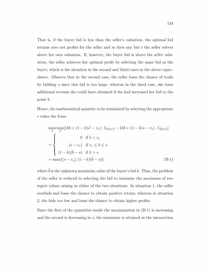
134
That is, if the buyer bid is less than the seller’s valuation, the optimal bid
returns zero net profits for the seller and so does any bid s the seller selects
above her own valuation. If, however, the buyer bid is above the seller valu-
ation, the seller achieves her optimal profit by selecting the same bid as the
buyer; which is the situation in the second and third cases in the above equiv-
alence. Observe that in the second case, the seller loses the chance of trade
by bidding s since this bid is too large; whereas in the third case, she loses
additional revenue she could have obtained if she had increased her bid to the
point b.
Hence, the mathematical quantity to be minimized by selecting the appropriate
s takes the form:
maxb
maxs′
[(kb+ (1− k)s′ − vs) · 1{b≥s′} − (kb+ (1− k)s− vs) · 1{b≥s}]
=
0 if b < vs
(s− vs) if vs ≤ b ≤ s
(1− k)(b− s) if b > s
= max{(s− vs), (1− k)(b− s)} (B-1)
where b is the unknown maximum value of the buyer’s bid b. Thus, the problem
of the seller is reduced to selecting the bid to minimize the maximum of two
regret values arising in either of the two situations: In situation 1, the seller
overbids and loses the chance to obtain positive return; whereas in situation
2, she bids too low and loses the chance to obtain higher profits.
Since the first of the quantities inside the maximization in (B-1) is increasing
and the second is decreasing in s, the minimizer is attained at the intersection
135
point, i.e:
s∗ARMC(vs) = argmins
max{(s− vs), (1− k)(b− s)}
⇒ s∗ARMC(vs)− vs = (1− k)(b− s∗ARMC(vs))
⇒ s∗ARMC(vs) =vs
2− k+
(1− k)
2− kb
Via a symmetrical analysis for the buyers, we obtain b∗ARMC(vb) = vb1+k
+ k1+k
¯s. Finally, since s∗ and b∗ should be best responses to each other and are
increasing in vs and vb respectively, we find that the functions s∗ARMC(vs) =
vs2−k + (1−k)vb
2+
k(1−k)¯vs
2(2−k)and b∗ARMC(vb) = vb
1+k+
k¯vs2
+ k(1−k)vb2(1+k)
are the solutions
of the above equations and they satisfy all previously made assumptions. Fur-
thermore, when the equations (3.1) and (3.2) are solved simultaneously for a
game where both valuations are distributed uniformly on the given ranges,
it is seen that the resulting equilibrium bidding functions are identical to the
functions given by (3.9) and (3.10).
�
B.2 Analysis of the One-to-one Negotiation
Problem between an Informed and
Uninformed Agent
Consider the one-to-one negotiation problem between a single seller and a
single buyer. We know the solution to this problem when (i) both the seller
and the buyer know each other’s distribution function, (ii) neither the seller
nor the buyer know each other’s distribution function, but they both know the
range of the opponent valuations and employ ARMC approach to decide their
136
bid. In this note, we will analyze a third option, i.e. (iii) the case where the
seller knows the buyer distribution function, Fb, while the buyer only knows
the range the seller’s valuation can come from, [¯vs, vs] (or, vice-versa).
During the analysis, we will implicitly assume that the equilibrium bidding
functions s(.) and b(.) are increasing in the seller and the buyer valuations
respectively. At the end of the analysis, we will indeed show that this claim is
true, provided that the following assumption holds:
Assumption: Fb is a distribution function with decreasing hazard rate (DFR).
The revenue maximization problem of the seller takes the form:
Πs(s, vs) = maxs∈[vs,b]
∫ b
s
(kb+ (1− k)s− vs)gb(b)db,
= maxs∈[vs,b(vb)]
∫ vb
b−1(s)
(kb(vb) + (1− k)s− vs)fb(vb)dvb,
which is maximized at the value s that satisfies the following equation:
(1− k)(1− Fb(b−1[s]))b′(b−1[s])− fb(b−1[s])(s− vs) = 0 (B-2)
At this point, the seller does not know the function b(.), or its derivative b′(.).
Thus, we turn our attention to the buyer’s problem, which takes the form:
argminb
{maxs
maxb′
[(vb − (kb′ + (1− k)s)) · 1{b′≥s}
−(vb − (kb+ (1− k)s)) · 1{b≥s}]}
= argminb
{max{(vb − b), k(b−
¯s)}}
(B-3)
given that the buyer employs ARMC approach, by the analysis in the proof
of Theorem 3.
137
Observe that, if the buyer is able to characterize the value of the lowest seller
bid,¯s = s(
¯vs), the solution of the equation (B-3) leads to the following bidding
function:
b(vb) =vb
k + 1+
k¯s
k + 1(B-4)
Hence, the seller’s problem is equivalent to finding the s value that satisfies:
(1− k)(1− Fb(s(k + 1)− k¯s))
1
k + 1− fb(s(k + 1)− k
¯s)(s− vs) = 0
by inserting the appropriate values of b and b′ into the equation (B-2).
Finally, the value of¯s is found from the equation:
(1− k)(1− Fb(¯s))
1
k + 1− fb(
¯s)(
¯s−
¯vs) = 0
which is then used to characterize the final form of the function b(.).
Moreover, both b(.) and s(.) become nondecreasing in the respective valuations
provided that Fb is a function with decreasing failure rate (which is a sufficient
condition, but not a necessary one for s(.) to be an increasing function). A
symmetrical problem can be solved for the case where the buyer knows the
seller distribution function, Fs, while the seller only knows the range buyer’s
valuation can come from, i.e. [¯vb, vb].
�
B.3 Proof of Theorem 6
As before, our implicit assumptions are that the optimal strategies satisfy b(vb)
≤ vb and s(vs) ≥ vs; and that the optimal strategies are nondecreasing in the
valuations of the bidders.
138
Since buyers are naive (i.e. they play a one-to-one game with the seller re-
gardless of the seller’s inventory or other buyers in the market), their problem
takes the form:
argminb{max
smaxb′
[(vb − (kb′ + (1− k)s)) · 1{b′≥s}
−(vb − (kb+ (1− k)s)) · 1{b≥s}]}
= max{(vb − b), k(b−¯s)}
as before. As they assume that the seller is also playing a one-to-one game with
them, they simply compute their optimal bidding strategy by solving the two
ARMC problems simultaneously, therefore reaching at the same equilibrium
bidding function as in the one-to-one game, i.e. b∗ARMC .
On the other hand, the seller’s problem is now different: Given that the bidding
function of the buyers is b∗ARMC , how should she select the bid st = s, ∀t, that
would minimize her maximum regret for all distribution functions Fb of buyers?
argmins{max
Fb
maxs′
[ ∫ T
t=0
Λt[
∫ vb
b−1(s′)
(kb(vb) + (1− k)s′ − vs)fb(vb)dvb]dt
−∫ min{T,T ′}
t=0
Λt[
∫ vb
b−1(s)
(kb(vb) + (1− k)s− vs)fb(vb)dvb]dt]}
where s′ is such that∫ T
0Λt
∫ vbb−1(s′)
fb(vb)dvbdt = C (provided that∫ T
0Λtfb(vb)dt ≤
C), and T ′ is such that∫ T ′
0Λt
∫ vbb−1(s)
[fb(vb)dvb]dt = C, if s < s′.
Hence, regarding the inner maximization problem, we have two cases:
Case (i): s < s′:
This case indicates the situation that the seller underbids and fails to capture
a higher profit. This loss is at its maximum when all buyers have the highest
valuation, i.e. fb(vb) = 1. Thus, the two inner maximization problems take
139
the form:
maxFb
maxs′
{∫ T
t=0
Λt[
∫ vb
b−1(s′)
(kb(vb) + (1− k)s′ − vs)fb(vb)dvb]dt
−∫ min{T,T ′}
t=0
Λt[
∫ vb
b−1(s)
(kb(vb) + (1− k)s− vs)fb(vb)dvb]dt}
=
∫ T
t=0
Λt[(kb(vb) + (1− k)(b(vb))− vs)]dt
−∫ T
t=0
Λt[(kb(vb) + (1− k)s− vs)]dt
= ((1− k)(b(vb)− s)) min{C,∫ T
t=0
Λt}dt
Case (ii): s > s′:
This case indicates the fact that the seller overbids and fails to sell a proportion
of her inventories. This loss is at its maximum when all buyers bid just slightly
below the seller’s bid s, i.e. fb(b−1(s− ε)) = 1 for small ε > 0. Thus, the two
inner maximization problems take the form:
maxFb
maxs′
{∫ T
t=0
Λt[
∫ vb
b−1(s′)
(kb(vb) + (1− k)s′ − vs)fb(vb)dvb]dt
−∫ T
t=0
Λt[
∫ vb
b−1(s)
(kb(vb) + (1− k)s− vs)fb(vb)dvb]dt}
=
∫ T
t=0
Λt[(k(s− ε) + (1− k)(s− ε)− vs)]dt− 0
= (s− vs) min{C,∫ T
t=0
Λt}
Thus, combining the two cases, the seller should bid to minimize the two
maximum regrets, i.e. s = argmin max{(s − vs) min{C,∫ Tt=0
Λt}, (1 − k)(b −
s) min{C,∫ Tt=0
Λt}}. But note that these two regret terms are simply the same
140
terms as in the one-to-one game, only multiplied by a coefficient min{C,∫ Tt=0
Λt}.
Thus, we arrive at the same result as in the one-to-one game; i.e. the seller
bids as if Fb is uniform on its given range; which also validates the buyers’
bidding game.
�
B.4 Proof of Proposition 3
Recall that µ(t) = µ(t) + δ(t) and that, whenever the affine form (3.39) of st
is applied,
x(t) = x(t− 1)− Λt−1
l(t− 1)[µ(t− 1) + 0.5l(t− 1)− b∗−1(st−1)]
= x(t− 1)− Λt−1
l(t− 1)[µ(t− 1) + 0.5l(t− 1)− 2(st−1 −
¯vs)]
= C −t−1∑t′=1
Λt′
l(t′)[µ(t′) + 0.5l(t′)− 2(st′ −
¯vs)]
= C −K(t) +t−1∑t′=1
Λt′
l(t′)[−δ(t′) +
t′∑k=1
Bt′,kδ(k)]
where K(t) :=∑t−1
t′=1Λt′l(t′)
[µ(t′) + 0.5l(t′)−2mt′ + 2¯vs] is a constant. Hence, the
inventory level x(t) is an affine function of the past uncertainties. Replacing
it in the equation (3.38):
141
st = At +Btx(t) + Ct,tµ(t) +∑j>t
Cj,t(µ(j) + E[δ(j)])
= At +Bt
(C −K(t) +
t−1∑t′=1
Λt′
l(t′)[−δ(t′) +
t′∑k=1
Bt′,kδ(k)])
+ Ct,tµ(t)
+∑j>t
Cj,t(µ(j) + E[δ(j)])
= mt +t∑
k=1
Bt,kδ(k)
where
mt = At +Bt(C −K(t)) +∑j≥t
Cj,tµ(j) +∑j>t
E[δ(j)],
Bt,k = Bt
[ t−1∑t′=k
Λt′
l(t′)Bt′,k +
Λk
l(k)(−1 +Bk,k)
], for k < t,
Bt,t = Ct,t.
Thus, for appropriate coefficients mt and Bt,k, ∀k ≤ t, the two formulations
are equivalent.
�
142
Appendix C
Appendix to Chapter 4
C.1 Proof of Proposition 4
Proof. First, observe that the higher price agent (in this case the seller) will
always choose her best response price ps1 for any given pi∗1 such that v1 >
x(ps1, pi∗1 ) in order to be able to sell (since, otherwise, because of the price
differential, the market demand is entirely captured by the investors).
Next, consider the lower price agent (the investors, here). For a given ps1, if
the investors choose pi1 such thatv1+ps1
2+ (ps1 − pi1) ≤ v1, then the maximizer
of the function pi1Λ1[(v1+3ps∗1
2−pi1)−pi1v1
] is given byv1+3ps1
8, and the revenue at this
price is Λ1
v1
(v1+3ps1)2
32. If, on the other hand, the investors choose the maximum
price that leads to x(ps1, pi1) = v1, i.e. the price
3ps1−v1
2, then the revenue they
obtain is Λ1
v1
(3v1−3ps1)(3ps1−v1)
4. They will not choose any lower price than
3ps1−v1
2
since they already capture the whole market demand at this price level. But
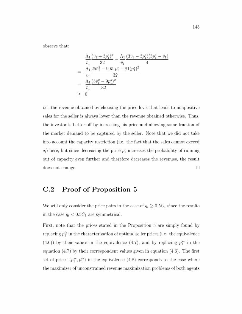
143
observe that:
Λ1
v1
(v1 + 3ps1)2
32− Λ1
v1
(3v1 − 3ps1)(3ps1 − v1)
4
=Λ1
v1
25v21 − 90v1p
s1 + 81(ps1)2
32
=Λ1
v1
(5v21 − 9ps1)2
32
≥ 0
i.e. the revenue obtained by choosing the price level that leads to nonpositive
sales for the seller is always lower than the revenue obtained otherwise. Thus,
the investor is better off by increasing his price and allowing some fraction of
the market demand to be captured by the seller. Note that we did not take
into account the capacity restriction (i.e. the fact that the sales cannot exceed
qi) here; but since decreasing the price pi1 increases the probability of running
out of capacity even further and therefore decreases the revenues, the result
does not change.
C.2 Proof of Proposition 5
We will only consider the price pairs in the case of qi ≥ 0.5C1 since the results
in the case qi < 0.5C1 are symmetrical.
First, note that the prices stated in the Proposition 5 are simply found by
replacing pi∗1 in the characterization of optimal seller prices (i.e. the equivalence
(4.6)) by their values in the equivalence (4.7), and by replacing ps∗1 in the
equation (4.7) by their correspondent values given in equation (4.6). The first
set of prices (ps∗1 , pi∗1 ) in the equivalence (4.8) corresponds to the case where
the maximizer of unconstrained revenue maximization problems of both agents
144
(φ1(.) and φ2(.)) lead to sales figures that are less than the inventories of both
agents. That is, solving pi∗1 =3ps∗1 +v1
8and ps∗1 =
2pi∗1 +v1
6together, we found
that pi∗1 = 9v1
42and ps∗1 = 10v1
42; and the unconstrained sales figures acquire the
values 18Λ1
42and 15Λ1
42for the investors and the seller respectively. The price pair
(ps∗1 , pi∗1 ) = (10v1
42, 9v1
42) is therefore optimal for the ranges of Λ1 values such that
qs ≥ 15Λ1
42and qi ≥ 18Λ1
42. The second set of prices corresponds to the case where
the seller runs out of capacity if she sets the unconstrained revenue maximizing
price; so both prices are adjusted accordingly (i.e. at optimum, the seller’s sales
is exactly equivalent to her inventories; and the investors choose their optimal
best response price that maximizes their unconstrained revenue maximization
problem. That is, ps∗1 = 23( v1
2+ pi∗1 −
v1qsΛ1
) and pi∗1 =3ps∗1 +v1
8). The third case
is symmetrical to the second case, except that now the prices are adjusted
in a way that the sales of investors’ is exactly equivalent to their inventory.
Finally, the fourth set of prices are observed when the market size is very large
and both agents run out of capacity under the revenue maximizing prices of
unconstrained case. Therefore, the prices (ps∗1 , pi∗1 ) are found by solving:
Λ1
v1
(v1 − x(ps∗1 , pi∗1 )) = qs
Λ1
v1
(x(ps∗1 , pi∗1 )− pi∗1 ) = qi
simultaneously.
Observe that the inequality pi∗1 ≤ ps∗1 holds in all cases as claimed in Theorem
7. Moreover, x(ps∗1 , pi∗1 ) ≤ v1 as claimed.
So we only need to show that neither of the agents wants to deviate from
his/her equilibrium price. Since ps∗1 is the seller’s best response price to pi∗1
and so is pi∗1 to ps∗1 given ps∗1 ≥ pi∗1 ; we need to check if there exists some other
price ps1 < pi∗1 where the seller is better off than at ps∗1 , or some price pi1 > ps∗1
145
where the investors have higher revenue than that at pi∗1 . We will analyze all
cases in detail:
• 15Λ1
42≤ qs and 18Λ1
42≤ qi:
Recall that in this case, ps∗1 = 10v1
42, pi∗1 = 9v1
42and x(ps∗1 , p
i∗1 ) = 27v1
42. Thus,
the seller revenue is Πs1(ps∗1 = 10v1
42) = 10v1
4215Λ1
42and the investor revenue
Πi1(pi∗1 = 9v1
42) = 9v1
4218Λ1
42.
First, consider the seller: The revenue maximization problem to find the
revenue maximizing price ps1 < pi∗1 is given by:
maxps1<
9v142
ps1 min{qs,Λ1[
(v1+3
9v142
2− ps1)− ps1v1
]}
which is maximized at ps1 = 23v1
112(provided qs >
69Λ1
168) and the maximum
revenue obtained by setting ps1 ≤ pi∗1 therefore is 23v1
11269Λ1
168. But clearly
23v1
11269Λ1
168< 10v1
4215Λ1
42. Hence, the seller is better off by setting the price
ps∗1 .
Similarly, the revenue maximization problem the investors need to solve
to find the revenue maximizer price pi1 > ps∗1 is given by:
maxpi1>
10v142
pi1 min{qi,Λ1[
v1 − v1+3pi12
+ 10v1
42
v1
]}
which is maximized at pi1 = 31v1
126and the revenue obtained at this price
level is 31v1
12631Λ1
84. But clearly 31v1
12631Λ1
84< 9v1
4218Λ1
42. Hence, the investors are
also better off by setting the price pi∗1 .
• 15Λ1
42> qs and 2
3Λ1 − 2qs
3≤ qi:
Recall that in this case, ps∗1 = 5v1
9− 8qsv1
9Λ1, pi∗1 = v1
3− qsv1
3Λ1and x(ps∗1 , p
i∗1 ) =
v1− qsv1
Λ1. Thus, the seller revenue is Πs
1(ps∗1 = 5v1
9− 8qsv1
9Λ1) = (5v1
9− 8qsv1
9Λ1)qs
146
and the investor revenue assumes the value Πi1(pi∗1 = v1
3− qsv1
3Λ1) = (2Λ1
3−
2qs3
)( v1
3− qsv1
3Λ1).
First, consider the seller: She is already selling all her inventory at the
price ps∗1 > pi∗1 , so decreasing her price below pi∗1 could only lower her
revenues. Thus, given that ps∗1 is her best response price to pi∗1 among
all prices that exceed pi∗1 , she does not deviate.
Next, the revenue maximization problem of the investors to find the
revenue maximizer price pi1 > ps∗1 is given by:
maxpi1>
5v19− 8qsv1
9Λ1
pi1 min{qi,Λ1[
v1 − v1+3pi12
+ 5v1
9− 8qsv1
9Λ1
v1
]}
which is maximized at pi1 = 13(19v1
18− 8qsv1
9Λ1) and the revenue obtained at
this price level is Λ1(1954− 8qs
27Λ1)(19v1
36− 8qsv1
18Λ1). But note that:
(v1
3− qsv1
3Λ1
)(2Λ1
3− 2qs
3)− (
19v1
54− 8qsv1
27Λ1
)(19Λ1
36− 8qs
18)
=Λ1
v1
[2(v1
3− qsv1
3Λ1
)2 − 1
6(19v1
18− 8qsv1
9Λ1
)2]
≥ 0
since:
[2√
3(v1
3− qsv1
3Λ1
)− (19v1
18− 8qsv1
9Λ1
)]
= 0.099v1 − 0.266qsv1
Λ1
≥ 0
which follows from 15Λ1
42> qs. Hence, the investors are also better off by
staying below the price of the seller.
• (Λ1
2− qi
3) ≤ qs and 18Λ1
42> qi:
First, observe that this case is only possible when qi > qs ≥ 5qi6
; i.e.
12C1 ≤ qi ≤ 6
11C1.
147
Recall that in this case, ps∗1 = v1
3− 2qiv1
9Λ1, pi∗1 = v1
2− 2qiv1
3Λ1and x(ps∗1 , p
i∗1 ) =
v1
2+ qiv1
3Λ1. Thus, the seller revenue is Πs
1(ps∗1 = v1
3− 2qiv1
9Λ1) = Λ1
v1
32( v1
3− 2qiv1
9Λ1)2
and the investor revenue Πi1(pi∗1 = v1
2− 2qiv1
3Λ1) = ( v1
2− 2qiv1
3Λ1)qi.
First, consider the seller: The revenue maximization problem she needs
to solve to find the revenue maximizing price ps1 < pi∗1 is given by:
maxps1≤
v12− 2qiv1
3Λ1
ps1 min{qs,Λ1[
(v1+3(
v12− 2qiv1
3Λ1)
2− ps1)− ps1
v1
]}
which is maximized at ps1 = 5v1
16− qiv1
4Λ1provided qs > Λ1(5
8− qi
2Λ1) and at
min{pi∗1 , 5v1
8− v1(qi+qs)
2Λ1} otherwise. There are a few cases to consider:
(i) First, suppose qs >5Λ1
8− qi
2holds. Then, the revenue obtained at
the price ps1 = 5v1
16− qiv1
4Λ1is given by Λ1
v12(5v1
16− qiv1
4Λ1)2. Thus, the seller is
better off by setting the lower price if:
Λ1
v1
2(5v1
16− qiv1
4Λ1
)2 − Λ1
v1
3
2(v1
3− 2qiv1
9Λ1
)2 ≥ 0
⇐⇒ qi ≤ 0.414Λ1
But note that qs < qi and qs >5Λ1
8− qi
2together lead to qi > 0.416Λ1,
which then leads to a contradiction along with the inequality qi ≤
0.414Λ1. Hence, this case cannot hold.
(ii) Next, consider the case where qs <5Λ1
8− qi
2and the revenue maxi-
mizing price is 5v1
8− v1(qi+qs)
2Λ1. Then, 5v1
8− r(qi+qs)
2Λ1≤ pi∗1 = v1
2− 2qir
3Λ1. Along
with the definition of the case range (i.e. Λ1
2− qi
3≤ qs and 18Λ1
42> qi),
and the assumption that qs < qi, it is possible to show that qs ∈
[0.375Λ1, 0.416Λ1]. Then, the difference in revenue figures by setting
the price 5v1
8− v1(qi+qs)
2Λ1and the price ps∗1 is given by:
∆(5v1
8− v1(qi + qs)
2Λ1
,v1
3−2qiv1
9Λ1
) = qs(5v1
8− v1(qi + qs)
2Λ1
)−Λ1
v1
3
2(v1
3−2qiv1
9Λ1
)2
148
It could be shown that the revenue difference ∆(5v1
8− v1(qi+qs)
2Λ1, v1
3− 2qiv1
9Λ1)
is nonpositive for all qs values in the range qs ∈ [0.375Λ1, 0.416Λ1].
(To check this claim, note that ∆ has partial derivative ∂∆∂qs
= 5v1
8−
v1(qi+qs)2Λ1
− 3Λ1
2v12( v1
3− 2(C1−qs)v1
9Λ1) 2v1
9Λ1= 0.403v1− v1
Λ1(0.351(qi+qs)+0.222qs)
(which follows by noting that qi + qs = C1, a fixed value). Moreover,
∂∆∂qs
> 0 for all qs ∈ [0.375Λ1, 0.416Λ1]. Thus, checking the revenue
difference at the maximum value qs could attain, i.e. qs = 0.416Λ1 and
all associated qi ≥ qs values that satisfy the initial assumptions, it could
be verified that the revenue difference ∆(5v1
8− v1(qi+qs)
2Λ1, v1
3− 2qiv1
9Λ1) is
nonpositive.)
Thus, the seller cannot do better by decreasing her price below pi∗1 .
Next, consider the investors: The revenue maximization problem of the
investors to find the revenue maximizer price pi1 > ps∗1 is given by:
maxpi1>
v13− 2qiv1
9Λ1
pi1 min{qi,Λ1[
v1 − v1+3pi12
+ v1
3− 2qiv1
9Λ1
v1
]}
which is maximized at pi1 = 5v1
18− 2qiv1
27Λ1provided that qi ≥ 0.375Λ1. But
note that, the revenue difference:
∆(5v1
18− 2qiv1
27Λ1
,v1
2− 2qiv1
3Λ1
) =1.5Λ1
v1
(5v1
18− 2qiv1
27Λ1
)2 − (v1
2− 2qiv1
3Λ1
)qi
is nonpositive for qi ∈ [0.375Λ1, 0.428Λ1]. If, on the other hand, qi <
0.375Λ1, then the investor revenues are maximized at the price where
investor sales is exactly equivalent to the inventory. But this is already
the case at pi∗1 . Hence, the investors are also better off by staying at the
price level pi∗1 .
• Λ11542> qs and Λ1
1842> qi:
149
Recall that in this case, ps∗1 = v1 − 2(2qs+qi)v1
3Λ1, pi∗1 = v1 − (qi+qs)v1
Λ1and
x(ps∗1 , pi∗1 ) = v1 − qsv1
Λ1. Thus, the seller revenue is Πs
1(ps∗1 ) = qs(v1 −2(2qs+qi)v1
3Λ1) and the investor revenue Πi
1(pi∗1 ) = (v1 − (qi+qs)v1
Λ1)qi.
First, consider the seller: She is already selling all her inventory at the
price ps∗1 > pi∗1 , so decreasing her price below pi∗1 could only lower her
revenues. Thus, given that ps∗1 is her best response price to pi∗1 among
all prices that exceed pi∗1 , she does not deviate.
Next, the revenue maximization problem of the investors to find the
revenue maximizer price pi1 > ps∗1 is given by:
maxpi1>v1−
2(2qs+qi)v13Λ1
pi1 min{qi,Λ1[
v1 − v1+3pi12
+ v1 − 2(2qs+qi)v1
3Λ1
v1
]}
which is maximized at pi1 = v1
2− 2(2qs+qi)v1
9Λ1, provided v1
2− 2(2qs+qi)v1
9Λ1≥
ps∗1 . Otherwise, by concavity of the revenue function, the investors’ best
response price in the range pi1 ≥ ps∗1 is ps∗1 itself, which proves that pi∗1 is
indeed the optimal price to start with. Thus, assume v1
2− 2(2qs+qi)v1
9Λ1≥ ps∗1 ,
i.e. 2qs + qi >98Λ1, which (combined with the fact that qs <
1542
Λ1)
leads to qi ≥ 2356
Λ1. The investor revenues at the price v1
2− 2(2qs+qi)v1
9Λ1is
3Λ1
2v1( v1
2− 2(2qs+qi)v1
9Λ1)2. But note that, the revenue difference:
∆(v1
2− 2(2qs + qi)v1
9Λ1
, v1 −(qi + qs)v1
Λ1
)
=3Λ1
2v1
(v1
2− 2(2qs + qi)v1
9Λ1
)2 − (v1 −(qi + qs)v1
Λ1
)qi
is nonpositive for qi ∈ [2356
Λ1,1842
Λ1], qs < qi and 2qs + qi >98Λ1. Hence,
the investors are again better off by staying below the price of the seller.
A similar result could be established in the cases where Λ11542> qs and Λ1(2
3−
2qs3Λ1
) > qi; and Λ1(12− qi
3Λ1) > qs and Λ1(18
42) > qi along the same lines as
in this case, and we omit the details.
150
�
C.3 Proof of Proposition 7
Consider the centralized pricing problem:
Π1(γ,Λ1, qs, qi) = maxpi1,p
s1
[ps1 min
{qs,Λ1[
v1 − x(ps1, pi1)
v1
]}
+pi1 min{qi,Λ1[
x(ps1, pi1)− pi1v1
]}]
1{ps1≥pi1}
+[ps1 min
{qs,Λ1[
x(pi1, ps1)− ps1v1
]}
+pi1 min{qi,Λ1[
v1 − x(pi1, ps1)
v1
]}]
1{ps1<pi1}
Assume qi > qs. Suppose that the claim of the Proposition 7 holds. Then, the
solution of the above problem is equivalent to the solution of the “Problem 1”
defined as:
Π11(γ,Λ1, qs, qi) = max
pi1,ps1
ps1 min{qs,Λ1[
v1 − x(ps1, pi1)
v1
]}
+pi1 min{qi,Λ1[
x(ps1, pi1)− pi1v1
]}
which can be reformulated as:
Π11(γ,Λ1, qs, qi) = max
ps1≥pi1ps1Λ1[
v1 − x(ps1, pi1)
v1
] + pi1Λ1[x(ps1, p
i1)− pi1v1
]
subject to
Λ1[v1 − x(ps1, p
i1)
v1
] ≤ qs
Λ1[x(ps1, p
i1)− pi1v1
] ≤ qi
Observe that the above formulation is concave in both ps1 and pi1; and its
solution is as follows:
151
• If qs ≥ Λ1323
and qi ≥ Λ1923
, the optimal prices are (ps∗1 , pi∗1 ) = (13
23v1,
1123v1)
and the total system revenue is Π11 = Λ1
623v1.
• If qs < Λ1323
and qi ≥ Λ1
2− 5
6qs, the optimal prices are (ps∗1 , p
i∗1 ) =
(23v1 − 7qsv1
9Λ1, v1
2− qsv1
6Λ1) and the total system revenue is Π1
1 = 16v1qs −
2336
(qs)2v1
Λ1+ Λ1
14v1.
• If qs ≥ Λ138− 5
8qi and qi < Λ1
923
, the optimal prices are (ps∗1 , pi∗1 ) =
( v1
2+ qiv1
6Λ1, 5
8v1 − 3qiv1
8Λ1) and the total system revenue is Π1
1 = 38v1qi −
2348v1(qi)
2
Λ1+ Λ1
316v1.
• If qs < Λ1323
and qi <Λ1
2− 5
6qs; or if qs < Λ1
38− 5
8qi and qi < Λ1
923
; then
the optimal prices are (ps∗1 , pi∗1 ) = (v1 − 2(2qs+qi)v1
3Λ1, v1 − (qi+qs)v1
Λ1) and the
total system revenue is Π11 = qs(v1 − 2(2qs+qi)v1
3Λ1) + qi(v1 − (qi+qs)v1
Λ1).
Next, assume that the claim of the Proposition does not hold; i.e. ps∗1 < pi∗1 .
Then, the solution of the original problem is equivalent to the solution of the
“Problem 2” below:
Π21(γ,Λ1, qs, qi) = max
pi1,ps1
ps1 min{qs,Λ1[
x(pi1, ps1)− ps1v1
]}
+pi1 min{qi,Λ1[
v1 − x(pi1, ps1)
v1
]}
which is equivalent to:
Π21(γ,Λ1, qs, qi) = max
ps1≥pi1ps1Λ1[
x(pi1, ps1)− ps1v1
] + pi1Λ1[v1 − x(pi1, p
s1)
v1
]
subject to
Λ1[v1 − x(pi1, p
s1)
v1
] ≤ qi
Λ1[x(pi1, p
s1)− ps1v1
] ≤ qs
There are again a few cases to consider:
152
• If qi ≥ Λ1323
and qs ≥ Λ1923
, the optimal prices are (ps∗1 , pi∗1 ) = (11
23v1,
1323v1)
and the total system revenue is Π21 = Λ1
623v1.
• If qi < Λ1323
and qs ≥ Λ1
2− 5
6qi, the optimal prices are (ps∗1 , p
i∗1 ) =
( v1
2− qiv1
6Λ1, 2
3v1 − 7qsv1
9Λ1) and the total system revenue is Π2
1 = 16v1qi −
2336
(qi)2v1
Λ1+ Λ1
14v1. (However, this case is never attained for qi > qs.)
• If qi ≥ Λ138− 5
8qs and qs < Λ1
923
, the optimal prices are (ps∗1 , pi∗1 ) =
(58v1 − 3qsv1
8Λ1, v1
2+ qsv1
6Λ1) and the total system revenue is Π2
1 = 38v1qs −
2348v1(qs)2
Λ1+ Λ1
316v1.
• If qi < Λ1323v1 and qs <
Λ1
2− 5
6qi; or if qi < Λ1
38− 5
8qs and qs < Λ1
923
;
then the optimal prices are (ps∗1 , pi∗1 ) = (v1− (qi+qs)v1
Λ1, v1− 2(2qi+qs)v1
3Λ1) and
the total system revenue is Π21 = qi(v1 − 2(2qi+qs)v1
3Λ1) + qs(v1 − (qi+qs)v1
Λ1).
Observe that some of the cases in the characterization of Π21 can never be
attained for qi > qs. Combining the two analyses, the comparison of optimal
values of Problem 1 and Problem 2 are as following:
• If both qi > Λ1923
and qs > Λ1923
, the optimal solutions of the two
problems are equivalent; i.e. Π11 = Π2
1 = Λ1623v1.
• If qi > Λ1923
but Λ1323< qs < Λ1
923
, then Π11 = Λ1
623v1 but Π2
1 = 38v1qs −
2348v1(qs)2
Λ1+Λ1
316v1. It could be shown that Π1
1 ≥ Π21 for this range of (qi, qs)
values by noting that the function Π21 increases in qs for qs ∈ (Λ1
323,Λ1
923
)
and attains it maximum value which is equivalent to Π11 at qs = Λ1
923
.
• If Λ1323< qs < qi < Λ1
923
, then Π11 = 3
8v1qi− 23
48v1(qi)
2
Λ1+Λ1
316v1. There are
two cases for the second problem: If qi ≥ Λ138− 5
8qs, then Π2
1 = 38v1qs −
2348v1(qs)2
Λ1+ Λ1
316v1. Otherwise, Π2
1 = qi(v1− 2(2qi+qs)v1
3Λ1) + qs(v1− (qi+qs)v1
Λ1).
153
By noting that qi(v1− 2(2qi+qs)v1
3Λ1) + qs(v1− (qi+qs)v1
Λ1) ≤ 3
8v1qs− 23
48v1(qs)2
Λ1+
Λ1316v1 for qi < Λ1
38− 5
8qs and that the function ζ(x) = 3
8v1x− 23
48v1x2
Λ1+
Λ1316v1 is increasing in the range x ∈ (Λ1
323,Λ1
923
), it could be shown
that Π11 ≥ Π2
1 in both cases.
• If qs < Λ1323< qi < Λ1
923
, there are three cases:
– If qi < Λ138− 5
8qs, then Π1
1 = qs(v1− 2(2qs+qi)v1
3Λ1)+qi(v1− (qi+qs)v1
Λ1) and
Π21 = qi(v1 − 2(2qi+qs)v1
3Λ1) + qs(v1 − (qi+qs)v1
Λ1). It could be shown that
Π11 ≥ Π2
1 for this range of (qi, qs) values, since (v1 − 2(2qi+qs)v1
3Λ1) <
(v1 − (qi+qs)v1
Λ1) < (v1 − 2(2qs+qi)v1
3Λ1) and qs < qi.
– If Λ138− 5
8qs ≤ qi < Λ1
12− 5
8qs, then Π1
1 = qs(v1− 2(2qs+qi)v1
3Λ1)+qi(v1−
(qi+qs)v1
Λ1) and Π2
1 = 38v1qs − 23
48v1(qs)2
Λ1+ Λ1
316v1. It could be shown
that Π11 ≥ Π2
1 for this range of (qi, qs) values.
– If qi ≥ Λ112− 5
8qs, then Π1
1 = 16v1qs − 23
36v1(qs)2
Λ1+ Λ1
14v1 and Π2
1 =
38v1qs − 23
48v1(qs)2
Λ1+ Λ1
316v1. It could be shown that Π1
1 ≥ Π21 for
qs < Λ1323
.
• If qs < Λ1323< Λ1
923< qi, there are two cases:
– If Λ138− 5
8qs ≤ qi < Λ1
12− 5
8qs, then Π1
1 = qs(v1− 2(2qs+qi)v1
3Λ1)+qi(v1−
(qi+qs)v1
Λ1) and Π2
1 = 38v1qs − 23
48v1(qs)2
Λ1+ Λ1
316v1. It could be shown
that Π11 ≥ Π2
1 for this range of (qi, qs) values.
– If qi ≥ Λ112− 5
8qs, then Π1
1 = 16v1qs − 23
36v1(qs)2
Λ1+ Λ1
14v1 and Π2
1 =
38v1qs − 23
48v1(qs)2
Λ1+ Λ1
316v1. It could be shown that Π1
1 ≥ Π21 for
qs < Λ1323
.
• If qs < qi < Λ1323
, then then Π11 = qs(v1− 2(2qs+qi)v1
3Λ1)+qi(v1− (qi+qs)v1
Λ1) and
Π21 = qi(v1− 2(2qi+qs)v1
3Λ1) + qs(v1− (qi+qs)v1
Λ1). It is easy to see that Π1
1 ≥ Π21
154
for this range of (qi, qs) values since (v1 − 2(2qi+qs)v1
3Λ1) < (v1 − (qi+qs)v1
Λ1) <
(v1 − 2(2qs+qi)v1
3Λ1).
Hence, in all cases the optimal value attained in the first problem is greater
than or equal to the optimal value of the second problem. Therefore, the
formulation (4.14) could be reduced to the problem defined as Problem 1;
which proves the claim of the Proposition.
�


