

. . . . . .
.
.
. ..
.
.
Information Theory: Principles and Applications
Tiago T. V. Vinhoza
April 9, 2010
Tiago T. V. Vinhoza () Information Theory - MAP-Tele April 9, 2010 1 / 42
. . . . . .
.. .1 AEP and Source Coding
.. .2 Markov Sources and Entropy Rate
.. .3 Other Source CodesShannon-Fano-Elias codesArithmetic CodesLempel-Ziv Codes
.. .4 Channel CodingTypes of ChannelChannel Capacity
Tiago T. V. Vinhoza () Information Theory - MAP-Tele April 9, 2010 2 / 42
. . . . . .
AEP and Source Coding
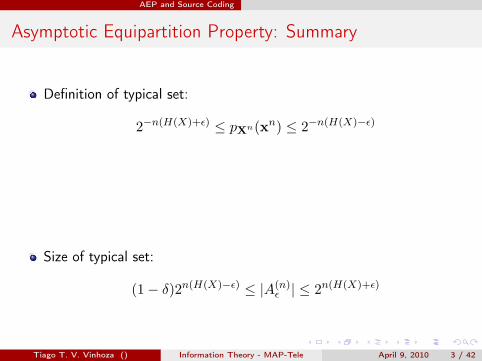
Asymptotic Equipartition Property: Summary
Definition of typical set:
2−n(H(X)+ϵ) ≤ pXn(xn) ≤ 2−n(H(X)−ϵ)
Size of typical set:
(1 − δ)2n(H(X)−ϵ) ≤ |A(n)ϵ | ≤ 2n(H(X)+ϵ)
Tiago T. V. Vinhoza () Information Theory - MAP-Tele April 9, 2010 3 / 42

. . . . . .
AEP and Source Coding
Source coding in the light of the AEP
A source coder operating on strings of n source symbols need onlyprovide a codeword for each string xn in the typical set A
(n)ϵ .
If a sequence xn occurs that is not the typical set A(n)ϵ , then a source
coding failure is declared.The probability of failure can be made arbitrarily small by choosing an large enough.
Since |A(n)ϵ | ≤ 2n(H(X)+ϵ), the number of source codewords that need
to be provided is fewer than 2n(H(X)+ϵ).So, fixed length codewords of length ⌈n(H(X) + ϵ)⌉ is enough.
L ≤ H(X) + ϵ + 1/n
Tiago T. V. Vinhoza () Information Theory - MAP-Tele April 9, 2010 4 / 42

. . . . . .
AEP and Source Coding
Source coding theorem
For any discrete memoryless source with entropy H(X), any ϵ > 0,any δ > 0, and any sufficiently large n, there is a fixed-to-fixed-lengthsource code with P (failure) ≤ δ that maps blocks of n source symbolsinto fixed-length codewords of length L ≤ H(X) + ϵ + 1/n bps.Compare this result with log M for fixed-length source codes withoutfailures.
Tiago T. V. Vinhoza () Information Theory - MAP-Tele April 9, 2010 5 / 42

. . . . . .
AEP and Source Coding
Source coding theorem: converse
Let Xn be a string of n discrete random variables Xi, i = 1, . . . , neach with entropy H(X). For any ν > 0, let Xn be encoded intofixed-length codewords of length ⌊n(H(X) − ν)⌋ bits. For any δ > 0and for all sufficiently large n,
P (failure) > 1 − δ − 2−νn/2
Going from a fixed-length code with codeword lengths slightly largerthan the entropy to a fixed-length code with codeword lengths slightlysmaller than the entropy makes the probability of failure jump fromalmost 0 to almost 1.
Tiago T. V. Vinhoza () Information Theory - MAP-Tele April 9, 2010 6 / 42

. . . . . .
Markov Sources and Entropy Rate
Sources with dependent symbols
AEP established that nH(X) bits is enough, on average, to describe nindependent and identically distributed random variables.What happens when the variables are dependent?What if the sequence of random variables form a stationary stochasticprocess?
Tiago T. V. Vinhoza () Information Theory - MAP-Tele April 9, 2010 7 / 42

. . . . . .
Markov Sources and Entropy Rate
Stochastic Processes
A stochastic process is an indexed sequence of random variables.Characterized by the joint probability distributionpX1,...,Xn(x1, . . . , xn). where (x1, . . . , xn) ∈ X n
Tiago T. V. Vinhoza () Information Theory - MAP-Tele April 9, 2010 8 / 42

. . . . . .
Markov Sources and Entropy Rate
Stochastic Processes
Stationarity: Joint probability distribution does not change withtime-shifts.
pX1+d,...,Xn+d(x1, . . . , xn) = pX1,...,Xn(x1, . . . , xn)
for every shift d and for all where x1, . . . , xn ∈ X
Tiago T. V. Vinhoza () Information Theory - MAP-Tele April 9, 2010 9 / 42

. . . . . .
Markov Sources and Entropy Rate
Markov Process or Markov Chain
Each random variable depends on the one preceding it and isconditionally independent of all other preceding random variables.
P (Xn+1 = xn+1|Xn = xn, . . . X1 = x1) = P (Xn+1 = xn+1|Xn = xn)
for all where x1, . . . , xn+1 ∈ XJoint probability distribution
pX1,...,Xn(x1, . . . , xn) = pX1(x1)pX2|X1=x1(x2)pX3|X2=x2
(x3) . . . pXn|Xn−1=xn−1(xn)
Tiago T. V. Vinhoza () Information Theory - MAP-Tele April 9, 2010 10 / 42

. . . . . .
Markov Sources and Entropy Rate
Markov Process or Markov Chain
A Markov chain is irreducible if it is possible to go from any state toany other state in a finite number of stepsA Markov chain is time invariant if the conditional probability does notdepend on the time index n.
P (Xn+1 = a|Xn = b) = P (X2 = a|X1 = b)
for all a, b ∈ X .Xn is the state of the Markov chain in time n.
Tiago T. V. Vinhoza () Information Theory - MAP-Tele April 9, 2010 11 / 42

. . . . . .
Markov Sources and Entropy Rate
Markov Process or Markov Chain
A time invariant Markov chain is characterized by its initial state and aprobability transition matrix P, whose element (i, j) is given by
P (Xn+1 = j|Xn = i)
Stationary distributions
Tiago T. V. Vinhoza () Information Theory - MAP-Tele April 9, 2010 12 / 42

. . . . . .
Markov Sources and Entropy Rate
Entropy Rate
Given a sequence of random variables X1, X2, . . . , Xn.How does the entropy of the sequence grows with n?The entropy rate is defined as this rate of growth.
H(X ) = limn→∞
1n
H(X1, X2, . . . , Xn)
when the limit exists.
Tiago T. V. Vinhoza () Information Theory - MAP-Tele April 9, 2010 13 / 42
. . . . . .
Markov Sources and Entropy Rate
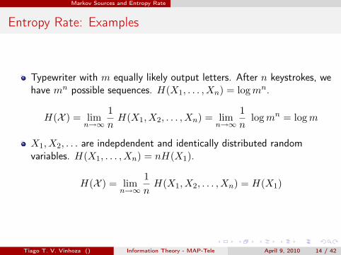
Entropy Rate: Examples
Typewriter with m equally likely output letters. After n keystrokes, wehave mn possible sequences. H(X1, . . . , Xn) = log mn.
H(X ) = limn→∞
1n
H(X1, X2, . . . , Xn) = limn→∞
1n
log mn = log m
X1, X2, . . . are indepdendent and identically distributed randomvariables. H(X1, . . . , Xn) = nH(X1).
H(X ) = limn→∞
1n
H(X1, X2, . . . , Xn) = H(X1)
Tiago T. V. Vinhoza () Information Theory - MAP-Tele April 9, 2010 14 / 42

. . . . . .
Markov Sources and Entropy Rate
Entropy Rate
Other definition of entropy rate:
H ′(X ) = limn→∞
H(Xn|Xn−1, . . . , X1)
when the limit exists.For stationary stochastic processes H(X ) = H ′(X )For a stationary Markov chain H(X ) = H(X2|X1).
Tiago T. V. Vinhoza () Information Theory - MAP-Tele April 9, 2010 15 / 42

. . . . . .
Markov Sources and Entropy Rate
Why entropy rate is important?
There is a version of the AEP for stationary ergodic sources.
− 1n
pXn(xn) → H(X )
Like the AEP presented last class: 2nH(X ) typical sequences withprobability 2−nH(X )
We can represent typical sequences of length n using nH(X ) bits.
Tiago T. V. Vinhoza () Information Theory - MAP-Tele April 9, 2010 16 / 42

. . . . . .
Other Source Codes
Other Source Codes
Shannon-Fano-Elias codes.Arithmetic codes.Lempel-Ziv codes.
Tiago T. V. Vinhoza () Information Theory - MAP-Tele April 9, 2010 17 / 42

. . . . . .
Other Source Codes Shannon-Fano-Elias codes
Shannon-Fano-Elias Codes
Simple encoding procedure based on the cumulative distributionfunction (CDF) to allot codewords.
FX(x) =∑a≤x
pX(a)
Modified CDF
FX(x) =∑a<x
pX(a) +12; P (X = x)
FX(x) is known, x is known.
Tiago T. V. Vinhoza () Information Theory - MAP-Tele April 9, 2010 18 / 42

. . . . . .
Other Source Codes Shannon-Fano-Elias codes
Shannon-Fano-Elias Codes
From last class: We know that l(xi) = − log pX(xi) gives good codes.Use binary expansion of FX(x) as code for x. Rounding needed. Wewill round to ∼ − log pX(xi).Use base 2 fractions.
z ∈ [0, 1) → z =∞∑i=1
zi2−i
Taking the first k bits ⌊z⌋k = z1z2 . . . zk, zi ∈ {0, 1}.Example: 2/3 = 0.10101010 . . . = 0.10 → ⌊2/3⌋5 = 10101
Tiago T. V. Vinhoza () Information Theory - MAP-Tele April 9, 2010 19 / 42

. . . . . .
Other Source Codes Shannon-Fano-Elias codes
Shannon-Fano-Elias Codes
Coding procedure
l(xi) =⌈log
1pX(xi)
⌉+ 1
C(xi) = ⌊FX(xi)⌋l(xi)
Tiago T. V. Vinhoza () Information Theory - MAP-Tele April 9, 2010 20 / 42

. . . . . .
Other Source Codes Shannon-Fano-Elias codes
Shannon-Fano-Elias Codes
Example:pX(xi) l(xi) FX(xi) C(xi)
x1 1/3 3 1/6 001x2 1/6 4 5/12 0110x3 1/6 4 7/12 1001x4 1/3 3 5/6 110
Tiago T. V. Vinhoza () Information Theory - MAP-Tele April 9, 2010 21 / 42

. . . . . .
Other Source Codes Shannon-Fano-Elias codes
Dyadic Intervals
A binary string can represent a subinterval of [0, 1)From the usual binary representation of a number
z1z2 . . . zn ∈ {0, 1}m → z =m∑
i=1
zi2m−i ∈ {0, 1, . . . , 2m − 1}.
We get
z1z2 . . . zn →[
z
2m,z + 12m
)Example: 110 → [3/4, 7/8).Codewords of Shannon-Fano-Elias code are disjoint intervals.
Tiago T. V. Vinhoza () Information Theory - MAP-Tele April 9, 2010 22 / 42

. . . . . .
Other Source Codes Arithmetic Codes
Arithmetic Codes
Arithmetic Codes: invented by Elias, by Rissanen and by Pasco, andmade practical by Witten et al in 1987.More practical than Huffman coding for large number of sourcesymbols.Why? Huffman need to generate and store all codewords.Arithmetic Code generate codeword without needing to compute allthe others.Protected by several US patents: not widely used.Original bzip used an arithmetic coder, its replacement bzip2employed a Huffman coder.Based on Shannon-Fano-Elias code.
Tiago T. V. Vinhoza () Information Theory - MAP-Tele April 9, 2010 23 / 42

. . . . . .
Other Source Codes Arithmetic Codes
Arithmetic Codes
Example: Discrete memoryless source X ∈ {1, 2, 3, 4}p1 = 0.25, p2 = 0.5, p3 = 0.2 and p4 = 0.05.We want the binary codeword for 2313.
Tiago T. V. Vinhoza () Information Theory - MAP-Tele April 9, 2010 24 / 42

. . . . . .
Other Source Codes Lempel-Ziv Codes
Lempel-Ziv Codes
Do not require knowledge of the source statistics. They adapt so thatthe average codeword length L per source-symbol is minimized insome sense.Such algorithms are called universal.Widely used in practice.
Tiago T. V. Vinhoza () Information Theory - MAP-Tele April 9, 2010 25 / 42

. . . . . .
Other Source Codes Lempel-Ziv Codes
Lempel-Ziv Codes: Algorithms
LZ77: string-matching on a sliding window.Most popular LZ77 based compression method is called DEFLATE; itcombines LZ77 with Huffman coding.LZ78: adaptive dictionary.UNIX compress is based on LZ78.A lot of variants: LZW, LZWA.
Tiago T. V. Vinhoza () Information Theory - MAP-Tele April 9, 2010 26 / 42
. . . . . .
Other Source Codes Lempel-Ziv Codes
Lempel-Ziv Codes: LZ78 Example
String: 1011010100010
Encoded String: 100011101100001000010
Tiago T. V. Vinhoza () Information Theory - MAP-Tele April 9, 2010 27 / 42

. . . . . .
Other Source Codes Lempel-Ziv Codes
Lempel-Ziv Codes: LZ78 Example
String: 1011010100010Encoded String: 100011101100001000010
Tiago T. V. Vinhoza () Information Theory - MAP-Tele April 9, 2010 27 / 42

. . . . . .
Channel Coding Types of Channel
Communications Channel
Channel: source of randomness (interference, fading, noise, etc.).Random nature of the channel is described by a probabilitydistribution over the output of the channel.That distribution will often be dependent on the input chosen to betransmitted.Discrete case: Both input and output symbols belong to a finitealphabet.
Tiago T. V. Vinhoza () Information Theory - MAP-Tele April 9, 2010 28 / 42

. . . . . .
Channel Coding Types of Channel
Discrete Channel
If we apply a sequence x1, x2, . . . , xn from an alphabet X at the inputof a channel, then at the output we will receive a sequencey1, y2, . . . , yn belonging to an alphabet Y.Usually the probability distribution over the outputs depend on theinput and on the state of the channel.Some channels have memory. For example, the output symbol yn
might be dependent on previous inputs or outputs.Causal behavior: In general y1, y2, . . . , yn do not need to considerinputs beyiond x1, y2, . . . , xn.
Tiago T. V. Vinhoza () Information Theory - MAP-Tele April 9, 2010 29 / 42

. . . . . .
Channel Coding Types of Channel
Discrete Channel
Given an input alphabet X , an output alphabet Y and a set of statesS, a discrete channel is defined as a system of conditional probabilitydistributions
P (y1, y2, . . . , yn|x1, x2, . . . , xn; s)
where x1, x2, . . . , xn ∈ X , y1, y2, . . . , yn ∈ Y and s ∈ S.P (y1, y2, . . . , yn|x1, x2, . . . , xn; s) can be interpreted as the probabilitythat the sequence y1, y2, . . . , yn will appear at the output of thechannel if the sequence x1, x2, . . . , xn is applied at the input and theinitial state of the channel is s.Initial state here is defined as the state before applying x1 at the input.
Tiago T. V. Vinhoza () Information Theory - MAP-Tele April 9, 2010 30 / 42

. . . . . .
Channel Coding Types of Channel
Discrete Memoryless Channel
A discrete channel is memoryless ifP (y1, y2, . . . , yn|x1, x2, . . . , xn; s) does not depend on s so it can bewritten as P (y1, y2, . . . , yn|x1, x2, . . . , xn)P (y1, y2, . . . , yn|x1, x2, . . . , xn) = P (y1|x1) P (y2|x2) . . . P (yn|xn).where x1, x2, . . . , xn ∈ X , y1, y2, . . . , yn ∈ Y and s ∈ S.
Tiago T. V. Vinhoza () Information Theory - MAP-Tele April 9, 2010 31 / 42
. . . . . .
Channel Coding Channel Capacity
Information Processed by a Channel
Let the input uncertainty be H(X), H(Y ) is the output uncertaintyand the conditional uncertainties H(X|Y ) and H(Y |X). We definethe information processed by the channel as
I(X; Y ) = H(X) − H(X|Y ) = H(Y ) − H(Y |X)
The information processed by a channel depends on the inputdistribution pX(x).We may vary the input distribution until the information reaches amaximum; the maximum information is called the channel capacity.
C = maxpX(x)
I(X; Y ).
Tiago T. V. Vinhoza () Information Theory - MAP-Tele April 9, 2010 32 / 42
. . . . . .
Channel Coding Channel Capacity
Channel Capacity
Properties of channel capacityC ≥ 0, since I(X; Y ) ≥ 0.C ≤ log |X |, since C = max I(X; Y ) ≤ maxH(X) = log |X |C ≤ log |Y|, for the same reason.I(X;Y ) is a continuous function on pX(x).I(X;Y ) is a concave function of pX(x).
Global maximum.Convex optimization techniques.Blahut-Arimoto algorithm
Tiago T. V. Vinhoza () Information Theory - MAP-Tele April 9, 2010 33 / 42

. . . . . .
Channel Coding Channel Capacity
Classification of Channels
A channel is lossless if H(X|Y ) = 0 for all input distributions.Input is determined from the output and no transmission errors canoccur.A channel is deterministic if P (Y = yi|X = xj) = 1 or 0 for all i, j.The output is determined by the input, that is, H(Y |X) = 0 for allinput distributions.A channel is noiseless is is lossless and deterministic.A channel is useless (or zero-capacity) if I(X; Y ) = 0 for all inputdistributions. Input X and output Y are independent.
Tiago T. V. Vinhoza () Information Theory - MAP-Tele April 9, 2010 34 / 42

. . . . . .
Channel Coding Channel Capacity
Symmetric Channels
A channel is symmetric if the rows of the channel transition matrix arepermutations of each other, and the column are permutations of eachother
P (Y |X) =[
1/3 1/3 1/6 1/61/6 1/6 1/3 1/3
]
P (Y |X) =
1/2 1/3 1/61/6 1/2 1/31/3 1/6 1/2
The entry at the i-th row and j-th column denotes the conditionalprobability P (Y = yj |X = xi) that yj is received given that xi wassent.
Tiago T. V. Vinhoza () Information Theory - MAP-Tele April 9, 2010 35 / 42

. . . . . .
Channel Coding Channel Capacity
Symmetric Channels
A channel is weakly symmetric if the rows of the channel transitionmatrix are permutations of each other, and the sums of the columnsare equal.
P (Y |X) =[
1/3 1/6 1/21/3 1/2 1/6
]
Tiago T. V. Vinhoza () Information Theory - MAP-Tele April 9, 2010 36 / 42

. . . . . .
Channel Coding Channel Capacity
Binary Symmetric Channels
It is the basic example of a noisy communication systemBinary input and binary output. The output is equal to the input withprobability 1 − p. With probability p a 0 is received as 1, andvice-versa.
P (Y |X) =[
1 − p pp 1 − p
]
Tiago T. V. Vinhoza () Information Theory - MAP-Tele April 9, 2010 37 / 42

. . . . . .
Channel Coding Channel Capacity
Binary Erasure Channel
Bits are lost instead of being flipped.A fraction α of bits is lost and the receiver knows that a bit wassupposed to arrive.Packet communications
P (Y |X) =[
1 − α α 00 α 1 − α
]
Tiago T. V. Vinhoza () Information Theory - MAP-Tele April 9, 2010 38 / 42

. . . . . .
Channel Coding Channel Capacity
Channel Capacity: Toy Examples
Noiseless Binary ChannelOne error-free bit can be transmitted per use of the channel.C = 1 bit, and is achieved with uniform input distribution.
Lossless channelInput can be determined from the output. Every transmitted bit can berecovered without error.For our example, C = 1 bit, and is achieved with uniform inputdistribution.
Noisy TypewriterChannel input is either received unchanged at the output withprobability 1/2 or it is transformed to the next letter with probability1/2. That is, if A is transmitted, we can receive A or B. Each withprobability 1/2.Input has 26 symbols. If we use alternate input symbols (A, C, E), wecan transmit 13 symbols without error.
C = max H(Y ) − H(Y |X) = max H(Y ) − 1 = log 26 − 1 = log 13.
Tiago T. V. Vinhoza () Information Theory - MAP-Tele April 9, 2010 39 / 42

. . . . . .
Channel Coding Channel Capacity
Channel Capacity for BSC
Bounding the mutual information for the BSC:
I(X;Y ) = H(Y ) − H(Y |X)
= H(Y ) −∑x∈X
H(Y |X = x)pX(x)
= H(Y ) −∑x∈X
H(p)pX(x)
= H(Y ) − H(p)≤ 1 − H(p)
Equality is achieved when the input distribution is uniform.
C = 1 − H(p)
Tiago T. V. Vinhoza () Information Theory - MAP-Tele April 9, 2010 40 / 42

. . . . . .
Channel Coding Channel Capacity
Channel Capacity for BEC
C = 1 − α.This result is somewhat intuitive: since a fraction α of the input bits iserased, we can recover (at most) 1 − α of the bits.
Tiago T. V. Vinhoza () Information Theory - MAP-Tele April 9, 2010 41 / 42

. . . . . .
Channel Coding Channel Capacity
Why the channel capacity is important?
Shannon proved that the channel capacity is the maximum number ofbits that can be reliably transmitted over the channel.Reliably = probability of error can be made arbitrarily small.Channel coding theorem.
Tiago T. V. Vinhoza () Information Theory - MAP-Tele April 9, 2010 42 / 42


