

Towards Variability ManagementIn Bidirectional Model Transformation
Xiao HeSchool of Computer and Communication
Engineering, University of Science and
Technology Beijing, Beijing 100083, China
Email: [email protected]
Zhenjiang HuNational Informatics Institute, Tokyo, Japan
Email: [email protected]
Yi LiuNational Computer Network
Emergency Response Technical
Team/Coordination Center of China
Abstract—The bidirectional model transformation (BX) com-prises a forward transformation get and a backward transfor-mation put. Given that get may be an information-loss trans-formation, the behavior of put may be uncertain. An uncertainput produces many valid outputs that fit different applicationscenarios. This paper proposes an approach to variability man-agement in BX to enable put to generate an output model withseveral variation points that can be configured to adapt thisoutput for different uses. Firstly, this paper proposes a variabilitymetamodel and management framework, which are used tocharacterize and configure variation points in a transformationresult model. Secondly, this paper extends a BX language tospecify a BX with variability. Thirdly, this paper presents a BXengine, which can execute a BX with variability and generatea model that contains variation points. Lastly, an evaluation ispresented to show the feasibility and scalability of our approach.
I. INTRODUCTION
In Model-Driven Engineering, there is an increasing need
for model synchronization [1], [2], [3], [4] to support iterative,
collaborative, and/or multi-view development, in which the
models that are created at different development phases, by
different developers and/or from different views of the same
system, must be synchronized.
Bidirectional model transformation (BX) [5], [6], [7], [8]
is a promising solution to model synchronization and has
attracted many attentions from academia [9]. A BX can be
defined either asymmetrically or symmetrically. Without losing
generality, this paper adopts the asymmetric definition [10] that
defines a BX as the following pair of functions:
get : S → Vput : S × V → S
where, the forward transformation (get) produces a view
model from a source model, and the backward transformation
(put) converts the original source model and the updated
view model into an updated source model. With regard to the
symmetric case [6], we can combine two asymmetric BXs to
realize a symmetric BX.
In practice, get can be an information-loss transformation,
and consequently, the behavior of put becomes uncertain. Take
the classic transformation UMLtoRDBMS [11] between UML
Class Diagram and Relational Database Management System
(RDBMS) model as an example. The forward transformation
<<table>> e1’
<<class>><<persistent>>
e1
<<class>><<persistent>>
e1<<table>>
e1’
DEL
variant 1 variant 2
DEL
source view
original
updated
get
put<<class>>
<<non-persistent>>e1
Fig. 1: Example of uncertainty
converts all persistent classes into tables. Nevertheless, as
shown in Fig. 1, the deletion of a table may be propagated back
to the Class Diagram at least in the following two ways: 1)
deleting the class that corresponds to this table, or 2) changing
the corresponding class into a non-persistent class.
These two variants of propagating the deletion of a table, as
in Fig. 1, may be applied in different scenarios. Consider the
following example scenarios: 1) Scenario 1 adopts variant 1
that deletes all the classes whose counterparts are deleted; 2)
Scenario 2 adopts variant 2 that changes all the classes whose
counterparts are deleted into non-persistent classes; And 3)
scenario 3 combines variants 1 and 2 that delete some of the
classes, whose counterparts are deleted, while convert the rest
into non-persistent classes.
Intuitively, we can develop three separate BXs to cover the
above three scenarios. Nevertheless, this solution suffers from
high development costs and poor maintainability.
In conventional software engineering, the concept of vari-ability has been proven in practice an effective technique that
enables an application to be configured for use in different
contexts [12]. This paper attempts to adapt software variability
for (bidirectional) model transformation so that a single BX
can be used in different scenarios.
This paper proposes model transformation variability by
adapting software variability. Transformation variability can
be defined at two different levels, namely, the specification
and the instance levels, as follows:
• The specification-level variability is the ability of a
transformation specification to be configured for use in a
specific context, e.g., [13], [14].
2017 IEEE 41st Annual Computer Software and Applications Conference
0730-3157/17 $31.00 © 2017 IEEE
DOI 10.1109/COMPSAC.2017.252
224
• The instance-level variability is the ability of the trans-
formation output to be configured for use in a specific
context, e.g., [15].
The specification-level variability implies that a transfor-
mation specification contains several variation points. We
can change the behavior of this model transformation via
configuring these variation points.
The instance-level variability means that a model transfor-
mation can produce a model that contains several variation
points We can configure these variation points to adapt the
output model for different uses.
This paper focuses on the instance-level variability within
the context of bidirectional model transformation. Firstly, we
propose a variability metamodel that is adapted from COVA-
MOF [16], a well-established conceptual model of software
variability. Secondly, we extend our BX language and engine
to support instance-level variability. The extended language
and engine can declare and produce instance-level variation
points during backward transformation. We also propose a
variability management framework that is used to configure
instance-level variation points in transformation output model.
There is another concept, called ambiguity that is similar
to but different from variability discussed in this paper. Both
ambiguity and variability originate from the nature of uncer-
tainty. However, variability refers to intentional, useful, and
controlled uncertain features in a BX, but ambiguity represents
unintentional and uncontrolled features.
The rest of this paper is structured as follows: Section
II introduces the basic concepts and presents the motivating
example; Section III presents our approach to transformation
variability management and demonstrates how to integrate the
approach into bidirectional model transformation; Sections IV
and V present our tool support and evaluation of our approach;
Section VI discusses the related research efforts; The last
section concludes the paper and the future work.
II. BACKGROUND AND MOTIVATION
A. Bidirectional Model Transformation
A bidirectional model transformation converts a source
model into a view model, and vice-versa. We can straight-
forwardly realize a BX using two separate unidirectional
transformations. Such realization is difficult to assure the
round-trip properties (discussed in Section III-D) of this BX,
therefore systematical BX approaches that make BX easy and
maintainable have been actively studied within the past decade.
There are three major systematical BX approaches, namely,
the relation-based, get-based and putback-based.
Relation-based approaches (e.g., [3], [5], [7]) specify a BX
as a set of bidirectional consistency relations between the
source and view models. Afterwards, a pair of forward and
backward transformations (get and put), which satisfies round-
trip properties, is automatically derived from these consistency
relations. Get-based approaches (e.g., [4]) specify a BX using
a forward transformation (i.e., get), and then automatically
derives the corresponding put from get. The relation-based and
get-based approaches usually suffer from ambiguity problems
[17], [10] that hinder developers from controlling the behavior
of their BXs.
Putback-based bidirectional programming [10] has been
proposed to tackle ambiguity problems. BiFluX [8], a putback-
based BX language for XML, has been designed based on put-back-based bidirectional programming. The key of a putback-
based bidirectional programing is to describe how to update
source model according to an updated view model. A putback-
based BX is specified in the form of a backward transformation
put. The putback-based BX is free from ambiguity problems
because a unique get can always be derived from a well-
defined put [10]. Putback-based bidirectional programming
offers developers full control over the BX behavior.
We adapted BiFluX for bidirectional model transformation
by combining BiFluX with OCL. Our language, which is the
base of this paper, adopts the core language of BiFluX to
interpret a BX over models, while OCL instead of XPath is
used to specify the patterns and the expressions of models.
Listing 1: Example rule of putback-based BX
rule class2table(source p : Package, view s : Schema) {cn : String;update p:Package{classes=c:Class{name=cn, persistent=true,
abstract=false}}with s:Schema{tables=t:Table{name=cn}} bymatch-> attribute2column(c, t)unmatchs-> delete c
/* ALTERNATIVE:unmatchs-> enforce c:Class{persistent=false}
*/unmatchv-> enforce c:Class{name=cn,persistent=true, abstract=false}
}
Listing 1 shows a putback rule defined in our BX language,
which specifies how to update a class using a table. The rule
means that a persistent class c in the package p must be
updated by a table t in the schema s, where the names of
c and t must be identical. If such table t exists, then go on
updating the attributes of c with the columns of t by calling
the rule attribute2column (i.e., the match clause). If
such table is missing, then delete class c in the result (i.e., the
unmatchs clause). If such class is missing, then create a new
class c (i.e., the unmatchv clause) and go on excuting the
match clause. Assuming that we want to change class c into a
non-persistent class when the corresponding table is missing,
we replace the unmatchs clause with the ALTERNATIVEline of code in Listing 1.
B. Variability Management and COVAMOF
In COVAMOF [16], one of the major concepts is the
variation point. Variation points are places in software artifacts
that identify locations at which variation occurs [18]. Each
variation point is associated with a set of variants. Each variant
represents an alternative structure of the associated variation
point. A variant may require or exclude other variants. Those
types of dependencies among variants restrict variant selection.
The variability of a software artifact can be represented
as a variability model that defines a set of variation points.
Configuring a variability model is to select a variant for each
variation point.
225

<<table>>e3’
<<table>>e2’
l1l2
DEL DEL
VP1 VP2
VP3 VP4V1.1
V1.2
V2.1
V2.2V3.1
V3.2
V4.1
V4.2
delete
keep
delete
keepdelete
keep
delete
keep
put
configuration 1
configuration 2
configuration n
l1
l2
……
……
RDBMS Model (view model)
Class Diagram (intermediate output)
Variability Model
Class Diagram (final output after configuration)
Variation Point
Variant
Dependency (Require)
<<table>>e1’
<<class>>e1
<<class>>e2
<<class>>e3 <<class>>
e1<<class>>
e2
<<class>>e1
<<class>>e2
<<class>>e3
Fig. 2: Running example
C. Running Example
This paper uses the transformation UMLtoRDBMS men-
tioned in Section I as a motivating example. Assume that this
BX ignores any information related to non-persistent classes.
As shown in Fig. 1, the deletion of a table in the view model
will result in a variation point in the updated source model
with two variants.
Fig. 2 shows a more complex example of variability in this
BX. Assume that the original source model contains three
classes, namely, e1, e2 and e3, where e1 inherits from e2(i and e2 inherits from e3. After the forward transformation,
three tables, namely, e1’, e2’ and e3’ (consistent with their
counterpart), are created in the view model, respectively.
Assume that tables e2’ and e3’ are deleted from the view
model (the top-left part of Fig. 2). The deletion of these two
tables will cause several variation points in the output of the
backward transformation.
Firstly, consider how we can update classes e2 and e3.
Based on Fig. 1, e2/e3 can be either deleted or converted into a
non-persistent class. We identify two variation points, namely,
VP1 and VP2, for classes e2 and e3, respectively. VP1/VP2has two variants, namely, V1.1/V2.1 and V1.2/V2.2.
V1.1/V2.1 means deleting class e2/e3, while V1.2/V2.2means changing class e2/e3 into a non-persistent one.
Inheritance relationship between e1 and e2 (called l1) and
inheritance relationship between e2 and e3 (called l2), can also
be updated in different ways, depending on how classes e2 and
e3 are updated. We identify two variation points, namely, VP3and VP4, to represent how to update l1 and l2, respectively. If
e2 is deleted, then l1 and l2 must be deleted by default. If e3 is
deleted, then l2 must be deleted by default. If e2 is preserved,
then l1 may be either deleted (i.e., variant V3.1) or preserved
(i.e., variant V3.2). If e2 and e3 are both preserved, then l2may be either deleted (i.e., variant V4.1) or preserved (i.e.,
variant V4.2). Obviously, V3.1 and V3.2 depend on V1.2,
and V4.1 and V4.2 depend on both V1.2 and V2.2.
By using our variability metamodel proposed in Section
III-B, the output of the backward transformation that is
described above can be specified as the bottom-left part of
Fig. 2. This output model comprises an intermediate output
and a variability model that stores the variation points and
variants existing in the intermediate output. We obtain different
final output models that fit different needs by configuring the
variability model in different ways, . As shown in the right part
of Fig. 2, configuration 1 comprises V1.2, V2.1 and V3.2,
and configuration 2 comprises V1.2, V2.2, V3.1 and V4.2.
III. TRANSFORMATION VARIABILITY MANAGEMENT
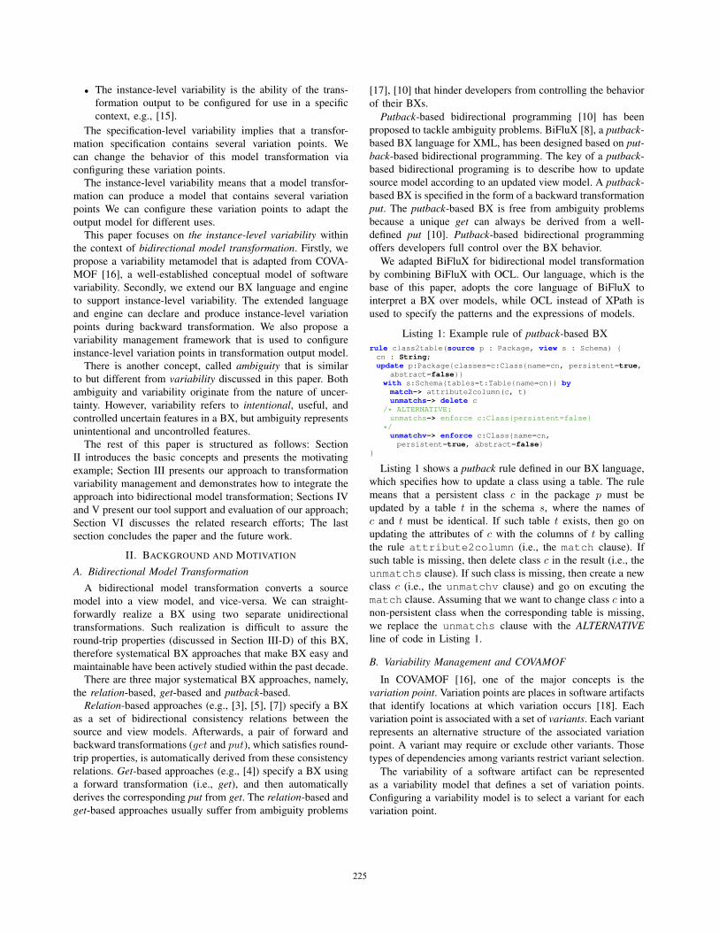
A. Overview of Our ApproachInstance-level transformation variability is the ability of the
transformation output to be configured for use in a specific
context. A (bidirectional) model transformation must can pro-
duce an output model with variation points to support instance-
level transformation variability.We identify the following requirements of transformation
variability management:
1) We must provide full control over transformation vari-
ability. Developers must can specify what types of
variation points and variants exist. Take UMLtoRDBMSas an example. If developers regard variant 2 in Fig. 1
unnecessary, then they must can exclude this variant.
2) We must provide the support for managing dependencies
among variation points and variants. As demonstrated in
Section II-C, a variant may depend on other variants.
Such dependency must can be specified, established,
stored and validated.
This section proposes our instance-level transformation vari-
ability approach that fulfills the above two requirements. Fig.
3 shows the overview of our approach that comprises the
following three major steps:
1) Developers define a variability-aware BX using our BX
language.
2) The variability-aware BX is performed on our
variability-aware BX engine. This engine captures vari-
ation points at runtime, and then produces an interme-
diate transformation output associated with a variabil-
ity model. This transformation output is intermediate
226
Technical Contributions of This Paper
Transformation Engine
Variability Management Framework
supporting the instance-level variability
an intermediate output and a variability model
the input model(s) supporting variability management
final output model(s)
a variability-aware BX specification
developers define a variability-aware BX specification
the engine interprets the BX and generates a result
with variation points
the user of transformation output configures the variability model and derives a final output using our variability management framework
1. A variability metamodel and a variability management framework for BX
2. A variability-aware BX language and a supporting engine
Fig. 3: Overview of our approach
because it contains variation points that are externally
stored in the associated variability model as first-class
elements. Developers turn the intermediate output into
a final output after configuring all variation points.
3) The variability model (as well as the intermediate out-
put) is loaded into our variability management frame-
work. Afterwards, the user of the transformation output
creates a configuration by selecting variants existing in
the variability model. Lastly, the framework derives the
final transformation output from the intermediate output
according to this configuration.
Specifically, we propose 1) a variability metamodel and a
management framework that are used to declare and configure
variability models respectively, and 2) a variability-aware BX
language and its engine, as a prototype implementation and a
demonstration of integrating variability into BX.
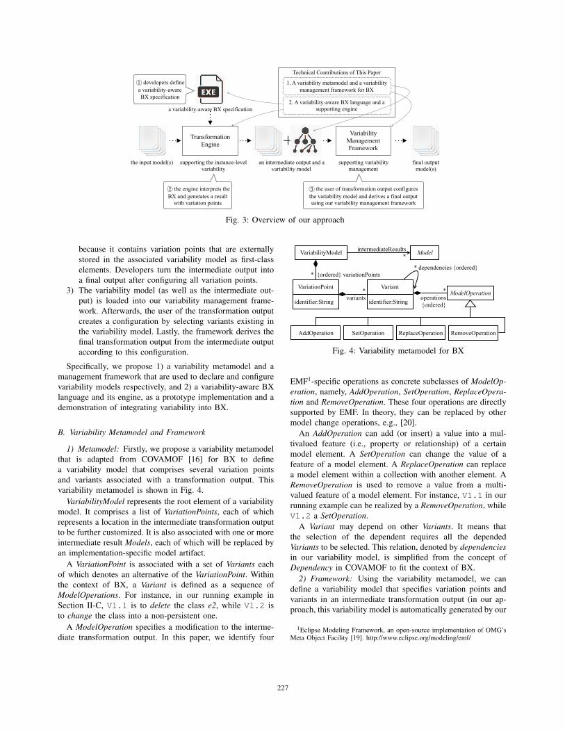
B. Variability Metamodel and Framework
1) Metamodel: Firstly, we propose a variability metamodel
that is adapted from COVAMOF [16] for BX to define
a variability model that comprises several variation points
and variants associated with a transformation output. This
variability metamodel is shown in Fig. 4.
VariabilityModel represents the root element of a variability
model. It comprises a list of VariationPoints, each of which
represents a location in the intermediate transformation output
to be further customized. It is also associated with one or more
intermediate result Models, each of which will be replaced by
an implementation-specific model artifact.
A VariationPoint is associated with a set of Variants each
of which denotes an alternative of the VariationPoint. Within
the context of BX, a Variant is defined as a sequence of
ModelOperations. For instance, in our running example in
Section II-C, V1.1 is to delete the class e2, while V1.2 is
to change the class into a non-persistent one.
A ModelOperation specifies a modification to the interme-
diate transformation output. In this paper, we identify four
ModelOperation
* {ordered} variationPoints
* operations {ordered}
* dependencies {ordered}
AddOperation SetOperation ReplaceOperation RemoveOperation
VariabilityModel
VariationPoint
identifier:String
Variant
identifier:String
ModelintermediateResults *
*variants
Fig. 4: Variability metamodel for BX
EMF1-specific operations as concrete subclasses of ModelOp-eration, namely, AddOperation, SetOperation, ReplaceOpera-tion and RemoveOperation. These four operations are directly
supported by EMF. In theory, they can be replaced by other
model change operations, e.g., [20].
An AddOperation can add (or insert) a value into a mul-
tivalued feature (i.e., property or relationship) of a certain
model element. A SetOperation can change the value of a
feature of a model element. A ReplaceOperation can replace
a model element within a collection with another element. A
RemoveOperation is used to remove a value from a multi-
valued feature of a model element. For instance, V1.1 in our
running example can be realized by a RemoveOperation, while
V1.2 a SetOperation.
A Variant may depend on other Variants. It means that
the selection of the dependent requires all the depended
Variants to be selected. This relation, denoted by dependenciesin our variability model, is simplified from the concept of
Dependency in COVAMOF to fit the context of BX.
2) Framework: Using the variability metamodel, we can
define a variability model that specifies variation points and
variants in an intermediate transformation output (in our ap-
proach, this variability model is automatically generated by our
1Eclipse Modeling Framework, an open-source implementation of OMG’sMeta Object Facility [19]. http://www.eclipse.org/modeling/emf/
227

engine). We present a transformation variability management
framework to manage this variability model.
Our variability management framework has the following
major functions: Firstly, it provides a configuration editor to
users to configure a variability model that complies with the
variability metamodel; Secondly, it can validate the configura-
tion of the variability model; Thirdly, it can interpret a valid
configuration and convert a intermediate output model into a
final output that does not contain variation points.
Configuring a variability model is to select variants for
all variation points. For a configuration that comprises a set
of Variants selected, our variability management framework
can determine whether this configuration is valid using the
following validation rules:
Rule 1: For each VariationPoint vp, only one of its Variantscan be selected, i.e.,
∀vp(v1, v2 ∈ vp.variants ∧ v1, v2 are selected ⇒ v1 = v2)
For instance, in our running example, V1.1 or V1.2 can be
selected, but they cannot be selected meanwhile.
Rule 2: If Variant v is selected, then all Variants v depends
on must also be selected because v requires all of them, i.e.,
∀v(v is selected ⇒ ∀v′(v′ ∈ v.dependencies∧v′ is selected))
For example, if V4.2 is selected, V1.2 and V2.2 must also
be selected.
Rule 3: For each VariationPoint vp, at least one of its
associated Variants that are selectable must be selected, i.e.,
∀vp(S(vp) �= ∅ ⇒ ∃v(v ∈ S(vp) ∧ v is selected))
where S(vp) ≡ {v|v ∈ vp.variants∧ isSelectable(v)}. This
rule means that all VariationPoints must be configured.
The function isSelectable determines whether a Variant can
be selected. Variant v is selectable iff none of its sibling Vari-ants is selected and all Variants v depends on are selectable.
isSelectable(v) is defined as follows:
∀v′(v, v′ ∈ vp.variants ∧ v′ �= v ⇒ v′ is not selected)∧∀v′′(v′′ ∈ v.dependencies ⇒ isSelectable(v′′) = true)
When a configuration of a variability model is valid, our
framework can interpret it by applying all ModelOperationsthat are associated with the selected Variants in this configu-
ration to the intermediate output in a proper order to derive a
final output model.
We define a partial order ≺ to determine the execution order
of two ModelOperations. o1 ≺ o2 means that o1 must be
executed before o2. Assuming that two ModelOperations o1and o2 are associated with two Variants v1 and v2 respectively,
≺ is defined as follows:
• If v1 = v2 = v and v.operations.indexOf(o1) <v.operations.indexOf(o2), then o1 ≺ o2.
• If v1 ∈ v2.dependencies, then o1 ≺ o2. Specifically, if
v2 depends on v1, all operations associated with v1 must
be performed before the operations associated with v2.
• Provided that v1 ∈ vp1.variants, v2 ∈ vp2.variantsand VariationPoints vp1 and vp2 belong to Variability-Model vm, if vm.variationPoints.indexOf(vp1) >vm.variationPoints.indexOf(vp2), then o1 ≺ o2.
With the help of ≺, our framework interprets a configuration
according to Algorithm 1.
Algorithm 1: Interpreting a configuration
Input: conf , a valid configuration; mI , a intermediate
transformation output model
Output: mF , a final output model
1 V = {all Variants selected in conf};
2 O =⋃
vi∈V
{o|o is a ModelOperation associated with vi};
3 sort O using the order ≺;
4 mF = apply all ModelOperations in O successively to
mI ;
5 return mF ;
C. Variability-Aware BX
We must extend a BX language and its execution engine
for specifying and performing variability-aware BXs. We use
our putback-based BX language and its engine introduced
in Section II to demonstrate how to integrate instance-level
variability into model transformation. We assume that the sameidea can also be applied to other transformation languages.
1) Language: We proposes the following new types of
statements to specify the instance-level variability, i.e., the
variable and maybe statements:
variable [identifier] {statement+ }maybe [identifier] (when [identifier]+)? statement
A variable statement declares a scope with variability.
Each execution of this statement will result in a VariationPointin the intermediate output. A variable statement has an
identifier expression, which is used to uniquely identify
a VariationPoint in a variability model.
A variable statement comprises several maybe state-
ments each of which declares a Variant. A maybe statement
also has an identifier expression, which is used to
uniquely identify a Variant within a VariationPoint created
from the variable statement that contains this maybestatement. A maybe statement may own a when clause to
specify what Variants this maybe statement depends on by
using a list of identifiers.
Within a variable statement, all the model modification
statements must be placed under a certain maybe statement.
Thereby, our transformation engine can capture all the changes
to the result model, and can record them in the Variant element
created by the maybe statement.
Listing 2: Examples of variability declaration
variable[’table deletion’+c] {maybe[’delete’] delete c;maybe[’keep’] enforce c:Class{persistent=false}
}
228

variable[’super’+c+p] {maybe[’remove’] when[’table deletion’+c+’keep’]delete c.super=p;
maybe[’preserve’] when[’table deletion’+c+’keep’] {}}
Listing 2 shows two variable statements. The first
variable statement (lines 1 to 4) declares that how to
propagate the deletion of a table to class c is a variation point
(e.g., VP1 and VP2 in our running example). It comprises
two maybe statements that denote two variants, i.e., deleting
c (e.g., V1.1 and V2.1) and changing c into a non-persistent
one (e.g., V1.2 and V2.2). Given that we must associate a
variation point that is created by this variable statement
with class c, the identifier expression of this variablestatement is a concatenation of string “table deletion” and c.We can replace the delete statement in line 7 of Listing
1 (i.e., the unmatchs statement) with the first variablestatement in Listing 2 to integrate this variability into the BX.
Thereby, when a table is deleted, a VariationPoint will be
created for the class corresponding to this table by executing
this variable statement.
The second variable statement (lines 5 to 9) in Listing
2 declares a variation point about how to update the super-
relationship between classes p and c (e.g., VP3 in our running
example), when the table corresponding to c has been deleted.
Therefore, the identifier expression of this variable state-
ment is a concatenation of string “super” and classes c and p.
This variable statement comprises two maybe statements
(lines 6 and 8) that denote two variants, i.e., deleting the
relationship (e.g., V3.1) and preserving the relationship (e.g.,
V3.2), when c is not deleted. The two maybe statements
depend on the second maybe statement in the first variablestatement (line 3). Such dependency is specified by two whenclauses, in which we combine the identifiers of the first
variable statement and its second maybe statement (i.e.,
“table deletion”+c+“keep”).
2) Execution: We extend our bidirectional model transfor-
mation engine to support the proposed variable and maybestatements. We assume that the same idea can also be applied
to other model transformation technologies.
During backward transformation, variable and maybestatements are executed to produce VariationPoints and Vari-ants. A variable statement is performed based on Algo-
rithm 2. Briefly, our engine creates a VariationPoint vp and
pushes vp onto a stack of VariationPoints. Afterwards, the
inner statements of the variable statement being executed
(including all maybe statements) are executed.
A maybe statement is executed based on Algorithm 3.
Firstly, our engine calculates the required Variants (lines 1 to
7) according to the when clause of the maybe statement being
executed. If any required Variant is missing, then the engine
will skip this maybe statement (line 4 and 5). Secondly, our
engine creates and initialize a new Variant v (lines 8 to 13).
Thirdly, our engine performs all ModelOperations that belong
to the Variants recursively depended by v (lines 16 to 18).
Afterwards, our engine executes all statements contained in
this maybe statement and captures all model changes that
Algorithm 2: executeVariableStatement(vs)
Input: vs, the variable statement to be executed
1 vp = new VariationPoint;
2 variationPointStack.push(vp);3 foreach statement s included by vs do4 execute s;
5 variationPointStack.pop();
Algorithm 3: executeMaybeStatement(vs)
Input: ms, the maybe statement to be executed
1 dvs = ∅;
2 foreach identifier expression vi in when clause of vs do3 dv = the Variant, previously created, whose identifier
is equal to the value of vi;4 if dv is null then5 return ; // skip this maybe statement6 else7 dvs.add(dv);
8 v = new Variant;
9 v.identifier = the value of the identifier expression
belonging to ms;
10 rvs ={x|x ∈ dvs∨∃y(y ∈ rvs∧x ∈ y.dependencies
)};
11 v.dependencies = dvs ∪ {variantStack.top()};
12 vp = variationPointState.top();13 vp.variants.add(v);14 copy current runtime state;
15 variantStack.push(v);16 ops =
⋃
x∈rvsx.operations;
17 sort ops using the partial order ≺;
18 execute all ModelOperations in ops;
19 foreach statement s included by ms do20 execute s and record all ModelOperations when s is
being executed;
21 v.operations = {all recorded ModelOperations};
22 undo all ModelOperations in v.operations and ops;
23 variantStack.pop();24 restore runtime state;
25 return;
happen during the execution of the inner statements (lines 19
to 21). Lastly, our engine undoes all ModelOperations in the
reversed order and restores the runtime state (lines 22 to 24).
Take the first variable statement in Listing 2 as an
example. When this variable statement is executed, its two
maybe statements are executed successively. When the first
maybe statement is executed, the class bound to c is deleted,
and our engine creates a RemoveOperation for this change.
Afterwards, the runtime state is restored, and then the second
maybe statement is executed, resulting a new Variant with
a SetOperation that changes the class bound to c into a non-
persistent class. Finally, the runtime state is restored again and
229

a VariationPoint with two Variants is produced.
During forward transformation, executing variable and
maybe statements will cause a runtime exception because our
approach does not support variability of forward transforma-
tion. Not supporting variability in the forward transformation
can make it easier for developers to define a correct BX.
It is worthwhile to notice that in our approach, a variability-
aware BX is still executed in a deterministic way, despite that
it produces an output model with variation points.
D. Round-trip Property of BX with Variability
The most important BX properties are round-trip properties,
i.e., the GetPut and PutGet laws. Without variability, round-
trip properties are defined [10] as follows:
put(s, get(s)
)= s (GETPUT)
get(put(s, v)
)= v (PUTGET)
After integration of variability into BX, the backward trans-
formation put returns a set of candidate outputs that can be
derived from an intermediate output and a variability model.
Therefore, put with variability can be characterized as follows
(where P(S) is the power set of S):
put : S × V → P(S)
Based on the new definition of put, the round-trip properties
of a BX with variability are redefined as follows:
put(s, get(s)
)= {s} (GETPUT)
∀s′(s′ ∈ put(s, v) ⇒ get(s′) = v)
(PUTGET)
The GetPut law says that the result of the backward trans-
formation carried out immediately after the forward transfor-
mation should be equal to the original source model. The
PutGet law says that for any candidate final result s′ obtained
by transforming a view model v in the backward direction,
the result of converting s′ in the forward direction should be
equal to v. Currently, the developers must assure the round-trip
property of the BX they defined. How to verify the round-trip
property automatically is our future work.
IV. TOOL SUPPORT
We have implemented a tool2 support to BX variability,
including our extended BX engine and a variability manage-
ment tool. Fig. 5 presents a screenshot of our BX editor and
variability management tool.
Fig. 5: Screenshot of tool support
2Source code is available at https://bitbucket.org/ustbmde/morel/wiki/Home
V. EVALUATION
The objective of this section is to evaluate the feasibilityand the performance of the proposed approach. The objective
is further refined by the following two research questions:
RQ1: Can the proposed approach be used to handle theinstance-level variability in BXs, which come from differentapplication domains? RQ2: What is the performance lossincurred by the proposed approach, compared with the BXswithout variability? To answer RQ1, we make two variability-
aware BXs having variability to demonstrate the feasibility of
our approach. With regard to RQ2, we conduct an experiment
in performance that compares these variability-aware BXs with
corresponding BXs without variability, respectively.
A. UML to RDBMS
The first BX is UMLtoRDBMS, our running example. This
BX is intended to demonstrate that our approach can support
complex variant points and dependencies. We identify four
types of variation points in total.
The first two types of variation points are about how to
propagate the deletion of a table and how to update the
super-relationships among classes. Given that they have been
presented in Listing 2 and explained in Section III-C, this
section omits their details.
The third type of variation points is about converting a
column of a table back to an attribute of a class. Given a
column cl in a table t and a class c corresponding to t, assume
that we cannot find an attribute in class c that corresponds to
cl. To convert cl, we must determine whether cl can match
any attribute inherited from any superclass of c. Due to the
influence of the first two types of variation points, we have
several possible strategies of converting cl as follows: starting
from each direct superclass sc of c,
• if sc is a persistent class and contains an attribute which
matches cl, then return (this is the default update strategy
rather than a Variant);• if sc is or is changed into a non-persistent class and the
inheritance from c to sc is preserved, go on searching in
superclasses of sc;• otherwise, stop searching, and then create a new attribute
that matches cl in c.
The last two cases can be specified as Listing 3. Lines 2 and 3
specify the second case, and lines 4 and 5 the third case. Notice
that in Listing 3, we specify dependencies among Variantsusing when clauses.
Listing 3: Variation point of updating super attributes
variable[’update super attribute’+c+sc+cl.name] {maybe[’go on’] when[’super’+c+sc+’keep’]... /* go on searching in the superclasses of sc */
maybe[’stop’] when[’super’+c+sc+’delete’]enforce c:Class{attributes=a:Attribute{name=cl.name}}
}
The fourth type of variation points is about how to propagate
the deletion of a foreign key back to an association in Class
Diagram. In UMLtoRDBMS, a foreign key fk, which connects
two tables, is transformed from an association assoc, which
230

<<class>> <<non-persistent>>
e2a2
<<class>> e2
<<table>> e1’
a1 e2-a2 e2-e3-a3
<<table>> e2’
a2 e3-a3
<<table>> e3’
a3
a1 e2-a2
a2 a3l1 l2
DEL
VP1 VP4VP2 VP3
V1.1
V1.2
V4.1
V4.2
V2.1
V2.2
V3.1
V3.2
delete
keep
delete
keep
delete
keep
delete
keep
put
RDBMS Model (view model)
Class Diagram (intermediate output)
Variability Model
r1
e3-r1-e2:foreignKeyDEL
VP5
V5.1
V5.2
go on
stop
VP6
V6.1
V6.2
go on
stop
output 1
output 2
output 3
Class Diagram (final outputs)
V1.2, V2.2, V3.2, V4.2, V5.1, V6.1
V1.2, V2.2, V3.1, V4.2, V5.1, V6.2
V1.2, V2.1, V3.2, V4.1, V5.2
Configuration (selected variants)
<<class>> e1
<<class>> e3
<<class>> e1
<<class>> e3
a1 e2-a2
a3r1
l1 l2
<<class>> <<non-persistent>>
e2
<<class>> e1
<<class>> e3
a2a3
r1
l1 l2
a1 e2-a2 e2-e3-a3
<<class>> e1
<<class>> e3
a3
l2
a1 e2-a2 e2-e3-a3
<<class>> <<non-persistent>>
e2a2
Fig. 6: Example of UMLtoRDBMS
connects two classes. If only fk is deleted while the associated
tables are preserved, then delete assoc. If fk and at least
one of the associated tables (e.g., t) are deleted, there are
two variants as follows: 1) delete assoc; 2) when the class tcthat corresponds to t is changed into a non-persistent class,
then preserve assoc because this BX does not convert any
information related to non-persistent classes, as mentioned in
Section II-C. The two variants are encoded as Listing 4:
Listing 4: Variation point of updating associations
variable[’deletion of foreign key’+sc+tc+an] {maybe[’delete’] delete assoc;maybe[’keep’] when[’table deletion’+tc+’keep’] {}
}
Fig. 6 shows an example that contains all types of variation
points. In the original source model, there are three classes,
namely, e1 to e3, and an association r1 from e3 to e2. e1,
e2 and e3 have three attributes a1, a2 and a3, respectively.
Besides, e1 inherits from e2, and e2 inherits from e3. The
original source model results in a view model that contains
three tables and a foreign key (called e3-r1-e2).
Assume that both table e2 and foreign key e3-r1-e2 are
deleted. The backward transformation generates an intermedi-
ate output and a variability model as shown in the bottom left
part of Fig. 6. VP1, VP2 and VP3 in Fig. 6 are similar to VP1,
VP3 and VP4 in Fig. 2, respectively. VP4 denotes the variation
point about how to update r1, which is created according to
Listing 4. VP5 and VP6 denote the variation points about how
to convert column e2-e3-a3 back to an attribute in class e1,
which is created according to Listing 3.
V5.1, which depends on V2.2, represents the case that l1is preserved; V5.2, which depends on V2.1, represents the
case that l2 is deleted. V6.1, which depends on V5.1 and
V3.2, represents the case that both l1 and l2 are preserved;
V6.2, which depends on V5.1 and V3.1, represents the case
that l1 is preserved and l2 is deleted.
The middle part of Fig. 6 shows several final output models
derived from the intermediate model and the variability model,
and the rightmost part of Fig. 6 shows the corresponding
configurations. For example, result 3 is derived from V1.1,
V2.1, V3.2, V4.1 and V5.2.
B. Hierarchical Statechart to Flat StatechartThe BX between a hierarchical statechart (HSM) and a flat
statechart (FSM), which was studied by Eramo et al. [15], also
has variability. This example is used to demonstrate that our
approach can handle the BX studied by others.In brief, the forward transformation converts a HSM (i.e.,
a statechart owning composite states) into a FSM (i.e., a
statechart without composite states). A top-level state s in a
HSM will be converted into a state s’ in a FSM. A transition
that starts from or ends with a top-level state s or an inner
state of s will be converted into a transition that starts from
or ends with a state s’ in the FSM. Besides, the transitions
within a composite state will be ignored.A variability issue arises during the backward transforma-
tion when a transition is created from or to a state in a FSM
that corresponding to a composite state s owning inner states
in the HSM: s and any inner state of s can be the source or
target of tis transition in the HSM.
S1
S2
S3 S4
S5S1
S2
S5 S1
S2
S5
vt
S1
S2
S3 S4
S5
st1st2
st3get update put
Fig. 7: Example of HSMtoFSM
As shown in Fig. 7, a new transition vt is created from
S2 to S5 in the view model. In the updated source model,
the corresponding transition st can be inserted from S2, S3or S4, to S5. To handle this variability, Listing. 5 specifies
how to connect the source and target of a transition using two
variable statements. They imply that the source/target of
the transition can be the top-level state s or any of the inner
states of s obtained by iterating eAllContents of s.
231

Listing 5: Variation point declaration in HSMtoFSM
variable[’source’+vt] {maybe[’to’+s] enforce st:hsm!Transition{source=s};foreach s:hsm!CompositeState{eAllContents=inner:hsm!State{}}->maybe[’to’+inner] enforce st:hsm!Transition{source=inner}
}}variable[’target’+vt] {maybe[’to’+s] enforce st:hsm!Transition{target=s};foreach s:hsm!CompositeState{eAllContents=inner:hsm!State{}}->maybe[’to’+inner] enforce st:hsm!Transition{target=inner}
}}
The approach of Eramo et al. generates all possible final
output models automatically by using constraint solving. De-
velopers cannot design the variability of a BX, specifically,
they cannot precisely specify what particular variation points
and variants this BX has. Compared with Eramo’s approach,
our approach provide more control over BX variability without
losing the processing ability of transformation variability.
C. Performance Loss
To evaluate the impact on performance of our approach,
we compare the execution time tV of a BX having variability
with the time tD of the same BX without variability. Then,
we calculate the performance loss incurred by our approach,
which is calculated as
(tV − tD)/tD
Subject BXs. We use the two BXs (i.e., UMLtoRDBMSand HSMtoFSM) presented in Sections V-A and V-B as the
subjects to be studied. The control groups are derived from
the subject BXs, as follows: 1) for UMLtoRDBMS, a BX
(called UMLtoRDBMS-d), which always removes the class
when the table is deleted in the view model, is developed; 2)
for HSMtoFSM, a BX (called HSMtoFSM-d), which always
connects the new transition with top-level states, is developed.
Process. The experiment is conducted on a MacBook Pro
with an Intel Core i7 2.8Ghz processor and 16Gb RAM. For
each BX as well as its control group, we use a random model
generator [21] to generate an original source model. Then,
we execute the forward transformation, and obtain a view
model. After that, we create a set of modified view models,
which result in different numbers of variation points (i.e., 0,
10, 20, 30, 40, and 50 variation points). For UMLtoRDBMS,
the original source model contains 1000 model elements (i.e.,
300 classes, 600 attributes, and 100 associations). The updated
view models are created by renaming tables repeatedly. For
HSMtoFSM, the original source model also contains 1000
model elements (i.e., 100 composite states, 350 states, and
550 transitions). The updated view models are created by
renaming transitions repeatedly. Renaming an element will be
recognized by the BXs as an element insertion following a
deletion, and will not change the size of the view model.
Finally, we execute the backward transformations, including
the subject BX and its control group, and capture the average
execution times (excluding I/O).
Results. The result of case UMLtoRDBMS is shown in Fig.
8a. Since the size of the view model is constant, the execution
times of UMLtoRDBMS and UMLtoRDBMS-d did not vary a
lot. The performance loss ranged from 5.87% to 9.07%, which
Exec
utio
n Ti
me
(ms)
2500
2575
2650
2725
2800
Number of Variation Points0 10 20 30 40 50
UMLtoRDBMS UMLtoRDBMS-d
6.30
% 6.21
%
5.87
% 6.90
%
9.07
%
8.97
%
(tV ) (tD)
(a) Result of UMLtoRDBMS
Exec
utio
n Ti
me
(ms)
450
562.5
675
787.5
900
Number of Variation Points0 10 20 30 40 50
HSM2FSM HSM2FSM-d
8.88
% 20.6
4%
32.2
7% 45.0
3%
59.8
4%
61.8
1%
(tV ) (tD)
(b) Result of HSMtoFSM
Fig. 8: Results of experiment in performance loss
is acceptable. The result of case HSMtoFSM is shown in Fig.
8b. The execution times of HSMtoFSM-d increased slightly.
However, the execution times of HSMtoFSM increased linearly
with the number of variation points, and the performance
loss increased (almost linearly) from 8.88% to 61.81%. It is
because HSMtoFSM has to traverse all the inner states of top-
level composite states, while HSMtoFSM-d does not. Hence,
the more variation points there are, the more inner states
HSMtoFSM visited, and consequently, the more performance
loss is incurred. Overall, this experiment shows that the
performance loss incurred by our approach is reasonable.
D. Threats to Validity
The first threat to validity is the choice of the two example
BXs studied, which are relatively simple. However, they are
sufficient to demonstrate the feasibility and the usage of our
approach. The second threat to validity is the complexity of
the test input models. In the future, we plan to conduct more
experiments to validate the scalability of our approach to
mitigate this threat.
VI. RELATED WORK
Variability management in model transformation has been
discussed from both the theoretical and the solution aspect.
From the theoretical aspect, Stevens [17] analyzed the uncer-
tainty issue, which may result in variability in practice, in
the context of bidirectional transformation; Diskin et al. [22]
proposed a formal framework of delta-lens supporting uncer-
tainty. They both can be used as a guide to the development
of concrete solutions.
Concrete solutions to variability management in (bidirec-
tional) model transformation can be roughly divided into
two groups: the specification-level and the instance-level,
232

as discussed in Section I. Struber et al. [14] proposed a
specification-level approach to variability-based model trans-
formation. Their approach enables developers to define a
model transformation containing variation points. Given a
valid configuration, a classical transformation that has no
variation point can be derived. To facilitate defining variability-
based transformations, they also proposed a rule merging
algorithm [13]. Salay et al. [23] also proposed an approach
that lifts model transformation to product lines. However, their
approach is designed for the variability in input models.
As for the instance-level solutions, Eramo et al. [15] pro-
posed a metamodel-based approach. The basic idea of their
approach is to automatically derive an uncertainty metamodel
from the metamodel used by a BX. Afterwards, they encode
this BX and uncertainty metamodel into a constraint solving
problem. Therefore, a constraint solver can find all models
each of which conforms to the uncertainty metamodel and
represents a variant output of the BX. However, they did not
discuss how to support dependencies among variants. The
constraint-solving-based BX approach, proposed by Macedo
et al. [7], also has the potential to support the instance-
level variability by asking the solver to find all possible
result models. However, this kind of approach may not be
scalable when there are a lot of variation points. Our approach,
which is also an instance-level approach, differs from the
above approaches. Instead of asking a solver to explore the
search space freely, our approach provides developers with
full control over their BXs. Developers can explicitly specify
what types of variation points, variants and dependencies may
exist in the BX output, and how to produce them.
VII. CONCLUSION AND FUTURE WORK
The major contributions of this paper are summarized as fol-
lows: 1) a variability metamodel and management framework
for model transformation; 2) a BX language and an engine as
a demonstration to support the definition and execution of a
BX with variability; 3) two examples of BXs with variability
that illustrated the feasibility of the proposed approach.
In the future, we plan to explore how to use our approach
to support the specification-level variability. Besides, during
our evaluation, we observed that many human efforts were
required to configure the variability model when there were
a number of variation points. Although our tool support can
check, filter and highlight available variants to ease the config-
uration, we assume that more the usability of our tool can be
further enhanced. Lastly, more case studies and experiments
will be conducted to evaluate our approach.
ACKNOWLEDGEMENT
This work was supported by the National Natural Science
Foundation of China (61300009, 61472180).
REFERENCES
[1] Z. Diskin, “Algebraic models for bidirectional model synchronization,”in Model Driven Engineering Languages and Systems. Springer, 2008,pp. 21–36.
[2] H. Giese and R. Wagner, “From model transformation to incrementalbidirectional model synchronization,” Software & Systems Modeling,vol. 8, no. 1, pp. 21–43, 2009.
[3] H. Song, G. Huang, F. Chauvel, Y. Xiong, Z. Hu, Y. Sun, andH. Mei, “Supporting runtime software architecture: A bidirectional-transformation-based approach,” Journal of Systems and Software,vol. 84, no. 5, pp. 711–723, 2011.
[4] Y. Xiong, H. Song, Z. Hu, and M. Takeichi, “Synchronizing concur-rent model updates based on bidirectional transformation,” Software &Systems Modeling, vol. 12, no. 1, pp. 89–104, 2013.
[5] A. Cicchetti, D. Di Ruscio, R. Eramo, and A. Pierantonio, “JTL:a bidirectional and change propagating transformation language,” inSoftware Language Engineering. Springer, 2010, pp. 183–202.
[6] Z. Diskin, Y. Xiong, K. Czarnecki, H. Ehrig, F. Hermann, and F. Orejas,“From state-to delta-based bidirectional model transformations: Thesymmetric case,” in Model Driven Engineering Languages and Systems.Springer, 2011, pp. 304–318.
[7] N. Macedo and A. Cunha, “Implementing qvt-r bidirectional modeltransformations using alloy,” in Fundamental Approaches to SoftwareEngineering. Springer, 2013, pp. 297–311.
[8] H. Pacheco, T. Zan, and Z. Hu, “Biflux: A bidirectional functional updatelanguage for xml,” in Proceedings of the 16th International Symposiumon Principles and Practice of Declarative Programming. ACM, 2014,pp. 147–158.
[9] S. Hidaka, M. Tisi, J. Cabot, and Z. Hu, “Feature-based classification ofbidirectional transformation approaches,” Software & Systems Modeling,pp. 1–22, 2015.
[10] S. Fischer, Z. Hu, and H. Pacheco, “The essence of bidirectionalprogramming,” Science China Information Sciences, vol. 58, no. 5, pp.1–21, 2015.
[11] OMG, “Meta Object Facility (MOF) 2.0 Query/View/Transformationspecification v1.2,” Object Management Group, Tech. Rep. formal/15-02-01, 2015.
[12] J. Van Gurp, J. Bosch, and M. Svahnberg, “On the notion of variabilityin software product lines,” in Proceedings 2001 Working IEEE/IFIPConference on Software Architecture. IEEE, 2001, pp. 45–54.
[13] D. Struber, J. Rubin, T. Arendt, M. Chechik, G. Taentzer, and J. Ploger,RuleMerger: Automatic Construction of Variability-Based Model Trans-formation Rules. Berlin, Heidelberg: Springer Berlin Heidelberg, 2016,pp. 122–140.
[14] D. Struber, J. Rubin, M. Chechik, and G. Taentzer, “A variability-based approach to reusable and efficient model transformations,” inFundamental Approaches to Software Engineering. Springer, 2015,pp. 283–298.
[15] R. Eramo, A. Pierantonio, and G. Rosa, “Managing uncertainty inbidirectional model transformations,” in Proceedings of the 2015 ACMSIGPLAN International Conference on Software Language Engineering.ACM, 2015, pp. 49–58.
[16] M. Sinnema, S. Deelstra, J. Nijhuis, and J. Bosch, “COVAMOF: Aframework for modeling variability in software product families,” inSoftware product lines. Springer, 2004, pp. 197–213.
[17] P. Stevens, “Bidirectional model transformations in QVT: semanticissues and open questions,” Software & Systems Modeling, vol. 9, no. 1,pp. 7–20, 2010.
[18] I. Jacobson, M. Griss, and P. Jonsson, Software reuse: architecture,process and organization for business success. ACM Press/Addison-Wesley Publishing Co., 1997.
[19] Object Management Group, OMG Meta Object Facility (MOF)Core Specification Version 2.4.1, 2011. [Online]. Available: http://www.omg.org/spec/MOF/2.4.1
[20] I. Rath, G. Varro, and D. Varro, Change-Driven Model Transformations.Berlin, Heidelberg: Springer Berlin Heidelberg, 2009, pp. 342–356.
[21] X. He, T. Zhang, C.-J. Hu, Z. Ma, and W. Shao, “An mde performancetesting framework based on random model generation,” Journal ofSystems and Software, 2016.
[22] Z. Diskin, R. Eramo, A. Pierantonio, and K. Czarnecki, “Incorporatinguncertainty into bidirectional model transformations and their delta-lensformalization,” in Proceedings of the Fifth International Workshop onBidirectional Transformations (Bx 2016), Eindhoven, The Netherlands,April 8, 2016 2016.
[23] R. Salay, M. Famelis, J. Rubin, A. Di Sandro, and M. Chechik, “Liftingmodel transformations to product lines,” in Proceedings of the 36thInternational Conference on Software Engineering. ACM, 2014, pp.117–128.
233


