

Civil Engineering Infrastructures Journal, 48(1): 133-156, June 2015
ISSN: 2322-2093
133
Two New Quadrilateral Elements Based on Strain States
Rezaiee-Pajand, M.1*
and Yaghoobi, M.2
1 Professor, Civil Engineering Department, Ferdowsi University of Mashhad, Mashhad, Iran 2
Ph.D. Candidate, Civil Engineering Department, Ferdowsi University of Mashhad,
Mashhad, Iran
Received: 28 Dec. 2013 Revised: 28 Apr. 2014 Accepted: 30 Apr. 2014
Abstract: In this paper, two new quadrilateral elements are formulated to solve plane problems. Low sensitivity to geometric distortion, no parasitic shear error, rotational invariance, and satisfying the Felippa pure bending test are characteristics of these suggested elements. One proposed element is formulated by establishing equilibrium equations for the second-order strain field. The other suggested element is obtained by establishing equilibrium equations only for the linear part of the strain field. The number of the strain states decreases when the conditions among strain states are satisfied. Several numerical tests are used to demonstrate the performance of the proposed elements. Famous elements, which were suggested by other researchers, are used as a means of comparison. It is shown that these novel elements pass the strong patch tests, even for extremely poor meshes, and one of them has an excellent accuracy and fast convergence in other complicated problems.
Keywords: Equilibrium Conditions, Optimization Criteria, Plane Problems, Quadrilateral Elements, Strain States
INTRODUCTION
Free formulation was first based on
kinematics decomposition. Free
formulation indicates that the basic part
fulfills convergence of the finite element.
Felippa (2006) set up the correct rank of
the stiffness matrix and increased accuracy
using the high-order part. Strain gradient
notation creates a suitable space to find the
error of the finite element pattern using a
Taylor series expansion of the strain field.
This scheme adequately specifies shear
locking and parasitic shear error. In other
words, the slopes of the strains point to the
root of many finite element modeling
errors (Dow, 1999).
The parameterized variational principle
in the formulation of finite element
technique changed the science of high-
performance elements. In this way,
Corresponding author Email: [email protected]
scientists could define the continuous
space of an elastic functional. Making the
continuous space of the functional
stationary produces free parameters for
formulation of the element, creating finite
element templates (Felippa and Militello,
1990). Further investigation revealed that
the template formulations followed
specific and identical structures. There was
no need to make the parametrized
functional stationary to obtain these
templates. Assigning values to the free
parameters of these templates provides the
various elements (Felippa, 2000).
Optimization of finite element templates is
difficult, however, and requires innovation.
The large number of free parameters,
symbolic processing and matrix structure
optimization are difficulties faced by
researchers who study the templates.
Strain gradient notation is a simple and
clear demonstration of free formulation.
An efficient element of SSQUAD (strain
Rezaiee-Pajand, M. and Yaghoobi, M.
134
state quadrilateral element) was recently
proposed using strain gradient notation and
free formulation (Rezaiee-Pajand and
Yaghoobi, 2012). In this element, the
optimization constraints of insensitivity to
distortion, rotational invariance and
absence of parasitic shear error were
employed. It was evident that a complete
selection of strain states from each order
satisfies all three conditions. In addition,
the need to establish an optimization
constraint for bending in the linear strain
states was identified in the formulation.
Entering the states of rigid body motion is
a convergence criterion of the formulation.
To fulfill this condition, a linear strain
field is used for the SSQUAD element.
Equilibrium allowed establishment of
equations among the strain states.
Consequently, two strain states could be
written in terms of other strain states. This
decreased the number of the strain states
required in the formulation. Equilibrium
equations for formulation of the SSQUAD
element increased the performance of the
element. It should be noted that hybrid
stress elements satisfy equilibrium
conditions in a strong form (Santos and
Moitinho de Almeida, 2014(. As will be
demonstrated, completely satisfying the
equilibrium equation does not produce
more accurate responses. In fact, using the
rotational degree of freedoms and
satisfying equilibrium in second-order
filed decrease the ability of the suggested
element. To eliminate this weakness,
equilibrium should be satisfied in the
linear displacement field.
Severe numerical tests display fast
convergence and insensitivity to distortion
in the mesh for the SSQUAD element.
This element, like other good elements,
such as AGQ6-II, provides answers with
large error in strong patch tests for
constant stress and bending with bilinear
stress for high distortion (Prathap and
Senthilkumar, 2008).
The present study uses high-order fields
and imperfectly establishes equilibrium
equations to eliminate the weakness of the
SSQUAD element in the strong patch tests
of constant stress and bending with bilinear
stress for high distortion. Selecting a
complete second-order strain field satisfies
optimization constraints for insensitivity to
geometric distortion, absence of parasitic
shear error, and rotational invariance. The
new element also satisfies Felippa's pure
bending test. To apply a second-order strain
field, 20 strain states are needed to present
the element.
Satisfying the equilibrium equations is
explored using perfect and imperfect types.
The SSQ14 element (strain state
quadrilateral element with 14 DOF) is
obtained by setting up perfect equilibrium
equations for the second-order strain field.
The SSQ18 element (strain state
quadrilateral element with 18 DOF) is
obtained by employing equilibrium
equations only for the linear part of the
strain field. Relationships among the strain
states are created using equilibrium
equations. In the new formulation, these
equations decreases the number of required
strain states for SSQ14 and SSQ18 to 14
and 18, respectively.
The proposed formulations are based on
Taylor's expansion of the strain field.
Several optimal constraints are included to
obtain errorless responses. The equilibrium
conditions are satisfied, to some extent,
using only the constant parts of the strains.
The proposed strategy provides two simple
elements that pass the patch test and work
efficiently, even in coarse distorted meshes.
These types of elements are innovative,
and their performance is examined using a
variety of numerical tests. The responses to
high-quality elements of other researchers
are also used as a means of comparison.
Section 4.1 explains the improved
performance of SSQ18 and SSQ14 elements
over other good elements, such as SSQUAD
and AGQ6-II. The SSQ18 element also
demonstrates superior accuracy and fast
convergence in other tests.
Civil Engineering Infrastructures Journal, 48(1): 133-156, June 2015
135
Optimization Constraints
A formulation that allows optimization
is required to obtain efficient elements.
The proposed strategy demonstrates the
roots of many errors. Sufficient constraints
must be a component of any formulation to
improve performance. The following
subsections explain the constraints used in
the proposed technique.
In-plane pure bending test
Felippa used this test to find the
optimum bending template (Felippa, 2003,
2004, 2006). He examined the responses of
the template for in-plane bending by
evaluating the energy ratios using an
Euler-Bernoulli beam where xr and yr
denote the bending energy ratios of a
rectangular part of the beam in the x and y
directions, respectively. If rx = 1, ry = 1, or
r = 1, the element can model flexure in an
arbitrary direction. If r > 1 or r < 1, the
element is either over-stiff or over-flexible.
For each aspect ratio of element r = 1, the
element is at flexural optimum. In the case
of insensitivity to the aspect ratio, r
increases, and the element will experience
shear locking.
When this test is based on strain states
and in-plane bending occurs in the x
direction, the real stress field changes
linearly in the y direction. The strain field
for this case is based on the Hooke's law as
follows:
0 γ,y ,y xy43y21x (1)
where 1 , 2 , 3 and 4 : are constant
coefficients and Eq. (1) shows that only
)( yy,ε , )( yx,ε , )( yε and )( xε strain states
exist in this field. For bending in the y
direction, the real strain field includes
)( xy,ε , )( xx,ε , )( yε and )( xε strain states.
To obtain the real answer for in-plane
bending, )( yy,ε , )( xy,ε , )( yx,ε , )( xx,ε ,
)( yε and )( xε strain states must be used.
)( xε : is the magnitude of axial strain xε at
the origin, )( x,xε , and )( yx,ε are the rate
of xε variations in x and y directions, in
the vicinity of origin, respectively. Other
coefficients are also determined by using a
similar tactic.
The existence of constant strain states
and rigid body motions in the assumed
strain field of the element is a convergence
criterion and must exist in all cases. The
bending test based on strain states has no
limitation for geometric shape or type of
mesh. It covers elements other than the
triangular and quadrilateral elements.
Rotational invariance
The properties of some elements change
if the coordinate axes rotate. These
elements are not rotational invariant. An
element having different rotated shapes in
the mesh of the structure inevitably
requires rotational invariance. Rotational
invariance depends on the complete
selection of expressions of the strain field
of each order (Dow, 1999).
Absence of parasitic shear error
The appearance of axial strain states in
shear strain interpolation polynomial
creates parasitic shear error, which leads to
hardening of the element (Dow, 1999).
Shear strains, including Taylor series shear
strain, are independent of axial strain. In
the shear strain interpolation function of
elements with parasitic shear error, some
axial strain states incorrectly appear. If
such an element experiences flexural
deformation, the axial strain states are non-
zero and are erroneously representative of
part of the shear strain. In elements
formulated using strain gradient notation,
the parasitic shear error can be eliminated
by setting aside the spurious strain states
from the shear strain polynomial. Parasitic
shear error decreases as the mesh becomes
finer. Despite this, if an element is free of
error, coarse mesh will also produce
correct answers. It should be noted that the
Rezaiee-Pajand, M. and Yaghoobi, M.
136
selection of the complete strain
interpolation functions prevents the
appearance of this error.
Equilibrium conditions
In formulation of the SSQUAD
element, setting up the equilibrium
equations increases the performance of the
element and decreases the number of strain
states. By selecting a complete polynomial
from each order, inclusion of parasitic
shear and the rotational variance errors can
be prevented.
The linear strain field was used to
formulate the SSQUAD element. SSQ14
and SSQ18 were formulated using a
complete second-order strain field. By
selecting this field, rotational invariance
and absence of parasitic shear error are
guaranteed. It is evident that this field can
satisfy the Felippa pure bending test. The
difference between SSQ14 and SSQ18 is
in the establishment of equilibrium
equations. In the SSQ14 element, complete
equilibrium equations are set up; in the
SSQ18 element, the equilibrium equations
are satisfied for the linear part of the strain
field.
The present study shows the superiority
of the case in which the equilibrium
equations are partially fulfilled. For the
strain field of the complete second order,
20 nodal unknowns are needed. For the
full and partial establishment of the
equilibrium equations, 6 and 2 strain
states, respectively, are written in terms of
other strain states. The equilibrium
equations inside an elastic homogeneous
element for in-plane stress or strain
become:
0yx,Fy
yx,σ
x
yx,τ
0yx,Fy
yx,τ
x
yx,σ
y
yxy
x
xyx
)()()(
)()()(
(2)
where xσ , yσ and xy : are stresses at any
point on the element, and )( yx,Fx and
)( yx,Fy : are force fields inside the
element in the x and y directions,
respectively, in a Cartesian coordinate
system.
In plane problems, it is evident that the
variation of the force field in the direction
normal to the element plane (z direction
here) does not exist. The stress fields are
selected in the Cartesian coordinate
system. Based on the Hooke's law for a
homogeneous elastic state, Eq. (2) can be
written as:
)( yxxx εελ2Gεσ (3)
)( yxyy εελ2Gεσ
(4)
xyxy Gγτ
(5)
0yx,Fx
yx,γG
y
yx,ελ2G
y
yx,ελ
0yx,Fy
yx,γG
x
yx,ελ
x
yx,ελ2G
y
xy
yx
x
xy
yx
)()(
)()(
)(
)()(
)()()(
(6)
The λ for plane stress and plane strain
states are ))(( ν1ν1
νE
and
))(( 2ν1ν1
νE
,
respectively, and G, ν, and E: are elasticity
parameters of shear modulus, Poisson’s
ratio and Young’s modulus, respectively.
SSQ14 and SSQ18
The formulation of the SSQ14 and SSQ18
elements is described below based on the
assumed strain functions.
SSQ14
The formulation of SSQ14 and SSQ18
employs the strain and displacement fields
as:
Civil Engineering Infrastructures Journal, 48(1): 133-156, June 2015
137
2 2
x x x xy r x,x x,y xy,y y,x
3 2 2 3
x,xx x,xy x,yy xy,yy y,xy
2 2
y y xy r y xy,x x,y y,x y,y
u (u ) (ε ) x (γ /2 r ) y (ε ) x /2 (ε ) xy (γ ε ) y /2
(ε ) x /6 (ε ) x y/2 (ε ) y x/2 (γ ε ) y /6
u (u ) (γ /2 r ) x (ε ) y (γ ε ) x /2 (ε ) xy (ε ) y /2
(γ
3 2 2 3
xy,xx x,xy y,xx y,xy y,yyε ) x /6 (ε ) x y/2 (ε ) y x/2 (ε ) y /6
(7)
2 2
x x x,x x,y x,xx x,xy x,yy
2 2
y y y,x y,y y,xx y,xy y,yy
2
xy xy xy,x xy,y xy,xx x,yy y,xx
ε (x,y) (ε ) (ε ) x (ε ) y (ε ) x / 2 (ε ) xy (ε ) y / 2
ε (x,y) (ε ) (ε ) x (ε ) y (ε ) x / 2 (ε ) xy (ε ) y / 2
γ (x,y) (γ ) (γ ) x (γ ) y (γ ) x / 2 (ε ε )
2
xy,yyxy (γ ) y / 2
(8)
In Eq. (8), the coefficient of xy:
is )( xxy,yyx, εε . This is derived from the
strains compatibility condition, which
is )()()( xxy,yyx,xyxy, εεγ . The formulation
of SSQ14 satisfies the equilibrium
equations completely; thus, the strain field
in Equation (8) is substituted into Eq. (6).
In equilibrium equations, the body forces
of )( yx,Fx and )( yx,Fy are ignored. As a
result, the relationship among the strain
states is:
))(())(()(
))(())(()(
))(())(()(
))(())(()(
))(())(()(
))(())(()(
xxy,yyx,yyy,
yyx,xxy,xxx,
xyx,xyy,yyxy,
xyy,xyx,xxxy,
xx,xy,yxy,
yy,yx,xxy,
ελ2G
Gε
λ2G
λGε
ελ2G
Gε
λ2G
λGε
εG
λ2Gε
G
λγ
εG
λ2Gε
G
λγ
εG
λ2Gε
G
λγ
εG
λ2Gε
G
λγ
(9)
The number of unknowns in the
formulation has now decreased to 14. The
formulation is carried out using the 14
residual strain states and the vector of the
strain states is:
)()()()()()()(
)()()()()()()(
xxy,xyy,yyx,xyx,yy,xy,yx,
xx,xyyxryx
T
εεεεεεε
εγεεruuq
(10)
The displacements and strains are
transformed to the next matrix as:
q.ΝU q (11)
λ12G
yG
2
yx
6G
x λ2G
2
xyλ12G
x λG
6G
yλG
λ12G
y λG
6G
xλGλ12G
xG
2
xy
6G
yλ2G
2
yx
2G
xλ2G
2
yxy
2G
xλG
02G
yλGxy
02
xy0x10
2G
yλ2G
2
x
2
y0xy01
3232
33
33
3232
222
2
22
q
6
6
6
6
)(
)()(
)()(
)(
)()(
)(
)(
N
(12)
q.Bε q (13)
q
22
2
2 2
2
2 2
2 2
0 0 0 1 0 0 x
B 0 0 0 0 1 0 0
(2G λ)0 0 0 0 0 1 y
Gy 0 0
0 x y
(2G λ)λ λx y xG G G
y Gxy x2 (4G 2λ)
(G λ)0 y
(4G 2λ)
(2G λ)λ x y xy2G 2G
(G λ)0 x
(4G 2λ)
Gxxy y2 (4G 2λ)
(2G λ)λ y x xy2G 2G
(14)
Rezaiee-Pajand, M. and Yaghoobi, M.
138
SSQ18
The displacement and strain fields of
Eqs. (7) and (8) are used in the formulation
of the SSQ18 element. Equilibrium
equations (Eq. (6)) are set up for the linear
part of the strain field in Eq. (8). As a
result, )( xxy,γ and )( yxy,γ are written in
terms of other strain states.
))(())(()(
))(())(()(
xx,xy,yxy,
yy,yx,xxy,
εG
λ2Gε
G
λγ
εG
λ2Gε
G
λγ
(15)
The number of the unknowns has now
decreased to 18 and the formulation is
performed for the 18 residual strain states.
The vector of the strain states is:
)()()()()()(
)()()()()()(
)()()()()()(
yyxy,xxxy,yyy,xyy,xxy,yyx,
xyx,xxx,yy,xy,yx,xx,
xyyxryx
T
γγεεεε
εεεεεε
γεεruuq
(16)
The qN and qB matrices are:
22y (2G λ)yx1 0 y x 0N 2 2 2Gq
x0 1 x 0 y 022
(G λ)yxy 0
2G2 2 2
(G λ)x y (2G λ)xxy
2G 2 2G2 2 3 33 x y y x y yx 0 0 0
6 2 2 6 6 2 2 33 3x y y x yx x0 0 0
6 2 2 6 6
(17)
0 0 0 1 0 0 x y 0
B 0 0 0 0 1 0 0 0 xq(2G λ) λ λ0 0 0 0 0 1 y x y
G G G
22 yx0 xy 0 0 0 0 02 2
22 yxy 0 0 0 xy 0 02 2
22(2G λ) yxx 0 0 xy xy 0 0G 2 2
(18)
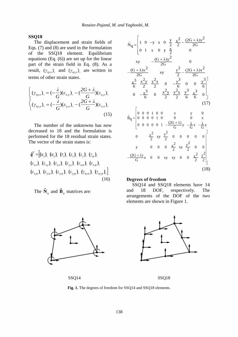
Degrees of freedom
SSQ14 and SSQ18 elements have 14
and 18 DOF, respectively. The
arrangements of the DOF of the two
elements are shown in Figure 1.
SSQ14 SSQ18
Fig. 1. The degrees of freedom for SSQ14 and SSQ18 elements.

Civil Engineering Infrastructures Journal, 48(1): 133-156, June 2015
139
Finding the stiffness matrix
By allotting qN , qB , and q matrices for
each SSQ14 and SSQ18 element, their
stiffness matrices can be found. The
displacement unknowns are denoted by the
vector of the strain states ( q ). The nodal
DOF are denoted by vector D. The
relationship q.NU q holds between the
displacement functions in the x and y
directions, U, and the displacement
unknowns ( q ). The nodal rotations are
defined as )(y
y
u
x
u
2
1 x
. The nodal
displacements are the shifts in the x and y
directions plus the nodal rotation. The
following equations connect the nodal
DOF and the displacement unknowns:
q.GD q (19)
D.Gq1
q
(20)
The qG matrix is obtained by inserting
the nodal coordinates of each element into
the corresponding qN and sets up the
relation between the vector of the strain
states and the nodal displacement vector.
Consequently, the displacement boundary
conditions can be entered into the
formulation. The displacement and strain
fields for the nodal displacement vector in
matrix form are:
D.N)D.G.(Nq.NU 1
qqq (21)
D.B)D.G( .Bq.Bε 1
qqq (22)
where 1
G.NN and
1
G.BB .
The functional of the potential energy for
the elasticity matrix of E is:
dv dv2
1
dvdv2
1
TTT
T
TT
F.NDD)B.E.B(D
F.Uε.E.εΠ
(23)
Optimization of the potential energy
results in:
0D
(24)
0F.ND)B.E.B(D
dv dv T
T (25)
This equation can be expressed as:
dv dv TT
F.ND)B.E.B( (26)
Stiffness matrix K and nodal load
vector P are:
dvT
B.E.BK (27)
dvTF.NP (28)
The shape function matrices are defined
by N. Analytical schemes are used to find
the stiffness matrix. Using triangular
coordinates, the quadrilateral element is
divided into two triangular shapes and the
stiffness matrix is easily integrated.
NUMERICAL TESTS
The abilities of the proposed elements
were evaluated using 12 difficult test
problems. To demonstrate the power of
new formulation, the answers of the good
elements of other researchers were used
for comparison. These elements are:
4-node isoparametric element: Q4
(Chen et al., 2004; Wisniewski and Turska,
2009)
Element with internal parameters
formulated by QACM-I: AGQ6-II (Cen et
al., 2009; Chen et al., 2004)
Element with internal parameters
formulated by QACM-I: QACM4 (Cen et
al., 2007)
Quadrilateral element in
MSC/NASTRAN: CQUAD4 (Choi et al.,
2006; MacNeal, 1971)
4-node isoparametric element with
internal parameters: HL (Bergan and
Felippa, 1985; Cook, 1974)

Rezaiee-Pajand, M. and Yaghoobi, M.
140
Stress hybrid element: PS (Cen et al.,
2009; Chen et al., 2004; Pian and
Sumihara, 1984)
Triangular element with rotational
DOF: FF(α=1.5, β=0.5) (Bergan and Felippa,
1985)
Allman’s element: ALLMAN (Allman,
1984; Choo et al., 2006; Cook, 1986)
Membrane element with drilling DOF:
Q4S (Cen et al., 2009; MacNeal and
Harder, 1988)
Hybrid element with internal
parameters: NQ6 (Cen et al., 2009; Wu et
al., 1987)
Non-conforming isoparametric element
with internal parameters: QM6 (Cen et al.,
2009; Chen et al., 2004; Choi et al., 2006;
Taylor et al., 1976)
Non-conforming isoparametric element
with internal parameters: Q6 (Cen et al.,
2007, 2009; Wilson et al., 1973)
Ibrahimbegovic plane element with true
rotation: IB (Choi et al., 2006;
Ibrahimgovic et al., 1990)
Membrane element with drilling DOF:
D-type (Cen et al., 2009; Ibrahimgovic et
al., 1990)
Hybrid Trefftz plane element: HT
(Choo et al., 2006; Jirousek and
Venkatesh, 1992)
Assumed strain element: PEAS7
(Andelfinger and Ramm, 1993; Chen et al.,
2004)
Modified enhanced assumed strain
element: MEAS (Choi et al., 2006; Choo et
al., 2006; Yeo and Lee, 1997)
Quadrilateral element with two
enhanced strain modes: QE-2 (Cen et al.,
2009; Piltner and Taylor, 1995, 1997 )
Assumed strain element: B-Q4E (Cen et
al., 2009; Piltner and Taylor, 1997)
Quadrilateral hybrid Trefftz element
with rotational DOF: HTD (Choo et al.,
2006)
HR element with 5 modes in skew
coordinates: HR5-S (Wisniewski and
Turska, 2006, 2009)
Enhanced assumed displacement
gradient element with 4 modes: EADG4
(Wisniewski and Turska, 2008, 2009)
Mixed 4-node elements based on Hu-
Washizu functional: HW12-S, HW14-S,
HW10-N, HW14-N, HW18 (Wisniewski
and Turska, 2009)
Free formulation quadrilateral: FFQ
(Felippa, 2003; Nygard, 1986)
4-node membrane elements with
analytical element stiffness matrix: QAC-
ATF4 (Cen et al., 2009)
8-node membrane element based on 3
quadrilateral area coordinate methods
QACM-I, -II, and -III: CQAC-Q8 (Long et
al., 2010)
8-node element formulated using
quadrilateral area coordinates: QACM8
(Cen et al., 2007)
Conventional 8-node quadrilateral
isoparametric elements: Q8
Hybrid stress element using first Piola–
Kirchhoff stresses of degree 4 and
displacements of degree 2: Hybrid stress
element with dp=4, dv=2 (Santos and
Moitinho de Almeida, 2014)
Cantilever Beam with Distortion
Parameter
The cantilever beam shown in Figure 2
has two elements, the shapes of which vary
with the variation of distorted parameter e.
The existence of coarse mesh, an aspect
ratio of 2.5 for e = 0 and intense distortions
in the mesh make it an appropriate test for
evaluating the sensitivity of the distortion
of the mesh. The modulus of elasticity is
75, Poisson’s ratio is 0.25, and thickness of
the structure is 1.
Figure 3 shows analysis of the
cantilever beam under 3 loadings at the
free end of the beam. This structure has an
axial force of 1 at the free end of the beam
for the constant stress patch test. For the
bending patch test with linear stress, a
moment equal to 1 is applied to the free
end of the beam. A shear load equal to 1 is
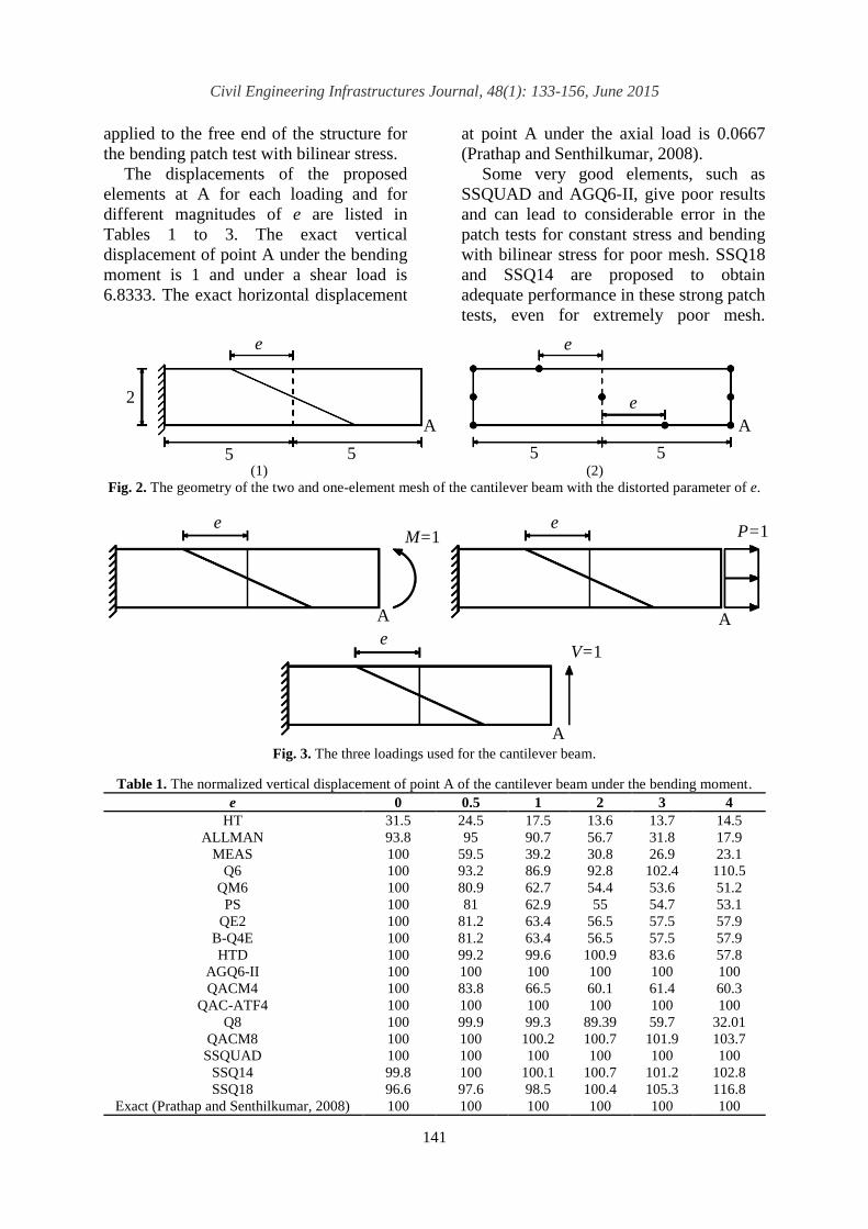
Civil Engineering Infrastructures Journal, 48(1): 133-156, June 2015
141
applied to the free end of the structure for
the bending patch test with bilinear stress.
The displacements of the proposed
elements at A for each loading and for
different magnitudes of e are listed in
Tables 1 to 3. The exact vertical
displacement of point A under the bending
moment is 1 and under a shear load is
6.8333. The exact horizontal displacement
at point A under the axial load is 0.0667
(Prathap and Senthilkumar, 2008).
Some very good elements, such as
SSQUAD and AGQ6-II, give poor results
and can lead to considerable error in the
patch tests for constant stress and bending
with bilinear stress for poor mesh. SSQ18
and SSQ14 are proposed to obtain
adequate performance in these strong patch
tests, even for extremely poor mesh.
(1) (2)
Fig. 2. The geometry of the two and one-element mesh of the cantilever beam with the distorted parameter of e.
Fig. 3. The three loadings used for the cantilever beam.
Table 1. The normalized vertical displacement of point A of the cantilever beam under the bending moment.
4 3 2 1 0.5 0 e
14.5 13.7 13.6 17.5 24.5 31.5 HT
17.9 31.8 56.7 90.7 95 93.8 ALLMAN
23.1 26.9 30.8 39.2 59.5 100 MEAS
110.5 102.4 92.8 86.9 93.2 100 Q6
51.2 53.6 54.4 62.7 80.9 100 QM6
53.1 54.7 55 62.9 81 100 PS
57.9 57.5 56.5 63.4 81.2 100 QE2
57.9 57.5 56.5 63.4 81.2 100 B-Q4E
57.8 83.6 100.9 99.6 99.2 100 HTD
100 100 100 100 100 100 AGQ6-II
60.3 61.4 60.1 66.5 83.8 100 QACM4
100 100 100 100 100 100 QAC-ATF4
32.01 59.7 89.39 99.3 99.9 100 Q8
103.7 101.9 100.7 100.2 100 100 QACM8
100 100 100 100 100 100 SSQUAD
102.8 101.2 100.7 100.1 100 99.8 SSQ14
116.8 105.3 100.4 98.5 97.6 96.6 SSQ18
100 100 100 100 100 100 Exact (Prathap and Senthilkumar, 2008)
e
2
5 5
e
e
5 5
A A
M=1 P=1
V=1
e e
e
A A
A
Rezaiee-Pajand, M. and Yaghoobi, M.
142
Table 2. The normalized horizontal displacement of point A of the cantilever beam under the axial load.
4 3 2 1 0 e
2.084 1.544 1.225 1.054 1.000 AGQ6-II
2.082 1.540 1.218 1.046 0.991 SSQUAD
1.581 1.295 1.123 1.065 1.064 SSQ14
1.014 1.014 1.014 1.010 1.002 SSQ18
1.000 1.000 1.000 1.000 1.000 Exact (Prathap and Senthilkumar, 2008)
Table 3. The normalized vertical displacement of point A of the cantilever beam under the shear load on the free end.
4 3 2 1 0 e
1.5916 1.2370 1.0520 0.9650 0.9396 AGQ6-II
0.3255 0.5478 0.7992 0.9298 0.9765 Q8
0.8421 0.8489 0.8830 0.9483 0.9765 QACM8
1.5899 1.2344 1.0493 0.9635 0.9390 SSQUAD
1.0415 1.0080 0.9948 0.9885 0.9849 SSQ14
1.1136 1.0284 0.9915 0.9740 0.9458 SSQ18
1.0000 1.0000 1.0000 1.0000 1.0000 Exact (Prathap and Senthilkumar, 2008)
SSQ18 showed less than 5% error in
analysis of the cantilever beam under a
moment for magnitudes of e equal to 0,
0.5, 1, 2 and 3. The errors for the beam
under axial and shear loading at
magnitudes of e equal to 4 were 1% and
11%, respectively. The errors by AGQ6-II
were 108% and 59%. These outcomes
demonstrate that SSQ14 results for shear
and moment loading showed better
accuracy than the SSQ18 results.
A cantilever beam was analyzed using
SSQ18 in one-element mesh (Figure 2b).
The displacement at point A by SSQ18 for
V, P and M loadings and different
magnitudes of e are listed in Table 4.
These results show the insensitivity of
SSQ18 to the arrangement of nodes.
MacNeal Thin Beam
This test evaluates the decrease in
accuracy for parallelogram-shaped and
trapezoidal mesh. Figure 4 shows a thin
cantilever beam with rectangular,
parallelogram-shaped and trapezoidal
mesh. MacNeal suggested this benchmark
for testing sensitivity to distortion in the
mesh for quadrilateral elements (MacNeal
and Harder, 1985). Six elements are used
for analysis. The aspect ratio of the
elements in the rectangular mesh is 5.
Since a high aspect ratio creates distortion
in the parallelogram-shaped and
trapezoidal mesh, it is an appropriate test
to evaluate the efficiency of the elements.
The modulus of elasticity is 10000000,
Poisson’s ratio is 0.3 and thickness of the
structure is 0.1. This problem has two
types of loading; pure bending under a
bending moment and bending under a
shear force of one at the free end of the
beam. The exact vertical displacement at
point A of the free end of the beam for
moment and shear loading are 0.0054 and
0.1081, respectively (Cen et al., 2009).
Table 4. The normalized displacement of point A of the cantilever beam in the one-element SSQ18 mesh (Exact
solution (Prathap and Senthilkumar, 2008) is equal to 1.0000).
e Load
4 3 2 1 0
0.9442 0.9442 0.9442 0.9442 0.9442 V
0.9944 0.9944 0.9944 0.9944 0.9944 P
0.9612 0.9612 0.9612 0.9612 0.9612 M
Civil Engineering Infrastructures Journal, 48(1): 133-156, June 2015
143
Fig. 4. The rectangular, parallelogram-shaped and trapezoidal meshes of the MacNeal beam.
Table 5 shows that for both types of
loading, SSQ14 and SSQ18 in trapezoidal
and parallelogram-shaped mesh showed no
sensitivity to distortion. The results of
other elements showed high sensitivity to
distortion such that the error of the results
for trapezoidal mesh increased
significantly for both types of loading.
SSQ18 provided an accurate response for
both types of loading and for all types of
mesh. Furthermore, SSQ14 showed a low
error for both types of loading.
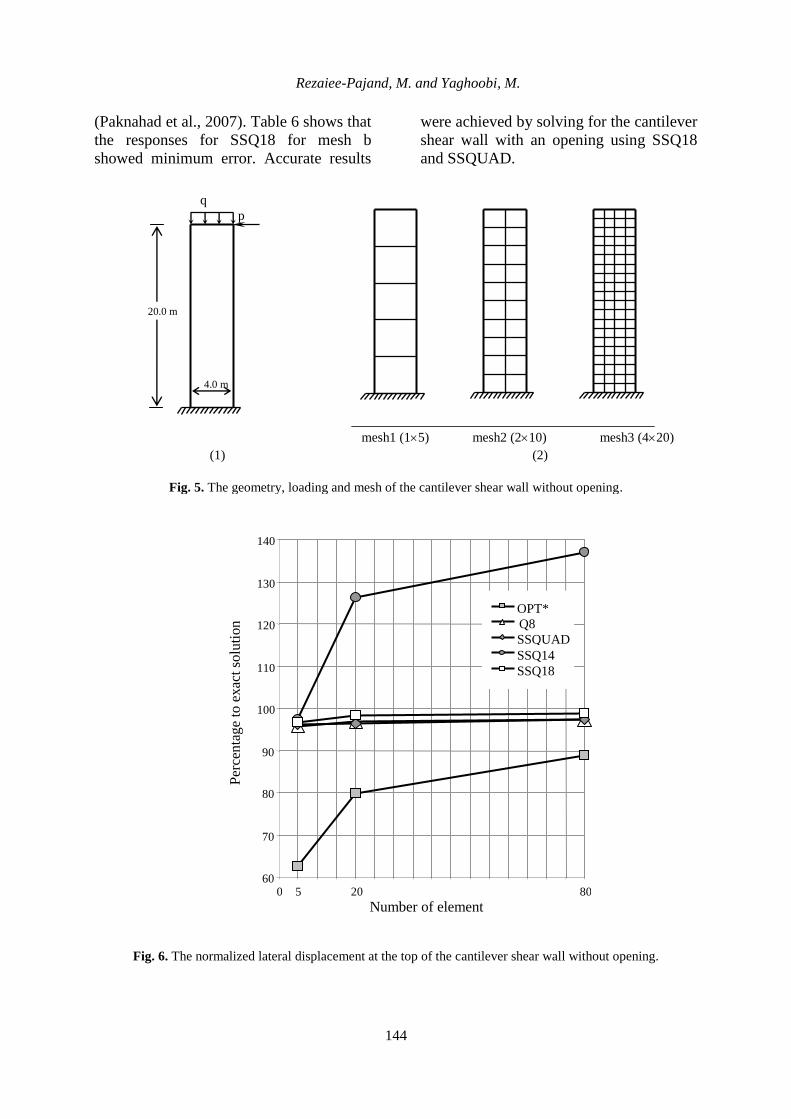
Shear Wall without Opening
SSQ14 and SSQ18 are used to analyze
a cantilever shear wall without an opening.
The geometry and loading of this wall is
shown in Figure 5a. The elasticity modulus
is 20,000,000 kN/m2 and the structural
Poisson’s ratio is 0.2. Loads P and q are
100 kN and 500 kN, respectively.
The shear wall is analyzed for the types
of mesh shown in Figure 5b. The lateral
displacement at the top of the shear wall is
calculated for the types of mesh using
SSQUAD, SSQ14, SSQ18 and Q8
elements. For comparison, the opt* element
was also used and its results are available
elsewhere (Paknahad et al., 2007). The
powerful opt* element was specifically
created for analysis of shear walls.
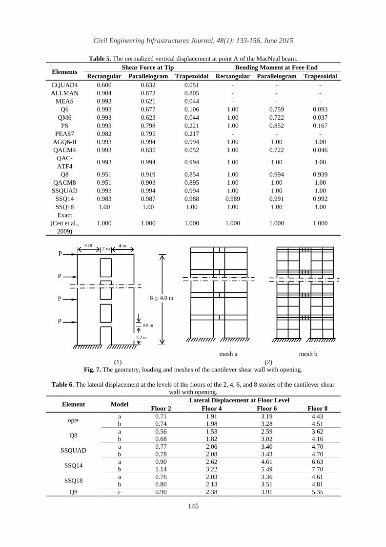
Figure 6 shows the high accuracy of the
SSQ18 element. For refined mesh, SSQ14
produced larger responses. This indicates
that the rotational DOF and satisfying the
equilibrium condition in the domain of the
second-order field decreased the ability of
SSQ14. To eliminate this weakness, the
equilibrium condition was satisfied in the
linear displacement field.
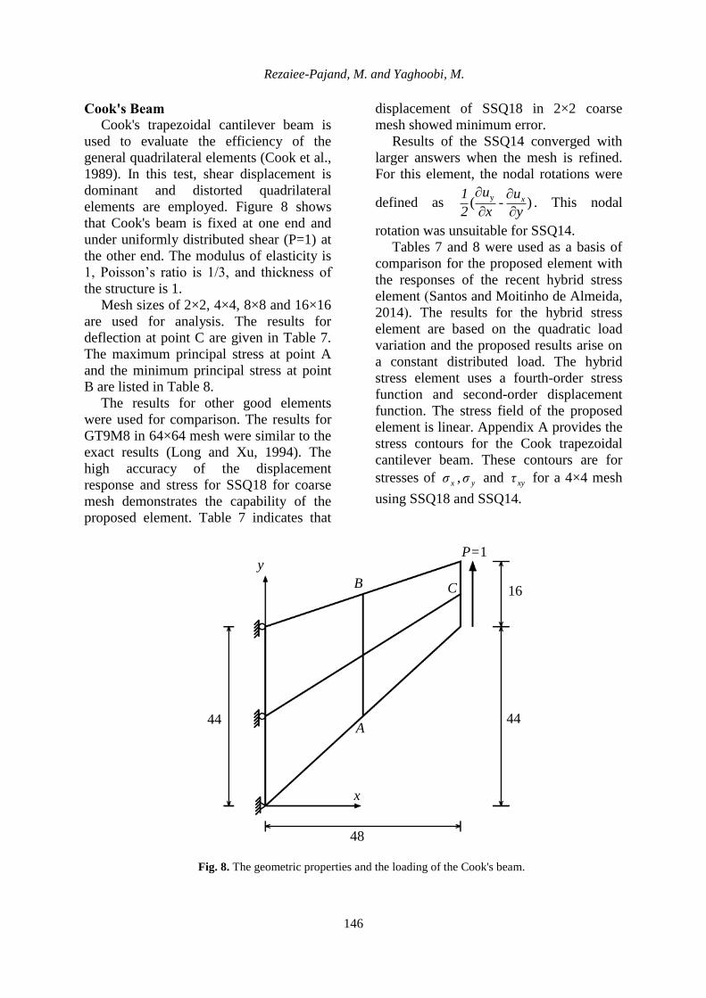
Shear Wall with Opening The geometry and loading of a
cantilever shear wall with an opening is
shown in Figure 7a. The modulus of
elasticity is 20,000,000 kN/m2 and the
Poisson’s ratio is 0.25. The thickness of
the wall is 0.4 m and force P is 500 kN.
Two types of mesh, a and b, are used in the
analysis of this shear wall (Figure 7b).
SSQ14 and SSQ18 were used to calculate
the lateral displacement at floor level on
stories 2, 4, 6, and 8 for both types of
mesh. The opt* element results were again
used as a means of comparison (Paknahad
et al., 2007).
The results for SSQUAD and Q8 are
shown in Table 6. For assessment
purposes, the results for Q8 were
calculated for fine mesh for this shear wall.
The shear wall was divided into 10×10
rectangular elements and the mesh denoted
as c and had 26880 Q8 elements
1
1
1
1
1
1
1
1
1
45
45
6
0.2 A
Rezaiee-Pajand, M. and Yaghoobi, M.
144
(Paknahad et al., 2007). Table 6 shows that
the responses for SSQ18 for mesh b
showed minimum error. Accurate results
were achieved by solving for the cantilever
shear wall with an opening using SSQ18
and SSQUAD.
mesh1 (15) mesh2 (210) mesh3 (420)
(1) (2)
Fig. 5. The geometry, loading and mesh of the cantilever shear wall without opening.
Fig. 6. The normalized lateral displacement at the top of the cantilever shear wall without opening.
q
p
20.0 m
4.0 m
60
70
80
90
100
110
120
130
140
0 5 20 80
Per
centa
ge
to e
xac
t so
luti
on
OPT*
Q8
SSQUAD
SSQ14
SSQ18
Number of element
Civil Engineering Infrastructures Journal, 48(1): 133-156, June 2015
145
Table 5. The normalized vertical displacement at point A of the MacNeal beam.
Bending Moment at Free End Shear Force at Tip Elements
Trapezoidal Parallelogram Rectangular Trapezoidal Parallelogram Rectangular
- - - 0.051 0.632 0.600 CQUAD4
- - - 0.805 0.873 0.904 ALLMAN
- - - 0.044 0.621 0.993 MEAS
0.093 0.759 1.00 0.106 0.677 0.993 Q6
0.037 0.722 1.00 0.044 0.623 0.993 QM6
0.167 0.852 1.00 0.221 0.798 0.993 PS
- - - 0.217 0.795 0.982 PEAS7
1.00 1.00 1.00 0.994 0.994 0.993 AGQ6-II
0.046 0.722 1.00 0.052 0.635 0.993 QACM4
1.00 1.00 1.00 0.994 0.994 0.993 QAC-
ATF4
0.939 0.994 1.00 0.854 0.919 0.951 Q8
1.00 1.00 1.00 0.895 0.903 0.951 QACM8
1.00 1.00 1.00 0.994 0.994 0.993 SSQUAD
0.992 0.991 0.989 0.988 0.987 0.983 SSQ14
1.00 1.00 1.00 1.00 1.00 1.00 SSQ18
1.000 1.000 1.000 1.000 1.000 1.000
Exact
(Cen et al.,
2009)
mesh a mesh b
(1) (2) Fig. 7. The geometry, loading and meshes of the cantilever shear wall with opening.
Table 6. The lateral displacement at the levels of the floors of the 2, 4, 6, and 8 stories of the cantilever shear
wall with opening.
Lateral Displacement at Floor Level Model Element
Floor 8 Floor 6 Floor 4 Floor 2
4.43
4.51
3.19
3.28
1.91
1.98
0.71
0.74
a
b opt
3.62
4.16
2.59
3.02
1.53
1.82
0.56
0.68
a
b Q8
4.70
4.70
3.40
3.43
2.06
2.08
0.77
0.78
a
b SSQUAD
6.63
7.70
4.61
5.49
2.62
3.22
0.90
1.14
a
b SSQ14
4.61
4.81
3.36
3.51
2.03
2.13
0.76
0.80
a
b SSQ18
5.35 3.91 2.38 0.90 c Q8
4 m 4 m 2 m
8 @ 4.0 m
P
P
P
P 0.8 m
3.2 m
Rezaiee-Pajand, M. and Yaghoobi, M.
146
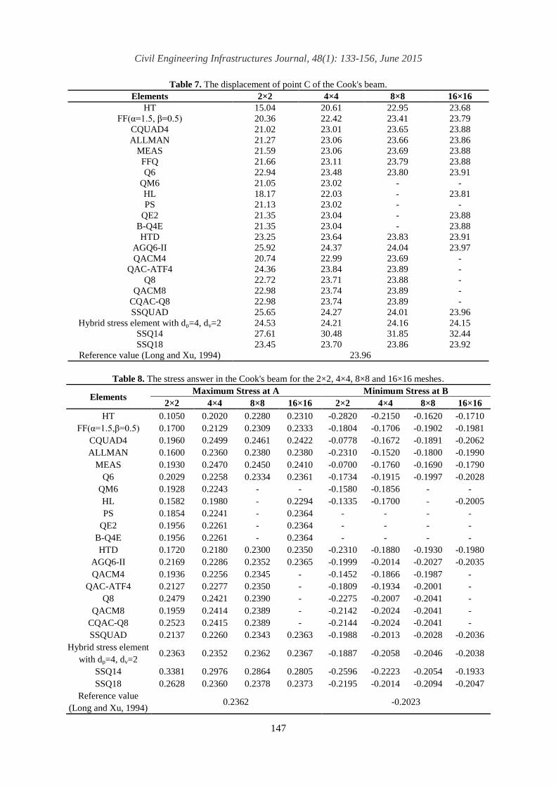
Cook's Beam
Cook's trapezoidal cantilever beam is
used to evaluate the efficiency of the
general quadrilateral elements (Cook et al.,
1989). In this test, shear displacement is
dominant and distorted quadrilateral
elements are employed. Figure 8 shows
that Cook's beam is fixed at one end and
under uniformly distributed shear (P=1) at
the other end. The modulus of elasticity is
1, Poisson’s ratio is 1/3, and thickness of
the structure is 1.
Mesh sizes of 2×2, 4×4, 8×8 and 16×16
are used for analysis. The results for
deflection at point C are given in Table 7.
The maximum principal stress at point A
and the minimum principal stress at point
B are listed in Table 8.
The results for other good elements
were used for comparison. The results for
GT9M8 in 64×64 mesh were similar to the
exact results (Long and Xu, 1994). The
high accuracy of the displacement
response and stress for SSQ18 for coarse
mesh demonstrates the capability of the
proposed element. Table 7 indicates that
displacement of SSQ18 in 2×2 coarse
mesh showed minimum error.
Results of the SSQ14 converged with
larger answers when the mesh is refined.
For this element, the nodal rotations were
defined as )(y
y
u-
x
u
2
1 x
. This nodal
rotation was unsuitable for SSQ14.
Tables 7 and 8 were used as a basis of
comparison for the proposed element with
the responses of the recent hybrid stress
element )Santos and Moitinho de Almeida,
2014(. The results for the hybrid stress
element are based on the quadratic load
variation and the proposed results arise on
a constant distributed load. The hybrid
stress element uses a fourth-order stress
function and second-order displacement
function. The stress field of the proposed
element is linear. Appendix A provides the
stress contours for the Cook trapezoidal
cantilever beam. These contours are for
stresses of xσ , yσ and xyτ for a 4×4 mesh
using SSQ18 and SSQ14.
Fig. 8. The geometric properties and the loading of the Cook's beam.
44
48
44
16
P=1
x
y
A
B C
Civil Engineering Infrastructures Journal, 48(1): 133-156, June 2015
147
Table 7. The displacement of point C of the Cook's beam.
16×16 8×8 4×4 2×2 Elements
23.68 22.95 20.61 15.04 HT
23.79 23.41 22.42 20.36 FF(α=1.5, β=0.5)
23.88 23.65 23.01 21.02 CQUAD4
23.86 23.66 23.06 21.27 ALLMAN
23.88 23.69 23.06 21.59 MEAS
23.88 23.79 23.11 21.66 FFQ
23.91 23.80 23.48 22.94 Q6
- - 23.02 21.05 QM6
23.81 - 22.03 18.17 HL
- - 23.02 21.13 PS
23.88 - 23.04 21.35 QE2
23.88 - 23.04 21.35 B-Q4E
23.91 23.83 23.64 23.25 HTD
23.97 24.04 24.37 25.92 AGQ6-II
- 23.69 22.99 20.74 QACM4
- 23.89 23.84 24.36 QAC-ATF4
- 23.88 23.71 22.72 Q8
- 23.89 23.74 22.98 QACM8
- 23.89 23.74 22.98 CQAC-Q8
23.96 24.01 24.27 25.65 SSQUAD
24.15 24.16 24.21 24.53 Hybrid stress element with dp=4, dv=2
32.44 31.85 30.48 27.61 SSQ14
23.92 23.86 23.70 23.45 SSQ18
23.96 Reference value (Long and Xu, 1994)
Table 8. The stress answer in the Cook's beam for the 2×2, 4×4, 8×8 and 16×16 meshes.
Minimum Stress at B Maximum Stress at A Elements
16×16 8×8 4×4 2×2 16×16 8×8 4×4 2×2
-0.1710 -0.1620 -0.2150 -0.2820 0.2310 0.2280 0.2020 0.1050 HT
-0.1981 -0.1902 -0.1706 -0.1804 0.2333 0.2309 0.2129 0.1700 FF(α=1.5,β=0.5)
-0.2062 -0.1891 -0.1672 -0.0778 0.2422 0.2461 0.2499 0.1960 CQUAD4
-0.1990 -0.1800 -0.1520 -0.2310 0.2380 0.2380 0.2360 0.1600 ALLMAN
-0.1790 -0.1690 -0.1760 -0.0700 0.2410 0.2450 0.2470 0.1930 MEAS
-0.2028 -0.1997 -0.1915 -0.1734 0.2361 0.2334 0.2258 0.2029 Q6
- - -0.1856 -0.1580 - - 0.2243 0.1928 QM6
-0.2005 - -0.1700 -0.1335 0.2294 - 0.1980 0.1582 HL
- - - - 0.2364 - 0.2241 0.1854 PS
- - - - 0.2364 - 0.2261 0.1956 QE2
- - - - 0.2364 - 0.2261 0.1956 B-Q4E
-0.1980 -0.1930 -0.1880 -0.2310 0.2350 0.2300 0.2180 0.1720 HTD
-0.2035 -0.2027 -0.2014 -0.1999 0.2365 0.2352 0.2286 0.2169 AGQ6-II
- -0.1987 -0.1866 -0.1452 - 0.2345 0.2256 0.1936 QACM4
- -0.2001 -0.1934 -0.1809 - 0.2350 0.2277 0.2127 QAC-ATF4
- -0.2041 -0.2007 -0.2275 - 0.2390 0.2421 0.2479 Q8
- -0.2041 -0.2024 -0.2142 - 0.2389 0.2414 0.1959 QACM8
- -0.2041 -0.2024 -0.2144 - 0.2389 0.2415 0.2523 CQAC-Q8
-0.2036 -0.2028 -0.2013 -0.1988 0.2363 0.2343 0.2260 0.2137 SSQUAD
-0.2038 -0.2046 -0.2058 -0.1887 0.2367 0.2362 0.2352 0.2363 Hybrid stress element
with dp=4, dv=2
-0.1933 -0.2054 -0.2223 -0.2596 0.2805 0.2864 0.2976 0.3381 SSQ14
-0.2047 -0.2094 -0.2014 -0.2195 0.2373 0.2378 0.2360 0.2628 SSQ18
-0.2023 0.2362 Reference value
(Long and Xu, 1994)
Rezaiee-Pajand, M. and Yaghoobi, M.
148
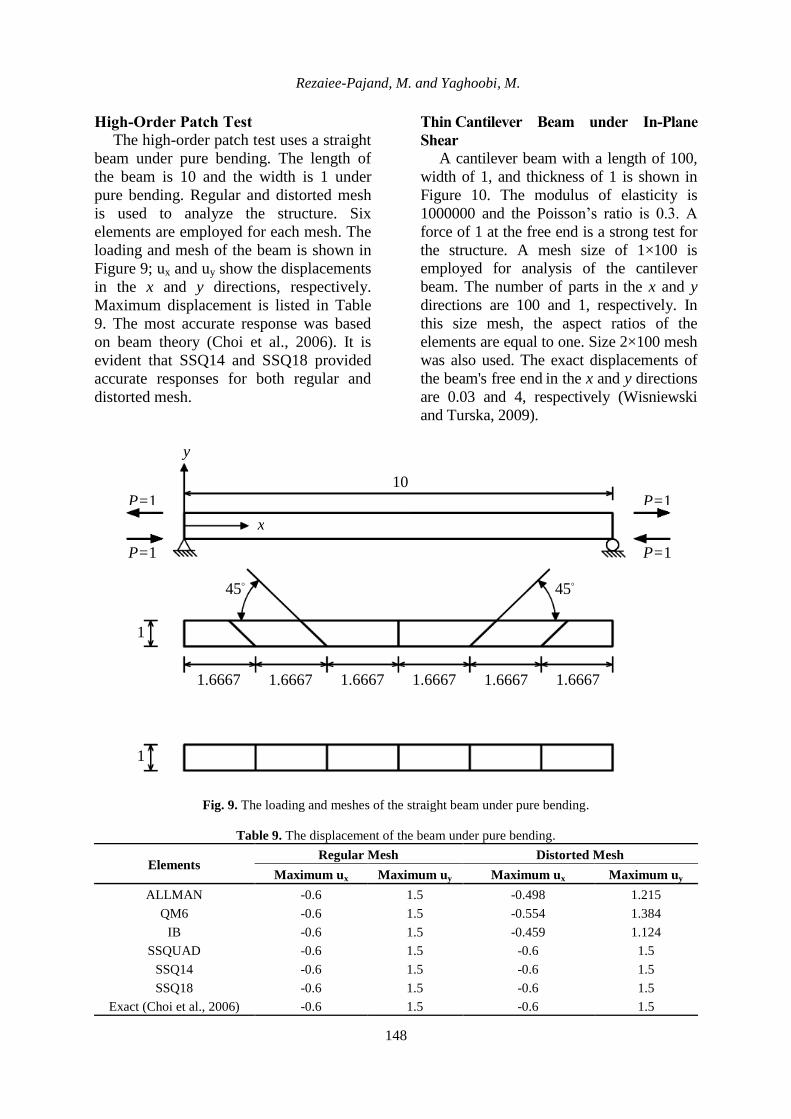
High-Order Patch Test
The high-order patch test uses a straight
beam under pure bending. The length of
the beam is 10 and the width is 1 under
pure bending. Regular and distorted mesh
is used to analyze the structure. Six
elements are employed for each mesh. The
loading and mesh of the beam is shown in
Figure 9; ux and uy show the displacements
in the x and y directions, respectively.
Maximum displacement is listed in Table
9. The most accurate response was based
on beam theory (Choi et al., 2006). It is
evident that SSQ14 and SSQ18 provided
accurate responses for both regular and
distorted mesh.
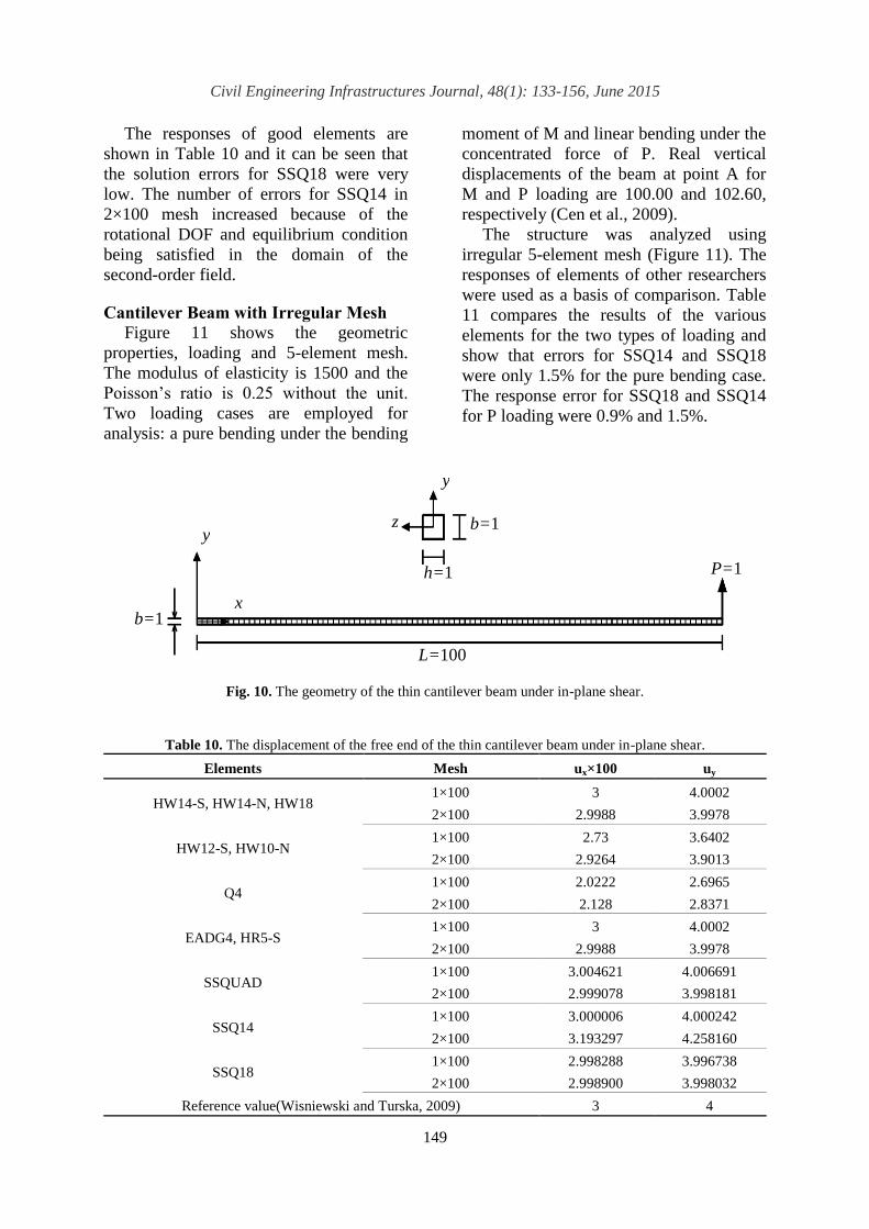
Thin Cantilever Beam under In-Plane
Shear
A cantilever beam with a length of 100,
width of 1, and thickness of 1 is shown in
Figure 10. The modulus of elasticity is
1000000 and the Poisson’s ratio is 0.3. A
force of 1 at the free end is a strong test for
the structure. A mesh size of 1×100 is
employed for analysis of the cantilever
beam. The number of parts in the x and y
directions are 100 and 1, respectively. In
this size mesh, the aspect ratios of the
elements are equal to one. Size 2×100 mesh
was also used. The exact displacements of
the beam's free end in the x and y directions
are 0.03 and 4, respectively (Wisniewski
and Turska, 2009).
Fig. 9. The loading and meshes of the straight beam under pure bending.
Table 9. The displacement of the beam under pure bending.
Distorted Mesh Regular Mesh Elements
Maximum uy Maximum ux Maximum uy Maximum ux
1.215 -0.498 1.5 -0.6 ALLMAN
1.384 -0.554 1.5 -0.6 QM6
1.124 -0.459 1.5 -0.6 IB
1.5 -0.6 1.5 -0.6 SSQUAD
1.5 -0.6 1.5 -0.6 SSQ14
1.5 -0.6 1.5 -0.6 SSQ18
1.5 -0.6 1.5 -0.6 Exact (Choi et al., 2006)
1.6667 1.6667 1.6667 1.6667 1.6667 1.6667
45 45
1
1
10
P=1
P=1
P=1
P=1
x
y
Civil Engineering Infrastructures Journal, 48(1): 133-156, June 2015
149
The responses of good elements are
shown in Table 10 and it can be seen that
the solution errors for SSQ18 were very
low. The number of errors for SSQ14 in
2×100 mesh increased because of the
rotational DOF and equilibrium condition
being satisfied in the domain of the
second-order field.
Cantilever Beam with Irregular Mesh
Figure 11 shows the geometric
properties, loading and 5-element mesh.
The modulus of elasticity is 1500 and the
Poisson’s ratio is 0.25 without the unit.
Two loading cases are employed for
analysis: a pure bending under the bending
moment of M and linear bending under the
concentrated force of P. Real vertical
displacements of the beam at point A for
M and P loading are 100.00 and 102.60,
respectively (Cen et al., 2009).
The structure was analyzed using
irregular 5-element mesh (Figure 11). The
responses of elements of other researchers
were used as a basis of comparison. Table
11 compares the results of the various
elements for the two types of loading and
show that errors for SSQ14 and SSQ18
were only 1.5% for the pure bending case.
The response error for SSQ18 and SSQ14
for P loading were 0.9% and 1.5%.
Fig. 10. The geometry of the thin cantilever beam under in-plane shear.
Table 10. The displacement of the free end of the thin cantilever beam under in-plane shear.
uy ux×100 Mesh Elements
4.0002 3 1×100 HW14-S, HW14-N, HW18
3.9978 2.9988 2×100
3.6402 2.73 1×100 HW12-S, HW10-N
3.9013 2.9264 2×100
2.6965 2.0222 1×100 Q4
2.8371 2.128 2×100
4.0002 3 1×100 EADG4, HR5-S
3.9978 2.9988 2×100
4.006691 3.004621 1×100 SSQUAD
3.998181 2.999078 2×100
4.000242 3.000006 1×100 SSQ14
4.258160 3.193297 2×100
3.996738 2.998288 1×100 SSQ18
3.998032 2.998900 2×100
4 3 Reference value(Wisniewski and Turska, 2009)
b=1
L=100
b=1
h=1
y
x
y
z
P=1

Rezaiee-Pajand, M. and Yaghoobi, M.
150
Fig. 11. The cantilever beam with irregular mesh.
Table 11. The displacement of the cantilever beam in two loading cases.
P M Elements
100.40 98.40 Q6
97.98 96.07 QM6
98.00 96.10 NQ6
98.05 96.18 PS
98.26 96.50 QE-2
98.26 96.5 B-Q4E
102.7 100.0 AGQ6-II
98.0 96.0 QACM4
102.4 100.0 QAC-ATF4
101.5 99.7 Q8
102.8 101.3 QACM8
102.79 100.00 SSQUAD
104.16 101.66 SSQ14
103.52 101.48 SSQ18
102.60 100.00 Exact(Cen et al., 2009)
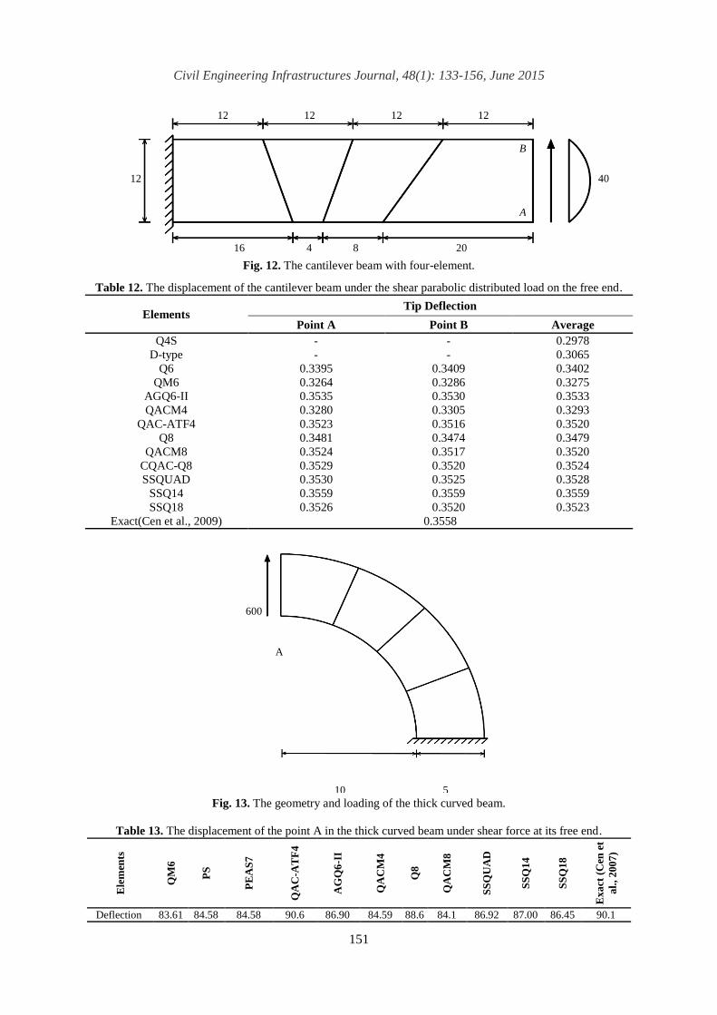
Cantilever beam with four-element In the mesh of the cantilever beam of
this test, 4 irregular Cantilever beam with 4 elements quadrilateral elements are used. The geometry of the beam is shown in Figure 12. The modulus of elasticity is 30000, the Poisso’s ratio is 0.25, and the thickness of the beam is 1. The free end of the beam is under a parabolic distributed shear load. The vertical displacement at points A and B are listed in Table 12. The displacement of the beam at both A and B points is equal to 0.3558 (Cen et al., 2009). This test evaluates the capability of the elements for shear deformations for an irregular mesh. The low error of the SSQ14 and SSQ18 elements is evident in
Table 12. These errors for SSQ18 and SSQ14 elements were 1% and 0.03%.
Thick Curved Beam
A thick curved beam is analyzed in
Figure 13 under a shear force of 600 on the
free end. The modulus of elasticity is 1000,
Poisson’s ratio is 0, and the thickness of
the structure 1. A 4-element mesh is used
for analysis. The vertical displacement at
point A is listed in Table 13. The accurate
response for vertical displacement at point
A is 90.1 (Cen et al., 2007). The response
error for SSQ14 and SSQ18 was 3.5% and
4%, respectively.
P=150 P=150
P=150
2 2 1 1 4
1 1 2 3 3
2
M=2000
Civil Engineering Infrastructures Journal, 48(1): 133-156, June 2015
151
Fig. 12. The cantilever beam with four-element.
Table 12. The displacement of the cantilever beam under the shear parabolic distributed load on the free end.
Tip Deflection Elements
Average Point B Point A
0.2978 - - Q4S
0.3065 - - D-type
0.3402 0.3409 0.3395 Q6
0.3275 0.3286 0.3264 QM6
0.3533 0.3530 0.3535 AGQ6-II
0.3293 0.3305 0.3280 QACM4
0.3520 0.3516 0.3523 QAC-ATF4
0.3479 0.3474 0.3481 Q8
0.3520 0.3517 0.3524 QACM8
0.3524 0.3520 0.3529 CQAC-Q8
0.3528 0.3525 0.3530 SSQUAD
0.3559 0.3559 0.3559 SSQ14
0.3523 0.3520 0.3526 SSQ18
0.3558 Exact(Cen et al., 2009)
Fig. 13. The geometry and loading of the thick curved beam.
Table 13. The displacement of the point A in the thick curved beam under shear force at its free end.
Ex
act
(C
en e
t
al.
, 2
00
7)
SS
Q1
8
SS
Q1
4
SS
QU
AD
QA
CM
8
Q8
QA
CM
4
AG
Q6
-II
QA
C-A
TF
4
PE
AS
7
PS
QM
6
Ele
men
ts
90.1 86.45 87.00 86.92 84.1 88.6 84.59 86.90 90.6 84.58 84.58 83.61 Deflection
600
10 5
A
12 12 12 12
16 4 8 20
12 40
A
B
Rezaiee-Pajand, M. and Yaghoobi, M.
152
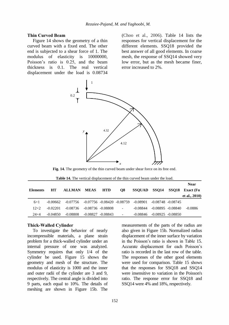
Thin Curved Beam
Figure 14 shows the geometry of a thin
curved beam with a fixed end. The other
end is subjected to a shear force of 1. The
modulus of elasticity is 10000000,
Poisson’s ratio is 0.25, and the beam
thickness is 0.1. The real vertical
displacement under the load is 0.08734
(Choo et al., 2006). Table 14 lists the
responses for vertical displacement for the
different elements. SSQ18 provided the
best answer of all good elements. In coarse
mesh, the response of SSQ14 showed very
low error, but as the mesh became finer,
error increased to 2%.
Fig. 14. The geometry of the thin curved beam under shear force on its free end.
Table 14. The vertical displacement of the thin curved beam under the load.
Near
Exact (Fu
et al., 2010)
SSQ18 SSQ14 SSQUAD Q8 HTD MEAS ALLMAN HT Elements
-0.0886
-0.08745 -0.08748 -0.08901 -0.08759 -0.08420 -0.07756 -0.07756 -0.00662 6×1
-0.08840 -0.08895 -0.08844 - -0.08808 -0.08736 -0.08736 -0.02201 12×2
-0.08850 -0.08925 -0.08846 - -0.08843 -0.08827 -0.08808 -0.04850 24×4
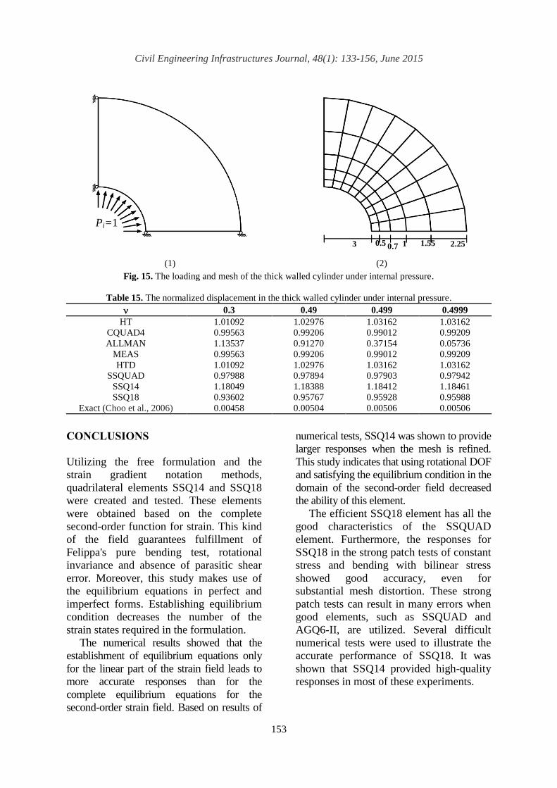
Thick-Walled Cylinder
To investigate the behavior of nearly
incompressible materials, a plane strain
problem for a thick-walled cylinder under an
internal pressure of one was analyzed.
Symmetry requires that only 1/4 of the
cylinder be used. Figure 15 shows the
geometry and mesh of the structure. The
modulus of elasticity is 1000 and the inner
and outer radii of the cylinder are 3 and 9,
respectively. The central angle is divided into
9 parts, each equal to 10%. The details of
meshing are shown in Figure 15b. The
measurements of the parts of the radius are
also given in Figure 15b. Normalized radius
displacement of the inner surface by variation
in the Poisson’s ratio is shown in Table 15.
Accurate displacement for each Poisson’s
ratio is recorded in the last row of the table.
The responses of the other good elements
were used for comparison. Table 15 shows
that the responses for SSQ18 and SSQ14
were insensitive to variation in the Poisson's
ratio. The response error for SSQ18 and
SSQ14 were 4% and 18%, respectively.
x
y 4.32
4.12
0.2
1
Civil Engineering Infrastructures Journal, 48(1): 133-156, June 2015
153
(1) (2)
Fig. 15. The loading and mesh of the thick walled cylinder under internal pressure.
Table 15. The normalized displacement in the thick walled cylinder under internal pressure.
0.4999 0.499 0.49 0.3
1.03162 1.03162 1.02976 1.01092 HT
0.99209 0.99012 0.99206 0.99563 CQUAD4
0.05736 0.37154 0.91270 1.13537 ALLMAN
0.99209 0.99012 0.99206 0.99563 MEAS
1.03162 1.03162 1.02976 1.01092 HTD
0.97942 0.97903 0.97894 0.97988 SSQUAD
1.18461 1.18412 1.18388 1.18049 SSQ14
0.95988 0.95928 0.95767 0.93602 SSQ18
0.00506 0.00506 0.00504 0.00458 Exact (Choo et al., 2006)
CONCLUSIONS
Utilizing the free formulation and the
strain gradient notation methods,
quadrilateral elements SSQ14 and SSQ18
were created and tested. These elements
were obtained based on the complete
second-order function for strain. This kind
of the field guarantees fulfillment of
Felippa's pure bending test, rotational
invariance and absence of parasitic shear
error. Moreover, this study makes use of
the equilibrium equations in perfect and
imperfect forms. Establishing equilibrium
condition decreases the number of the
strain states required in the formulation.
The numerical results showed that the
establishment of equilibrium equations only
for the linear part of the strain field leads to
more accurate responses than for the
complete equilibrium equations for the
second-order strain field. Based on results of
numerical tests, SSQ14 was shown to provide
larger responses when the mesh is refined.
This study indicates that using rotational DOF
and satisfying the equilibrium condition in the
domain of the second-order field decreased
the ability of this element.
The efficient SSQ18 element has all the
good characteristics of the SSQUAD
element. Furthermore, the responses for
SSQ18 in the strong patch tests of constant
stress and bending with bilinear stress
showed good accuracy, even for
substantial mesh distortion. These strong
patch tests can result in many errors when
good elements, such as SSQUAD and
AGQ6-II, are utilized. Several difficult
numerical tests were used to illustrate the
accurate performance of SSQ18. It was
shown that SSQ14 provided high-quality
responses in most of these experiments.
Pi=1
3 0.5 0.7 1 1.55 2.25
Rezaiee-Pajand, M. and Yaghoobi, M.
154
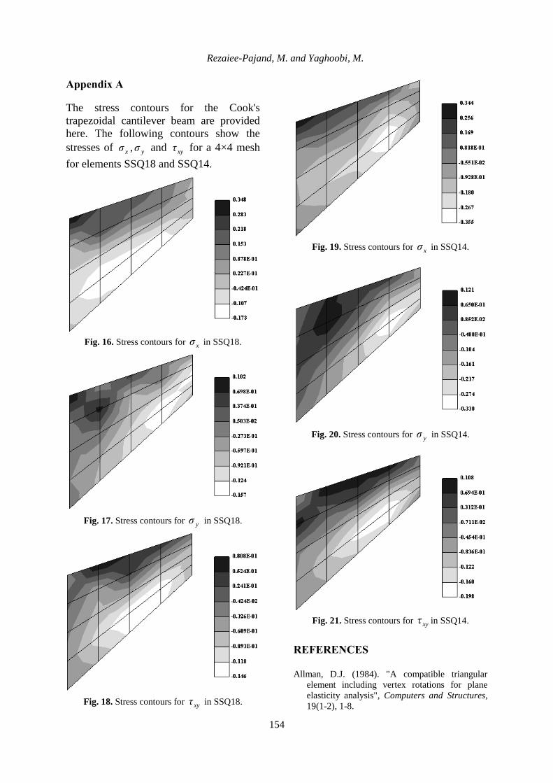
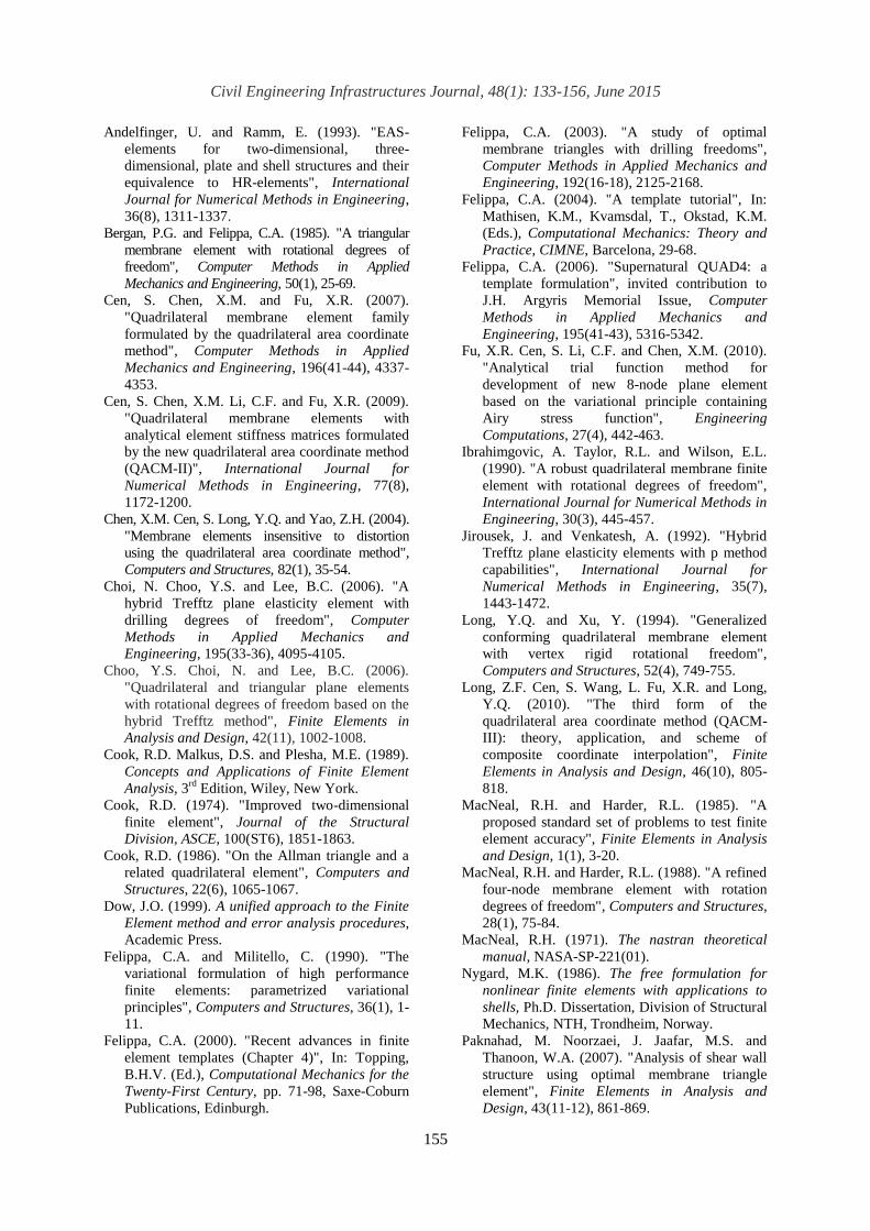
Appendix A
The stress contours for the Cook's
trapezoidal cantilever beam are provided
here. The following contours show the
stresses of xσ , yσ and xyτ for a 4×4 mesh
for elements SSQ18 and SSQ14.
Fig. 16. Stress contours for xσ in SSQ18.
Fig. 17. Stress contours for yσ in SSQ18.
Fig. 18. Stress contours for xyτ in SSQ18.
Fig. 19. Stress contours for xσ in SSQ14.
Fig. 20. Stress contours for yσ in SSQ14.
Fig. 21. Stress contours for xyτ in SSQ14.
REFERENCES
Allman, D.J. (1984). "A compatible triangular
element including vertex rotations for plane
elasticity analysis", Computers and Structures,
19(1-2), 1-8.
Civil Engineering Infrastructures Journal, 48(1): 133-156, June 2015
155
Andelfinger, U. and Ramm, E. (1993). "EAS-
elements for two-dimensional, three-
dimensional, plate and shell structures and their
equivalence to HR-elements", International
Journal for Numerical Methods in Engineering,
36(8), 1311-1337.
Bergan, P.G. and Felippa, C.A. (1985). "A triangular
membrane element with rotational degrees of
freedom", Computer Methods in Applied
Mechanics and Engineering, 50(1), 25-69.
Cen, S. Chen, X.M. and Fu, X.R. (2007).
"Quadrilateral membrane element family
formulated by the quadrilateral area coordinate
method", Computer Methods in Applied
Mechanics and Engineering, 196(41-44), 4337-
4353.
Cen, S. Chen, X.M. Li, C.F. and Fu, X.R. (2009).
"Quadrilateral membrane elements with
analytical element stiffness matrices formulated
by the new quadrilateral area coordinate method
(QACM-II)", International Journal for
Numerical Methods in Engineering, 77(8),
1172-1200.
Chen, X.M. Cen, S. Long, Y.Q. and Yao, Z.H. (2004).
"Membrane elements insensitive to distortion
using the quadrilateral area coordinate method",
Computers and Structures, 82(1), 35-54.
Choi, N. Choo, Y.S. and Lee, B.C. (2006). "A
hybrid Trefftz plane elasticity element with
drilling degrees of freedom", Computer
Methods in Applied Mechanics and
Engineering, 195(33-36), 4095-4105.
Choo, Y.S. Choi, N. and Lee, B.C. (2006).
"Quadrilateral and triangular plane elements
with rotational degrees of freedom based on the
hybrid Trefftz method", Finite Elements in
Analysis and Design, 42(11), 1002-1008.
Cook, R.D. Malkus, D.S. and Plesha, M.E. (1989).
Concepts and Applications of Finite Element
Analysis, 3rd
Edition, Wiley, New York.
Cook, R.D. (1974). "Improved two-dimensional
finite element", Journal of the Structural
Division, ASCE, 100(ST6), 1851-1863.
Cook, R.D. (1986). "On the Allman triangle and a
related quadrilateral element", Computers and
Structures, 22(6), 1065-1067.
Dow, J.O. (1999). A unified approach to the Finite
Element method and error analysis procedures,
Academic Press.
Felippa, C.A. and Militello, C. (1990). "The
variational formulation of high performance
finite elements: parametrized variational
principles", Computers and Structures, 36(1), 1-
11.
Felippa, C.A. (2000). "Recent advances in finite
element templates (Chapter 4)", In: Topping,
B.H.V. (Ed.), Computational Mechanics for the
Twenty-First Century, pp. 71-98, Saxe-Coburn
Publications, Edinburgh.
Felippa, C.A. (2003). "A study of optimal
membrane triangles with drilling freedoms",
Computer Methods in Applied Mechanics and
Engineering, 192(16-18), 2125-2168.
Felippa, C.A. (2004). "A template tutorial", In:
Mathisen, K.M., Kvamsdal, T., Okstad, K.M.
(Eds.), Computational Mechanics: Theory and
Practice, CIMNE, Barcelona, 29-68.
Felippa, C.A. (2006). "Supernatural QUAD4: a
template formulation", invited contribution to
J.H. Argyris Memorial Issue, Computer
Methods in Applied Mechanics and
Engineering, 195(41-43), 5316-5342.
Fu, X.R. Cen, S. Li, C.F. and Chen, X.M. (2010).
"Analytical trial function method for
development of new 8-node plane element
based on the variational principle containing
Airy stress function", Engineering
Computations, 27(4), 442-463.
Ibrahimgovic, A. Taylor, R.L. and Wilson, E.L.
(1990). "A robust quadrilateral membrane finite
element with rotational degrees of freedom",
International Journal for Numerical Methods in
Engineering, 30(3), 445-457.
Jirousek, J. and Venkatesh, A. (1992). "Hybrid
Trefftz plane elasticity elements with p method
capabilities", International Journal for
Numerical Methods in Engineering, 35(7),
1443-1472.
Long, Y.Q. and Xu, Y. (1994). "Generalized
conforming quadrilateral membrane element
with vertex rigid rotational freedom",
Computers and Structures, 52(4), 749-755.
Long, Z.F. Cen, S. Wang, L. Fu, X.R. and Long,
Y.Q. (2010). "The third form of the
quadrilateral area coordinate method (QACM-
III): theory, application, and scheme of
composite coordinate interpolation", Finite
Elements in Analysis and Design, 46(10), 805-
818.
MacNeal, R.H. and Harder, R.L. (1985). "A
proposed standard set of problems to test finite
element accuracy", Finite Elements in Analysis
and Design, 1(1), 3-20.
MacNeal, R.H. and Harder, R.L. (1988). "A refined
four-node membrane element with rotation
degrees of freedom", Computers and Structures,
28(1), 75-84.
MacNeal, R.H. (1971). The nastran theoretical
manual, NASA-SP-221(01).
Nygard, M.K. (1986). The free formulation for
nonlinear finite elements with applications to
shells, Ph.D. Dissertation, Division of Structural
Mechanics, NTH, Trondheim, Norway.
Paknahad, M. Noorzaei, J. Jaafar, M.S. and
Thanoon, W.A. (2007). "Analysis of shear wall
structure using optimal membrane triangle
element", Finite Elements in Analysis and
Design, 43(11-12), 861-869.
Rezaiee-Pajand, M. and Yaghoobi, M.
156
Pian, T.H.H. and Sumihara, K. (1984). "Rational
approach for assumed stress finite elements",
International Journal for Numerical Methods in
Engineering, 20(9), 1685-1695.
Piltner, R. and Taylor, R.L. (1995). "A quadrilateral
mixed finite element with two enhanced strain
modes", International Journal for Numerical
Methods in Engineering, 38(11), 1783-1808.
Piltner, R. and Taylor, R.L. (1997). "A systematic
constructions of B-bar functions for linear and
nonlinear mixed-enhanced finite elements for
plane elasticity problems", International
Journal for Numerical Methods in Engineering,
44(5), 615-639.
Prathap, G. and Senthilkumar, V. (2008). "Making
sense of the quadrilateral area coordinate
membrane elements", Computer Methods in
Applied Mechanics and Engineering, 197(49-
50), 4379-4382.
Rezaiee-Pajand, M. and Yaghoobi, M. (2012).
"Formulating an effective generalized four-
sided element", European Journal of Mechanics
A/Solids, 36, 141-155.
Santos, H.A.F.A. and Moitinho de Almeida, J.P.
(2014). "A family of Piola–Kirchhoff hybrid
stress finite elements for two-dimensional linear
elasticity", Finite Elements in Analysis and
Design, 85, 33–49.
Taylor, R.L. Beresford, P.J. and Wilson, E.L.
(1976). "A non-conforming element for stress
analysis", International Journal for Numerical
Methods in Engineering, 10(6), 1211-1219.
Wilson, E.L. Taylor, R.L. Doherty, W.P. and
Ghabussi, T. (1973). "Incompatible
displacement models", In: Fenven, S.T., et al.
(Eds.), Numerical and Computer Methods in
Structural Mechanics, pp. 43-57, Academic
Press, New York.
Wisniewski, K. and Turska, E. (2006). "Enhanced
Allman quadrilateral for finite drilling
Rotations", Computer Methods in Applied
Mechanics and Engineering, 195(44-47), 6086-
6109.
Wisniewski, K. and Turska, E. (2008). "Improved
four-node Hellingere Reissner elements based
on skew coordinates", International Journal for
Numerical Methods in Engineering, 76(6), 798-
836.
Wisniewski, K. and Turska, E. (2009). "Improved
4-node Hu-Washizu elements based on skew
coordinates", Computers and Structures, 87(7-
8), 407-424.
Wu, C.C. Huang, M.G. and Pian, T.H.H. (1987).
"Consistency condition and convergence criteria
of incompatible elements: general formulation
of incompatible functions and its application",
Computers and Structures, 27(5), 639-644.
Yeo, S.T. and Lee, B.C. (1997). "New stress
assumption for hybrid stress elements and
refined four-node plane and eight-node brick
elements", International Journal for Numerical
Methods in Engineering, 40(16), 2933-2952.


