

Two Sample Hypothesis Testing for Functional Data
Gina-Maria Pomann, Ana-Maria Staicu*, Sujit Ghosh
Department of Statistics, North Carolina State University, SAS Hall, 2311 Stinson Drive,Raleigh, NC USA 27695-8203
Abstract
A nonparametric testing procedure is proposed for testing the hypothesis that
two samples of curves observed at discrete grids and with noise have the same
underlying distribution. Our method relies on representing the curves using a
common orthogonal basis expansion. The approach reduces the dimension of
the testing problem in a way that enables the application of traditional non-
parametric univariate testing procedures. This procedure is computationally
inexpensive, can be easily implemented, and accommodates different sampling
designs across the samples. Numerical studies confirm the size and power prop-
erties of the test in many realistic scenarios, and furthermore show that the
proposed test is more powerful than alternative testing procedures. The pro-
posed methodology is illustrated on a state-of-the art diffusion tensor imaging
study, where the objective is to compare white matter tract profiles in healthy
individuals and multiple sclerosis patients.
Keywords: Anderson Darling test, Diffusion tensor imaging, Functional data,
Functional principal component analysis, Hypothesis testing, Multiple Sclerosis
1. Introduction
Statistical inference in functional data analysis has been under intense method-
ological and theoretical development, especially due to the explosion of applica-
tions involving data with functional features; see Besse & Ramsay (1986), Rice
URL: *Email corresponding author: [email protected] (Ana-Maria Staicu*)
Preprint submitted to Journal of LATEX Templates March 5, 2014

& Silverman (1991), Ramsay & Silverman (2005), Ferraty et al. (2007), and5
Horvath & Kokoszka (2012) to name a few. Nevertheless, testing the hypothe-
sis that the generating distributions of two sets of curves are identical, when the
observed data are noisy and discrete realizations of the curves, has received very
little attention. Furthermore, there are no formal procedures openly available to
investigate this hypothesis testing. In this paper, we propose a novel framework10
to address this testing problem, and provide an easy-to-use software implemen-
tation. Our approach is applicable to a variety of realistic scenarios, such as 1)
curves observed at dense or sparse grids of points, with or without measurement
error, 2) different sampling designs across the samples, and 3) different sample
sizes. The methodology scales well with the total sample size, and it can be15
extended to test for the equality of more than two samples of curves. Our mo-
tivating application is a brain tractography study, where the objective to assess
if certain imaging modalities are useful in differentiating between patients with
multiple sclerosis (MS) and healthy controls. In particular, the interest is to
assess whether the parallel diffusivity or fractional anisotropy along the corpus20
callosum - the largest identified white matter tract - have identical distribution
in MS patients and healthy controls.
Two sample hypothesis testing for functional data has been approached in
many contexts; ranging from testing for specific types of differences, such as
differences in the mean or covariance functions, to testing for overall differences25
in the cumulative density functions. To detect differences in the mean functions
of two independent samples of curves, Ramsay & Silverman (2005) introduced a
pointwise t-test, Zhang et al. (2010) presented an L2−norm based test, Horvath
et al. (2013) proposed a test based on the sample means of the curves, and Staicu
et al. (2014) developed a pseudo likelihood ratio test. Extension to k indepen-30
dent samples of curves was discussed in Cuevas et al. (2004), Estevez-Perez &
Vilar (2008), and Laukaitis & Rackauskas (2005), who proposed ANOVA-like
testing procedures for testing the equality of mean functions. Recent research
also focused on detecting differences in the covariance functions of independent
samples of curves: see the factor-based test proposed by Ferraty et al. (2007),35
2

the regularized M-test introduced by Kraus & Panaretos (2012), and the chi-
squared test proposed by Fremdt et al. (2012).
Literature on testing the equality of the distribution of two samples of func-
tional data observed at discrete grid points and possibly with error is rather
scarce and has been considered previously only by Hall & Van Keilegom (2007).40
The authors proposed a Cramer-von Mises (CVM) - type of test, based on
the empirical distributional functionals of the reconstructed smooth trajecto-
ries, when functional data are observed on dense designs. Benko et al. (2009)
attempts to address this testing problem by first using a functional principal
components (FPC) decomposition of the data and then employing a sequen-45
tial bootstrap test to identify differences in the mean functions, eigenfunctions,
and eigenvalues. However, in the proposed form, this test does not account for
multiple comparisons and is difficult to study under a variety of scenarios due
to its computational expense. Furthermore, even if the multiple comparisons
are properly accounted for, the test is still limited to detecting first and second50
order changes in the distribution of the FPC scores.
In this paper, we propose an approach based on functional principal com-
ponents analysis and the Karhunen-Loeve (KL) representation of the combined
data. By representing the data using an overall eigenbasis, we are able to reduce
the original two-sample functional testing problem to an approximate simpler55
finite dimensional testing problem. The methodology is illustrated using the
two-sample Anderson-Darling statistic (Pettitt, 1976); however, any other two-
sample tests can also be used. Our simulation results show that in cases where
the approach of Hall & Van Keilegom (2007) applies, our proposed test is con-
siderably more powerful.60
The rest of the paper is structured as follows. Section 2 describes the sta-
tistical framework and the testing procedure when the true curves are observed
entirely and without noise. Section 3 discusses the approach when the observed
data consist of noisy and discrete realizations of some underlying curves for
dense as well as sparse sampling designs. In Section 4 we evaluate numerically65
the size and power of the proposed methodology in a simulation experiment.
3

The methodology is then applied to the brain tractography data in Section 5.
The paper concludes with a brief discussion in Section 6.
2. Two Sample Testing for Functional Data
2.1. Preliminary70
Suppose we observe data arising from two groups, [Y1ij , t1ij : i ∈ {1, . . . , n1} and j ∈
{1, . . . ,m1i}] and [Y2ij , t2ij : i ∈ {1, . . . , n2} and j ∈ {1, . . . ,m2i}], where t1ij , t2ij ∈
T for some bounded and closed interval T; for simplicity take T = [0, 1]. The
notation of the time-points, t1ij and t2ij , allows for different observation points
in the two groups. It is assumed that the Y1ij ’s and Y2ij ’s are independent
realizations of two underlying processes observed with noise on a finite grid of
points. Specifically, consider
Y1ij = X1i(t1ij) + ε1ij , and Y2ij = X2i(t2ij) + ε2ij , (1)
whereX1i(·)iid∼ X1(·) andX2i(·)
iid∼ X2(·) are independent and square-integrable
random functions over T, for some underlying random processes X1(·) and X2(·).
It is assumed that X1(·) and X2(·) have unknown continuous mean and contin-
uous and positive semi-definite covariance functions. The measurement errors,
{ε1ij}i,j and {ε2ij}i,j , are independent and identically distributed with mean
zero, and with variances σ2ε1 and σ2
ε2 respectively, and are independent of X1i(·)
and X2i(·). Our objective is to test the null hypothesis,
H0 : X1(·) d= X2(·) (2)
versus the alternative hypothesis HA : X1(·)d
6= X2(·), where “d=” means that the
processes on either side have the same distribution. In particular our interest is
to develop non-parametric and computationally inexpensive methods for testing
this hypothesis.
Since X1(·) and X2(·) are processes defined over a continuum, testing (2)75
implies testing the null hypothesis that two infinite dimensional objects have
4

the same generating distribution. This is different from two sample testing in a
multivariate framework, where the dimension of the random objects of interest
is finite. In the case where the sampling design is common to all the subjects
(i.e. t1ij = t2ij = tj and m1i = m2i = m), the dimension of the testing problem80
could potentially be reduced by testing an approximate null hypothesis - that
the multivariate distribution of the processes evaluated at the observed grid
points are equal. Multivariate testing procedures (eg. Aslan & Zech (2005);
Friedman & Rafsky (1979); Read & Cressie (1988)) could be employed in this
situation. However, these procedures have only been illustrated for cases when85
m = 4 or 5 in our notation. In dense functional data, the number of unique
time-points, m, is orders of magnitude larger, often even larger than the sample
size.
Recent research has approached this problem using functional data analysis
based techniques. For example Hall & Van Keilegom (2007) propose an exten-90
sion of the Cramer-von Mises (CVM) test from multivariate statistics, and use
bootstrap to approximate the null distribution of the test. Benko et al. (2009)
consider a common functional principal components model for the two samples
and proposed bootstrap procedures to test for the equality of the corresponding
model components. Both approaches rely on bootstrap techniques which makes95
it unfeasible to perform sufficient empirical power analysis when the sample
sizes are large.
We propose a novel approach for the hypothesis testing (2) that relies on
modeling the data using FPC analysis and on functional principal component
analysis (FPCA) of the overall data and on common multivariate testing pro-100
cedures. Our methodology is based on basis functions representation of the
data using the overall eigenbasis, which facilitates dimension reduction of the
functional objects. This allows simplification of the hypothesis testing (2) to
two-sample multivariate testing of the equality of the distributions of the basis
coefficients. Furthermore, we reduce the testing (2) to a sequence of two-sample105
tests for the equality of univariate distributions combined with a multiple testing
correction. The proposed procedure is computationally inexpensive and scales
5

well with large sample sizes.
2.2. Testing Procedure
To begin with, we describe the methodology under the assumption that the110
curves are observed entirely and without noise (Hall et al., 2006). Extension
to practical settings is discussed in Section 3. Consider two sets of indepen-
dent curves {X1l(·), . . . , X1n1(·)} and {X21(·), . . . , X2n2
(·)} , defined on [0, 1].
Assume X1i(·) ∼ X1(·) and X2i(·) ∼ X2(·) are square integrable and have con-
tinuous mean and covariance functions respectively. This section develops a115
testing procedure for testing the null hypothesis (2).
Our methodology is developed under the assumption that both n1, n2 →∞
such that limn1,n2→∞ n1/(n1 + n2) = p ∈ (0, 1). Let X(·) be the mixture pro-
cess of X1(·) and X2(·) with mixture probabilities p and 1 − p respectively.
Let Z be a binary random variable that takes values one and two such that120
P (Z = 1) = p. Then X1(·) is the conditional process X(·) given Z = 1, and
X2(·) is the conditional process X(·) given Z = 2. It follows that X(·) is square
integrable, has continuous mean and positive semi-definite covariance functions.
Let µ(t) = E[X(t)] be the mean function and let Σ(t, s) = cov{X(t), X(s)} be
the covariance function. Mercer’s theorem yields the spectral decomposition of125
the covariance function, Σ(t, s) =∑k≥1 λkφk(t)φk(s) in terms of non-negative
eigenvalues λ1 ≥ λ2 ≥ . . . ≥ 0 and orthogonal eigenfunctions φk(·), with∫ 1
0φk(t)φk′(t)dt = 1(k = k′), where 1(k = k′) is the indicator function which is
1 when k = k′ and 0 otherwise (Bosq, 2000). The decomposition implies that
X(·) can be represented via the KL expansion as X(t) = µ(t) +∑∞k=1 ξkφk(t)130
where ξk =∫ 1
0{X(t)−µ(t)}φk(t)dt are commonly called FPC scores and are as-
sumed to be uncorrelated random variables with zero mean and variance equal
to λk. For practical as well as theoretical reasons (see for example Yao et al.
(2005), Hall et al. (2006), or Di et al. (2009)) the infinite expansion of X(·) is
often truncated. Let XK(t) = µ(t) +∑Kk=1 ξkφk(t) be the truncated KL expan-135
sion of X(·). It follows that XK(t)→ X(t) as K →∞, where the convergence
is in quadratic mean.
6

Assumption (A): Let ξzk =∫ 1
0(Xz(t)− µ(t))φk(t)dt for k ≥ 1 and z = 1, 2.
Assume that E[{Xz(t) − µ(t) −∑Kk=1 ξzkφk(t)}2] → 0 for K → ∞, uniformly
in t, and for z ∈ {1, 2}.140
This assumption is satisfied if both processes X1(t) and X2(t) are modeled
using the common FPC model discussed in Benko et al. (2009), which assumes
common mean function and common eigenfunctions. However, condition (A) is
much weaker than the common functional principal component model; one can
easily construct examples where Xz(t) has eigenfunctions that differ for z = 1145
and z = 2 and still satisfy (A). An equivalent way to write condition (A) is
Xz(t) = µ(t) +∑∞k=1 ξzkφk(t), for z = 1, 2. Remark that ξzk do not necessarily
have zero mean nor are uncorrelated over k; in fact they may have mean and
variance that depend on z. In the remaining of the paper we refer to ξzk by
basis coefficients. This model assumption has been considered in the literature150
of functional data analysis, but mainly from modeling perspectives (Chiou et al.,
2003; Aston et al., 2010).
Let XKz (t) = µ(t) +
∑Kk=1 ξzkφk(t) be a finite-dimensional approximation
of Xz(t). We note that assumption (A) states that XKz (t) → Xz(t) in mean
squared error as K →∞. Furthermore, if the null hypothesis, H0 in (2), holds155
true then it follows that XK1 (·) d
= XK2 (·), for each finite truncation K. Let K
be a suitable finite-dimensional truncation such that XK(·) approximates X(·)
sufficiently accurate using L2 norm; it follows that XKz (·) approximates well
Xz(·) for z = 1, 2.
Proposition: Assume condition A holds. Then the null hypothesis (2) can be160
reduced to
HK0 : {ξzk}Kk=1
d= {ξzk}Kk=1, (3)
where the notation HK0 is to emphasize the dependence of the reduced null
hypothesis on the finite truncation K.
The proof of this result is based on the observation that for finite truncation
K, we have XK1 (·) d
= XK2 (·) if only if the multivariate distributions of basis165
7
coefficients, {ξ1k}Kk=1 and {ξ2k}Kk=1, are the same.
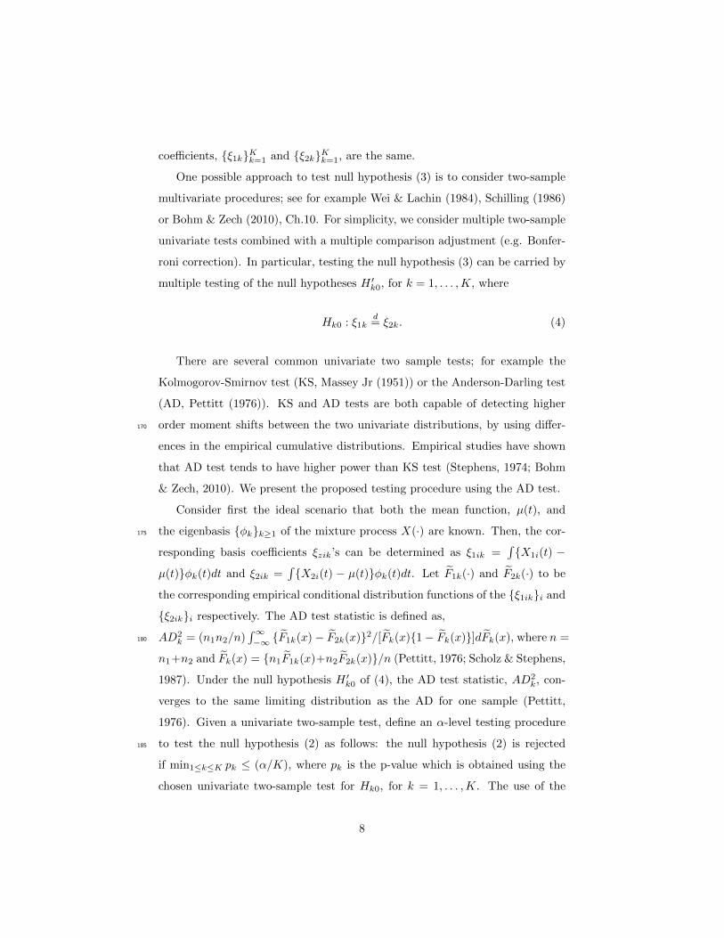
One possible approach to test null hypothesis (3) is to consider two-sample
multivariate procedures; see for example Wei & Lachin (1984), Schilling (1986)
or Bohm & Zech (2010), Ch.10. For simplicity, we consider multiple two-sample
univariate tests combined with a multiple comparison adjustment (e.g. Bonfer-
roni correction). In particular, testing the null hypothesis (3) can be carried by
multiple testing of the null hypotheses H ′k0, for k = 1, . . . ,K, where
Hk0 : ξ1kd= ξ2k. (4)
There are several common univariate two sample tests; for example the
Kolmogorov-Smirnov test (KS, Massey Jr (1951)) or the Anderson-Darling test
(AD, Pettitt (1976)). KS and AD tests are both capable of detecting higher
order moment shifts between the two univariate distributions, by using differ-170
ences in the empirical cumulative distributions. Empirical studies have shown
that AD test tends to have higher power than KS test (Stephens, 1974; Bohm
& Zech, 2010). We present the proposed testing procedure using the AD test.
Consider first the ideal scenario that both the mean function, µ(t), and
the eigenbasis {φk}k≥1 of the mixture process X(·) are known. Then, the cor-175
responding basis coefficients ξzik’s can be determined as ξ1ik =∫{X1i(t) −
µ(t)}φk(t)dt and ξ2ik =∫{X2i(t) − µ(t)}φk(t)dt. Let F1k(·) and F2k(·) to be
the corresponding empirical conditional distribution functions of the {ξ1ik}i and
{ξ2ik}i respectively. The AD test statistic is defined as,
AD2k = (n1n2/n)
∫∞−∞ {F1k(x)− F2k(x)}2/[Fk(x){1− Fk(x)}]dFk(x), where n =180
n1+n2 and Fk(x) = {n1F1k(x)+n2F2k(x)}/n (Pettitt, 1976; Scholz & Stephens,
1987). Under the null hypothesis H ′k0 of (4), the AD test statistic, AD2k, con-
verges to the same limiting distribution as the AD for one sample (Pettitt,
1976). Given a univariate two-sample test, define an α-level testing procedure
to test the null hypothesis (2) as follows: the null hypothesis (2) is rejected185
if min1≤k≤K pk ≤ (α/K), where pk is the p-value which is obtained using the
chosen univariate two-sample test for Hk0, for k = 1, . . . ,K. The use of the
8

Bonferroni correction ensures that the testing procedure maintains its nominal
size, conditional on the truncation level K. Because we apply it to functional
data we call this test the Functional Anderson-Darling (FAD). The proposed190
testing methodology allows us to extend any univariate testing to the case of
functional data. Of course, any advantages or drawbacks of the univariate tests
- such as the ability to detect higher order moment shifts or weak power in small
sample sizes - will carry over to the functional extension.
Finally consider the more typical scenario where the mean and eigenbasis are195
not known and require to be estimated. Let µ(·) and Σ(·, ·) be the sample mean
and the sample covariance of the entire set of curves, {X1i(·) : i = 1, . . . , n1}
and {X2i(·) : i = 1, . . . , n2}, respectively. Furthermore let {λk, φk(·)}k≥1 be
the pair of the estimated eigenvalues/eigenfunctions of the spectral decom-
position of Σ(·, ·). As before, let ξ1ik =∫{X1i(t) − µ(t)}φk(t)dt and ξ2ik =200 ∫
{X2i(t)− µ(t)}φk(t)dt be the estimated basis coefficients of X1i(·) and X2i(·)
respectively. Moreover, define by AD2
k the statistic analogous to AD2k, with
the basis coefficients ξ1ik and ξ2ik replacing ξ1ik and ξ2ik, respectively. If con-
dition (A) is valid, then we conjecture that if the null hypothesis Hk0 (4) is
true, then the asymptotic distribution of AD2
k is the same as the asymptotic205
null distribution of AD2k.
3. Extension to Practical Situations
Using the testing procedure described in Section 2.2 is not straightforward
in practical applications, as the true smooth trajectories Xi(·) and thus the true
scores ξik are not directly observable. Instead the observed data are {Y1ij : 1 ≤210
i ≤ n1, 1 ≤ j ≤ m1i} and {Y2ij : 1 ≤ i ≤ n2, 1 ≤ j ≤ m2i}, as described in
model (1). Let Zi be the variable that denotes the group membership of the ith
curve. To address this challenge, we propose to replace ξzik from the previous
section by appropriate estimators, ξzik, and thus test the hypotheses H0k in (4)
using ξzik’s instead of ξzik’s for z = 1, 2.215
Intuitively, our logic is based on the result that under null hypothesis (2)
9

ξ1ik − ξ2ikp→ 0 as n → ∞ where “
p→” denotes convergence in probability,
for k = 1, . . . ,K. Thus, to test (4) one can use the proposed testing procedure
described in the previous section, but with the estimated basis coefficients ξ1ik’s
and ξ2ik respectively, instead of the true ones.220
3.0.1. Dense design
First, consider the situation when the grid of points for each subject is dense
in [0, 1], that is m1i and m2i are very large. Zhang & Chen (2007) proved that
one can reconstruct the curves Xi(t) with negligible error by smoothing the ob-
served functional observations {Yij}m1ij=1 using local polynomial kernel smooth-225
ing. Let X1i(·) and X2i(·) be the reconstructed trajectories in group one and two
respectively. The main requirement for such reconstruction is that the number
of measurements m1i and m2i for all subjects tends to infinity at a rate faster
than the sample sizes n1, and n2 respectively.
Consider the pooled sample {X1i(·) : i = 1, . . . , n1}∪{X2i(·) : i = 1, . . . , n2}230
and denote by Xi(t) a generic curve in this sample. Let µ(t) be the sample aver-
age and let Σ(t, s) be the sample covariance functions of the reconstructed tra-
jectories Xi(t). Under regularity assumptions these functions are asymptotically
identical to the ideal estimators based on the true trajectories (Zhang & Chen,
2007). The spectral decomposition of the covariance function yields the pairs of235
estimated eigenfunctions and eigenvalues {φk(t), λk}k, with λ1 > λ2 > . . . ≥ 0.
It follows that ξik =∫{Xi(t) − µ(t)}φk(t)dt are consistent estimators of the
FPC scores ξik (Hall et al., 2006; Zhang & Chen, 2007); ξ1ik = ξik if Zi = 1
and ξ2ik = ξik if Zi = 2. Therefore, for large sample sizes n1 and n2, the distri-
bution of ξzik approximates that of ξzik. In applications, ξik can be calculated240
via numerical integration. Therefore, ξik are used for testing the null hypoth-
esis (3). The finite truncation K of the estimated eigenfunctions {φk(t)}k can
be chosen using model selection based-criteria. We found that the cumulative
explained variance criterion (Di et al., 2009; Staicu et al., 2010) works very well,
for estimation of K, in practice.245
10

3.0.2. Sparse design
Next consider the situation when the grid of points for each subject is dense
in [0, 1], however, m1i,m2i <∞ and possibly small. The sparse setting requires
different methodology for several reasons. First, the bounding constraint on the
number of repeated observations, m1i, and m2i respectively, implies a sparse250
setting at the curve level and does not provide accurate estimators by smoothing
each curve separately. Secondly, estimation of the basis coefficients ξik via
numerical integration is no longer reliable. Instead, we consider the pooled
sample {Y1ij : i, j} ∪ {Y2ij : i, j}, and let [Yij : j ∈ {1, . . .mi}] be a generic
observed profile in this set. The observed measurements [Yij : j ∈ {1, . . .mi}]i255
are viewed as independent and identically distributed realizations of a stochastic
process, that are observed at finite grids {ti1, . . . , timi} and contaminated with
error. Specifically it is implied that Yij = Xi(tij) + εij , for Xi(·) which is a
process as described earlier with E[X(t)] = µ(t) and cov{X(t), X(s)} = Σ(t, s).
Here εij ’s are independent and identically distributed measurement error with260
zero mean and variance σ2.
Common FPCA-techniques can be applied to reconstruct the underlying
subject-trajectories, Xi(·) from the observed data {Yij : 1 ≤ j ≤ mi} (Yao et al.,
2005; Di et al., 2009). The key idea is to first obtain estimates of the smooth
mean and covariance functions, µ(t) and Σ(t, s) respectively. The spectral de-265
composition of the estimated covariance yields the eigenfunction/eigenvalue
pairs, {φk(·), λk}k≥1, where λ1 > λ2 > . . . ≥ 0. Next, the variance of the
noise is estimated based on the difference between the pointwise variance of the
observed data Yij ’s and the estimated pointwise variance Σ(t, t) (Staniswalis &
Lee, 1998; Yao et al., 2005). There are several ways in the literature to select (or270
estimate) the finite truncation K, such as Akaike Information Criterion (AIC),
Bayesian Information Criterion (BIC) etc.; from our empirical experience the
simple criterion based on percentage of explained variance (such as 90% or 95%)
gives satisfactory results. In our simulation experiments we use the cumulative
explained variance to select K. Sensitivity with regards to this parameter is275
11

studied in Section 4.
Once the mean function, eigenfunctions, eigenvalues, and noise variance
are estimated, the model for the observed data {Yij : 1 ≤ j ≤ mi}i be-
comes a linear mixed effects model Yij = µ(tij) +∑k ξikφk(tij) + εij , where
var(ξik) = λk and var(εij) = σ2. The coefficients ξik can be predicted us-280
ing the conditional expectation formula ξik = E[ξik|(Yi1, . . . , Yimi)]. Under
the assumption that the responses and errors are jointly Gaussian, the pre-
dicted coefficients are in fact the empirical best linear unbiased predictors:
ξik = λkΦTi (Σi + σ2Imi×mi)−1(Yi − µi). Here Yi is the mi-dimensional vec-
tor of Yij , µi and Φi are mi-dimensional vectors with the jth entries µ(tij) and285
φ(tij) respectively, Σi is a mi × mi-dimensional matrix with the (j, j′)th en-
try equal to Σ(tij , tij′), and Imi×miis the mi ×mi identity matrix. Yao et al.
(2005) proved that ξik’s are consistent estimators of ξik = E[ξik|(Yi1, . . . , Yimi)].
Define ξzik = ξik when Zi = z and similarly define ξzik = ξik if Zi = z. Then,
under the joint Gaussian assumption we have that ξ1ikp= ξ2ik is equivalent to290
ξ1ikp= ξ2ik for k = 1, . . . ,K. It follows that for large sample sizes n1 and n2
the sampling distribution of ξ1ik’s and ξ2ik’s are the same as those of ξ1ik’s and
ξ2ik’s, respectively. Therefore we can use ξzik’s to test the null hypothesis (4).
4. Simulation Studies
We present now the performance of the proposed testing procedure, under a295
variety of settings and for varying sample sizes. Section 4.1 studies Type I error
rate of the FAD test and the sensitivity to the percentage of explained variance,
τ , used to determine the truncation parameter, K. Additionally, it investigates
the empirical power in various scenarios. Sections 4.2 compares numerically the
proposed approach with the closest available competitor - the Cramer-von Mises300
(CVM) -type test introduced by Hall & Van Keilegom (2007).
4.1. Type One Error and Power Performance
We construct datasets {(t1ij , Y1ij) : j}n1i=1 and {(t2ij , Y2ij) : j}n2
i=1 using
model (1) for t1ij = t2ij = tj observed on an equally spaced grid of m = 100
12

points in [0, 1]. Here X1i(t) = µ1(t) +∑k φk(t)ξ1ik and X2i(t) = µ2(t) +305 ∑
k φk(t)ξ2ik, where φ1(t) =√
2 sin(2πt), φ2(t) =√
2 cos(2πt) and so on, are
the Fourier basis functions, ξ1ik and ξ2ik are uncorrelated respectively with
var(ξ1ik) = λ1k, var(ξ2ik) = λ2k and λ1k = λ2k = 0 for k ≥ 4. We set
ε1ij ∼ N(0, 0.25) and ε2ij ∼ N(0, 0.25). The design corresponds to a common
functional principal component model (see Benko et al. (2009)), since the two310
sets of curves have the same eigenbasis, {φk}k; the coefficients ξ1ik and ξ2ik
are the corresponding functional principal component scores. Nevertheless, the
mean functions are allowed to be different for the two groups of curves.
The FAD test is employed to test the null hypothesis (2); the mean functions,
the overall basis functions, and corresponding basis coefficients are estimated315
using the methods described in Section 3. The number of basis functions is
selected using the percentage of explained variance, τ , for the pooled data. We
use τ = 95% in our simulation experiments; as we illustrate next the FAD test is
robust to this parameter. The estimates for all the model components, including
the basis coefficients, are obtained using the R package refund (Crainiceanu320
et al., 2012). Next, the R package AD (Scholz, 2011) is used to test the equality
of the corresponding univariate distributions for each pair of basis coefficients.
The Bonferroni multiple testing correction is used to maintain the desired level
of the FAD test. The null hypothesis is rejected/not rejected according to the
approach described in Section 2.2. All the results in this section are based on325
α = 0.05 significance level.
First, we assess the Type I error rate for various threshold parameter values,
τ . For simplicity set µ1(t) = µ2(t) = 0 for all t and consider ξ1ik, ξ2ik ∼
N(0, λk), for λ1 = 10, λ2 = 5, and λ3 = 2. Type I error rate is studied
for varying τ from 80% to 99% and for increasing equal/unequal sample sizes.330
When τ = 80%, the proposed criterion to select the number of eigenfunctions
yields K = 2 eigenfunctions as being sufficient to explain 80% of the variability,
while when τ = 99% the criterion yields K = 3 eigenfunctions. Table 1 displays
the empirical size of the FAD test using varying thresholds τ for the case when
the sample size is equal or unequal, with an overall size increasing from 200335
13

to 2000. The results are based on 5000 MC replications. They show that, as
expected, the size of the test is not too sensitive to the threshold τ ; the size is
close to the nominal level α = 0.05 in all cases. Additionally, we investigated
numerically the effect of the threshold on the power capabilities, and found that
it has very little effect on the power (results not reported).340
PPPPPPPP(n1, n2)
τ0.80 0.85 0.90 0.95 0.99
(100,100) 0.056 0.056 0.059 0.060 0.060(200,200) 0.050 0.050 0.052 0.053 0.053(300,300) 0.053 0.053 0.049 0.049 0.049(500,500) 0.049 0.049 0.050 0.050 0.050
(1000,1000) 0.055 0.055 0.058 0.058 0.058(50,150) 0.055 0.055 0.058 0.058 0.057(100,300) 0.053 0.053 0.049 0.049 0.049(150,450) 0.048 0.048 0.055 0.054 0.054(250,750) 0.051 0.051 0.054 0.054 0.054(500,1500) 0.055 0.055 0.053 0.053 0.053
Table 1: Estimated Type I Error rate of FAD test, based on 5000 replications,for different threshold values τ . Displayed are results for equal and unequalsample sizes, n1, n2.
Next, we study the power performance of the FAD test with τ = 0.95.
The distribution of the true processes is described by the mean functions, as
well as by the distributions of the basis coefficients. The following scenarios
refer to cases where the distributions differ at various orders of the moments of
the coefficient distributions. Setting A corresponds to deviations in the mean345
functions, settings B and C correspond to deviations in the second moment and
third moment, respectively of the corresponding distribution of the first set of
basis coefficients. Throughout this section it is assumed that λ1k = λ2k = 0 for
all k ≥ 3.
A Mean Shift: Set the mean functions as µ1(t) = t and µ2(t) = t + δt3.350
Generate the coefficients as ξ1i1, ξ2i1 ∼ N(0, 10), ξ1i2, ξ2i2 ∼ N(0, 5). The
index δ controls the departure in the mean behavior of the two distribu-
tions.
14

B Variance Shift: Set µ1(t) = µ2(t) = 0. Generate the coefficients ξ1i1 ∼
N(0, 10), ξ2i1 ∼ N(0, 10 + δ), and ξ1i2, ξ2i2 ∼ N(0, 5). Here δ controls the355
difference in the variance of the first basis coefficient between the two sets.
C Skewness Shift: ξ1i1 ∼ T4(0, 10) and ξ2i1 ∼ ST4(0, 10, 1 + δ), and
ξ1i2, ξ2i2 ∼ T4(0, 5). Here, T4(µ, σ) denotes the common students T dis-
tribution with 4 degrees of freedom, that is standardized to have mean
µ and standard deviation σ and ST4(µ, σ, γ) is the standardized skewed360
T distribution (Wurtz et al., 2006) with 4 degrees of freedom, mean µ,
standard deviation σ, and shape parameter 0 < γ < ∞ which models
skewness. The shape parameter γ is directly related to the skewness of
this distribution and the choice γ = 1 for corresponds to the symmetric
T distribution. Thus index δ controls the difference in the skewness of365
distribution of the first basis coefficient.
For all the settings, δ = 0 corresponds to the null hypothesis, that the two sam-
ples of curves have the same generating distribution, whereas δ > 0 corresponds
to the alternative hypothesis, that the two sets of curves have different distri-
butions. Thus δ indexes the departure from the null hypothesis, and it will be370
used to define empirical power curves. The estimated power is based on 1000
MC replications. Results are presented in Figure 1 for the case of equal/unequal
sample sizes in the two groups, and for various total sample sizes.
Column A of Figure 1 displays the empirical power curves of the FAD test
when the mean discrepancy index δ ranges from 0 to 8. It appears that the375
performance of the power is affected more by the combined sample size, n =
n1 +n2, than the magnitude of each sample size n1 or n2. Column B shows the
empirical power, when the variance discrepancy index δ ranges from 0 to 70. The
empirical power increases at a faster rate for equal sample sizes than unequal
sample sizes, when the total sample size is the same. However the differences380
become less pronounced, as the total sample size increases. Finally, column C
displays the power behavior for observed data generated under scenario C for
δ between 0 and 6. The rstd and rsstd functions in the R package fgarch
15
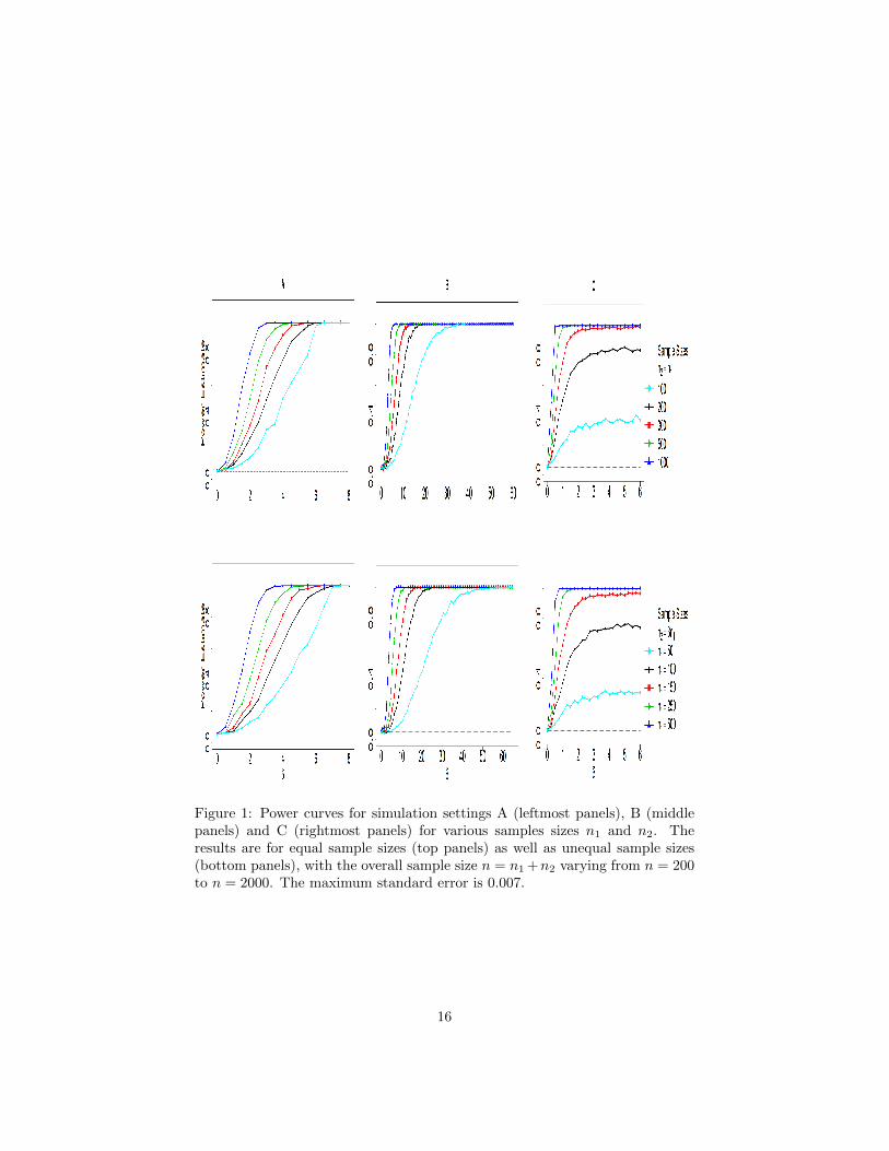
Figure 1: Power curves for simulation settings A (leftmost panels), B (middlepanels) and C (rightmost panels) for various samples sizes n1 and n2. Theresults are for equal sample sizes (top panels) as well as unequal sample sizes(bottom panels), with the overall sample size n = n1 +n2 varying from n = 200to n = 2000. The maximum standard error is 0.007.
16

(Wurtz et al., 2006) are used to generate random data from a standardized T
and standardized skewed T distribution respectively. For moderate sample sizes,385
irrespective of their equality, the probability of rejection does not converge to
1 no matter how large δ is; see the results corresponding to a total sample size
equal to n = 200 or 400. This is in agreement with our intuition that detecting
differences in higher order moments of the distribution becomes more difficult
and requires increased sample sizes. In contrast, for larger total sample sizes,390
the empirical power curve has a fast rate of increase.
4.2. Comparison with available approaches
To the authors’ best knowledge Hall & Van Keilegom (2007) is the only
available alternative method that considers hypothesis testing that the distri-
butions of two samples of curves are the same, when the observed data are noisy395
and discrete realizations of the latent curves. Their methods are presented for
dense sampling designs only; thus we restrict the comparison to this design
only. In this section we compare the performance of their proposed Cramer-von
Mises (CVM) - type test, based on the empirical distribution functions after
local-polynomial smoothing of the two samples of curves, with our FAD test.400
We generate data {(t1ij , Y1ij) : j}n1i=1 and {(t2ij , Y2ij) : j}n2
i=1 as in Hall
& Van Keilegom (2007), and for completeness we describe it below. It is as-
sumed that Y1ij = X1i(t1ij) + N(0, 0.01) and Y2ij = X2i(t2ij) + N(0, 0.09),
where X1i(t) =∑15k=1 e
−k/2Nk1iψk(t) and X2i(t) =∑15k=1 e
−k/2Nk21iψk(t) +
δ∑15k=1 k
−2Nk22iψ∗k(t), such that Nk1i, Nk21i, Nk22i ∼ iidN(0, 1). Here ψ1 ≡ 1405
and ψk(t) =√
2sin{(k− 1)πt} are orthonormal basis functions. Also ψ∗1(t) ≡ 1,
ψ∗k(t) =√
2sin{(k−1)π(2t−1)} if k > 1 is odd and ψ∗k(t) =√
2cos{(k−1)π(2t−
1)} if k > 1 is even. As before the index δ controls the deviation from the null
hypothesis; δ = 0 corresponds to the null hypothesis, that the two samples have
identical distribution. Finally, the sampling design for the curves is assumed410
balanced (m1 = m2 = m), but irregular, and furthermore different across the
two samples. Specifically, it is assumed that {t1ij : 1 ≤ i ≤ n1, 1 ≤ j ≤ m1}
are iid realizations from Uniform(0, 1), and {t2ij : 1 ≤ i ≤ n2, 1 ≤ j ≤ m2} are
17

iid realizations from the distribution with density 0.8 + 0.4t for 0 ≤ t ≤ 1. Two
scenarios are considered: i) m = 20 points per curve, and ii) m = 100 points415
per curve. The null hypothesis that the underlying distribution is identical in
the two samples is tested using CVM (Hall & Van Keilegom, 2007) and FAD
testing procedures for various values of δ. Figure 2 illustrates the comparison
between the approaches for significance level α = 0.05; the results are based on
500 Monte Carlo replications.420
The CVM test is conducted using the procedure described in Hall & Van Kei-
legom (2007), and the p-value is determined based on 250 bootstrap replicates;
the results are obtained using the R code provided by the authors. To apply
our approach, we use refund package (Crainiceanu et al., 2012) in R, which
requires that the data are formatted corresponding to a common grid of points,425
with possible missingness. Thus, a pre-processing step is necessary. For each
scenario, we consider a common grid of m equally spaced points in [0, 1] and
bin the data of each curve according to this grid. This procedure introduces
missingness for the points where no data are observed. We note that, this pre-
processing step is not necessary if one uses PACE package (Yao et al., 2005) in430
Matlab, for example. However, our preference for using open-source software,
motivates the use of refund. Comparison of refund and PACE revealed that the
two methods lead to similar results when smoothing trajectories from noisy and
sparsely observed ‘functional’ data.
As Figure 2 illustrates, both procedures maintain the desiredlevel of sig-435
nificance and the number of observations per curve m1 = m2 do not seem to
strongly impact the results. However, the empirical power of the FAD test in-
creases at a faster rate than the CVM test(Hall & Van Keilegom, 2007) under
all the settings considered. This should not seem surprising, as by representing
the data using orthogonal basis expansion as detailed in Section 3 we remove440
extraneous components. In contrast the CVM test attempts to estimate all basis
functions by smoothing the data. This can introduce error that can ultimately
lower the power of the test. Additionally, due to the usage of bootstrapping to
approximate the null distribution of the test, the CVM test has a much higher
18
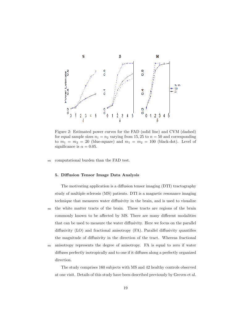
Figure 2: Estimated power curves for the FAD (solid line) and CVM (dashed)for equal sample sizes n1 = n2 varying from 15, 25 to n = 50 and correspondingto m1 = m2 = 20 (blue-square) and m1 = m2 = 100 (black-dot). Level ofsignificance is α = 0.05.
computational burden than the FAD test.445
5. Diffusion Tensor Image Data Analysis
The motivating application is a diffusion tensor imaging (DTI) tractography
study of multiple sclerosis (MS) patients. DTI is a magnetic resonance imaging
technique that measures water diffusivity in the brain, and is used to visualize
the white matter tracts of the brain. These tracts are regions of the brain450
commonly known to be affected by MS. There are many different modalities
that can be used to measure the water diffusivity. Here we focus on the parallel
diffusivity (LO) and fractional anisotropy (FA). Parallel diffusivity quantifies
the magnitude of diffusivity in the direction of the tract. Whereas fractional
anisotropy represents the degree of anisotropy. FA is equal to zero if water455
diffuses perfectly isotropically and to one if it diffuses along a perfectly organized
direction.
The study comprises 160 subjects with MS and 42 healthy controls observed
at one visit. Details of this study have been described previously by Greven et al.
19

(2011), Goldsmith et al. (2011), and Staicu et al. (2012). Parallel diffusivity and460
fractional anisotropy measurements are recorded at 93 locations along the corpus
callosum (CCA) tract - the largest brain tract that connects the two cerebral
hemispheres. Tracts are registered between subjects using standard biological
landmarks identified by an experienced neuroradiologist. For illustration, Figure
3 displays the parallel diffusivity and fractional anisotropy profiles along the465
CCA for both healthy controls and MS patients. Part of this data set is available
in the R-package refund (Crainiceanu et al., 2012).
Our objective is to study if parallel diffusivity or fractional anisotropy along
the CCA tract have the same distribution for subjects affected by MS and for
controls. Such assessment would provide researchers with valuable information470
about whether either of these modalities, along this tract, are useful in deter-
mining axonal disruption in MS. Visual inspection of the data (see Figure 3)
reveals that the average of fractional anisotropy seems to be different in cases
than controls. It appears that for fixed tract location, parallel diffusivity ex-
hibits a distribution with shape characteristics that depend on the particular475
tract location. Furthermore, the location-varying shape characteristics seem to
be different in the MS versus control groups. Staicu et al. (2012) proposed a
modeling approach that accounts for the features of the pointwise distribution
of the parallel diffusivity in the two groups. However, they did not formally in-
vestigate whether the distribution of this DTI modality is different for the two480
groups. Here we apply the proposed two-sample hypothesis testing to assess
whether the true distribution of parallel diffusivity and fractional anisotropy
respectively, along the CCA tract is the same for MS and controls.
The parallel diffusivity and fractional anisotropy profiles are typically sam-
pled on a regular grid (93 equal spaced locations); however, some subjects have485
missing data. Additionally, the observations are assumed to be contaminated
by noise. We use the methods discussed in Section 3, corresponding to sparse
sampling design. The overall mean function is estimated using penalized splines
with 10 basis functions. The functional principal component decomposition was
performed using the fpca.sc function in the R package refund and by setting490
20

Figure 3: Top: Fractional anisotropy for cases and controls with the point-wise mean in red. Bottom: Parallel diffusivity for cases and controls with thepointwise mean in red.
the percentage of explained variance parameter to τ = 95% (Crainiceanu et al.
(2012)).
5.1. Parallel Diffusivity (LO)
For the parallel diffusivity data set, Figure 4 displays the three leading eigen-
functions of the combined data, along with the box plots of the corresponding495
coefficients presented separately for the MS and control groups. The first, sec-
ond, and third functional principal component functions explain 76%, 8%, and
7% of the total variability, respectively. The first functional principal compo-
nent is negative and has a concave shape with a dip around location 60 of the
CCA tract. This component gives the direction along which the two curves differ500
the most. Near location 60 the distribution of the parallel diffusivity is highly
skewed for the MS group, but not as skew in the control group. Examination
of the boxplot of the coefficients corresponding to the first eigenfunction (left,
bottom panel of Figure 4) shows that most healthy individuals (controls) are
loaded positively on this component, yielding parallel diffusivity profiles that505
are lower than the overall average profile. Half of the MS subjects are loaded
negatively on this component resulting in increased parallel diffusivity.
The FPCA procedure estimates that five eigenfunctions account for 95% of
the total variation in the parallel diffusivity data. We apply the FAD testing
21

procedure to study whether the distributions of the five coefficients is the same510
for MS and controls. The p-values of the univariate tests are p1 = 0.00001,
p2 = 0.01206, p3 = 0.09739, p4 = 0.30480, and p5 = 0.30026; the p-value of
the FAD test is thus p = 5 × min1≤k≤5 pk = 0.00005. This shows significant
evidence that the parallel diffusivity has different distribution in MS subjects
than controls.515
Figure 4: Parallel Diffusivity (LO). Top: First three eigenfunctions of the com-bined data set. Bottom: Box plots of the first three group specific combinedscores. The eigenfunctions explain 91% of the total variation.
5.2. Fractional Anisotropy (FA)
We turn next to the analysis of the fractional anisotropy in controls and MS
cases. Figure 5 illustrates the leading four eigenfunctions of the combined sample
(which explain about 90% of the entire variability), along with the boxplots of520
the distributions of the corresponding controls/cases coefficients. The estimated
first eigenfunction implies that the two samples differ in the mean function.
Six functional principal components are selected to explain 95% of the total
variation. Using the p-values of the six univariate tests are p1 ≈ 0, p2 = 0.29539,
22

p3 = 0.00804, p4 = 0.56367, p5 = 0.51001, and p6 = 0.21336; the p-value of the525
FAD test is thus p = 6×min1≤k≤6 pk ≈ 0. This shows significant evidence that
the FA has different distribution in MS subjects than controls.
Figure 5: Fractional Anisotropy. Top: First four eigenfunctions of the combinedFA data set. Bottom: Box plots of the four three group specific combined scores.The eigenfunctions explain 90% of the total variation.
6. Discussion
When dealing with functional data, which is infinite dimensional, it is im-
portant to use data reduction techniques that take advantage of the functional530
nature of the data. In particular FPCA allows to represent a set of curves using
typically a low dimensional space. By using FPCA to represent the two samples
of curves, we are able to reduce the dimension of the testing problem and apply
well known lower-dimensional procedures.
In this paper, we propose a novel testing method capable of detecting differ-535
ences between the generating distribution of two groups of curves. The proposed
approach is based on classical univariate procedures (e.g. Anderson-Darling
test), scales well to larger samples sizes, and can be easily extended to test
the null hypothesis that multiple (as in more than two) groups of curves have
identical distribution. We found that the KS test has similar attributes but was540
23

not as powerful for detecting changes in the higher order moments of the coef-
ficient distributions. Furthermore, we have shown that the proposed FAD test
outperforms the CVM test of Hall & Van Keilegom (2007) for smaller sample
sizes.
7. Acknowledgments545
We thank Daniel Reich and Peter Calabresi for the DTI tractography data.
Pomann’s research is supported by the National Science Foundation under Grant
No. DGE-0946818. Ghosh’s research was supported in part by the NSF under
grant DMS-1358556. The authors are grateful to Ingrid Van Keilegom for shar-
ing the R code used in Hall & Van Keilegom (2007).550
APPENDIX
References
Aslan, B., & Zech, G. (2005). New test for the multivariate two-sample problem
based on the concept of minimum energy. Journal of Statistical Computation
and Simulation, 75 , 109–119.555
Aston, J. A., Chiou, J.-M., & Evans, J. P. (2010). Linguistic pitch analysis
using functional principal component mixed effect models. Journal of the
Royal Statistical Society: Series C (Applied Statistics), 59 , 297–317.
Benko, M., Hardle, W., & Kneip, A. (2009). Common functional principal
components. The Annals of Statistics, 37 .560
Besse, P., & Ramsay, J. (1986). Principal components analysis of sampled
functions. Psychometrika, 51 , 285–311.
Bohm, G., & Zech, G. (2010). Introduction to statistics and data analysis for
physicists. DESY.
Bosq, D. (2000). Linear processes in function spaces: theory and applications565
volume 149. Springer.
24

Chiou, J.-M., Muller, H.-G., Wang, J.-L., & Carey, J. R. (2003). A functional
multiplicative effects model for longitudinal data, with application to repro-
ductive histories of female medflies. Statistica Sinica, 13 , 1119.
Crainiceanu, C., Reiss, P., Goldsmith, J., Huang, L., Huo, L., Scheipl, F.,570
Greven, S., Harezlak, J., Kundu, M. G., & Zhao, Y. (2012). refund :
Regression with functional data. R Package 0.1-6 , . URL: http://cran.
r-project.org/web/packages/refund/refund.pdf.
Cuevas, A., Febrero, M., & Fraiman, R. (2004). An anova test for functional
data. Computational statistics & data analysis, 47 , 111–122.575
Di, C., Crainiceanu, C. M., Caffo, B. S., & Naresh M. Punjabi, N. M. (2009).
Multilevel functional principal component analysis. The annals of Applied
Statistics, 3 , 458–488.
Estevez-Perez, G., & Vilar, J. A. (2008). Functional anova starting from dis-
crete data: an application to air quality data. Environmental and Ecological580
Statistics, 20 , 495–515.
Ferraty, F., Vieu, P., & Viguier-Pla, S. (2007). Factor-based comparison of
groups of curves. Computational Statistics & Data Analysis, 51 , 4903–4910.
Fremdt, S., Horvath, L., Kokoszka, P., & Steinebach, J. (2012). Testing the
equality of covariance operators in functional samples. Scand. J. Statist., 40 ,585
138–152.
Friedman, J., & Rafsky, L. (1979). Multivariate generalizations of the wald-
wolfowitz and smirnov two-sample tests. The Annals of Statistics, 7 , 697–
717.
Goldsmith, J., Bobb, J., Crainiceanu, C., Caffo, B., & Reich, D. (2011). Penal-590
ized functional regression. Journal of Computational and Graphical Statistics,
20 , 850–851.
25

Greven, S., Crainiceanu, C., Caffo, B., & Reich, D. (2011). Longitudinal func-
tional principal component analysis. In Recent Advances in Functional Data
Analysis and Related Topics (pp. 149–154). Springer.595
Hall, P., Muller, H.-G., & Wang, J.-L. (2006). Properties of principal component
methods for functional and longitudinal data analysis. Annals of Statistics,
34 , 1493–1517.
Hall, P., & Van Keilegom, I. (2007). Two-sample tests in functional data analysis
starting from discrete data. Statistica Sinica, 17 , 1511.600
Horvath, L., & Kokoszka, P. (2012). Inference for functional data with applica-
tions volume 200. Springer.
Horvath, L., Kokoszka, P., & Reeder, R. (2013). Estimation of the mean of func-
tional time series and a two-sample problem. Journal of the Royal Statistical
Society: Series B (Statistical Methodology), 75 , 103–122.605
Kraus, D., & Panaretos, V. (2012). Dispersion operators and resistant second-
order analysis of functional data. Biometrika, 99 .
Laukaitis, A., & Rackauskas, A. (2005). Functional data analysis for clients
segmentation tasks. European journal of operational research, 163 , 210–216.
Massey Jr, F. (1951). The kolmogorov-smirnov test for goodness of fit. Journal610
of the American statistical Association, 46 , 68–78.
Pettitt, A. N. (1976). A two-sample anderson-darling rank statistic. Biometrika,
63 , 161–168.
Ramsay, J., & Silverman, B. (2005). Functional Data Analysis. Springer.
Read, T., & Cressie, N. (1988). Goodness-of-fit statistics for discrete multivari-615
ate data volume 7. Springer-Verlag New York.
Rice, J. A., & Silverman, B. W. (1991). Estimating the mean and covariance
structure nonparametrically when the data are curves. Journal of the Royal
Statistical Society. Series B (Methodological), 53 , 233–243.
26
Schilling, M. (1986). Multivariate two-sample tests based on nearest neighbors.620
Journal of the American Statistical Association, 81 , 799–806.
Scholz, F. (2011). R package adk.
Scholz, F., & Stephens, M. (1987). K-sample anderson–darling tests. Journal
of the American Statistical Association, 82 , 918–924.
Staicu, A.-M., Crainiceanu, C. M., & Carroll, R. J. (2010). Fast methods for625
spatially correlated multilevel functional data. Biostatistics, 11 , 177–194.
Staicu, A.-M., Crainiceanu, C. M., Reich, D. S., & Ruppert, D. (2012). Modeling
functional data with spatially heterogeneous shape characteristics. Biomet-
rics, 68 , 331–343. URL: http://dx.doi.org/10.1111/j.1541-0420.2011.
01669.x. doi:10.1111/j.1541-0420.2011.01669.x.630
Staicu, A.-M., Li, Y., Crainiceanu, C. M., & Ruppert, D. (2014). Likelihood
ratio tests for dependent data with applications to longitudinal and functional
data analysis. Scandinavian Journal of Statistics, to appear . URL: http:
//www4.stat.ncsu.edu/~staicu/papers/pLRT_final_version.pdf.
Staniswalis, J. G., & Lee, J. J. (1998). Nonparametric regression analysis of635
longitudinal data. Journal of the American Statistical Association, 93 , 1403–
1418.
Stephens, M. A. (1974). Edf statistics for goodness of fit and some comparisons.
Journal of the American Statistical Association, 69 , pp. 730–737. URL: http:
//www.jstor.org/stable/2286009.640
Wei, L., & Lachin, J. (1984). Two-sample asymptotically distribution-free tests
for incomplete multivariate observations. Journal of the American Statistical
Association, 79 , 653–661.
Wurtz, D., Chalabi, Y., & Luksan, L. (2006). Parameter estimation of arma
models with garch/aparch errors an r and splus software implementation.645
27

Yao, F., Muller, H., & Wang, J. (2005). Functional data analysis for sparse
longitudinal data. JASA, 100 , 577–591.
Zhang, J.-T., & Chen, J. (2007). Statistical inferences for functional data. The
Annals of Statistics, 35 , 1052–1079.
Zhang, J.-T., Liang, X., & Xiao, S. (2010). On the two-sample behrens-fisher650
problem for functional data. Journal of Statistical Theory and Practice, 4 ,
571–587.
28


