

Uncertainty Quantification in Ill-Posed Inverse Problems:Case Studies in the Physical Sciences
Mikael KuuselaDepartment of Statistics and Data Science
Carnegie Mellon University
CERN-EP/IT Data Science Seminar
April 1, 2020
Mikael Kuusela (CMU) April 1, 2020 1 / 40

Motivation: Heat equation
Consider the heat equation on the real line:{∂u(x ,t)∂t = k ∂
2u(x ,t)∂x2 , (x , t) ∈ R× [0,∞),
u(x , 0) = f (x), x ∈ R
Forward problem: Given the initial condition f (x) = u(x , 0), what is thetemperature distribution g(x) = u(x , t∗) at time t∗?
Inverse problem: Given the temperature distribution g(x) = u(x , t∗) attime t∗, what was the initial distribution f (x) = u(x , 0) at time t = 0?
Mikael Kuusela (CMU) April 1, 2020 2 / 40

Motivation: Heat equation
The forward problem is easy:
u(x , t) =
∫ ∞−∞
Φt(x − y)f (y) dy
where
Φt(x) =1√
4πktexp
(− x2
4kt
)
So we have a well-defined integral operator K that maps the initialdistribution f to the distribution g at time t∗:
g(x) = u(x , t∗) =
∫ ∞−∞
Φt∗(x − y)f (y) dy = (Kf )(x)
The inverse problem is to solve g = Kf for f . This is fundamentallydifficult. Let’s see why.
Mikael Kuusela (CMU) April 1, 2020 3 / 40

Motivation: Heat equation
-25 -20 -15 -10 -5 0 5 10 15
0
0.01
0.02
0.03
0.04
0.05
0.06
0.07
0.08
0.09
0.1Initial distribution
Distribution at time t=0.05
Temperature distribution at time t = 0.05
Mikael Kuusela (CMU) April 1, 2020 4 / 40

Motivation: Heat equation
-25 -20 -15 -10 -5 0 5 10 15
0
0.01
0.02
0.03
0.04
0.05
0.06
0.07
0.08
0.09
0.1Initial distribution
Distribution at time t=0.2
Temperature distribution at time t = 0.2
Mikael Kuusela (CMU) April 1, 2020 4 / 40

Motivation: Heat equation
-25 -20 -15 -10 -5 0 5 10 15
0
0.01
0.02
0.03
0.04
0.05
0.06
0.07
0.08
0.09
0.1Initial distribution
Distribution at time t=0.5
Temperature distribution at time t = 0.5
Mikael Kuusela (CMU) April 1, 2020 4 / 40

Motivation: Heat equation
-25 -20 -15 -10 -5 0 5 10 15
0
0.01
0.02
0.03
0.04
0.05
0.06
0.07
0.08
0.09
0.1Initial distribution
Distribution at time t=1
Temperature distribution at time t = 1
Mikael Kuusela (CMU) April 1, 2020 4 / 40

Motivation: Heat equation
-25 -20 -15 -10 -5 0 5 10 15
0
0.01
0.02
0.03
0.04
0.05
0.06
0.07
0.08
0.09
0.1Initial distribution
Distribution at time t=10
Temperature distribution at time t = 10
Mikael Kuusela (CMU) April 1, 2020 4 / 40

Motivation: Heat equation
-25 -20 -15 -10 -5 0 5 10 15
0
0.01
0.02
0.03
0.04
0.05
0.06
0.07
0.08
0.09
0.1Initial distribution
Distribution at time t=100
Temperature distribution at time t = 100
Mikael Kuusela (CMU) April 1, 2020 4 / 40

Motivation: Heat equation
Now, consider the two initial distributions shown below and run themforward in time.
-25 -20 -15 -10 -5 0 5 10 15
0
0.01
0.02
0.03
0.04
0.05
0.06
0.07
0.08
0.09
0.1Initial distribution
-25 -20 -15 -10 -5 0 5 10 15
0
0.01
0.02
0.03
0.04
0.05
0.06
0.07
0.08
0.09
0.1Initial distribution
Mikael Kuusela (CMU) April 1, 2020 5 / 40

Motivation: Heat equation
Now, consider the two initial distributions shown below and run themforward in time.
-25 -20 -15 -10 -5 0 5 10 15
0
0.01
0.02
0.03
0.04
0.05
0.06
0.07
0.08
0.09
0.1Initial distribution
Distribution at time t=1
-25 -20 -15 -10 -5 0 5 10 15
0
0.01
0.02
0.03
0.04
0.05
0.06
0.07
0.08
0.09
0.1Initial distribution
Distribution at time t=1
The distributions at time t = 1 are almost indistinguishable!
If the distribution at time t = 1 is observed with even the tiniest amountof noise, then there is no way to distinguish between these two initialdistributions based on the distribution at time t = 1
Mikael Kuusela (CMU) April 1, 2020 5 / 40

Ill-posed inverse problems
Ill-posed inverse problems are problems of the type
g = K (f ),
where the mapping K is such that it can take inputs f1 and f2 that lookvery different into outputs g1 and g2 that are very similar
This means that, without further information, data collected in theg -space can only mildly constrain the solution in the f -space
Mikael Kuusela (CMU) April 1, 2020 6 / 40
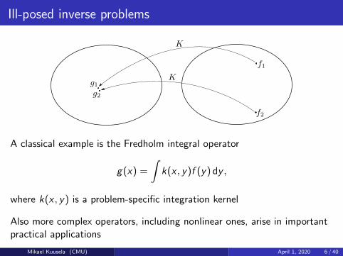
Ill-posed inverse problems
A classical example is the Fredholm integral operator
g(x) =
∫k(x , y)f (y) dy ,
where k(x , y) is a problem-specific integration kernel
Also more complex operators, including nonlinear ones, arise in importantpractical applications
Mikael Kuusela (CMU) April 1, 2020 6 / 40
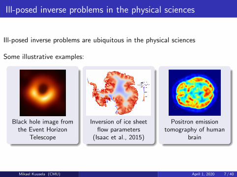
Ill-posed inverse problems in the physical sciences
Ill-posed inverse problems are ubiquitous in the physical sciences
Some illustrative examples:
Black hole image fromthe Event Horizon
Telescope
Inversion of ice sheetflow parameters
(Isaac et al., 2015)
Positron emissiontomography of human
brain
Mikael Kuusela (CMU) April 1, 2020 7 / 40

Case studies
Throughout this talk, I will specifically focus on the following two problems:
Large Hadron Collider
Unfolding of detector smearing indifferential cross-section measurements
Orbiting Carbon Observatory-2
Space-based retrieval of atmosphericcarbon dioxide concentration
Mikael Kuusela (CMU) April 1, 2020 8 / 40

The unfolding problem
Any differential cross section measurement is affected by the finiteresolution of the particle detectors
This causes the observed spectrum of events to be “smeared” or“blurred” with respect to the true one
The unfolding problem is to estimate the true spectrum using thesmeared observations
Ill-posed inverse problem with major methodological challenges
−5 0 50
500
1000
1500
Physical observable
(b) Smeared intensity
Intensity
Figure: Smeared spectrum
Folding←−−Unfolding−−→
−5 0 50
500
1000
1500
Physical observable
(a) True intensity
Intensity
Figure: True spectrum
Mikael Kuusela (CMU) April 1, 2020 9 / 40

Problem formulation
Let f be the true, particle-level spectrum and g the smeared, detector-levelspectrum
Denote the true space by T and the smeared space by S (both takento be intervals on the real line for simplicity)Mathematically f and g are the intensity functions of the underlyingPoisson point process
The two spectra are related by
g(s) =
∫T
k(s, t)f (t) dt,
where the smearing kernel k represents the response of the detector and isgiven by
k(s, t) = p(Y = s|X = t,X observed)P(X observed|X = t),
where X is a true event and Y the corresponding smeared event
Task: Infer the true spectrum f given smeared observations from g
Mikael Kuusela (CMU) April 1, 2020 10 / 40
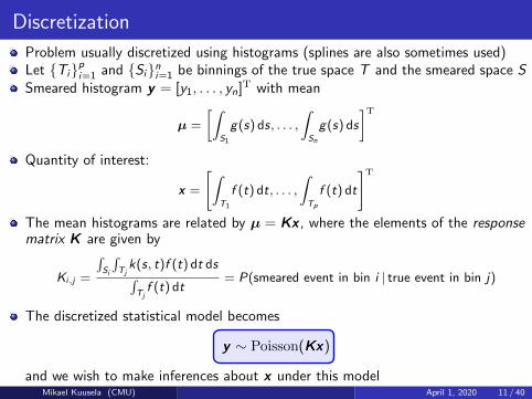
Discretization
Problem usually discretized using histograms (splines are also sometimes used)Let {Ti}pi=1 and {Si}ni=1 be binnings of the true space T and the smeared space SSmeared histogram y = [y1, . . . , yn]T with mean
µ =
[∫S1
g(s) ds, . . . ,
∫Sn
g(s) ds
]TQuantity of interest:
x =
[∫T1
f (t) dt, . . . ,
∫Tp
f (t) dt
]TThe mean histograms are related by µ = Kx , where the elements of the responsematrix K are given by
Ki,j =
∫Si
∫Tjk(s, t)f (t) dt ds∫Tjf (t) dt
= P(smeared event in bin i | true event in bin j)
The discretized statistical model becomes
y ∼ Poisson(Kx)
and we wish to make inferences about x under this modelMikael Kuusela (CMU) April 1, 2020 11 / 40

OCO-2: general model
x ∈ Rp: state vector, F ∈ Rp → Rn: forward model,ε ∈ Rn: instrument noise, y ∈ Rn: radiance observations
Mikael Kuusela (CMU) April 1, 2020 12 / 40

OCO-2: linearized surrogate model (Hobbs et al., 2017)
State vector x :
CO2 profile (layer 1 to layer 20) [20 elements]surface pressure [1 elements]surface albedo [6 elements]aerosols [12 elements]
Forward model F : linearized using the Jacobian K (x) = ∂F (x)∂x
Noise ε: normal approximation of Poisson noise
Observations y : radiances in 3 near-infrared bands [1024 in each band]
O2 A-band (around 0.76 microns)weak CO2 band (around 1.61 microns)strong CO2 band (around 2.06 microns)
Mikael Kuusela (CMU) April 1, 2020 13 / 40

Synthesis
Both HEP unfolding and CO2 remote sensing can be approximatedreasonably well using the Gaussian linear model:
y = Kx + ε, ε ∼ N(0,Σ),
where y ∈ Rn are the observations, x ∈ Rp is the unknown quantity andK ∈ Rn×p is an ill-conditioned matrix
A few caveats:
May have n ≥ p or n < p
Even when n ≥ p, may have rank(K ) < p
Usually have physical constraints for x , for example x ≥ 0
The fundamental problem, though, is that K has a huge condition number
Mikael Kuusela (CMU) April 1, 2020 14 / 40

Regularization
In both fields, the standard approaches1 for handling the ill-posedness arevery similar
Find a regularized solution by solving
x = minx∈Rp
(y −Kx)TΣ−1(y −Kx) + δ‖L(x − xa)‖2 (∗)
Here, the first term is a data-fit term and the second term penalizesphysically implausible solutions
→ Balances the competing requirements of fitting the data and finding awell-behaved solution (bias-variance trade-off)
Two viewpoints — the same answer:1 Frequentist: Penalized maximum likelihood
x = maxx∈Rp
log L(x)− δP(x)⇒ (∗)
2 Bayesian: Using prior x ∼ N(xa, 1δ (LTL)−1), estimate x using the
mean/maximum of the posterior p(x |y) ∝ p(y |x)p(x)⇒ (∗)1There are many variants of these ideas, but the fundamental issues remain the same.
Mikael Kuusela (CMU) April 1, 2020 15 / 40

Regularized uncertainty quantification
For the rest of this talk, let’s assume that we are interested in some functional (orpotentially some collection of functionals) of x
Let θ = hTx be a quantity of interest; for example
OCO-2: θ = XCO2 = weighted average of the CO2 profile
HEP: θ = eTi x = ith unfolded bin or θ = aggregate of several unfolded bins
In both frequentist and Bayesian approaches, a natural estimator of θ is θ = hTx
While the frequentist and Bayesian perspectives lead to the same pointestimators θ, the associated uncertainties are different:
1 Frequentist: 1− α variability intervals
[θ, θ] = [θ − z1−α/2
√var(θ), θ + z1−α/2
√var(θ)]
2 Bayesian: 1− α posterior credible intervals
[θ, θ] = [θ − z1−α/2
√var(θ|y), θ + z1−α/2
√var(θ|y)]
HEP unfolding typically takes approach 1 , while remote sensing uses 2
Mikael Kuusela (CMU) April 1, 2020 16 / 40

Regularization and frequentist coverage
Let’s assume that ultimately we would like to quantify the uncertainty of θusing a confidence interval with well-calibrated frequentist coverage
That is, for a given confidence level 1− α, we are looking for a randominterval [θ, θ] such that
P (θ ∈[θ, θ]) ≈ 1− α, for any x
When constructed based on a regularized point estimator x , both thefrequentist variability interval and the Bayesian credible interval havetrouble satisfying this criterion
There are always x ’s such that the regularized estimator x is biased (i.e.,E(x) 6= x) and the estimator θ inherits this bias
Variability intervals ignore the bias and only account for the variance⇒ Undercoverage when large bias, correct coverage when small bias
Credible intervals are always wider than the variability intervals⇒ Undercoverage when large bias, overcoverage when small bias
Mikael Kuusela (CMU) April 1, 2020 17 / 40

Regularization and frequentist coverage
When the noise is Gaussian with known covariance, it is possible to writedown the coverage of these intervals in closed form:
1 Variability intervals
P (θ ∈ [θ, θ]) = Φ
bias(θ)√var(θ)
+ z1−α/2
− Φ
bias(θ)√var(θ)
− z1−α/2
2 Credible intervals
P (θ ∈ [θ, θ]) = Φ
bias(θ)√var(θ)
+ z1−α/2
√var(θ|y)
var(θ)
− Φ
bias(θ)√var(θ)
− z1−α/2
√var(θ|y)
var(θ)
Both of these are even functions of bias(θ) and maximized when bias(θ) = 0
The variability intervals have coverage 1− α if and only if bias(θ) = 0;otherwise coverage < 1− αThe credible intervals have coverage > 1− α for bias(θ) = 0; coverage 1− αfor a certain value of |bias(θ)|; and coverage < 1− α for large |bias(θ)|
Mikael Kuusela (CMU) April 1, 2020 18 / 40

Unfolding: Simulation setup
-5 0 5
0
200
400
600
800
1000
1200
Inte
nsity
True
Smeared f (t) = λtot
{π1N (t|−2, 1) + π2N (t|2, 1) + π3
1
|T |
}g(s) =
∫TN (s − t|0, 1)f (t) dt
f MC(t) = λtot
{π1N (t|−2, 1.12) + π2N (t|2, 0.92) + π3
1
|T |
}
Mikael Kuusela (CMU) April 1, 2020 19 / 40

Undercoverage in unfolding
10 -1 10 0 10 1 10 2 10 3 10 4 10 5
0
0.2
0.4
0.6
0.8
1
C
ove
rag
e a
t rig
ht
pe
ak
(a) SVD variant of Tikhonov regularization
−5 0 50
0.2
0.4
0.6
0.8
1(a) SVD, weighted CV
Bin
wis
e c
ove
rage
Coverage in SVD unfolding: as a function of the regularization strength (left)and for cross-validated regularization strength (right)
Mikael Kuusela (CMU) April 1, 2020 20 / 40

Bias and coverage for operational OCO-2 retrievals
(a) Bias distribution (b) Coverage distribution
Bias (left) and coverage (right) for operational OCO-2 retrievals forseveral realizations of the state vector x
Mikael Kuusela (CMU) April 1, 2020 21 / 40
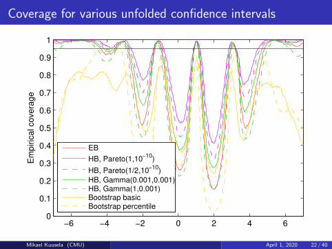
Coverage for various unfolded confidence intervals
−6 −4 −2 0 2 4 60
0.1
0.2
0.3
0.4
0.5
0.6
0.7
0.8
0.9
1E
mp
iric
al co
ve
rag
e
EB
HB, Pareto(1,10−10
)
HB, Pareto(1/2,10−10
)
HB, Gamma(0.001,0.001)HB, Gamma(1,0.001)Bootstrap basicBootstrap percentile
Mikael Kuusela (CMU) April 1, 2020 22 / 40

Unregularized inversion?
At the end of the day, any regularization technique makes unverifiableassumptions about the true solution
If these assumptions are not satisfied, the uncertainties will be wrongIn the absence of oracle information about the true x , there does not seemto be any obvious way around this
So maybe we should reconsider whether explicit regularization is such a goodidea to start with?Instead of finding a regularized estimator of x , what if we simply used theunregularized maximum likelihood / least squares estimator
x = minx∈Rp
(y −Kx)TΣ−1(y −Kx)
When K has full column rank, the solution is x = (KTΣ−1K )−1KTΣ−1yThis is unbiased (E(x) = x) and hence also the corresponding estimatorθ = hTx of the functional θ = hTx is unbiasedTherefore, by the previous discussion, the variability interval
[θ, θ] = [θ − z1−α/2
√var(θ), θ + z1−α/2
√var(θ)]
has correct coverage 1− αMikael Kuusela (CMU) April 1, 2020 23 / 40

Implicit regularization
Of course, when K is ill-conditioned, the unregularized estimator x willhave a huge variance
But this does not mean that θ = hTx needs to have a huge variance!
The mapping x 7→ θ = hTx can act as an implicit regularizer resulting ina well-constrained interval [θ, θ] for the functional θ = hTxThis is especially the case when the functional is a smoothing oraveraging operation, for example:
Inference for wide unfolded bins (demo to follow)XCO2 in OCO-2 (average CO2 over the atmospheric column)
Of course, there are also functionals that are more difficult to constrain(e.g, point evaluators θ = eT
i x , derivatives,...)
In those cases, the intervals [θ, θ] are wide—as they should be, sincethere is simply not enough information in the data y to constrain thesefunctionals
Mikael Kuusela (CMU) April 1, 2020 24 / 40

Wide bin unfolding
In the case of unfolding, one functional we should be able to recoverwithout explicit regularization is the integral of f over a wide unfoldedbin:
Hj [f ] =
∫Tj
f (t) dt, width of Tj large
But one cannot simply arbitrarily increase the particle-level bin size in theconventional approaches, since this increases the MC dependence of KTo circumvent this, it is possible to first unfold with fine bins (and noregularization) and then aggregate into wide bins
Let’s see how this works using a similar deconvolution setup as before
Mikael Kuusela (CMU) April 1, 2020 25 / 40

Wide bins, standard approach, perturbed MC
-6 -4 -2 0 2 4 60
500
1000
1500
2000
2500
Inte
nsity
Unfolded
True
-6 -4 -2 0 2 4 60
0.1
0.2
0.3
0.4
0.5
0.6
0.7
0.8
Bin
wis
e c
ove
rag
e
The response matrix Ki ,j =
∫Si
∫Tjk(s,t)f MC(t) dt ds∫Tjf MC(t) dt
depends on f MC
⇒ Undercoverage if f MC 6= f
Mikael Kuusela (CMU) April 1, 2020 26 / 40

Wide bins, standard approach, correct MC
-6 -4 -2 0 2 4 60
500
1000
1500
2000
2500
Inte
nsity
Unfolded
True
-6 -4 -2 0 2 4 60
0.1
0.2
0.3
0.4
0.5
0.6
0.7
0.8
Bin
wis
e c
ove
rag
e
If f MC = f , coverage is correct
⇒ But this situation is unrealistic because f of course is unknown
Mikael Kuusela (CMU) April 1, 2020 27 / 40

Fine bins, standard approach, perturbed MC
-6 -4 -2 0 2 4 6
-4000
-2000
0
2000
4000
6000
8000
Inte
nsity
Unfolded
True
-6 -4 -2 0 2 4 60
0.1
0.2
0.3
0.4
0.5
0.6
0.7
0.8
Bin
wis
e c
ove
rag
e
With narrow bins, less dependence on f MC so coverage is correct, but theintervals are very wide2
⇒ Let’s aggregate these into wide bins, keeping track of the bin-to-bincorrelations in the error propagation
2More unfolded realizations given in the backup .Mikael Kuusela (CMU) April 1, 2020 28 / 40
Wide bins via fine bins, perturbed MC
-6 -4 -2 0 2 4 60
500
1000
1500
2000
2500
Inte
nsity
Unfolded
True
-6 -4 -2 0 2 4 60
0.1
0.2
0.3
0.4
0.5
0.6
0.7
0.8
Bin
wis
e c
ove
rag
e
Wide bins via fine bins gives both correct coverage and intervals withreasonable length3
3More unfolded realizations given in the backup .Mikael Kuusela (CMU) April 1, 2020 29 / 40

Relaxing the full rank assumption
This simple approach works as long as the forward model K has fullcolumn rank and there are no constraints that x needs to satisfy
The full rank requirement can be quite restrictive in practice, for example:
Unfolding with more true bins p than smeared bins n ⇒ Kcolumn-rank deficient
The linearized OCO-2 forward model has n� p, but is neverthelesscolumn-rank deficient
When K is column-rank deficient, it has a non-trivial null space ker(K )
Therefore, confidence intervals for θ = hTx would need to be infinitelylong if there are no constraints on x (assuming h not orthogonal to ker(K ))
However, simple constraints such as x ≥ 0 or Ax ≤ b can be enough tomake the intervals finite
And we would in any case like to make use of constraints, if available
Mikael Kuusela (CMU) April 1, 2020 30 / 40

Strict bounds: Motivation
So the question becomes:
Assuming model y = Kx + ε, where K need not have full columnrank, how does one obtain a finite-sample 1 − α confidence intervalfor the linear functional θ = hTx subject to the constraint Ax ≤ b?
In the following:
We assume that we have transformed the problem so that ε ∼ N(0, I )
We denote the noise-free data by µ = Kx
Mikael Kuusela (CMU) April 1, 2020 31 / 40

Strict bounds (e.g., Stark (1992))
Rn
y space
Rp
x space
yΞ
D = K−1(Ξ)C
x
K
µ
R
hT
θ θθ
θ = hTx , θ = minx∈C∩D
hTx , θ = maxx∈C∩D
hTx
P(µ ∈ Ξ) ≥ 1− α ⇒ P(x ∈ D) ≥ 1− α⇒ P(x ∈ C ∩ D) ≥ 1− α⇒ P(θ ∈ [θ, θ]) ≥ 1− α
Mikael Kuusela (CMU) April 1, 2020 32 / 40

Strict bounds
If we construct the confidence set Ξ as
Ξ = {µ ∈ Rn : ‖y − µ‖2 ≤ χ2n,1−α},
then the endpoints of the confidence interval for θ are given by thesolutions of the following two quadratic programs:
minimize hTxsubject to ‖y −Kx‖2 ≤ χ2
n,1−αAx ≤ b
andmaximize hTxsubject to ‖y −Kx‖2 ≤ χ2
n,1−αAx ≤ b
The resulting interval [θ, θ] has by construction coverage at least 1− α
Mikael Kuusela (CMU) April 1, 2020 33 / 40

Strict bounds
The main limitation of the previous construction is that there is slack inthe last step:
P(x ∈ C ∩ D) ≥ 1− α ⇒ P(θ ∈ [θ, θ]) ≥ 1− α
Because C ∩ D is a simultaneous confidence set for x , this constructionyields simultaneous confidence intervals for any arbitrarily large collectionof functionals of x
This means that, if evaluated as a one-at-a-time interval, [θ, θ] from thisconstruction is necessarily conservative (i.e., it has overcoverage)
Mikael Kuusela (CMU) April 1, 2020 34 / 40

One-at-a-time strict bounds
Denote s2 = minAx≤b ‖y −Kx‖2.
It has been conjectured (Rust and Burrus, 1972) that the followingmodification gives a better one-at-a-time interval:
minimize hTxsubject to ‖y −Kx‖2 ≤ z2
1−α/2 + s2
Ax ≤ b
andmaximize hTxsubject to ‖y −Kx‖2 ≤ z2
1−α/2 + s2
Ax ≤ b
The coverage of these intervals has been “proven” (Rust and O’Leary,1994) and then “disproven” (Tenorio et al., 2007) so, as of now, there islimited theoretical understanding of their properties
We hope to ultimately prove the coverage, but for now we’ll simply goahead and empirically see how these perform in the CO2 retrieval problemwith the constraint x1, . . . , x21 ≥ 0 and column-rank deficient K
Mikael Kuusela (CMU) April 1, 2020 35 / 40

Coverage for OCO-2 retrievals
Mikael Kuusela (CMU) April 1, 2020 36 / 40

Coverage for OCO-2 retrievals
Table: Comparison of 95% Bayesian credible intervals (operational) and theone-at-a-time strict bounds intervals (proposed) for inference of XCO2 in OCO-2.
x operational operational operational proposed proposed proposedrealization bias coverage length coverage avg. length length s.d.
1 1.4173 0.7899 3.94 0.9515 11.20 0.292 1.3707 0.8090 3.94 0.9511 11.20 0.283 1.2986 0.8363 3.94 0.9510 11.20 0.294 1.2357 0.8579 3.94 0.9515 11.20 0.285 1.1590 0.8816 3.94 0.9513 11.20 0.286 1.0747 0.9042 3.94 0.9512 11.21 0.277 0.9721 0.9272 3.94 0.9515 11.20 0.298 0.8420 0.9500 3.94 0.9513 11.19 0.319 0.6477 0.9730 3.94 0.9508 11.19 0.3210 0.0001 0.9959 3.94 0.9502 11.18 0.35
Mikael Kuusela (CMU) April 1, 2020 37 / 40

One-at-a-time strict bounds: Discussion
We have tried more complex constraints of the form Ax ≤ b and so farthe one-at-a-time strict bounds have always had coverage at least 1− αThe intervals have excellent empirical coverage but, as of now, we aremissing a rigorous proof of coverage and/or optimality
The price to pay for good calibration is an increased interval length incomparison to regularization-based intervals
The OCO-2 problem has n� p and rank(K ) = p − 1
Do these intervals still work when p > n or rank(K )� p?
There are a few things we can say about these intervals though:
They are variable length (as opposed to fixed length in traditionalconstructions); important since there are known optimality results for fixedlength intervals (Donoho, 1994)In the case of full column rank K and no constraints on x , they reduce tothe classical fixed-length variability interval
Mikael Kuusela (CMU) April 1, 2020 38 / 40

Conclusions
Regularization works well for point estimation, but uncertaintyquantification based on regularized estimators is very difficult
Intervals from both frequentist and Bayesian constructions tend to havepoor frequentist calibration
It seems that there is a need for a major rethinking of the role ofregularization
Any explicit regularization really means some amount of “cheating” in theuncertaintiesWe should probably avoid explicit regularization and instead provideuncertainties for functionals that implicitly regularize the problemA simple example is to first unfold with narrow bins and then aggregateinto wide bins
One-at-a-time strict bounds provide good calibration even in situationswhere classical intervals do not applyAcknowledgments:
HEP unfolding: Joint work with Victor Panaretos, Philip Stark and LyleKim, with valuable input from members of the CMS Statistics CommitteeCO2 retrieval: Joint work with Pratik Patil and Jonathan Hobbs, withvaluable input from scientists at NASA Jet Propulsion Laboratory
Mikael Kuusela (CMU) April 1, 2020 39 / 40

STAMPS @ CMU
The Statistical Methods for the Physical Sciences (STAMPS) Focus Group atCMU develops statistical methods for analyzing large and complex datasets arisingacross the physical sciences.
Coordinated by: Ann Lee and Mikael Kuusela
Application areas include:
Common statistical themes: spatio-temporal data, ill-posed inverse problems,uncertainty quantification, high-dimensional data, non-Gaussian data, large-scalesimulations, massive datasets,...
See: http://stat.cmu.edu/stamps/
Mikael Kuusela (CMU) April 1, 2020 40 / 40

References I
T. Adye. Unfolding algorithms and tests using RooUnfold. In H. B. Prosper andL. Lyons, editors, Proceedings of the PHYSTAT 2011 Workshop on Statistical IssuesRelated to Discovery Claims in Search Experiments and Unfolding, CERN-2011-006,pages 313–318, CERN, Geneva, Switzerland, 17–20 January 2011.
V. Blobel. Unfolding methods in high-energy physics experiments. In CERN YellowReport 85-09, pages 88–127, 1985.
V. Blobel, The run manual: Regularized unfolding for high-energy physics experiments,OPAL Technical Note TN361, 1996.
J. Bourbeau and Z. Hampel-Arias, PyUnfold: A Python package for iterative unfolding,The Journal of Open Source Software, 3(26):741, 2018.
A. Bozson, G. Cowan, and F. Spano, Unfolding with Gaussian processes, 2018.
G. Choudalakis. Fully Bayesian unfolding. arXiv:1201.4612v4 [physics.data-an], 2012.
G. D’Agostini, A multidimensional unfolding method based on Bayes’ theorem, NuclearInstruments and Methods A, 362:487–498, 1995.
A. P. Dempster, N. M. Laird, and D. B. Rubin, Maximum likelihood from incompletedata via the EM algorithm, Journal of the Royal Statistical Society. Series B(Methodological), 39(1):1–38, 1977.
Mikael Kuusela (CMU) April 1, 2020 41 / 40

References II
D. L. Donoho, Statistical estimation and optimal recovery, The Annals of Statistics, 22(1):238–270, 1994.
P. J. Green and B. W. Silverman. Nonparametric Regression and Generalized LinearModels: A Roughness Penalty Approach. Chapman & Hall, 1994.
P. C. Hansen, Analysis of discrete ill-posed problems by means of the L-curve, SIAMReview, 34(4):561–580, 1992.
J. Hobbs, A. Braverman, N. Cressie, R. Granat, and M. Gunson, Simulation-baseduncertainty quantification for estimating atmospheric CO2 from satellite data,SIAM/ASA Journal on Uncertainty Quantification, 5(1):956–985, 2017.
A. Hocker and V. Kartvelishvili, SVD approach to data unfolding, Nuclear Instrumentsand Methods in Physics Research A, 372:469–481, 1996.
T. Isaac, N. Petra, G. Stadler, and O. Ghattas, Scalable and efficient algorithms for thepropagation of uncertainty from data through inference to prediction for large-scaleproblems, with application to flow of the Antarctic ice sheet, Journal ofComputational Physics, 296:348–368, 2015.
M. Kuusela. Uncertainty quantification in unfolding elementary particle spectra at theLarge Hadron Collider. PhD thesis, EPFL, 2016. Available online at:https://infoscience.epfl.ch/record/220015.
Mikael Kuusela (CMU) April 1, 2020 42 / 40

References III
M. Kuusela and V. M. Panaretos, Statistical unfolding of elementary particle spectra:Empirical Bayes estimation and bias-corrected uncertainty quantification, The Annalsof Applied Statistics, 9(3):1671–1705, 2015.
M. Kuusela and P. B. Stark, Shape-constrained uncertainty quantification in unfoldingsteeply falling elementary particle spectra, The Annals of Applied Statistics, 11(3):1671–1710, 2017.
K. Lange and R. Carson, EM reconstruction algorithms for emission and transmissiontomography, Journal of Computer Assisted Tomography, 8(2):306–316, 1984.
L. B. Lucy, An iterative technique for the rectification of observed distributions,Astronomical Journal, 79(6):745–754, 1974.
B. Malaescu. An iterative, dynamically stabilized (IDS) method of data unfolding. InH. B. Prosper and L. Lyons, editors, Proceedings of the PHYSTAT 2011 Workshop onStatistical Issues Related to Discovery Claims in Search Experiments and Unfolding,CERN-2011-006, pages 271–275, CERN, Geneva, Switzerland, 17–20 January 2011.
N. Milke, M. Doert, S. Klepser, D. Mazin, V. Blobel, and W. Rhode, Solving inverseproblems with the unfolding program TRUEE: Examples in astroparticle physics,Nuclear Instruments and Methods in Physics Research A, 697:133–147, 2013.
Mikael Kuusela (CMU) April 1, 2020 43 / 40

References IV
W. H. Richardson, Bayesian-based iterative method of image restoration, Journal of theOptical Society of America, 62(1):55–59, 1972.
B. W. Rust and W. R. Burrus. Mathematical Programming and the Numerical Solutionof Linear Equations. American Elsevier, 1972.
B. W. Rust and D. P. O’Leary, Confidence intervals for discrete approximations toill-posed problems, Journal of Computational and Graphical Statistics, 3(1):67–96,1994.
S. Schmitt, TUnfold, an algorithm for correcting migration effects in high energyphysics, Journal of Instrumentation, 7:T10003, 2012.
L. A. Shepp and Y. Vardi, Maximum likelihood reconstruction for emission tomography,IEEE Transactions on Medical Imaging, 1(2):113–122, 1982.
P. B. Stark, Inference in infinite-dimensional inverse problems: Discretization andduality, Journal of Geophysical Research, 97(B10):14055–14082, 1992.
A. M. Stuart, Inverse problems: A Bayesian perspective, Acta Numerica, 19:451–559,2010.
L. Tenorio, A. Fleck, and K. Moses, Confidence intervals for linear discrete inverseproblems with a non-negativity constraint, Inverse Problems, 23:669–681, 2007.
Mikael Kuusela (CMU) April 1, 2020 44 / 40

References V
Y. Vardi, L. A. Shepp, and L. Kaufman, A statistical model for positron emissiontomography, Journal of the American Statistical Association, 80(389):8–20, 1985.
E. Veklerov and J. Llacer, Stopping rule for the MLE algorithm based on statisticalhypothesis testing, IEEE Transactions on Medical Imaging, 6(4):313–319, 1987.
I. Volobouev. On the expectation-maximization unfolding with smoothing.arXiv:1408.6500v2 [physics.data-an], 2015.
Mikael Kuusela (CMU) April 1, 2020 45 / 40

Backup
Mikael Kuusela (CMU) April 1, 2020 46 / 40

Current unfolding methodsTwo main approaches:
1 Tikhonov regularization (i.e., SVD by Hocker and Kartvelishvili (1996) and TUnfold by
Schmitt (2012)):minλ∈Rp
(y − Kλ)TC−1(y − Kλ) + δP(λ)
with
PSVD(λ) =
∥∥∥∥∥∥∥∥∥Lλ1/λ
MC1
λ2/λMC2
...λp/λ
MCp
∥∥∥∥∥∥∥∥∥
2
or PTUnfold(λ) = ‖L(λ− λMC)‖2,
where L is usually the discretized second derivative (also other choices possible)
2 Expectation-maximization iteration with early stopping (D’Agostini, 1995):
λ(t+1)j =
λ(t)j∑n
i=1 Ki,j
n∑i=1
Ki,jyi∑pk=1 Ki,kλ
(t)k
, with λ(0) = λMC
All these methods typically regularize by biasing towards a MC ansatz λMC
Regularization strength controlled by the choice of δ in Tikhonov or by the number ofiterations in D’Agostini
Uncertainty quantification:[λi , λi
]=[λi − z1−α/2
√var(λi
), λi + z1−α/2
√var(λi
) ],
with var(λi
)estimated using error propagation or resampling
Mikael Kuusela (CMU) April 1, 2020 47 / 40

Regularized unfolding
Two popular approaches to regularized unfolding:
1 Tikhonov regularization (Hocker and Kartvelishvili, 1996; Schmitt, 2012)
2 Expectation-maximization iteration with early stopping (D’Agostini, 1995;Richardson, 1972; Lucy, 1974; Shepp and Vardi, 1982; Lange and Carson,1984; Vardi et al., 1985)
Mikael Kuusela (CMU) April 1, 2020 48 / 40

Tikhonov regularization
Tikhonov regularization estimates λ by solving:
minλ∈Rp
(y −Kλ)TC−1(y −Kλ) + δP(λ)
The first term as a Gaussian approximation to the Poisson log-likelihoodThe second term penalizes physically implausible solutionsCommon penalty terms:
Norm: P(λ) = ‖λ‖2
Curvature: P(λ) = ‖Lλ‖2, where L is a discretized 2nd derivative operatorSVD unfolding (Hocker and Kartvelishvili, 1996):
P(λ) =
∥∥∥∥∥∥∥∥∥Lλ1/λ
MC1
λ2/λMC2
...λp/λ
MCp
∥∥∥∥∥∥∥∥∥
2
,
where λMC is a MC prediction for λTUnfold4 (Schmitt, 2012): P(λ) = ‖L(λ− λMC)‖2
4TUnfold implements also more general penalty termsMikael Kuusela (CMU) April 1, 2020 49 / 40

D’Agostini iteration
Starting from some initial guess λ(0) > 0, iterate
λ(k+1)j =
λ(k)j∑n
i=1 Ki ,j
n∑i=1
Ki ,jyi∑pl=1 Ki ,lλ
(k)l
Regularization by stopping the iteration before convergence:
λ = λ(K) for some small number of iterations KWill bias the solution towards λ(0)
Regularization strength controlled by the choice of K
In RooUnfold (Adye, 2011), λ(0) = λMC
PyUnfold (Bourbeau and Hampel-Arias, 2018) implements freechoice of λ(0)
Mikael Kuusela (CMU) April 1, 2020 50 / 40
D’Agostini iteration
λ(k+1)j =
λ(k)j∑n
i=1 Ki ,j
n∑i=1
Ki ,jyi∑pl=1 Ki ,lλ
(k)l
This iteration has been discovered in various fields, including optics(Richardson, 1972), astronomy (Lucy, 1974) and tomography (Sheppand Vardi, 1982; Lange and Carson, 1984; Vardi et al., 1985)
In particle physics, it was popularized by D’Agostini (1995) whocalled it “Bayesian” unfolding
But: This is in fact an expectation-maximization (EM) iteration(Dempster et al., 1977) for finding the maximum likelihood estimatorof λ in the Poisson regression problem y ∼ Poisson(Kλ)
As k →∞, λ(k) → λMLE (Vardi et al., 1985)
This is a fully frequentist technique for finding the (regularized) MLE
The name “Bayesian” is an unfortunate misnomer
Mikael Kuusela (CMU) April 1, 2020 51 / 40

D’Agostini demo, k = 0
−10 −5 0 5 100
100
200
300
400
500µy
Kλ(k)
Figure: Smeared histogram
−10 −5 0 5 100
100
200
300
400
500
λλ(k)
Figure: True histogram
Mikael Kuusela (CMU) April 1, 2020 52 / 40

D’Agostini demo, k = 100
−10 −5 0 5 100
100
200
300
400
500µy
Kλ(k)
Figure: Smeared histogram
−10 −5 0 5 100
100
200
300
400
500
λλ(k)
Figure: True histogram
Mikael Kuusela (CMU) April 1, 2020 53 / 40

D’Agostini demo, k = 10000
−10 −5 0 5 100
100
200
300
400
500µy
Kλ(k)
Figure: Smeared histogram
−10 −5 0 5 100
200
400
600
800
λλ(k)
Figure: True histogram
Mikael Kuusela (CMU) April 1, 2020 54 / 40

D’Agostini demo, k = 100000
−10 −5 0 5 100
100
200
300
400
500µy
Kλ(k)
Figure: Smeared histogram
−10 −5 0 5 100
500
1000
1500
λλ(k)
Figure: True histogram
Mikael Kuusela (CMU) April 1, 2020 55 / 40

Other methods
Bin-by-bin correction factorsAttempts to unfold resolution effects by performing multiplicative efficiency correctionsThis method is simply wrong and must not be used
Fully Bayesian unfolding (FBU) (Choudalakis, 2012)
Unfolding using Bayesian statistics where the prior regularizes the ill-posed problemCertain priors lead to solutions similar to Tikhonov, but with Bayesian credible intervals as theuncertaintiesNote: D’Agostini has nothing to do with proper Bayesian inference
Gaussian processes (Bozson et al., 2018; Stuart, 2010)
Very closely related to Tikhonov regularization / penalized maximum likelihood / FBUInherits many of the same limitations
RUN/TRUEE (Blobel, 1985, 1996; Milke et al., 2013)
Penalized maximum likelihood with B-spline discretization
Shape-constrained unfolding (Kuusela and Stark, 2017)
Correct-coverage simultaneous confidence intervals by imposing constraints on positivity,monotonicity and/or convexity
Expectation-maximization with smoothing (Volobouev, 2015)
Adds a smoothing step to each iteration of D’Agostini and iterates until convergence
Iterative dynamically stabilized unfolding (Malaescu, 2011)
Seems ad-hoc, with many free tuning parameters and unknown (at least to me) statistical propertiesI have not seen this used in CMS, but it seems to be quite common in ATLAS
...
Mikael Kuusela (CMU) April 1, 2020 56 / 40

Choice of the regularization strength
A key issue in unfolding is the choice of the regularization strength (δ inTikhonov, # of iterations in D’Agostini)
The solution and especially the uncertainties depend heavily on this choice
This choice should be done using an objective data-driven criterion
In particular, one must not rely on the software defaults for the regularizationstrength (such as 4 iterations of D’Agostini in RooUnfold)
Many data-driven methods have been proposed:1 (Weighted/generalized) cross-validation (e.g., Green and Silverman, 1994)2 L-curve (Hansen, 1992)3 Marginal maximum likelihood (MMLE; Kuusela and Panaretos (2015))4 Goodness-of-fit test in the smeared space (Veklerov and Llacer, 1987)5 Akaike information criterion (Volobouev, 2015)6 Minimization of a global correlation coefficient (Schmitt, 2012)7 Stein’s unbiased risk estimate (SURE; new in TUnfold V17.9)8 ...
Limited experience about the relative merits of these in typical unfoldingproblems
Note: All of these are designed for point estimation!
Not necessarily optimal for uncertainty quantification
Mikael Kuusela (CMU) April 1, 2020 57 / 40

Tikhonov regularization, P(λ) = ‖λ‖2, varying δ
−5 0 5−2000
−1000
0
1000
2000
δ = 1e−05
λ
λ± SE[λ]
−5 0 5−100
0
100
200
300
400
500
600
δ = 0.001
λ
λ± SE[λ]
−5 0 5−100
0
100
200
300
400
500
600
δ = 0.01
λ
λ± SE[λ]
−5 0 5−100
0
100
200
300
400
500
600
δ = 1
λ
λ± SE[λ]
Mikael Kuusela (CMU) April 1, 2020 58 / 40

Uncertainty quantification in unfolding
Aim: Find random intervals[λi (y), λi (y)
], i = 1, . . . , p, with coverage
probability 1− α:
P(λi ∈
[λi (y), λi (y)
])≈ 1− α
Most implementations quantify the uncertainty using the binwisevariance (estimated using either error propagation or resampling):
[λi , λi
]=
[λi − z1−α/2
√var(λi), λi + z1−α/2
√var(λi)]
But: These intervals may suffer from significant undercoverage sincethey ignore the regularization bias
Mikael Kuusela (CMU) April 1, 2020 59 / 40

Undersmoothed unfolding
Standard methods for picking the regularization strength optimize the pointestimation performance
These estimators have too much bias from the perspective of thevariance-based uncertainties
One possible solution is to debias the estimator, i.e., to adjust the bias-variancetrade-off to the direction of less bias and more variance
The simplest form of debiasing is to reduce δ from the cross-validation /L-curve / MMLE value until the intervals have close-to-nominal coverage
The challenge is to come up with a data-driven rule for deciding how much toundersmooth
I have been working with Lyle Kim to implement the data-driven methods fromKuusela (2016) as an extension of TUnfold
The code is available at:
https://github.com/lylejkim/UndersmoothedUnfolding
If you’re already working with TUnfold, then trying this approach requiresadding only one extra line of code to your analysis
Mikael Kuusela (CMU) April 1, 2020 60 / 40

Unfolded histograms, λMC = 0
6− 4− 2− 0 2 4 6
200
400
600
800
1000
1200
1400
Figure: L-curve, τ =√δ=0.01186
6− 4− 2− 0 2 4 6
200
400
600
800
1000
1200
1400
Figure: Undersmoothing, τ =√δ=0.00177
Mikael Kuusela (CMU) April 1, 2020 61 / 40

Binwise coverage, λMC = 0
Bin0 5 10 15 20 25 30 35 40
Cov
erag
e (1
000
repe
titio
ns)
0
0.1
0.2
0.3
0.4
0.5
0.6
0.7
0.8
0
0.1
0.2
0.3
0.4
0.5
0.6
0.7
0.8
Binwise coverage, ScanLcurveBinwise coverage, ScanLcurve
Figure: L-curve
Bin0 5 10 15 20 25 30 35 40
Cov
erag
e (1
000
repe
titio
ns)
0
0.1
0.2
0.3
0.4
0.5
0.6
0.7
0.8
0
0.1
0.2
0.3
0.4
0.5
0.6
0.7
0.8
Binwise coverage, UndersmoothingBinwise coverage, Undersmoothing
Figure: Undersmoothing
Mikael Kuusela (CMU) April 1, 2020 62 / 40

Coverage as a function of τ =√δ
Tau (regularization strength)0 0.002 0.004 0.006 0.008 0.01 0.012 0.014
Pea
k C
over
age
(100
00 r
epet
ition
s)
0
0.1
0.2
0.3
0.4
0.5
0.6
0.7
0.8
0
0.1
0.2
0.3
0.4
0.5
0.6
0.7
0.8
Undersmoothing
Lcurve
Undersmoothing
Lcurve
TUnfold, coverage at peak bin
Figure: Coverage at the right peak of a bimodal density
Mikael Kuusela (CMU) April 1, 2020 63 / 40

Interval lengths, λMC = 0
45
67
log(interval length) comparison
log
(in
terv
al l
en
gth
)
LcurveScan mean = 66.017 median = 66.231
Undersmoothing mean = 238.09
median = 207.391
Undersmoothing(oracle) mean = 197.102 median = 197.36
Mikael Kuusela (CMU) April 1, 2020 64 / 40

Histograms, coverage and interval lengths when λMC 6= 0
Bin0 5 10 15 20 25 30 35 40
Cov
erag
e (1
000
repe
titio
ns)
0
0.1
0.2
0.3
0.4
0.5
0.6
0.7
0.8
0
0.1
0.2
0.3
0.4
0.5
0.6
0.7
0.8
Binwise coverage, ScanLcurveAverage interval length: 29.3723
Binwise coverage, ScanLcurve
Bin0 5 10 15 20 25 30 35 40
Cov
erag
e (1
000
repe
titio
ns)
0
0.1
0.2
0.3
0.4
0.5
0.6
0.7
0.8
0
0.1
0.2
0.3
0.4
0.5
0.6
0.7
0.8
Binwise coverage, UndersmoothingAverage interval length: 308.004
Binwise coverage, Undersmoothing
6− 4− 2− 0 2 4 60
200
400
600
800
1000
1200
1400
1600
0
200
400
600
800
1000
1200
1400
1600
Unfolded, ScanLcurve
Unfolded
True
Unfolded, ScanLcurve
6− 4− 2− 0 2 4 60
200
400
600
800
1000
1200
1400
1600
0
200
400
600
800
1000
1200
1400
1600
Unfolded, UndersmoothingUnfolded, Undersmoothing
Mikael Kuusela (CMU) April 1, 2020 65 / 40

Coverage study from Kuusela (2016)
Method Coverage at t = 0 Mean length
BC (data) 0.932 (0.915, 0.947) 0.079 (0.077, 0.081)BC (oracle) 0.937 (0.920, 0.951) 0.064 (0.064, 0.064)US (data) 0.933 (0.916, 0.948) 0.091 (0.087, 0.095)US (oracle) 0.949 (0.933, 0.962) 0.070 (0.070, 0.070)MMLE 0.478 (0.447, 0.509) 0.030 (0.030, 0.030)MISE 0.359 (0.329, 0.390) 0.028Unregularized 0.952 (0.937, 0.964) 40316
BC = iterative bias-correctionUS = undersmoothingMMLE = choose δ to maximize the marginal likelihood
MISE = choose δ to minimize the mean integrated squared error
Mikael Kuusela (CMU) April 1, 2020 66 / 40

Fine bins, standard approach, perturbed MC, 4 realizations
-6 -4 -2 0 2 4 6
-4000
-2000
0
2000
4000
6000
8000In
tensity
Unfolded
True
-6 -4 -2 0 2 4 60
0.1
0.2
0.3
0.4
0.5
0.6
0.7
0.8
Bin
wis
e c
overa
ge
-6 -4 -2 0 2 4 6
-4000
-2000
0
2000
4000
6000
8000
Inte
nsity
Unfolded
True
-6 -4 -2 0 2 4 60
0.1
0.2
0.3
0.4
0.5
0.6
0.7
0.8
Bin
wis
e c
overa
ge
-6 -4 -2 0 2 4 6
-4000
-2000
0
2000
4000
6000
8000
Inte
nsity
Unfolded
True
-6 -4 -2 0 2 4 60
0.1
0.2
0.3
0.4
0.5
0.6
0.7
0.8
Bin
wis
e c
overa
ge
-6 -4 -2 0 2 4 6
-4000
-2000
0
2000
4000
6000
8000
Inte
nsity
Unfolded
True
-6 -4 -2 0 2 4 60
0.1
0.2
0.3
0.4
0.5
0.6
0.7
0.8
Bin
wis
e c
overa
ge
Mikael Kuusela (CMU) April 1, 2020 67 / 40

Wide bins via fine bins, perturbed MC, 4 realizations
-6 -4 -2 0 2 4 60
500
1000
1500
2000
2500
Inte
nsity
Unfolded
True
-6 -4 -2 0 2 4 60
0.1
0.2
0.3
0.4
0.5
0.6
0.7
0.8
Bin
wis
e c
overa
ge
-6 -4 -2 0 2 4 60
500
1000
1500
2000
2500
Inte
nsity
Unfolded
True
-6 -4 -2 0 2 4 60
0.1
0.2
0.3
0.4
0.5
0.6
0.7
0.8
Bin
wis
e c
overa
ge
-6 -4 -2 0 2 4 60
500
1000
1500
2000
2500
Inte
nsity
Unfolded
True
-6 -4 -2 0 2 4 60
0.1
0.2
0.3
0.4
0.5
0.6
0.7
0.8
Bin
wis
e c
overa
ge
-6 -4 -2 0 2 4 60
500
1000
1500
2000
2500
Inte
nsity
Unfolded
True
-6 -4 -2 0 2 4 60
0.1
0.2
0.3
0.4
0.5
0.6
0.7
0.8
Bin
wis
e c
overa
ge
Mikael Kuusela (CMU) April 1, 2020 68 / 40
![Optimal control as a regularization method for ill-posed ...cnavasca/publicationsweb/KiN.pdf · [5]. However, for ill-posed problems, such as equation (2), the Moore-Penrose inverse,](https://static.documents.pub/doc/80x56/5edb108809ac2c67fa68c0d8/optimal-control-as-a-regularization-method-for-ill-posed-cnavascapublicationswebkinpdf.jpg)


