

UNIVERSITY OF DERBY
AN INVESTIGATION INTO THE
REAL-TIME MANIPULATION AND
CONTROL OF THREE-
DIMENSIONAL SOUND FIELDS
Bruce Wiggins
Doctor of Philosophy 2004

Contents
- ii -

Contents
Contents
Contents ......................................................................................................... iii
List of Figures ................................................................................................ vii
List of Equations ...........................................................................................xvii
List of Tables ................................................................................................ xix
Acknowledgements........................................................................................ xx
Abstract......................................................................................................... xxi
Chapter 1 - Introduction ...................................................................................1
1.1 Background .......................................................................................1
1.2 The Research Problem......................................................................4
1.3 Aims and Objectives of the Research................................................6
1.4 Structure of this Report......................................................................8
Chapter 2 - Psychoacoustics and Spatial Sound Perception ...........................9
2.1 Introduction........................................................................................9
2.2 Lateralisation .....................................................................................9
2.2.1 Testing the Lateralisation Parameters. .....................................12
2.2.2 Analysis of the Lateralisation Parameters ................................19
2.3 Sound Localisation ..........................................................................24
2.3.1 Room Localisation....................................................................24
2.3.2 Height and Distance Perception ...............................................29
2.4 Summary .........................................................................................32
Chapter 3 - Surround Sound Systems ...........................................................34
3.1 Introduction......................................................................................34
3.2 Historic Review of Surround Sound Techniques and Theory ..........34
3.2.1 Bell Labs’ Early Spaced Microphone Technique ......................34
3.2.2 Blumlein’s Binaural Reproduction System................................36
3.2.3 Stereo Spaced Microphone Techniques...................................41
3.2.4 Pan-potted Stereo ....................................................................43
3.2.5 Enhanced Stereo......................................................................45
3.2.6 Dolby Stereo.............................................................................46
3.2.7 Quadraphonics .........................................................................48
3.3 Review of Present Surround Sound Techniques .............................49
3.3.1 Ambisonics ...............................................................................49
- iii -

Contents
3.3.2 Wavefield Synthesis .................................................................72
3.3.3 Vector Based Amplitude Panning.............................................75
3.3.4 Two Channel, Binaural, Surround Sound .................................78
3.3.5 Transaural Surround Sound .....................................................83
3.3.6 Ambiophonics...........................................................................94
3.4 Summary .........................................................................................96
Chapter 4 - Development of a Hierarchical Surround Sound Format.............99
4.1 Introduction......................................................................................99
4.2 Description of System......................................................................99
4.3 B-Format to Binaural Reproduction ...............................................103
4.4 Conclusions ...................................................................................110
Chapter 5 - Surround Sound Optimisation Techniques................................111
5.1 Introduction....................................................................................111
5.2 The Analysis of Multi-channel Sound Reproduction Algorithms Using
HRTF Data ...............................................................................................113
5.2.1 The Analysis of Surround Sound Systems .............................113
5.2.2 Analysis Using HRTF Data.....................................................113
5.2.3 Listening Tests .......................................................................114
5.2.4 HRTF Simulation ....................................................................118
5.2.5 Impulse Response Analysis ...................................................120
5.2.6 Summary ................................................................................127
5.3 Optimisation of the Ambisonics system .........................................133
5.3.1 Introduction.............................................................................133
5.3.2 Irregular Ambisonic Decoding ................................................135
5.3.3 Decoder system......................................................................138
5.3.4 The Heuristic Search Methods ...............................................142
5.3.5 Validation of the Energy and Velocity Vector..........................151
5.3.6 HRTF Decoding Technique – Low Frequency........................157
5.3.7 HRTF Decoding Technique – High Frequency.......................159
5.3.8 Listening Test .........................................................................161
5.4 The Optimisation of Binaural and Transaural Surround Sound
Systems. ..................................................................................................180
5.4.1 Introduction.............................................................................180
5.4.2 Inverse Filtering......................................................................180
- iv -

Contents
5.4.3 Inverse Filtering of H.R.T.F. Data...........................................186
5.4.4 Inverse Filtering of H.R.T.F. Data to Improve Crosstalk
Cancellation Filters. ..............................................................................189
5.5 Conclusions ...................................................................................196
5.5.1 Ambisonic Optimisations Using Heuristic Search Methods ....197
5.5.2 Further Work for Ambisonic Decoder Optimisation.................199
5.5.3 Binaural and Transaural Optimisations Using Inverse Filtering. ...
...............................................................................................200
5.5.4 Further Work for Binaural and Transaural Optimisations........200
5.5.5 Conversion of Ambisonics to Binaural to Transaural
Reproduction ........................................................................................201
Chapter 6 - Implementation of a Hierarchical Surround Sound System.......203
6.1 Introduction....................................................................................203
6.1.1 Digital Signal Processing Platform .........................................204
6.1.2 Host Signal Processing Platform (home computer). ...............206
6.1.3 Hybrid System ........................................................................207
6.2 Hierarchical Surround Sound System – Implementation ...............208
6.2.1 System To Be Implemented. ..................................................208
6.2.2 Fast Convolution ....................................................................210
6.2.3 Decoding Algorithms ..............................................................214
6.3 Implementation - Platform Specifics ..............................................226
6.4 Example Application ......................................................................234
6.5 Conclusions ...................................................................................242
Chapter 7 - Conclusions ..............................................................................244
7.1 Introduction....................................................................................244
7.2 Ambisonics Algorithm development...............................................245
7.2.1 Further Work ..........................................................................251
7.3 Binaural and Transaural Algorithm Development ..........................251
7.3.1 B-format to Binaural Conversion ............................................251
7.3.2 Binaural to Two Speaker Transaural ......................................253
7.3.3 Binaural to Four Speaker Transaural......................................253
7.3.4 Further Work ..........................................................................256
Chapter 8 - References................................................................................258
Chapter 9 - Appendix ...................................................................................269
- v -

Contents
9.1 Matlab Code ..................................................................................269
9.1.1 Matlab Code Used to Show Phase differences created in
Blumlein’s Stereo..................................................................................269
9.1.2 Matlab Code Used to Demonstrate Simple Blumlein Spatial
Equalisation ..........................................................................................270
9.1.3 Matlab Code Used To Plot Spherical Harmonics ...................271
9.1.4 Code used to plot A-format capsule responses (in 2D) using
oversampling. .......................................................................................273
9.1.5 Code Used to Create Free Field Crosstalk Cancellation Filters ...
...............................................................................................275
9.1.6 Code Used to Create Crosstalk Cancellation Filters Using HRTF
Data and Inverse Filtering Techniques .................................................276
9.1.7 Matlab Code Used in FreqDip Function for the Generation of
Crosstalk Cancellation Filters ...............................................................278
9.1.8 Matlab Code Used To Generate Inverse Filters .....................279
9.2 Windows C++ Code.......................................................................281
9.2.1 Code Used for Heuristic Ambisonic Decoder Optimisations...281
9.2.2 Windows C++ Code used in the Real-Time Audio System
Software 309
- vi -

Contents
List of Figures
Figure 1.1 Speaker configuration developed in the multi-channel surround
sound laboratory.........................................................................7
Figure 2.1 The two paths, ‘a’ and ‘b’, that sound must travel from a source
at 450 to the left of a listener, to arrive at the ears. ...................10
Figure 2.2 Increasing I.L.D. with frequency and angle of incidence...........12
Figure 2.3 Simulink models showing tests for the three localisation cues
provided by I.L.D. and I.T.D......................................................13
Figure 2.4 Relative phase shift for a 1 kHz sine wave delayed by 0.00025
and 0.00125 seconds ...............................................................15
Figure 2.5 An 8 kHz tone with a low frequency attack envelope ...............16
Figure 2.6 Cone of Confusion – Sources with same I.L.D. and I.T.D. are
shown as grey circles. ..............................................................16
Figure 2.7 The Pinna .................................................................................18
Figure 2.8 Frequency and phase response at the right ear when subjected
to an impulse at 00,450 and 900 to the right of the listener. .......19
Figure 2.9 The relationship between source incidence angle, frequency and
amplitude difference between the two ears. .............................20
Figure 2.10 Relationship between source incidence angle, frequency and
the phase difference between the two ears. .............................21
Figure 2.11 Relationship between source incidence angle, frequency and
the time difference (in samples) between the two ears.............22
Figure 2.12 Minimum audible angle between successive tones as a function
of frequency and position of source (data taken from Gulick
(1989))......................................................................................23
Figure 2.13 Simple example of a source listened to in a room. Direct, four
1st order reflections and one 2nd order reflection shown
(horizontal only). .......................................................................25
Figure 2.14 Impulse response of an acoustically treated listening room. ....26
Figure 2.15 Binaural impulse response from a source at 300 to the left of the
listener. Dotted lines indicate some discrete reflections arriving
at left ear. .................................................................................28
- vii -

Contents
Figure 2.16 Relationship between source elevation angle, frequency and the
amplitude at an ear of a listener (source is at an azimuth of 00).
.................................................................................................30
Figure 2.17 A graph showing the direct sound and early reflections of two
sources in a room.....................................................................31
Figure 2.18 A near and far source impinging on the head...........................32
Figure 3.1 Graphical depiction of early Bell Labs experiments. Infinite
number of microphones and speakers model...........................35
Figure 3.2 Early Bell Labs experiment. Limited number of microphones
and speakers model. ................................................................36
Figure 3.3 Standard “stereo triangle” with the speakers at +/-300 to the
listener (x denotes the crosstalk path). .....................................37
Figure 3.4 Low frequency simulation of a source recorded in Blumlein
Stereo and replayed over a pair of loudspeakers. The source is
to the left of centre....................................................................38
Figure 3.5 Polar pickup patterns for Blumlein Stereo technique................39
Figure 3.6 Graph showing the pick up patterns of the left speaker’s feed
after spatial equalisation...........................................................40
Figure 3.7 ORTF near-coincident microphone technique. .........................42
Figure 3.8 Typical Decca Tree microphone arrangement (using omni-
directional capsules).................................................................43
Figure 3.9 A stereo panning law based on Blumlein stereo.......................44
Figure 3.10 Simplified block diagram of the Dolby Stereo encode/decode
process.....................................................................................48
Figure 3.11 Plot of microphone responses derived from two figure of eight
microphones.............................................................................51
Figure 3.12 The four microphone pickup patterns needed to record first
order Ambisonics (note, red represents in-phase, and blue
represents out-of-phase pickup). ..............................................52
Figure 3.13 Graphical representation of the variable polar patterns available
using first order Ambisonics (in 2 dimensions, in this case). ....54
Figure 3.14 Velocity and Energy Vector plot of an eight-speaker array using
virtual cardioids (low and high frequency directivity of d=1). ....57
- viii -

Contents
Figure 3.15 Virtual microphone responses that maximise the energy and
velocity vector responses for an eight speaker rig (shown at 00
and 1800 for clarity). .................................................................58
Figure 3.16 Velocity and Energy Vector plot of an eight speaker Ambisonic
decode using the low and high frequency polar patterns shown
in Figure 3.16. ..........................................................................58
Figure 3.17 Energy and velocity vector analysis of an irregular speaker
decode optimised by Gerzon & Barton (1992)..........................60
Figure 3.18 Four microphone capsules in a tetrahedral arrangement. ........61
Figure 3.19 B-Format spherical harmonics derived from the four cardioid
capsules of an A-format microphone (assuming perfect
coincidence). Red represents in-phase and blue represents out-
of-phase pickup. .......................................................................62
Figure 3.20 Simulated frequency responses of a two-dimensional, multi-
capsule A-format to B-format processing using a capsule
spacing radius of 1.2cm............................................................63
Figure 3.21 Effect of B-format zoom parameter on W, X, and Y signals. ....65
Figure 3.22 Four different decodes of a point source polar patterns of 1st,
2nd, 3rd & 4th order systems (using virtual cardioid pattern as a 1st
order reference and equal weightings of each order). Calculated
using formula based on equation (3.4), using an azimuth of 1800
and an elevation of 00 and a directivity factor (d) of 1...............67
Figure 3.23 An infinite speaker decoding of a 1st, 2nd, 3rd & 4th order
Ambisonic source at 1800. The decoder’s virtual microphone
pattern for each order is shown in Figure 3.22. ........................68
Figure 3.24 Graph of the speaker outputs for a 1st and 2nd order signal, using
four speakers (last point is a repeat of the first, i.e. 00/3600) and
a source position of 1800. .........................................................69
Figure 3.25 Energy and Velocity Vector Analysis of a 4th Order Ambisonic
decoder for use with the ITU irregular speaker array, as
proposed by Craven (2003)......................................................70
Figure 3.26 Virtual microphone patterns used for the irregular Ambisonic
decoder as shown in Figure 3.25. ............................................70
- ix -
Contents
Figure 3.27 The effect that the angle of radiation has on the synthesis of a
plane wave using Wavefield Synthesis.....................................74
Figure 3.28 Graphical representation of the V.B.A.P. algorithm. .................76
Figure 3.29 Simulation of a V.B.A.P. decode. Red squares – speakers, Blue
pentagram – Source, Red lines – speaker gains......................77
Figure 3.30 Pair of HRTFs taken from a KEMAR dummy head from an angle
of 450 to the left and a distance of 1 metre from the centre of the
head. Green – Left Ear, Blue – Right Ear. ...............................79
Figure 3.31 Example of a binaural synthesis problem. ................................81
Figure 3.32 Graphical representation of the crosstalk cancellation problem.
.................................................................................................84
Figure 3.33 Simulation of Figure 3.32 using the left loudspeaker to cancel
the first sound arriving at Mic2..................................................85
Figure 3.34 Example of free-field crosstalk cancellation filters and an
example implementation block diagram. ..................................85
Figure 3.35 Frequency response of free field crosstalk cancellation filters..86
Figure 3.36 The Crosstalk cancellation problem, with responses shown. ...86
Figure 3.37 Transfer functions c1 and c2 for a speaker pair placed at +/- 300,
and their corresponding crosstalk cancelling filters. .................88
Figure 3.38 Frequency response of the two speaker to ear transfer functions
(c1 & c2) and the two crosstalk cancellation filters (h1 & h2) given
in figure 3.31.............................................................................89
Figure 3.39 The regularisation parameter (left figure) and its effect on the
frequency response of the crosstalk cancellation filters h1 & h2
(right figure). .............................................................................90
Figure 3.40 Simulation of crosstalk cancellation using a unit pulse from the
left channel both with and without frequency dependent
regularisation applied (as in Figure 3.39). ................................91
Figure 3.41 Example of the effect of changing the angular separation of a
pair of speakers used for crosstalk cancellation. ......................93
Figure 3.42 Example of the effect of changing the angular separation of the
speakers using HRTF data.......................................................94
Figure 3.43 Example Ambiophonics layout. ................................................95
Figure 4.1 Ideal surround sound encoding/decoding scheme. ................100
- x -

Contents
Figure 4.2 Standard speaker layout as specified in the ITU standard. ....101
Figure 4.3 Virtual Microphone Configuration for Simple Ambisonic
Decoding ................................................................................103
Figure 4.4 Horizontal B-Format to binaural conversion process. .............103
Figure 4.5 Example W, X and Y HRTFs Assuming a Symmetrical Room.
...............................................................................................105
Figure 4.6 Ideal, 4-Speaker, Ambisonic Layout .......................................106
Figure 4.7 Ideal Double Crosstalk Cancellation Speaker Layout.............106
Figure 4.8 Double Crosstalk Cancellation System...................................107
Figure 4.9 Perceived localisation hemisphere when replaying stereophonic
material over a crosstalk cancelled speaker pair. ...................107
Figure 4.10 Example of Anechoic and non-Anechoic HRTFs at a position of
300 from the listener. ..............................................................108
Figure 4.11 Spherical Harmonics up to the 2nd Order................................109
Figure 4.12 2D polar graph showing an example of a 1st and 2nd order virtual
pickup pattern (00 point source decoded to a 360 speaker array).
...............................................................................................110
Figure 5.1 Speaker Arrangement of Multi-channel Sound Research Lab.
...............................................................................................115
Figure 5.2 Screen shot of two Simulink models used in the listening tests.
...............................................................................................116
Figure 5.3 Screen shot of listening test GUI. ...........................................116
Figure 5.4 Filters used for listening test signals.......................................117
Figure 5.5 Figure indicating the layout of the listening room given to the
testees as a guide to estimating source position. ...................118
Figure 5.6 The Ambisonic to binaural conversion process. .....................119
Figure 5.7 Example left and right HRTFs for a real and virtual source (1st
Order Ambisonics) at 450 clockwise from centre front. ...........120
Figure 5.8 The average amplitude and time differences between the ears
for low, mid and high frequency ranges..................................123
Figure 5.9 The difference in pinna amplitude filtering of a real source and
1st and 2nd order Ambisonics (eight speaker) when compared to
a real source...........................................................................124
- xi -

Contents
Figure 5.10 Listening Test results and estimated source localisation for 1st
Order Ambisonics ...................................................................128
Figure 5.11 Listening Test results and estimated source localisation for 2nd
Order Ambisonics ...................................................................129
Figure 5.12 Listening Test results and estimated source localisation for five
speaker 1st Order Ambisonics ................................................130
Figure 5.13 Listening test results for Amplitude Panned five speaker system.
...............................................................................................131
Figure 5.14 Average Time and Frequency Localisation Estimate for 1st Order
Ambisonics. ............................................................................131
Figure 5.15 Average Time and Frequency Localisation Estimate for 2nd
Order Ambisonics. ..................................................................132
Figure 5.16 Average Time and Frequency Localisation Estimate for five
speaker 1st Order Ambisonics. ...............................................132
Figure 5.17 RT60 Measurement of the University of Derby’s multi-channel
sound research laboratory, shown in 1/3 octave bands...........133
Figure 5.18 Recommended loudspeaker layout, as specified by the ITU..134
Figure 5.19 Virtual microphone polar plots that bring the vector lengths in
Equation (5.3) as close to unity as possible (as shown in Figure
5.21), for a 1st order, eight speaker rig...................................136
Figure 5.20 Velocity and energy localisation vectors. Magnitude plotted over
3600 and angle plotted at five discrete values. Inner circle
represents energy vector, outer circle represents velocity vector.
Using virtual cardioids. ...........................................................136
Figure 5.21 Velocity and energy localisation vectors. Magnitude plotted over
3600 and angle plotted at five discrete values. Inner circle
represents energy vector, outer circle represents velocity vector.
Using virtual patterns from Figure 5.19...................................137
Figure 5.22 Energy and velocity vector response of an ITU 5-speaker
system, using virtual cardioids................................................138
Figure 5.23 Polar patterns of the four B-format signals used in 1st order
Ambisonics. ............................................................................139
Figure 5.24 A simple Tabu Search application. .........................................146
- xii -

Contents
Figure 5.25 Graphical plot of the Gerzon/Barton coefficients published in the
Vienna paper and the Wiggins coefficients derived using a Tabu
search algorithm. Encoded/decoded direction angles shown are
00, 12.250, 22.50, 450, 900, 1350 and 1800. .............................146
Figure 5.26 The transition of the eight coefficients in a typical low frequency
Tabu search run (2000 iterations). The square markers indicate
the three most accurate sets of decoder coefficients (low
fitness)....................................................................................147
Figure 5.27 The virtual microphone patterns obtained from the three
optimum solutions indicated by the squares in figure 5.25. ....147
Figure 5.28 Energy and Velocity Vector Analysis of a 4th Order Ambisonic
decoder for use with the ITU irregular speaker array, as
proposed by Craven (2003)....................................................148
Figure 5.29 Virtual microphone patterns used for the irregular Ambisonic
decoder as shown in Figure 5.28. ..........................................148
Figure 5.30 Screenshot of the 4th Order Ambisonic Decoder Optimisation
using a Tabu Search Algorithm application. ...........................149
Figure 5.31 Graph showing polar pattern and velocity/energy vector analysis
of a 4th order decoder optimised for the 5 speaker ITU array
using a tabu search algorithm. ...............................................150
Figure 5.32 A decoder optimised for the ITU speaker standard. ...............151
Figure 5.33 A graph showing real sources and high and low frequency
decoded sources time and level differences...........................153
Figure 5.34 Graphical representation of two low/high frequency Ambisonic
decoders.................................................................................154
Figure 5.35 HRTF simulation of two sets of decoder.................................155
Figure 5.36 HRTF Simulation of head movement using two sets of decoder
coefficients. ............................................................................156
Figure 5.37 Comparison between best velocity vector (top) and a HRTF set
of coefficients (bottom). ..........................................................158
Figure 5.38 Polar and velocity vector analysis of decoder derived from HRTF
data. .......................................................................................158
Figure 5.39 Decoder 1 – SP451 Default Settings ......................................164
Figure 5.40 Decoder 2 – HRTF Optimised Decoder..................................165
- xiii -

Contents
Figure 5.41 Decoder 3 – HRTF Optimised Decoder..................................165
Figure 5.42 Decoder 4 – Velocity and Energy Vector Optimised Decoder 167
Figure 5.43 Decoder 5 - Velocity and Energy Vector Optimised Decoder .167
Figure 5.44 Comparison of low frequency phase and high frequency
amplitude differences between the ears of a centrally seated
listener using the 5 Ambisonic decoders detailed above. .......168
Figure 5.45 Graphs showing absolute error of a decoder’s output (phase and
level differences between the ears of a centrally seated listener)
compared to a real source, with respect to head movement. .169
Figure 5.46 Graph Showing the Average Time and Amplitude Difference
Error with Respect to A Centrally Seated Listener’s Head
Orientation..............................................................................170
Figure 5.47 Sheet given to listening test candidates to indicate direction and
size of sound source...............................................................172
Figure 5.48 Screenshot of Matlab Listening Test GUI. ..............................173
Figure 5.49 Graphs showing the results of the panned source part of the
listening test for each subject. ‘Actual’ shows the correct
position, D1 – D5 represent decoders 1 – 5. ..........................174
Figure 5.50 Graph showing mean absolute perceived localisation error with
mean source size, against decoder number...........................175
Figure 5.51 Graph showing the mean, absolute, localisation error per
decoder taking all three subjects into account........................176
Figure 5.52 Inverse filtering using the equation shown in Equation (5.13) 182
Figure 5.53 Frequency response of the original and inverse filters using an
8192 point F.F.T.. ...................................................................183
Figure 5.54 Typical envelope of an inverse filter and the envelope of the filter
shown in Figure 5.52. .............................................................183
Figure 5.55 Two F.I.R. filters containing identical samples, but the left filter’s
envelope has been transformed. ............................................184
Figure 5.56 The convolution of the original filter and its inverse (both
transformed and non-transformed versions from Figure 5.55).
...............................................................................................185
Figure 5.57 A frequency and time domain response of the filter after a
hamming window has been applied........................................186
- xiv -

Contents
Figure 5.58 The response of a 1024-point windowed inverse filter............186
Figure 5.59 The 1024-point inverse filters using a 900 and a 00, near ear,
HRTF response as the signal to be inverted. .........................187
Figure 5.60 Comparison of a HRTF data set (near ear only) before (right
hand side) and after (left hand side) inverse filtering has been
applied, using the 900, near ear, response as the reference. .188
Figure 5.61 System to be matrix inverted. .................................................189
Figure 5.62 HRTF responses for the ipsilateral and contralateral ear
responses to the system shown in Figure 5.61. .....................190
Figure 5.63 Crosstalk cancellation filters derived using the near and far ear
responses from Figure 5.62....................................................190
Figure 5.64 Inverse filter response using the near ear H.R.T.F. from Figure
5.62. .......................................................................................191
Figure 5.65 Near and far ear responses after the application of the inverse
filter shown in Figure 5.64 (frequency domain scaling identical to
that of Figure 5.62). ................................................................192
Figure 5.66 Crosstalk cancellation filters derived using the near and far ear
responses from Figure 5.65 (frequency domain scaling identical
to that of Figure 5.63). ............................................................192
Figure 5.67 Filter representing inverse of h1, in both the time and frequency
domain....................................................................................193
Figure 5.68 Crosstalk cancellation filters after convolution with the inverse
filter shown in figure 5.51........................................................194
Figure 5.69 The optimised crosstalk cancellation system..........................194
Figure 5.70 Left Ear (blue) and Right Ear (red) responses to a single impulse
injected into the left channel of double and single inverted cross
talk cancellation systems........................................................195
Figure 5.71 Left Ear (blue) and Right Ear (red) responses to a single impulse
injected into the left channel of a crosstalk cancellation system.
...............................................................................................196
Figure 6.1 A Von Neumann Architecture. ................................................205
Figure 6.2 Diagram of a Harvard Architecture .........................................206
Figure 6.3 The hierarchical surround sound system to be implemented. 209
Figure 6.4 Time domain convolution function. .........................................211
- xv -

Contents
Figure 6.5 Fast convolution algorithm......................................................212
Figure 6.6 The regular array decoding problem.......................................216
Figure 6.7 A two-speaker transaural reproduction system. .....................223
Figure 6.8 Bank of HRTFs used for a four-channel binauralisation of an
Ambisonic signal.....................................................................224
Figure 6.9 Block digram of a four-speaker crosstalk cancellation system.
...............................................................................................224
Figure 6.10 Waveform audio block diagram – Wave out. ..........................227
Figure 6.11 Simulink model used to measure inter-device delays.............231
Figure 6.12 Graphical plot of the output from 4 audio devices using the
Waveform audio API...............................................................232
Figure 6.13 Block Diagram of Generic ‘pass-through’ Audio Template Class
...............................................................................................233
Figure 6.14 Screen shot of simple audio processing application GUI........240
Figure 6.15 Block diagram of the applications audio processing function. 241
Figure 7.1 Recommended loudspeaker layout, as specified by the ITU..246
Figure 7.2 Low frequency (in red) and high frequency (in green) analysis of
an optimised Ambisonic decode for the ITU five speaker layout.
...............................................................................................246
Figure 7.3 A graph showing a real source’s (in red) and a low frequency
decoded source’s (in blue) inter aural time differences. .........247
Figure 7.4 HRTF Simulation of head movement using two sets of decoder
coefficients. ............................................................................248
Figure 7.5 Energy and Velocity vector analysis of two 4th order, frequency
independent decoders for an ITU five speaker array. The
proposed Tabu search’s optimal performance with respect to
low frequency vector length and high/low frequency matching of
source position can be seen clearly........................................250
Figure 7.6 B-format HRTF filters used for conversion from B-format to
binaural decoder.....................................................................252
Figure 7.7 B-format HRTF filters used for conversion from B-format to
binaural decoder.....................................................................254
- xvi -

Contents
List of Equations
(2.1) Diameter of a sphere comparable to the human head..............10
(2.2) The frequency corresponding to the wavelength equal to the
diameter of the head.................................................................11
(3.1) Stereo, pairwise panning equations..........................................43
(3.2) Equation showing how to calculate a figure of eight response
pointing in any direction from two perpendicular figure of eight
responses.................................................................................50
(3.3) B-Format encoding equations ..................................................52
(3.4) B-Format decoding equations with alterable pattern parameter
.................................................................................................53
(3.5) Example B-Format encode.......................................................54
(3.6) Example B-Format decode to a single speaker........................55
(3.7) Velocity and Energy Vector Equations .....................................56
(3.8) A-Format to B-Format conversion equations............................62
(3.9) B-format rotation and zoom equations......................................65
(3.10) 2nd order spherical harmonics...................................................66
(3.11) Calculation of the spatial aliasing frequency for wavefield
synthesis ..................................................................................73
(3.12) Cross-talk cancellation problem ...............................................87
(3.13) Derivation of cross-talk cancellation filters................................87
(3.14) The cross-talk cancellation filters, h1 and h2 .............................88
(3.15) The cross-talk cancellation filters, h1 and h2 with the frequency
dependent regularisation parameter.........................................89
(4.1) Ambisonic decoding equation.................................................103
(4.2) Calculation of Ambisonic to binaural HRTF filters ..................104
(4.3) Ambisonic to binaural decoding equations - general case......104
(4.4) Ambisonic to binaural decoding equations - left/right symmetry
assumed.................................................................................104
(5.1) Calculation of Ambisonic to binaural HRTF filters ..................119
(5.2) Ambisonic encoding equations...............................................120
(5.3) Energy and velocity vector equations .....................................135
(5.4) Horizontal only Ambisonic encoding equations ......................139
- xvii -

Contents
(5.5) Gerzon's forward dominance equation ...................................140
(5.6) Generalised five speaker Ambisonic decoder ........................140
(5.7) Magnitude, angle and perceived volume equations for the
velocity and energy vectors ....................................................141
(5.8) Volume, magnitude and angle fitness equations ....................144
(5.9) Low and high frequency fitness equations..............................144
(5.10) HRTF fitness equation............................................................157
(5.11) HRTF head turning fitness equation .......................................160
(5.12) The inverse filtering problem - time domain............................181
(5.13) The inverse filtering problem - frequency domain...................181
(6.1) Convolution in the time domain ..............................................210
(6.2) Equation relating length of FFT, length of impulse response and
length of signal for an overlap-add fast convolution function ..213
(6.3) Ambisonic decoding equation.................................................218
(6.4) Second order Ambisonic to Binaural decoding equation ........222
- xviii -

Contents
List of Tables
Table 2.1 Table indicating a narrow band source’s perceived position in
the median plane, irrespective of actual source position. .........18
Table 3.1 SoundField Microphone Capsule Orientation ...........................61
Table 5.1 Table showing decoder preference when listening to a
reverberant, pre-recorded piece of music...............................177
Table 6.1 Matlab code used for the fast convolution of two wave files. ..214
Table 6.2 Ambi Structure........................................................................215
Table 6.3 Function used to calculate a speaker's Cartesian co-ordinates
which are used in the Ambisonic decoding equations. ...........217
Table 6.4 Ambisonic cross-over function................................................219
Table 6.5 Function used to decode an Ambisonic signal to a regular array.
...............................................................................................220
Table 6.6 Function used to decode an Ambisonic signal to an irregular
array. ......................................................................................221
Table 6.7 Function used to decode a horizontal only, 1st order, Ambisonic
signal to headphones. ............................................................223
Table 6.8 Code used for 2 and 4 speaker transaural reproduction.........225
Table 6.9 WaveHDR structure................................................................228
Table 6.10 WaveformatEX structure. .......................................................229
Table 6.11 Initialisation code used to set up and start an output wave
device. ....................................................................................230
Table 6.12 Closing a Wave Device ..........................................................232
Table 6.13 Example implementation of the ProcessAudio function for a
Stereo Application. .................................................................234
Table 6.14 C++ Class definition file for an allpass based shelving
equalisation unit. ....................................................................235
Table 6.15 C++ class definition file for the fast convolution algorithm......236
Table 6.16 Constructor for the FastFilter class.........................................237
Table 6.17 Matlab function used to write FIR coefficients to a file............237
Table 6.18 C++ code used to read in the FIR coefficients from a file. ......238
Table 6.19 Decoding switch statement in the example application ..........242
- xix -

Contents
Acknowledgements
Many thanks must go to my supervisors, Iain Paterson-Stephens and Richard
Thorn for their greatly appreciated input throughout this research. I thank
Stuart Berry and Val Lowndes for introducing me to the world of heuristic
search methods and Peter Lennox, Peter Schillebeeckx and Howard Stratton
who have been constant sources of opinion, knowledge and wisdom on
various areas of my project. Finally, I must thank Rachel, for keeping my feet
on the ground, keeping me sane, and putting up with the, seemingly,
everlasting write-up period.
- xx -

Contents
Abstract
This thesis describes a system that can be used for the decoding of a three
dimensional audio recording over headphones or two, or more, speakers. A
literature review of psychoacoustics and a review (both historical and current)
of surround sound systems is carried out. The need for a system which is
platform independent is discussed, and the proposal for a system based on
an amalgamation of Ambisonics, binaural and transaural reproduction
schemes is given. In order for this system to function optimally, each of the
three systems rely on providing the listener with the relevant psychoacoustic
cues. The conversion from a five speaker ITU array to binaural decode is well
documented but pair-wise panning algorithms will not produce the correct
lateralisation parameters at the ears of a centrally seated listener. Although
Ambisonics has been well researched, no one has, as yet, produced a
psychoacoustically optimised decoder for the standard irregular five speaker
array as specified by the ITU as the original theory, as proposed by Gerzon
and Barton (1992) was produced (known as a Vienna decoder), and example
solutions given, before the standard had been decided on. In this work, the
original work by Gerzon and Barton (1992) is analysed, and shown to be
suboptimal, showing a high/low frequency decoder mismatch due to the
method of solving the set of non-linear simultaneous equations. A method,
based on the Tabu search algorithm, is applied to the Vienna decoder
problem and is shown to provide superior results to those shown by Gerzon
and Barton (1992) and is capable of producing multiple solutions to the
Vienna decoder problem. During the write up of this report Craven (2003) has
shown how 4th order circular harmonics (as used in Ambisonics) can be used
to create a frequency independent panning law for the five speaker ITU array,
and this report also shows how the Tabu search algorithm can be used to
optimise these decoders further. A new method is then demonstrated using
the Tabu search algorithm coupled with lateralisation parameters extracted
from a binaural simulation of the Ambisonic system to be optimised (as these
are the parameters that the Vienna system is approximating). This method
can then be altered to take into account head rotations directly which have
been shown as an important psychoacoustic parameter in the localisation of a
- xxi -
Contents
sound source (Spikofski et al., 2001) and is also shown to be useful in
differentiating between decoders optimised using the Tabu search form of the
Vienna optimisations as no objective measure had been suggested.
Optimisations for both Binaural and Transaural reproductions are then
discussed so as to maximise the performance of generic HRTF data (i.e. not
individualised) using inverse filtering methods, and a technique is shown that
minimises the amount of frequency dependant regularisation needed when
calculating cross-talk cancellation filters.
- xxii -

Chapter 1
Chapter 1 - Introduction
1.1 Background
Surround sound has quickly become a consumer ‘must have’ in the audio
world, due, in the main part, to the advent of the Digital Versatile Disk, Super
Audio CD technology and the computer gaming industry. It is generally taken
to mean a system that creates a sound field that surrounds the listener. Or, to
be put another way, it is trying to recreate the illusion of the ‘you are there’
experience. This is in contrast to the stereophonic reproduction that has been
the standard for many years, which creates a ‘they are here’ illusion (Glasgal,
2003c).
The direction that the surround sound industry has taken, when referring to
format and speaker layout, has depended, to some extent, on which system
the technology has been used for. As already mentioned, two main streams
of surround sound development are taking place:
• The DVD Video/Audio industry can be broadly categorised as follows:
o These systems are predicated around audio produced for a
standard 5 speaker (plus sub-woofer, or low frequency effects
channel) layout as described in the ITU standard ‘ITU-R BS.775-
1’.
o Few DVD titles deviate from this standard as most DVD players
are hardware based and, therefore, of a fixed specification.
o Some processors are available with virtual speaker surround
(see crosstalk cancelled systems) and virtual headphone
surround systems.
o Recording/panning techniques are not fixed and many different
systems are utilised including:
Coincident recording techniques
Spaced recording techniques
Pair-wise panned using amplitude or time or a
combination of the two.
- 1 -

Chapter 1
• The computer gaming industry can be broadly categorised as follows:
o Number and layout of speakers are dictated by the soundcard
installed in the computer. Typically:
Two speakers – variable angular spacing.
Four speakers – based on a Quadraphonic arrangement
or the ITU five speaker layout without a centre speaker.
Five speakers – based on ITU-R BS.755-1 layout.
Six speakers – same as above but with a rear centre
speaker.
Seven speakers – typically, same as five speakers with
additional speakers at +/- 900.
o Two channel systems rely on binaural synthesis (using head
related transfer functions) and/or crosstalk cancellation
principles using:
Binaural/Transaural simulation of a more than two
speaker system.
HRTF simulation of sources.
o More than two speaker systems generally use pair-wise panning
algorithms in order to place sounds.
Both of the above viewpoints overlap, mainly due to the need for computers to
be compatible with DVD audio/video. However, the computer gaming industry
has started moving away from five speaker surround with 7.1 surround sound
being the standard on most new PCs.
The systems described above all co-exist, often being driven by the same
carrier signals. For example, all surround sound output on a DVD is derived
from the 5.1 speaker feeds that are stored on the actual disk. So headphone
surround processing can be carried out by simulating the 5.1 speaker array
binaurally, and two speaker virtual surround systems can be constructed by
playing a crosstalk cancelled version of the binaural simulation. In the same
fashion many crosstalk cancelled and binaural decodes provided by the audio
hardware in computers is driven by the signal that would normally be sent to
the 4, 5, 6 or 7 speaker array with other cards choosing to process the sound
- 2 -

Chapter 1
effects and music directly with individual pairs of head related transfer
functions (see CMedia, N.D. and Sibbald, A., 2000 for examples of these two
systems).
The above situation sounds ideal from a consumer choice, point of view, but
there are a number of issues with the systems, described above, as a whole.
The conversion from multi-speaker to binaural/transaural (crosstalk cancelled)
system assumes that a, normally pair-wise panned, speaker presentation will
provide the ear/brain system with the correct cues needed for the listener to
experience a truly immersive, psychoacoustically correct aural presentation.
However, the five speaker layout, as specified by the ITU, was not meant to
deliver this, and is predicated on a stable 600 frontal image, with the surround
speakers used only for effects and ambience information. This is, of course,
not a big issue for films, but as computer games and audio only presentations
are based around the same, five speaker, layout, this is not ideal. Computer
games often do not want to give a preference to any particular direction with
the surround sound audio experience hopefully providing extra cues to the
game player in order to give them a more accurate auditory ‘picture’ of the
environment around them and music presentations often want to try and
simulate the space that the music was recorded in as accurately as possible,
which will include material from the rear and sides of the listener.
A less obvious problem with PC based audio systems is that although the final
encoding and decoding of the material is handled by the audio hardware (as
most sound sources for games are panned in real-time), and so it is the
hardware that dictates what speaker/headphone setup to use, inserting pre-
recorded surround sound music can be problematic as no speaker layout can
be assumed. Conversely for the DVD systems, the playing of music is,
obviously, well catered for but only as long as it is presented in the right
format. Converting from a 5.1 to a 7.1 representation, for example, is not
necessarily a trivial matter and so recordings designed for a 5.1 ITU setup
cannot easily use extra speakers in order to improve the performance of the
recording. This is especially true as no panning method can be assumed
after the discrete speaker feeds have been derived and stored on the DVD.
- 3 -

Chapter 1
The problems described above can be summarised as follows:
• 5.1 DVD recordings cannot be easily ‘upmixed’ as:
o No panning/recording method can be assumed.
o Pair-wise panned material cannot be upmixed to another pair-
wise panned presentation (upmixing will always increase the
number of speakers active when panning a single source).
• Computer gaming systems produce surround sound material ‘on-the-
fly’ and so pre-recorded multi-channel music/material can be difficult to
add as no presentation format can be assumed.
• Both systems, when using virtual speaker technology (i.e. headphone
or cross talk cancelled simulation of a multi-speaker representation)
are predicated on the original speaker presentation delivering the
correct psychoacoustical cues to the listener. This is not the case for
the standard, pair-wise panned method which relies on this crosstalk to
present the listener with the correct psychoacoustic cues (see
Blumlein’s Binaural Sound in chapter 3.2.2).
These problems stem, to some extent, from the lack of separation between
the encoding and the decoding of the material, with the encode/decode
process generally taken as a whole. That is the signals that are stored, used
and listened to are always derived from speaker feeds. This then leads to the
problem of pre-recorded pieces needing to either be re-mixed and/or re-
recorded if the number or layout of the speakers is to be changed.
1.2 The Research Problem
How can the encoding be separated from the decoding in audio systems, and
how can this system be decoded in a psychoacoustically aware manner for
multiple speakers or headphone listening?
While the transfer from multiple speaker systems to binaural or crosstalk
cancelled systems is well documented, the actual encoding of the material
must be carried out in such a way so as to ensure:
- 4 -
Chapter 1
• Synthesised or recorded material can be replayed over different
speaker arrays.
• The decoded signal should be based on the psychoacoustical
parameters with which humans hear sound thus allowing a more
meaningful conversion from a multi-speaker signal to binaural or
crosstalk cancelled decode.
The second point would be best catered for using a binaural recording or
synthesis technique. However, upmixing from a two channel binaural
recording to a multi-speaker presentation can not be carried out in a
satisfactory way, with the decoder for such a system needing to mimic all of
the localisation features of the ear/brain system in order to correctly separate
and pan sounds into the correct position. For this reason, it is a carrier signal
based on a multi-speaker presentation format that will be chosen for this
system.
Many people sought to develop a multi-speaker sound reproduction system
as early as the 1900s, with work by Bell Labs trying to create a truly ‘they are
here’ experience using arrays of loudspeakers in front of the listener.
Perhaps they were also striving for a true volume solution which, to a large
extent, has still not been achieved (except in a system based on Bells’ early
work called wavefield synthesis, see Chapter 3). However, it was Alan
Blumlein’s system, binaural sound, that was to form the basis for the system
we now know as stereo, although it was to be in a slightly simplified form than
the system that Blumlein first proposed.
The first surround sound standard was the Quadraphonic format. This system
was not successful due to the fact that it was based on the simplified stereo
technique and so had some reproduction problems coupled with
Quadraphonics having a number of competing standards. At around the
same time a number of researchers, including Michael Gerzon, recognised
these problems and proposed a system that took more from Blumlein’s
original idea. This new system was called Ambisonics, but due to the failings
of the Quadraphonic system, interest in this new surround sound format was
poor.
- 5 -

Chapter 1
Some of the benefits of the Ambisonics system are now starting to be realised
and it is this system that was used as the basis of this investigation.
1.3 Aims and Objectives of the Research
• Develop a flexible multi-channel sound listening room capable of the
auditioning of several speaker positioning formats simultaneously.
• Using the Matlab/Simulink software combined with a PC and a multi-
channel sound card, create a surround sound toolbox enabling a
flexible and quick development environment used to encode/decode
surround sound systems in real-time.
• Carry out an investigation into the Ambisonic surround sound system
looking at the optimisation of the system for different speaker
configurations, specifically concentrating on the ITU standard five
speaker layout.
• Carry out an investigation into Binaural and Transaural sound
reproduction and how the conversion from Ambisonics to these
systems can be achieved.
• Propose a hybrid system consisting of a separate encode and decode
process, making it possible to create a three-dimensional sound piece
which can be reproduced over headphones or two or more speakers.
• Create a real-time implementation of this system.
At the beginning of this project, a multi-channel sound lab was setup so
different speaker layouts and decoding schemes could be auditioned. The lab
contained speakers placed in a number of configurations so that experiments
and testing would be quick to set up, and flexible. It consisted of a total of
fourteen speakers as shown in Figure 1.1.
Three main speaker system configurations have been incorporated into this
array:
• A regularly spaced, eight speaker, array
• A standard ITU-R BS.755-1 five speaker array
• A closely spaced front pair of speakers
- 6 -

Chapter 1
600
1400
800 800
Figure 1.1 Speaker configuration developed in the multi-channel surround sound
laboratory
The system, therefore, allows the main forms of multi-speaker surround
formats to be accessed simultaneously. A standard Intel® Pentium® III (Intel
Corporation, 2003) based PC was used in combination with a Soundscape®
Mixtreme® (Sydec, 2003) sixteen channel sound card. This extremely
versatile setup was originally used with the Matlab®/Simulink® program (The
MathWorks, 2003), which was possible after rewriting Simulinks ‘To’ and
‘From Wave Device’ blocks to handle up to sixteen channels of audio
simultaneously and in real-time (the blocks that ship with the product can
handle a maximum of two channels of audio, see Chapter 5). This system
was then superseded by custom C++ programs written for the Microsoft
Windows operating system (Microsoft Corporation, 2003), as greater CPU
efficiency could be utilised this way, which is an issue for filtering and other
CPU intensive tasks.
Using both Matlab/Simulink and dedicated C++ coded software it was
possible to both test, evaluate and apply optimisation techniques to the
decoding of an Ambisonics based surround sound system and to this end the
aim of this project was to develop a surround sound format, based on the
hierarchical nature of B-format, the signal carrier of Ambisonics, that was able
- 7 -

Chapter 1
to be decoded to headphones and speakers, and investigate and optimise
these systems using head related transfer functions.
1.4 Structure of this Report
This report is split into three main sections as listed below:
1. Literature review and discussion:
a. Chapter 2 – Psychoacoustics and Spatial Sound Perception
b. Chapter 3 – Surround Sound Systems
2. Surround sound format proposal and system development research
a. Chapter 4 – Hierarchical Surround Sound Format
b. Chapter 5 – Surround Sound Optimisation Techniques
3. System implementation and signal processing research
a. Chapter 6 – Implementation of a Hierarchical Surround Sound
System.
Sections two and three detail the actual research and development aspects of
the project with section one giving a general background into surround sound
and the psychoacoustic mechanisms that are used to analyse sounds heard
in the real world (that is, detailing the systems that must be fooled in order to
create a realistic, immersive surround sound experience).
- 8 -

Chapter 2
Chapter 2 - Psychoacoustics and Spatial Sound Perception
2.1 Introduction
This Chapter contains a literature review and discussion of the current
thinking and research in the area of psychoacoustics and spatial sound
perception. This background research is important as it is impossible to
investigate and evaluate surround systems objectively without first knowing
how our brain processes sound, as it is this perceptual system that we are
aiming to fool. This is particularly true when optimisations are to be sought
after, as unless it is known what parameters we are optimising for, only
subjective and empirically derived alterations can be used to improve a
system’s performance or, in the same way, help us explain why a system is
not performing as we would have hoped.
2.2 Lateralisation
One of the most important physical rudiments of the human hearing system is
that it possesses two separate data collection points, that is, we have two
ears. Many experiments have been conducted throughout history (for a
comprehensive reference on these experiments see Blauert (1997) and
Gulick et al. (1989)) concluding that the fact that we hear through two audio
receivers at different positions on the head is important in the localisation of
the sounds (although our monaural hearing capabilities are not to be under-
estimated).
If we observe the situation shown in Figure 2.1 where a sound source
(speaker) is located in an off-centre position, then there are a number of
differences between the signals arriving at the two ears, after travelling paths
‘a’ and ‘b’. The two most obvious differences are:
• The distances travelled by the sounds arriving at each ear are different
(as the source is closer to the left ear).
• The path to the further away of the two ears (‘b’) has the added
obstacle of the head.
- 9 -

Chapter 2
These two separate phenomena will manifest themselves at the ears of the
listener in the form of time and level differences between the two incoming
signals and, when simulated correctly over headphones, will result in an effect
called lateralisation. Lateralisation is the sensation of a source being inside
the listener’s head. That is, the source has a direction, but the distance of the
listener to the source is perceived as very small.
If we take the speed of sound as 342 ms-1 and the diameter of an average
human head (based on a sphere, with the ears at 900 and 2700 of that sphere)
as 18 cm, then the maximum path difference between the left and right ears
(d) is half the circumference of that sphere, given by equation (2.1).
0.28274m09.0 =×Π=Π= rd
(2.1)
where d is half the circumference of a sphere
r is the radius of the sphere
a
b
Figure 2.1 The two paths, ‘a’ and ‘b’, that sound must travel from a source at 450 to
the left of a listener, to arrive at the ears.
Taking the maximum circumferential distance between the ears as 28 cm, as
shown in equation (2.1), this translates into a maximum time difference
between the sounds arriving at the two ears of 0.83 ms. This time difference
is termed the Interaural Time Difference (I.T.D.) and is one of the cues used
by the ear/brain system to calculate the position of sound sources.
- 10 -

Chapter 2
The level difference between the ears, termed I.L.D. (Interaural Level
Difference) is not, substantially, due to the extra distance travelled by the
sound. The main difference here is obtained from the shadowing effect of the
head. So, unlike I.T.D., which will be the same for all frequencies (although
the phase difference is not constant), I.L.D. is frequency dependent due to
diffraction. As a simple rule of thumb, any sound that has a wavelength larger
than the diameter of the head will tend to be diffracted around and any sound
with a wavelength shorter than the diameter of the head will tend to be
attenuated causing a low pass filtering effect. The frequency corresponding
to the wavelength equal to the diameter of the head is shown in equation
(2.2).
kHzf 89.134218.01 =×=
(2.2)
where 0.18 is the diameter of the head.
There is, however, a smooth transition from low to high frequencies that
means that the attenuation occurring at the opposite ear will increase with
frequency. A graph showing an approximation of the I.L.D. of a sphere, up to
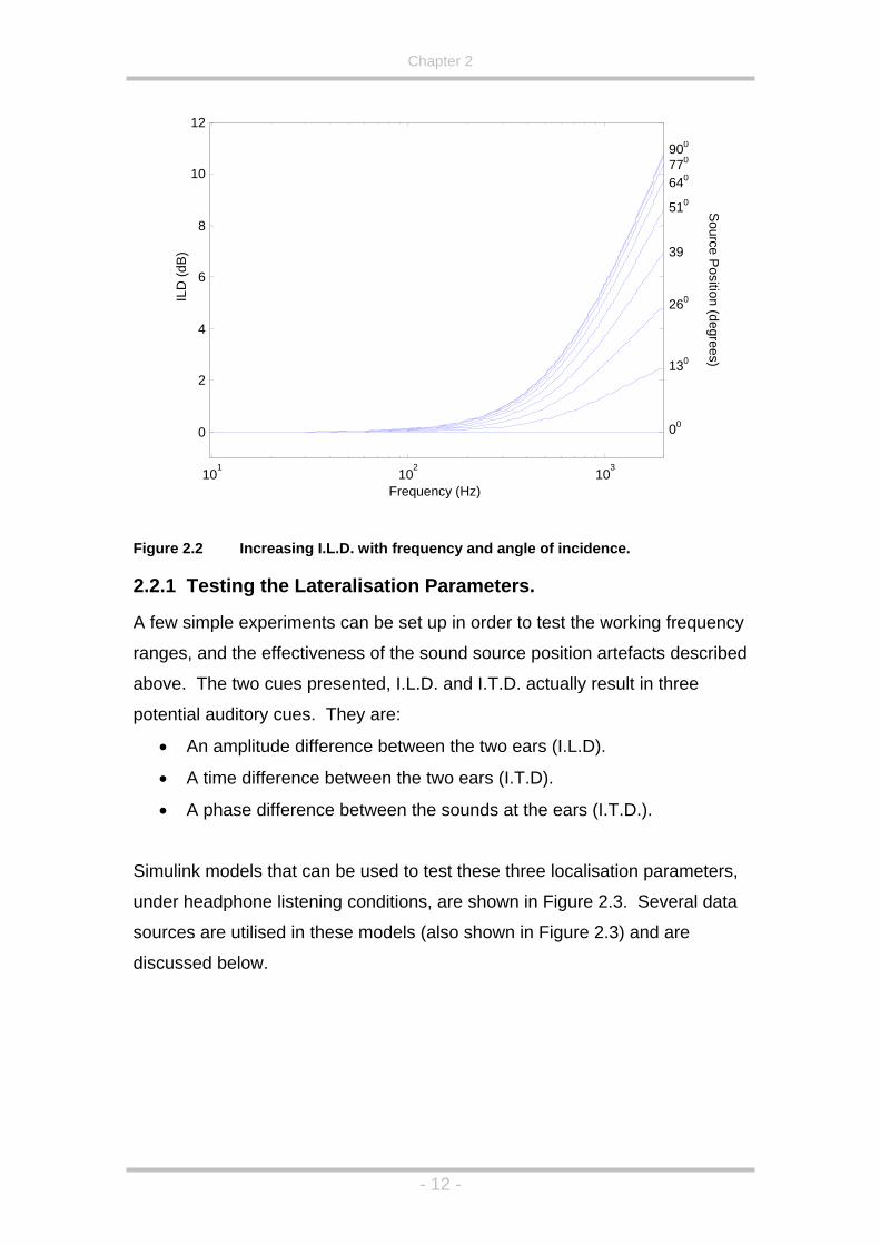
2 kHz, is shown in Figure 2.2 (equations taken from Duda (1993)). This figure
shows the increasing I.L.D. with increasing frequency and angle of incidence.
- 11 -
Chapter 2
10 1 102
103
0
2
4
6
8
10
12
Frequency (Hz)
ILD
(dB
)
00
130
260
39
510
640770900
Source P
osition (degrees)
Figure 2.2 Increasing I.L.D. with frequency and angle of incidence.
2.2.1 Testing the Lateralisation Parameters.
A few simple experiments can be set up in order to test the working frequency
ranges, and the effectiveness of the sound source position artefacts described
above. The two cues presented, I.L.D. and I.T.D. actually result in three
potential auditory cues. They are:
• An amplitude difference between the two ears (I.L.D).
• A time difference between the two ears (I.T.D).
• A phase difference between the sounds at the ears (I.T.D.).
Simulink models that can be used to test these three localisation parameters,
under headphone listening conditions, are shown in Figure 2.3. Several data
sources are utilised in these models (also shown in Figure 2.3) and are
discussed below.
- 12 -

Chapter 2
0 2 4 6
x 105
0
0.2
0.4
0.6
0.8
1g1 array
0 2 4 6
x 105
-1
-0.5
0
0.5
1g2 array
0 0.5 1 1.5 2 2.5 3 3.5 4 4.5
x 104
-0.5
0
0.5
1 second duration of signal array
Figure 2.3 Simulink models showing tests for the three localisation cues provided by I.L.D. and I.T.D..
Arrays ‘g1’ and ‘g2’ are a rectified sine wave and a cosine wave, and are used
to represent an amplitude gain, a phase change or a time delay. In order for
the various lateralisation cues to be tested, the models must be configured as
described below:
• Level Difference – If ‘g1’ is taken as the gain of the left channel, and a
rectified version of ‘g2’ is used for the gain of the right channel, then the
sound source is level panned smoothly between the two ears, and this is
what the listener perceives, at any given frequency.
• Phase Difference – A sine wave of any phase can be constructed using a
mixture of a sine wave at 00 and a sine wave at 900 (a cosine). So
applying the gains ‘g1’ and ‘g2’ to a sine and a cosine wave which are then
summed, will create a sine wave that changes phase from -Π/2 to Π/2. At
low frequencies this test will tend to pan the sound between the two ears.
However, as the frequency increases the phase difference between the
signals has less effect. For example, at 500 Hz the sounds lateralises
very noticeably. At 1000 Hz only a very slight source movement is
- 13 -

Chapter 2
perceivable and at 1500 Hz, although a slight change in timbre can be
noted, the source does not change position.
• Time Difference – For this test a broad band random noise source was
used so that the sound contained many transients. The source was also
pulsed on and off (see Figure 2.3) so that as the time delay between the
two ears changed the pulsed source would not move significantly while it
was sounding. The time delay was achieved using two fractional delay
lines, using ‘g1’ and a rectified ‘g2’ scaled to give a delay between the ears
varying from –0.8 ms to 0.8 ms (+/- 35 samples at 44.1 kHz), which
roughly represents a source deflection of –900 to 900 from straight ahead.
Slight localisation differences seem to be present up to a higher frequency
than with phase differences, but most of this cue’s usefulness seems to
disappear after around 1000 Hz.
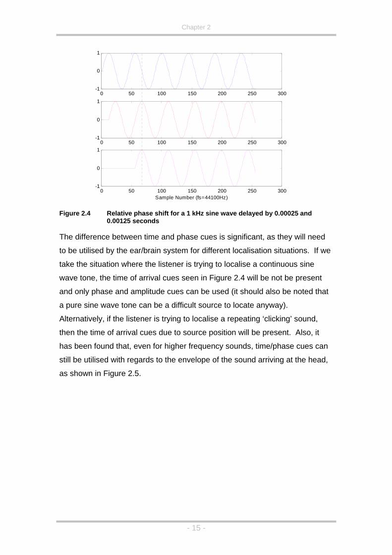
It is clear that the phase and time differences between the two ears of the
listener are related, but they should be considered as two separate cues to
the position of a sound source. For example if we take a 1 kHz sine wave, the
period is equal to 0.001 seconds. If this sound is delayed by 0.00025
seconds, the resulting phase shift will be 900. However, if the sine wave is
delayed by 0.00125 seconds the phase shift seen will be 4500. As the ears
are not able to detect absolute phase shift they must compare the two ears’
signals, which will still give a phase shift of 900 as shown in Figure 2.4. It is
also apparent from Figure 2.4 that if a sound of a different frequency is used,
the same time delay will give a different phase difference between the ears.
As frequency increases the phase change due to path differences between
the ears becomes greater, but once the phase difference between the two
ears is more than 1800 then the brain can no longer decide which signal is
lagging and the cue becomes ambiguous (Gulick, 1989).
- 14 -
Chapter 2
0 50 100 150 200 250 300-1
0
1
0 50 100 150 200 250 300-1
0
1
0 50 100 150 200 250 300-1
0
1
Sample Number (fs=44100Hz)
Figure 2.4 Relative phase shift for a 1 kHz sine wave delayed by 0.00025 and 0.00125 seconds
The difference between time and phase cues is significant, as they will need
to be utilised by the ear/brain system for different localisation situations. If we
take the situation where the listener is trying to localise a continuous sine
wave tone, the time of arrival cues seen in Figure 2.4 will be not be present
and only phase and amplitude cues can be used (it should also be noted that
a pure sine wave tone can be a difficult source to locate anyway).
Alternatively, if the listener is trying to localise a repeating ‘clicking’ sound,
then the time of arrival cues due to source position will be present. Also, it
has been found that, even for higher frequency sounds, time/phase cues can
still be utilised with regards to the envelope of the sound arriving at the head,
as shown in Figure 2.5.
- 15 -

Chapter 2
Figure 2.5 An 8 kHz tone with a low frequency attack envelope
Using a combination of the cues described above, a good indication of the
angle of incidence of an incoming sound can be constructed, but the sound
will be perceived as inside the head with the illusion of sounds coming from
behind the listener being more difficult to achieve. The reason for this is the
so-called ‘Cone of Confusion’ (Begault, 2000). Any sound that is coming from
a cone of directions (shown as grey circles in Figure 2.6) will have the same
level, phase and time differences associated with it making the actual position
of the source potentially ambiguous.
Figure 2.6 Cone of Confusion – Sources with same I.L.D. and I.T.D. are shown as
grey circles.
- 16 -

Chapter 2
So how does the ear/brain system cope with this problem? There are two
other mechanisms that help to resolve the position of a sound source. They
are:
• Head movement.
• Angular dependent filtering.
Head movement can be utilised by the ear/brain system to help strengthen
auditory cues. For example if a source is at 450 to the left (where 00
represents straight ahead), then turning the head towards the left would
decrease the I.L.D. and I.T.D. between the ears and turning the head to the
right would increase the I.L.D. and I.T.D. between the ears. If the source
were located behind the listener the opposite would be true, giving the
ear/brain system an indication of whether the source is in the front or the back
hemi-sphere. In a similar fashion, up/down differentiation can also be
resolved with a tilting movement of the head. This is a very important cue in
the resolution of front/back reversals perfectly demonstrated by an experiment
carried out by Spikofski et al. (2001). In this experiment a subject listens to
sounds recorded using a fixed dummy head with small microphones placed in
its ears. Although reported lateralisation was generally good, many front back
reversals are present for some listeners. The same experiment is then
conducted with a head tracker placed on the listeners head which controls the
angle that the dummy head is facing (that is, the recording dummy head
mirrors the movements of the listener in real-time). In this situation virtually
no front/back reversals are perceived by the listener. Optimising binaural
presentations by utilising the head turning parameter is well documented,
however, its consideration in the optimisation of speaker based systems has
not been attempted, but will be investigated in this project.
Angular dependant filtering is another cue used by the ear/brain system, and
is the only angular direction cue that can be utilised monaurally, that is, sound
localisation can be achieved by using just one ear (Gulick, 1989). The filtering
results from the body and features of the listener, the most prominent of which
is the effect of the pinnae, the cartilage and skin surrounding the opening to
the ear canal, as shown in Figure 2.7.
- 17 -

Chapter 2
Figure 2.7 The Pinna
The pinna acts as a very complex filtering device, imprinting a unique phase
and frequency response onto pressure waves impinging on the head,
depending on the angular direction of this pressure wave. This implies that
sound sources made up of certain bands are more likely to be heard as
emanating from a particular location due to the natural peaks and troughs that
are apparent in the HRTF data due to pinna filtering, and this has been shown
in experiments using narrow-band sound sources. For example, Zwicker &
Fastl (1999) found that narrow band sources of certain frequencies are
located at certain positions on the median plane, irrespective of the position of
the sound source as indicated in Table 2.1.
Narrow band source
centre frequency
Perceived position (in
the median plane)
300Hz, 3kHz Front
8kHz Above
1kHz, 10kHz Behind Table 2.1 Table indicating a narrow band source’s perceived position in the
median plane, irrespective of actual source position.
The example filters shown in Figure 2.8 (taken from HRTF data measured at
the MIT media lab by Gardner & Martin (1994)) shows the phase/magnitude
response at the right ear due to a source at 00,450 and 900 to the right of the
listener. Interestingly, if the complex filtering from a moving source is heard
from a stationary sound source using both ears (e.g. if an in-ear recording is
replayed over speakers), the listener will perceive timbral changes in the
heard material.
- 18 -

Chapter 2
Figure 2.8 Frequency and phase response at the right ear when subjected to an
impulse at 00,450 and 900 to the right of the listener.
Using the points discussed above, a number of simple assumptions can be
made about the human auditory system.
• Amplitude differences between the ears will only be present, and
therefore can only be utilised, in sounds greater than some frequency
(that is, when the sound no longer diffracts around the head).
• Phase cues can only be totally unambiguous if the sound is delayed by
less than half the corresponding wavelength of the sound’s frequency
(i.e. low frequencies), but may still be utilised together with other cues
(such as I.L.D.) up to a delay corresponding to a full wavelength (a
phase change of 3600) (Gulick, W.L. et al., 1989).
• Time cues can only be useful when transients are apparent in the
sound source, e.g. at the beginning of a sound.
2.2.2 Analysis of the Lateralisation Parameters
In order to quantify what frequency ranges the lateralisation parameters are
valid for, an example ‘head’ is now used. This head was measured at the
M.I.T. media lab in the U.S.A. and the impulse response measurements for a
great many source positions were taken in an anechoic room. The resulting
impulse responses are measures of the Head Related Transfer Function
- 19 -

Chapter 2
(which result in Head Related Impulse Responses, but are still generally
known as HRTFs) due to the dummy head. As the tests were carried out in
an anechoic chamber, they are a very good measure of how we lateralise
sound sources, that is, the minimum of auditory cues are present as no
information regarding the space in which the recordings are made is apparent.
Figure 2.9 shows a plot representing the amplitude difference (z-axis)
measured between the two ears for frequencies between 0 Hz and 20 kHz (x-
axis) and source angles between 0 and 1800 (y-axis). The red colouring
indicates that there is no amplitude difference between the ears, and is most
apparent at low frequencies, which is expected as the head does not obstruct
the sound wave for these, longer, wavelengths. The amplitude differences in
the signals arriving at the ears can be seen to occur at around 700 Hz and
then can be seen to increase after this point. This graph shows a significant
difference between modelling the head as a sphere (as in Figure 2.2) and
measuring the non-spherical dummy head with amplitude peaks and troughs
becoming very evident.
Figure 2.9 The relationship between source incidence angle, frequency and
amplitude difference between the two ears.
- 20 -
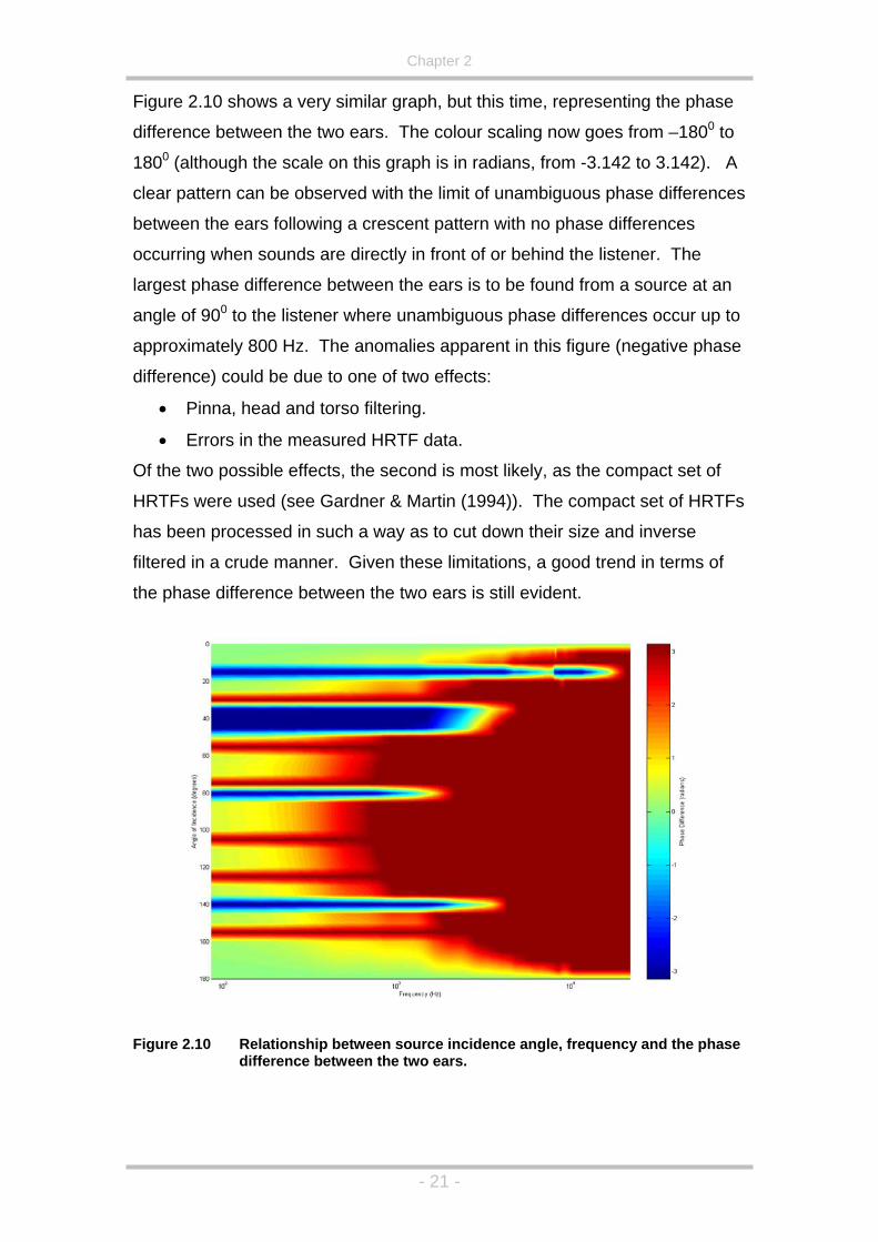
Chapter 2
Figure 2.10 shows a very similar graph, but this time, representing the phase
difference between the two ears. The colour scaling now goes from –1800 to
1800 (although the scale on this graph is in radians, from -3.142 to 3.142). A
clear pattern can be observed with the limit of unambiguous phase differences
between the ears following a crescent pattern with no phase differences
occurring when sounds are directly in front of or behind the listener. The
largest phase difference between the ears is to be found from a source at an
angle of 900 to the listener where unambiguous phase differences occur up to
approximately 800 Hz. The anomalies apparent in this figure (negative phase
difference) could be due to one of two effects:
• Pinna, head and torso filtering.
• Errors in the measured HRTF data.
Of the two possible effects, the second is most likely, as the compact set of
HRTFs were used (see Gardner & Martin (1994)). The compact set of HRTFs
has been processed in such a way as to cut down their size and inverse
filtered in a crude manner. Given these limitations, a good trend in terms of
the phase difference between the two ears is still evident.
Figure 2.10 Relationship between source incidence angle, frequency and the phase
difference between the two ears.
- 21 -
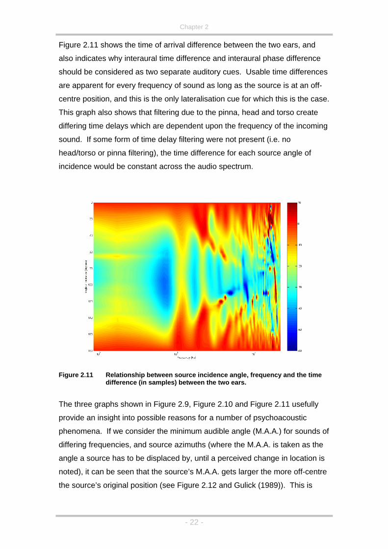
Chapter 2
Figure 2.11 shows the time of arrival difference between the two ears, and
also indicates why interaural time difference and interaural phase difference
should be considered as two separate auditory cues. Usable time differences
are apparent for every frequency of sound as long as the source is at an off-
centre position, and this is the only lateralisation cue for which this is the case.
This graph also shows that filtering due to the pinna, head and torso create
differing time delays which are dependent upon the frequency of the incoming
sound. If some form of time delay filtering were not present (i.e. no
head/torso or pinna filtering), the time difference for each source angle of
incidence would be constant across the audio spectrum.
Figure 2.11 Relationship between source incidence angle, frequency and the time
difference (in samples) between the two ears.
The three graphs shown in Figure 2.9, Figure 2.10 and Figure 2.11 usefully
provide an insight into possible reasons for a number of psychoacoustic
phenomena. If we consider the minimum audible angle (M.A.A.) for sounds of
differing frequencies, and source azimuths (where the M.A.A. is taken as the
angle a source has to be displaced by, until a perceived change in location is
noted), it can be seen that the source’s M.A.A. gets larger the more off-centre
the source’s original position (see Figure 2.12 and Gulick (1989)). This is
- 22 -

Chapter 2
coupled with the M.A.A. increasing for all source positions between the
frequencies of 1 kHz and 3 kHz.
The question arises; can the M.A.A. effect be explained using the three
H.R.T.F. analysis figures given above? Firstly, why would the minimum
audible angle be greater the more off-centre the sound source for low
frequencies? If the phase difference graph is observed, then it can be seen
that the gradient of the change of phase difference with respect to head
movement is greatest when a source is directly behind or directly in front of
the listener. That is, if the head is rotated 10, then a source directly in front of
the listener will create a greater phase change between the two listening
conditions when compared to a source that is at an azimuth of 900 implying an
increased resolution to the front (and rear) of the listener.
500 1000 5000 100000
2
4
6
8
10
12
14
Frequency (Hz)
Min
imum
Aud
ible
Ang
le (d
egre
es)
0 Degrees30 Degrees60 Degrees
Figure 2.12 Minimum audible angle between successive tones as a function of
frequency and position of source (data taken from Gulick (1989)).
It should also be noted that the M.A.A. worsens between 1 kHz and 3 kHz. If
the interaural amplitude is studied, it can be seen that the difference between
the ears starts to become pronounced after approximately 1 kHz and does not
become more obvious until higher frequencies. Also, 1 kHz is around the
frequency where unambiguous phase cues start to disappear (and more so as
the angle of incidence of the source increases). It is this cross-over period
between the brain using level and phase cues where the M.A.A. is at its
- 23 -

Chapter 2
largest. Another interesting result, that can also be seen from Figure 2.12, is
that phase cues (used primarily at low frequencies) perform better, on
average, than higher frequency cues (pinna filtering and level differences) and
it is often mentioned that low frequency, temporal, cues are the more robust
cues (for example, Wightman, F.L. and Kistler, D.J., 1992 and Huopaniemi, J.
et al, 1999).
2.3 Sound Localisation
The term localisation differs from lateralisation in that not only is source
direction angle arrived at, but a listener can gain information on the type of
location a sound is emanating from and the distance from the source to the
listener. Also, information on the size of a sound source as well as which way
it may be facing can be gleaned just by listening for a short time.
2.3.1 Room Localisation
When walking into an acoustic space for the first time, the brain quickly makes
a number of assumptions about the listening environment. It does this using
the sound of the room (using any sounds present) and the reaction of the
listener inside this room. One example of this is when walking into a
cathedral. In this situation one of the first sounds possibly heard will be your
own footsteps, and this will soon give the impression that the listener is in a
large, enclosed space. This is also the reason that people susceptible to
claustrophobia are ill advised to enter an anechoic chamber, as the lack of
any reverberation in the room can be very disconcerting, and bring on a
claustrophobic reaction. Interestingly, listening to sound sources in an
anechoic chamber will often give the impression that the sound source is
almost ‘inside the head’ (much like listening to conventional sound sources
through headphones). The human brain is not used to listening to sounds
without a corresponding location (even large open expanses have sound
reflections from the floor), and the only time this will happen is if the source is
very close to the head, somebody whispering in your ear, for example, and so
the brain decides that any sound without a location is likely to be very close.
- 24 -

Chapter 2
If we are listening to a sound source in a real location, a large number of
reflections may also reach the ears. The first sound that is heard will be the
direct sound, as this has the shortest path length (assuming nothing obstructs
the source). Then, the first order reflections will be heard. Figure 2.13 shows
a simplified example of this (in two dimensions). Here it can clearly be seen
that the direct sound has the shortest path length, which implies that this
signal has the properties listed below:
• The direct sound will be the loudest signal from the source to reach the
listener (both due to the extra path length and the fact that some of the
reflected source’s energy will be absorbed by the reflective surface).
• The direct sound will be the first signal to reach the ears of the listener.
• The direct sound may be the only signal that will be encoded (by the
head of the listener) in the correct direction.
0 0.2 0.4 0.6 0.8 10
0.1
0.2
0.3
0.4
0.5
0.6
0.7
0.8
0.9
1
Source →
← ListenerDirectSound
1st OrderReflections
2nd OrderReflections
Figure 2.13 Simple example of a source listened to in a room. Direct, four 1st order
reflections and one 2nd order reflection shown (horizontal only).
In the example shown above (Figure 2.13) a simple square room is shown
along with four of the 1st order sound reflections (there are two missing, one
from the floor and one from the ceiling) and one 2nd order reflection. These
signal paths will also be attenuated due to absorption associated with the wall
and the air. Surfaces in a room, and the air itself, possess an absorption
coefficient, a numerical grade of acoustic absorption, although a more
- 25 -

Chapter 2
accurate measure is the frequency dependent absorption coefficient. As
reflections in the room build up to higher and higher orders, a diffuse sound
field is created, where the individual echoes are more difficult to analyse.
Figure 2.14 shows an example impulse response of an actual room. The
room has a reasonably short reverberation time as the walls are acoustically
treated with foam panels. The graph shows ¼ of a second in time (11025
samples at 44.1 kHz sampling rate).
0 2000 4000 6000 8000 10000 12000-8
-6
-4
-2
0
2
4
6
8
10x 10-3
Sample Number
Am
plitu
de
Direct Sound
Early, discrete Reflections
Diffuse Tail
Figure 2.14 Impulse response of an acoustically treated listening room.
As mentioned at the beginning of this section, the response of a room gives
listeners significant insight into the type of environment that they are in.
However, Figure 2.14 shows a very complicated response. So how does the
brain process this? An extremely important psychoacoustic phenomenon and
one that the ear/brain system uses in this type of situation has been termed
the precedence effect (Begault, 2000). The precedence effect is where the
brain gives precedence to the sound arriving at the listener first, with the
direction of this first sound taken as the angular direction indicator. This
sounds very simple, but as we have two ears, the initial sound arrives at the
ears twice and, therefore, has two arrival times associated with it. Figure 2.15
shows the equivalent reverberation impulse responses that arrive at both
ears. The source used in this graph is at 300 to the left of the listener very
- 26 -

Chapter 2
close to the rear wall, and about 1 metre away from the left wall. It can clearly
be seen that the source’s direct sound arrives at the left ear first, followed,
around 11 samples later (0.25 ms at 44.1 kHz), by the right ear. As the
ear/brain system uses this time difference to help lateralise the incoming
sound, the precedence effect does not function for such short time
differences. Under laboratory tests it has been noted that if the same signal is
played into each ear of a pair of headphones, but one channel is delayed
slightly (Begault, 2000):
• For a delay between 0 and 0.6mS the source will move from the centre
towards the undelayed side of the listeners head.
• Between approximately 0.7 and 35mS the source will remain at the
undelayed side of the listeners head, that is, the precedence effect
employs the first source to determine the lateralisation. However,
although the source position will not change, the perceived tone, and
width of the source will tend to alter as the delay between the left and
right ears is increased (note that this implies an effect analogous to
comb filtering which occurs during the processing of the sounds
arriving at the two ears by the brain of the listener).
• Finally, increasing the time delay still further will create the illusion of
two separate sources one to the left of the listener and one to the right.
The delayed source is perceived as an echo.
- 27 -

Chapter 2
0 200 400 600 800 1000 1200 1400 1600 1800 2000-0.05
-0.04
-0.03
-0.02
-0.01
0
0.01
0.02
0.03
Sample Number
Am
plitu
de
Left Ear
0 200 400 600 800 1000 1200 1400 1600 1800 2000-0.04
-0.03
-0.02
-0.01
0
0.01
0.02
Sample Number
Am
plitu
de
Right Ear
Figure 2.15 Binaural impulse response from a source at 300 to the left of the
listener. Dotted lines indicate some discrete reflections arriving at left ear.
The above points help to explain why the ear/brain system uses the
precedence effect. If a source has many early reflections (i.e. the source is in
a reverberant room) the ear/brain system needs a way of discriminating
between the direct sound and the room’s response to that sound (reflections
and diffuse field). The precedence effect is the result of this phenomenon. If
we take a source in a room (as given in figure 2.13), assuming the room is a 4
m by 4 m, square room and the initial source is 0.45m away from the listener
(that is, the listener and source positions are as in Figure 2.13). The direct
sound will take 1.3ms to reach the listener (taking the speed of sound in air as
342 ms-1). The source is at an azimuth of approximately 630 from straight
ahead which will lead to a time difference between the ears of around 0.5 ms
(using the approximate binaural distance equation from Gulick (1989)). The
nearest reflection has a path length of around 3.2 m from the source to the
listener which equates to a delay time of 9.4 ms. Because of the precedence
effect, the first time delay between the ears will be utilised in the lateralisation
of the sound source, and the first discrete echo will not be heard as an echo,
but it will not change the perceived position of the sound source either, and
- 28 -

Chapter 2
will just change the width or timbre of the source. It is this type of processing
in the ear/brain system that gives us vital information about the type of space
we are situated in. However, as the above points suggest, it may be at the
expense of localisation accuracy, with the precedence effect breaking down if
the echo is louder than the direct sound, which normally only occurs if the
source is out of sight, but a reflection path off a wall is the loudest sound to
reach the listener.
2.3.2 Height and Distance Perception
Although lateralisation has been discussed, no explanation has yet been
given to resolution of sources that appear above or below the listener. As the
ears of the listener are both on the same plane, horizontally, the sound
reaching each ear will not contain any path differences due to elevation
(although, obviously, if a sound is elevated and off-centre, the path
differences for the lateral position of the sound will be present), and as there
are no path differences the only static cue that can be utilised for an elevated
cue is the comb filtering introduced by head and pinna. Figure 2.16 shows a
3-axis graph representing a source straight in front of the listener changing
elevation angle from –400 to 900. Perhaps the most notable feature of this
plot is the pronounced trough that originates at around 7 kHz for an elevation
of –400, which goes through a smooth transition to around 11 kHz at an
elevation of 600. It is most probably these pinna filtering cues (combined with
head movements) that are used to resolve sources that are above and below
the listener (Zwicker & Fastl, 1999). Interestingly, it has also been shown in
Zwicker & Fastl (1999) that narrow, band-limited sources heard by a listener
can have a ‘natural’ direction. For example, an 8 kHz centre frequency is
perceived as coming from a location above the head of the subject, whereas a
1 kHz centre frequency is perceived as coming from a location behind the
listener.
- 29 -

Chapter 2
Figure 2.16 Relationship between source elevation angle, frequency and the
amplitude at an ear of a listener (source is at an azimuth of 00).
In order to assess the apparent distance of a source to the listener, a number
of auditory cues are used. The first and most obvious cue is that of
amplitude. That is, a source that is near by will be louder than a source that is
further away. The relationship between a point source’s amplitude and
distance, in the free field, is known as the inverse square law as for each
doubling of distance, the amplitude of the source will reduce by a quarter
(1/[22]). This is, of course, the simplest case, only holding true for a point
source in the free field. Sources are rarely a perfect point source, and rarely
heard in the perfect free field (i.e. anechoic circumstances) so, in reality, the
amplitude reduction is normally less than the inverse square law suggests. In
addition to the pure amplitude changes, distance dependant filtering can be
observed, due to air absorption (Savioja, 1999). This will result in a more low-
pass filtered signal, the further away the source. The direct to reverberant
ratio of the sound will change depending on the source’s distance to the
listener with a source close to the listener exhibiting a large amount of direct
sound when compared to the reverberation, but a sound further away will
have a similar amount of reverberation, but a lower level of direct sound
- 30 -

Chapter 2
(Begault, 2000). There are two reasons for this. Firstly, the diffuse part of the
room’s response (i.e. the part not made up of direct sound or first order
reflections) is made up from the sound bouncing off many surfaces, and as
such, will be present all through the room. This means that the level of this
part of the reverberation is reasonably constant throughout the room. Also, as
the source moves away from the listener, the distance ratio between the path
length of the direct sound and the early reflections becomes closer to one.
This means that the first reflections will arrive closer (in time), and have an
amplitude that is more similar to the level of the direct sound. This is shown in
Figure 2.17.
Figure 2.17 A graph showing the direct sound and early reflections of two sources
in a room.
Evidence suggests that the reverberation cue is one of the more robust cues
in the simulation of distance and has been shown to create the illusion of a
sound source outside of the head under headphone listening conditions
(McKeag & McGrath, 1997).
Of all the cues available to differentiate source distances, the least apparent is
that the source’s incidence angle from the listener’s ears will change as the
source is moved away from a listener (Gulick, 1989). Figure 2.18 shows two
source examples, one source very close to the listener, and one source at
- 31 -
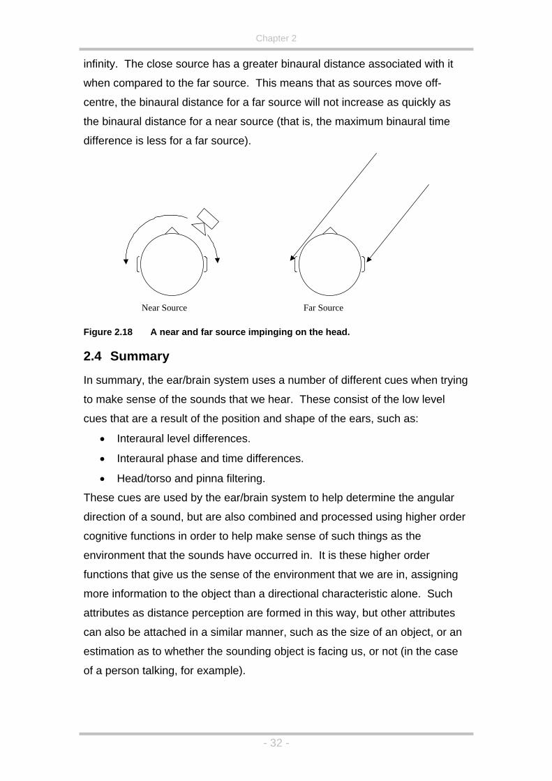
Chapter 2
infinity. The close source has a greater binaural distance associated with it
when compared to the far source. This means that as sources move off-
centre, the binaural distance for a far source will not increase as quickly as
the binaural distance for a near source (that is, the maximum binaural time
difference is less for a far source).
Near Source Far Source
Figure 2.18 A near and far source impinging on the head.
2.4 Summary
In summary, the ear/brain system uses a number of different cues when trying
to make sense of the sounds that we hear. These consist of the low level
cues that are a result of the position and shape of the ears, such as:
• Interaural level differences.
• Interaural phase and time differences.
• Head/torso and pinna filtering.
These cues are used by the ear/brain system to help determine the angular
direction of a sound, but are also combined and processed using higher order
cognitive functions in order to help make sense of such things as the
environment that the sounds have occurred in. It is these higher order
functions that give us the sense of the environment that we are in, assigning
more information to the object than a directional characteristic alone. Such
attributes as distance perception are formed in this way, but other attributes
can also be attached in a similar manner, such as the size of an object, or an
estimation as to whether the sounding object is facing us, or not (in the case
of a person talking, for example).
- 32 -

Chapter 2
If a successful surround sound system is to be developed then it is apparent
that not only should the low-level cues be satisfied, but they should also be as
coherent with one another as possible so that the higher order cognitive
functions of the ear/brain system can also be satisfied in a useful and
meaningful way.
- 33 -

Chapter 3
Chapter 3 - Surround Sound Systems
3.1 Introduction
In this chapter past and current surround sound algorithms and techniques
will be discussed starting with a historical account of the first systems,
proposed by Bell Labs and Alan Blumlein, how Blumlein’s early system was
used as a loose basis for stereo, and then on to the theory and rationale
behind the systems that are used presently.
The early systems are of importance as most surround sound systems in use
today base themselves on the techniques and principles of this early work. In
the context of this research, one main system will be decided upon as
warranting further research in order to fulfil the research problem detailed in
Chapter 1, with the following criteria needing to be met:
• A hierarchical carrier format must be decided upon.
• This carrier must be able to be decoded for multi-speaker systems
with different speaker arrangements.
• This decode must be able to provide the listener with the relevant
auditory cues which will translate well into a binaural representation.
As the above system is to be converted into a binaural and transaural
representation, these systems will also be discussed.
3.2 Historic Review of Surround Sound Techniques and Theory
Although standard stereo equipment works with two channels, early work was
not necessarily fixed to that number, with the stereo arrangement familiar to
us today not becoming a standard until the 1950s. Bell labs original work was
predicated on many more speakers than this initially (Rumsey & McCormick,
1994) and is the first system described in this section.
3.2.1 Bell Labs’ Early Spaced Microphone Technique
The early aims of the first directional sound reproduction techniques tried at
Bell Labs was that of trying to reproduce the sound wave front from a source
- 34 -

Chapter 3
on a stage (Rumsey & McCormick, 1994). A sound source was placed on a
stage in a room; this was then picked up by a large number of closely spaced
microphones in a row, in front of the source. These signals were then
transmitted to an equal number of similarly spaced loudspeakers (as shown in
Figure 3.1).
Source
Figure 3.1 Graphical depiction of early Bell Labs experiments. Infinite number of
microphones and speakers model.
The result was an accurate virtual image that did not depend on the position
of the listener (within limits) as the wave front approaching the speakers is
reproduced well, much like wave-field synthesis (to be discussed later in this
chapter). Bell Labs then tried to see if they could recreate the same idea
using a smaller number of speakers (Figure 3.2), but this did not perform as
accurately (Steinberg, J. & Snow, W., 1934). The main problem with such a
setup is that once the many speakers are removed, the three sources (as in
the example shown in Figure 3.2) do not reconstruct the wave front correctly.
Let us consider the three speaker example shown in Figure 3.2. If the source
is recorded by three microphones, as shown, the middle microphone will
receive the signal first, followed then by the microphone on the right, and
lastly captured by the microphone on the left. These three signals are
reproduced by the three loudspeakers. If the listener is placed directly in front
of the middle loudspeaker, then the signal from the middle speaker will reach
them first, followed by the right and left loudspeakers together. However, as
the signal from the source was delayed in reaching the left and right
- 35 -

Chapter 3
microphones, the delay from each of the left and right speakers is increased
even more. Now, if the combined spacing between the microphones and
speakers equates to a spacing greater than the diameter of the head, then the
time delays reproduced at the ears of the listener will be greater than the
maximum interaural time difference of a real source. This will then result in
either the precedence effect taking over (i.e. the source will emanate from the
centre loudspeaker) or, worse still, echoes will be perceived. This is due to a
phenomenon known as ‘spatial aliasing’ and will be described in more detail in
section 3.3.2. The spacing of the microphones was necessary as directional
microphones had not been invented at this point in time, and only pressure
sensitive, omnidirectional microphones were available.
Source
Figure 3.2 Early Bell Labs experiment. Limited number of microphones and
speakers model.
3.2.2 Blumlein’s Binaural Reproduction System
While carrying out research into the work of Alan Blumlein, it was soon
discovered that there seems to be some confusion, in the audio industry,
about certain aspects of his inventions. This seems mainly due to the fact
that the names of the various techniques he pioneered have been changed,
or misquoted, from the names that he originally gave. Alan Blumlein delivered
a patent specification in 1931 (Blumlein, 1931) that both recognised the
problems with the Bell Labs approach and defined a method for converting
spaced microphone feeds to a signal suitable for loudspeaker reproduction.
Blumlein called his invention Binaural Reproduction. This recording technique
comprised of two omni-directional microphones spaced at a distance similar
- 36 -

Chapter 3
to that found between the ears, with a round panel baffle in between them.
This technique was known to work well for headphone listening, but did not
perform as accurately when replayed on loudspeakers. Blumlein realised that
for loudspeaker reproduction, phase differences at the speakers (i.e. in the
spaced microphone recording) did not reproduce phase differences at the
listener’s ears. This was due to the unavoidable crosstalk between the two
speakers and the two ears of the listener, as shown in Figure 3.3.
x x
Figure 3.3 Standard “stereo triangle” with the speakers at +/-300 to the listener (x denotes the crosstalk path).
Blumlein had discovered that in order to reproduce phase differences at the
ears of a listener, level differences needed to be presented by the speakers.
His invention included the description of a ‘Shuffling’ circuit, which is a device
that converts the phase differences, present in spaced microphone
recordings, to amplitude differences at low frequencies (as at higher
frequencies the amplitude differences would already be present due to the
sound shadow presented by the disk between the two microphones).
If we consider the stereo pair of loudspeakers shown in Figure 3.3, it can be
seen that there are two paths from each speaker to each ear of the listener. If
the sound that is recorded from the Blumlein stereo pair of microphones is to
the left of centre, then the left channel’s signal will be greater in amplitude
than the right channel’s signal. Four signals will then be transmitted to the
ears:
1. The left speaker to the left ear.
- 37 -

Chapter 3
2. The left speaker to the right ear.
3. The right speaker to the right ear.
4. The right speaker to the left ear.
If we take the case of a low frequency sound (where the interaural phase
difference is the major cue), as the paths from the speaker to the contralateral
ear is longer than from the speaker to the ipsilateral ear, the signal will appear
delayed in time (but not changed in amplitude, due to the wave diffracting
around the head, see Chapter 2). The resulting signals that arrive at each ear
are shown in Figure 3.4.
Figure 3.4 Low frequency simulation of a source recorded in Blumlein Stereo and
replayed over a pair of loudspeakers. The source is to the left of centre.
It can be clearly seen that low frequency phase cues can be encoded into a
stereo signal using just amplitude differences and once the head starts to
become a physical obstacle for the reproduced signals (at higher
frequencies), a level difference between the ears will also become apparent.
It may seem strange that Blumlein used a spaced microphone array to model
what seems to be a coincident, amplitude weighted, microphone technique,
but only omnidirectional microphones were available at this time. However,
less than a year later a directional, ribbon microphone appeared that had a
figure of eight polar response. This microphone was better suited to
Blumlein’s Binaural Reproduction technique.
- 38 -

Chapter 3
Figure 3.5 Polar pickup patterns for Blumlein Stereo technique
Blumlein’s coincident microphone technique involved the use of two
coincident microphones with figure of eight pickup patterns (Blumlein, 1931)
(as shown in Figure 3.5) and has a number of advantages over the spaced
microphone set-up shown in Figure 3.2. Firstly, this system is mono
compatible, whereas spaced microphone techniques are generally not (if not
shuffled). If we again consider the microphone arrangement given in Figure
3.2 then each of the microphones receives the same signal, but changed in
delay and amplitude. As there are delays involved, adding up the different
channels will produce comb-filtering effects (as different frequencies will
cancel out and reinforce each other depending on their wavelengths).
However, this will not be the case using Blumlein’s binaural sound as the two
microphones will pick up the same signal, differing only in amplitude. A mono
signal can be constructed by adding the left and right signals together
resulting in a forward facing figure of eight response. The Blumlein approach
also has the added advantage that the actual signals that are presented from
each loudspeaker can be altered after the recording process. For example,
the apparent width of the sound stage can be altered using various mixtures
of the sum and difference signals (see spatial equalisation, later in this
section). Also, Blumlein based his work on what the ear would hear, and
- 39 -

Chapter 3
described how a stereo image, made up of amplitude differences alone, could
create low frequency phase cues at the ears of a listener (Blumlein, 1931).
Blumlein did foresee one problem with his two microphone arrangement,
however. This was that the amplitude and phase cues for mid and low
frequencies, respectively, would not be in agreement (Blumlein, 1931;
Glasgal, 2003a). It was possible to solve this problem using the fact that the
signals fed to each speaker could be altered after recording using the sum
and difference signals. This technique is now known as spatial equalisation
(Gerzon, 1994), and consisted of changing the low frequency signals that fed
the left and right speaker by boosting the difference signal and cutting the
sum signal by the same amount (usually around 4dB). This has the effect of
altering the pickup pattern for the recorded material in a manner shown in
Figure 3.6. This technique is still used today, and is a basis for parts of the
Lexicon Logic 7™ (Surround Sound Mailing List Archive, 2001) and
Ambisonic systems (Gerzon, 1974), the principles of which will be discussed
in detail later in this chapter.
Figure 3.6 Graph showing the pick up patterns of the left speaker’s feed after
spatial equalisation.
Blumlein’s binaural reproduction technique is one of the few that truly
separates the encoding of the signal from the decoding, which allows for the
various post recording steps that can be carried out in a clearly defined,
- 40 -

Chapter 3
mathematically elegant way. Blumlein was soon employed by the military to
work on radar, amongst other things. It may be because of this that
Blumlein’s work was not openly recognised for a number of years (Alexander,
1997), but his principles were later used in the formulation of a three
dimensional sound system (see Ambisonics, later in this chapter).
3.2.3 Stereo Spaced Microphone Techniques
Although the Blumlein Stereo technique has many advantages as a recording
format when used for reproduction over loudspeakers, there is another school
of thought on this matter. This is that such ‘summation localisation theories’
cannot hope to accurately reproduce recorded material as no onset time delay
is introduced into the equation, and if this is the case, then although steady
state (continuous) signals can be reproduced faithfully, the onset of sounds
cannot be reproduced with strong enough cues present to successfully fool
the ear/brain system. To this end, a number of spaced microphone
techniques were developed that circumvented some of the problems
associated with Bell Labs wave front reconstruction technique described
above. It must be noted, however, that Blumlein did use spaced microphone
techniques to record sound as he was well aware that, for headphone
listening, this produced the best results. However, in order to replay these
recordings over speakers, to achieve externalisation, a Blumlein shuffler was
used, that converted the signals, at low frequencies, to consist of only
amplitude differences.
If we recall from the Bell Labs system, anomalies occurred because of the
potentially large spacing between the microphones that were picking up the
sound sources. A more logical approach is a near-coincident microphone
technique that will limit the time of arrival errors so that the maximum time
difference experienced by a listener will not be perceived as an echo. The
ORTF method uses a pair of spaced directional microphones usually spaced
by around 17 cm (roughly equal to the diameter of a human head) and at an
angle of separation of 1100 (as shown in Figure 3.7). This means that the
largest possible time difference between the two channels is comparable with
the largest time of arrival difference experienced by a real listener. Directional
- 41 -

Chapter 3
microphones are used to simulate the shadowing effect of the head. This
arrangement is a trade off between spaced and coincident microphone
techniques as it has the increased spaciousness of spaced microphones (due
to the increased de-correlation of the two signals) but also has reasonably
good mono compatibility due to the close proximity of the microphone
capsules.
1100
17cm
Figure 3.7 ORTF near-coincident microphone technique.
Another widely used technique is the Decca Tree (Rumsey and McCormick,
1994). This is a group of three microphones matrixed together to create two
loudspeaker feeds. An example of the Decca Tree arrangement is shown in
Figure 3.8. In this arrangement the centre microphone feed is sent to both
channels, the left microphone feed is sent to the left channel and the right
microphone is sent to the right channel. In this way, the differences between
the two channels outputs are lessened, giving a more stable central image,
and alleviating the ‘hole in the middle’ type effect of a spaced omni technique
(the sound always seeming to originate from a specific speaker, as in the Bell
Labs set-up).
- 42 -

Chapter 3
1.5m
2m
Figure 3.8 Typical Decca Tree microphone arrangement (using omni-directional capsules).
3.2.4 Pan-potted Stereo
The systems that have been discussed thus far have been able to record
events for multiple speaker playback, but a system was needed that could be
used to artificially place sources in the desired location to create the illusion of
a recorded situation. Due to the simplicity of Blumlein stereo, as opposed to
spaced microphone techniques, creating a system where individual sources
could be artificially positioned was based on amplitude panning (Rumsey and
McCormick, 1994). So, a simulation of the Blumlein coincident microphone
system was needed. As the coincident microphones were figure of eight
responses the gains needed to artificially pan a sound from the left speaker to
the right speaker are given in equation (3.1). The SPos offset parameter is
basically to ‘steer’ the virtual figure-of-eight responses so that a signal at one
speaker position will have no gain at the opposite speaker, i.e. a virtual source
at the speaker position is an actual source at the speaker position.
)cos()sin(
SPosRightGainSPosLeftGain+=
+=θ
θ
(3.1)
where: SPos is the absolute angular position of the speaker.
θ is the desired source position (from SPos0 to –SPos0).
- 43 -

Chapter 3
Figure 3.9 A stereo panning law based on Blumlein stereo.
This is, however, really a simplification of Blumlein’s stereo technique as his
spatial equalisation circuit is generally not used in amplitude stereo panning
techniques.
Simple amplitude (or pair-wise panning) has now been used for many years,
but does suffer from a few problems. It has been shown that the maximum
speaker separation that can be successfully utilised is +/- 300 and that side-
imaging is very hard to achieve using this method (Glasgal, 2003b). Both of
these facts are not necessarily detrimental to simple two-speaker stereo
reproduction, but will present a larger problem with surround sound
techniques as this would mean a minimum of six equally spaced speakers
placed around the speaker would need to be used (based on only the angular
spacing assumption).
In summary, there are basically two schools of thought when it comes to the
recording of live situations for replay over a stereo speaker array (pan-potted,
stereo, material is almost always amplitude panned, although artificial
reverberation devices often mimic a spaced microphone array rather than a
coincident setup). There are those that abide by spaced microphone
techniques, reasoning that the time onset cues are very important to the
- 44 -

Chapter 3
ear/brain system (i.e. the precedence effect) and these are impossible to
recreate using a coincident microphone arrangement. On the other side there
are those who prefer the mathematical simplicity of coincident microphone
arrangements, believing that the potential phase/time misalignment of the
signals originating from the speakers in spaced microphone techniques to be
detrimental to both the timbre and accuracy of the recorded material. Of
course, both are correct to a certain degree and both coincident and spaced
techniques can produce very pleasing results. However, the main problem
with spaced microphone techniques is that, because potentially unknown time
differences will be present between the two channels, the practical
reprocessing of new signal feeds becomes much more difficult, while not an
issue for two-speaker stereo, will become an issue for larger arrays of
speakers.
3.2.5 Enhanced Stereo
As can be deduced from both Blumlein and Bell Labs early work, stereo
sound (which, incidentally, neither Blumlein or Bell Labs referred to their work
as ‘Stereo’ sound) was never limited, theoretically, to just two speakers, as
their work was mainly geared towards film sound reproduction that needed to
encompass large audiences. Three speakers was a good minimum for such
a situation as it was soon found that angular distortion was not too detrimental
to the experience, except when it came to dialogue (Blumlein’s original idea of
the dialogue following the actors was not widely taken up). Dialogue needed
to always sound as if it was coming from the screen and not the nearest
speaker to the listener, which could happen due to the precedence effect. To
this end the centre speaker was useful for both fixing dialogue to the centre of
the sound stage, and also for increasing the useful listening area of the room.
If a source is panned between two speakers, then a mixture of the time
difference and the level difference between the ears will be used to calculate
where the sound source is originating from. So, if the listener is in the centre
of the two speakers the time (phase) cues will be constructed from the level
differences between the speakers. However, as the listener moves off-centre
the time delay from the two speakers will change the perceived direction of
the sound source. This time difference can be counteracted by the amplitude
- 45 -

Chapter 3
differences between the two speakers, but angular distortion will always
occur, and once the listener is much closer to one speaker than the other, all
but the hardest panned material will tend to emanate from the closer of the
two loudspeakers. Hence, having a centre speaker not only fixed dialogue to
the screen, but also lessened the maximum time difference that could be
experienced between two speakers at any one time.
3.2.6 Dolby Stereo
Much of the motivation for early surround sound implementations was the
cinema, and early multi-channel playback was attempted as early as 1939 in
the Disney film, Fantasia (Kay et al. 1998). However, although a magnetic
multi-channel standard had been available since the 1950’s (Dolby Labs,
2002), it was not as robust or long lasting as the mono optical track that was
used at this time. Dolby was to change this in 1975 mainly due to the use of
their noise reduction techniques that had revolutionised the professional
recording industry since the 1960’s. The optical system in use at that time
had a number of problems associated with it. The standard for the mono
track’s frequency response was developed in the 1930’s which, although
making the soundtrack replayable in almost any cinema in the world, reduced
the bandwidth to that of a telephone. This response, called the Academy
characteristic (Dolby Labs, 2002), also meant that the soundtracks were
recorded with so much high frequency pre-emphasis that considerable
distortion was also present in the audio. Dolby’s research found that most of
these problems were because of the low signal to noise ratio of the optical
transmission medium, and in the late 1960’s looked at using their type A noise
reduction systems in order to improve the response of the sound. Although
this worked very well, the noise reduction was not embraced as
enthusiastically as for the professional audio industry and Dolby decided that
if it was to make serious ground in the film industry it was the number of
channels available, and not solely the sound quality that would gain success.
In 1975 Dolby made public their film sound breakthrough. Using the same
optical technology as was already in place, a new four-channel stereo system
was introduced (Dolby Labs, 2002). It worked by storing just two channels of
audio which represented the left and right speaker feeds. Then, the sum of
- 46 -

Chapter 3
these two channels represented the centre channel, and the difference
between these two signals represented the surround feed. These principles
were updated slightly due to the nature of the storage mechanism and replay
situations.
1. Due to the potential phase misalignment and other analogue
imperfections in the replay medium, high frequency sounds intended
for the centre front speaker could leak back into the surround speakers.
For this reason, the surround channels were band limited to around 7
kHz.
2. The surround speakers found in cinemas were often closer to the
listener than the front speakers were. To make sure that the
precedence effect didn’t pull much of the imaging to the back and
sides, the surround feeds were delayed.
3. The surround feed was phase shifted by +/- 900 prior to being added to
the left and right channels. This meant that any material added to the
surround channel would be summed, equally out of phase, with the left
and right channels (as opposed to one in phase, one out of phase).
A simplified block diagram of the Dolby encode/decode process is shown in
Figure 3.10. This, matrix, surround sound technique had a number of points
in its favour:
1. It could be distributed using just two channels of audio
2. It was still an optical, and therefore cheap and robust, recording
method.
3. The stereo track was mono compatible.
4. A new curve characteristic was used which, when coupled with Dolby
noise reduction, greatly improved the fidelity of cinema sound.
For these reasons, the film industry took to the new Dolby Stereo format.
- 47 -

Chapter 3
Left
Right
Centre
Surround
- 3dB
- 3dB
+
+
+
+
Bandpass 100Hz –7Khz
+j
-j
+
+
+
+
Lt
Rt
Left
Right
Centre
Surround
- 3dB - 3dB
- 3dB- 3dB
+
+
+
+
Bandpass 100Hz –7Khz
+j
-j
+
+
+
+
Lt
Rt
Dolby Stereo Encoding Process
Lt
Rt
Left
Right
+
+Centre
+
-
900 Phase Shifter -3dB
Sur Right
Sur Left-1
20mS Delay
Lt
Rt
Left
Right
+
+Centre
+
-
900 Phase Shifter -3dB-3dB
Sur Right
Sur Left-1-1
20mS Delay
Dolby Stereo Decoding Process
Figure 3.10 Simplified block diagram of the Dolby Stereo encode/decode process
3.2.7 Quadraphonics
While Dolby was concentrating on film sound reproduction, surround sound
techniques were being developed for a wider audience (in the home) and the
first of these systems was termed Quadraphonics. Quadraphonics worked on
the principle that if the listener wanted to be surrounded by sound then all that
would be needed was an extension of the stereo panning law described
above, but moving between four loudspeakers. The loudspeakers were setup
in a square (usually) and sounds could theoretically be pair-wise panned to
any azimuth around the listener. However, it was soon shown that +/- 450
was too wide a panning angle at the front and back, and side images could
not be formed satisfactorily using pair-wise panning techniques (Gerzon,
1974b & 1985). This, coupled with a number of incompatible formats, the
extra expense needed for more speakers/amplifiers and the poor performance
of early Quadraphonic matrix decoders meant that Quadraphonics was not a
commercial success.
- 48 -

Chapter 3
3.3 Review of Present Surround Sound Techniques
This section describes systems that are now still generating work and interest
within the surround sound community (not necessarily any newer than some
systems mentioned in section 3.2).
Systems in use today can be separated into two distinct categories:
1. Systems that define a speaker layout and/or carrier medium but
with no reference to how signals are captured and/recorded for the
system. Examples include
o Dolby Digital - Ac-3 (Dolby Labs, 2004)
o DTS (Kramer, N.D.)
o Meridian Lossless packaging (De Lancie, 1998)
2. Systems that define how material is captured and/or panned for
replay over a specified speaker layout. Examples include
o Ambisonics
o Wavefield Synthesis
o Ambiophonics
This thesis will concentrate on the systems in the 2nd of these categories, that
define how material is captured and replayed over a system as the 1st type of
system is just defining a standard for which the 2nd category of system could
be applied to (for example, both DTS and Dolby Digital are both lossy,
perceptual codecs used to efficiently store 6 discrete channels to be played
over a standard, ITU, 5.1 speaker array)
3.3.1 Ambisonics
3.3.1.1 Theory
Ambisonics was a system pioneered mainly by Michael Gerzon and is based
on the spherical harmonic decomposition of a sound field (Gerzon, 1974). In
order to understand this last statement the fundamentals of Ambisonics are
reviewed.
A definition for what makes a decoder Ambisonic can be found in Gerzon &
Barton (1992) and their equivalent U.S. patent regarding Ambisonic decoders
- 49 -

Chapter 3
for irregular arrays (Gerzon & Barton, 1998), and states (slightly adapted to
remove equations):
A decoder or reproduction system is defined to be Ambisonic if, for a centrally
seated listening position, it is designed such that:
• The decoded velocity and energy vector angles agree and are
substantially unchanged with frequency.
• At low frequencies (below around 400 Hz) the low frequency
velocity vector magnitude is equal to 1 for all reproduced azimuths.
• At mid/high frequencies (between around 700 Hz and 4 kHz) the
energy vector magnitude is substantially maximised across as large
a part of the 3600 sound stage as possible.
To understand these statements, the underlying concepts of Ambisonics will
be explained, leading into a description of the velocity and energy vectors and
their relevance to multi-speaker surround sound systems.
Ambisonics is a logical extension of Blumlein’s binaural reproduction system
(at least, after it’s conception). Probably one of the most forward looking
features of the Blumlein technique is that when using the two figure of eight
capsules positioned perpendicular to each other, any other figure of eight
response could be created (it was this fact that was utilised in Blumlein’s
spatial equalisation technique). For example, if we take the two figure of eight
microphones shown in Figure 3.5, then any figure of eight microphone
response can be constructed using the equations shown in Equation (3.2).
Some example microphone responses have been plotted in Figure 3.11.
( )( )
( )( ) ( )( )DifSumFigureRLDif
RLSum
×+×=−=
+=
θθ sincos82
2
(3.2)
where: θ is the desired response angle.
L is the left facing figure of eight microphone.
R is the right facing figure of eight microphone.
- 50 -
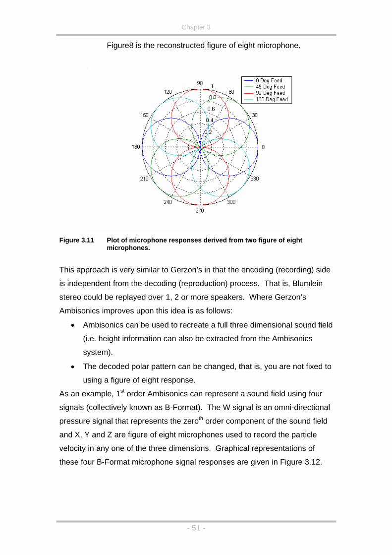
Chapter 3
Figure8 is the reconstructed figure of eight microphone.
Figure 3.11 Plot of microphone responses derived from two figure of eight
microphones.
This approach is very similar to Gerzon’s in that the encoding (recording) side
is independent from the decoding (reproduction) process. That is, Blumlein
stereo could be replayed over 1, 2 or more speakers. Where Gerzon’s
Ambisonics improves upon this idea is as follows:
• Ambisonics can be used to recreate a full three dimensional sound field
(i.e. height information can also be extracted from the Ambisonics
system).
• The decoded polar pattern can be changed, that is, you are not fixed to
using a figure of eight response.
As an example, 1st order Ambisonics can represent a sound field using four
signals (collectively known as B-Format). The W signal is an omni-directional
pressure signal that represents the zeroth order component of the sound field
and X, Y and Z are figure of eight microphones used to record the particle
velocity in any one of the three dimensions. Graphical representations of
these four B-Format microphone signal responses are given in Figure 3.12.
- 51 -

Chapter 3
W
X Y Z
Figure 3.12 The four microphone pickup patterns needed to record first order
Ambisonics (note, red represents in-phase, and blue represents out-of-phase pickup).
Ambisonics is a hierarchical format so that although four channels are needed
for full three-dimensional reproduction, only three channels are needed if the
final replay system is a horizontal only system. The mathematical equations
representing the four microphone responses shown in Figure 3.12 are shown
in equation (3.3). These equations can also be used to encode a sound
source and represent the gains applied to the sound for each channel of the
B-format signal.
( ) ( )( ) ( )( )α
αθαθ
sincossincoscos
21
=×=×=
=
ZYXW
(3.3)
where: α = elevation angle of the source.
θ = azimuth angle of the source.
In order to replay a B-Format signal, virtual microphone responses are
calculated and fed to each speaker. That is, using the B-format signals, any
1st order microphone response can be obtained pointing in any direction. As
mentioned before, this is very much like the theory behind Blumlein Stereo,
except that you can choose the virtual microphone response from any first
- 52 -

Chapter 3
order pattern (and not just a figure of eight), from omni to figure of eight. This
is possible using the simple equation shown in equation (3.4) (Farina et al.,
2001)
( ) ( )( ) ( )( )( ) ( )[ ]ZgYgXgdWgdS
gggg
zyxw
z
y
x
w
+++−×==
===
25.0sin
cossincoscos
2
α
αθαθ
(3.4)
where: W,X,Y & Z are the B-format signals given in equation (3.3)
S = speaker output
θ = speaker azimuth
α = speaker elevation
d = directivity factor (0 to 2)
This gives us the flexibility to alter the polar pattern for each speaker in a
decoder. Example patterns are shown in Figure 3.13.
To clarify the Ambisonic encode/decode process, let us encode a mono
source at an azimuth of 350 and an elevation of 00 and replay this over a six
speaker, hexagonal rig.
- 53 -

Chapter 3
Figure 3.13 Graphical representation of the variable polar patterns available using
first order Ambisonics (in 2 dimensions, in this case).
From equation (3.3) the B-format (W, X, Y and Z) signals will consist of the
amplitude weighted signals shown in equation (3.5).
W = 0.7071 x mono
X = cos(35)cos(0) x mono = 0.8192 x mono
Y = sin(35)cos(0) x mono = 0.5736 x mono
Z = sin(0) x mono = 0 x mono
(3.5)
Where: mono is the sound source to be panned
W, X, Y & Z are the resulting B-Format signals after mono has had the
directionally dependant amplitude weightings applied.
Equation (3.4) can now be used to decode this B-format signal. In this case a
cardioid response will be used for each speaker’s decoded feed, which
equates to a directivity factor of 1 (see Figure 3.13). Equation (3.6) shows an
example speaker feed for a speaker located at 1500 azimuth and 00 elevation.
- 54 -
Chapter 3
S = 0.5 x [(1.414 x W) + (-0.866 x X) + (0.5 x Y) + (0 x Z)]
(3.6)
where: W, X & Y are the encoded B-Format signals.
S = resulting speaker feed
The polar pattern used for the decoder can be decided either by personal
preference, that is, by some form of empirically derived setting, or by a
theoretical calculation which obtains the optimum decoding scheme.
This leads us back to the original statement of what makes a system
Ambisonic. Although the B-format input signal is the simplest to use for the
Ambisonic system, the term Ambisonics is actually more associated with how
a multi-channel decode can be obtained that maximises the accuracy of the
reproduced sound field. The three statements given at the beginning of this
section mention the energy and velocity vectors associated with a multi-
speaker presentation, and it is using these that an Ambisonic decoder can be
designed.
3.3.1.2 Psychoacoustic Decoder Design Using the Energy and Velocity Vectors.
Although Gerzon defined what makes a system Ambisonic, a number of
different decoding types have been suggested both by Gerzon himself and by
others (see Malham, 1998 and Farino & Uglotti, 1998). However, the theory
behind Ambisonics is, as already mentioned, similar to Blumlein’s original idea
that in order to design a psychoacoustically correct reproduction system the
two lateralisation parameters must be optimised with respect to a centrally
seated listener (Gerzon, 1974).
Originally, Gerzon’s work concentrated on regularly spaced arrays in two and
three dimensions (such as square and cuboid arrays) where the virtual
microphone responses chosen for the decoders were based on the system
being quantified using the principles of energy and velocity vectors calculated
at the centre of the array to be designed. These two vectors have been
shown to estimate the perceived localisation and quality of a virtual source
- 55 -
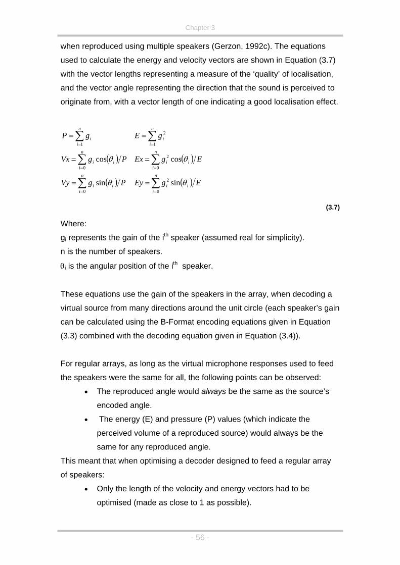
Chapter 3
when reproduced using multiple speakers (Gerzon, 1992c). The equations
used to calculate the energy and velocity vectors are shown in Equation (3.7)
with the vector lengths representing a measure of the ‘quality’ of localisation,
and the vector angle representing the direction that the sound is perceived to
originate from, with a vector length of one indicating a good localisation effect.
( )
( )∑
∑
∑
=
=
=
=
=
=
n
iii
n
iii
n
ii
PgVy
PgVx
gP
0
0
1
sin
cos
θ
θ ( )
( )∑
∑
∑
=
=
=
=
=
=
n
iii
n
iii
n
ii
EgEy
EgEx
gE
0
2
0
2
1
2
sin
cos
θ
θ
(3.7)
Where:
gi represents the gain of the ith speaker (assumed real for simplicity).
n is the number of speakers.
θi is the angular position of the ith speaker.
These equations use the gain of the speakers in the array, when decoding a
virtual source from many directions around the unit circle (each speaker’s gain
can be calculated using the B-Format encoding equations given in Equation
(3.3) combined with the decoding equation given in Equation (3.4)).
For regular arrays, as long as the virtual microphone responses used to feed
the speakers were the same for all, the following points can be observed:
• The reproduced angle would always be the same as the source’s
encoded angle.
• The energy (E) and pressure (P) values (which indicate the
perceived volume of a reproduced source) would always be the
same for any reproduced angle.
This meant that when optimising a decoder designed to feed a regular array
of speakers:
• Only the length of the velocity and energy vectors had to be
optimised (made as close to 1 as possible).
- 56 -

Chapter 3
• This could be achieved by simply changing the pattern control (d) in
equation (3.4) differently for low (<700Hz) and high (>700Hz)
frequencies.
As an example Figure 3.14 shows the velocity and energy vector plots of an
eight speaker horizontal Ambisonic array using virtual cardioid responses for
each speaker feed.
Figure 3.14 Velocity and Energy Vector plot of an eight-speaker array using virtual
ca
rdioids (low and high frequency directivity of d=1).
In order to maximise the performance of this decoder according to Gerzon’s
methods, the low frequency (velocity) vector length should be 1, and the high
frequency (energy) vector length should be as close to 1 as possible (it is
impossible to realise a virtual source with a energy vector of one, as more
than one source is reproducing it). This can be achieved by using a low
frequency directivity pattern of d=1.33 and a high frequency directivity pattern
of d=1.15. This produces the virtual microphone patterns as shown in Figure
3.15 (showing the low frequency pattern for a speaker at 00 and a high
frequency pattern for a speaker at 1800 in order to make each pattern easier
to observe) and has a corresponding velocity and energy vector plot as shown
in Figure 3.16.
-1.5 -1 -0.5 0 0.5 1 1.5
-1
-0.5
0
0.5
D low = 1 : D high = 1
1
Unit Circle
Speakers
Encode Angles
Energy Vectors
Velocity Vectors
Decode Angles
- 57 -

Chapter 3
0.2
0.4
0.6
0.8
1
30
60
270
120
150
210
240 300
330
180 0
90
Virtual microphone response or a 1st order, eight speaker rigs f
HF Polar ResponseLF Polar Response
Figure 3.15 Virtual microphone responses that maximise the energy and velocity
vector responses for an eight speaker rig (shown at 00 and 1800 for clarity).
-1.5 -1 -0.5 0 0.5 1 1.5
-1
-0.5
0
0.5
1
D low = 1.33 : D high = 1.15
e
Y
Figure 3.16 Velocity and Energy Vector plot of an eight speaker Ambisonic decodusing the low and high frequency polar patterns shown in Figure 3.16.
As can be seen in Equation (3.4), a change of polar pattern in the decoding
equation will result in two gain offsets; one applied to the W signal, and
another applied to the X, Y and Z signals. This could be realised,
algorithmically, by the use of shelving filters boosting and cutting the W, X,
- 58 -

Chapter 3
and Z signals by the desired amount prior to decoding, which simplified t
design of, what was at the time, an analogue decoder.
It soon became apparent that, due to both the cinema and proposals for high
definition television, the standard speaker layout for use in the home was not
going to be a regular array. Gerzon had always had difficulty in solving the
velocity and energy vector equations for irregular arrays because irregular
arrays would generally need optimising, not only for the vector lengths, but
also for the decoded source angles and the perceived volume of the decoder
he
(for example, more speakers in the front hemisphere, when compared to the
rear, would cause sources to be louder when in that hemisphere). This meant
that a set of non-linear simultaneous equations needed to be solved. Also,
the shelving filter technique used for regular decoders could not be used for
irregular decoders as it was not just the polar pattern of the virtual
microphones that needed to be altered. To this end a paper was published in
1992 (Gerzon & Barton, 1992) describing how a cross-over filter technique
could be used along with two decoder designs, one for the low frequency and
one for the high frequencies, in order to solve the irregular speaker problem.
In the Gerzon & Barton (1992) paper, a number of irregular Ambisonic
decoders were designed, however, although many five speaker decoder
examples were given, none were as irregular as the ITU finally specified. For
example, the yout are +/- 30 from straight 0 from directly behind the listener, respectively, but the
r
.
front and rear spacing of the ITU la 0
ahead and +/- 70
decoders Gerzon designed always had a front and rear spacing that were
similar to each other (e.g. +/-350 front and +/- 450 rear) and although much
work has been carried out on Ambisonics, a psychoacoustically correct
‘Vienna style’ decoder (named after the AES conference in Vienna where the
Gerzon & Barton paper was presented) has not yet been calculated. It must
also be noted that Gerzon’s method for solving these equations was, by his
own admission, are “very tedious and messy” (Gerzon & Barton, 1992) and it
can be observed, by visualising the velocity and vector responses, in a simila
manner to Figure 3.16, that this paper does not solve the equations optimally
- 59 -

Chapter 3
This is due to the splitting of the encoding and the decoding by Gerzon. An
e 3.17 example of a decoder optimised by Gerzon & Barton is shown in Figur
Speakers Velocity Vector
Energy Vector
Sound Pressure Level
0,12.25,22.5, 45,90 & 135 degrees reproduced angles
Figure 3.17 Energy and velocity vector analysis of an irregular speaker decode
optimised by Gerzon & Barton (1992).
It can be clearly seen, in Figure 3.17, that the high frequency decode (green
line representing the energy vector) has reproduced angles that do not match
up with the low frequency velocity vector response. This is due to the fact that
the Gerzon & Barton paper suggests that although the vector length and
reproduced angle parameters should be optimised simultaneously for the high
ormation of
the B-format input signal) should then be carried out to ensure that perceived
e (such as the SoundField Microphone, SoundField Ltd., n.d.)
which h hannel response in Figure 3.12.
recording c cidentally in three dime ns proves to be extre ifficult.
Coincident microphone techniques in two dimensions (see 3.2. lein’s ,
page 36) are possible where the microphones can be made coincident in the
frequency energy vector, a forward dominance adjustment (transf
volume of the high frequency decoder is not biased towards the back of the
speaker array. This, inevitably, causes the reproduced angles to be shifted
forward.
3.3.1.3 B-Format Encoding
The encoding equations (3.3) are basically a simulation of a B-format
microphon
as a four-c as shown However,
oin nsio mely d
2, Blum
- 60 -

Chapter 3
X – Y axis but not in the Z axis (although this still causes some ignment
problems); ever, in three dimens is is not desirable a ding
be e his problem was
olved by Gerzon and Craven (Craven & Gerzon, 1977) by the use of four sub
mis-al
how ions th s recor
needs to qually accurate in all three dimensions. T
s
cardioid microphone capsules mounted in a tetrahedral arrangement. This
arrangement is shown in Figure 3.18.
Figure 3.18 Four microphone capsules in a tetrahedral arrangement.
The capsules are not exactly coincident, but they are equally non-coincident
in each axis’ direction, which is important as this will simplify the correction of
the non-coincident response. However, to aid in the explanation of the
principles of operation of this microphone the capsule responses will, for now,
be assumed to be exactly coincident and of cardioid response. As shown in
Figure 3.18, each of the four microphone capsules faces in a different
direction:
Capsule Azimuth Elevation
A 450 35.30
B 1350 -35.30
C -450 -35.30
D -135 35.30 0
Table 3.1 SoundField Microphone Capsule Orientation
As each of the capsules has a cardioid pattern (in this example) all sound that
the capsules pick up will be in phase. Simple manipulations can be
performed on these four capsules (know collectively as A-format) so as to
construct the four pick-up patterns of B-format as shown in equation (3.8). A
- 61 -

Chapter 3
graphical representation of the four cardioid capsule responses and the four
first order components derived from these are shown in Figure 3.19.
( )( ) ( )( ) ( )( ) ( )CBDAZ
DCBAYDBCAX
DCBAW
+−+=+−+=+−+=
+++×= 5.0
(3.8)
A-Format W from A
Y from AX from A Z from A
Figure 3.19 B-Format spherical harmonics derived from the four cardioid capsules
of an A-format microphone (assuming perfect coincidence). Red represents in-phase and blue represents out-of-phase pickup.
As is evident from Figure 3.19, four perfectly coincident cardioid microphone
capsules arranged as described above can perfectly recreate a first order, B
format, signal. However, as mentioned earlier, the four capsules providing
the A-format signals are not perfectly coincident. This has the effect of
misaligning the capsules in time/phase (they are so close that they do n
significantly affect the amplitude response of the capsules), which results in
colouration (filtering) of the resulting B-format signals. As all of the caps
are equally non-coincident then any colouration will be the same for each
-
ot
ules
rder, i.e. the 0th order component will be filtered in one way, and the 1st order
components will be filtered in another way. However, using cardioid
microphone pickup patterns causes the frequency response of the B-format
signals to fluctuate too much, and so for the actual implementation of the
microphone, sub-cardioid polar patterns were used (as shown in Figure 3.20).
o
- 62 -

Chapter 3
To illustrate the frequency response characteristics of an Ambisonic
microphone, it is simpler to assume that the microphone only works
horizontally. Each of the four sub-cardioid capsules has no elevation angle,
only an azimuth as described earlier. The equations that construct W, X, and
Y will still be the same (3.8), but the Z component will not be constructed.
Figure 3.20 shows a number of representations of a sound being recorded
from four different directions, 00, 150, 300 and 450 and indicates what
amplitude each capsule will record, what timing mismatches will be present
(although, note that the sample scaling of this figure is over-sampled many
times), and finally a frequency response for the W and X signals. It can be
also these re
e
t
m with having the capsules spaced in this
ay, and that is the fact that the frequency response of the B-format signals
seen that the two channels not only have different frequency responses, but
sponses change as the source moves around the microphone. It
must be remembered that the overall amplitude of the X channel will chang
due to the fact that the X channel has a figure of eight response. Looking a
Figure 3.20 shows a clear proble
w
changes as the source moves around the microphone. The smaller the
spacing, the less of a problem it becomes (as the changes move up in
frequency due to the shortening of the wavelengths when compared to the
spacing of the capsules), and Figure 3.20 is based on the approximate
spacing that it part of the SoundField MKV microphone (Farrah, 1979a).
Figure 3.20 Simulated frequency responses of a two-dimensional, multi-capsule A-
format to B-format processing using a capsule spacing radius of 1.2cm.
- 63 -

Chapter 3
These responses can be corrected using filtering techniques, but only the
average response will be correct, with the sound changing timbrally as it is
moved around the microphone.
Although the frequency response deviations sound like a large problem, they
are not noticed and are combined with other errors in the signal chain such a
microp
s
hone capsule imperfections and loudspeaker responses. Also Farrah
979b) claims that similar coincident stereo techniques have a far greater
rror than the SoundField microphone anyway – “Closeness of the array
llows compensations to be applied to produce B-format signal components
ffectively coincident up to about 10 kHz. This contrasts vividly with
apsule spacing restricts coincident
signals up to about 1.5 kHz”. What is being referred to here is the frequency
at which the filtering becomes non-constant. If the graphs in the omni-
directional signal response are observed, it can be seen that its frequency
response remains constant up to around 15 kHz, and it is the spacing of the
capsules that defines this frequency. The closer the capsules, the higher the
frequency until non-uniformity is observed.
antages over other multi-channel
advantage being the obvious one in
can be extracted from the B-format signals, which implies that the B-format
signal itself can be manipulated, and this is indeed true. Manipulations
including rotation, tumble and tilt are possible (Malham, 1998) along with
being able to zoom (Malham 1998) into a part of the sound field, which alters
the balance along any axis. Equations for these manipulations are given in
(3.9).
(1
e
a
e
conventional stereo microphones where c
The SoundField microphone has many adv
microphone techniques, with the main
that it is just one microphone, and therefore needs no lining up with other
microphones. Also, any combination of coincident first order microphones
- 64 -

Chapter 3
- 65 -
X – Zoom Rotation about Z Rotation about X
ZdZ
YdY
WdXX
XdWW
2
2
1
1
22
1
−=′
⋅−=′
⋅⋅+=′
⋅⋅+=′
( ) ( )( ) ( )
ZZXYYYXX
WW
=′⋅−⋅=′⋅+⋅=′
=′
θθθθ
sincossincos ( ) ( )
( ) ( )θθθθ
sincossincos⋅+⋅=′⋅−⋅=′
=′=′
YZZZYY
XXWW
(3.9
where d is the domin
)
ance parameter (from –1 to 1).
n.
l
θ is the angle of rotatio
A graphical representation of the effect that the zoom, or dominance, contro
has on the horizontal B-format polar patterns is shown in Figure 3.21.
d=-0.5 d=0 d=0.5
Effect of B-format zoom parameter on W, X, and Y signals.
As is evident from Figure 3.21 and E
works by contaminating the W si
means that any speaker feeds taking in X a
exaggerated if both are in phase, or
with each other. This coupled wit
means that any derived speaker f
achieved in the same way.
High
l main drawback being that
only a first order microphone system is commercially available (however, it
Figure 3.21
quation (3.9), the dominance parameter
gnal with the X signal and visa versa, which
nd W will have these signals
cancelled out, if both are out of phase
h the attenuation of the Y and Z channels
eeds/virtual microphone patterns will be
biased towards the X axis. Dominance in the Y and Z directions can also be
3.3.1.4 er Order Ambisonics
Ambisonics is a very flexible system with its on y
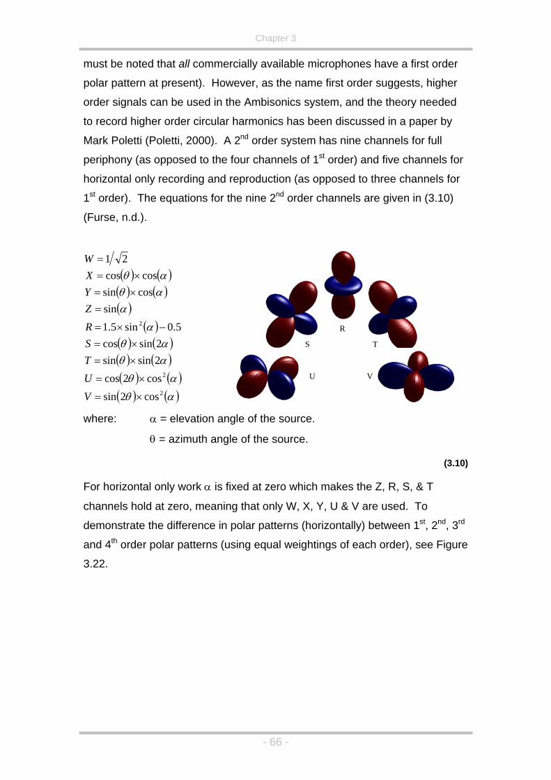
Chapter 3
must be noted that all commercially available microphones have a first or
her
eded
ony (as opposed to the four channels of 1st order) and five channels for
horizontal only recording and reproduction (as opposed to three channels for
1st order). The equations for the nine 2nd order channels are given in (3.10)
(Furse, n.d.).
der
polar pattern at present). However, as the name first order suggests, hig
order signals can be used in the Ambisonics system, and the theory ne
to record higher order circular harmonics has been discussed in a paper by
Mark Poletti (Poletti, 2000). A 2nd order system has nine channels for full
periph
( ) ( )( ) ( )( )
( )( ) ( )( ) ( )( ) ( )( ) ( )αθ
αθ
αθαθ
α
ααθαθ
2
2
2
cos2sincos2cos
2sinsin2sincos
5.0sin5.1sin
cossincoscos
21
×=
×=
×=×=
−×=
=×=×=
=
VUTSRZYXW
where: α = elevation angle of the source.
)
For horizonta zero which makes the Z, R, S, & T
, 3
V
R
T S
U
θ = azimuth angle of the source.
(3.10
l only work α is fixed at
channels hold at zero, meaning that only W, X, Y, U & V are used. To
demonstrate the difference in polar patterns (horizontally) between 1st, 2nd rd
and 4th order polar patterns (using equal weightings of each order), see Figure
3.22.
- 66 -

Chapter 3
Figure 3.22 Four different decodes of a point source polar patterns of 1st, 2nd, 3rd &
4th order systems (using virtual cardioid pattern as a 1st order reference and equal weightings of each order). Calculated using formula based on equation (3.4), using an azimuth of 1800 and an elevation of 00 and a directivity factor (d) of 1.
ers
are working at the same time; they are just working in a different way to
reconstruct the original sound field. Figure 3.23 shows the decoded levels for
rce is
.
r each
f
Higher order polar patterns, when decoded, do not imply that fewer speak
an infinite number of speakers placed on the unit circle. The virtual sou
placed at 1800 and the virtual decoder polar pattern is set to that shown in
Figure 3.22. The multiple lobes can clearly be seen at 1800 for the second
order decode and at approximately 1300 and 2500 for the third order decode
Note that the peak at the source position is not necessarily the same fo
Ambisonic order (the responses were scaled in Figure 3.22, but this is a
decoder issue), but the sum of all the decoder feeds (divided by the number o
speakers) is equal to 1 for each order. This means that the measured
pressure value at the middle of the speaker array will be consistent.
- 67 -

Chapter 3
Figure 3.23 An infinite speaker decoding of a 1st, 2nd, 3rd & 4th order Ambisonic
source at 1800. The decoder’s virtual microphone pattern for each oris shown in Figure
der 3.22.
Figure 3.23. For
xample, if we take a 1st and a 2nd order signal and reproduce this over four
rs to be
rs is
One point not mentioned so far is that there are a minimum number of
speakers needed to successfully reproduce each Ambisonic order, which is
always greater than the number of transmission channels available for the
decoder (Gerzon, 1985). This problem can be compared with the aliasing
problem in digital audio, that is, enough ‘samples’ must be used in the
reproduction array in order to reproduce the curves shown in
e
speakers (knowing that a 2nd order signal will need at least six speake
reproduced correctly) then the amplitude of the signals at the four speake
shown in Figure 3.24. It can clearly be seen that speakers two and four (at
900 and 2700 respectively) have no output, whereas speaker 3 (positioned at
1800) has an amplitude of 1, coupled with the opposite speaker (at 00) having
an output amplitude of 1/3.
- 68 -

Chapter 3
st ndFigure 3.24 Graph of the speaker outputs for a 1 and 2 order signal, using four speakers (last point is a repeat of the first, i.e. 00/3600) and a source position of 1800.
This will result in the image pulling towards one speaker when the source
position is ne
985) and w e the decoding to favour the directions at the speaker
locations. This is detrimental to the reproduced sound field as one of the
resounding features of Ambisonics is that all directions are given a constant
error, making the speakers ‘disappear’, which is one reason as to why
Ambisonics can give such a natural sounding reproduction.
Recent work by Craven (2003) has now described a panning law (as
described in the paper, which is analogous to an Ambisonic decoder) for
irregular speaker arrays using 4th order circular harmonics. This uses the
velocity and energy vector theories mentioned above to optimise the decoder
for the ITU irregular 5-speaker array. What is interesting about this decoder is
that although 4th order circular harmonics are used, the polar patterns used for
the virtual microphone signals are not strictly 4th order (as shown in Figure
3.22) but are , 3 and 4 order components in order to
teer the virtual microphone polar patterns so that the performance of the
ar that direction. This is also shown in the research by Gerzon
ill caus(1
‘contaminated’ with 2nd rd th
s
- 69 -

Chapter 3
decoder is maximised (which means having a high order front and low order
rear decode, dependant on speaker density). The velocity and energy vec
analysis of the 4
tor
th order decoder used by Craven (2003) can be found in
Figure 3.25 and the corresponding virtual microphone patterns can be seen in
Figure 3.26.
Figure 3.25 Energy and Velocity Vector Analysis of a 4th Order Ambisonic decoder
for use with the ITU irregular speaker array, as proposed by Craven (2003).
Figure 3.26 Virtual microphone patterns used for the irregular Ambisonic decoder
as shown in Figure 3.25.
- 70 -

Chapter 3
It must also be noted that a number of researchers have now started to work
on much higher orders of Ambisonics (for example, 18th order) and it is at
Ambisonics does, indeed, tend towards a system similar to
003)
,
w and high frequencies. This makes it an ideal
choice for a system that can be converted to binaural and transaural
re apparent:
•
the e of
and .
• ers are
added (Gerzon & Barton, 1992 and Gerzon & Barton, 1998).
e actual
and
these orders that
wavefield synthesis (see Sontacchi & Holdrich, 2003 and Daniel et al., 2
and although these, much higher order systems, will not be utilised in this
report, the underlying principles remain the same.
3.3.1.5 Summary
Ambisonics is an ideal system to work with for a number of reasons:
• It has both a well defined storage format and simple synthesis equations
making it useful for both recording/mixing and real-time synthesis.
• The encoding is separated from the decoding resulting in a system where
decoders can be designed for different speaker arrays.
• The design of a decoder is based on approximations to what a centrally
seated listener will receive, in terms of phase and level differences
between the ears at lo
reproduction.
However, a number of issues a
The optimisation of a frequency dependant 1st order decoder for use with
ITU 5 speaker array has not been achieved with the techniqu
solving the non-linear simultaneous equations representing the velocity
energy vectors being both laborious and leading to non-ideal results
This process will only become more complicated when more speak
• The energy and velocity vectors are low order approximations to th
head related signals arriving at the ear of the listener. The analysis
design of Ambisonic decoders could, potentially, be improved through the
use of head related data directly.
- 71 -
Chapter 3
3.3.2 Wavefield Synthesis
3.3.2.1 Theory
Although this research concentrates on the Ambisonic form of speaker
surround sound, it is not necessarily because it is the most realistic in its
listening experience. One of the most accurate forms of surround sound
(from a multiple listener point-of-view) is termed Wavefield Synthesis. In its
simplest form Wavefield Synthesis is the system first tried by Bell Labs
mentioned at the beginning of this chapter (Rumsey and McCormick, 1994);
however, the theory and underlying principles of Wavefield Synthesis have
been studied, the mathematical transfer functions calculated and a theoreti
understanding of the necessary signal processing involved in such a system
have been developed. The result is that individual sources can be
synthesised, simulating both angular placement and distance (with distance
being the cue that is, perhaps, hardest to recreate using other multi-speaker
reproduction systems).
Wavefield synthesis is different from most other multi-speaker surround
systems in a num
cal
sound
ber of ways:
• It is a volume solution, that is, there is no ‘sweet spot’, with an equal
avefield Synthesis (and the Bell Labs version before it) is based on
Huygen’s princi 1 ny wave front can be
recreated by using any number of point sources that lie on the original wave.
This implies that to recreate a plane wave (i.e. a source at an infinite dista
but to create a
reproduction quality experienced over a wide listening area.
• Distance simulation is very well suited to Wavefield Synthesis. This is
a difficult cue to simulate using other forms of multi-channel sound.
• The resulting acoustic waves, rather than the source itself, are
synthesised.
W
ple . Put simply this states that a
nce
from the listener) a line-array of speakers must be used,
1 The principle that any point on a wave front of light may be regarded as the source of
econdary waves and th he s ves can be used to
determine the future position of the wave front.
s at t urface that is tangent to the secondary wa
- 72 -

Chapter 3
spherical wave (more like the waves heard in real life) an arc of speakers
ly
t
apsules), or necessarily needed, and so it is more accurate to
think of Ambisonics as more of an amplitude panning scheme (albeit, one
based on more solid foundations than simple pair-wise schemes). This also
suggests that the results from Bamford (1995) that state that first order
Ambisonics is only ‘correct’ up to 216Hz (in a sweet spot 25cm wide) may be
a simplification (and under-estimation) of the system’s performance. In other
words, this is a measure of an Ambisonics wavefield synthesis performance.
Clearly, if Ambisonics only had a useable (spatially speaking) frequency of up
to 216Hz, and a sweet spot 25cm wide, it would not be very useful for
surround sound.
So what is the limiting factor for Wavefield Synthesis? Due to the finite
‘Spatial Aliasing Frequency’ (Berkhout , 1992). The equation for this
must be used. However, where Wavefield Synthesis’ innovation lies is that
the necessary transfer functions have been calculated, and a line array of
speakers can synthesise both of these situations using a mixture of time
delays and amplitude scaling (a transfer function). It is often thought that
Ambisonics is spherical Wavefield Synthesis on a lesser scale, and Bamford
(1995) has analysed it in this way (that is, as a volume solution, looking at
how the well the sound waves are reconstructed); however, this is not strict
the case as no time differences are recorded (assuming perfectly coinciden
microphone c
number of points used to recreate a sound wave, this system is limited by its
t al.e
(although note that this is for a plane wave) is given in Equation (3.11)
(Verheijen et al., 1995).
( )θsin2 xcf Nyq ∆
=
(3.11)
where: fNyq = Limiting Nyquist Frequency.
∆x = Speaker spacing.
θ = Angle of radiation.
c = Speed of sound in air (≈342ms-1)
- 73 -
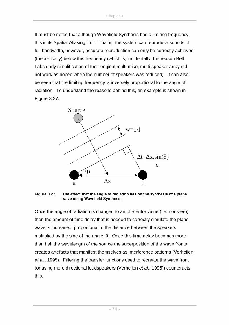
Chapter 3
It must be noted that although Wavefield Synthesis has a limiting frequency,
this is its Spatial Aliasing limit. That is, the system can reproduce sounds of
full bandwidth, however, accurate reproduction can only be correctly achieved
(the e
Labs e ray did
not wo n also
be see he angle of
rad io
Figure
has on the synthesis of a plane
wave using Wavefield Synthesis.
to an off-centre value (i.e. non-zero)
to recreate the wave front
r using more directional loudspeakers (Verheijen et al., 1995)) counteracts
this.
or tically) below this frequency (which is, incidentally, the reason Bell
arly simplification of their original multi-mike, multi-speaker ar
rk as hoped when the number of speakers was reduced). It ca
n that the limiting frequency is inversely proportional to t
iat n. To understand the reasons behind this, an example is shown in
3.27.
Figure 3.27 The effect that the angle of radiation
Once the angle of radiation is changed
then the amount of time delay that is needed to correctly simulate the plane
wave is increased, proportional to the distance between the speakers
multiplied by the sine of the angle, θ. Once this time delay becomes more
than half the wavelength of the source the superposition of the wave fronts
creates artefacts that manifest themselves as interference patterns (Verheijen
et al., 1995). Filtering the transfer functions used
(o
a b∆x
∆t=∆x.sin( θ )
θ
Source
w=1/f
c
- 74 -

Chapter 3
3.3.2.2 Summary
Wavefield Synthesis is reported as being one of the most accurate forms of
multi-channel sound available, but it does have some problems that make it
an undesirable solution for this project:
• Huge amount of transducers needed to recreate horizontal surround
sound (for example, the University of Erlangen-Nuremberg’s
experimental setup uses 24 speakers (University of Erlangen-
Nuremberg, N.D) arranged as three sides of a square).
• The reproduction of three-dimensional sound is not yet possible using
Wavefield Synthesis.
ield Synthesis is
difficult due to the high rejection needed for each direction.
for
e
g techniques. An example of the two dimensional
algorithm is shown in Figure 3.28 (Pulkki, 1997).
• Recording a sound field for reproduction using Wavef
Synthesised material works much better (Verheijen et al., 1995).
• Large amount of storage channels and processing power needed to
provide loudspeakers with appropriate signals.
Also, there is not, as yet, a standard protocol for the storage and distribution
of such material; although this is being worked on as part of the MPEG
Carusso Project (Ircam, 2002). This lack of storage standard is not an issue,
of course, for applications that calculate their acoustical source information on
the fly, such as virtual reality systems.
3.3.3 Vector Based Amplitude Panning
3.3.3.1 Theory
Vector based amplitude panning (or V.B.A.P.) is an amplitude panning law
two or three dimensional speaker rigs, and was developed by Ville Pulkki.
Once the speaker positions are known, the V.B.A.P. algorithm can then be
used to decode the speaker rig using pair-wise (two dimensions) or triple-wis
(three dimensions) pannin
- 75 -

Chapter 3
g2l2g 1 l 1
Source
Figure 3.28 Graphical representation of the V.B.A.P. algorithm.
to its
two compone , which are then
r the amount of the source that it supplied to each of the
ting
g2.
the
r
he same direction as
speaker as only that speaker will be replaying sound. This will create a
l source (as it is now a real
sou
the speakers it too great.
As can be seen in Figure 3.28, horizontal V.B.A.P. divides the source in
nt gains, in the direction of the loudspeakers
used as the gains fo
speakers. It must be noted, however, that the sources are limited to exis
on the path between speakers by normalising the gain coefficients g1 and
To extend the system to three dimensions, triple-wise panning is used. An
example decode of a source travelling from an angle of 00 to an angle of 1200
is shown in Figure 3.29, along with the four un-normalised speaker gains.
This system can work very well, mainly because the largest possible
localisation error cannot be any more than one speaker away from where
source should be. However, as can be observed from Figure 3.29, a speake
detent effect will be noticed when a source position is in t
a
more stable, and psychoacoustically correct virtua
source) which will mean that the individual speakers will be heard with the
rces potentially jumping from speaker to speaker if the spacing between
- 76 -

Chapter 3
Speaker Amplitude Source at 00 Source at 300
Sou eFigure
s
are
ill
ion is calculated when
the material is replayed, as information regarding the speaker layout must
be known.
• The decoded material is not optimis
making the system sub-opt
systems is required.
rc at 600 Source at 900 Source at 1200
3.29 Simulation of a V.B.A.P. decode. Red squares – speakers, Blue pentagram – Source, Red lines – speaker gains.
3.3.3.2 Summary
VBAP is based around the simple pair-wise panning of standard stereo,
although using the VBAP technique it can be easily used as a triple-wise,
with-height system. To this end, a VBAP system comprising of a low number
of speakers will suffer the same problems as other pair-wise panned system
(see Quadraphonics, section 3.2.7). However, as the number of speakers
increased, the accuracy of the system will improve, although side images w
always suffer when compared to frontal images due to pair-wise panning
techniques failing for speakers placed to the side of a listener (although the
error will, again, lessen with increased speaker density).
For this project, however, VBAP is unsuitable as:
• VBAP has no storage format – all panning informat
• Any pre-decoded material can not have additional speaker feeds
calculated according to the rules of VBAP.
ed for a centrally seated listener,
imal if conversion to headphone or transaural
- 77 -
Chapter 3
3.3.4 Two Channel, Binaural, Surround Sound
Although all of the surround sound systems discussed so far have used more
than two channels (many more, in some cases), it is possible to use only two
channels. Such a system is termed binaural reproduction. As we only have
two ears, then it seems reasonable that only two channels of audio are
necessary to successfully fool the ear/brain system into thinking that it is
experiencing a realistic, immersive, three dimensional sound experience. All
of the speaker reproduction systems discussed so far have a number of
marked limita
• System performance is normally proportional to the number of
ore
r.
•
Binaur of headphones. As
the i
provide und
sound.
ars are supplied with the same acoustical pressure that would have been
uses
e a sound source, a number of which can be simulated using a head
lated transfer function (HRTF). An example pair of HRTFs are shown in
tions:
speakers used. The more speakers, the better the result.
• The sound from each speaker will reach both ears, making it a m
involved task to control exactly what is being perceived by the listene
The final system is usually a compromise due to the above limitations.
al sound circumvents these limitations with the use
re s a one to one mapping of the ears to the transducers it is very easy to
the ears with the signals necessary to provide convincing surro
Binaural sound reproduction works on the simple principle that if the
e
present in real-life due to a real source, then the ear/brain system will be
fooled into perceiving that a real source is actually there. As discussed in
chapter 2, there are a number of auditory cues that the ear/brain system
to localis
re
Figure 3.30, and are taken from a KEMAR dummy head in an anechoic
chamber by Gardner & Martin (1994). The source was at an angle of 450
from the centre of the head, and at a distance of 1 m.
- 78 -

Chapter 3
Figure 3.30 Pair of HRTFs taken from a KEMAR dummy head from an angle of 450 to
the left and a distance of 1 metre from the centre of the head. Green – Left Ear, Blue – Right Ear.
The three lateralisation cues can be clearly seen in this figure. These are:
• Amplitude differences – amplitude is highest at the nearer ear.
• Time differences – farther ear signal being delayed compared to the
closer ear (seen in both the time domain plot, and the phase response
plot, by observing the larger [negative] gradient).
• Pinna and head filtering – as the s
ound has two different physical paths
to travel to the ears, due to the pinna and the head, resulting in
ophones into the ear of the recordist (or
dummy head). The parts of the outer ear that filter the incoming sound wave
are the pinna and the ear canal. If the recorded material is taken from a
subject with an open ear canal (i.e. microphones placed in the ear of the
subject) then the recording will possess the ear canal resonance, which lies at
about 3 kHz (a 3 cm closed pipe has a fundamental resonant frequency of
frequency dependent filtering (seen in the frequency response plot).
It is the head related transfer function that forms the basis on which binaural
sound reproduction is founded, although through the use of anechoic HRTF
data alone, only simple lateralisation is possible. This will be discussed
shortly.
There are two ways in which to create a binaural reproduction, it can be
recorded using in-ear microphones, or it can be synthesised using HRTF
data. As far as the recording side of binaural sound is concerned, the theory
is as simple as placing a pair of micr
- 79 -
Chapter 3
2850 Hz). Then, when the listener replays the recording over headphones,
the recording will be subjected to another ear canal resonance, meaning that
the musical content will be perceived as having a large resonance at around 3
kHz. This, therefore, must be corrected with the use of equalisation; although
the blocking of the ear canal of the recordist prior to recording is another
solution (Kleiner, 1978). The actual positioning of the microphones within the
outer ear of the subject has an effect on the system where the most robust
positioning of the microphone is usually found to be inside the ear canal
(Ryan & Furlong, 1995), (although the blocking of the ear canal is not really a
desirable solution to the last problem). There are two other difficulties in
using recorded binaural material and they are pinna individualism and head
movements. As discussed in Chapter 2, everyone’s pinnae are different,
n ns that the pinnae apply to
. As
n it will
ble to
which in tur means that the complex filtering patter
the incoming sound waves are also different. The binaural recording process
means that the listener will be experiencing the sound field by listening
through somebody else’s ears. The results of this will be discussed later in
this section.
When it comes to synthesising a binaural sound field, HRTF data is used
the HRTF is a measure of the response of the ear due to a source, the
suffer the same difficulties mentioned for the recorded material. However,
some differences are apparent. The HRTF data used to synthesise sources
is normally recorded in an anechoic chamber (Gardner and Martin, 1994) as
this gives the greatest flexibility in source position synthesis as it is possi
add reverberation, but very difficult to take it away again. Also, HRTFs are
usually recorded in pairs at a set distance from the centre of the head (say,
one metre), but this is not necessarily the most versatile solution. As a
demonstration of this, consider the situation shown in Figure 3.31.
- 80 -

Chapter 3
Source
Listeners Ears
1 Metre
HRTF Directions from
1 metre
3.31 Example of a binaural synthesis problem. Figure
If distance is to be simulated correctly, then recording and storing the HRTFs
in p rs
becaus difference,
e
s
the
irable
ural
just resulting in source lateralisation) is not usually possible using anechoic
ai centred on the head actually complicates the situation. This is
e the pair of HRTFs will have an amplitude difference, time
and pinna filtering that is not only due to the angle of incidence of the source,
but also its distance, as discussed in Chapter 2. This means that if a sourc
is to be synthesised at a distance that is different than the one that wa
measured then the point at which the source intersects the measured
distance needs to be obtained. Extra delay also needs to be added to
HRTF filters, with a different value added to the left and right HRTFs. This
adds extra, avoidable, calculations to the synthesis model, and is undes
in real-time applications. To combat this problem it is far better that the
HRTFs be recorded taking each ear as the centre point for the measurements
as this means that the angle from source to each of the listener’s ears needs
to be calculated, which is simpler than the scheme detailed above (although
extra delay does still need to be added for each response separately).
Once the problem of angle of incidence has been resolved (with one of the
two methods suggested above) then one of the main advantages of bina
theory can come into play, and that is the simulation of distance cues.
However, obtaining sources that are localisable outside of the head (i.e. not
- 81 -
Chapter 3
simulation of the source (McKeag & McGrath, 1997). This, in some respects
is to be expected, as one of the psycholog
,
ical effects of being in an anechoic
hamber is that sources tend to be perceived much closer than they actually
f source
ation
r/brain system uses small head
rotations to resolve the position of a source within the cone of
e
aural sound, while
er, it can be seen that
eag
rding
, and
erience
c
are. One of the mechanisms that the brain utilises in the perception o
distance is in the direct to reverberant ratio of sounds (see Chapter 2).
Sounds that are very close to the head have a very low (if any) reverber
perceived with them, so if a sound is heard in an anechoic chamber then the
brain may assume that this source is close to us because of this. However,
when listening to synthesised binaural sources it is unlikely that true, or even
any, distance information will be perceived. This is due, mainly, to the
reasons given below:
• In nearly all listening situations the ea
confusion.
• The shape and, therefore, filtering of the sound due to the pinna of th
recording subject will be different than that of the listener.
A number of people (including Moller et al., 1996) suggest that individualised
HRTFs are needed for the accurate reproduction of bin
others suggest that head tracking is the most important aspect of the
localisation process (Inanaga et al., 1995). Howev
neither or these are necessarily needed, and depth perception can be
achieved by creating multiple, coherent auditory cues for the listener (McK
& McGrath, 1997). Again, depending on the application, there are two
methods of achieving this. Firstly, for the simulation of sources that are in a
fixed position, the HRTFs can be measured in a real room, thereby reco
the room’s actual response to a source, in this position, at the two ears of a
subject. This, when convolved with the source material, will create the illusion
of a source outside the head of the listener (McKeag & McGrath, 1997).
Secondly, if dynamic source movement is needed, such as in 3D gaming
virtual reality applications, then a model of the room in which the source is
placed must be realised separately from the source, and then all of the
images synthesised using anechoic HRTF data. The binaural synthesis of
material in this way can lead to a very convincing surround sound exp
- 82 -
Chapter 3
using a limited number of channels, which is probably why all 3D computer
gaming cards use this form of modelling.
As mentioned in Chapter 1, it is now widely recognised that binaural
headphone reproduction techniques can be used as a method of auralising
multi-speaker arrays. This technique was pioneered by Lake DSP (for
example, see McKeag & McGrath (1997) and McKeag & McGrath (1996) as
an example of their later work), and more recently has been used by others
(for example, see Leitner et al., 2000 and Noisternig et al, 2003) as a method
of simulating both discrete speaker feeds and, in the case of Ambisonics,
realising an Ambisonic decoder efficiently as three or four HRTF filters (see
y
d
fact
is
hat
r at
one ear of the listener? This situation is shown in Figure 3.32, but is
simplified by taking each ear as a microphone in a free field (i.e. no filtering of
Chapters 4 and 5 for more details on this).
Interestingly, although three of the four papers mentioned above discuss
Ambisonics to binaural conversion, none use psychoacoustically optimised
decoders as discussed in section 3.3.1.2. This will result in sub-optimal
lateralisation parameters being reproduced at the listeners ears, as shown in
the non-optimised decoders discussed in section 5.2.
3.3.5 Transaural Surround Sound
Transaural surround sound techniques were first proposed in the 1960’s b
Atal, Hill and Schroeder (Atal, 1966) and, although based on a relatively
simple and understandable principle, were difficult to realise at this time.
Transaural sound is a process by which Binaural reproduction can be realise
over loudspeakers. Loudspeaker reproduction differs from headphone
reproduction in that the sound from one loudspeaker reaches both ears (a
that is the basis of Blumlein’s stereo reproduction technique, see earlier in th
chapter), and binaural reproduction over headphones relies on the fact t
the signal from one transducer only reaches one ear, that is, there is no
crosstalk between the ears of the listener. The Transaural system is easier to
explain if the following problem is considered. If a pulse is emitted from one
of a pair of loudspeakers, what must happen for that pulse to only appea
- 83 -

Chapter 3
the sound will be present due to the head of the listener). Each of the two
speakers are equidistant from the centre of the two microphones, and subtend
an angle of 60 degrees (+/- 300).
M ic 2 M ic 1 Figure 3.32 Graphical representation of the crosstalk cancellation problem.
It can be noted that Mic1 receives the pulse first, closely followed by Mic2
which receives the same pulse, except that the amplitude has attenuated and
it arrives later in time due to the extra distance travelled. In order to cancel
o that the same amplitude as the signal arriving at Mic2 is achieved, but
inverted (1800 out of phase) as shown in Figure 3.33. This signal now
cancels out the first sound pi
to each speaker’s output in Figure 3.
another signal, again amp
reduced and phase inverted,
counteract the Mic1 crosstalk signal,
pulses is always diminishing, a realisable
Figure 3.34. Also shown in Figure 3.34 is the block diagram for a typical
tio ill
rosstalk can
the sound arriving at Mic2, the left loudspeaker can be made to emit a sound
s
cked up by Mic2 (see the microhpones response
33), but then the crosstalk produces
litude reduced, at Mic1. So another, amplitude
signal is produced from the right loudspeaker to
and so on. As the amplitude of these
and stable filter results, as shown in
implementa n of a crosstalk cancellation system, note that this system w
cel for both speakers, that is, the Left input signal will only c
appear at Mic2 and the Right input signal will only appear at Mic1. These two
filters can be realised using a pair of I.I.R. filters1. However, this structure is
not used, in practice, as the response of the listener’s head is not taken into
account and so this form of crosstalk cancellation will be sub-optimal.
1 Infinite Impulse Response filters using a feedforward/back loop and attenuating gain factors
(typically).
- 84 -

Chapter 3
Figure 3.33 Simulation of Figure 3.32 using the left loudspeaker to cancel the first
sound arriving at Mic2.
0 50 100 150 200 250 300 350 400 4500
0.2
0.4
0.6
0.8
1A graph showing Two Free Field Dipole Filters
Am
plitu
de
Time (samples)
0 50 100 150 200 250 300 350 400 450-1
-0.8
-0.6
-0.4
-0.2
0
Time (samples)
Am
plitu
de
0 50 100 150 200 250 300 350 400 4500
0.2
0.4
0.6
0.8
1
0 50 100 150 200 250 300 350 400 4500
0.2
0.4
0.6
0.8
1A graph showing Two Free Field Dipole Filters
Am
plitu
de
A graph showing Two Free Field Dipole Filters
Am
plitu
de
Time (samples)
0 50 100 150 200 250 300 350 400 450-1
-0.8
-0.6
-0.4
-0.2
0
Time (samples)
0 50 100 150 200 250 300 350 400 450-1
-0.8
-0.6
-0.4
-0.2
0
Time (samples)
Am
plitu
de
Figure 3.34 Example of free-field crosstalk cancellation filters and an example
implementation block diagram.
Although this particular filtering model would never be used in practice, it will
be used here to demonstrate the type of frequency response changes that
occur due to the crosstalk cancellation filtering process. In theory, of course,
sweet spot in a
on-anechoic room) will have a response similar to that shown in Figure 3.35.
Left
Right
H2
H1Left
Speaker
Right Speaker
the sounds heard at the two microphone positions will be as desired, but for
off centre listening (and also, to some extent, listening in the
n
- 85 -

Chapter 3
Although this seems slightly irrelevant for crosstalk cancellation filters
designed with HRTF data, it does show so ng that can
occur due to the system inversion process.
me of the extreme filteri
Figure 3.35 Frequency response of free field crosstalk cancellation filters
The process above, described as filter inversion is, in fact, slightly more
complicated than this. Although the example above (crosstalk cancellation in
the free field) is a good starting point for gaining an understanding of the
processes involved in crosstalk cancellation algorithms, the equation has not
yet been defined. If we again look at the problem shown in Figure 3.36, it
can be seen that, for a symmetrical setup, only two transfer functions are
nd c2 –
the response
present, c1 – the response of the microphone to the near speaker, a
of the microphone to the far speaker.
M ic2 M ic1
c1 c1c2c2
v2 v1
Figure 3.36 The Crosstalk cancellation problem, with responses shown.
The relationship between the signals emanating from the speakers, and what
arrives at the two microphones is given in Equation (3.12).
- 86 -

Chapter 3
⎥⎦
⎤⎢⎣
⎡⋅⎥⎦
⎤⎢⎣
⎡=⎥
⎦
⎤⎢⎣
⎡
2
1
12
21
21
vv
cccc
MicMic
(3.12)
needs to be applied to the two signals, prior to transmission (Nelson et al
ll be
Therefore, if we wish to present to the system the signals that we wish to
receive at Mic1 and Mic2, then the inverse of the transfer function matrix
.,
1997) (which is what is happening in the system described in Figure 3.34) and
is shown in Equation (3.13). The simplification to two filters, h1 and h2 can be
made due to the crosstalk cancellation meaning that the signal at Mic2 wi
forced to zero and the signal at Mic1 will be the desired signal at unity gain.
( ) ( ) ⎥⎦
⎤⎢⎣
⎡⋅⎥
⎦
⎤⎢⎣
⎡−
−×−×
=⎥⎦
⎤⎢⎣
⎡211
12
21
22112
1
MicMic
cccc
ccccvv
12
21
22
21
22
22
1
12
22
21
22
22
1
11
ccc
cv −−
=
⇒
22
21
22
22
21
11
ccch
ccc
Miccc
cMiccc
c
Miccc
Mic
⋅−−
+⋅−
=
⋅−
+⋅
v
h
−−
=
−=
(3.13)
where: v1 & v2 are the speaker signals shown in Figure 3.36
c1 & c2 are the transfer functions from Figure 3.36.
h1 & h2 are the transfer functions used in Figure 3.34.
The final filters are shown in Equation (3.14) (the multiplying of c12
+ c22 to
compatibility edure) and is carried
both the numerator and denominator of the equation is also shown for
with the frequency dependent inversion proc
out in the frequency domain, adapted from Farina, et al. (2001), as inverting
this system in the time domain can take a long time, even on fast computers.
As an example, the calculation of the these filters in the frequency domain,
using Matlab® and a filter size of 1024 points takes less than a second,
however, using time domain signals coupled with the simple multiplications
and divisions turning into convolutions and de-convolutions means that the
same algorithm can take around half an hour to complete.
- 87 -

Chapter 3
⎟⎠
⎜⎝ − 4
241
11 cc⎟⎞
⎜⎛ +
×=22
21 ccch ⎟
⎠⎜⎝ − 4
241
22 cc
where: c1 & c2 are the transfer functions from Figure 3.36.
h1 & h2 are the transfer functions used in Figure 3.34.
(3.14)
It must also be noted that Equation (3.14) shows the inversion procedure for
identical), an
mathematical equation has been defined, any transfer function can be used
⎟⎞
⎜⎛ +
×−=22
21 ccch
the symmetrical case (that is, the diagonals of the transfer function matrix are
d is not the general solution for this problem. Now that the
for c1 and c2 and a non-free field situation simulated. For example, if two
speakers were spaced at +/- 300, as in a normal stereo triangle, then the
corresponding crosstalk cancellation filters will be the same as shown in
Figure 3.37.
Figure 3.37 Transfe
their corrr functions c1 and c2 for a speaker pair placed at +/- 300, and
esponding crosstalk cancelling filters.
As can be seen in the right hand graph of Figure 3.37, the crosstalk
cancellation filters actually have samples that are valued greater than one
(which denotes potential clipping in many audio applications); however, in this
amplification w
cancellation f .
case, they will not clip themselves (so long as storing these filters is not a
problem). Nevertheless, when they are applied to a signal, much
ill arise. The frequency responses of the two crosstalk
ilters are given in Figure 3.38
- 88 -
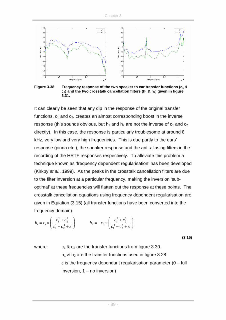
Chapter 3
Figure 3.38 Frequency response of the two speaker to ear transfer functions (c1 &
c2) and the two crosstalk cancellation filters (h1 & h2) given in figure 3.31.
It can clearly be seen that any dip in the response of the original transfer
functions, c1 and c2, creates an almost corresponding boost in the inverse
response (this sounds obvious, but h1 and h2 are not the inverse of c1 and c2
ow
n the
e
points. The
crosstalk cancellation equations using frequency dependent regularisation are
given in Equation (3.15) (all transfer functions have been converted into the
frequency domain).
directly). In this case, the response is particularly troublesome at around 8
and very high frequencies. This is due partly to the ears’ kHz, very l
response (pinna etc.), the speaker response and the anti-aliasing filters i
recording of the HRTF responses respectively. To alleviate this problem a
technique known as ‘frequency dependent regularisation’ has been developed
(Kirkby et al., 1999). As the peaks in the crosstalk cancellation filters are du
to the filter inversion at a particular frequency, making the inversion ‘sub-
optimal’ at these frequencies will flatten out the response at these
⎟⎟⎠
⎞⎜⎜⎝
⎛+−
+×=
ε42
41
22
21
11 ccccch ⎟⎟
⎠
⎞⎜⎜⎝
⎛+−
+×−=
ε42
41
22
21
22 ccccch
(3.15)
where: c1 & c2 are the transfer functions from figure 3.30.
h1 & h2 are the transfer functions used in figure 3.28.
ε is the frequency dependant regularisation parameter (0 – full
inversion, 1 – no inversion)
- 89 -
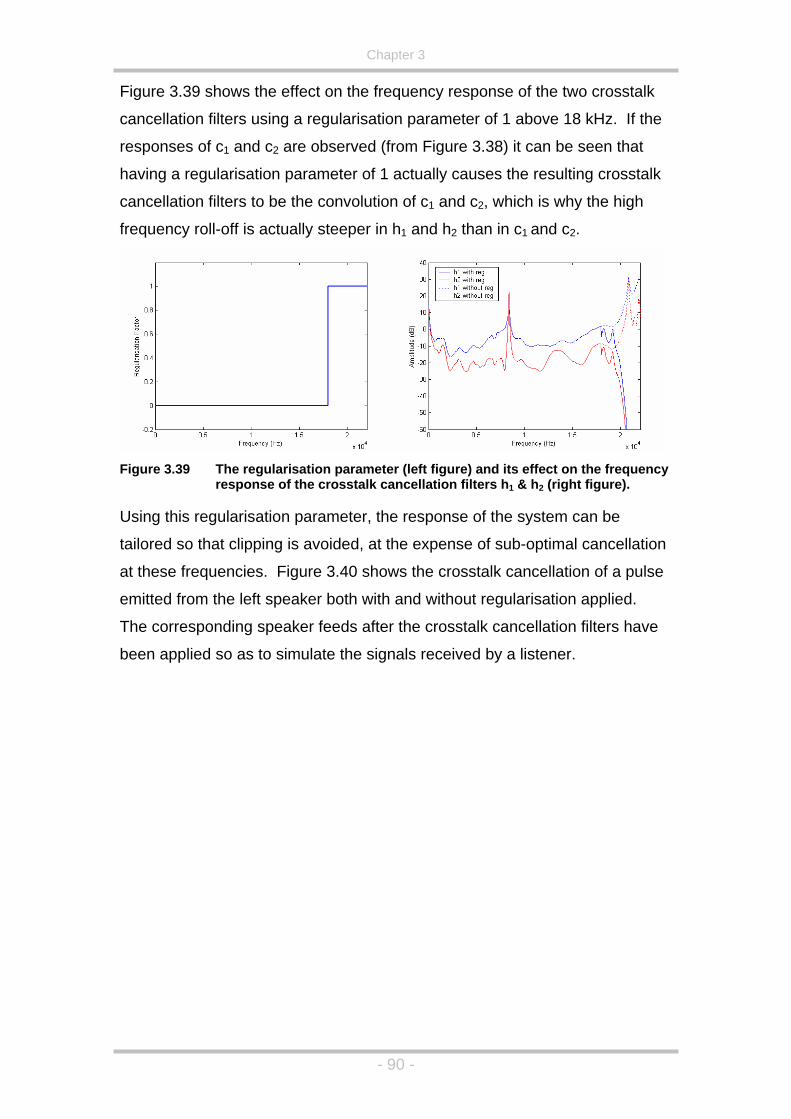
Chapter 3
Figure 3.39 shows the effect onse of the two crosstalk
cancellation filters using a regularisation parameter of 1 above 18 kHz. If the
responses of c1 and c2 are observed (from Figure 3.38) it can be seen that
having a regularisation parameter of 1 actually causes the resulting crosstalk
cancellation filters to be the convolution of c1 and c2, which is why the high
frequency roll-off is actually steeper in h1 and h2 than in c1 and c2.
on the frequency resp
Figure 3.39 The regularisation parameter (left figure) and its effect on the frequency
response of the crosstalk cancellation filters h1 & h2 (right figure). Using this regularisation parameter, the response of the system can be
tailored so that clipping is avoided, at the expense of sub-optimal cancellation
at these frequencies. Figure 3.40 shows the crosstalk cancellation of a pulse
emitted from the left speaker both with and without regularisation applied.
The corresponding speaker feeds after the crosstalk cancellation filters have
been applied so as to simulate the signals received by a listener.
- 90 -

Chapter 3
With Regularisation
Without Regularisation
Figure 3.40 Simulation of crosstalk cancellation using a unit pulse from the left
channel both with and without frequency dependent regularisation applied (as in Figure 3.39).
Assuming that any value greater than one will cause clipping of the signal
then it can be clearly seen that when regularisation is applied to the crosst
cancellation
alk
filters the system outputs much lower signals while still
aintaining almost the same signal level at the ears of the listener (it must be
noted that in this simulation the same HRTF data was used for both the
m
- 91 -

Chapter 3
simulation and the calculation of the crosstalk cancellation filters, and this will
not be true in a real-life situation).
Apart from the frequency dependent regularisation parameter introduced
above, much of the theory behind Transaural sound reproduction has not
changed since its invention in 1962 (Atal, 1966). However, spacing the
speakers as a standard stereo pair meant that the sweet spot (the area where
crosstalk cancellation occurs) is small and very susceptible to errors due to
head movement. To combat this, researchers at Southampton University
discovered that this problem, and to a certain extent, that of excessive signal
colouration, could be alleviated by moving the speakers closer together to
span around 100. If a small speaker span is used then the area of successful
crosstalk cancellation becomes larger as a line of crosstalk cancellation is
created. This means that the position of the listener with respect to the
distance from the loudspeakers is not so important, making the system more
robust. Also, to demonstrate the signal colouration changes we will again
consider the system shown in Figure 3.36. As the angular separation of the
speakers becomes smaller, the more identical the transfer functions between
each ear and the speakers (particularly at low frequencies) and hence, the
greater the amplitude of the cancellation filters at these frequencies. This
means that the angular separation of the speakers is limited by the amount of
boost that must be applied to the low frequencies of the system (assuming
regularisation is not used). An example of filters taking into account the HRTF
wings and r hen dealing with the
system. Moving the speakers closer
together makes for a more robust system, and moves much of the sound
colouration into a higher frequency range, but creates a wider range of bass
boost, which speakers generally find more difficult to recreate. Optimisation
of this technique to alleviate some of these problems will be discussed in
Chapter 5.
of the listener is shown in Figure 3.42. This, to some extent, shows the
oundabouts’ situation that can occur w‘s
speaker placement of a Transaural
- 92 -

Chapter 3
Figure 3.41 Example of the effect of changing the angular separation of a pair of
speakers used for crosstalk cancellation.
- 93 -
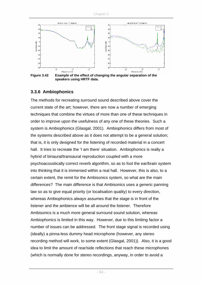
Chapter 3
chniques that combine the virtues of more than one of these techniques in
rder to improve upon the usefulness of any one of these theories. Such a
system is Ambiophonics (Glasgal, 2001). Ambiophonics differs from most of
the systems described above as it does not attempt to be a general solution;
that is, it is only designed for the listening of recorded material in a concert
hall. It tries to recreate the ‘I am there’ situation. Ambiophonics is really a
hybrid of binaural/transaural reproduction coupled with a more
psychoacoustically correct reverb algorithm, so as to fool the ear/brain system
into thinking that it is immersed within a real hall. However, this is also, to a
certain extent, the remit for the Ambisonics system, so what are the main
differences? The main difference is that Ambisonics uses a generic panning
law so as to give equal priority (or localisation quality) to every direction,
whereas Ambiophonics always assumes that the stage is in front of the
the listener. Therefore
ed using
d
Figure 3.42 Example of the effect of changing the angular separation of the speakers using HRTF data.
3.3.6 Ambiophonics
The methods for recreating surround sound described above cover the
current state of the art; however, there are now a number of emerging
te
o
listener and the ambience will be all around
Ambisonics is a much more general surround sound solution, whereas
Ambiophonics is limited in this way. However, due to this limiting factor a
number of issues can be addressed. The front stage signal is record
(ideally) a pinna-less dummy head microphone (however, any stereo
recording method will work, to some extent (Glasgal, 2001)). Also, it is a goo
idea to limit the amount of rear/side reflections that reach these microphones
(which is normally done for stereo recordings, anyway, in order to avoid a
- 94 -

Chapter 3
recording that is too reverberant (Glasgal, 2003c)). Limiting the rear and side
reflections picked up by this stereo recording is necessary due to the fact tha
these signals will be generated using convolution during the decoding stage.
This stereo signal can then be replayed using a crosstalk cancellation system
t
uch as the system described in section 3.3.5. The surrounding ambience is
the
orrect, including the pinna cues, which are
almost impossible to replicate using any other system (except Wavefield
l layout for such a system is shown in Figure 3.43.
As
means
reprod ers are
needed in front of the listener. The surround speakers are then fed with the
ste
no dire
s
then created and distributed using a number of speakers surrounding
listener. The main innovation here is that each speaker represents an early
reflection direction. This means that, as these early reflections are being
emitted from an actual source (rather than a panned position), all of the
psychoacoustic cues associated with the angular directional aspect of these
reflections will be absolutely c
Synthesis). A typica
Figure 3.43 Example Ambiophonics layout.
the crosstalk cancelled pair of speakers (typically set at +/- 50, which
multiple listeners sat in a line can experience the system) is
ucing the frontal hemisphere of the concert hall, fewer speak
reo signal convolved with a stereo pair of impulse responses which contain
ct sound, a number of discrete reflections (one or more) and a diffuse,
- 95 -
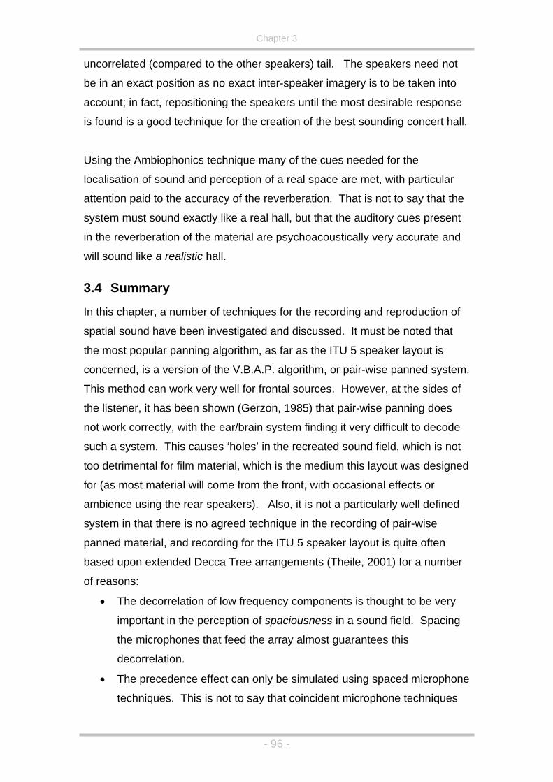
Chapter 3
uncorr t
be in a
accoun desirable response
l.
and
been investigated and discussed. It must be noted that
the o out is
concer
This m f
the list
not wo finding it very difficult to decode
suc a ot
too de igned
for (as
ambie
system
panne
based
of reas
•
g
is
• cedence effect can only be simulated using spaced microphone
techniques. This is not to say that coincident microphone techniques
elated (compared to the other speakers) tail. The speakers need no
n exact position as no exact inter-speaker imagery is to be taken into
t; in fact, repositioning the speakers until the most
is found is a good technique for the creation of the best sounding concert hal
Using the Ambiophonics technique many of the cues needed for the
localisation of sound and perception of a real space are met, with particular
attention paid to the accuracy of the reverberation. That is not to say that the
system must sound exactly like a real hall, but that the auditory cues present
in the reverberation of the material are psychoacoustically very accurate
will sound like a realistic hall.
3.4 Summary
In this chapter, a number of techniques for the recording and reproduction of
spatial sound have
m st popular panning algorithm, as far as the ITU 5 speaker lay
ned, is a version of the V.B.A.P. algorithm, or pair-wise panned system.
ethod can work very well for frontal sources. However, at the sides o
ener, it has been shown (Gerzon, 1985) that pair-wise panning does
rk correctly, with the ear/brain system
h system. This causes ‘holes’ in the recreated sound field, which is n
trimental for film material, which is the medium this layout was des
most material will come from the front, with occasional effects or
nce using the rear speakers). Also, it is not a particularly well defined
in that there is no agreed technique in the recording of pair-wise
d material, and recording for the ITU 5 speaker layout is quite often
upon extended Decca Tree arrangements (Theile, 2001) for a number
ons:
The decorrelation of low frequency components is thought to be very
important in the perception of spaciousness in a sound field. Spacin
the microphones that feed the array almost guarantees th
decorrelation.
The pre
- 96 -

Chapter 3
do not encode phase information (see Chapter 3), they just cannot
represent time of arrival differences correctly as the microphone picks
up sound from one point in space (theoretically).
However, these techniques do not lend themselves well to different speaker
arrangements (that is, they are not hierarchical based formats), and now, as
the media and technology for multi-channel sound reproduction is becoming
more readily available, the industry is starting to realise that they do not want
to rerecord/remix an album every time a new speaker layout is presented to
them. For this reason this research focuses on the Ambisonics system, which
is the only hierarchical system defined at this moment in time (although
MPEG-4 is now being specified to address this, to some extent (MIT Media
Lab, 2000)). If Ambisonics hierarchical system is used as a carrier format (in
its 1st, 2nd or higher order variants) then the system can be decoded for any
multi-speaker system. However, currently, a number of limitations are present
using this system:
• Although Gerzon and Barton (1992) suggested a number of
optimisation equations for use with irregular speaker arrangements, the
equations are difficult to solve, and so no further research seems to
have been published in this area giving optimal coefficients for use with
the standard ITU five speaker layout.
• Although a method of converting Ambisonics and five speaker ITU
surround sound to binaural reproduction has been suggested by
McKeag & McGrath (1996 & 1997 respectively), no work has been
carried out on the optimisation of these multi speaker systems in order
to reproduce the correct psychoacoustic cues at the ears of the
listener. This has been shown to be a trivial optimisation for a regular
speaker array, but will rely on the work mentioned in the point above
for the optimal auralisation of material if distributed on a medium
carrying the standard 5.1 channels as specified by the ITU standard.
• Only a handful of software utilities for the encoding and decoding of
Ambisonic material is available (McGriffy, 2002), and no
psychoacoustically correct decoding software for irregular arrays
exists.
- 97 -

Chapter 3
These current limitations will be addressed in the following chapters of this
thesis.
- 98 -

Chapter 4
Chapter 4 - Development of a Hierarchical Surround Sound Format
4.1 Introduction
Although many surround sound decoding techniques are available, a number
resentations, the
aterial is composed specifically for a particular speaker layout, and
his
ker
es obsolete, or a Binaural or Transaural production needs to be
rep e
piece he
descrip
amalg ms, in order to maximise the number
of r l
this sy
ferent speaker layouts can be used.
• The
change
pie
• The
flexible as headphones, or just a few speakers can be used. This will
cordings, or small studios, where space may be limited.
4.1.
of problems are evident. For the majority of multi-speaker p
m
Binaural/Transaural systems suffer from this same, inherent, problem. T
does not, of course, create a problem initially, but as soon as the spea
layout becom
lay d on a multi-speaker platform, a complete reworking of the sound
is needed. For these reasons, this chapter will concentrate on t
tion of a hierarchical surround sound format, based on an
amation of currently available syste
ep ay situations that the system is capable of satisfying. The benefits of
stem are:
• The created piece will be much more portable in that, as long as a
decoder is available, many dif
recordings will become more future-proof as, if a speaker layout
s, just a re-decode is needed, rather than a whole remix of the
ce.
composition/recording/monitoring of the piece will become more
result in less space being needed. This is particularly useful for on-
location re
4.2 Description of System
Such a system can be described diagrammatically as shown in Figure
- 99 -

Chapter 4
Figure 4.1 Ideal surround sound encoding/decoding scheme.
As can be seen in Figure 4.1, this ideal surround sound system should
o the
m
,
• The encoded signal should be able to be easily replayed over multiple
one
nels, each
be
n Figure 4.2.
Sound-field Manipulations. Rotations etc.
n-channel carrier
n-speaker output decoder
2-speaker trans-aural decoder
2-channel binaural decoder
Encoding Block
Recorded/ Panned Signals
conform t following criteria in order to maximise its flexibility and
usefulness:
• A hierarchical carrier signal should be used. That is, a carrier syste
should be able to be understated (channels ignored, reducing
localisation accuracy) or overstated (extra channels added later
increasing localisation accuracy).
• This encoded signal should be able to be manipulated after encoding,
i.e. rotations about the x, y and z axis etc..
listening situations including:
o A number of different speaker arrangements, as almost no-
can place their speakers in the ITU or future speaker positions.
o Over headphones.
o Over a standard stereo pair (and other placement widths) of
speakers.
• Efficient means of transferring from the carrier to one of the above
systems.
If we take the current ‘state of the art’ surround standard as an example, and
try to apply the above criteria to it, a number of shortcomings can be
observed. In Dolby Digital 5.1, the carrier signal is six discrete chan
one representing a speaker signal directly. Each speaker is assumed to
at the speaker locations specified in the ITU standard as shown i
- 100 -

Chapter 4
60
140
80 80
L RC
SL SR
Figure 4.2 Standard speaker layout as specified in the ITU standard.
To listen to this system over headphones is not a difficult task and has been
achieved by a number of companies (Mackerson et al., 1999; McKeag &
cGrath, 1997). It is achieved by binaurally simulating speakers using HRTF
ial
if a
ween 128 and 1024 samples in length. This approach
ill rely on the 5.1 decode to supply the ear/brain system with the appropriate
r,
d by Lake (McKeag & McGrath, 1997) and
tüder (Mackerson, et al., 1999)) is where the speakers are simulated in a
r
a
M
data, and replaying the resulting two channels over headphones. As
discussed in Chapter 3, the binaural reproduction of surround sound mater
needs to contain some form of psychoacoustically tangible reverb involved
realistic, out-of-head experience is to be delivered.
When auralising 5.1 surround two approaches can be taken. The first
approach assumes that the 5.1 surround system is trying to simulate an
acoustic space where each speaker can be rendered using a pair of anechoic
HRTFs, normally bet
w
reverberation, and is the most computationally efficient solution. Howeve
the qualities and amount of the reverberation used on each recording may be
psychoacoustically confusing and, therefore, not convincing enough to
promote the out-of-head imaging possible with the binaural approach. The
better approach (and the one use
S
‘good’ listening room, that is, each speaker will have its own reverb
associated with it, on top of anything that is already recorded within the
surround sound material. This can be done in one of two ways:
• Simulate the individual speakers using a pair of head related transfe
functions per speaker, and then simulate the listening room using
- 101 -

Chapter 4
binaural reverb algorithm (perhaps using discrete first order room
The decision of which of the two approaches to use is really a question of
processing power available. The difference in efficiency between the two
the second method would be used, as this would provide a closer match to a
real environment, and therefore maximising the performance of the binaural
This method has been shown to work very well, especially when carried out
with head-tracking (Makerson, et al., 1999), although a good interpolation
algorithm is then needed to stop the creation of clicks and pops due to the
changing filter structures (in fact, the development and implementation of
interpolation algorithms can be the most time consuming part of such a piece
of professional audio hardware). Once the binaural version has been created
it is then a relatively easy task to convert this recording for a 2 speaker,
transaural reproduction by using a 2 x 2 matrix of correctly designed crosstalk
cancellation filters.
d in the correct, ITU
A better technique would be to use Ambisonic B-format, or similar, to drive the
system, or at least use a standard B-format decoding algorithm to derive the 6
discrete channels on a DVD and then, if desired, work out the B-format
signals from these speaker feeds. Using a hierarchical carrier, such as B-
section.
reflections, again a pair of HRTFs per reflection, followed by a short,
diffuse tail).
• Simulate the individual speakers and room together using a much
longer pair of head related transfer functions per speaker.
methods can be quite high depending on the implementation used. Ideally
decode.
However, what if the (real) speakers were not place
specified, positions in the listening room? Calculating new speaker feeds for
a system that is defined by discrete channels is not necessarily an easy task
(Gerzon, 1992a) when the encoding system cannot necessarily be assumed
to be simple pair-wise panning.
format would result in the advantages given at the start of this
- 102 -

Chapter 4
For example, if we were to take horizontal only B-format as the carrier sig
then decoding this B-format carrier for the various different presentation
methods can be carried out as shown in Equation (4.1) (it should be noted
that this is a sub optimal decoder but this will be discussed in Chapter 5).
nal
( ) ( ) ( ) ( )ZYXWnSn ×+××+××+×= )sin()cos()sin()cos()cos(2)( φφθφθ
(4.1)
where Sn is the signal sent to the nth speaker positioned at azimuth θ and
elevation φ.
This simple decoding would produce the virtual microphone configuration
shown in Figure 4.3.
Figure 4.3 Virtual Microphone Configuration for Simple Ambisonic Decoding
4.3 B-Format to Binaural Reproduction
All multi-speaker formats can be converted to a Binaural signal, but B-Format
to binaural conversion can be achieved very efficiently due to its hierarchical
nature. The system can be summarized as shown in Figure 4.4.
W X Y
Ambisonic Decoder
THR F
Simulation
Left Ear
Right Ear
igure 4.4 Horizontal B-Format to binaural conversion process. F
- 103 -

Chapter 4 Chapter 4
- 104 -
As the system takes in 3 channels of audio and outputs two channels of
audio, the actual Ambisonic decoding process can be contained within a pair
of HRTFs representing each of W,X and Y. This means that any number of
speakers can be simulated using just six HRTFs (three pairs). The equations
describing this process for an eight speaker array are given in Equation (4.2).
( ) ( )( ) ( )( )( ) ( )( )( )( )∑
∑∑
∑
=
=
=
=
×=
×=
×=
×=
8
1
8
1
8
1
8
1
cos
sinsin
sincos
2
khrtfkk
hrtf
khrtfkkk
hrtf
khrtfkkk
hrtf
khrtfk
hrtf
SZ
SY
SX
SW
φ
φθ
φθ
(4.2)
Where θ = source azimuth φ = source elevation (0 for horizontal only) Sk
hrtf = Pair of HRTFs measured at speaker position, k.
he signals then required to be fed to each ear are given in Equation (4.3).
T
( ) ( ) ( )( ) ( ) ( )hrtf
RhrtfR
hrtfR
hrtfhrtfL
hrtfL
YYXXWWRight
YYXXWWLeftL
⊗+⊗+⊗=
⊗+⊗+⊗=
Another optimisation that can be applied is that of ass
(4.3)
uming a left/right
ymmetrical room. For example, if the B-Format HRTFs shown in Figure 4.5
same,
Fs are
inverted. So, in this symmetrical case only three HRTFs
re needed to simulate a multi-speaker Ambisonic system with the new Left
s
are studied it can be seen that both the left and right W HRTFs are the
the left and right X HRTFs are the same, and the left and right Y HRT
the same, but phase
a
and Right ear feeds given in Equation (4.4).
( ) ( ) ( )( ) ( ) (hrtfhrtf
hrtfhrtfhrtf
XXWWYYXXWW
−⊗+⊗
⊗+⊗+⊗ )YYRight
Left⊗=
=
(4.4)
hrtf
- 104 -

Chapter 4
Figure 4.5 Example W, X and Y HRTFs Assuming a Symmetrical Room.
X
Y
As can be seen from Equation (4.4), a symmetrical room will result in a total of
three convolutions to be computed, as opposed to six for an unsymmetrical
room, resulting in a 50% processing time saving (and, incidentally, this
compares very favourably to the ten convolutions needed to auralise a
standard five speaker when not driven by B-format).
Once the material has been ‘binauralised’, a two speaker Transaural
presentation can then be created with the use of standard crosstalk
cancellation filters.
For a four speaker configuration two options are available.
a
Figure 4.6, then the B-format signal can be decoded Ambisonically to
feed these four speakers.
W
• If the speakers are arranged in near square formation as shown in
- 105 -

Chapter 4
• If the speakers are arranged so that the speakers are placed close
together (e.g. either side of a computer monitor) as shown in Figure
4.7, then a double crosstalk cancellation system would be best suited.
Both options can be utilised for most four speaker configurations, these two
figures (Figure 4.6 and Figure 4.7) just show the ideal setup for each system.
The system chosen would be dependant upon the listening situation and
advantage over a two speaker crosstalk cancellation system in that both front
cularly
m,
ice
processing power available. A four speaker crosstalk cancellation has the
and rear hemispheres can be reproduced creating a more accurate,
enveloping sound with much less noticeable front/back ambiguity, parti
if the speakers are arranged in a manner similar to Figure 4.7. This syste
however, although delivering much better results than frontal crosstalk
cancellation alone, is, potentially, the most processor intensive of all of the
reproduction methods described in this report (although it will be shown, in
Chapter 6, that this is not always the case). It can be seen from the block
diagram shown in Figure 4.8 that this method of reproduction will require tw
as many FIR filters than frontal crosstalk cancellation alone.
Figure 4.6 Ideal, 4-Speaker, Ambisonic
Layout Figure 4.7 Ideal Double Crosstalk
Cancellation Speaker Layout
- 106 -

Chapter 4
To Front LeftSpeaker
WXY
Front Ambisonic Decoder
Rear Ambisonic Decoder
HRTF Simulation(3 FIRs)
HRTF Simulation(3 FIRs)
Front Cross-talk
Cancellation (4 FIRs)
Rear Cross-talk
Cancellation (4 FIRs)
To Front RighSpeaker
t
To Rear LeSpeaker
ft
To Rear RSpeaker
ight
TFs were utilised in order to help sound externalisation. When
replaying binaural material over a crosstalk cancellation system, this is not
necessary, as the sound will normally be perceived at a distance equal to the
distance of the speakers. This can be observed by playing unprocessed,
stereo material over a crosstalk cancelled system. In such a situation the
sounds are perceived as coming from a hemisphere around the front of the
listener as shown in Figure 4.9. Therefore, longer HRTFs that include some
form of room response are not needed during the B-format to binaural
conversion stage (as out of head localisation is already present), reducing the
size of the HRTFs from over 8192 points to less than 1024 as shown in Figure
4.10, making B-format to Transaural conversion in real-time a viable option for
most modern processors.
Figure 4.8 Double Crosstalk Cancellation System
The dual crosstalk cancelling system described by Figure 4.8, or the two
speaker crosstalk cancellation system, can be made more efficient by
changing the length of a number of the FIR filters when converting the B-
format carrier to the Binaural signal since, as was mentioned above, non-
anechoic HR
Panned Panned
r.
Full Left Full Right
Figure 4.9 Perceived localisation hemisphere when replaying stereophonic
material over a crosstalk cancelled speaker pai
- 107 -

Chapter 4
The four-speaker transaural system is particularly well suited to this type of
speaker simulation system as standard binaural material (that is, recorded as
two channels) cannot successfully be replayed on a four speaker Transaural
system. It is obvious that once a binaural recording has been made, it can be
played back over both the front and rear pairs of a four speaker, crosstalk
cancellation system, but it is then up to the listener’s ear/brain system to
decide which sounds are coming from the front or the back as the same signal
must be replayed from both crosstalk cancelling pairs, unless a ‘four ear’
dummy head recording is used. This gives many conflicting cues due to the
imperfect manner in which Transaural systems crosstalk cancellation occurs.
However, using the system mentioned above, total separation of the front and
rear hemisphere’s audio is possible resulting in a much less ambiguous
ach pair of speakers can
be realised.
listening situation, where the best possible use of e
0 500 1000 1500 2000 2500 3000 3500 4000 4500-0.6
-0.4
-0.2
0
0.2
0.4
Am
plitu
de
Right EarLeft Ear
0 20 40 60 80 100 120 140-0.5
0
0.5
1
Sample Number (sampled at 44.1kHz)
Am
plitu
de
Right EarLeft Ear
Reverberant HRTFs
Anechoic HRTFsAnechoic HRTFs
Figure 4.10 Example of Anechoic and non-Anechoic HRTFs at a position of 300 from
the listener.
All of the above equations assume that the carrier signal for this hierarchical
system is first order B-format. However, as DVD players already expect to
see six channels, this is not the best use of the already available outputs.
Ideally, a 2nd Order Ambisonic carrier would be used.
- 108 -

Chapter 4
- 109 -
the
to a maximum of six channels would be
preferable.
Figure 4.11 Spherical Harmonics up to the 2nd Order.
W
X Y
Z
U S R T V
Second order Ambisonics, as mentioned in Chapter 3, would consist of nine
channels to fully represent the three dimensional sound field: the four
channels of 1st Order B-format, plus another five channels representing
sound field’s 2nd Order components (as shown in Figure 4.11). The use of
these extra harmonics increases the directionality of the virtual pickup
patterns that can be constructed by combining the signals in various
proportions. Figure 4.12 shows the difference between a 1st and 2nd order
virtual polar pattern. At the present time, the ITU standard specifies 6 full
bandwidth audio channels (note that even the .1 channel is actually stored as
full bandwidth on the DVD Audio and Super Audio CD disks), and so a
standard to be adopted that uses
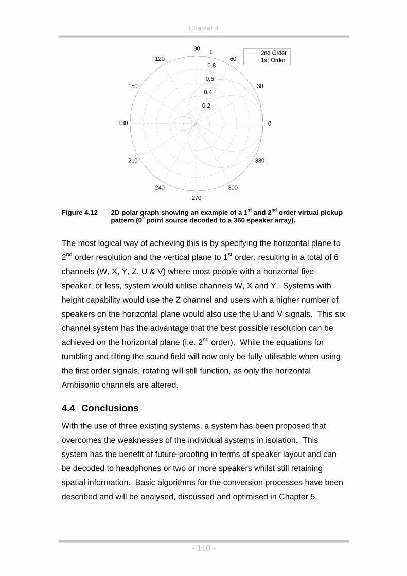
Chapter 4
0.2
0.4
0.6
0.8
1
30
270
60
90
120
210
240 300
330
180 0
2nd Order1st Order
150
Fig
The
2nd d
cha e
peaker, or less, system would utilise channels W, X and Y. Systems with
x
ith the use of three existing systems, a system has been proposed that
n
ure 4.12 2D polar graph showing an example of a 1st and 2nd order virtual pickup pattern (00 point source decoded to a 360 speaker array).
most logical way of achieving this is by specifying the horizontal plane to
or er resolution and the vertical plane to 1st order, resulting in a total of 6
nn ls (W, X, Y, Z, U & V) where most people with a horizontal five
s
height capability would use the Z channel and users with a higher number of
speakers on the horizontal plane would also use the U and V signals. This si
channel system has the advantage that the best possible resolution can be
achieved on the horizontal plane (i.e. 2nd order). While the equations for
tumbling and tilting the sound field will now only be fully utilisable when using
the first order signals, rotating will still function, as only the horizontal
Ambisonic channels are altered.
4.4 Conclusions
W
overcomes the weaknesses of the individual systems in isolation. This
system has the benefit of future-proofing in terms of speaker layout and can
be decoded to headphones or two or more speakers whilst still retaining
spatial information. Basic algorithms for the conversion processes have bee
described and will be analysed, discussed and optimised in Chapter 5.
- 110 -

Chapter 5
Chapter 5 - Surround Sound Optimisation Techniques
5.1 Introduction
In this chapter a number of optimisation methods w
ill be discussed and
emonstrated so as to maximise the performance of the hierarchical system
e use
er
.
h
l performance of the designed filters, this work is not included.
h
h it
nt
consumer and professional audio equipment (i.e. 5, 6 or 7 channel
d
discussed in Chapter 4. A large part of this research was based upon th
of HRTF data collected by Gardner & Martin (1994) which was used in order
to help quantify and optimise the various decoding stages that are present in
the proposed hierarchical system. The research was carried out in a numb
of stages which also corresponds to the layout of this chapter, as detailed
below:
• Investigation into the use of HRTF data in the analysis of multi-channel
sound reproduction algorithms.
• Optimisation of the Ambisonics decoding signal processing techniques.
• Optimisation of the binaural decoding signal processing techniques.
• Optimisation of the Transaural decoding signal processing techniques
To this end, the first part of this investigation, documented in section 5.2, was
to carry out a listening test, using the Multi-Channel Research Lab designed
and installed as part of this research (Schillebeeckx et al., 2001), to try and
measure the potential strengths and weaknesses of the proposed HRTF
analysis technique. As the listening tests were executed before the researc
into the Ambisonic optimisation methods were carried out, sub-optimal
Ambisonic decodes were used in these tests. Also, as work had only just
begun on the Transaural processing techniques, and due to the extremely
sub-optima
Section 5.3 represents the bulk of this chapter, and concentrates on the
optimisation of the Ambisonics system, as this is the base system from whic
the binaural and transaural representations will be derived from. Althoug
would be preferable to always derive the binaural/transaural feeds from the
original B-format (or higher order) carrier, due to the standards used in curre
- 111 -

Chapter 5
presentation for a 5, 6 or 7 speaker, irregular array) it is necessary to realise
optimised Ambisonic decoders for irregular arrays not only to maximise the
performance of the speaker decode, but to also make sure that the correct
irregular decode is
is an
a
e ITU
ay
e,
jekt
on-linear simultaneous equations,
were difficult to solve, and only got more difficult when more speakers were
is reason one of the main aims of this
peaker
. After
on
tly
ork carried out on both Binaural and Transaural
production techniques. The work on binaural reproduction is used as an
e
psychoacoustic cues are presented to a listener after this
converted to a binaural or transaural reproduction.
The original optimisation, as proposed by Gerzon & Barton (1992)
extension of the original Ambisonic energy and velocity vector theory used to
optimise regular decoders (Gerzon, 1977a) but with the added suggestion of
using one decoder for low frequencies and another for high frequencies.
However, although Gerzon and Barton (1992) did solve these equations for
number of irregular speaker arrays, none of the arrays were similar to th
standard array that was finally proposed. No decoders optimised in this w
have ever been produced for the ITU standard speaker array since that tim
as was evident in the recent Project Verdi Listening Tests (Multi Media Pro
Verdi, 2002). The equations, a set of n
added (Gerzon & Barton, 1992). For th
work was to devise a system so that Ambisonic decoders for irregular s
arrays could be easily designed via some form of automated system
this was successfully implemented, the analysis method suggested in earlier
work (see Wiggins et al, 2001) was used as the basis of new optimisation
criterion for irregular Ambisonic decoders. As no method of differentiati
between decoders optimised using the energy/velocity vector model curren
exists (there are multiple solutions), this new method could then be used as a
method to differentiate between already designed velocity/energy vector
decoders.
Section 5.4 documents the w
re
introduction to inverse filtering techniques, which are then applied to the
Transaural reproduction system in order to improve its performance using th
freely available HRTF data from MIT Media Lab (Gardner & Martin, 1994).
- 112 -

Chapter 5
5.2 The Analysis of Multi-channel Sound Reproduction Algorithms Using HRTF Data
5.2.1 The Analysis of Surround Sound Systems
Much research has been carried out into the performance of multi-channel
ound reproduction algorithms, both subjectively and objectively. Much of the
scribed using Head Related Transfer
unctions as a reference for the localisation cues needed to successfully
will then be compared to results
Ch Laboratory.
5.2
sis is that of simple
comparison. If a real source travels through 3600 around the head
d pressure level at both ears is recorded, then the
89;
nt path lengths, the
vel difference between the sounds arriving at each ear due to different path
f complex level
y. The most
the use of Head
or the purpose of this analysis technique, the binaural synthesis of virtual
ed
does not necessarily need to be optimal for all listeners (which can be an
s
quantitative data available on the subject has been calculated by
mathematically simulating acoustical waves emitting from a number of fixed
sources (speakers) (Bamford, 1995) or using mathematical functions that give
an indication of the signals reaching the listener (Gerzon, 1992b). The
resulting sound field can then be observed. In this section of Chapter 5, a
new method of analysis will be de
F
localise a sound in space. This method
obtained from a listening test carried out at the University of Derby’s Multi-
annel Sound Research
.2 Analysis Using HRTF Data
The underlying theory behind this method of analy
(horizontally) and the soun
three widely accepted psychoacoustic localisation cues (Gulick et al., 19
Rossing, 1990) can be observed. These consist of the time difference
between the sounds arriving at each ear due to differe
le
lengths and body shadowing/pinna filtering, a combination o
and time differences due to the listeners own pinna and bod
accurate way to analyse and/or reproduce these cues is with
Related Transfer Functions.
F
sound sources is taken as the reference system, as the impulse responses
used for this system are of real sources in real locations. The HRTF set us
- 113 -

Chapter 5
issue for binaural listening) so long as all of the various localisation cues can
be easily identified. This is the case because this form of analysis compares
the difference between real and virtual sources and as all systems will be
synthesised using the same set of HRTFs, their performance when compared
to another set of HRTFs should not be of great importance.
Once the system has been synthesised using HRTFs, impulse responses can
be calculated for virtual sources from any angle so long as the panning laws
for the system to be tested are known. Once these impulse responses have
been created the three parameters used for localisation can be viewed and
s able to
produce accurate virtual images.
y
can be made between very different multi-channel
systems as long as the HRTFs used to analyse the systems are the same.
rm of
nalysis, a listening test was carried out. The listening test comprised of a set
The tests were carried out in the University of Derby’s Multi Channel Sound
Research Laboratory with the speakers arranged as shown in Figure 5.1.
compared, with estimations made as to how well a particular system i
Advantages of this technique include:
• All forms of multi-channel sound can potentially be analysed meaningfull
using this technique.
• Direct comparisons
• Systems can be auditioned over headphones.
5.2.3 Listening Tests
In order to have a set of results to use as a comparison for this fo
a
of ten tests for five different forms of surround sound:
• 1st Order Ambisonics over 8 speakers (horizontal only)
• 2nd Order Ambisonics over 8 speakers (horizontal only)
• 1st Order Ambisonics over a standard 5 speaker layout.
• Amplitude panned over a standard 5 speaker layout.
• Transaural reproduction using two speakers at +/- 50.
- 114 -
Chapter 5
Figure 5.1 Speaker Arrangement of Multi-channel Sound Research Lab.
The listing room has been acoustically treated and a measurement of the
ambient noise in the room gave around 43 dBA in most 1/3-octave bands,
with a peak at 100 Hz of 52.1 dBA and a small peak at 8 kHz of 44.4 dBA.
The RT60 of the room is 0.42 seconds on average, but is shown in 1/3-octave
bands in Figure 5.17.
Using a PC and a multi-channel soundcard (Soundscape Mixtreme) all of the
speakers could be accessed simultaneously (Schillebeeckx et al., 2001), if
needed, and so tests on all of the systems could be carried out in a single
session without any pauses or equipment changes/repatching.
rks,
.
A flexible framework was devised using Matlab and Simulink (The Mathwo
2003) so that listening test variables could be changed with minimal effort,
with the added bonus that the framework would be reusable for future tests
A Simulink ‘template’ file was created for each of the five systems that could
take variables from the Matlab workspace, such as input signal, overall gain
and panning angle, as shown in Figure 5.2. Then a GUI was created where
all of the variables could be entered and the individual tests run. A screen
shot of the final GUI is shown in Figure 5.3.
- 115 -

Chapter 5
Figure 5.2 Screen shot of two Simulink models used in the listening tests.
Figure 5.3 Screen shot of listening test GUI.
The overall gain parameter was included so each of the different systems
onf
ter
h
could be c igured to have a similar subjective gain, with the angle of the
virtual source specified in degrees. The only exception to this was the 5.0
Amplitude panned system where the speaker feeds were calculated off line
using the Mixtreme soundcards internal mixing feature. The extra parame
(tick box) in the Stereo Dipole (transaural) section was used to indicate whic
side of the listener the virtual source would be placed as the HRTF set used
(Gardner & Martin, 1994) only had impulse responses for the right
hemisphere and must be reversed in order to simulate sounds originating
from the left (indicated by a tick).
- 116 -

Chapter 5
After consulting papers documenting listening tests of various multi-channel
sound systems, it was found that noise (band-limited and wide-band) was
often used as a testing source (see Moller et al., 1999, Kahana et al., 1997
Nielsen, 1991 Orduna et al., 1995 and Zacharov et al, 1999, as typical
examples). The noise signals used in this test were band limited and pulsed,
three pulses per signal, with each pulse lasting two seconds with one sec
of silence between each pulse. The pulsed noise was chosen as it was more
easily localised
,
ond
in the listening room when compared to steady state noise.
Each signal was band limited according to one of the three localisation
frequency ranges taken from two texts (Gulick et al., 1989; Rossing, 1990).
These frequencies are not to be taken as absolutes, just a starting point for
this line of research. A plot of the frequency ranges for each of the three
signals is shown in Figure 5.4.
Figure 5.4 Filters used for listening test signals.
re used, most of whom had never taken part in a
all enrolled on the 3rd year of the
niversity’s Music Technology and Audio System Design course, and so
xperience of the systems at this point. Each listener was asked to
y to move their head as little as possible while listening (i.e. don’t face the
in
listeners were not fixed and so small head movements would have been
Twenty eight test subjects we
listening test before. The test subjects were
U
knew the theory behind some surround sound systems, but had little or no
listening e
tr
source), and to indicate the direction of the source by writing the angle,
degrees, on an answer paper provided. It must be noted that the head of the
- 117 -

Chapter 5
available to the listeners as a potential localisation cue (as it would be when
listening anyway). Listeners could ask to hear a signal again if they
needed
, and the operator only started the next signal after an answer had been
re
.5 (although the sheet presented to the test subjects was labelled in 50
intervals with a tick size of 10, not 150 intervals with a tick size of 30 as shown
in Figure 5.5).
to
recorded. The listeners were given a sheet of paper to help them with angle
locations with all of the speaker positions marked in a similar fashion to Figu
5
0
180
270 90
300
330
60
30
120
150210
240
15
45
285
225
255
135
105
195 165
75
315
345 0
180
270 90
300
330
60
30
120
150210
240
15
45
285
225
255
135
105
195 165
75
315
345
as
Order Ambisonics
• 2nd Order Ambisonics
• 1st Order Ambisonics over 5 speakers.
The listening test results for the amplitude panned 5 speaker system are also
included.
The set of HRTFs used for this anal
HRTFs, specifically the compact set (Gardner & Martin, 1994). As m
Figure 5.5 Figure indicating the layout of the listening room given to the testees
a guide to estimating source position.
5.2.4 HRTF Simulation
As described in section 5.1 three of the five systems will be analysed using
the HRTF method described above:
• 1st
ysis were the MIT media lab set of
entioned
- 118 -

Chapter 5
earlier, it is not necessarily important that these are not the best HRTF set
available, just that all of the localisation cues are easily identifiable.
All systems can be simulated binaurally but Ambisonics is a slightly special
case as it is a matrixed system comprising the steps shown in Figure 5.6.
W X Y
Ambisonic
HRTF Decoder
Left Ear
Simulation Right Ear
ividual HRTFs are needed
for any speaker arrangement, Equation (5.1). If the head is assumed to be
symmetrical (which it is in the MIT set of compact HRTFs) then even fewer
HRTFs are needed as Wleft and Wright will be the same (Ambisonics omni-
directional component), Xleft and Xright will be the same (Ambisonics
front/back component) and Yleft will be phase inverted with respect to Yright.
This means a complete 1st order Ambisonic system comprising any number of
speakers can be simulated using just three HRTF filters, as shown in equation
(5.1).
Figure 5.6 The Ambisonic to binaural conversion process.
Because the system takes in three channels which are decoded to eight
speaker feeds, which are then decoded again to two channels, the
intermediate decoding to eight speakers can be incorporated into the HRTFs
calculated for W, X and Y meaning that only six ind
( ) ( )( ) ( )( )
∑ ==
8
1
hrtf
khrtfk
hrtf SW
( ) ( )( )∑=
×=8
1
sinsin hrtfhrtf
k kkk
SY φθ
Where θ = source azimuth φ = source elevation (0 for horizontal only)Sk
hrtf = Pair of Speakers positional HRTFs.
∑ ×=
×8 sincos
2
kkk
hrtf SX φθ
5.1)
=1k
(
- 119 -
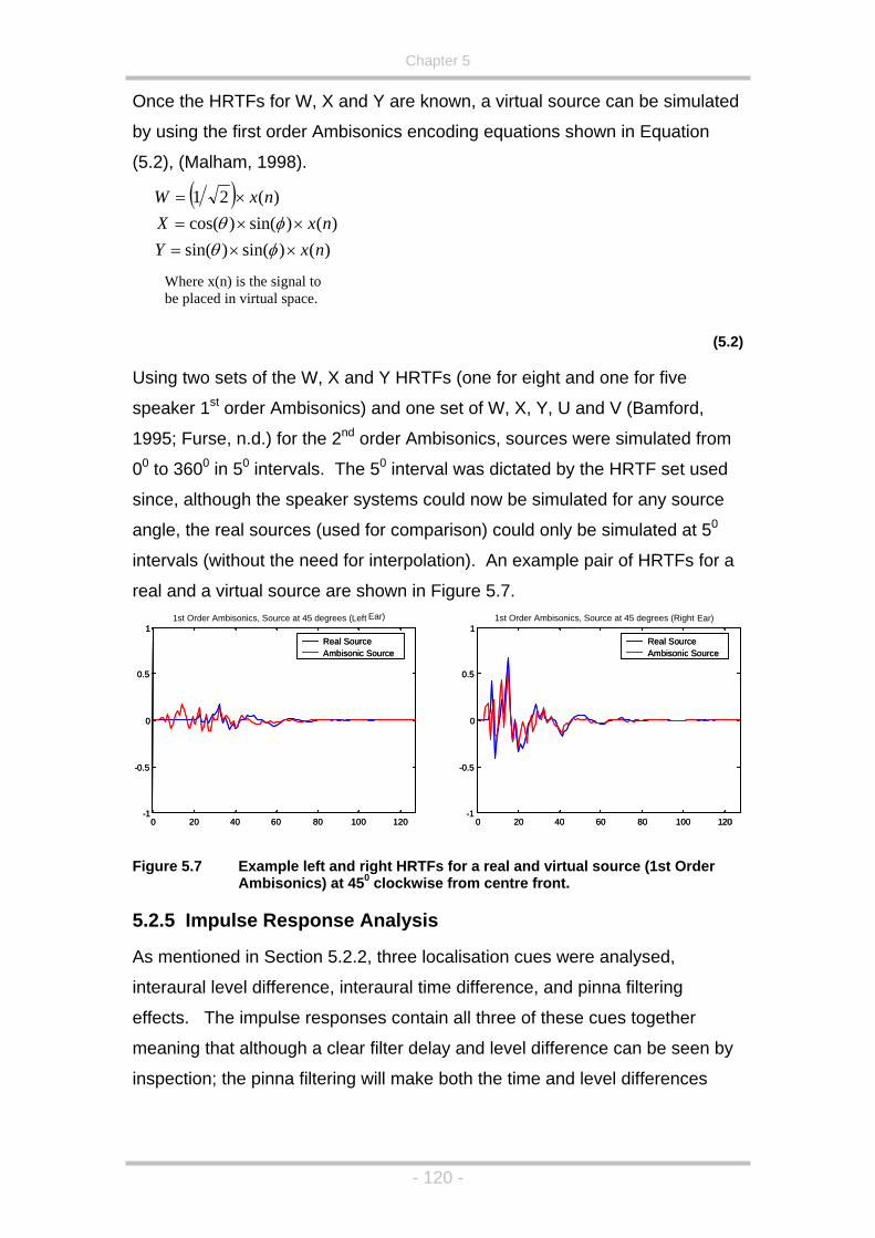
Chapter 5
Once the HRTFs for W, X and Y are known, a virtual source can be simulated
by using the first order Ambisonics encoding equations shown in Equation
(5.2), (Malham, 1998).
( ) )(21 nxW ×=
)()sin()sin()()sin()cos(
nxYnxX
××=××=
φθφθ
Where x(n) is the signal to be placed in virtual space.
(5.2)
rce
50
n in Figure 5.7.
Using two sets of the W, X and Y HRTFs (one for eight and one for five
speaker 1st order Ambisonics) and one set of W, X, Y, U and V (Bamford,
1995; Furse, n.d.) for the 2nd order Ambisonics, sources were simulated from
00 to 3600 in 50 intervals. The 50 interval was dictated by the HRTF set used
since, although the speaker systems could now be simulated for any sou
angle, the real sources (used for comparison) could only be simulated at
intervals (without the need for interpolation). An example pair of HRTFs for a
real and a virtual source are show
Figure 5.7 Example left and right HRTFs for a real and virtual source (1st Order Ambisonics) at 450 clockwise from centre front.
5.2.5 Impulse Response Analysis
As mentioned in Section 5.2.2, three localisation cues were analysed,
interaural level difference, interaural time difference, and pinna filtering
effects. The impulse responses contain all three of these cues together
meaning that although a clear filter delay and level difference can be seen by
inspection; the pinna filtering will make both the time and level differences
20 40 60 80 100 12020 40 60 80 100 120 20 40 60 80 100 2020 40 60 80 100 1200 - 1
- 0.5
0
0.5
1 1st Order Ambisonics, Source at 45 degrees (Left Real SourceAmbisonic Source
0 - 1
- 0.5
0
0.5
1 Ear) Real SourceAmbisonic Source
0 1-1
-0.5
0
0.5
11st Order Ambisonics, Source at 45 degrees (Right
Real Source Ambisonic Source
0 -1
-0.5
0
0.5
1Ear)
Real Source Ambisonic Source
- 120 -
Chapter 5
frequency dependant. These three cues were extracted from the HRTF data
using the following methods:
• Interaural Amplitude Difference – Mean amplitude difference between th
two ears, taken from an FFT of the impulse responses.
• Interaural Time Difference – Mean time difference between the two e
taken from the group delay of the impulse responses.
• Pinna filtering – Actual time and amplitude values, taken from the
delay and an FFT of the impulse responses.
Once the various psychoacoustic cues had been separated, compariso
were made between the cues present in a multi-speaker decode com
with the cues of an actual source (i.e. the individual HRTFs) and estimations
of where the sounds may appear to come from can be made using each of
the localisation parameters in turn. As the
e
ars,
group
ns
pared
analysis is carried out in the
frequency domain, band limiting the results (to coincide with the source
material used in the listening tests) is simply the case of ignoring any data that
is outside the range to be tested.
As an example, Figure 5.8 shows the low, mid and high frequency results for
real sources and the three Ambisonic systems for averaged time and
amplitude differences between the ears.
These graphs show a number of interesting points about the various
Ambisonic systems. Firstly, the 2nd order system actually has a greater
amplitude difference between the ears at low frequencies when compared to
a real source, and this is also the frequency range where all of the systems
seem to correlate best with real sources. However, the ear tends to use
amplitude cues more in the mid frequency range, and another unexpected
result was also discovered here. It seems that the 1st order, five speaker
system actually outperforms the 1st order, eight speaker system at mid
frequencies, and seems to be equally as good as the eight speaker, second
order system. This is not evident in the listening tests, but if the average time
difference graphs are observed it can be seen that the five speaker system
has a number of major errors around the 900 and 2700 source positions and
- 121 -

Chapter 5 Chapter 5
- 122 -
shows the 2nd order system to hold the best correlation. The time difference
plots all show that the five speaker system still outperforms the 1st order, eight
speaker system, apart from the major disparities, mentioned above, at low
frequencies. It can be seen from the listening test results (Figure 5.12) that
the five speaker system does seem to be at least as good as the eight
speaker system over all three of the frequency ranges, which was not
expected. The mid and high frequency range graphs are a little too
complicated to analyse by inspection and so will be considered later in this
chapter using a different technique. It must also be noted that, due to the
equency ranges originally chosen, interaural level differences at low
frequencies are comparable to the interaural level differences at mid
frequencies. Had a lower cut off frequency been chosen (as shown later in
this Chapter) this would not have been the case and this suggests that the
original frequency ranges were not ideal.
fr
- 122 -

Chapter 5
0 50 100 150 200 250 300 350 400-1.5
-1
-0.5
0
0.5
1
1.5Low Frequency Amplitude Difference (Average)
Actual5.0 Ambi8 Speak Ambi2nd Order
0 50 100 150 200 250 300 350 400-1.5
-1
-0.5
0
0.5
1
1.5Mid Frequency Amplitude Difference (Average)
Actual5.0 Ambi8 Speak Ambi2nd Order
0 50 10-1.5
-1
-0.5
0
0.5
1
1.5High
0 50 10-80
-60
-40
-20
0
20
40
60
80M
Figure 5.8
Am
plitu
de D
iffer
ence
Am
plitu
de D
iffer
ence
Am
plitu
de D
iffer
ence
Ti
me
Diff
eren
ce
Source Angle (degrees)
0 150 200 250 300 350 400
Frequency Amplitude Difference (Average)
Actual
0 50 100 150 200 250 300 350 400-80
-60
-40
-20
0
20
40
60
80Low Frequency Time Difference (Average)
Actual5.0 Ambi8 Speak Ambi2nd Order
5.0 Ambi8 Speak Ambi2nd Order
0 150 200 250 300 350 400
id Frequency Time Difference (Average)
Actual5.0 Ambi8 Speak Ambi2nd Order
0 50-40
-30
-20
-10
0
10
20
30
40
The average amplitude and time differencmid and high frequency ranges.
Tim
e D
iffer
ence
Ti
me
Diff
eren
ce
- 123 -
Source Angle (degrees)
Source Angle (degrees)
Source Angle (degrees)
100 150 200 250 300 350 400
High Frequency Time Difference (Average)
Actual5.0 Ambi8 Sp2nd O
eak Ambirder
Source Angle (degrees) Source Angle (degrees)es between the ears for low,

Chapter 5
Figure 5.9 The difference in pinna amplitude filtering of a real source and 1 and
2st
e
ent,
an
ple,
the non-averaged amplitude or group delay parameters are looked at over
the full 3600 (the non-averaged amplitude responses are shown in Figure 5.9)
nd order Ambisonics (eight speaker) when compared to a real source.
One attribute that has not really been touched on yet, when discussing multi-
speaker systems, which is one of the major consequences of the phantom
imaging scenario, is pinna cue errors. When an image is created with mor
than one speaker, although it is possible to create a correct level and phase
difference at the ears of a listener, for a panned source, it will be far more
difficult to create correct pinna cues due to the direction dependant filtering
that the pinnae apply to real sound sources. Instead, the pinna cues from the
speakers creating the phantom image will be summed and weighted
dependant on the speakers’ contributions. As everyone’s pinnae are differ
it is impossible to correct for this in a generic way (and even from
individual’s response point of view, only one listener orientation could be
corrected for, i.e., facing straight ahead). The pinna filtering can be clearly
seen in the simulation, but is a more complex attribute to analyse directly,
although it has been useful to look at for a number of reasons. For exam
if
- 124 -
Chapter 5
it can be seen that they both change radically due to virtual source position
(as does a source in reality). However, the virtual sources change differently
when compared to real sources. This change will also occur if the head i
rotated (in the same way as a source moving for a regular rig, or a slightly
more complex way for an irregular five speaker set-up) and this could be p
of the ‘phasiness’ parameter that Gerzon often mentioned in his papers
regarding the problems of Ambisonics (Gerzon, 1992b). This problem,
however, is not strictly apparent as a timbral change (at least, not straight
away) when a source or the listener’s head moves, but instead probably just
aids in confusing the brain as to the sound source’s real location, increasing
source location ambiguity and source mo
s
art
vement when the listener’s head is
rned. This parameter is more easily observed using an animated graph, but
t a
r
further work will be carried out to make use of this
formation. However, using the average time and amplitude differences to
ders
as
t,
shown, using the average
mplitude and the average time differences at low and mid frequencies.
tu
it is shown as a number of stills in Figure 5.9. These graphs show the
differences between the three systems, which is why the ‘real source’ is jus
0dB line, as it has no amplitude difference with itself.
Due to the complexity of the results obtained using the HRTF simulation fo
the pinna filtering, it is difficult to utilise these results in any estimation of
localisation error, although
in
estimate the perceived direction of the virtual sound source is a relatively
trivial task using simple correlation between the actual and virtual sources. In
order to plot these results, a Matlab routine was constructed that gave a
localisation estimation using the HRTFs derived from the various deco
and compared these to the figures obtained from the real HRTFs. This w
carried out for both amplitude and time differences in the various frequency
bands tested. Because no pinna filtering effects were taken into accoun
each value of amplitude and time/phase difference will have two
corresponding possible localisation angles (see the cone of confusion in
chapter 2.2.1). Figure 5.10, Figure 5.11 and Figure 5.12 show the listening
test results with the estimated localisations also
a
- 125 -

Chapter 5
The listening tests themselves gave reasonably expected results as far as to
the system that performed best (the 2
ver
d.
r
y
t
d
of
s long as the speakers
used in each system are matched (as opposed to the speakers across all
ame).
more
of
is a
rce at 00 just radiates from the centre
peaker, i.e. it is a real source at 00. However, around 30% of the subjects
recorded that the source came from behind them. Front/back reversals were
actually less common in all of the other systems (at 00), apart from 2nd order
Ambisonics (the system that performed best).
The source position estimation gave reasonably good results when compared
with the results taken from the listening tests, with any trends above or below
nd Order Ambisonics system). Howe
the other three systems (1st order eight and five speaker, and amplitude
panned 5.0) all seemed to perform equally as well, which was not expecte
Although it must be noted, that all of these listening tests were carried out
using ‘unoptimised’ decoders, with only the five speaker irregular decode
having been empirically adjusted regarding the amplitude levels of the three
speaker sets (centre, front pair and rear pair). Nevertheless, the empiricall
derived gain settings reasonably matched the optimised sets described later
(quiet centre speaker with additional gain applied to the rear pair) but with all
speakers using a cardioid pattern feed.
The speakers used for the eight and five speaker systems were different, bu
as all listeners had the speakers pointed directly at them, and were teste
using band-limited noise, the frequency response and dispersion patterns
the speakers should not have been critical in this experiment. Also, the HRTF
simulation and comparison should be a valid one a
systems being the s
The frequency content of the sounds did not seem to make any significant
difference to the perceived localisation of the sound sources, although a
extensive test would have to be undertaken to confirm this, as the purpose
this test was to test between any large differences between the three
localisation frequency ranges. Another interesting result was the virtual
source at 00 on the amplitude panned system (see Figure 5.13). As there
centre front speaker, a virtual sou
s
- 126 -

Chapter 5
- 127 -
the diagonal, representing a perfect score, being estimated successfully. If
the graphs represented truly what is expected from the different types of
psychoacoustic sound localisation, then the low frequency time graph and the
mid frequency amplitude graph should be the best indicator of where the
source is coming from. However it is well known (Gulick et al., 1989) that if
one localisation cue points to one direction, and the other cue points to
another, then it may be some direction between these two localisation angles
that the sound is actually perceived to originate from. The HRTF analysis
does not take this into account at the moment and so some error is expected.
Also, the compact set of HRTFs used is the minimum phase versions of the
actual HRTFs recorded which may contribute to the time difference estimation
results (although the cues seem reasonable when looked at for the actual
sources). As mentioned, there was no major difference between the three
different signals in terms of localisation error. Because of this the plots
showing the estimated localisation using the whole frequency range are
shown in Figure 5.14 - Figure 5.16 which also show the interaural amplitude
difference as a better localisation approximation.
5.2.6 Summary
The HRTF analysis of the three surround systems described in this section
seems to work well giving a reasonably good indication as to the possible
localisation that a listener will attach to a sound object. This method is
definitely worth pursuing as a technique that can be used to evaluate and
compare all forms of surround sound systems equally. Although the errors
seen in the estimation when compared to the listening test results can be
quite large, the general trends were shown accurately, even with such a
simple correlation model used.

Chapter 5
1st Order Ambisonics
-50
0
50
100
150
200
250
300
350
400
-50 0 50 100 150 200 250 300 350
Low Pass Filtered Signal
Band Pass Filtered Signal
High Pass Filtered Signal
Perc
eive
d An
gle
Actual Source Angle
0
50
100
150
200
250
300
350
400
0 50 100 150 200 250 300 350
-50
0
50
100
150
200
250
300
350
400
-50 0 50 100 150 200 250 300 3500
50
100
150
200
250
300
350
400
0 50 100 150 200 250 300 350
-50
0
50
100
150
200
250
300
350
400
-50 0 50 100 150 200 250 300 350
Source Localisation Estimates using Interaural Amplitude
differences Low Frequency Mid Frequency
Source Localisation Estimates using Interaural Time differences
Low Frequency Mid Frequency
0
50
100
150
200
250
300
350
400
0 50 100 150 200 250 300 350
-50
0
50
100
150
200
250
300
350
400
-50 0 50 100 150 200 250 300 3500
50
100
150
200
250
300
350
400
0 50 100 150 200 250 300 350
-50
0
50
100
150
200
250
300
350
400
-50 0 50 100 150 200 250 300 350
Figure 5.10 Listening Test results and estimated source localisation for 1st Order Ambisonics
- 128 -
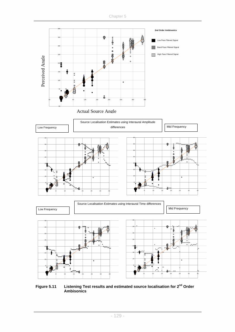
Chapter 5
Source Localisation Estimates using Interaural Amplitude
differences Low Frequency Mid Frequency
0
50
100
150
200
250
300
350
400
0 50 100 150 200 250 300 350 0
50
100
150
200
250
300
350
400
0 50 100 150 200 250 300 350
Figure 5.11 ated source localisation for 2 Order
Ambisonics
Source Localisation Estimates using Interaural Time differences
Low Frequency Mid Frequency
0
50
100
150
200
250
300
350
400
0 50 100 150 200 250 300 350 0
50
100
150
200
250
300
350
400
0 50 100 150 200 250 300 350
Low Pass Filtered Signal
Band Pass Filtered Signal
High Pass Filtered Signal
2nd Order Ambisonics
-50
0
50
100
150
200
250
300
350
400
-50 0 50 100 150 200 250 300 350
Low Pass Filtered Signal
Band Pass Filtered Signal
High Pass Filtered Signal
Perc
eive
d A
ngle
Actual Source Angle
Listening Test results and estim nd
- 129 -
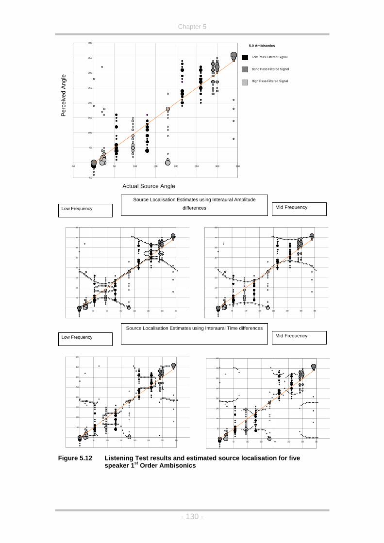
Chapter 5
Figure 5.12 Listening Test results and estimated source localisation for five
speaker 1st Order Ambisonics
5.0 Ambisonics
-50
0
50
100
150
200
250
300
350
400
-50 0 50 100 150 200 250 300 350
Low Pass Filtered Signal
Band Pass Filtered Signal
High Pass Filtered Signal
Perc
eive
d An
gle
Actual Source Angle
Source Localisation Estimates using Interaural Amplitude
differences Low Frequency Mid Frequency
0
50
100
150
200
250
300
350
400
0 50 100 150 200 250 300 3500
50
100
150
200
250
300
350
0 50 100 150 200 250 300 350
400
Source Localisation Estimates using Interaural Time differences
Low Frequency Mid Frequency
0
50
100
150
200
250
300
350
400
0 50 100 150 200 250 300 3500
50
100
150
200
250
300
350
400
0 50 100 150 200 250 300 350
- 130 -

Chapter 5
Figure 5.14 Average Time and Frequency Localisation Estimate for 1st Order
Figure 5.13 Listening test results for Amplitude Panned five speaker system.
Amplitude Panned 5.0
-50
0
50
100
150
200
250
300
350
400
-50 0 50 100 150 200 250 300 350
Low Pass Filtered Signal
Band Pass Filtered Signal
High Pass Filtered Signal
Perc
eive
d So
urce
Actual Source Angle
0
50
100
150
200
250
300
350
400
0 50 100 150 200 250 300 3500
50
100
150
200
250
300
350
400
0 50 100 150 200 250 300 350
Average Time difference
Average Amplitude difference
Ambisonics.
- 131 -

Chapter 5
- 132 -
Figure 5.15 Average Time and Frequency Localisation Estimate for 2nd Order
Ambisonics.
Average Time and Frequency Localisation Estimate for five speaker 1st
Order Ambisonics.
Low Pass Fi ltered Signal
Band Pass Filtered Signal
High Pass Filtered Signal
2nd Order Ambisonics
Low Pass Filtered Signal
Band Pass Filtered Signal
High Pass Filtered Signal
0
50
100
150
200
250
300
350
400
0 50 100 150 200 250 300 3500
50
100
150
200
250
300
350
400
0 50 100 150 200 250 300 350
Average Time difference
Average Amplitude difference
5.0 Ambisonics
ass Filtered Signal
ass Filtered Signal
High Pass Filtered Signal
300
400
Figure 5.16
Low P
Band P
0
50
100
150
200
0 50 100 150 200 250 300 350
250
350
300
400
350
250
Average Time difference
0
50
100
150
200
0 50 100 150 200 250 300 350
Average Amplitude difference

Chapter 5
RT60 For Multi-channel SoundResearch Laboratory.
0.40
0.50
0.60
0.70
0.80
0.90
1.00R
T60
(sec
onds
)
0.00
0.10
0.20
0.30
Frequency (kHz)RT60 Time (s) 0.65 0.65 0.65 0.50 0.45 0.30 0.30 0.30 0.35 0.35 0.35 0.35 0.40 0.55 0.45 0.40 0.35 0.30 0.35 0.30
0.125 0.160 0.200 0.250 0.315 0.400 0.500 0.630 0.800 1.000 1.250 1.600 2.000 2.500 3.150 4.000 5.000 6.300 8.000 10.000
Figure 5.17 RT60 Measurement of the University of Derby’s multi-channel sound
research laboratory, shown in 1/3 octave bands.
5.3 Optimisation of the Ambisonics system
.3.1 Introduction
that the virtual microphone response for the decoder (he concentrated on
regular setups initially) should be chosen according to a number of
5
In this part of the chapter the decoding techniques that have been utilised in
the system described in Chapter 4 (Ambisonics, binaural and transaural) will
be discussed and optimised so as to both maximise their spatial performance
and sound quality. Some of these optimisations are more logically formulated
than others, with the optimisation of the Ambisonics system being the most
involved, both mathematically and perceptually, so this system will be
considered first.
As discussed in Chapter 4, the Ambisonics system will be the basis for the
proposed hierarchical multi-channel system, but while the encoding process is
a fixed standard (using the spherical harmonics described in Chapter 3) the
decoding process is not necessarily as straightforward. As the Ambisonics
system is very flexible, any 1st order microphone response can be chosen,
along with the virtual microphone’s direction. Gerzon’s original theory stated
- 133 -
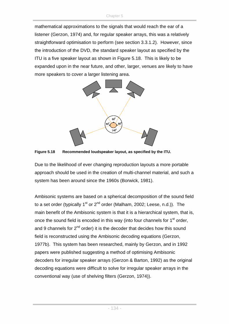
Chapter 5
mathematical approximations to the signals that would reach the ear of a
he
ave
listener (Gerzon, 1974) and, for regular speaker arrays, this was a relatively
straightforward optimisation to perform (see section 3.3.1.2). However, since
the introduction of the DVD, the standard speaker layout as specified by t
ITU is a five speaker layout as shown in Figure 5.18. This is likely to be
expanded upon in the near future, and other, larger, venues are likely to h
more speakers to cover a larger listening area.
600
1400
800 800
600
1400
800 800
Figure 5.18 Recommended loudspeaker layout, as specified by the ITU.
e likelihood of ever changing reproduction layouts a more portable
, and such a
e the 1960s (Borwick, 1981).
mbisonic systems are based on a spherical decomposition of the sound field
he
hat is,
rched, mainly by Gerzon, and in 1992
apers were published suggesting a method of optimising Ambisonic
decoders for irregular speaker arrays (Gerzon & Barton, 1992) as the original
decoding equations were difficult to solve for irregular speaker arrays in the
conventional way (use of shelving filters (Gerzon, 1974)).
Due to th
approach should be used in the creation of multi-channel material
system has been around sinc
A
to a set order (typically 1st or 2nd order (Malham, 2002; Leese, n.d.)). T
main benefit of the Ambisonic system is that it is a hierarchical system, t
once the sound field is encoded in this way (into four channels for 1st order,
and 9 channels for 2nd order) it is the decoder that decides how this sound
field is reconstructed using the Ambisonic decoding equations (Gerzon,
1977b). This system has been resea
p
- 134 -

Chapter 5
5.3.2 Irregular Ambisonic Decoding
In order to quantify decoder designs Gerzon decided on two main criteria for
designing and evaluating multi-speaker surround sound systems in terms of
their localisation performance. These represent the energy and velocity
vector components of the sound field (Gerzon, 1992c). The vector lengths
represent a measure of the ‘quality’ of localisation, with the vector angle
representing the direction that the sound is perceived to originate from, with a
vector length of one indicating a good localisation effect. These are evaluated
as shown in Equation (5.3)
( )
( )∑
∑
=
=
=
=
=
n
iii
i
n
ii
PgVy
gP
0
0
1
sin
os
θ
∑=n
ii PgVx c θ ( )
( )∑
∑
=
=
=
=
iii
n
ii
EgEy
gE
0
2
1
2
sin θ
(5.3)
Where:
gi represents the gain of a speaker (assumed real for simplicity).
n is the number of speakers.
θi is the angular position of the ith speaker.
For regular speaker arrays, this was simply a case of using one virtual
microphone response for low frequencies and a slightly different virtual
microphone response for the mid and high frequencies by the use of shelving
filters (Farino & Uglotti, 1998) as shown in Figure 5.19 and Figure 5.20. This
equalisation d
∑=
=
n
n
iii EgEx
0
2 cos θ
is extremely similar to the theory and techniques used by Blumlein’s spatial
escribed in Chapter 2.
- 135 -
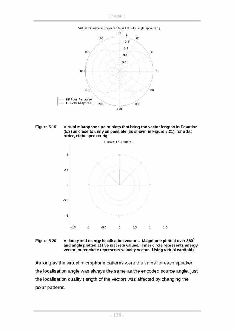
Chapter 5
0.2
0.4
0.6
0.8
1
30
210
60
240
90
270
120
300
150
330
180 0
Virtual microphone responses for a 1st order, eight speaker rig
HF Polar ResponseLF Polar Response
Figure 5.19 Virtual microphone polar plots that bring the vector lengths in Equation
(5.3) as close to unity as possible (as shown in Figure 5.21), for a 1st order, eight speaker rig.
-1.5 -1 -0.5 0 0.5 1 1.5
-1
-0.5
0
0.5
1
D low = 1 D high = 1
Figure 5.20 Velocity and energy localisation vectors. Magnitude plotted over 3600
and angle plotted at five discrete values. Inner circle represents energy vector, outer circle represents velocity vector. Using virtual cardioids.
As long as the virtual microphone patterns were the same for each speaker,
the localisation angle was always the same as the encoded source angle, just
the localisation quality (length of the vector) was affected by changing the
polar patterns.
:
- 136 -
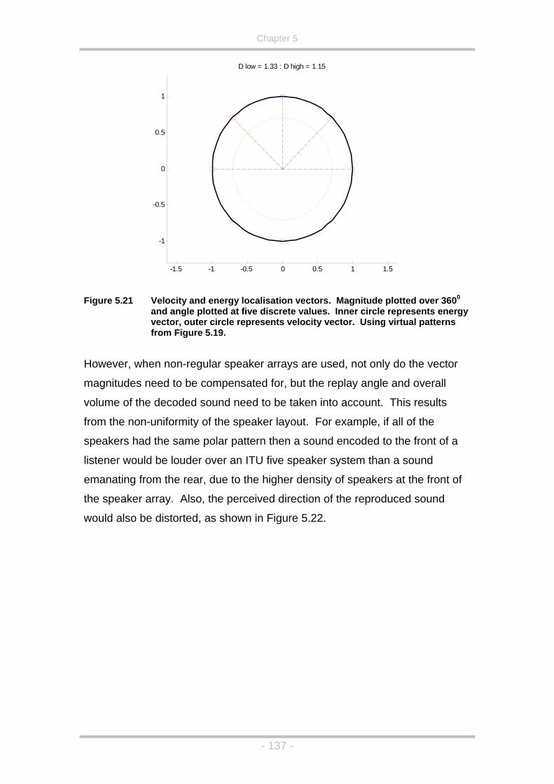
Chapter 5
-1.5 -1 -0.5 0 0.5 1 1.5
-1
-0.5
0
0.5
1
D low = 1.33 : D high = 1.15
Figure 5.21 Velocity and energy localisation vectors. Magnitude plotted over 3600
and angle plotted at five discrete values. Inner circle represents energy vector, outer circle represents velocity vector. Using virtual patterns
stener would be louder over an ITU five speaker system than a sound
from Figure 5.19.
However, when non-regular speaker arrays are used, not only do the vector
magnitudes need to be compensated for, but the replay angle and overall
volume of the decoded sound need to be taken into account. This results
from the non-uniformity of the speaker layout. For example, if all of the
speakers had the same polar pattern then a sound encoded to the front of a
li
emanating from the rear, due to the higher density of speakers at the front of
the speaker array. Also, the perceived direction of the reproduced sound
would also be distorted, as shown in Figure 5.22.
- 137 -

Chapter 5
SpeakersVelocity Vector
Energy Vector
0,12.25,22.5, 45,90 & 135 degrees reproduced angles
Energy and veFigure 5.22 locity vector response of an ITU 5-speaker system, using virtual cardioids.
xed
any speaker layouts as possible, these artefacts must be
orrected after the encoding has occured, that is, during the decoding stage.
Due to the added complexity of the speaker array’s response to an Ambisonic
system, G on and Barton (1992) proposed that two separate decoders be
used, one for low frequency (<~700Hz) and another for high frequencies
(>~700 Hz). This can be achieved using a simple cross-over network feed
ecoders. It is also important that the cross-over filters are perfectly phase
igure
.23, and comprises of an omni-directional pressure signal (W), a front-back
These artefacts are not a problem when you are producing audio for a fi
setup (i.e. amplitude panned 5.1) as material is mixed so it sounds correct on
the chosen speaker layout. However, as the point of using a hierarchical
surround sound format is that an audio piece should sound as similar as
possible on as m
c
erz
ing
low and high passed versions of the Ambisonic B-format signals to the two
d
matched so that the reinforcement and cancellation principles used by
Ambisonics still function correctly.
5.3.3 Decoder system
1st order Ambisonics is comprised of four different signals, as shown in F
5
- 138 -
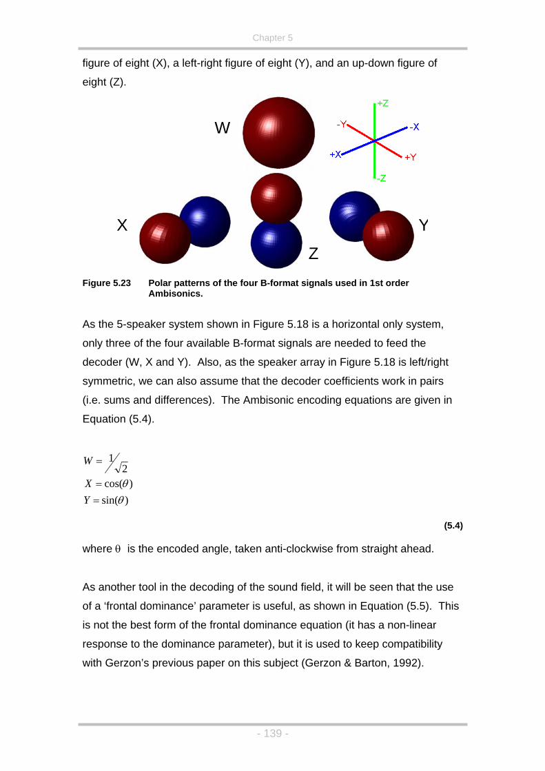
Chapter 5
figure of eight (X), a left-right figure of eight (Y), and an up-down figure of
eight (Z).
W
X Y Z
Figure 5.23 Polar patterns of the four B-format signals used in 1st order
Ambisonics.
As the 5-speaker system shown in Figure 5.18 is a horizontal only system,
only three of the four available B-format signals are needed to feed the
decoder (W, X and Y). Also, as the speaker array in Figure 5.18 is left/right
symmetric, we can also assume that the decoder coefficients work in pairs
(i.e. sums and differences). The Ambisonic encoding equations are given in
Equation (5.4).
)cos(2
1
θ=
=
X
W
)θY sin(=
5.4)
where θ is ht ahead.
s another tool in the decoding of the sound field, it will be seen that the use
ter), but it is used to keep compatibility
ith Gerzon’s previous paper on this subject (Gerzon & Barton, 1992).
(
the encoded angle, taken anti-clockwise from straig
A
of a ‘frontal dominance’ parameter is useful, as shown in Equation (5.5). This
is not the best form of the frontal dominance equation (it has a non-linear
response to the dominance parame
w
- 139 -

Chapter 5
( ) ( )( ) ( )
YYW
′
(5.5)
where λ is the forward dominance parameter (>1 for front, and <1 for rear
dominance).
These encoding equations are then substituted into the decoding equations to
give a numerical value for each speaker’s output to a particular signal as
given in Equation (5.6). In this equation it can be seen that what were
previously sine and cosine (i.e. directionally dependant) weightings are now
arbitrary values (nominally to be chosen between 0 and 1), denoted by kW,
kX and kY.
)YYYkYXkXWYkYXkXWkWL
XkXWkWC
FFF
FFFF
CCF
′′′′′×−′×+′×
′×+′×+′×=
′×+′×=
)())()()()(
(5.6)
here fficient (e.g. kWc represents the weighting
iven to the W channel for centre front speaker).
er’s
ing
XX −++=′ −− 121 25.0 λλλλ
XWW −++=′
−
−−−
1
121
1 85.0 λλλλ
=
( )( )( )
kWRF = (
(kYXkXWkWRkYXkXWkWL BBBB
×−′×+′×=×+×+×=
)()()()(
BBBB
w k denotes a decoding coe
g
F, B and C denote front, back and centre speakers respectively.
W’,X’ and Y’ represent the incoming B-format signals after potential
transformation by the forward dominance equation.
C, L and R denote centre, left and right speakers
The values for λ and the ‘k’ values are to be chosen to optimise the decod
output, with λ having possible values between 0 and 2, and ‘k’ values hav
a nominal range between 0 and 1.
Equation (5.7) shows the conditions which are used to assess the
performance of a given solution. The conditions that must be met are:
- 140 -

Chapter 5
Radius of the localisation vector lengths (RV and RE) should be as close to 1
as possible for all values of θ.
θ = θV=θE for all values of θ.
PV=PE and must be constant for all values of θ.
∑ ×=N
Vii PSPosgVx )cos(=i 1
∑
∑
∑
=
=
=
×=
×=
×=
N
iEii
N
iEii
N
iVii
PSPosgEy
PSPosgEx
PSPosgVy
1
2
1
2
1
)sin(
)cos(
)sin(
( )22
22
yxV
yxE
VVR
EER
+=
+= ( )xyV
xyE
VV
EE1
1
tan
tan−
−
=
=
θ
θ
∑=
=n
iiV gP
1
∑=
A system that can automatically calculate decoder coefficients is needed, and
possibly one that can distinguish between sets of coefficients that meet the
=n
iiE gP
1
2
(5.7)
where:
gi = Gain of the ith speaker
SPosi = Angular position of the ith speaker.
V denotes velocity vector
E denotes energy vector
The reason that these equations are difficult to solve is that the best result
must be found over the whole listening area, spanning 3600. Even Gerzon
admitted that these equations were laborious to solve for five speakers, and
the more speakers present, i.e. the more values that must be optimised, the
more laborious and time consuming finding the solution becomes. Also, there
is more than one valid solution for each decoder (low frequency and high
frequency) meaning that a group of solutions need to be found, and then
auditioned, to determine the best set of coefficients.
- 141 -

Chapter 5
criteria set out by the energy and velocity vector theories. This system does
not need to be particularly fast, as once a group of solutions are found the
program should not need to be used again, unless the speaker layout
changes.
5.3.4 The Heuristic Search Methods
As a result of the fact that each parameter in the Ambisonic decoding
equations will have a value within a well defined range, 0 to 1 or 0 to 2, a
search method offers an effective solution to the array optimisation problem.
owever, if we wish to determine the settings to two decimal places there are
ost
od the measure of the success of its choice. Care must be taken when
cho i ible for different error
con ti gical solution to this
pro t
number. The fitness equations developed for this project are described later
ed on
hen
rmed
H
2 x 10¹⁸ possible solutions (given that there are 9 search parameters) and an
exhaustive search is not feasible (Wiggins et al, 2003). When deciding on
the type of heuristic method, an empirical approach was used. The m
important part of any heuristic search method is the development of the
fitness equations. These are the functions that give the heuristic search
meth
os ng these functions to make sure that it is not poss
di ons to cancel each other out with the most lo
blem being to ensure that any error in the decode resul s in a positive
in this chapter. The first avenue of research taken was that of a Genetic
Algorithm approach, as this is one of the better known heuristic methods.
This was first implemented as a Matlab script and did not seem to converge to
a good result, so the next system to try was one using an algorithm bas
the Tabu search as this has been shown to converge more accurately w
used in a small search space (Berry, S. & Lowndes V., 2001). It was while
developing this algorithm that it was discovered that the initial velocity and
energy vector calculations contained errors, and once corrected, the Tabu
search algorithm performed as expected. As this tabu algorithm perfo
well, the genetic algorithm was not tried again at this point due to its known
convergence problems as described above (Genetic Algorithms are better
suited to a very large search space, which this problem did not have).
- 142 -
Chapter 5
This adapted form of Tabu search works by having the decoder coef
initialised at random values (or values of a
ficients
previous decoder, if these values
re to be optimised further). Then the Tabu search program tries changing
each of the ‘tweakable’ values, plus or minus the step size. The best result is
then kept and the parameter changed is then restricted to only move in the
successful direction for a set number of iterations (which, of course, will only
happen if this parameter, again, is the best one to move). It must be noted
that the random start position is of great importance, as it is this that helps in
the search for a wide range of solutions.
The most important part of the Tabu search algorithm is the equations used to
measure the fitness of the decoder coefficients, as it is this one numerical
at will determine the course that the Tabu search takes. As
mentio equation that
repres ented. These
are:
• Localisation measure (vector lengths, R
•
• ded
.
As each of the parameters must be as good a fit as possible for the whole 0
14
g a root mean square
pproach. If we take the example of the fitness of the vector lengths
(localisation quality parameter), then if a mean average is taken, a less than
one vector length in one part of the circle could be compensated for by a
greater than one vector length elsewhere. However, if we take a good fit
always give a positive error value, meaning that it is a true
a
value th
ned above, three parameters must be used in an
ents the overall fitness of the decoder coefficients pres
V & RE).
Localisation Angle (vector angles, θV & θE).
Volume (Sound pressure gain, PV & energy gain, PE) of each enco
direction
360 sound stage, the three parameters must be evaluated for a number of
different encoded source positions. Gerzon evaluated these parameters at
points around the unit circle (7 around a semi-circle assuming left/right
symmetry), but as computers can calculate these results so quickly, an
encoded source resolution of 40 intervals would be used (90 points around the
unit circle). Due to the large number of results for each of the fitness values
an average was taken for each fitness parameter usin
a
to
be zero, and use a root mean square approach then a non-perfect fit around
the circle will
- 143 -

Chapter 5
measure of the fitness. The equations used for each of the fitness
parameters are shown in Equation (5.8).
( )
∑
∑
∑
=
=
=
⎟⎠⎞
⎜⎝⎛ −
=
−=
⎟⎠⎞⎜
⎝⎛ −
=
n
i
ii
Enc
n
i
i
n
i
i
nAFit
nRMFit
nP
P
VFit
0
2
0
2
0
20
1
1
θθ
where:
P
(5.8)
the high and low frequency versions of the decoder are actually calculated
slightly differently. The low frequency decoder can achieve a near perfect fit,
but the best fit that the high frequency decoder can expect to achieve is
shown in Figure 5.32. The best results were obtained from the Tabu search
algorithm if the overall fitness was weighted more towards the angle fitness,
Afit from Equation (5.8), as shown in Equation (5.9).
0 is the pressure at an encoded direction of 00.
R represents the length of the vector at a direction, i.
n is the number of points taken around the unit circle. Encθ is the encoded source angle and θ is the localisation angle.
V, M and AFit are the numerical fitness parameters used to measure
the performance of a particular decoder (Volume, Magnitude and
Angle).
Given the three measures of fitness in Equation (5.8), the overall fitness for
( ) 2VFitMFitAFitHFFitnessVFitMFitAFitLFFitness++=++=
(5.9)
A block diagram of the tabu search algorithm used in this research is shown in
Figure 5.24.
- 144 -

Chapter 5
The main benefit of the Tabu search method is that all three of the conditions
to be met can be optimised simultaneously, which had not been accomplished
in Gerzon’s Vienna paper (Gerzon & Barton, 1992). For example if we take
the speaker layout used in the Vienna paper, which is not the ITU standard
but is reasonably similar (it is a more regular layout than the one the ITU
specified after Gerzon’s paper was published), then the coefficients derived
by Gerzon and Barton would give an energy and velocity vector response as
shown in Figure 5.25. Several points are apparent from this figure. There is a
high/low localisation angle mismatch due to the forward dominance being
applied to the high frequency decoder’s input after the localisation parameters
were used to calculate the values of the coefficients (as first reported in
Wiggins et al., 2003). If the frontal dominance is applied to both the high and
low frequency decoders, a perceived volume mismatch occurs with the low
frequency decoder replaying sounds that are louder in the frontal hemisphere
than in the rear. Also, even if these mismatches were not present (that is, the
frontal dominance is not applied) every set of results presented in the Vienna
produced angles. Figure 5.25
shows a set of coefficients calculated using the Tabu search algorithm
described in Figure 5.24 and demonstrates that if all three criteria are
optimised simultaneously a decoder can be designed that has no angle or
volume mismatches, and should reproduce a recording more faithfully than
has been achieved in previous Ambisonic decoders for irregular arrays.
paper showed a distortion of the decoder’s re
- 145 -

Chapter 5
Initial Decoder Coefs
Stepsize
Store best overall result.
Is new result best?
Tabu List
yes
no
Update Tabu’d coefficients and directions.
Store best local best result.
If allowed, add and subtract stepsize
from each decoder coefficient
Loop
, N=N
-1
N=number of iterations
Update
Figure 5.24 A simple Tabu Search application.
Speakers
Velocity Vector
Energy Vector
Sound Pressure Level
0,12.25,22.5, 45,90 & 135 degrees reproduced angles
Speakers Velocity Vector
Energy Vector
Sound Pressure Level
0,12.25,22.5, 45, 90 & 135 degrees reproduced angles
Gerzon/Barton Decode Wiggins Decode
0
Figure 5.25 Graphical plot of the Gerzon/Barton coefficients published in the Vienna paper and the Wiggins coefficients derived using a Tabu searchalgorithm. Encoded/decoded direction angles shown are 00, 12.25 , 22.50, 450, 900, 1350 and 1800.
- 146 -

Chapter 5
0 5 10 15 20 25 30 35 400
0.1
0.2
0.3
0.4
0.5
0.6
0.7
0.8
0.9
1Tabu Search Path for W Coefficients
Iteration Number (x 50)
Coe
f Val
ueW CentreW FrontW Back
0 5 10 15 20 25 30 35 400
0.1
0.2
0.3
0.4
0.5
0.6
0.7
0.8
0.9
1Tabu Search Path for X Coefficients
Iteration Number (x 50)
Coe
f Val
ue
X CentreX FrontX Back
0 5 10 15 20 25 30 35 400
0.1
0.2
0.3
0.4
0.5
0.6
0.7
0.8
0.9
1Tabu Search Path for Y Coefficients
(x 50)
Coe
f Val
ue
Y FrontY Back
0 5 10 15 20 25 30 35 400
0.1
0.2
Iteration Number
0.3
0.4
0.5
0.6
0.7
0.8
0.9
1
Iteration Number (x 50)
Fitn
ess
Val
ue
Overall Fitness Values during Tabu Search
Fit
Figure 5.26 The transition of the eight coefficients in a typical low frequency Tabu
search run (2000 iterations). The square markers indicate the three most accurate sets of decoder coefficients (low fitness).
Figure 5.27 The virtual microphone patterns obtained from the three optimum
hile writing up this research thesis, Craven (2003) released a paper
nics
solutions indicated by the squares in figure 5.25.
W
detailing how 4th order circular harmonics (i.e. Ambisonic, spherical harmo
without the height information) could be used to create an improved panning
law for irregular speaker arrays. The example decoder Craven includes in his
- 147 -

Chapter 5
paper has the velocity/energy vector representation and virtual microphone
patterns as shown in Figure 5.28 and Figure 5.29 respectively.
Figure 5.28 Energy and Velocity Vector Analysis of a 4th Order Ambisonic decoder
for use with the ITU irregular speaker array, as proposed by Craven (2003).
Figure 5.29 Virtual microphone patterns used for the irregular Ambisonic decoder
as shown in Figure 5.28.
The method Craven used to derive this new decoder is not detailed in his
re
paper, and he has opted for a frequency independent decoder, no doubt, in
order to make the panning law easily realisable on current software/hardwa
platforms. It can be seen that the performance of the high frequency energy
- 148 -

Chapter 5
vector analysis is very good, with respect to the vector length, however, the
matching of the high and low frequency vector angles is not ideal, and also
the vector length of the low frequency velocity vector should be designed as
close to 1 as possible (Gerzon & Barton, 1992). These problems are mostly
due to the fact that a frequency independent decoder has been presented, so
any decoder will always be a compromise between optimising for the energy
vector and optimising for the velocity vector’s three fitness parameters of
length, perceived direction, and perceived amplitude. However, using the
Tabu method just described, it is a simple matter of changing the weightings
of the fitness equations, as shown in equations (5.8) and (5.9), in order to
design a decoder with more coherent lateralisation cues.
In order to experiment with higher order decoder optimisation, a new Tabu
search application was developed, using the same fitness criterion as before,
but with user editable weighting functions. A Screenshot of this can be seen
in Figure 5.30.
Figure 5.30 Screenshot of the 4th Order Ambisonic Decoder Optimisation using a
Tabu Search Algorithm application. The sets of up/down arrows in the ‘Fitness Calculation’ box are where the
user can set the weightings of each of the individual fitness values, in order to
- 149 -

Chapter 5
influence the performance of the Tabu search algorithm. It can be seen, in
n
t
r
r
Figure 5.30, that the perceived volume fitness is governed by the Energy (‘E
Vol’, high frequency) rather than the pressure (‘Vel Vol’, low frequency). Due
to the frequency independent nature of these decoders, one or the other mus
be chosen, and as the energy vector covers a much wider frequency band fo
a centre listener (>700 Hz) and an even larger frequency band for off-centre
listeners, it is always advisable to use the average energy as an indicator fo
the perceived amplitude of a decoded source (Gerzon, 1977a).
Figure 5.31 Graph showing polar pattern and velocity/energy vector analysis of a 4th
order decoder optimised for the 5 speaker ITU array using a tabu search algorithm.
Figure 5.31 shows a 4th order decoder optimised by the Tabu search
application shown in Figure 5.30. It can clearly be seen that although the
length (and therefore, shape) of the energy vector plot
erformance, this
abu search optimised decoder shows improvements in other aspects:
1 for
ws
ust and extensible nature of the tabu search algorithm described in this
o
9)
is very similar to that of
Craven’s decoder shown in Figure 5.28, showing a similar p
T
• The low frequency velocity vector has a length much closer to
a source panned in any direction.
• The low and high frequency perceived directions are in better
agreement.
The optimisation of a 4th order decoder as proposed by Craven (2003) sho
the rob
report, as over double the number of alterable parameters (23 as opposed t
were used in this program.
- 150 -

Chapter 5
5.3.5 Validation of the Energy and Velocity Vector
It can be seen in Figure 5.26 and Figure 5.27 that, according to the velocity
ector, it is possible to design a low frequency decoder that satisfies all of the
2. If
lated transfer functions (Wiggins et al., 2001). The HRTF
ata is used from (Gardner & Martin, 1994). Assuming the head will remain
ion
v
fitness parameters discussed in the previous section. This is even possible
when the ITU standard speaker layout is used (although the high frequency
decode suffers, theoretically, in this configuration) as shown in Figure 5.3
we take the velocity vector as a measure of the low frequency localisation,
which is dominated by time/phase differences between the ears, and the
energy vector as a measure of the mid frequency localisation, which is
dominated by level differences between the ears, then this theory can be
tested using head re
d
pointing straight ahead, the speakers will remain in a fixed position in relat
to the head and time and level difference plots can be obtained.
Figure 5.32 A decoder optimised for the ITU speaker standard.
Using the average group delay between 0 and 700Hz to obtain the time
differences between the ears and the average magnitude between 700Hz and
3 kHz, reference plots can be calculated, which the decoder’s output must
follow in order to fool the ear/brain system successfully. The head related
transfer functions for the Ambisonic array can be calculated in one of two
ways:
• A pair of HRTFs can be applied to each speaker’s output, and then left
and right ear responses are summed resulting in a single response pair
(for each encoded direction)
- 151 -
Chapter 5
• The decoder can be encoded into a pair of HRTFs for each input signal
(W,X and Y in this case) using the method described in section 5.2.4
Both of the above methods ultimately arrive at the same results and if only off-
line analysis is needed, then either of these methods can be chosen (the 2nd
is computationally more efficient if auralisation of the decoder is desired
(Wiggins, et al., 2001) and becomes more efficient the greater the number of
speakers used, when compared to the 1st method). Two resulting pairs of
HRTF responses have been produced for encoded sources all around a
listener, one pair for the low frequency decoder, and one pair for the high
frequency decoder.
ecoded sign , an Ambisonic decode to a five
a
onstructed from a combination of these anechoic HRTFs weighted to various
f an
e
e
nominal value. The x-axis scale in these graphs
presents either a real or synthesised Ambisonic source position in degrees.
early,
A graph showing the level and time differences of real and Ambisonically
als is shown in Figure 5.33 (noted
speaker rig is often referred to as G format).
The HRTF analysis graphs have been constructed using the anechoic HRTFs
measured by MIT (Gardner B., Martin K., 1994). A real source is taken as
single pair of these HRTFs, and the Ambisonic (G-Format) output has been
c
degrees depending on the simulated source direction (i.e. a simulation o
Ambisonic decode). When using the HRTF analysis, the low frequency rang
was 0 Hz – 700 Hz, and the mid frequency range was from 700 Hz – 3 kHz.
The 700 Hz value was used so the results could be directly compared to th
velocity and energy vector analysis used by Gerzon & Barton (1992) with the
3 kHz value used as a
re
The y-axis scaling represents either the average time difference (in samples,
sampled at 44.1 kHz) or the average amplitude difference, measured lin
with an amplitude of one representing 0 dB gain.
- 152 -

Chapter 5
0 50 100 150 200 250 300 350 400-2
-1
0
1
2HF Amp Difference
Encoded Source Position (degrees)
Am
plitu
de D
iffer
ence G Format
Real Source
0 50 100 150 200 250 300 350 400-40
-20
0
20
40LF Time Difference
eren
ce (s
ampl
es)
Tim
Figure 5.33 A graph showing real sources and high and low frequency de
e D
iff
coded sources time and level differences.
This graph shows two interesting points. The low frequency, time difference,
graph indicates that the decoded material is not perfect, showing a significant
error around the rear of the system’s decoded sound field. This is, of course,
understandable as there is a speaker ‘hole’ of 1400 between the two rear
speakers; however, this fact is not apparent from the velocity vector analysis.
The high frequency amplitude differences are a very good fit to the real
source’s curve, even when a source is to be reproduced around the rear of
the listener. The fact that the two vector analysis techniques perform slightly
differently is not wholly unexpected, as these two ideas were taken from a
number of sources and converted into part of a psychoacoustic meta-theory
rotation
ich
designed decoder will have localisation cues that follow the changing real
by Gerzon (1992c).
In order to analyse the robustness of the calculated coefficients, head
must be simulated. As the set of HRTFs used for the auralisation and
analysis of the Ambisonic decoders are taken using a fixed head, head
rotation is achieved by moving the speaker sources around the listener (wh
is, essentially, the same thing). This more complex relationship between the
real and virtual source’s localisation cues can then be observed. A well
- 153 -

Chapter 5
cues as closely as possible, where as a decoder that does not perform as well
will exhibit various artefacts, such as the virtual source moving with the
listeners
as they rotate their head in any one direction (in the horizontal plane
in this example).
Figure 5.34 shows a graphical representation of two sets of decoder
coefficients that solve the energy and velocity vector equations (as good a
fitness value as possible). It can be clearly seen that the low frequency
decoder (that we shall concentrate on here) has different virtual microphone
responses for each of the decoders even though the decoders’ performance
analysis using the velocity vector gives an identical response for each
on between these two sets
f coefficients we can use the HRTF simulation described above.
coefficient set. To make a more detailed comparis
o
Coefficient Set 1 Coefficient Set 2
HF Virtual Mic Polar Pattern
LF Virtual MicPolar Pattern
Velocity and Energy Vecto
rs
HF Virtual Mic Polar Pattern
LF Virtual Mic Polar Pattern
Velocity and Energy Vectors
quations, and a number
of solutions can be found that satisfy the velocity vector equation. Once a
Figure 5.34 Graphical representation of two low/high frequency Ambisonic decoders.
Figure 5.35 shows that coefficient set 2 has a better match of the low
frequency time difference parameter, when analysed using the HRTF data,
than coefficient set 1. However, this does show up a shortcoming of the
energy and velocity vector technique. As mentioned already, a number of
solutions can be found that satisfy the energy vector e
- 154 -

Chapter 5
good set of coefficients have been produced it has previously been a case of
listening to the resulting decoders and subjectively deciding which one is
‘best’.
0 50 100 150 200 250 300 350 400 -40
-20
0
20
40LF Time Difference : 0 degrees
G Format Real Source
0 50 100 150 200 250 300 350 400 -2
-1
0
1
2HF Amp Difference
G Format Real Source
0 50 100 150 200 250 300 350 400-40 -20
0 20 40 LF Time Difference : 0 degrees
G FormatReal Source
0 50 100 150 200 250 300 350 400-2 -1 0 1 2 HF Amp Difference
G FormatReal Source
Coefficient Set 1 Coefficient Set 2
Tim
e D
iffer
ence
(sam
ples
) A
mpl
itude
(fre
quen
cy d
omai
n)
Tim
e D
iffer
ence
(sam
ples
) A
mpl
itude
(fre
quen
cy d
omai
n)
Source Position (degrees) Source Position (degrees) Figure 5.35 HRTF simulation of two sets of decoder.
However, if we continue the HRTF simulation, the effect that head rotation
has on the reproduced sound field can be observed (see Figure 5.36). In
anechoic circumstances, simulating a change of head orientation and a
rotation of all the speaker positions are actually the same thing. So in order to
accurately simulate head movement, all the speakers are rotated. This
should have the effect of the time and amplitude difference graphs cyclically
shifting when compared to Figure 5.35. Any difference in the graphs apart
from the cyclic shift is in error with what should be happening (and what can
always be seen in the graphs with regards to an actual source). Observing
Figure 5.36, it can be seen that head movement introduces errors to the mean
time and level differences presented to a listener in anechoic circumstances.
The low frequency time difference results are similar in error, but a difference
can be clearly seen. Coefficient set 1’s low frequency plots stay faithful to a
real source’s time difference. However, the second set of coefficients does
not behave as well as this. If we look at the real and virtual source shown at
00 on the graphs (representing where the listener is facing, which will now be
an off-centre source due to the rotation of the speakers) the virtual response
should follow that of a real source. That is, a source at 00 should now have
an off-centre response as the speakers have rotated (again, which is the
same as head rotation in anechoic circumstances).
- 155 -
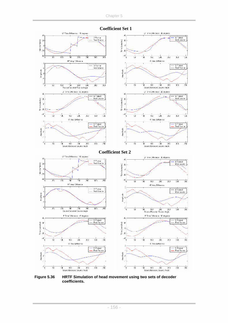
Chapter 5
Coefficient Set 1
Coefficient Set 2
Figure 5.36 HRTF Simulation of head movement using two sets of decoder
oefficients. c
- 156 -

Chapter 5
This is not the case for the 2nd set of coefficients and it can be seen that as
al
The evidence gathered from the HRTF analysis of the decoders’ performance
under head movement suggests that, as far as the low frequency velocity
vector is concerned, more information is needed to design a decoder that is
both stable under head rotation and has accurate image localisation.
However, as the velocity vector is used as an approximation to the interaural
time difference, it is now possible to alter the Tabu search algorithm described
in section 5.3.4 to ignore the velocity vector and deal directly with the
interaural time difference present for encoded sources around the unit circle.
This, on its own, may lead to potential performance increases as the
interaural time difference for a listener looking straight ahead can be mapped
more accurately using HRTF data, when compared to the velocity vector
theory. Also, head rotations can be simulated as shown above, and these
results taken into account when evaluating the fitness of a particular decoder.
ain
the same (decoder still has same number of coefficients etc.) but the
algorithm that supplies the Tabu search with its fitness coefficient must be
altered to take advantage of this new research.
the head is rotated, the virtual source’s time difference stays at approximately
0 samples difference. This means that when the head is rotated, the virtu
sound source will track with the listener, potentially making the resulting
sound field confusing and unstable.
5.3.6 HRTF Decoding Technique – Low Frequency
So, as is immediately apparent, the actual Tabu search algorithm will rem
∑ ∑= = ⎟
⎟⎟
⎠
⎞
⎜⎜⎜
⎝
⎛
⎟⎟⎠
⎞⎜⎜⎝
⎛
∂−
∂=
12
0
360
0
2
13m k
kdec
kref dd
Fitnessωφ
ωφ
(5.10)
φ=Average Phase Response (0-700Hz
k = Source angle
)
ω=Frequency
m=Head Rotation number.
- 157 -

Chapter 5
The fitness is now calculated using Equation (5.10) and then combined with
e pressure level (volume) fitness given in Equation (5.8) using the root
head
th
mean square value. Again, the closer this fitness value is to 0, the better the
performance of the decoder coefficients. In order to take into account
movement, this equation is evaluated using speaker rotations from 00 to 600 in
50 increments, and then the average fitness is taken.
0 50 100 150 200 250 300 350 400-40
-20
0
20
40LF Time Difference : 0 degrees
G FormatReal Source
0 50 100 150 200 250 300 350 400-40
-20
0
20
40LF Time Difference : 0 degrees
G FormatReal Source
0 50 100 150 200 250 300 350 400
-40
-20
0
20
40LF Time Difference : 30 degrees
G FormatReal Source
0 50 100 150 200 250 300 350 400-40
-20
0
20
40LF Time Difference : 30 degrees
G FormatReal Source
0 50 100 150 200 250 300 350 400-40
-20
0
20
40LF Time Difference : 60 degrees
G FormatReal Source
0 50 100 150 200 250 300 350 400-40
-20
0
20
40LF Time Difference : 60 degrees
G FormatReal Source
Figure 5.37 Comparison between best velocity vector (top) and a HRTF set of
coefficients (bottom).
Figure 5.38 Polar and velocity vector analysis of decoder derived from HRTF data.
In terms of the low frequency decoders that this technique produces, there is
a very high correlation between this HRTF method and the previous velocity
- 158 -

Chapter 5
vector analysis. That is, a decoder calculated using HRTF data produces a
e to
een
So,
equency response is much more difficult to match to that of a real source,
and most decoders derived using the energy vector theory have a response to
head rotations very similar to those shown in Figure 5.36. However, as is
shown in the listening test later in this chapter, although decoders can be
designed using HRTF data directly, taking head rotations into account, this
er
ed using velocity and energy vectors can, clearly, still have a good
is just that it is not due to the Tabu search
algorithm striving for this behaviour. However, when utilising velocity/energy
vector optimisations, the head rotation parameter can still be used in order to
differentiate between decoders’ performance as many resulting decoders are
possible.
good velocity vector plot as shown in Figure 5.38.
However, it can be seen that, in order to maintain the image stability du
head rotations, a compromise is needed between the accuracy of the
decoder’s localisation (according to the velocity vector) and its image stability
under head rotations. To see if this is actually the case Figure 5.37 shows the
HRTF analysis of the best velocity vector decoder (as used in Figure 5.36)
and a set of decoder coefficients derived using HRTF data. It can be s
that the resulting plots are almost identical for each reproduced angle and
degree of head rotation (00,300 and 600 in this case). The HRTF derived set
seems to actually have a better fit than the velocity vector analysis suggests,
and a slightly better fit than the original velocity vector decoder (which was
found to be the best of several found using the velocity vector technique).
as the decoder is now calculated taking head rotation into account, every
decoder now produced using this technique (as there are, again, multiple
solutions) will have an analytical performance similar to that shown in Figure
5.37.
5.3.7 HRTF Decoding Technique – High Frequency
As already stated (and as can be seen in Figure 5.36), the decoder’s high
fr
will not necessarily result in decoders that perform better under head rotations
than when designing a decoder using the energy vector analysis. It decod
design
response to head rotations, it
- 159 -

Chapter 5
The algorithm used to calculate the fitness parameter for the higher frequency
to be of a slightly different nature than that of the low
that
f
the
the
nder head rotation with the same priority as looking straight ahead,
ossibly resulting in a decoder that performs best when looking 300 to the left,
straight ahead, and so a weighting term
mu localisation fitness parameter is
giv that performed best
s
oor,
t the
hen compared to a centrally facing listener).
decoder actually needs
frequency system. This is due to the fact that after analysing the high
frequency lateralisation cues of many optimum decoders (optimum, in
they were optimised using the energy/velocity vector methods, or using purely
front facing HRTF optimisation) it was found that, due to the non-uniformity o
the speaker layout, high frequency head turning is more catastrophic for
amplitude cue when compared to the low frequency phase cue. If the
average fitness were used then the Tabu search would treat optimising
response u
p
for example. It makes more sense to have priority given to the decoder’s
output when the listener is facing
st be used. The equation used for the
en in Equation (5.11). This resulted in HRTF decoders
when the listener is facing straight ahead, as if the weighting parameter wa
not used, the Tabu search algorithm would converge on decoders with a p
analytical, performance (i.e. the fitness function did not truly represen
fitness of the decoder as a small increase in fitness when facing off-centre
made more of a difference w
( )∑=
=Fitness
(5.11)
f=average magnitude response between 700-3000Hz of a real source (ref) at
k0 from ce e at k0 from centre
−0
)()(k
decref kfkf 360
2
ntr front, and a decoded source (dec) located
front.
k=source angle (in degrees).
- 160 -

Chapter 5
5.3.8 Listening Test
5.3.8.1 Introduction
eters
y the work further now that a
technique mbisonic decoders has been made
available.
1. Dry
2. A p - nt space.
Each one
testing for one attribute more than another. As an example, if the recent
estionnaire:
a. Subjective room size – very big to small
d. Ensemble width – wide to narrow
bad,
ning to pre-
uggested by Berg & Rumsey, 2001,
could be envelopment, presence and naturalness). This type of material is
hard to s ng the
tested system to achieve. For example, accurate scene-capture and ‘best
In order to try and quantify any improvement that can be attributed to the
optimisation techniques described above, listening tests are needed.
Although the main body of this report concentrates on the numerical analysis
and optimisation of Ambisonic decoders using the lateralisation param
and velocity and energy vectors, a number of small listening tests were
developed in the hope that others will carr
for optimising irregular A
When designing the listening tests, there are two main types of material that
can be presented to the listener:
, synthetically panned material
re recorded real event in a reverbera
of these extremes will result in a test that will be more suited to
Project Verdi test is observed (Multi Media Projekt Verdi, 2002), two
recordings in a reverberant space were used, with the following attributes
tested in the qu
b. Localisation accuracy – very good, precise to bad
c. Ensemble depth – deep to flat
e. Realism of the spatial reproduction – very good, natural to
unnatural
f. Personal preference – very good to bad.
These are typical of the types of spatial attributes tested when liste
recorded material (although others, s
te t, in some ways, as it does depend on what you are expecti
- 161 -
Chapter 5
sounding’ are not necessarily synonymous; ultimately, the personal
preference parameter may be of greater importance.
Conversely, the most common form of test carried out on
a dry, synthetically
panne o
source (ag sen, 1991 and
Ordun t
attributes can often lead to a fuller picture of what a particular system is
achiev
i. Source stability (with respect to head movement).
d system, the ideals of the system
ch:
orientation.
ce of any multi-speaker
system the
above poi
As far t
direct c lly panned, dry
perceived source position.
• Increased image stability with respect to head turning.
Other effects of the optimisation may be (again, with regard to an
Ambisonically panned, dry source):
• Change in perceived image width/focus.
• Timbral alteration due to differences between low and high
frequency decoders
d s urce is that of simple recognition of the angular placement of that
ain, see Moller et al., 1999, Kahana et al., 1997, Niel
a e al., 1995 as typical examples). However, evaluating other
ing. Such attributes could include:
g. Source width/focus
h. Source distance
When it comes to testing a surround soun
are easier to decide upon. The best case scenario would be a system whi
• Has small image width/good image focus
• Reproduces distance accurately
• Reproduces sources in a fixed position, regardless of listener
Also, not mentioned at this point is that the performan
in an off-centre position can also be assessed using any/all of
nts.
as he optimisations of the Ambisonic decoder are concerned, the
onsequences should be (with regard to an Ambisonica
source):
• Increased accuracy/matching of encoded source position to
- 162 -

Chapter 5
All of the above would also be true when listening to pre-recorded,
reverberant material, with potential increase in accuracy and coherency of the
lower order, lateralisation cues, resulting in improvements to the higher order
spatial properties of the reproduced audio environments:
• Envelopment should be increased, that is, the sense of being in a
real place, and not listening to an array of speakers.
• Spaciousness should more closely resemble that of the actual
event.
.
ssor (SoundField Ltd.,
n.d. a).
• Two decoders optimised using the energy and velocity vector.
• Two decoders optimised using HRTF data directly
An analysis of these decoders will now follow, using both the energy and
velocity vector and the HRTF decomposition methods described above.
• Depth perception should be more accurate.
To this end, in order to subjectively test these decoders, questions based
around these attributes should be designed.
5.3.8.2 Decoders Chosen for Testing
A small sample listening test was carried out to give an insight into which
specific decoders worked best, and also to observe any common features
with Ambisonic decoders designed for use with an ITU 5 speaker array in
order to influence further listening tests to be carried out after this research
Five decoders were chosen for this test comprising:
• One decoder using the default settings of the commercially
available SoundField SP451 Surround Proce
- 163 -

Chapter 5
Figure 5.39 Decoder 1 – SP451 Default Settings
Figure 5.39 shows the default settings of the commercially available SP451
Surround Processor unit. This decoder is frequency independent (i.e. both
high and low frequency decoders are the same), with all the virtual
microphone polar patterns being of type cardioid. This leads to various
problems when the decoder is viewed using energy and velocity vectors, with
the resultant lengths of the vectors being suboptimal, and all of the source
positions being shifted forwards (i.e. a source that should be at 450 will be
reproduced closer to around 200 when decoded). However, when the
resulting HRTF analysis is observed, the high frequency amplitude differences
are a surprisingly good match to that of an actual source, with the low
frequency time difference showing the greatest error.
- 164 -

Chapter 5
Figure 5.40 Decoder 2 – HRTF Optimised Decoder
Figure 5.41 Decoder 3 – HRTF Optimised Decoder
Figure 5.40 and Figure 5.41 show two examples of decoders optimised using
HRTF data directly. It can be seen that these two decoders have produced
similar results when looked at using the HRTF data directly and when using
the velocity and energy vector analysis, although the virtual polar patterns for
both high and low frequency decoders are quite different. Also, the two types
of analysis show good agreement as to the angular distortion introduced by
Decoder 3, with frontal sources not producing enough level difference
between the ears, and so pushing sources towards the front of the speaker
- 165 -

Chapter 5
array. Decoder 2 has a much better encoded/decoded source position
agreement which is, again, shown in both the HRTF and velocity/energy
vector analysis at high frequencies, with very similar performance, again using
both forms of analysis, at low frequencies.
Figure 5.42 and Figure 5.43 show the two decoders that were designed using
the velocity and energy vector theories. One thing to note, firstly, is that these
decoders were optimised using rear speaker positions of +/- 1150 instead of
listening
test was carried out, but this is why the low frequency velocity vector match is
not as good as those shown in Section 5.3.4. Again, both of these decoders
have quite different low frequency virtual microphone polar responses, but
have near identical velocity vector responses. However, if the HRTF data is
looked at, it can be seen that Decoder 4’s low frequency phase differences
can be seen to have significant errors around the rear of decoder’s response,
showing a ‘flipping’ of the image cues at source positions of 1600 and 2000.
The high frequency decodes were designed using slightly different criterion,
with the angular accuracy of Decoder 4’s energy vector reproduced angle
being given a slightly smaller weighting, resulting in a higher error in the
reproduction angle for the rear of the decoder, but with the localisation quality
(vector length) benefiting from this approach.
the usual +/- 1100. Unfortunately this was not noticed until after the
- 166 -

Chapter 5
Figure 5.42 Decoder 4 – Velocity and Energy Vector Optimised Decoder
Figure 5.43 Decoder 5 - Velocity and Energy Vector Optimised Decoder
- 167 -

Chapter 5
Figure 5.44 Comparison of low frequency phase and high frequency amplitude
differences between the ears of a centrally seated listener using the 5 Ambisonic decoders detailed above.
Although the HRTF analysis of the various decoders has been shown, no
mention has yet been made of the performance of each decoder, numerically,
with respect to head turning. Figure 5.44 shows each decoder’s performance,
from 00 (facin een that all optimised
when compared to a real source, with respect to a listener turning their head
g straight ahead) to 500. It can clearly be s
- 168 -
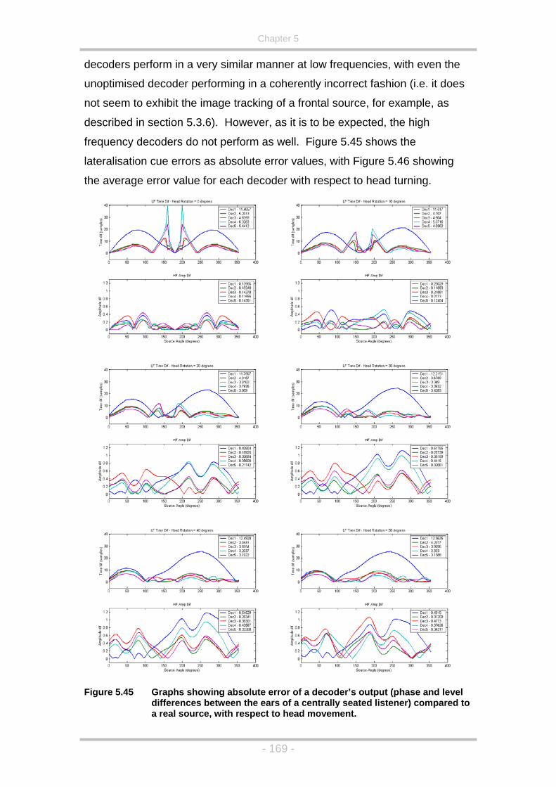
Chapter 5
decoders perform in a very similar manner at low frequencies, with even the
unoptimised decoder performing in a coherently incorrect fashion (i.e. it does
not seem to exhibit the image tracking of a frontal source, for example, as
described in section 5.3.6). However, as it is to be expected, the high
frequency decoders do not perform as well. Figure 5.45 shows the
lateralisation cue errors as absolute error values, with Figure 5.46 showing
the average error value for each decoder with respect to head turning.
Figure 5.45 Graphs showing absolute error of a decoder’s output (phase and level
differences between the ears of a centrally seated listener) compared a real source, with respect to head movement.
to
- 169 -

Chapter 5
Figure 5.46 Graph Showing the Average Time and Amplitude Difference Error with
Respect to A Centrally Seated Listener’s Head Orientation.
Figure 5.46 shows, in a very simplified manner, how each decoder will
perform. Using this graph as an indicator for overall performance, it can be
seen that, as already mentioned, all of the decoders perform almost equally
as well with respect to low frequency phase cues, with Decoder 1 having, by
far the worst error, but, as already mentioned, an error that stays reasonably
consistent with head turning. However, it is the high frequency plots that give
more insight into the performance of any decoder, as it is the high frequency
decoder that is most difficult to optimise, using either energy vector of HRTF
techniques. Performing best, here, is Decoder 2, which was designed with
(although, only up to 30 degrees). However, the head turning as a parameter
decoder with the next best high frequency error weighting is Decoder 5 which
is a decoder designed using the energy and velocity vector principles. It must
also be noted that, although the decoders all seem to perform similarly (under
numerical analysis), looking at the low frequency errors it can be seen that,
again, decoder 5 performs very well (best, in fact), but decoder 2 at low
frequencies is one of the worst performing decoders (ignoring Decoder 1).
Although there are four optimised decoders tested, each low frequency and
high frequency decoder was designed separately. No criteria has yet been
- 170 -

Chapter 5
set for deciding which low frequency decoders will complement particul
frequency decoders and so the decoders have been paired randomly
(although always grouped with a decoder that was optimised in the same wa
that is, using either HRTF or velocity/energy vector methods).
5.3.8.3
ar high
y,
Listening Test Methodology
For the actual listening test, two separate testing methods were chosen:
• A listening test similar to that described in section 5.2, measuring
the accuracy of panned, mono sources in the decoded sound field.
• A test where users give a preference as to which decoder performs
best when auditioning reverberant, recorded material.
These two styles of testing are not designed to be all-encompassing, but have
produced interesting points for use in further testing methodologies.
Two sources were chosen for the listening tests to be carried out. The source
that was to be synthetically panned was dry, female speech which is often
used in such tests (for example, see Martin et al., 2001, Kahana et al., 1997,
Moller et al., 1999 and Neilsen, 1992) due to its wide frequency range, and
reasonably un-fatiguing sound (especially when compared to band-limited
noise and other such sources). For the test of a real recording where decoder
preference was to be given by a 60 second excerpt from a recording made by
the company, Serendipity (2000), of Rick Wakeman playing the piano in
Lincoln Cathedral. It is a very reverberant recording made by a company that
has had significant experience with the SoundField Microphone, particularly in
the effective placing of the microphone (something that can often be
overlooked when choosing recorded material).
For this small test, three listeners were used. All three were experienced
listeners that had taken part in multi-channel sound system listening tests
before. The first test had sources presented to them, six source positions per
decoder. The source positions were identical for each decoder, but played in
pseudo-random order. The listeners were asked to indicate in which
a
direction they thought the source was coming from and to give an indication of
source width. This was to be recorded on the sheet shown in Figure 5.47
- 171 -

Chapter 5
which showed the layout of speakers in the University’s Multi-Channel
Research Lab. In addition, to aid in the recording of source position, each
speaker in the lab had a label fixed on it with its angular position relative to
straight ahead. They were asked to draw the size of the source, as this
method has proved to be more intuitive in these situations (Mason et al.,
2000).
Figure 5.47 Sheet given to listening test candidates to indicate direction and size of
sound source.
The user interface for controlling the listening test was constructed in Matlab,
which called Simulink models that encoded and decoded the mono sources in
- 172 -

Chapter 5
real-time, taking in a direction parameter that had been pre-entered. A screen
shot of this user interface is shown in Figure 5.48.
Figure 5.48 Screenshot of Matlab Listening Test GUI.
The listening test results showed reas
ifferent decoders when tested using the synthetically panned source, and
ts
ow
here
5.3.8.4 Listening Test Results
onably subtle differences between the
d
much more obvious differences when listening to a more complex, recorded,
sound field.
Figure 5.49 shows the results for the three listeners. The square data poin
represent the recorded source position with the error bars, above and bel
these positions showing the recorded source size for each decoder. It is
difficult to analyse these graphs directly, but it can be seen that all of the
decoders seem to perform reasonably well in this test with no image flipping
becoming apparent, although two sources were recorded as coming from
more than one location, subject 1 – decoder 4 and subject 3 – decoder 1.
Interestingly these were both at source position 2250, which is the area w
the decoders will all perform at their worst (i.e. at the rear of the sound field).
- 173 -

Chapter 5
Figure 5.49 Graphs showing the results of the panned source part of the listening
test for each subject. ‘Actual’ shows the correct position, D1 – D5 represent decoders 1 – 5.
In order to compare these results
error and i
expected, the image source’s graphical depi
subject (Mason
image size tual
source positions in order to record some
each listener, but this was
result is that decoder one seems to perfo
each subject (i.e. high mean error value)
other results, however, are slightly more
proposed in section 5.3.8.2 that de ted to
turning and the average localisation
results of subjects 2 and 3 are observed.
more equally, the average absolute angle
mage size can be seen for each subject in Figure 5.50. As is to be
ction of size is different for each
et al., 2000), with subject one generally recording smaller
s than subjects 2 & 3. It would be reasonable to insert ac
form of ‘calibration’ size source for
not attempted in this small test. Another obvious
rm worst, subjectively, according to
. This was an expected result. The
varied from listener to listener. It was
coders 5 and 2 would be expec
perform best, taking into account head
error this would produce. However, only subject 1 seemed to agree with this
statement in its entirety. Decoder 5 did perform consistently well throughout
this phase of the test, but decoder 2 performed less favourably when the
- 174 -

Chapter 5
Figure 5.50 Graph showing mean absolute perceived localisation error with mea
source size, against decoder number.
There are a number of potential reasons for this:
• Subject 1 was the most experienced listener in thi
n
s test, and may
give the most correct, or predictable results.
be
nging the way they are grading the results (or learning how to
cts 2 and 3
•
ious
Figure 5 e for each
decoder. It must be noted that, as the image size for each subject has not
been no der)
• Decoder 5 is located at the end of the test, and the subjects may
cha
interpret them better) as the test continues. This may be
corroborated by the general downwards slope that subje
show in their average error results.
The low and high frequency decoders interact in some more
complex, non-linear way than has been simulated in the prev
analysis of the decoders (i.e. the low and high frequency decoders
should not be designed and analysed in isolation).
.51 shows the average absolute error and image siz
rmalised, the image size ratios of subject 1 (from decoder to deco
- 175 -

Chapter 5
will have verage
absolute
less of an effect than that of subjects 2 and 3. However, the a
localisation will not be affected.
Figure 5.51 Graph showing the mean, absolute, localisation error per decoder
taking all three subjects
into account.
Figure 5.51 shows that, overall it is decoder 5 that seems to perform best in
ownwards lope, starting with decoder 1, being clearly
evident in this figure. Also evident is the already mentioned, relatively equal
performance of all of the optimised decoders, with an average error between
100 and 160 compared to decoder 1’s average error of 210.
sted below:
n
rce,
distance as the speakers, whereas rear images were perceived
this test, with the d s
Other non-recorded observations were also evident from this test, and are
li
• Head movement helped greatly in the localisation of sources in this
experiment, and were used extensively by each listener.
• It was noted that although front and side sources were generally very
stable (an impressive result by itself, when compared to amplitude
panned material or the observations of Craven’s higher order
decoder (Craven, 2003)), rear images only performed correctly whe
facing forwards. That is, when the subject turned to face the sou
the two rear speakers were perceivable as sources. In these cases
all subjects recorded the position facing forwards.
• Front and side images were generally perceived at the same
- 176 -

Chapter 5
m
s
The rear i
rear imag r
methods all point to rear images performing less well. However, the fact that
rear im e
impressive result.
The 2nd pa of
a piano re
decode s ut
which versions they wished to hear again. This was continued until a
preference was given as to which decoder they thought performed best. The
uch closer to the head, almost on a line joining the two rear
peakers of the ITU speaker array.
mage problems are not wholly unexpected as it can be seen that
es due to head turning and analysis using the velocity/energy vecto
ag s can be formed at all, with a speaker hole of 1400, is still an
rt of the listening test was the auditioning of a 60 second except
cording made in Lincoln Cathedral. Each listener heard each
r’ representation of this piece once and was then invited to call o
results of this test were as follows:
Preference Subject 1 Subject 2 Subject 3
Best 1st 3 3 3
2nd 5 2 5
3rd 2 5 4
4th 4 4 2
Worst 5th 1 1 1 Table 5.1 Table showing decoder preference when listening to a reverberant, pre
recorded piece of music.
The results showed a clear trend, showing that decoder 1 was by far the wor
of the five decoders, but with decoder 3 clearly being preferred by all three
listeners. This decoder, although not performing as well under head-turning
analysis, is the only optimised decoder to have significant shifting of sources
towards the front, when looking at Figure 5.41, as s
-
st
hown in both the energy
vector d as just
using the
perceived more
subjec e
subjects d
an HRTF analysis at high frequencies. This is not the same
forward dominance control as decoder 3 maintains the overall
volume equally from all directions. This, therefore, could be a
tiv , artistic artefact of this decoder, although comments from the
id indicate some of the reasons for choosing this decoder:
- 177 -

Chapter 5
• Subjects 1 & 2 commented that decoders 5 & 2 (which they rated
2nd and 3rd, and 3rd and 2nd respectively) were very similar in
3
this.
e
• was very front heavy, with an obvious
cen -
head’ at the sweet spot, when compared to the other decoders.
• Sub
decoder 3, had a very ‘tangible’ quality to it.
This o
Ambison ce
of decod
expected, although the differences between the decoders, overall, was more
subtl h
more sta
performa
part of th
made to try and remove any bias from the results:
may eliminate the general downward sloping of
each
performance, both with a slightly ‘oppressive’ sweet spot. This,
interestingly, disappeared when auditioned off-centre. Decoder
did not suffer from
• Subject 1 mentioned that decoder 4 had a very wide, more diffus
image.
All agreed that decoder 1
tre speaker, and 2 subjects mentioned that it was almost ‘in
ject 1 commented that the Piano, when reproduced using
5.3.8.5 Listening Test Conclusions
The listening test, although only being presented to a very small number of
subjects, was a useful exercise, bringing to light a number of attributes that
should be researched further. The most obvious result was that the un-
optimised decoder, based on the standard settings of the commercially
available B-Format decoder, clearly performed less-well in both of the tests.
sh ws that both optimisation methods do improve the performance of
ic decoders for a five speaker irregular array. Also, the performan
er 5 in the first stage of the listening test (panned source) was also
e t an expected, and a much larger test base would be needed to gain
tistically significant results. However, the fact that the extremes of
nce were shown in this small test is a very encouraging result. If this
e test were to be carried out again a number of changes would be
• The order of presentation of the test decoders would be
randomised. This
the average localisation results observed in subjects 2 and 3.
• The test would be carried out over more than one day, testing
subject at least twice to try and measure what kind of variations
each one was likely to produce.
- 178 -

Chapter 5
• More source locations would be used so as to map more accur
the performance of each decoder.
ately
• Actual sources would be played at random, so that a ‘calibration’
• A distinction could be made between source stability and image
nning two separate tests (and allowing separate
ers
t
:
at can
e four optimised decoders
esting, especially as these were, analytically,
suggests that over-optimising for
f a
re
described by the listener and compared against later (i.e. actual source
source width is available to judge better the width parameter of
subject’s results.
location by ru
analyses on the results):
1. Where the subject is asked to face forwards at all times
(knowing they will move their head a little, still).
2. Where the subject is asked to face each source before
recording its position.
Interestingly, the decoder that was unanimously voted as the ‘best’ decoder
when listening to pre-recorded material was an unexpected result (however,
the decoder perceived as ‘worst’ was not) with the middle group of decod
needing a larger base of subjects in order to gather a statistically significan
result. Although this was a very simple test, with only one parameter, it did,
indirectly, reveal some valuable insight into the performance of the decoders
• Most listeners are often surprised by the amount of variation th
be achieved just by altering the decoder, with spaciousness and
envelopment being altered massively (especially when compared to
decoder 1).
• The sweet-spot problems with two of th
were particularly inter
the best performing decoders. This
a single position may, in fact, be detrimental to the performance o
decoder.
• The best sounding decoder may not be the one that is, necessarily,
the most accurate.
Testing the performance of a decoder using pre-recorded material is far mo
difficult to grade when compared to the first test. A number of different
recordings should be used and tests where the recording situation can be
- 179 -

Chapter 5
positions, size of room etc.) could be used to try to neutralise the artistic
aspect of the decoder’s performance, if necessary.
5.4 The Optimisation of Binaural and Transaural Surround Sound S .
5.4.1 Introduction
Bina duction techniques are based upon
e optimised using a similar
esised (and recorded)
inaural material is that the reproduction is normally perceived as filtered.
ct is experienced with the
If a 2 x 2 set of impulse responses are
inverted so as to create a pair of crosstalk cancellation filters, then the
frequency response of these filters will be perceived, both on and off-axis,
even though the theory states that this response is actually compensating for
a pinna filtering response. The most logical method of correcting these
artefacts is to use inverse filtering techniques.
.4.2 Inverse Filtering
esponse
e
of a
the
ystems
Both the ural and Transaural repro
HRTF technology and, for this reason, can b
approach. One of the main problems with synth
B
That is, the listener will not perceive the pinna filtering (and normally the
microphone and headphone filtering too) present in the recording as
transparent. Possible reasons for this could be that the pinna filtering on the
recording does not match the listener’s, or because no head tracking is used:
minute head movements can not be utilised to help lateralise the sound
source and so the frequency response heard is assumed to be that of the
source itself by the ear/brain system. A similar effe
use of crosstalk cancellation filters.
5
Inverse filtering (which has already been touched upon in Chapter 3) is a
subject that is very simple in principle, but takes a little more care and
attention in practice. Inverse filtering is the creation of a filter whose r
will completely equalise the response of the original signal. The general cas
is that of a filter that is created to force the response of a signal to that
target response and is analogous to re-arranging an equation where
answer is already known, where the value of a variable (in this case, a filter)
- 180 -

Chapter 5
needs to be found. The time domain representation of this problem is given
in Equation (5.12).
( ) ( ) ( )
( ) ( )( )nanunh
nunhna
=
=⊗
(5.12)
where: a(n) = original response.
u(n) = target response.
h(n) = inverse filter (to be found).
In Equation (5.12) ⊗ represents polynomial multiplication (convolution) and
the division represents polynomial division (deconvolution). A much more
efficient approach to this problem is to process all of the data in the frequency
domain using the Fast Fourier Transform algorithm. This then transforms the
at is, the
polynomial arithmetic into a much quicker point for point arithmetic (th
first value of ‘u’ is divided by the first value of ‘a’ and so on). These frequency
domain equations are shown in Equation (5.13).
( ) ( ) ( )
( ) ( )( )ωωω
ωωω
auh
uha
=
=×
(5.13
where: ω = angular frequency.
If we were to take a head related transfer function and find the inverse filter in
this way the filter shown in Figure 5.52 will be produced. There are a n
of artefacts that can be observed, but first it should be noted that the
magnitude response of the inverse filter already appears to be just that, the
inverse response (mirror image about the 0 dB mark), as given by the
equations above (an inverse filter can be thought of as inverting the
)
umber
agnitude and negating the phase as described in Gardner & Martin (1994)).
m
- 181 -

Chapter 5
Figure 5.52 Inverse filtering using the equation shown in Equation (5.13)
Unwanted audio artefacts can be clearly seen in the time domain
representation of the original and inverse signals convolved together
(theoretically they should produce a perfect unit pulse if the inversion has
been carried out successfully). Also, the inverse filter does not look complete
in that it does not have a definite start and end point as can be observed in
most filter impulses (this, on its own, however, is not necessarily an issue).
The problem seen in the time domain response of the two signals convolved
can be quantified if the frequency domain magnitude response is calculated at
a higher resolution as shown in Figure 5.53 (the frequency domain plot in
sing this hig shows the excessive ripple that has been
format to have a window applied.
Figure 5.52 was calculated with a length equal to that of the filter). Analysis
her resolutionu
introduced by this filter. This can be resolved, as in any other type of filter
design, using windowing techniques (Paterson-Stephens & Bateman, 2001).
However, the impulse response shown in Figure 5.52 is not yet in the correct
- 182 -

Chapter 5
Figure 5.53 Frequency response of the original and inverse filters using an 8192
point F.F.T..
An F.I.R. filter3 is basically a cyclic signal that will wrap around onto itself.
This means that when the inverse filter is calculated, the position of the filter
(in the impulse space) is not necessarily correct. For example, the envelope
of the filter created in Figure 5.52 is shown in Figure 5.54 along with the ideal
position of this filter.
Figure 5.54 Typical envelope of an inverse filter and the envelope of the filter shown
is this main impulse that dictates
in Figure 5.52.
It can be seen in Figure 5.54 that it is desirable for the main impulse to be in
the centre of the filter so as to maximise the number of samples given to pre
and post delay processing for the sound. It
3 Finite Impulse Response – a filter with a fixed length that is convolved (polynomial
multiplication) with a signal to apply the filter’s time and frequency response onto the signal.
- 183 -

Chapter 5
the overall time delay introduced by the filter. As the F.I.R. filter can be
treated as a continuous wrappable signal, the impulse response can be
repositioned by adding a delay to the response that is to be inverted, as
shown in Figure 5.54. To move the main impulse to the centre of the filter, a
delay of N/2 samples must be added, where N is the length of the target filter,
in samples. This technique also has the benefit of improving the frequency
response of the filter, as shown in Figure 5.55 (note that due to the extra
samples (zero padded) added to the shifted filter, both filters have been
calculated using 256 samples).
Figure 5.55 Two F.I.R. filters containing identical samples, but the left filter’s
envelope has been transformed.
It can now be seen that the frequency response of the filter has been
proved and much of the rippling has been eliminated. This results in a
reduction of the artefacts seen in the time domain version of the original and
inverse filters convolved (as shown in Figure 5.52, bottom left plot). This is
shown in Figure 5.56.
im
- 184 -

Chapter 5
Figure 5.56 The convolution of the original filter and its inverse (both transformed
and non-transformed versions from Figure 5.55).
Now that the filter is in the correct format, a window function can be applied to
smooth the response still further, and help reduce these time and frequency
a
mited filter s able response without using the
regularisation parameter described in Chapter 3. The only method of
improving this further is to create a longer response using zero-padding of the
filters used to calculate the inverse. However, the resulting size of the HRTF
filters must be taken into account as convolution of the inverse filter and the
original HRTF filter will cause its response to increase in size. If the HRTF
filter is of length ‘a’ and the inverse filter is of length ‘b’ then the resulting filter
will be of a length ‘a+b-1’, and the longer the filter, the more processing power
will be needed for it’s implementation. The differences between using a
shown in
domain artefacts. The windowed response is shown in Figure 5.57. Using
ize, this is the best realisli
windowed 256-point filter and a windowed 1024-point filter are
Figure 5.58.
- 185 -
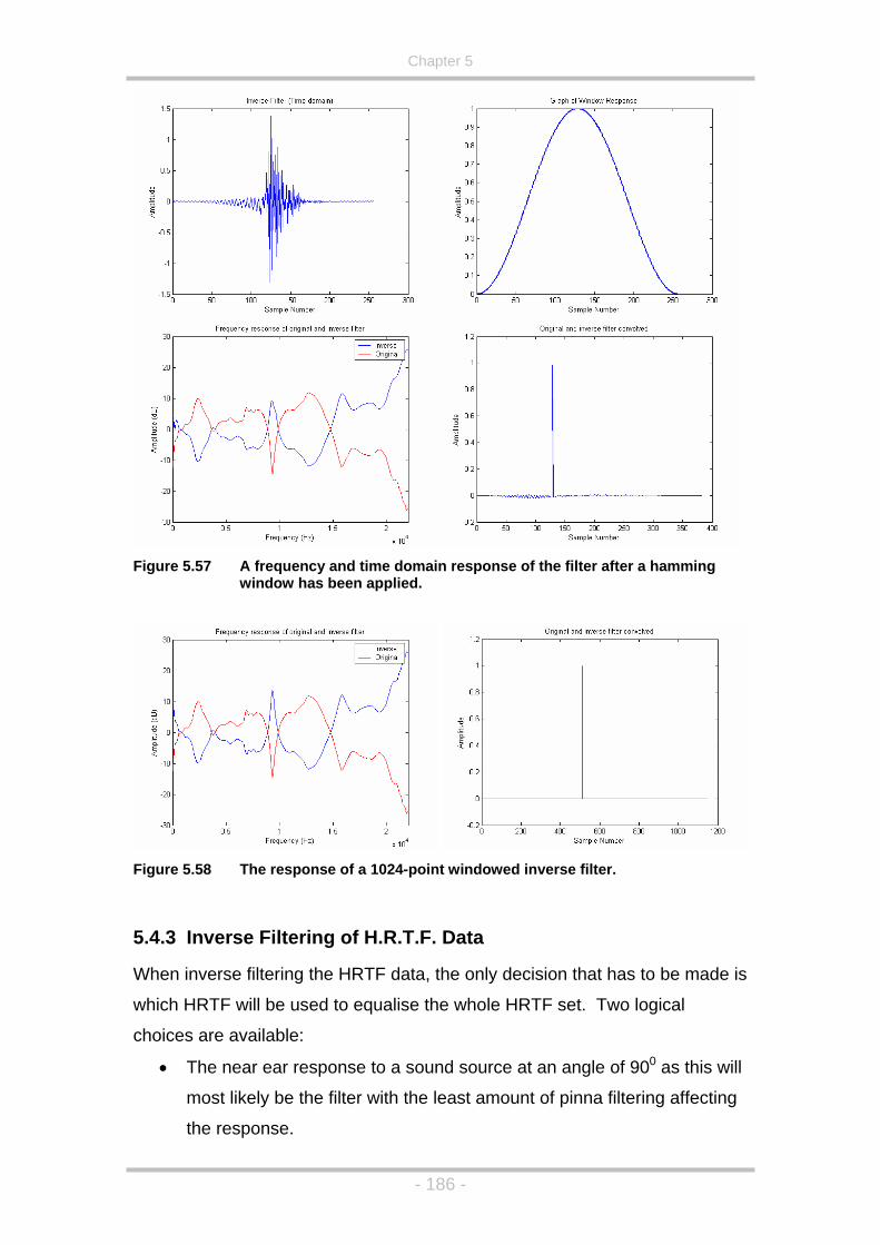
Chapter 5
Figure 5.57 A frequency and time domain response of the filter after a hamming
window has been applied.
Figure 5.58 The response of a 1024-point windowed inverse filter.
rs
hen inverse ecision that has to be made is
most likely be the filter with the least amount of pinna filtering affecting
the response.
5.4.3 Inve e Filtering of H.R.T.F. Data
filtering the HRTF data, the only dW
which HRTF will be used to equalise the whole HRTF set. Two logical
choices are available:
• The near ear response to a sound source at an angle of 900 as this will
- 186 -

Chapter 5
• The ear’s response to sound directly in front of the listener so that
when the sound is positioned at 00, the H.R.T.F. responses at the ears
are identical and flat.
The 1024-point inverse filters for both of these methods are shown in Figure
5.59. Looking at this figure it can be seen that, in reality, the 00 HRTF is far
more ill-conditioned to the inversion process when compared to the 900
response. Some wrapping of the resulting filter can be seen for the 00
response indicating that a longer filter length is desirable. This is to be
expected because of the reason stated above (the 900 angle has less
head/pinna filtering associated with it) and so it is best to use the 900, near
ear, HRTF as the reference response.
Figure 5.59 The 1024-point inverse filters using a 900 and a 00, near ear, HRTF
response as the signal to be inverted.
As an example, a set of H.R.T.F. data has been processed in this way using
an inverse filter size of 769-points (so that the convolution of the original with
this inverse filter will be equal to 1024-points). Figure 5.60 shows a number of
- 187 -

Chapter 5
the H.R.T.F. impulses in the time and frequency domain so a comparison of
them can be made both before and after inverse filtering.
Before Inverse Filtering After Inverse Filtering
Figure 5.60 Comparison of a HRTF data set (near ea
and after (left hand side) inverse filteringr only) before (right hand side) has been applied, using the
900, near ear, response as the reference.
Figure 5.60 shows that although both sets of HRTFs still have a pinna filtering
effect, the inverse filtered set have a larger bandwidth, in that extreme low
and high frequency components of the impulse responses contain more
energy, and contain peaks and troughs in the frequency response that are no
larger the originals (for example, the 135 degree frequency response plots
both have a notch no lower than around -27 dB). These inverse filtered
HRTFs are perceived to be of a better fidelity than that of the originals (which
rse filtering of
e source’s response that was used to record the HRTF data in the first place
have this response due, in some part, to the non-optimum inve
th
(Gardner & Martin, 1994)). It can also be seen that due to the nature of these
new inverse filtered HRTFs, they could also be windowed and shrunk if
- 188 -

Chapter 5
smaller responses were needed due to processing constraints thanks to the
roughly equal amount of pre and post delay filtering (i.e. the highest amplitude
parts of the filter are at the middle sample position).
5.4.4 Inverse Filtering of H.R.T.F. Data to Improve Crosstalk Cancellation Filters.
As mentioned at the start section 5.4, one of the problems of the crosstalk
cancellation system is that very noticeable colouration of the reproduced
sound can occur, both due to the crosstalk cancellation itself, and due to the
response of the individual parts of the system (usually speaker to near ear,
r
rosstalk cancellation in the free field and crosstalk cancellation using HRTF
cies. For this
reason, it is desirable to minimise any potential ill-conditioning due to the
response of the individual components of the system prior to the 2 x 2 matrix
inversion process, thus resulting in the least amount of regularisation needed
in order to create a useable set of filters. In this way, the inverse technique
described in section 5.4.2 will be utilised in much the same way. For
example, the system shown in Figure 5.61 will be used as a basis for the
creation of a pair of crosstalk cancellation filters.
and speake to far ear responses). This is why there is a difference between
c
data. However, as discussed in Chapter 3, system inversion using frequency-
dependent regularisation can be used to compensate for this, at the expense
of the accuracy of the crosstalk cancellation at these frequen
100
Figure 5.61 System to be matrix inverted.
This is a typical arrangement for a crosstalk cancellation system, and is based
on a pair of speakers placed at +/- 50 in front of the listener. Using the HRTF
- 189 -

Chapter 5
set from M.I.T. (Gardner & Martin, 1994) this will give the responses for the
near and far ears (assuming symmetry) as shown in Figure 5.61.
Figure 5.62 HRTF responses for the ipsilateral and contralateral ear responses to
the system shown in Figure 5.61.
If a set of crosstalk cancellation filters are constructed from these two i
responses, using the techniques described in Chapter 3, then the responses
shown in Figure 5.63 are obtained (using no regularisation).
mpulse
Figure 5.63 Crosstalk cancellation filters derived using the near and far ear
responses from Figure 5.62.
It can be seen, from Figure 5.63, that the expected peaks are present. That
is, a peak at very low frequencies due, mainly, to the close angular proximity
of the speakers and the peaks at around 8 kHz and high frequencies, which
appear to be due to the inversion of the responses of the near and far ear
HRTFs (as seen in Figure 5.62). When this crosstalk cancelled system is
auditioned, not only is a very coloured sound perceived off-axis, but a non-flat
is. This is also coupled with a
the amplifier and speakers have to
reproduce such a large difference in frequency amplitudes. These are mainly
frequency response is also perceived on-ax
large loss in useable dynamic range as
- 190 -
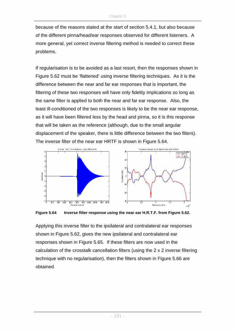
Chapter 5
because of the reasons stated at the start of section 5.4.1, but also because
of the different pinna/head/ear responses observed for different listeners. A
more general, yet correct inverse filtering method is needed to correct these
problems.
If regularisation is to be avoided as a last resort, then the responses shown in
Figure 5.62 must be ‘flattened’ using inverse filtering techniques. As it is the
difference between the near and far ear responses that is important, the
s
e near and far ear response. Also, the
least ill-conditioned of the two responses is likely to be the near ear response,
as it will have been filtered less by the head and pinna, so it is this response
that will be taken as the reference (although, due to the small angular
displacement of the speaker, there is little difference between the two filters).
The inverse filter of the near ear HRTF is shown in Figure 5.64.
filtering of these two responses will have only fidelity implications so long a
the same filter is applied to both th
Fig
Applyin
shown
responses shown in Figure 5.65. If
cal a ring
techniq
obtain
ure 5.64 Inverse filter response using the near ear H.R.T.F. from Figure 5.62.
g this inverse filter to the ipsilateral and contralateral ear responses
in Figure 5.62, gives the new ipsilateral and contralateral ear
these filters are now used in the
cul tion of the crosstalk cancellation filters (using the 2 x 2 inverse filte
ue with no regularisation), then the filters shown in Figure 5.66 are
ed.
- 191 -
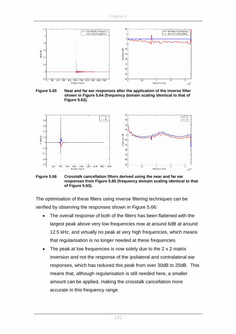
Chapter 5
5.65 Near and far ear responses after the application of the inverse filter
shown in Figure 5.64 (frequency domain scaling identical to that of Figure 5.62).
Figure
Figure 5.66 Crosstalk cancellation filters derived using the near and far ear
responses from Figure 5.65 (frequency domain scaling identical to thatof Figure 5.63).
The optimisation of these filters using inverse filtering techniques can be
verified by observing the responses shown in Figure 5.66:
• The overall response of both of the filters has been
flattened with the
largest peak above very low frequencies now at around 6dB at around
12.5 kHz, and virtually no peak at very high frequencies, which means
that regularisation is no longer needed at these frequencies.
• The peak at low frequencies is now solely due to the 2 x 2 matrix
inversion and not the response of the ipsilateral and contralateral ear
responses, which has reduced this peak from over 30dB to 20dB. This
means that, although regularisation is still needed here, a smaller
amount can be applied, making the crosstalk cancellation more
accurate in this frequency range.
- 192 -

Chapter 5
• The flattening of the filter responses causes the on-axis response to be
perceived as much flatter (un-filtered) than before.
• The flattening of the filter responses also has the added effect of
making off-axis listening seem far less filtered.
• The crosstalk cancellation filters are actually smaller in length than the
originals shown in Figure 5.63, even though the contralateral and
ipsilateral ear responses used to calculate them were much larger than
the originals shown in Figure 5.62. This is due to the fact the new near
and fa ch less ill-conditioned for inversion (the filters
do not have to ‘work as hard’ to achieve crosstalk cancellation).
, and
ng of the system. If the
filter representing ‘h1’ is used as a reference, then another inverse filter can
be created by inverting the response of ‘h1’. If this inverse filter is convolved
with both h1 and h2 then the h1 filter will, in theory, become the unit impulse,
and h2 will then be a filter representing the difference between h1 and h2.
These filters are shown in Figure 5.67, and Figure 5.68.
r responses are mu
These new crosstalk cancellation filters, although much better than filters
created using the raw HRTF data, still need to use some regularisation
still sound a little bass heavy. However, at this point, it is still possible to take
the inverse filtering technique a step further. As always, it is the difference
between the two ears that is important, especially as the pinna used in the
HRTF data is not likely to be the same as that of the listener. So, using
inverse filtering, it is possible to design crosstalk cancellation filters that
require no regularisation to correct for the conditioni
Figure 5.67 Filter representing inverse of h1, in both the time and frequency
domain.
- 193 -

Chapter 5
Figure 5.68 Crosstalk cancellation filters after convolution with the inverse filter
shown in figure 5.51
It can be seen from Figure 5.68 above that h1 has a flat frequency response
and h2 now has very little energy over the 0dB point meaning that the system
needs no regularisation. These new, double inverted, filters are also
perceived as performing much better than the previous crosstalk cancellation
filters, with a less muffled sound and clearer imaging. One other highly useful
feature of these new filters is that h1 can be approximated by a unit impulse
(as this is what h1 should be, theoretically, anyway) which cuts the amount of
FIR filtering in the system by a half, replacing the h1 filters with a simple delay
line, as shown in the block diagram in Figure 5.69.
re
esponse when compared to the single inverted case (which is perceived
as having a raised bass response anyway). For example, if we inject an
impulse into the block diagram shown in Figure 5.69 (but replacing the delay
Figure 5.69 The optimised crosstalk cancellation system
However, these double inverted filters do mean that when the speakers a
positioned close to each other, the response can be perceived as lacking in
bass r
Left Ear Signal
Right Ear Signal
H2 Filter
H2 Filter
+ +
+ +
Left Speaker
Right Speaker
Z-m
Z-m
where m is the delay line length
- 194 -

Chapter 5
line with the filters again) and compare the results that will arrive at the ear of
a listener (although it should be noted that the analysis is using the non-
optimum frequency response of the MIT HRTF data), the results shown in
Figure 5.70 can be seen (note that the speakers in the University of Derby’s
Multi-channel research laboratory are actually placed at +/- 30, and so filters
for this speaker arrangement is shown in Figure 5.70).
Fig
,
is, again, is not suggested in this plot. It is also, 0
ure 5.70 Left Ear (blue) and Right Ear (red) responses to a single impulse injected into the left channel of double and single inverted cross talkcancellation systems.
Both responses show a good degree of crosstalk cancellation, in the right ear
response, with the single inverted system seeming to perform slightly better.
The low frequency roll-off can also be noted in the left ear response of the
double inverted system. However, these quantitative results cannot
necessarily be taken at face value. For example, the single inverted system
(lower plot) is perceived as being bass heavy, although this is not shown in
these graphs as it is the non-optimum HRTF data used in this analysis. Also
the double inverted system is perceived as performing better at the higher
frequencies, although th
interesting to look at the same graphs for the +/- 30 case, as shown in Figure
5.71.
- 195 -

Chapter 5
Figure 5.71 Left Ear (blue) and Right Ear (red) responses to a single impulse
injected into the left channel of a crosstalk cancellation system.
This pl s
• The bass loss is no longer an issue. However this is to be expected as
wid
filte
• The cance t B
worse than th
This second poin
created in exactly th e. This means that the same
differences betw
filtering process is th
discrepancy that mu
that the further apar e
listener and the filters becomes important. This would explain why widening
the spe k
5.5 Conclusions
Optimisati s
chapter, w n concentrating on the optimisation of
e Ambisonics decoders.
ot hows two significant results:
ening the speaker span alleviates the bass boost in the original
rs which, in turn, means they do not need to be inverse filtered.
lla ion of the right ear signal is shown to be around 20d
at shown for the +/- 30 case.
t is interesting as the crosstalk cancellation filters have been
e same way as the +/-30 cas
een the filters will be retained. The only absolute in the
e response due to the pinna alone, and it is this
st be causing the problem. These two graphs suggest
t the speakers, the more the pinna matching between th
a ers degrades the localisation quality using this system.
on techniques have been described, analysed and discussed in thi
ith the main part of this sectio
th
- 196 -

Chapter 5
5.5.1 Ambisonic Optimisations Using Heuristic Search Methods
The main problem to be tackled in this section was the derivation of
Ambisonic decoders for irregular arrays, as, although Gerzon & Barton
had suggested some parameters to be used in the design of these decoders,
the solving of these
(1992)
equations was previously a lengthy and difficult process.
the analysis of the original work by Gerzon and Barton (1992 & 1998) it was
,
re
cy decoders’ perceived source position.
Variou e
solve thes
• istic search method, based on a Tabu search algorithm, has
r
s the three following benefits:
a
ts.
o This method solves all the parameters of the equations
rally
In
found that:
• Multiple values could be chosen that would satisfy these equations
analytically performing equally well.
• The original coefficients suggested by Gerzon & Barton (1992) we
actually non-ideal, with an oversight in the way in which the
equations were initially solved leading to a mismatch between the
low and high frequen
s n w methods have been devised and implemented in software to
e problems:
A heur
been developed, along with the fitness functions that need to be
satisfied in order to automatically generate decoders for irregula
speaker arrays. This method ha
o It automatically solves the non-linear simultaneous
equations in an optimal way.
o Changing the start position for the search will generate
different set of coefficien
simultaneously which corrects for the low and high
frequency decoder mismatch found in Gerzon & Barton’s
method (Gerzon & Barton 1992 and Gerzon & Barton
1998).
• An analysis technique based on the use of generic HRTF data has
been devised to help differentiate between Ambisonic decoders
designed using the above method, using head turning as an
additional parameter as phase and level differences will gene
be similar for each decoder.
- 197 -

Chapter 5
The tabu search method has also been shown to work well on the new
order decoder types, such as the one proposed by Craven (2003), which has
far more coefficients to optimise, demonstrating that the Tabu search
methodology is easily extendible to more unknowns (either a higher order, or
more speakers).
The HRTF analysis technique described above was als
higher
o used to validate the
riginal work by Gerzon & Barton (1992) which then led to the creation of a
sign
this
etween decoders designed
using the velocity/energy vector methods and HRTF methods are
ed at
n un-
ilable
be needed to gain statistically significant results,
all the optimised decoders performed well, with the expected decoder
performing best in the synthetically panned listening test. As expected, there
were no great differences between decoders designed using either
o
heuristic search program, with corresponding fitness functions, used to de
Ambisonic decoders for irregular arrays using the HRTF analysis technique
first proposed in Wiggins et al. (2001) taking into account head turning
directly, so reducing the number of decoders produced. The properties of
new technique are as follows:
• For a two-band decoder the correlation b
good.
• Using the HRTF technique a decoder could be designed using
more frequency bands, which is impossible using the previous
velocity/energy vector method.
• However, the HRTF decoder method is far more computationally
expensive and it does take the tabu search algorithm longer to
converge on an optimum result, but as this is an off-line process
anyway, this is not a major issue.
A small listening test was carried out using both synthetically panned material
and pre-recorded material in order to help steer future listening tests aim
optimised Ambisonic decoders. Although only three subjects were used, the
decoder that performed worst in both tests was unanimously seen as a
optimised decoder based on the default settings of a commercially ava
B-format decoder for the ITU irregular speaker array. However, although
many more subjects would
- 198 -

Chapter 5
optimisation method, as the two systems correlate well with respect to
coefficients and, in fact, slightly less optimal decoders seemed to perform well
cts.
seemed to
st
ng for the
ions (Gerzon & Barton, 1992 & 1998) to be solved correctly for
regular speaker arrangements (although the software concentrates on a
tep
irs (or 1 set
which could, potentially, lead to a control
ove h
performance around this spot. This may well be beneficial, not only to create
a ‘v u
listenin lly
speaking, giving a slightly uncomfort
directly in the sweet spot.
when recorded, reverberant material was auditioned by the test subje
Also, one reported observation was that the most optimal decoders
deliver a more pleasant listening experience slightly off-centre (when
compared to the same decoder in the sweet spot), which is an extremely
interesting result that needs to be investigated further.
In summary, the use of the Tabu search algorithm has resulted in a va
simplification of the process of designing Ambisonic decoders, allowi
Vienna equat
ir
typical five speaker horizontal arrangement). This has then been taken a s
further through the use of the HRTF data directly.
5.5.2 Further Work for Ambisonic Decoder Optimisation.
Now that the decoder design algorithm can directly use HRTF data the
obvious next step is to increase the number of frequency bands. When taking
this method to its extreme, this will mean that instead of using cross-over
filters, a W, X and Y filter will be created for each of the speaker pa
for the centre speaker). In this way it should be possible to maximise the
correctness of both the level and time differences simultaneously for many
frequency bands improving the performance of the decoder still further for a
centrally seated listener. The software could also be extended to take into
account off-centre listening positions
r t e sweet spot size, trading the performance at the centre, for the
ol me solution’, but to also circumvent the problems noticed in the
g test with respect to the more optimum decoders, analytica
able, obtrusive listening experience
- 199 -

Chapter 5
5.5
The us data has proved an
inv a
reprod quency response of the crosstalk
upper
frequencie HRTF data is present) it is still
advisable to use regularisation to stop the excessive boost of these
n the
he differences between the creation and analysis
RTF filters were kept constant, with only the monaural pinna filtering having
d
s.
filter, in
de the magnitude responses of the two filters using the desired
• Mix
and
.3 Binaural and Transaural Optimisations Using Inverse Filtering.
e of inverse filtering techniques on HRTF
alu ble tool in the optimisation of both Binaural and Transaural
uction. An improvement in the fre
cancellation filters has been demonstrated which is apparent both on and off
axis from the cancellation position. This reduces the need to use the
frequency dependant regularisation function; although at the extreme
s (where little energy in the
frequencies.
It has also been shown how moving the speakers closer together has the
effect of improving the analytical crosstalk cancellation figure betwee
ears of a listener in the sweet spot. This has to be a feature of the pinna
filtering mismatches as t
H
changed (all the work was based around the same set of HRTF filters an
pinna differences between the ears are kept constant).
5.5.4 Further Work for Binaural and Transaural Optimisation
A method to control the amount of inverse filtering that is carried out on the
crosstalk cancellation filters must be used as the single inverted filters sound
bass heavy, and the double inverted filters are bass light. This can be done
by carrying out the following steps:
• Create the inverse filter in the frequency domain and split into
magnitude and phase.
• Create a unit impulse, delayed by half the length of the inverse
the frequency domain and split into magnitude and phase.
• Crossfa
ratio, and use the phase from the unit impulse.
the magnitude and phase of this filter back into its complex form
inverse FFT into the time domain.
- 200 -

Chapter 5
• Thi
delay) and a magnitude response can be chosen from flat to the
• Use
the
Once the t
to determi
5.5.5 CoRe
lthough the conversion from the base format of Ambisonics has been
described in Chapter 4, there are still some ongoing issues that have meant
that listening tests on this part of the project have not taken place. During this
project all of the systems have been looked at separately with main
optimisation work carried out on the Ambisonics decodes and the crosstalk
cancellation systems.
The conversion of Ambisonics to binaural is now well documented (see
Noisetering et al., 2003 for the most recent overview) and this, coupled with
the inverse filtering techniques described in section 5.4 works well. Similarly,
playing a standard binaural recording over the two speaker crosstalk
cancelled system described in the same section also works well, with the
inverse filtering techniques resulting in a much flatter, un-filtered sound when
compared to a crosstalk cancelled system using raw HRTF data. However,
when combining these two steps and attempting to reproduce an Ambisonic
decode over either a two or four speaker crosstalk cancelled array, sub-
optimal results are experienced with heavily filtered results perceived. Further
work is needed in this area to bring this conversion process up to an
acceptable level. However, for further work the following avenues will be
investigated:
• The use of Bumlein’s shuffling technique in order to convert a
coincident recording into a spaced one at low frequencies will be
attempted as this will remove the need for Ambisonic to binaural
s will result in a filter that has a linear phase response (that is, pure
magnitude response of the inverse filter.
the above filter as the 2nd inversion filter in the creation process of
crosstalk cancellation filters.
above steps have been carried out, listening tests can be carried ou
ne which filters are perceived as having the flattest response.
nversion of Ambisonics to Binaural to Transaural production
A
- 201 -

Chapter 5
conversion step, and will reduce some of the filtering applied to the
• The crosstalk cancellation and Ambisonic to binaural conversion
tion of
s
e filtering is not
needed as the filters response to pinna should, to some extent,
system.
steps are taken in isolation; however, the filtering and calcula
crosstalk cancellation filters can be combined by using the
Ambisonic to binaural decode function shown in equation (4.3), a
the target function for the crosstalk cancellation inversion equation
shown in equation (3.13). This will mean that invers
cancel each other out, resulting in a less filtered system.
- 202 -

Chapter 6
Chapter 6 - Implementation of a Hierarchical SSound System.
While carrying out this resea
urround
rch it became apparent that although the
atlab/Simulink platform was very useful in the auditioning and simulation of
ms
d in
se
udio
rmation and techniques have been
disc round sound system
des ib
.1 Introduction
iques
nal processor. However, this seemingly
M
surround sound systems, more efficient results (with regards to processor
loading) could be achieved, particularly when FIR filtering, if custom progra
were written for the Windows platform using the Win32 API.
In this chapter the various signal processing algorithms and implementation
details will be discussed, so as to build up a library of functions to be use
multi-channel audio applications.
The platform specific code will then be investigated so that an audio ba
class can be constructed, and it is this class that will form the basis for a
applications.
Once the necessary background info
ussed, an example application based upon the sur
cr ed in Chapter 4 will be covered.
6
At the beginning of this research it was assumed that the best platform for the
implementation of a system that relied on digital signal processing techn
was one based around a digital sig
logical assumption has now been challenged (Lopez & Gonzalez, 2001).
Around ten years ago D.S.P. devices were far faster than home computers
processors (Intel, IBM, etc.), but whereas D.S.P. core speeds have been
increasing at a steady rate (approximately doubling every two years), the rate
of increase of core speed of a P.C. processor is now doubling every year.
This has resulted in the processing power available on fast PCs now being
greater than that available on more expensive D.S.P. chips (Lopez &
Gonzalez, 2001). As much of the testing and algorithm development was
- 203 -

Chapter 6
already taking place on a PC platform (using Matlab® and Simulink®) it soon
became apparent that this platform would be suitable for the final
implementation of the system and, in some ways, be far more suited than a
dedicated D.S.P. platform.
d
ut
d sound software. It is, of course, also due to the fact
that Intel’s Pentium and AMD’s Athlon processors are now very powerful and
can easily process over 32-channels of audio in real-time. Therefore,
convolving long filters with just a few channels of audio (as in crosstalk
cancellation) is not a problem for today’s PCs (assuming efficient algorithms
are used, see later in this chapter). So, when it comes to developing such a
system, what options are available?
• Home PC computer (Host Signal Processing).
• Digital Signal Processor Platform.
• Hybrid of the two.
y
A standard micro-processor is normally designed around the von Neumann
Using the PC as a signal processing platform is not a new idea (Lopez &
Gonzalez, 2001; Farina et al., 2001), but has not been viable for surroun
sound until fairly recently. This is mainly due to the fact that reasonably
priced, multi-channel cards (16 or more channels) are now readily available
and are not only the perfect test platform for this surround sound project, b
also, once the technology is in place, they provide a perfect platform to
actually develop surroun
Each of the systems described above have their pros and cons and each of
these methods have been utilised, at some point, during this project. A
description of each will be given.
6.1.1 Digital Signal Processing Platform
A Digital Signal Processor is basically a fast micro-processor that has been
designed and optimised with signal processing applications in mind from the
outset (Paterson-Stephens & Bateman, 2001). This means that it generally
has a more complex memory structure when compared to a ‘normal’ micro-
processor and a more specialised command set. An example of a memor
structure used by D.S.P.s is a system is known as dual-Harvard architecture.
- 204 -

Chapter 6
architecture (Paterson-Stephens & Bateman, 2001), and although a thorough
investigation into these techniques is not part of the scope of this project, a
rief explanation will be given to help differentiate between D.S.P.s and PC
ory
memory
e
g
Figure 6.1 A Von Neumann Architecture.
A Harvard architecture (see Figure 6.2) based micro-processor (common in
D.S.P. devices) has a very similar layout to the von Neumann architecture,
except that three memory spaces, three address buses and three data buses
are used as follows: one address bus, memory space, and data bus for
one for Y data memory. This
being able
to read/write up to three memory locations per clock cycle, as opposed to one
n
or
b
micro-processors.
Von Neumann architecture is reasonably straightforward, having one mem
space, one internal data bus and one internal address bus. All of these
components are used in the reading and writing of data to and from
locations etc.. A diagrammatic view of von Neumann architecture is shown in
Figure 6.1. Basically the Internal Address Bus selects what data is to b
read/written, and then this is sent to the C.P.U. or A.L.U. for processing alon
the internal data bus.
ALU
Internal Data Bus
Internal Address Bus
SharedProgramand DataMemory
ALU Register File
Instructiondecode
and CPUcontrol
I/O Devices
program memory, one for X data memory and
means that the D.S.P. device can access memory more efficiently,
using Von Neumann architecture. Also, a more complex Address Generatio
Unit (A.G.U.) is normally included that can handle such things as modulo
address (circular buffering) and bit-reversed addressing (used in Fast Fourier
Transforms). This is another task that is taken away from the main process
incurring no extra processor overhead.
- 205 -

Chapter 6
As explained above, it is mainly the architecture of the system that
differentiates between a D.S.P. and a PC micro-processor. However, an
difference between a D.S.P. and a PC is that a D.S.P. has no ‘operatin
system’ as such (although specialised real-time operating systems can be
employed). That is, each D.S.P. platform is configured for optimal
performance using whatever peripherals are used with it. It is not a general,
‘jack of all trades’ with flexibility being the key feature, like a PC. The
advantages of not having an operating system will become more apparent
when discussing the PC platform. The D.S.P. platform is designed for r
time processing, that is, processing containing no perceivable delay.
other
g
eal-
se
usic
ALU
X Data Bus
Program Memory
ALU Register File
Instructiondecode
and DSPcontrol
I/O Devices
Y Data Bus
Program Data Bus
Prog
ram
Mem
ory
Y D
ata
Mem
ory
X D
ata
Mem
ory
Address Generation
Unit Program Address Bus
Y Address Bus
X Address Bus
Figure 6.2 Diagram of a Harvard Architecture
6.1.2 Host Signal Processing Platform (home computer).
A PC (or Apple Macintosh) can be used as a system for carrying out digital
signal processing. This is now a viable solution because processors for the
platforms are now becoming very fast and the distinctions between the micro-
processor and D.S.P. are becoming more blurred as the PC has more low-
level optimisations for signal processing applications (such as streamed m
and video, via the World Wide Web). One of the PC’s biggest assets and
potentially largest limiting factors is its operating system. In this project the
- 206 -

Chapter 6
Windows 2000 operating system was used. This operating system was
chosen as it is more stable than Windows 98, is compatible with more
software than Windows NT and uses fewer resources than Windows XP. In
any case, all these Microsoft platforms use the same API, namely, Win32.
Firstly, the reason that the operating system is the PC’s greatest asset is
it’s A.P.I. simplifies many operations on the PC and makes programming
graphical user interfaces relatively straightforward (as opposed to generating
code to run, say, a separate LCD display). Also, the operating system
handles all the calls to peripherals using a standard function set. This means
that the programmer does not need to know exactly what hardware is in the
machine, but can just quiz Windows as to w
that
hether the hardware meets the
requirements needed (e.g. it has the correct number of channels available).
are is
d
h a system is by using a
hyb his system
would ry cost
effe iv
alread bove
systems, with a graphic user interface being programmed and realised on the
host PC system, but with the actual processing of the audio stream being
latency is no longer a problem, and
ny noticeable latency as the P.C. side is used to
just update a few parameters on the D.S.P. card. For example, if a three-
The operating system also has disadvantages for similar reasons. Windows
is a graphical user environment, that is, it is geared towards graphical
applications. Audio, of course, is very well supported, but must be accessed
using the Windows A.P.I., that is, direct access of the underlying hardw
not possible under Windows. When using this, it is soon noticed that
considerable latency can be introduced by both taking audio as an input an
passing it out as an output, and although this latency can be specified (within
limits), the lower the latency, the more unstable the system. This will be
explained in more detail later in this Chapter.
6.1.3 Hybrid System
The most user-friendly technique for developing suc
rid system comprising of the two systems mentioned above. T
not only be a very easy system to develop, but would also be ve
ct e as a product, as half of the hardware platform (i.e. the PC) would
y be in place. It would include the positive aspects of both of the a
handled by the D.S.P. card, meaning that
tried and tested G.U.I. techniques can be utilised on the P.C. side. Such a
system can be devoid of a
- 207 -

Chapter 6
dimensional panning algorithm was to be implemented, then the D.S.P. card
would handle all of the audio passing through the system, mixing the audio
signals together, and passing the sounds to the correct speakers, at the
correct levels. The P.C. would be passing just the co-ordinates of where the
virtual sources are to be panned to. This also has the benefit of taking some
of the processing load off the D.S.P. card, as the P.C. can be used to
calculate coefficients, etc. that may rely on computationally expensive floating
with the
sults passed to the D.S.P. card for use.
ystem – Implementation
Alth
development of the hierarchical surround sound system, it was not a practical
sol
develo uch an
affo a
Device s much of the testing and investigative work was carried
out using card (using Matlab, Simulink and
a Sounds d), it was decided that this
would be ion of the project’s software. For
e explanation of the software application developed as part of this project,
ion of the system described in chapters 3, 4 and 5.
quired for this platform specific
6.2.1
Fig
surround sound system.
point calculations, such as square roots and trigonometric functions,
re
6.2 Hierarchical Surround Sound S
ough, as mentioned above, the hybrid system is the ideal solution for the
ution for this particular project, mainly due to the cost of the D.S.P.
pment boards with true multi-channel capability (although s
rd ble multi-channel board has now become available from Analogue
s®). Thus, a
a P.C. with a multi-channel sound
cape Mixtreme, 16-channel sound car
the platform used for the realisat
th
this section will be split into two main sub-sections:
• The techniques and algorithms needed for the successful
implementat
• An explanation of the Windows platform, its associated A.P.I.s, and
considerations and techniques ac
programming task.
System To Be Implemented.
ure 6.3 shows a simplified block diagram of the proposed hierarchical
- 208 -

Chapter 6
his
ple)
• These four-channel B-Format signals will then be decoded in one of
order to describe how these functions will be implemented in a C++
environment it is necessary to understand how the Windows operating system
will pass the data.
• The sound data will be presented in buffers of a fixed size (a size that
is fixed by the application itself).
• The sound data will initially be passed to a buffer as an 8-bit unsigned
ation will always be dealing with 16-bit
• All intermediate processing will then take place at 32-bit floating point
n - speaker output
Figure 6.3 The hierarchical surround sound system to be implemented.
It can be seen from this block diagram that the proposed system has a
number of distinct sections that consist of:
• Recording of input signals, which will be in 1st Order B-format, in t
example.
• Sounds will be able to be manipulated internally (rotated, for exam
while in B-Format.
three ways:
o Multi-speaker panned output.
o 2 or 4 speaker transaural output.
o 2-channel binaural output.
In
(char), although the applic
signed integers (short) on the input and output sections.
precision.
• The application will use 8-channels in and 8-channels out from a single
sound card.
Sound-field Manipulations. Rotations etc.
carrien-channel
r decoder
2 - sp eakeaural d
r trans-ecoder
2 - channel binaural decoder
EncodingBlock
Recorded/ Panned Signals
- 209 -

Chapter 6
6.2.2 Fast Convolution
One of the most processor intensive functions needed in the hierarchical
surround sound software is that of convolution which is needed for the
binaural and transaural reproduction systems. Also, for accuracy it is
desirable for the cross-over filtering, needed in the Ambisonic decoders, to be
carried out using F.I.R. filters, as these possess linear phase responses in the
pass band (that is, pure delay), and so will cause the least distortion to the
audio when the two separate signals are mixed back together (as long as the
filter length, and therefore delay, is the same for each of the filters). F.I.R.
filters are simple to implement in the time domain (they are the same as
ationally expensive algorithms
perform. Filtering of this kind is much more efficiently handled in the
r,
f
).
polynomial multiplication) but are very comput
to
frequency domain, thanks to the Fast Fourier Transform algorithm. Howeve
convolving two signals together in the frequency domain is slightly more
complex, when compared to its time domain equivalent.
To understand why other considerations must be taken into account for
frequency domain convolution let us first consider the time domain version o
the convolution algorithm. If we have two signals, c and h, where c is the
signal to be convolved and h is the impulse response that we will convolve the
signal with, the convolution of these two signals is given by Equation (6.1
( ) ( ) ( )∑=
8
e
this
the
−=
⊗=128
1iihincny
hcy
(6.1)
where y = result
n = sample number
i = index into impulse response
In the above case, the impulse that is to be convolved with the signal is 12
samples long, and it can be seen that the convolution process works on th
past 128 samples of the signal. In programming terms this suggest that
algorithm can be implemented using a circular buffer that is set to store
- 210 -

Chapter 6
current sample, and the preceding 128 samples before the current sample. If
the impulse is stored in another circular buffer, then the implementation of this
lgorithm will follow the block diagram shown in Figure 6.4.
Figure 6.4 Time domain convolution function.
From Figure 6.4 it can be seen that this algorithm will take ‘i’ multiplies and
additions per sample which, considering 128 samples represents an impulse
response length of 0.003 seconds at a sampling rate of 44.1kHz, would not be
suitable for longer impulses. So, how can this algorithm be transferred to the
frequency domain? It has already be noted that time domain polynomial
multiplication is the same as frequency domain point for point multiplication
(i.e. time domain convolution is the same as frequency domain multiplication),
and this fact can be used to improve the speed of this algorithm. Taking this
into account for a fixed length signal is relatively straightforward. If your
original signal is 256 samples long, and the impulse is 128 samples, as long
.T. e final length of these convolved
ation
h
al
orrectly, that is, you cannot just multiply a slice by the frequency domain
impulse and inverse F.F.T. it again, as the slice has increased in size.
Therefore, some form of overlap-add scheme must be used (Paterson-
a
z-1 z-1 z-1 z-1
+ + + + +
h(0) h(1) h(2) h(i-1) h(i)
c(n)
y(n)
as the F.F size used is longer than th
signals (256+128-1), then both the signals can be transferred into the
frequency domain, multiplied, point for point (note that this is the multiplic
of complex numbers), and then an inverse-F.F.T. applied. However, if the
incoming signal needs to be monitored as it is being fed into the system (suc
as in a real-time system) then, obviously, we cannot wait to find out the length
of the signal in question, the incoming signal must be split up into slices
(which is what happens in a computer, anyway). Furthermore, once the sign
has been split up, this simple frequency domain convolution will not work
c
- 211 -

Chapter 6
Stephens & Bateman, 2001). A block diagram showing this process is shown
6.5.
uses a slice length of 128 samples, an
nd a zero-padded F.F.T. length of 256
256 is the next power of 2 higher
means that the minimum latency achievable by this
This example is a specific example of
e simplest overlap relationship
ments. A more general relationship between the
in Equation (6.2).
in Figure
Slice c0 Slice c1 Slice c2 Slice c3
Slice c0
h 0-Pad
0-Pad
Slice c1
h 0-Pad
0-Pad
Slice c2
h 0-Pad
0-Pad
Slice c3
h 0-Pad
0-Pad
IFFTed Result
IFFTed Result
IFFTed Result
IFFTed Result
h Conv
Mult
Mult
Mult
Mult
Sum
e 6.5 Fast convolution algorithm.
Sum
Sum
Final Convolved Signal
Summation Overlap
Figur
The example shown in Figure 6.5
impulse length of 100 samples, a
samples (as 128+100-1 = 227 samples, and
than this). This system
method is measured by the slice size.
the overlap add system, but shows perhaps th
between the multiplied seg
length of the slice, and the overlap for summation is given
- 212 -

Chapter 6
Summation Overlap = (FFT Length) – (Length of Slice).
) + (Length of Impulse) – 1 <= FFT Length.
ngth
d the
on ov
ow so the length of the input slice can be maximised when compared to the
cy of the program (make more multiplies
pecific function calls and number types that are needed for this algorithm, it
rts
%zero pad signal, if not an exact multiple of the %sl eif length(c)/slicesize~=ceil(length(c)/slicesize) c(length(c)+1:slicesize*ceil(length(c)/slicesize))=0; end for i=1:slicesize:length(c)
where:
(Length of Slice
(6.2)
So, for this example, if the slice length is equal to 225 and the impulse le
is 32, then the F.F.T. size could still be 256 (225+32-1=256), an
summati erlap would be 31 (256-225=31). This is a useful parameter to
kn
F.F.T. size to increase the efficien
count, so to speak). For example, if an F.F.T. size of 256 samples was to be
used and the impulse had a length of 32 samples, then a slice size of 225
should be used so as to minimise the summation overlap, and minimise the
number of slices that the sound should be divided into (and, hence, the
number of times the algorithm must be carried out). Due to the number of
s
will be described in C later, when disscussing the more platform specific pa
of the application. However, as an example, the Matlab code for such an
algorithm is given in Table 6.1. slicesize=225; impsize=32; fftsize=256; if slicesize+impsize-1>fftsize error('FFT size must be GREATER or EQUAL to slicesize+impsize-1')end %Load signal and impulse ht=wavread('h0e045a.wav'); ct=wavread('Test.wav'); %Convert Stereo files to a mono array c=ct(:,2)'; h=ht(1:impsize,2)'; %create frequency domain impulse fh=fft(h,fftsize); %clear temp storage for summation block told=zeros(1,fftsize);
ic size
- 213 -

Chapter 6
%create frequency domain slice
oding Algorithms
c work carried out during this research is concerned
ing of the B-format (1st or 2nd order) signal, and it is these
decoders (apart from the
oders) rely on filtering techniques, they will be
e fir ing schemes is to decode the Ambisonics
s originally intended. As discussed in
orrect decoding methods, cross-
n established that the samples
system of holding multi-channel audio data in memory.
, 5, 4 or 9 channels
al only, full 1st order,
e coefficients needed
was covered in Chapter 5 and so will not be repeated here.
spe Ambisonic system are derived using
ful
an Ambisonic (1st or 2nd
er length parameter.
• A Boolean flag indicating a 1st or 2nd order stream.
fc=fft(c(i:i+slicesize-1),fftsize); %multiply with impulse fr=fh.*fc; %IFFT result r = real(ifft(fr,fftsize)); %Summation of result (res) with portion of last result (told) res(i:i+slicesize-1) = r(1:slicesize) + told(1:slicesize); %update using last result ready for summation next time. told=zeros(1,fftsize); told(1:fftsize-slicesize) = r(slicesize+1:fftsize); end Table 6.1 Matlab code used for the fast convolution of two wave files.
6.2.3 Dec
The crux of the algorithmi
with the decod
algorithms that will be discussed here. As all of the
simplest multi-speaker dec
utilising the frequency domain filtering techniques discussed in section 6.2.2.
T st step in all of the decodh
audio to multiple speakers, as it wa
Chapter 5, for the most psychoacoustically c
over filtering must be used. So far, it has bee
will arrive for processing, and be passed back into a 2-dimensional array, as
this is the most flexible
These Ambisonic audio streams will normally consist of 3
of audio data (1st order horizontal only, 2nd order horizont
or full 2 order, respend ctively). The actual derivation of th
for this process
All of the aker feeds in an
combinations of the various channels available. To this end, it can be use
to specify an Ambisonic structure specifically so as to simplify writing audio
applications later on. The structure used to represent
order) carrier will comprise:
• Nine pointers to floats.
• An integ
- 214 -

Chapter 6
decision as whether to make the Ambi variable a structure or a class wThe as
ken early on in this research, where a structure was decided upon. This
e to be
g
e
}; void AllocateAmbi(Ambi *aSig, const int iLen, bool bAllocChannels, bool bOrder) { aSig->Length = iLen; aSig->Order = bOrder; if(bAllocChannels) { aSig->W = new float[iLen]; aSig->X = new float[iLen]; aSig->Y = new float[iLen]; aSig->Z = new float[iLen]; if(bOrder==SECONDORDER) { aSig->R = new float[iLen];
= new float[iLen]; aSig->T = new float[iLen];
]; ];
}
cture.
Inc e
setting llocate
me
• The
pan
allo
ta
was mainly because any functions using this Ambi variable would hav
made global functions, and so not associated with any Ambi structure in
particular, and this was thought to be a less confusing system when dealin
with more than one Ambisonic stream. However, in hindsight, it would hav
made little difference either way. The code for an Ambi structure is given in
Table 6.2. #define FIRSTORDER 0 #define SECONDORDER 1 struct Ambi { float *W,*X,*Y,*Z,*R,*S,*T,*U,*V; int Length; bool Order;
aSig->S aSig->U = new float[iLen
aSig->V = new float[iLen } } Table 6.2 Ambi Stru
lud d in Table 6.2 is a function for allocating memory dynamically and
the other flags for the Ambi structure. A choice of whether to a
mory is necessary as two situations are possible:
sources are entering the system as mono signals that are to be
ned. The extra channels needed for an Ambisonic signal must be
cated.
- 215 -

Chapter 6
• A B-format signal (1st or 2nd order) is entering the system. These channels
can be used directly by assigning pointers directly to these channels.
As described in Chapter 5, there are two methods of decoding to an
Ambisonic array. There is decoding to a regular array, and decoding to an
irregular array. Of course, the decoding for a regular array is really just a
special case of the irregular decoding (all of the speakers have the virtual
response pointing in the same directions, with just the polar pattern altering for
rticularly
ge arrays, even simpler d
the speakers opposite the
r array case, as this
tem is shown in Figure 6.9.
different frequency bands), and it has also been observed that for pa
ecoding should be used (Malham, 1998), limiting lar
the amount of out of phase signal emanating from
desired virtual source position. Let us first take the regula
is the simplest. A simple block diagram of this sys Speaker Convert to
Position Cartesian Co - ordinates Angles
Low Frequency
B - Format Signal
Decode with LF Polar Pattern Select + Pattern
HF Polar Pattern
Low Pass Filter
High Pass Filter
High Frequency Decode with
Pattern Select
+
Multi - speaker output
6 sho
decoder to ac
Figure 6.6 The regular array decoding problem.
Figure 6. ws that several parameters and settings are needed for the
t upon:
• Angular position of the speakers, converted to Cartesian co-ordinates
using the Ambisonic decoding equations given in equation 3.4.
• Both a low frequency and a high frequency directivity factor, as shown
in Equation (3.4). It is these two parameters that set the frequency
dependent decoding. For frequency independent decoding, set both
parameters to the same setting (0 – 2 = omni – figure of eight).
- 216 -

Chapter 6
Several functions are needed to fulfil decoding in order to minimise processing
at run time. Mainly, this is carried out by the speaker position function. As the
speakers are unlikely to move during system usage the Cartesian co-
ordinates of the polar patterns routed to the speakers can be fixed. This
e
real-time part of the application is to be run (sine and cosine functions are
coefficients is shown in Table 6.. loat ** DecoderCalc(float *fAzim, float *fElev,
esult[4][i] = 1.5f*sin(fElev[i])*sin(fElev[i]);//R fElev[i]);//S fElev[i]);//T
sin(2*fAzim[i])*cos(fElev[i])
's Cartesian co-ordinates which are quations.
ach speaker
terial is
erberant, B-
se in
sed in
means that all of the sine and cosine function calls can be made before th
very computationally expensive). A function used to calculate these decoding
fconst int NoOfSpeakers, bool Order)
{ float **Result; //If 2nd Order decoder needed, 9 Rows if(Order) Result = 2DAlloc(9,NoOfSpeakers); //if 1st Order decoder needed, 4 Rows else Result = 2DAlloc(4,NoOfSpeakers); for(int i=0;i<NoOfSpeakers) { Result[0][i] = sqrt(2); //take off W offset of 0.707 Result[1][i] = cos(fAzim[i])*cos(fElev[i]);//X Result[2][i] = sin(fAzim[i])*cos(fElev[i]);//Y Result[3][i] = sin(fElev[i]);//Z if(Order) { R Result[5][i] = cos(fAzim[i])*sin(2* Result[6][i] = sin(fAzim[i])*sin(2*
Result[7][i] = cos(2*fAzim[i])*cos(fElev[i]) *cos(fElev[i]);//U
Result[8][i] = *cos(fElev[i]);//V
} }
//Return pointer to a two-dimensional array return (Result); } Table 6.3 Function used to calculate a speaker
onic decoding eused in the AmbisIf the coefficients calculated in Table 6.3 are used directly then e
will have a cardioid response, meaning that no out-of-phase ma
produced from any of the speakers (assuming a perfect, non-rev
format input captured from a perfect point source). However, it has been
shown (see Chapter 5) that it can be beneficial to alter this polar respon
order to make the decoder more psychoacoustically correct at different
frequencies. For this, the equation shown in Equation (6.3), and discus
Chapters 3 & 5 can be used for the final decoding.
- 217 -

Chapter 6
( ) ( )[ ]ZgYgXgdWgdS zyxw +++−×= 25.0
(6.3)
of
is
uati as it only involves a few extra multiplies
or cosine
as a cross-
ds fast convolution function given in
ction 6.2.2 (although, strictly speaking only phase aligned ‘shelving’ filters
d for
LP[BLen],XOldLP[BLen],YOldLP[BLen];//etc.
takes LP and HP
(Sou
;
*4); *4);
ROldLP);
where: gx, gy, gz & gw are the speaker coefficients calculated using
Table 6.3.
d is the pattern selector coefficient (from 0 – 2, omni – figure
eight).
As can be seen from Equation (6.3), it is a simple matter to include th
eq on in the final decoding function
per speaker, and does not use any computationally expensive sine
functions. However, the decoding function is complicated slightly
over nee to be implemented using the
se
are actually needed, the cross-over technique using FIR filters can be use
both regular and irregular decoders, whereas the shelving filters can only be
used for regular decoders). A function for carrying out an Ambisonic cross-
over is shown in Table 6.4. #define BLen 2049 float WOldfloat WOldHP[BLen],XOldHP[BLen],YOldHP[BLen];//etc. void AmbiXOver(Ambi *Source, Ambi *Dest, SCplx *LP, SCplx *HP,
const int order) {
//This exmample takes Source as the source, stores the LP //signal in Source, the HP signal in Dest, and //as the frequency domain filter coefficients.
//These original filters must be one sample less in length than //the buffer size
const int Len = Source->Length; //copy samples memcopy(Source->W,Dest->W,Source->Length*4); memcopy(Source->X,Dest->X,Source->Length*4); memcopy(Source->Y,Dest->Y,Source->Length*4); memcopy(Source->Z,Dest->Z,Source->Length*4); if rce->Order) { memcopy(Source->R,Dest->R,Source->Length*4) memcopy(Source->S,Dest->S,Source->Length*4); memcopy(Source->T,Dest->T,Source->Length*4); memcopy(Source->U,Dest->U,Source->Length memcopy(Source->V,Dest->V,Source->Length //Do second order Low pass OverAddFir(Source->R,LP,Len,Len-1,order,
- 218 -

Chapter 6
OverAddFir(Source->S,LP,Len,Len-1,order,SOldLP); OverAddFir(Source->T,LP,Len,Len-1,order,TOldLP);
UOldLP);
P); P); );
rce->Y,LP,Len,Len-1,order,YOldLP); ir(Source->Z,LP,Len,Len-1,order,ZOldLP);
OverAddFir(Dest->W,HP,Len,Len-1,order,WOldHP);
of this function, but it can be changed
epending on the application. For example, the 2nd order checking and Z
s
save some processing time. Now that the crossover function has
bee g in
Table voi
{
static float WGainHP,XGainHP,YGainHP,ZGainHP;
WGainLP = 0.5f * (2-LPPattern) * Sp[0][j];
YGainHP = 0.5f * HPPattern * Sp[2][j]; ZGainLP = 0.5f * LPPattern * Sp[3][j];
OverAddFir(Source->U,LP,Len,Len-1,order, OverAddFir(Source->V,LP,Len,Len-1,order,VOldLP); //Do second order High pass OverAddFir(Dest->R,HP,Len,Len-1,order,ROldH OverAddFir(Dest->S,HP,Len,Len-1,order,SOldH OverAddFir(Dest->T,HP,Len,Len-1,order,TOldHP OverAddFir(Dest->U,HP,Len,Len-1,order,UOldHP); OverAddFir(Dest->V,HP,Len,Len-1,order,VOldHP); } //Do First order Low pass OverAddFir(Source->W,LP,Len,Len-1,order,WOldLP); OverAddFir(Source->X,LP,Len,Len-1,order,XOldLP); OverAddFir(Sou OverAddF //Do First order High pass OverAddFir(Dest->X,HP,Len,Len-1,order,XOldHP); OverAddFir(Dest->Y,HP,Len,Len-1,order,YOldHP); OverAddFir(Dest->Z,HP,Len,Len-1,order,ZOldHP); } Table 6.4 Ambisonic cross-over function This is the comprehensive version
d
signal functions can be removed for a 1st order, horizontal only, application a
this will
n iven, a regular decoding function can be developed, and is shown
6.5. d B2SpeakersReg(Ambi *Signal, float **Samples, float **Sp
,int NoOfSpeakers ,int NoOfChannels,float LPPattern ,float HPPattern)
static float WGainLP,XGainLP,YGainLP,ZGainLP; //Do XOver using global Ambi variable Signal2 AmbiXOver(Signal, Signal2, LPCoefs, HPCoefs,Signal->Order); //Do loop check for both number of speakers, and number of //channels available on system, for testing on systems with //only a stereo sound card available for(int j=0;j<NoOfSpeakers && j<NoOfChannels;i++) { //Take pattern calculations out of loop //Calculate only once for each speaker
buffer. //per WGainHP = 0.5f * (2-HPPattern) * Sp[0][j]; XGainLP = 0.5f * LPPattern * Sp[1][j]; XGainHP = 0.5f * HPPattern * Sp[1][j]; YGainLP = 0.5f * LPPattern * Sp[2][j];
- 219 -

Chapter 6
ZGainHP = 0.5f * HPPattern * Sp[3][j]; for(int i=0;i<Signal->Length;i++)
e
isonic signal to a regular array.
rder example, but this function
r functionality. The two-
d and passed
ches can be
ttern,
aker use decoding coefficients directly. That is, they are
after the pattern, decoding angle and level have been taken
to
lated using the heuristic HRTF decoding program described
Chapter 5. The latter will be slightly more efficient (although the program
n,
r decoding to irregular arrays were calculated
ff-line in this project (using the Tabu search algorithm described in Chapter
{ and decod //Do Low frequency pattern adjustment
Samples[j][i] = WGainLP * Signal->W[i] + XGainLP * Signal->X[i] + YGainLP * Signal->Y[i] + ZGainLP * Signal->Z[i];
//Do High frequency pattern adjustment and decode Samples[j][i] = WGainHP * Signal2->W[i]
+ XGainHP * Signal2->X[i] + YGainHP * Signal2->Y[i]
gnal2->Z[i]; + ZGainHP * Si } } } Table 6.5 Function used to decode an Amb For simplicity, Table 6.5 shows only a first o
could easily be extended to include second orde
dimensional ‘Samples’ array is now ready to be de-interlace
back to the sound card for output.
When it comes to the decoding of an irregular array two approa
taken:
• Let each speaker (or speaker pair) have a user-definable pa
decoding angle and level.
• Have each spe
supplied
into account.
Both of these methods are acceptable, with the first being most suited
optimising a decoder by ear and the second being most suited to using
coefficients calcu
in
used to pre-calculate the coefficients could be changed to output the patter
angle and level instead of the decoding coefficients directly).
As all of the coefficients used fo
o
- 220 -

Chapter 6
5), the second approach was used. The code used for this irregular dec
function is shown in Table 6.6. void B2SpeakerIrreg(Ambi *Signal, float **Samples, float **SpL, float **SpH, int NoOfSpeakers, int NoOfChannels) { static float WGainLP,XGainLP,YGainLP,ZGainLP; static float WGainHP,XGainHP,YGainHP,ZGainHP; //Do XOver using global Ambi variable Signal2 AmbiXOver(Signal, Signal2, LPCoefs, HPCoefs, Signal->O
oder
rder);
for (int j=0;j<NoOfSpeakers && j<NoOfChannels;j++ ) { //Use SpL & SpH decoding coefficients directly WGainLP = SpL[0][j]; WGainHP = SpH[0][j]; XGainLP = SpL[1][j]; XGainHP = SpH[1][j];
>Length;i++) { //Do Low frequency pattern adjustment and decode
mbisonic signal to an irregular array.
Table 6.5, except that two
provided since they are
regular
sibly the most complex form of
) are
set up
YGainLP = SpL[2][j]; YGainHP = SpH[2][j]; ZGainLP = SpL[3][j]; ZGainHP = SpH[3][j]; for (int i=0;i<Signal- Samples[j][i] = WGainLP * Signal->W[i] + XGainLP * Signal->X[i] + YGainLP * Signal->Y[i] + ZGainLP * Signal->Z[i]; //Do High frequency pattern adjustment and decode Samples[j][i] = WGainHP * Signal2->W[i] + XGainHP * Signal2->X[i] + YGainHP * Signal2->Y[i] + ZGainHP * Signal2->Z[i]; } } } Table 6.6 Function used to decode an A This function is very similar to the one shown in
separate sets of speaker coefficients must be
potentially very different (not just different in polar pattern, as in a
speaker array).
T lti-speaker array given above is poshe mu
decoding as the other types (transaural multi-speaker and headphone
based upon binaural technology and, to this end, will only need to be
once for optimal reproduction.
- 221 -

Chapter 6
As discussed in Chapter 4, in order to reproduce an Ambisonic system
ed abinaurally the separate speaker coefficients can be easily represent s a
als (that is, W, X,
n are not taken to be left/right
orizontal only decode would
ed b
set of HRTFs with one HRTF for each of the Ambisonic sign
Y etc.), or two if the rig-room-head combinatio
symmetrical. So, for example, a second order, h
be replay inaurally using the equation shown in Equation (6.4).
( ) ( ) ( ) ( ) ( )( ) ( ) ( ) ( ) ( )hrtfhrtfhrtfhrtfhrtf
hrtfhrtfhrtfhrtfhrtf
VVUUYYXXWWRight
VVUUYYXXWWLeft
⊗−⊗+⊗−⊗+⊗=
⊗+⊗+⊗+⊗+⊗=
(6.4)
where: W, X, Y, U & V are the Ambisonic signals.
hrtf denotes a HRTF filter response for a particular channel.
⊗ denotes convolution.
What is possibly not apparent on first inspection is that, when compared to an
optimised speaker decode, a binaural simulation of an Ambisonic decoder
actually requires less convolutions if left/right symmetry is assumed (half as
many, in fact) and the same amount of convolutions if left/right symmetry is
not assumed. This is due to the fact that both the crossovers and differing
levels/polar patterns can be taken into account at the design time of the
rder
define BLen 2049
];
Samples[1][i]=Signal->W[i] + Signal->X[i] - Signal->Y[i];
Ambisonic signal filters. A function used to decode a horizontal 1st o
Ambisonic signal is shown in Table 6.7. ##define Order 12 //FFT Length 2^12=4096 float WOld[BLen],XOld[BLen],YOld[BLen]; //Function assumes impulse length is 1 sample less than //buffer length (i.e. 2048) void B2Headphones(Ambi *Signal, float **Samples,
SCplx *WFilt, SCplx *XFilt, SCplx *Yfilt, int NoOfChannels)
{ const int Len = Signal->Length; OverAddFir(Signal->W,WFilt,Len,Len-1,Order,WOld); OverAddFir(Signal->X,XFilt,Len,Len-1,Order,XOld); OverAddFir(Signal->Y,YFilt,Len,Len-1,Order,YOld); for(int i=0;i<Len;i++) { //Left Signal Samples[0][i]=Signal->W[i] + Signal->X[i] + Signal->Y[i //Right Signal
- 222 -

Chapter 6
} //If more than two channels were inputted and are to be //outputted (i.e. took B-format signal in from live //input) then other channels must be cleared. for(int i=2;i<NoOfChannels;i++) { for(int j=0;j<Len;j++) Samples[i][j] = 0; } } Table 6.7 Function used to decode a horizontal only, 1st order, Ambisonic signal
to headphones. From the B2Headphones function given above, it is easy to see how this
function can be extended to a two-speaker transaural representation. The
block diagram for a two-speaker transaural reproduction is given in Figure 6.7.
Left Ear Signal
Right Ear Signal
H2 Filter
H1 Filter
H1 Filter
H2 Filter
++
++
Left Speaker
Right Speaker
Figure 6.7 A two-speaker transaural reproduction system.
arrangement were discussed in Chapter 5.
For the four-speaker version of the crosstalk cancellation not only is the above
algorithm (shown in Figure 6.7) needed to be run twice, but also four signals
must be provided (front left and right, and rear left and right ear signals).
These can be calculated using a system very similar to the one shown in
Equation (6.4), except that the front left and right HRTF filters (for the
eakers, and the rear left and right HRTFs will be calculated using the gains
Fs for this purpose are shown in
oding, with no cross-over filtering present).
hole, as
The method for calculating and optimising the filters needed for this
conversion to binaural) will only be taken using the gains from the front
sp
from the rear speakers. Example sets of HRT
Figure 6.8 (simple, cardioid dec
These graphs show that, although the decoder is not taken as a w
- 223 -

Chapter 6
long as the front and rear portions of the speaker rig are left/r
e binaural simplification can be used where only one HRTF
ight symmetric,
e sam is needed
r-channel
oding for this
ction phones function given in Table 6.7, with
th
for each of the Ambisonic channels. A block diagram of this fou
crosstalk cancellation system is shown in Figure 6.9. The c
se is an extension of the B2Head
an extra call to a transaural function, B2Trans, given in Table 6.7.
nic Figure 6.8 Bank of HRTFs used for a four-channel binauralisation of an Ambiso
signal.
To Front Left Speaker W
X Y
HRTF Simulation (3 FIRs)
Front Cross-talk
Cancellation(4 FIRs)
HRTF Simulation (3 FIRs)
Rear Cross-talk
Cancellation(4 FIRs)
To Front Right Speaker
To Rear Left akerSpe
To Rear Right Speaker
em.
at FLOld[BLen],FROld[BLen],FLCOld[BLen],FRCOld[BLen]; Old[
Figure 6.9 Block digram of a four-speaker crosstalk cancellation syst #define BLen 2049 //Flag that is set for 2 and 4 speakers //transarual reproduction. bool Trans4; flofloat RL BLen],RROld[BLen],RLCOld[BLen],RRCOld[BLen];
- 224 -
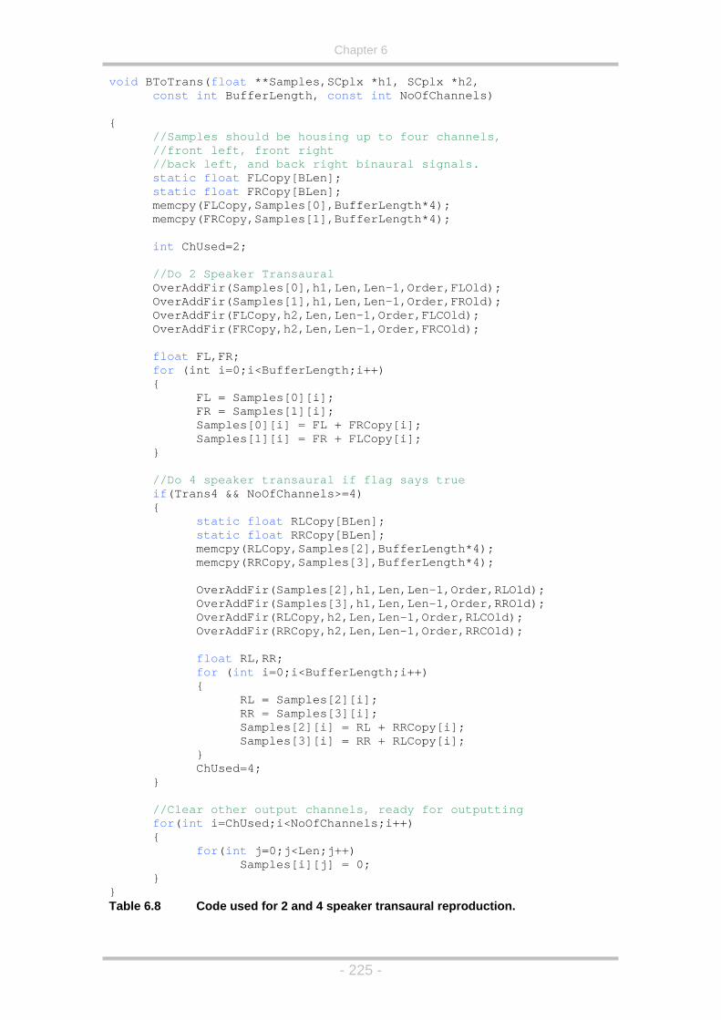
Chapter 6
void BToTrans(float **Samples,SCplx *h1, SCplxconst int BufferLength, const int NoOfCh
*h2, annels)
n,Len-1,Order,FLOld);
OverAddFir(FLCopy,h2,Len,Len-1,Order,FLCOld); OverAddFir(FRCopy,h2,Len,Len-1,Order,FRCOld); i++)
{ FL = Samples[0][i];
py[i];
{
static float RLCopy[BLen];
3][i]; = RL + RRCopy[i];
Samples[3][i] = RR + RLCopy[i]; }
{ //Samples should be housing up to four channels,
//front left, front right //back left, and back right binaural signals. static float FLCopy[BLen]; static float FRCopy[BLen]; memcpy(FLCopy,Samples[0],BufferLength*4); memcpy(FRCopy,Samples[1],BufferLength*4); int ChUsed=2; //Do 2 Speaker Transaural OverAddFir(Samples[0],h1,Le OverAddFir(Samples[1],h1,Len,Len-1,Order,FROld);
float FL,FR; for (int i=0;i<BufferLength;
FR = Samples[1][i]; Samples[0][i] = FL + FRCopy[i]; Samples[1][i] = FR + FLCo }
//Do 4 speaker transaural if flag says true if(Trans4 && NoOfChannels>=4)
static float RRCopy[BLen]; memcpy(RLCopy,Samples[2],BufferLength*4); memcpy(RRCopy,Samples[3],BufferLength*4); OverAddFir(Samples[2],h1,Len,Len-1,Order,RLOld); OverAddFir(Samples[3],h1,Len,Len-1,Order,RROld); OverAddFir(RLCopy,h2,Len,Len-1,Order,RLCOld); OverAddFir(RRCopy,h2,Len,Len-1,Order,RRCOld); float RL,RR; for (int i=0;i<BufferLength;i++) { RL = Samples[2][i]; RR = Samples[ Samples[2][i] ChUsed=4; } //Clear other output channels, ready for outputting for(int i=ChUsed;i<NoOfChannels;i++) { for(int j=0;j<Len;j++) Samples[i][j] = 0; } } Table 6.8 Code used for 2 and 4 speaker transaural reproduction.
- 225 -

Chapter 6
6.3 Implementation - Platform Specifics
All of the algorithmic work discussed so far in this project has been platform
independent, that is, all of the functions could be implemented on any pla
that supports floating point operations and standard C. However, there has
come a point where a specific platform must be chosen, and then more
specialised functions are usually needed
tform
to
depending on the
har icrosoft Windows™
ope t erfacing
wit
a system)
•
The system used in this project was the standard waveform audio system.
here were a number of reasons for this:
Although information about the Waveform Audio API is reasonably
widespread (for example, see Kientzle (1997) and Petzold (1998) Chapter 22)
none give a comprehensive guide to setting up a software engine for signal
processing (that is, capturing some audio live or from wave files, processing it,
and outputting the processed audio). For this reason, This section of the
report will give an in depth summary of how the software used in this project
was structured and implemented so it can be used as a starting reference for
ar
separate entity and programmed for accordingly. For example, just because
dware/operating system used. In this project the M
ra ing system was used, which possesses a number of APIs for int
h the sound system via Windows:
• Waveform Audio (windows multi-medi
• Direct Sound (part of the Direct X API)
ASIO (Steinberg’s sound API).
T
• Waveform audio had easy support for multi-channel sound.
• All windows compatible sound cards had good support for this API.
further rese ch to be carried out.
So, what is the Waveform Audio API? The Waveform Audio API is a layer of
functions that sits between the programmer and the sound card. This means
that the function calls necessary to set up and successfully run an audio
application will be the same no matter what make or model of sound card the
computer possesses. In this system the input and the output ports of the
soundcard work seemingly independently, and so each must be taken as a
- 226 -

Chapter 6
the output device has been set up as a 44.1 kHz, 16-bit sample stream, this
does not mean that the input device will automatically take these setting
when it is started. Any device act
s
ivated (be it input or output) using the
number of parameters set and structures
le, 8, 16).
.
Using all of the above data, the Waveform audio API is almost ready to set up
e input/output devices, however, let us first look at the block diagram of the
buffer and is ready for the next one.
e work in much the same way as software
in order to
waveform audio API must have a
available for use. Firstly, let us examine the parameters that must be set
before an output device can be started:
• Data type (for example, fixed or floating point).
• Number of Channels (for example, 1 – mono, 2 – stereo, 4, 8).
• Sample rate in Hz. (for example, 44100 or 48000).
• Bits per sample (for examp
• Block align – the alignment of the samples in memory (i.e. the size of
the data for one sample for all of the channels, in bytes)
• Average bytes per second.
• Buffer size in bytes.
th
waveform audio system as shown in Figure 6.10.
Figure 6.10 Waveform audio block diagram – Wave out.
As can be seen from this diagram, the soundcard actually informs the
program when it has finished with the last
This is because Windows is a message based operating system. That is, the
application either passes messages, or waits to receive messages from the
Windows operating system. Thes
interrupts on a D.S.P. device, and mean that the application does not have to
run in a loop, but process and send the appropriate messages
WaveHDR
WaveHDR
WaveHDR
WaveHDR
Send to Soundcard
Message: Ready for Samples
Processed Samples
- 227 -
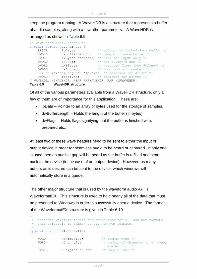
Chapter 6
keep the program running. A WaveHDR is a structure that represents a buffer
/* wave data block header */
buffer */ /* length of data buffer */
/* used for input only */
*/
erved for driver */
able 6.9 WaveHDR structure.
flags signifying that the buffer is finished with,
At least two of these wave e input or
tput device in order for s aptured. If only one
filled and sent
ver, as many
tom .
aveform audio API is
old nearly all of the data that must
lly open a device. The format
rmats. non-PCM formats.
/* format type */
ste
of audio samples, along with a few other parameters. A WaveHDR is
arranged as shown in Table 6.9.
typedef struct wavehdr_tag { LPSTR lpData; /* pointer to locked data
DWORD dwBufferLength; DWORD dwBytesRecorded; DWORD dwUser; /* for client's use */ DWORD dwFlags; /* assorted flags (see defines) DWORD dwLoops; /* loop control counter */ struct wavehdr_tag FAR *lpNext; /* reserved for driver */ DWORD reserved; /* res} WAVEHDR, *PWAVEHDR, NEAR *NPWAVEHDR, FAR *LPWAVEHDR; T Of all of the various parameters available from a WaveHDR structure, only a
few of them are of importance for this application. These are:
• lpData – Pointer to an array of bytes used for the storage of samples.
• dwBufferLength – Holds the length of the buffer (in bytes).
• dwFlags – Holds
prepared etc..
headers need to be sent to either th
ou eamless audio to be heard or c
is used then an audible gap will be heard as the buffer is re
back to the device (in the case of an output device). Howe
buffers as is desired can be sent to the device, which windows will
au atically store in a queue
The other major structure that is used by the w
WaveformatEX. This structure is used to h
be presented to Windows in order to successfu
of the WaveformatEX structure is given in Table 6.10. /* * extended waveform format structure used for all non-PCM fo * this structure is common to all / *
typedef struct tWAVEFORMATEX {
wFormatTag; WORD WORD nChannels; /* number of channels (i.e. mono,
reo...) */ DWORD nSamplesPerSec; /* sample rate */
- 228 -

Chapter 6
DWORD nAvgBytesPerSec; /* for buffer estimation */ ck size of data */
of extra information (after
NPWAVEFORMATEX, FAR WAVEFORMATEX;
w potentially available for any device that is to be
evice.
on to
information and memory allocation needed. Example
evice is shown in Table 6.11. r[2];
hWa
if(Device==0)
{ WOutHdr[i].dwBufferLength = usBLength * wf.wBitsPerSample
* wf.nChannels/8; WOutHdr[i].lpData = new char[WOutHdr[i].dwBufferLength];
WORD nBlockAlign; /* blo WORD wBitsPerSample; /* number of bits per sample of
mono data */ WORD cbSize; /* the count in bytes of the size
cbSize) */} WAVEFORMATEX, *PWAVEFORMATEX, NEAR **LPTable 6.10 WaveformatEX structure. As can be seen by the comments in Table 6.9 and Table 6.10, all of the
necessary information is no
opened, be it an input, or an output d
Various functions are used in the initialisation and running of a Wave device
and the structures given in Table 6.9 and Table 6.10 are relied up
provide the necessary
code used to initialise a wave out dWAVEHDR WOutHdWAVEFORMATEX wf; AVEOUT veOut; HW
void InitialiseWaveOut( unsigned int Device,
unsigned short usNoOfChannels, unsigned short usSRate, unsigned short usBLength)
{ //Pass WAVEFORMATEX structure necessary data wf.wFormatTag = WAVE_FORMAT_PCM; wf.nChannels = usNoOfChannels; wf.nSamplesPerSec = usSRate; wf.wBitsPerSample = 16; wf.nBlockAlign = wf.nChannels * wf.wBitsPerSample / 8; wf.nAvgBytesPerSec= wf.nSamplesPerSec * wf.nBlockAlign; wf.cbSize = 0; //let windows choose device Device=WAVE_MAPPER; else //else, use specified device Device--; //Open wave device, specifying callback function //used to catch windows messages from device waveOutOpen(&hWaveOut,Device,&wf,(DWORD)WOCallback, (DWORD)this,CALLBACK_FUNCTION); waveOutPause(hWaveOut); //Allocate memory for 2 buffers, and pass them to wave device for(int i=0;i<2;i++)
- 229 -

Chapter 6
WOutHdr[i].dwFlags = 0; WOutHdr[i].dwLoops = 0; waveOutPrepareHeader(hWaveOut,&WOutHdr[i],sizeof(WOut waveOutWrite(hWaveOut,&WOutHdr[i],sizeof(WOutHd } //Start wave out device waveOutRestart(hWaveOut); } //----------------------------------------------------------------void CALLBACK WaveOutCallback(HWAVEOUT hwo, UINT uMsg, DWORD dwInstance, DWORD dwParam1, DWORD dwParam2) { switch(uMsg) { case WOM_DONE: { //If WOM_DONE, call function used to fill buffe //WAVEHDR buffer passed in to callback function //as dwParam1 WaveOutFunc((WAVEHDR *)dwParam1); break; } default: break; } } Table 6.11 Initialisation code used to set up and start an output wave device. As shown in Table 6.11, a call-back function must be specified in ord
Hdr[i])); r[i]));
---
r
er to
process the Windows’ messages that are passed by the waveform audio
system. For the output device the most important message is WOM_DONE.
This message is passed to the call-back function every time the wave out
device has finished with the WAVEHDR buffer, where a function can then be
called that fills the buffer with processed samples using the processing
techniques shown in Chapter 6.2 (in this case, the WaveOutFunc function is
called, passing with it a WaveHdr structure).
The Wave In device is configured in much the same way by the Windows
operating system, although it is interesting to note that the input and output
devices are both taken to be two separate devices. To this end, no automatic
connection between the two devices exists and it is the programmer that must
ourse, assuming that both input and output devices have been initialised at
store the input samples and then pass them to the output device (this is, of
c
the same frequency, bit rate and channel numbers).
- 230 -

Chapter 6
In Windows, many audio devices can be opened simultaneously, which is
necessary as most multi-channel sound cards default to being configured as a
numbe
r of stereo devices. However, for true multi-channel sound
reproduction it is necessary to have a card that can be configured as one
multi-channel device. This is due to the fact that Windows cannot open and
start multiple devices at exactly the same time and, although some sound
card manufacturers quote that the drivers will synchronise multiple devices,
this has not been found to be the case when using their standard wave
drivers. This can potentially cause problems when using such a card to feed
an array of speakers used for multi-channel surround sound, as the time
alignment of the output channels is assumed to be perfect. Although this
artefact is not readily noticeable, it is obviously more desirable to start with a
system that is as theoretically perfect as possible and so a single multi-
channel device should be used, if possible. Having one multi-channel device
This effect wa he Matlab add-on, Simulink. The block
also simplifies the processing as multiple call-back functions are not used.
s discovered using t
arrangement used to document this feature is shown in Figure 6.11.
Figure 6.11 Simulink model used to measure inter-device delays
This system was used to test the latency of various devices a number of times
four
and not only was the inter-device latency apparent, but it also changed
between test runs. An example plot is shown in Figure 6.12, showing just
- 231 -

Chapter 6
devices, to make the graph more readable. This variable device latency
means that it is almost impossible to correct, and so a single device should be
used.
0 2000 4000 6000 8000 10000 12000-0.3
-0.25
-0.2
-0.15
-0.1
-0.05
0
0.05
0.1
0.15
0.2
time in samples at 44.1KHz sampling frequency
Delay between opening of devices
mag
nitu
dedevice 1device 2device 3device 4
Figure 6.12 Graphical plot of the output from 4 audio devices using the Waveform
audio API.
In order to successfully close an audio device, a number of API calls must be
made. This is shown (for the output device) in Table 6.12. void CloseDevice(UINT Device) { //Reset Wave Device
waveOutReset(hWaveOut); //Unlock and delete dynamic memory allocated for WAVEHDRs
for(UINT i=0;i<NoOfBuffers;i++) {
waveOutUnprepareHeader(hWaveOut,&WaveHeadersOut[i], sizeof(WaveHeadersOut[i]));
if(WaveHeadersOut[i].lpData) delete [] WaveHeadersOut[i].lpData;
}
the
//Close Wave Device
waveOutClose(hWaveOut); } Table 6.12 Closing a Wave Device Both the opening and closing of an input wave device is identical to that of an
output wave device, with the only difference being the message passed to
call-back function.
As all of this coding is Windows dependent (that is, it will never be needed for
any other system), the wave device functions were encapsulated within a
- 232 -

Chapter 6
class. This meant that a basic ‘pass-through’ application could be coded, tha
did no processing. A ne
t
w class could then be created, inheriting from this first
edeclared so that minimal extra
to be
nal processing
g and outgoing samples has been written. This
r processed) just after the input and
just be
lass is shown in Figure 6.13.
dy
audio
ata to a data queue. Then, when the WOM_DONE message has been
class, but with the processing functions being r
coding is needed for every new sound processing application that is
written.
In order for this first class to be as flexible as possible, a sig
function for both incomin
means that the signal can be monitored (o
fore the output of the audio to the soundcard.
A block diagram of the structure of this c
Figure 6.13 Block Diagram of Generic ‘pass-through’ Audio Template Class It can be seen from Figure 6.13 that, apart from the initialisation and opening
of the audio devices, the whole of the audio subsystem is driven by
messages. The WIM_DATA message signalling that an audio buffer is rea
for use (i.e. full) causes the WaveInFunc to call a function that adds this
d
received signalling that an output buffer is ready to be filled again, the
ProcessOut function is called, which is where the audio processing will be
carried out on the data at the end of the audio queue, and then passed to the
empty output device. An example of the overridden ProcessOut function is
Initialise
Init & Allomemory for
c
WaveHDRs Create Sample Queue
Open Device
Open In/Out Devices Prepare & Send Buffers to devices Start Devices
WaveInFunc
Call AddToQueue Add Used Buffer to device
WaveOutFunc
Call Process Out Add Used Buffer to device
AddToQueue
Add new samples to audio queue
ProcessIn
Function to beOverRidden
ProcessOut
Function to be OverRidden
Calls made from Application
WIM_DATA Message
WOM_DONE Message
Invoked by Windows Messages
- 233 -
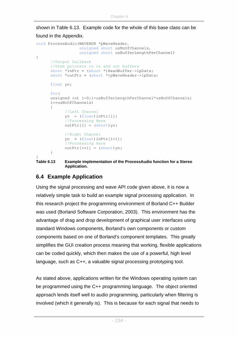
Chapter 6
shown in Table 6.13. Example code for the whole of this base class can be
found in the Appendix. void ProcessAudio(WAVEHDR *pWaveHeader,
unsigned short usNoOfChannels, unsigned short usBufferLengthPerChannel) { //Output Callback //Grab pointers to in and out buffers
short *inPtr = (short *)ReadBuffer->lpData; short *outPtr = (short *)pWaveHeader->lpData; float yn;
for( unsigned int i=0;i<usBufferLengthPerChannel*usNoOfChannels; i+=usNoOfChannels)
{ //Left Channel yn = (float)inPtr[i]; //Processing Here outPtr[i] = (short)yn; //Right Channel yn = (float)inPtr[i+1]; //Processing Here outPtr[i+1] = (short)yn; } } Table 6.13 Example implementation of the ProcessAudio function for a Stereo
Application.
6.4 Example Application
Using the signal processing and wave API code given above, it is now a
task to build an example signal processing application. In
onment of Borland C++ Builder
orporation, 2003). This environment has the
s using
orland’s own components or custom
emplates. This greatly
tions
relatively simple
this research project the programming envir
was used (Borland Software C
advantage of drag and drop development of graphical user interface
standard Windows components, B
components based on one of Borland’s component t
simplifies the GUI creation process meaning that working, flexible applica
can be coded quickly, which then makes the use of a powerful, high level
language, such as C++, a valuable signal processing prototyping tool.
As stated above, applications written for the Windows operating system can
be programmed using the C++ programming language. The object oriented
approach lends itself well to audio programming, particularly when filtering is
involved (which it generally is). This is because for each signal that needs to
- 234 -

Chapter 6
be filtered, separate memory locations are needed for that particular signa
feedback, feedforward, or delay line features. When coding filters in C it is the
developer th
l’s
at must group all of this memory together, which can be
umbersome at times with different types of filters needing different memory
red.
at
f
s object,
rocessaudio’ function.
simple template for such a class is shown in Table 6.14.
Buffer;
fLen; ss(float *signal, int iLen, float aval);
; gnal, float dBLP, float dBHP,
lisation unit.
of t in the
object must be initialised with an integer length (see the constructors and
c
requirements. For example, the fast convolution algorithm described in
section 6.2.2 needs an additional amount of memory for each channel filte
The size of this memory must be the same size as the FFT window size, th
is, it must be larger than the size of the incoming signal. Once other types o
filter are also introduced the subsequent memory requirement would soon
become complicated and difficult to follow. This, on its own, is not a large
problem, but means that all the memory requirements for a filter function must
be clearly documented using comments, and strictly adhered to by the
developer. However, in C++ a filter ‘object’ can be created. Inside thi
all the extra memory requirements can be hidden from the programmer with
as many filter objects created as needed. This means that each filter object
can be imagined as one filter device in a studio, operating on one audio
stream. Initially, all the same memory requirements must be taken care of,
but once implemented inside a C++ class this can then be used as a template
where the developer only has access to, perhaps, a ‘p
Aclass AllPass { private: float fs,fc,alpha,* float ff,fb,in,out; const int Bu
void DoAllPa public: AllPass(int iLen); ~AllPass();
float fsam) void SetCutOff(float fcut,id ProcessAudio(float *si vo
bool dBdummy); (float *signal, float LinLP, float LinHP); void ProcessAudio
}; ss based shelving equaTable 6.14 C++ Class definition file for an allpa
An object ype AllPass can now be initialised in the normal way
application. However, due to the fact that the private variable BufLen,
representing the length of an audio buffer, has been declared constant, this
- 235 -

Chapter 6
destructors, AllPass(int iLen) & ~AllPass()). This means that, unless the
application has a fixed buffer length, the object must be declared dynamically
er it can be seen that the developer
; a constructor and a destructor that are
ct is created or destroyed, a
o functions. The latter have been
proved flexibility, with one function making
aking use of dB gain values. As the
difference in their passed values, a
d in one of the functions to indicate
e variables
wi , meaning that the calling object
s no access to these variables, protecting them from potential wrong doing.
in the
ures that
FLength);
oat *signal);
e fast convolution algorithm
lass definition
er, if the constructor of this class is shown, it can be
at run time.
Looking at this object definition file furth
only has access to five functions
called automatically when a new AllPass obje
SetCutOff function, and two ProcessAudi
created in order to give this class im
use of linear gain values, and the other m
same function names need to have some
dummy, unused variable has been include
that dB gains are used. Also, it can be noted that all of th
associated th this class are declared private
ha
All of these variables are updated, as needed, by the underlying code
class, either at initialisation, or by a public member function. This ens
the filter is secure and as intuitive to use as possible, with the developer only
having access to the functions needed, and no more.
This method was also used for the fast convolution filter, greatly simplifying
the knowledge needed by the developer to use this function. The definition
file is shown in Table 6.15. class FastFilter { private: int order,fftsize,siglen,implen; float *OldArray,*Signal,*tconv,*h; SCplx *fh,*fSig,*fconv; public: FastFilter(int FFTOrder,AnsiString *FName,int ~FastFilter(); void ReLoadFilter(AnsiString *FName,int FLength); void OverAddFir(fl};
++ class definition file for thTable 6.15 C Again, a system very similar to that shown in the AllPass filter c
file can be seen. Howev
- 236 -

Chapter 6
seen how much work is taken away from the developer when using this class,
e 6.16. me,int FLength)
float[fftsize];
Length);
s is immediately evident, the memory requirements of this class are
into
s
r
6.17 and Table 6.18 respectively. fun i%save array to .dat file for reading in a c program % for example count = savearray(array,'c:\coefs.dat'); fid = fopen(fname, cou fclose(fid); Table 6.17 tion used to write FIR coefficients to a file. #include <fstream.h> void FastFilter::ReLoadFilter(AnsiString *FName,int FLength) {
as shown in TablFastFilter::FastFilter(int FFTOrder,AnsiString *FNa{ order = FFTOrder; fftsize = pow(2,order); siglen = (fftsize/2) + 1; implen = fftsize/2; OldArray = new float[fftsize]; Signal = new float[fftsize];
= new float[fftsize]; tconv = new h
; fh = new SCplx[fftsize]
fSig = new SCplx[fftsize]; fconv = new SCplx[fftsize];
LoadFilter(FName,F Re nspsRealFftNip(NULL,NULL,order,NSP_Init); nspsRealFftNip(h,fh,order,NSP_Forw); } Table 6.16 Constructor for the FastFilter class A
complicated, with a number of memory spaces of two variable types
(representing data in both the time and frequency domain) needing to be
dynamically created and destroyed when necessary. Also, the size of the
coefficients used in FIR filters can be large, meaning that entering them
the code is unfeasible. So, this class actually takes in a filename that contain
the list of numbers used in the filter, in single precision format. This means
that the filters can be quickly designed and saved to a file format in Matlab,
and then tested quickly using a C++ Windows application without the need fo
any changes in the code of the application, meaning that recompilation is not
necessary. The Matlab code used to create these files and the C++ code
used to read them are shown in Table ct on count = savearray(array, fname);
'w'); nt = fwrite(fid,array,'float');
Matlab func
- 237 -

Chapter 6
F ze); ); memset(tconv,0,sizeof(float)*fftsize); memset(h,0,sizeof(float)*fftsize); memset(fh,0,sizeof(SCplx)*fftsize); memset(fSig,0,sizeof(SCplx)*fftsize); memset(fconv,0,sizeof(SCplx)*fftsize); f = fopen(FName->c_str(),"rb"); i { c = fread(h,sizeof(float),FLength,f);
pplication can be designed. This example application was designed to test a
e
archived), or one mono
ave file for panning into a B-format signal. If a mono source is used, then
this can be panned using a rotary dial, and if a B-format signal is used, then
the sound field can be rotated using a rotary dial. The user is able to choose
from four different decoding methods:
• Optimised eight speaker regular Ambisonics (using the allpass filters
described above).
• Ambisonics to binaural transform (based on an eight speaker array).
• Ambisonics to two speaker transaural with speaker placements at:
o +/- 30
o +/- 50
o +/- 100
o +/- 200
ILE *f; int c;
memset(OldArray,0,sizeof(float)*fftsi memset(Signal,0,sizeof(float)*fftsize
f(f)
if(c!=FLength) MessageBox(NULL,"Filter Length Error",
"Filter Length Error", NULL); fclose(f); } else MessageBox(NULL,"Cannot open file",
"Cannot open file", NULL); } Table 6.18 C++ code used to read in the FIR coefficients from a file.
Now the main signal processing classes have been constructed, the
a
number of the optimisation techniques discussed in Chapter 5. However, th
irregular Ambisonic array testing was carried out in Simulink, and is not
implemented in this application in order to keep things a little simpler. It will
be capable of taking in a first order B-format signal (comprised of four wave
files, as this is how most of our B-format material is
w
- 238 -

Chapter 6
o +/- 300
• Ambisonics to four speaker transaural with front speaker placements
as above, and rear speaker placements at:
o +/- 50
o +/- 100
o +/- 200
o +/- 300
o +/- 700
In addition to these modes of reproduction, a source from the line input can
also be used so that the transaural filters (two speaker algorithm) can be
er to utilise
ll of the transforms discussed above, a total of fifty six filters must be made
ne
sam her reason
why writing these to separate data files saves time and programming effort.
rota e discussed
her h
tested with CD material (both binaural and normal stereo). In ord
a
available to the application as there must be two versions of each filter. O
pled at 44.1 kHz and another sampled at 48 kHz. This is anot
To facilitate the above formats, a GUI was constructed as shown in Figure
6.14. All of the controls used are standard Windows controls, apart from the
two rotary controls used for altering the mono source panning and b-format
tion. The code for the creation of the rotary controls will not b
e, owever, but can be found in the Appendix.
- 239 -

Chapter 6
Figure 6.14 Screen shot of simple audio processing application GUI.
In the audio subsystem class, there are two main tasks to be carried out:
• Initialisation/deinitialisaton of filter structures and graphical
oscilloscope.
• Process audio function.
In order for to avoid storing fifty six FIR filters in memory at once (and, for that
matter, having to manage fifty six FIR filter structures in the program code),
only the filters currently available for use will be stored in memory. These are:
• 3 Allpass filters for the eight speaker Ambisonic decoder.
• 3 FIR filters for Ambi to two ear binaural processing
• 6 FIR filters for Ambi to four ear binaural processing
• 4 FIR filters for binaural to two speaker transaural processing
• 4 FIR filters for binaural to four speaker transaural processing (8 used
in this algorithm in total).
is only the crosstalk cancellation filters that need to be updated in real time,
filter
function for this application is shown in Figure
5.
It
and so, in order to facilitate this, the GUI sets a flag to true whenever a
needs changing (that is, the transfilter and rear filter radio boxes are
changed). The audio subsystem checks this flag at the start of every audio
buffer and, if set, reloads the appropriate filter from disk.
A block diagram of the audio
6.1
- 240 -
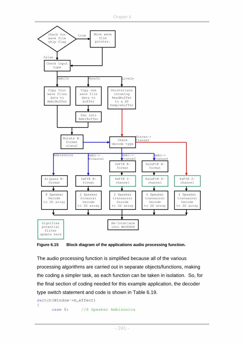
Chapter 6
Move wave Check for true file
pointer. wave file skip flag
false
Check input type
AmbiIn MonoIn LiveIn
of the applications audio processing function. Figure 6.15 Block diagram
The audio cessing function is simplified because all of the va pro rious
g
a simpler task, as each function can be taken in isolation. So, for
the final section of coding needed for this example application, the decoder
nd code is shown in Table 6.19.
processing algorithms are carried out in separate objects/functions, makin
the coding
type switch statement aswitch(Window->m_effect) { case 0: //8 Speaker Ambisonics
Ambi-> Ambi-> Transx4 Transx2
Copy four Copy one wave files data to
AmbiBuffer
wave file data to buffer
Deinterlace incoming
ReadBuffer to a 2D
Samplebuffer
Pan into iBuffer Amb
Rotate B-format signal
Check decode type
Allpass B-format
8 Speaker Decode
to 2D array
3xFIR B-format
2 Speaker binaural
ecode Dto 2D array
4xFIR 2-channel
2 Speaker saural tran
Decode to 2D array
4x2xFIR 4-channel
4 Speaktransau
er ral
Decode to 2D array
2 Speaker transaural
Decode to 2D array
3xFIR B-format
3x2xFIR B-format
4xFIR 2-channel
Ambisonics Ambi-> Binaural
Re-Interlace into WAVEHDR
Stereo->Transx2
Signifies potential filter
update here
- 241 -
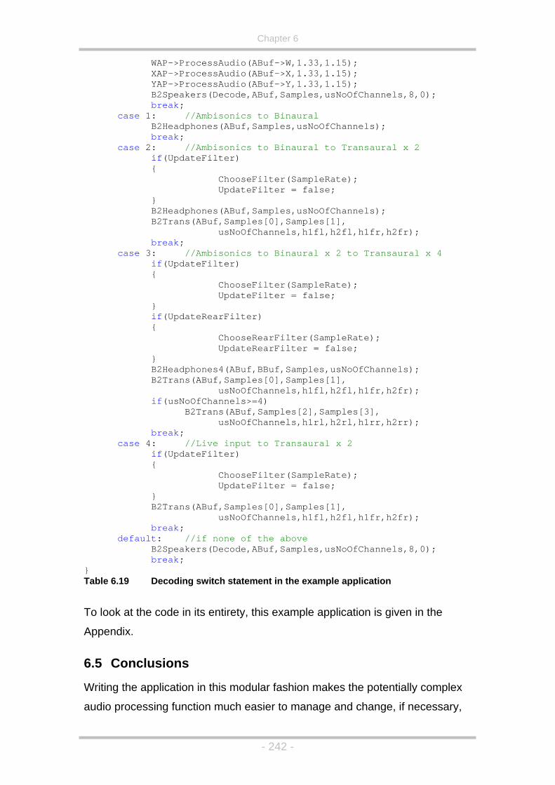
Chapter 6
WAP->ProcessAudio(ABuf->W,1.33,1.15); XAP->ProcessAudio(ABuf->X,1.33,1.15); YAP->ProcessAudio(ABuf->Y,1.33,1.15);
B2Speakers(Decode,ABuf,Samples,usNoOfChannels,8,0); break;
B2Headphones(ABuf,Samples,usNoOfChannels); B2Trans(ABuf,Samples[0],Samples[1],
Buf,BBuf,Samples,usNoOfChannels); mples[0],Samples[1],
usNoOfChannels,h1fl,h2fl,h1fr,h2fr); if(usNoOfChannels>=4)
B2Trans(ABuf,Samples[2],Samples[3], usNoOfChannels,h1rl,h2rl,h1rr,h2rr); break; case 4: //Live input to Transaural x 2 if(UpdateFilter) { ChooseFilter(SampleRate); UpdateFilter = false; } B2Trans(ABuf,Samples[0],Samples[1], usNoOfChannels,h1fl,h2fl,h1fr,h2fr); break; default: //if none of the above B2Speakers(Decode,ABuf,Samples,usNoOfChannels,8,0); break; } Table 6.19 Decoding switch statement in the example application
To look at the code in its entirety, this example application is given in the
Appendix.
6.5 Conclusions
Writing the application in this modular fashion makes the potentially complex
audio processing function much easier to manage and change, if necessary,
case 1: //Ambisonics to Binaural B2Headphones(ABuf,Samples,usNoOfChannels); break; case 2: //Ambisonics to Binaural to Transaural x 2 if(UpdateFilter) { ChooseFilter(SampleRate); UpdateFilter = false; } usNoOfChannels,h1fl,h2fl,h1fr,h2fr); break; case 3: //Ambisonics to Binaural x 2 to Transaural x 4 if(UpdateFilter) { ChooseFilter(SampleRate); UpdateFilter = false; } if(UpdateRearFilter) { ChooseRearFilter(SampleRate); UpdateRearFilter = false; } B2Headphones4(A B2Trans(ABuf,Sa
- 242 -

Chapter 6
and has resulted in a large library of functions and classes that can be used to
application very quickly.
st convolution algorithm, and the utilisation of the Intel
the
stead (Intel, 2003b)),
the
proces
Most o as carried out in Matlab and
Sim
Chapte
custom r
Binaur
based
invalua
filte
create a working multi-channel audio
Due to the use of the fa
Signal Processing Library (although Intel have now discontinued this, and
Intel Integrated Performance Primitives must be used in
implemented surround sound system will run on Intel Pentium II
sors and faster, even when decoding to eight or more speakers.
f the Ambisonic algorithmic testing w
ulink, but regarding sound quality, the software libraries described in this
r work well and without audio glitches. It must also be noted that using
C software was the only way to test and evaluate the Transaural o
al decoders in real-time due to the lack of a real-time (that is, frame
) overlap add convolution function in Simulink, so this software was
ble in the rapid evaluation and testing of the crosstalk cancellation
rs described in Chapter 5.
- 243 -

Chapter 7
Chap
7.1 I
This th
surrou
1.
, the
2. ntal 1st order d order
by
ally, and later by Noisternig et al. (2003),
none of this work takes into account the correct presentation of the
latera addressed in point 1, above.
3. Only d decoding of
and no
psychoacoustically correct decoding software for irregular arrays exists.
ch as follows:
1992)
Ambisonic
decoders for irregular speaker arrangements using the velocity and
h
d in
esign
of multi-channel decoders. This form of decoder is not strictly
Ambisonic, as it does not conform to the Ambisonic definition as
described by Gerzon & Barton (1998) and described in section 3.3.1,
but will allow for the further optimisation of the B-Format decoding
ter 7 - Conclusions
ntroduction
esis has identified the following problems with the current state of
nd sound systems (as described in Section 3.4):
Although Gerzon and Barton (1992) suggested a number of
optimisation equations for use with irregular speaker arrangements
equations are difficult to solve, and so no further research seems to
have been carried out in this area.
At least four speakers must be used to decode a horizo
signal, and six speakers must be used to decode a horizontal 2n
system and although the conversion to binaural has been done
McKeag & McGrath (1996) initi
lisation parameters which has been
a handful of software utilities for the encoding an
Ambisonic material are available (McGriffy, 2002),
These problems have been addressed in this resear
1. A method of solving the equations given by Gerzon and Barton (
has been demonstrated that simplifies the design of
energy vector criterion as described by Gerzon & Barton (1992) whic
also corrects the problem of low and high frequency decoder
discrepancies as shown in section 5.3.
2. Also, a new method of HRTF analysis has been developed in order to
differentiate between decoders designed using the method describe
point 1, above. This data has then been utilised directly in the d
- 244 -

Chapter 7
process than is possible using the original velocity/energy vector theory
(i.e. more frequency bands can be used).
3. The use of B-format and higher order Ambisonic encoded signals as a
carrier format for Binaural and Transaural reproduction systems has
been demonstrated. The optimisation of both Binaural and Transaural
techniques through the use of inverse filtering has been formulated,
with the transaural reproduction technique benefiting particularly from
this technique. Also, a new Ambisonic to four speaker Transaural
decode has been formulated and discussed, although sound quality
used in
onic carrier signal over:
The de
7.2 Ambisonics Algorithm development
This project has concentrated on t
surround sound format based on the Ambisonic system.
The traditional method of analysing and optimising Ambisonic decoders is
through the use of the energy and velocity vector theories. The algorithmic
development in this report, in the most part, has been centred on the use of
HRTF data in order to analyse and optimise the performance of the Ambisonic
decoders directly. This form of analysis was shown, in Chapter 5, to give
results that backed up the original energy and velocity vector theory.
issues have hindered this work, possibly due to the HRTF set
this research, and so work in this area is still ongoing.
4. Software utilities have been implemented for both the design of
decoders for irregular speaker arrays, and the replaying of the
Ambis
a. Headphones
b. Two or four speaker Transaural
c. Multi-speaker, optimised, Ambisonic arrays.
tails of these achievements are discussed below.
he decoding of a hierarchical based
- 245 -

Chapter 7
600
1400
800 800
600
1400
800 800
Figure 7.1 Recommended loudspeaker layout, as specified by the ITU.
That is, if an Ambisonic decoder was optimised using the energy and velocity
vectors, then this result also gave a very good match when analysed using the
HRTF method. A number of interesting observations were made from this
experiment:
• Although a standard ITU five speaker arrangement was used (as
shown in Figure 7.1) in the analysis and optimisation stages, the
velocity vector analysis gave a perfect low frequency match for the
decoder, as shown in Figure 7.2. This was surprising as there is such
a large speaker ‘hole’ at the rear of the rig.
• However, the HRTF analysis showed some error in the rear of the
sound fields reproduction, which seems to show a more realistic resu
as demonstrated in Figure 7.3.
lt,
Figure 7.2 Low frequency (in red) and high frequency (in green) analysis of an
optimised Ambisonic decode for the ITU five speaker layout.
- 246 -

Chapter 7
2HF Amp Difference
0 50 100 150 200 250 300 350 400-40
-20
0
20
40LF Time Difference
Tim
e D
iffer
ence
(sam
ples
)
Figure 7.3 A graph showing a real source’s (in red) and a low frequency decoded source’s (in blue) inter aural time differences.
Also, a number of benefits were found due to the inherent increased flexibility
of the HRTF analysis technique when compared to the analysis using the
energy and velocity vectors. Using the HRTF technique, the effect of head
movements could be analysed in a quantitative manner. This can prove
invaluable when trying to differentiate between a number of potentially optimal
sets of decoder coefficients, and significant differences can be observed. For
example, see Figure 7.4 which shows a comparison between two sets of
optimised decoder coefficients (using energy and velocity vector theory) and
their analytical performance under head rotation. One prominent feature of
Figure 7.4 can be seen if the low frequency time difference plots for a source
at 00 are observed. The second coefficients response to head rotation shows
that the time difference stays at roughly zero samples no matter what direction
the listener is facing, indicating that the source is tracking with the listener.
However, the first coefficients low frequency graphs shows that the time
difference of a source at 00 changes in the same way as a real source would,
that is, the source does not track with the listener and more correct cues are
presented.
- 247 -

Chapter 7
Coefficient Set 1
Coefficient Set 2
Figure 7.4
HRTF Simulation of head movement using two sets of decoder coefficients.
- 248 -

Chapter 7
Su nce
can giv
previo
Although the Vienna decoding optimisation technique (using the velocity and
t
this paper’s publication.
tool,
nd
ithout head-turning considerations.
or
, source.
ening to
recording.
Although a very small test base was used, decoders optimised using both
energy/velocity vectors and HRTF data directly, via the Tabu search
algorithm, were shown to outperform the reference decoder in both tests. The
best performing decoder in test 1 was an expected result, after observing the
performance of the decoder using HRTF data. However, the decoder that
was chosen unanimously as the preferred choice when auditioning pre-
recorded material was not as easy to predict. Reasons for this may be:
best, w
depen
ch observed variations between different decoders’ analytical performa
e more indications as to how well the decoder will perform than
us techniques allow.
energy vectors) was proposed in 1992, very little (if any) Vienna decoders
have been calculated and used, mainly due to both the mathematical
complexity in deriving decoder coefficients using this method and the fact tha
Gerzon’s paper gave results for a speaker layout very different from the ITU
standard, which was proposed after
To this end, software based on a Tabu search algorithm was developed that,
once the five speaker positions were entered, would calculate optimised
decoders automatically. This heuristic mechanism has proved a valuable
and once the program was written to optimise decoders using the Vienna
equations, it could easily be adapted to use the HRTF method, both with a
w
A limited set of formal listening tests have been carried out on a number of
decoders optimised using the two techniques described above, as a precurs
to further research in this area. Two tests were carried out:
1. Perceived localisation of a panned, dry
2. Decoder preference when list an excerpt of a reverberant
1. The most accurate decoder may not be the one that actually sounds
hen replaying pre-recorded material, and will be material
dant.
- 249 -

Chapter 7
2. It was noticed that the two best (analytically speaking) performing
when auditioned in the sweet-spot, which was not apparent with the
ed
This re for
spatial
availab
order t
and
Overa
can reproduce phantom images both to the side and behind the listener.
Howev
decod
differe d in this test (especially for test 1).
It has
order d
decod
below. 3) and another optimised using the
Tabu search methodology described above. n (2003)
optimised decoders exhibited a slightly uncomfortable, in-head, sound
preferred decoder. This effect disappeared when the listener mov
slightly off-centre.
sult suggests that when designing decoders artistically, rather than
accuracy, other parameters may need to be taken into account or be
le to the user so intuitive control of the decoder can be carried out in
o alter the spatial attributes of the presentation (such as spaciousness
perceived depth, for example).
ll the tests were encouraging and showed that the Ambisonic technique
er, a much larger test base should be used to further test the new
ers, along with more source positions, due to the reasonably subtle
nces between the decoders use
also been shown how this software can be adapted to optimise higher
ecoders for irregular arrays, as described by Craven (2003) and two
ers for such a system (using 4th order circular harmonics) are shown
One suggested by Craven (200
Decoder optimised using Tabu Search Decoder proposed by Crave
Figure 7.5 Energy and Velocity vector analysis of two 4th order, frequency
independent decoders for an ITU five speaker array. The proposed Tabu search’s optimal performance with respect to low frequency vector length and high/low frequency matching of source position can be seen clearly.
- 250 -

Chapter 7
7.2.1 Further Work
This project has raised a number of questions and results that require future
work:
1. Altering the coefficients of decoders (i.e. their virtual microphone
patterns) can drastically alter how reverberant a recording is perceived
to be (as well as altering other spatial attributes). This is probably
related to the amount of anti-phase components being reproduced fro
speakers, but needs further work to the relationship between mor
complex spatial attributes and decoder coefficients can be formulated..
2. The uncomfortable, ‘in-head’ perception reported by the listening test
subjects when listening to pre-recorded material requires further wor
which could be coupled into a study of how optimising decoders affects
its off-centre performance.
3. Altering the optimisation criterion to take into account off-centre
positions could be i
m
e
k
nvestigated so determine whether the sweet area of
the system can be increased.
4. A study of the higher order decoders, such as the one proposed by
Craven (2003), or decoders optimised using the Tabu search method,
as described in section 5.3.4, in order to evaluate what effect higher
order components have, and whether an upper limit, with respect to
harmonic order, can be judged.
7.3 Binaural and Transaural Algorithm Development
7.3.1 B-format to Binaural Conversion
The main optimisation method employed using the decoding technologies
based on binaural techniques is that of inverse filtering. This is needed for the
HRTF set used in this report due to the noticeable colouration of the sound
perceived when these HRTFs are used. The inverse filtering technique works
well in improving the quality of these filters, while maintaining their
performance, as the differences between the ears remain the same and the
pinna filtering is likely to be incorrect when compared to that of a listener’s (in
fact, the likelihood of the pinna filtering being the same is extremely slim, if not
possible). However, the B-format HRTFs created (see Figure 7.6) do give im
- 251 -

Chapter 7
the impression of a more spatial headphone reproduction, when compa
listening in conventional stereo, even though these are the anechoic forms of
the filters. This is especially true when listening to sounds recorded in
reverberant fields as the ear/brain system will now receive more coherent
cues than when mixing the B-format to it’s stereo equivalent (which is based
on mid and side microphone signals and relies on the crosstalk between
ears which is destroyed using headphones – see section 3.2.2 on Blumlein
Stereo for more details). Two recordings have been obtained from the
company Serendipity (2000) where recordings of the musicians were made
Lincoln Cathedral using both
red to
the
in
a SoundField microphone and a binaural, in-ear
system, simultaneously. Although the binaural recording was not from the
n, a binaural sound artist,
uld be
same position (it was carried out by Dallas Simpso
who tends to move around often during recordings for artistic effect), a
qualitative comparison of the spatial qualities of the two recordings co
made over headphones.
Figure 7.6 B-format HRTF filters used for conversion from B-format to bina
decoder.
ural
- 252 -

Chapter 7
This confirmed that the B-format to binaural system seems to perform
favourably when compared to the plain binaural system, although good out
head effects are still difficult to achieve with both recordings. This is not due
to algorithmic erro
of
rs, but to the fact that the ear/brain system isn’t receiving
nough coherent cues, and it is interesting as the work by Lake (McKeag &
ith their large hall
imp s
impuls
7.3.2
On t
chann
employing the filter design techniques outlined and discussed in Chapter 5.
The inverse filtered crosstalk cancellation filters perform better when
auditioning standard binaural material when compared to binauralised B-
Format material, with colouration of the sound being noticeable when replying
B-Format in this way, although the colouration is not noticeable when
auditioning either the B-Format to binaural, or binaural to crosstalk cancelled
material in isolation.
As mentioned in Chapter 5, pinna errors seem to worsen the system’s
accuracy and, to this end, the Ambiophonics system employs a pinna-less
dummy head in the calculation of the inverse filters for the crosstalk
cancellation, and in the recording of the event itself (Glasgal, 2001).
7.3.3 Binaural to Four Speaker Transaural
The binaural to four speaker transaural system has an interesting effect. The
testing of this system has mainly been on the front and rear pair of a standard
5.1 setup as this speaker array is readily available for quick testing (that is,
at +
re shown in Figure 7.7 where an overall level difference can be seen
e
e
McGrath, 1997) has shown that out of head images are possible using
headphones alone. However, they do restrict themselves to recording the
impulses of ‘good’ listening rooms for this purpose, w
ul e responses seeming no more out-of-head than their smaller room
es (Lake DSP, 1997).
Binaural to Two Speaker Transaural
ce he B-format to binaural transform has been executed, the resulting two
els can then be played over a transaural reproduction system,
speakers /- 300 and +/- 1100). The B-format to four speaker binaural filters
a
between the two sets of filters. This is due to the front decode containing th
- 253 -

Chapter 7
combined response of five speakers and the rear decode containing only the
combined response of three, which is due to the virtual speakers at +/- 900
being assigned to the front hemisphere decoder (a regular eight speaker a
was simulated).
When carrying out A/B comparisons between the two speaker and four
speaker systems (note, that the sound colouration problems mentioned abov
are still present), a number of points are noticeable:
• The four speaker crosstalk cancelled decode produces images furth
away from the listener.
• The four speaker decode also has a more open, surrounding sound (a
one would expect from adding the rear speakers).
• The localisation seems slightly clearer and more precis
seems to be a little dependent on the type of material used in testing
rray
e
er
s
e (although this
).
Figure 7.7 B-format HRTF filters used for conversion from B-format to binaural
decoder.
Much of this is probably due to the increase in localisation cue consistency
associated with splitting the front and rear portions of the decode and
- 254 -

Chapter 7
reproducing this from the correct portion of the listening room (that is, the rear
ge or a
to
nic
es
7)).
ystem
that, although possessing very good
ma d still
get
experiencing an improved version. However, it must also be noted that, as
not
its
inv
speaker feeds come from behind and the front portion of the decode comes
from in front), although the ‘moving back’ of the material is an interesting
effect: it is not yet certain whether it is a ‘moving back’ of the sound sta
more realistic sense of depth that is being perceived. It must also be noticed
that this effect only occurs when the rear speakers are engaged. That is, it is
not noticed when just changing the front pair of speakers’ filters from five
eight speaker virtual decodes, meaning that it is not due to the ‘folding back’
of the rear speakers into the frontal hemisphere in the two speaker, eight
virtual speaker, decode. It should also be noted that because the Ambiso
system is designed so that the sum of the speaker outputs at the ear of the
listener (in the centre of the array) produce the correct psychoacoustic cues
(as far as is possible), this makes it particularly suited to the
binaural/transaural playback system, as this should make the system less
dependent on the quality of the actual speaker simulation. This is in contrast
to the simulation of the five speakers of the 5.1 system over headphon
(such as the Lake developed Dolby Headphones system (Lake DSP, 199
One other promising feature of the four speaker crosstalk cancellation s
is that if the speaker span described above is used (+/- 300 and +/- 1100),
although the most ‘correct’ listening experience is found in the middle of the
rig, the system still produces imaging outside of this area. This is in contrast
to the single +/- 30 speaker placement
imaging in the sweet area, has virtually no imaging off this line. This would
ke this setup more desirable for home use where other listeners coul
a reasonable approximation to the sound field, but with the central listener
mentioned in chapter 5, the virtual imaging of the filters created for +/- 300 is
as accurate as those created for a smaller span (such as +/- 30), although
frequency response does not lack (or boost depending on the level of
erse filtering used) lower frequencies as much.
- 255 -
Chapter 7
7.3.4 Further Work
A number of optimisations have been suggested for the crosstalk cancellatio
system, where much less work has been carri
n
ed out when compared to
tandard binaural audio reproduction systems, mostly striving for the
irkby
ation
e
single
rs are set up in an optimum configuration (that is,
losely spaced). Nevertheless, this is still not the whole picture. The single
inverted filters show (mathematically speaking) that no bass boost is
perceived by the listener, although it is noticed in reality, and the double
inverse filtering takes away too much bass response. A filter part way
between these two extremes is needed, and this is the next step in the
development of the crosstalk cancellation filter structures. Also, much work is
still needed in how it is that the listener actually perceives the sound stage of
a crosstalk cancelled system as a number of interesting ‘features’ have been
noted during informal listening tests.
• When listening to straight binaural pieces (where the crosstalk cancellation
system still works best), good distance perception is apparent, with
sources able to appear closer and further away than the speakers actually
are.
• Room reflections can have an interesting effect on the playback. If the two
speakers are against the wall, then the perceived material is, for the most
part (see above), located in a semi-circle around the front of the listener.
However, if the speakers are moved inwards, then the material is generally
still perceived towards the back of the room. In this way, it is as if the
room is superimposed onto the recorded material.
s
minimisation of the use of the regularisation parameter as described by K
et al. (1999) and Farina et al. (2001). This is because, although regularis
accounts for any ill-conditioning that the system may possess, it is at th
expense of crosstalk cancellation accuracy. This can have the effect of the
images pulling towards the speakers at these frequencies (Kirkby et al, 1999).
In this report a number of inverse filtering steps were taken where
inversion was used to reduce regularisation, and double inversion used to
remove the need for regularisation completely. However, this has the effect of
altering the frequency response of the crosstalk cancelled system quite
noticeably when the speake
c
- 256 -

Chapter 7
These are two situations that need further investigation, as they may hold
eption models, one attribute that can be
ifficult to synthesise in audio presentations.
l,
lthough much of this could be attributed to the filters used in the HRTF
peaker/microphone combination it may be possible to achieve a more out-of-
,
ation, removing the need for complex dynamic filter changing in real-
me (where careful interpolation is needed to eliminate audible artefacts when
more clues as to our distance perc
d
Overall, it is the original Ambisonic system that sounds the most natura
a
processing. With filters recorded in a non-anechoic room and a better
s
head experience, especially if accompanied with some form of head-tracking
where the rotation could be carried out using a standard B-format
transform
ti
moving between the different HRTF filter structures) as recently demonstrated
by Noisternig et al (2003).
- 257 -

References
Chapter 8 - References
Alexander, R.C. (1997) Chapter Three – The Audio Patents. Retrieved: May,
2003, from http://www.doramusic.com/chapterthree.htm, Focal Press.
Order, Master of Science thesis, University of Waterloo, Ontario,
anada.
, Retrieved:
arch, 2003, from http://human-
Atal, B.S. (1966) Apparent Sound Source Translator. US Patent 3236949.
Bamford, J.S. (1995) An Analysis of Ambisonic Sound Systems of First and
Second
C
Begault, D.R. (2000) 3-D Sound for Virtual Reality and Multimedia
M
factors.arc.nasa.gov/ihh/spatial/papers/pdfs_db/Begault_2000_3d_Sound_Mu
ltimedia.pdf, NASA.
Berg, J., Rumsey, R. (2001) Verification and Correlation of Attributes Used
– 251.
al
erry, S. & Lowndes V. (2001) Deriving a Memetic Algorithm to Solve Heat
ring – The Psychophysics of Human Sound
ocalization, MIT Press, Cambridge.
ransmission,
ound-recording and Sound-reproducing Systems, British Patent Application
For Describing the Spatial Quality of Reproduced Sound. Proceedings of the
19th International AES Conference, Germany. p. 233
Berkhout, A.J. et al. (1992) Acoustic Control by Wave Field Synthesis. Journ
of the AES, Vol. 93, Num. 5, p. 2765 – 2778.
B
Flow Problems. University of Derby Technical Report.
Blauert, J. (1997) Spatial Hea
L
Blumlein, A. (1931) Improvements in and relating to Sound-t
S
394325.
- 258 -
References
Borland Software Corporation (2003) C++ Builder Studio Main Product Page.
Retrieved: August, 2003, from http://www.borland.com/cbuilder/index.html.
Borwick, J. (1981) Could ‘Surround Sound’ Bounce Back. The Gramophone,
ebruary, p 1125-1126.
d,
//interface.cipic.ucdavis.edu/PAPERS/Brown1997(Efficient3dHRTFModel
F
Brown, C. P. & Duda, R. O. (1997) An Efficient HRTF Model for 3-D Soun
Retrieved: April, 2003, from
http:
s).pdf.
ved:
cmedia.com.tw/doc/Xear%203D.pdf
CMedia (N.D.) An Introduction to Xear 3D™Sound Technology, Retrie
July, 2004 from http://www.
al Outputs,
.S. Patent no 4042779.
for 5-speaker Reproduction,
ES 24th
International Conference, Banff, Canada.
t al. (2003) Further Investigations of High Order Ambisonics and
rdam. Preprint 5788
4 from http://www.meridian-
Craven, P.G., Gerzon, M.A. (1977) Coincident Microphone Simulation
Covering Three Dimensional Space and Yielding Various Direction
U
Craven, P. (2003), Continuous Surround Panning
A
Daniel, J. e
Wavefield Synthesis for Holophonic Sound Imaging. 114th AES Convention,
Amste
De Lancie, P. (1998) Meridian Lossless Packing:Enabling High-Resolution
Surround on DVD-Audio. Retrieved: July, 200
audio.com/p_mlp_mix.htm.
rieved: June, 2003, from
istory.08.html
Dolby Labs (2002) A history of Dolby Labs. Ret
http://www.dolby.com/company/is.ot.0009.H .
ttp://www.dolby.com/digital/diggenl.html
Dolby Labs (2004) Dolby Digital – General. Retreived: July, 2004 from
h .
- 259 -

References
Duda (1993
Asilomar Conference on Signals, Systems & Computers, Asilomar, October
31
) Modeling Head Related Transfer Functions. Preprint for the 27th
rd.
ion of Surround Sound for Music. Proceedings of the 19th AES
ternational Conference of Surround Sound, Schloss Elmau, Germany, p. 26-
arino A., Ugolotti E. (1998) Software Implementation of B-Format Encoding
of
arrar, K. (1979b) Soundfield Microphone. Parts 1 & 2. Wireless World,
ramer, L. (N.D.) DTS: Brief History and Technical Overview. Retrieved: July,
st – November 3
Farina, A. et al. (2001) Ambiophonic Principles for the Recording and
Reproduct
In
46.
F
and Decoding. Preprints of the 104th International AES Convention,
Amsterdam, 15 – 20 May.
Farrah, K. (1979a) Soundfield Microphone – Design and development
microphone and control unit. Wireless World, October, p. 48-50.
F
October & November. p. 48 – 50 & p. 99 – 103
K
2004 from
http://www.dtsonline.com/media/uploads/pdfs/history,whitepapers,downloads.
pdf.
Furse, R. (n.d.) 3D Audio Links and Information. Retrieved: May, 2003, from
http://www.muse.demon.co.uk/3daudio.html.
Gardner B., Martin K. (1994) HRTF Measurements of a KEMAR Dummy-
Head Microphone, Retrieved: May, 2003, from
http://sound.media.mit.edu/KEMAR.html.
1974a) Sound Reproduction Systems. Patent No. 1494751.
Gerzon, M. A. (
- 260 -

References
Gerzon, M. A. (1974b) What’s wrong with Quadraphonics. Retrieved: July,
2004 from
http://www.audiosignal.co.uk/What's%20wrong%20with%20quadraphonics.ht
ml
Patent No.
494751.
7b) Multi-system Ambisonic Decoder, parts 1 & 2.
.
nna. 24 – 27
arch. Preprint 3345.
0, No. 7/8, p. 571 – 589.
t 3406
vention, Vienna, 24 – 27 March Preprint 3306.
l of the AES, vol. 42, no. 6, p. 435-453.
erzon, M.A, Barton, G.J. (1998) Surround Sound Apparatus. U.S. Patent
Gerzon, M.A. (1977a) Sound Reproduction Systems. UK
1
Gerzon, M. A. (197
Wireless World, July & August. p. 43 – 47 & p. 63 – 73.
Gerzon, M.A. (1985) Ambisonics in Multichannel Broadcasting and Video.
Journal of the Audio Engineering Society, Vol. 33, No. 11, p. 851-871
Gerzon, M. A. & Barton, G. J. (1992) Ambisonic Decoders for HDTV.
Proceedings of the 92nd International AES Convention, Vie
M
Gerzon, M.A. (1992a) Optimum Reproduction Matrices for Multispeaker
Stereo. Journal of the AES, Vol. 4
Gerzon M. (1992b) Psychoacoustic Decoders for Multispeaker Stereo and
Surround Sound. Proceedings of the 93rd International AES Convention, San
Francisco. October Preprin
Gerzon, M.A. (1992c) General Methatheory of Auditory Localisation. 92nd
International AES Con
Gerzon, M.A. (1994) Application of Blumlein Shuffling to Stereo Microphone
Techniques. Journa
G
No. 5,757,927
- 261 -

References
Glasgal, R. (2001) The Ambiophone - Derivation of a Recording Methodology
lasgal, R. (2003a) The Blumlein Conspiracy. Retrieved: August, 2003, from
Optimized for Ambiophonic Reproduction. Proceedings of the 19th AES
International Conference, Germany, 21 – 24 June. p. 13-25.
G
http://www.ambiophonics.org/blumlein_conspiracy.htm.
Glasgal, R. (2003b) AmbioPhonics – Chapter 4, Pinna Power. Retrieved:
ww.ambiophonics.org/Ch_4_ambiophonics_2nd_edition.htm
June, 2003, from
http://w .
t Hall
Glasgal, R. (2003c) Ambiophonics - The Science of Domestic Concer
Design. Retrieved: May, 2003, from http://www.ambiophonics.org.
Gulick, W.L. et al. (1989) Hearing – Physiological Acoustics, Neural Coding,
uopaniemi, J. et al (1999) Objective and Subjective Evaluation of Head-
ol 47, No. 4, p218-239
nvention, Paris, 25 – 28
ebruary. Preprint 4011.
from
and Psychoacoustics, Oxford University Press, New York.
H
Related Transfer Function Filter Design. Journal of the Audio Engineers
Society, V
Inanaga, K. et al. (1995) Headphone System with Out-of-Head Localisation
Applying Dynamic HRTF. 98th International AES Co
F
Intel Corporation (2003a), Intel Corporation. Retrieved: June, 2003,
http://www.intel.com.
Intel Corporation (2003b) Intel® Software Development Projects. Retreived:
August, 2003, from
http://www.intel.com/software/products/ipp/ipp30/index.htm.
Ircam (2002) Carrouso. Retrieved: July, 2004, from
http://www.ircam.fr/produits/technologies/CARROUSO-e.html
- 262 -

References
Kahana, Y. et al (1997). Objective and Subjective Assessment of Syst
the Production of Virtual Acoustic Images for Multiple Listeners. 103
ems for
onvention, New York, September. Preprint 4573
nd History – 40’s. Retrieved: August, 2003, from
rd AES
C
Kay, J. et al. (1998) Film Sou
http://www.mtsu.edu/~smpte/forties.html.
Kientzle, T. (1997) A Programmer’s Guide to Sound, Addison Wesley. New
York.
Kirkeby, O. et al. (1999) Analysis of Ill-Conditioning of Multi-Channel
Deconvolution Problems. IEEE Workshop on Applications of Signal
Processing to Audio and Acoustics, New York. 17 – 20 October
leiner, M. (1978) Problems in the Design and Use of ‘Dummy-Heads’.
v2, Lake DSP
ty. Ltd.
ttp://members.tripod.com/martin_leese/Ambisonic/
K
Acustica, Vol. 41, p. 183-193.
Lake DSP (1997) Lake DSP Acoustic Explorer CD/CD-ROM
P
Leese, M. (n.d.) Ambisonic Surround Sound. Retrieved: August, 2003, from
h
Leitner et al (2000) Multi-Channel Sound Reproduction system for Binaural
signals – The Ambisonic Approach. Proceedings of the COST G-6
onference on Digital Audio Effects (DAFX-00., Verona, Italy, December, p.
ed Real-Time Multichannel Convolver
r Ambiophonic Reproduction. Proceedings of the 19th International
53.
C
277 – 280.
Lopez, J.J., Gonzalez, A. (2001) PC Bas
fo
Conference of Surround Sound, Germany, 21 – 24 June. p. 47-
- 263 -

References
Mackerson, P. et al. (1999) Binaural Room Scanning – A N
Acoustic and Psychoacoustic Resear
ew Tool for
ch. Retrieved: May, 2003, from
ttp://www.irt.de/wittek/hauptmikrofon/theile/BRS_DAGA_1999_Paper.PDFh .
uction.
etrieved: June,2003, from
Malham, D. (1998) Spatial Hearing Mechanisms and Sound Reprod
R
http://www.york.ac.uk/inst/mustech/3d_audio/ambis2.htm.
Malham, D. (2002) Second and Third Order Ambisonics. Retrieved: August,
2003, from http://www.york.ac.uk/inst/mustech/3d_audio/secondor.html.
Martin, G., et al. (2001) A Hybrid Model For Simulating Diffused First
–
55.
s in the
ubjective assessment of spatial sound reproduction. Presented at 109th AES
cGriffy, D (2002) Visual Virtual Microphone. Retrieved: August, 2003, from,
Reflections in Two-Dimensional Synthetic Acoustic Environments.
Proceedings of the 19th International AES Conference, Germany. p. 339
3
Mason, R., et al (2000) Verbal and non-verbal elicitation technique
s
Convention, Los Angeles, 22-25 September. Preprint 5225.
M
http://mcgriffy.com/audio/ambisonic/vvmic/.
McKeag, A., McGrath, D. (1996) Sound Field Format to Binaural Decoder with
ead-Tracking. 6th Austrailian Regional Convention of the AES, Melbourne,
cKeag, A., McGrath, D.S. (1997) Using Auralisation Techniques to Render
H
Austrailia. 10 – 12 September. Preprint 4302.
M
5.1 Surround To Binaural and Playback. 102nd AES Convention in Munich,
Germany, 22 – 25 March. preprint 4458
Microphone Techniques (n.d.). Retrieved: August, 2003, from
http://www.mhsoft.nl/MicTips.asp,
- 264 -

References
Microsoft Corporation (2003), Retrieved: June 2003, from
http://www.microsoft.com/windows/.
MIT Media Lab (2000) MPEG-4 Structured Audio (MP4 Structured Audio).
Retrieved: August, 2003, from http://sound.media.mit.edu/mpeg4/.
Moller, H. et al. (1996) Binaural Technique: Do We Need Individual
Recordings? Journal of the AES, Vol. 44, No. 6, p. 451 – 468.
) Evaluation of Artificial Heads in Listening Tests. J.
coust. Soc. Am. 47(3), p. 83-100.
ved:
Moller, H. et al. (1999
A
Multi Media Projekt Verdi (2002) Design of the Listening Test. Retrie
July, 2004 from http://www.stud.tu-ilmenau.de/~proverdi/indexen.html.
Nelson, P.A. et al. (1997) Sound Fields for the Production of Virtual Acoustic
96.
ielsen, S. (1991) Depth Perception – Finding a Design Goal for Sound
System. Proceedings of the 24th International Conference on
ultichannel Audio, Banff, Canada. Paper 1
n
ystem. Proceedings of Active 95, Newport Beach, USA. P. 1271 – 1278.
ook, Algorithms,
pplications and Design Techniques, Prentice Hall. Harlow
ss, New York.
Images. Journal of Sound and Vibration, Vol. 204(2), p. 386-3
N
Reproduction systems. 90th AES Convention, Paris. Preprint 3069.
Noisternig, M. et al. (2003) A 3D Ambisonic Based Binaural Sound
Reproduction
M
Orduna, F. et al. (1995) Subjective Evaluation of a Virtual Source Emulatio
S
Paterson-Stephens I., Bateman A. (2001) The DSP Handb
A
Petzold, C. (1998) Programming Windows – The definitive guide to the Win32
API, Microsoft Pre
- 265 -

References
Poletti, M. (2000) A Unified Theory of Horizontal Holographic Sound Sys
Journal of the AES, Vol. 48, No. 12, p. 1155 – 1182.
tems.
ector base amplitude
io Engineering Society, Vol. 45, No. 6 p. 456-466.
rd
duction. 98th International
onvention of the Audio Engineering Society, Paris, 25 – 28 February.
99) Air Absorption. Retrieved: July, 2004, from
ttp://www.tml.hut.fi/~las/publications/thesis/Air_Absorption.html
Pulkki, V. (1997) Virtual sound source positioning using v
panning. Journal of the Aud
Rossing T. (1990) The Science of Sound, Addison Wesley. Reading
Rumsey, F., McCormick, T. (1994) Sound & Recording – an introduction,
Focal Press. Oxfo
Ryan, C. and Furlong, D. (1995) Effects of headphone placement on
headphone equalisation for binaural repro
C
preprint no. 4009.
Savioja, L (19
h .
. (2001) Using Matlab/Simulink as an implementation
ol for Multi-Channel Surround Sound. Proceedings of the 19th International
, Germany, 21 – 25 June.
Schillebeeckx, P. et al
to
AES conference on Surround Sound, Schloss Elmau
p. 366-372.
Serendipity (2000) SERENDIPITY- Audio, Music, Recording and Mastering
Studio. Retrieved: August, 2003, from http://www.seripity.demon.co.uk/.
Sibbald, A. (2000) Virtual Audio for Headphones. Retrieved: July 2004, from
ttp://www.sensaura.com/whitepapers/pdfs/devpc007.pdfh
Sontacchi, A., Holdrich, R. (
3D Sound Fields. 24
2003) Optimization Criteria For Distance Coding in
l Audio,
anff. Paper 32.
th International AES Conference on Multichanne
B
- 266 -

References
SoundField Ltd. (n.d. a) SP451 Surround Sound Processor. Retrieved:
August, 2003, from http://www.soundfield.com/sp451.htm.
SoundField Ltd. (n.d. b). Retrieved: August, 2003, from
http://www.soundfield.com.
Spikofski, G., Fruhmann, M. (2001) Optimization of Binaural Room Scanning
f
25
:
urround Sound Mailing List Archive (2001), Retrieved: June, 2003, from
2001_12
(BRS): Considering inter-individual HRTF-characteristics. In: Proceedings o
the AES 19th International Conference, Schloss Elmau, Germany 21 –
June. p.124-134.
Steinberg, J., Snow, W. (1934) Auditory Perspective – Physical Factors. In
Electrical Engineering, January, p.12-17.
S
http://www.tonmeister.de/foren/surround/ssf_archiv/SSF_Diskussion_
_2.pdf, p. 5.
Sydec Audio Engineering (2003), Retrieved: June 2003, from
http://www.sydec.be.
The MathWorks (2003), Retrieved: June 2003, from
http://www.mathworks.com/.
G. (2001) Multi-channel Natural Music Recording Based on Psycho-
coustic Principles. Extended version of the paper presented at the AES 19th
ternational Conference. Schloss Elmau, Germany, 21 – 25 June. Retrieved:
May, 2003, from http://www.irt.de/IRT/FuE/as/multi-mr-ext.pdf
Theile,
a
In
.
University of Erlangen-Nuremberg (N.D), Wave Field Synthesis and Analysis,
Retrieved: July, 2004 from
http://www.lnt.de/LMS/research/projects/WFS/index.php?lang=eng
- 267 -

References
Verheijen, E.N.G. et al. (1995) Evaluation of Loudspeaker Arrays for Wave
uction. 98th International AES Convention, Field Synthesis in Audio Reprod
Paris, 25 – 28 February. preprint 3974.
Vermeulen, J. (n.d.) The Art of Optimising – Part 1. Retrieved: August, 2003,
from http://www.cfxweb.net/modules.php?name=News&file=article&sid=630.
reproduction
algorithms using HRTF data. 19th International AES Surround Sound
mau, Germany, 21 – 24 June. p. 111-123.
Decoders Using Heuristic Methods. Proceedings of UKSim 2003, Conference
teraural Time Differences in Sound Localization. Journal of the
al Society of America 91(3), p. 1648-1661
Subjective Evaluation of Virtual Home
6th International Conference.
nd. p. 544 – 553.
sychoacoustics – Facts and Models, Springer.
Wiggins, B. et al. (2001) The analysis of multi-channel sound
Convention, Schloss El
Wiggins, B. et al. (2003) The Design and Optimisation of Surround Sound
of the UK Simulation Society p.106-114.
Wightman, F.L. and Kistler, D.J. (1992). The Dominant Role of Low-
Frequency In
Acoustic
Zacharov, N. et al. (1999) Round Robin
Theatre Sound Systems At The AES 1
Proceedings of the 16th AES International Conference, Finla
Zwicker, E., Fastl, H. (1999) P
Berlin.
- 268 -

Appendix
Chapter 9 - Appendix
investigation. A list of all code is not given due to the extensive amount of C
ant programs are given
hat are not present. The
in the first part of this appendix, followed by two
or the Windows operating system.
Phase differences created in
Speaker Feeds hase shifted versions
/2);
ls arriving at Ears ghtd;
Right + Leftd;
);
,2)
);
In this appendix, example code is given for selected programs used in this
and Matlab code used during this research, but signific
ms tso as to aid in the reproduction of the progra
Matlab script code is given
programs written in C++ f
9.1 Matlab Code
9.1.1 Matlab Code Used to ShowBlumlein’s Stereo
%Blumlien Stereo Phase differences %Showing amplitude differences at a %speaker converted to phase differences%at the ears of a listener N = 1024; fs = 1024; n=0:N; f = 2; %Create Left%Along with p
and Right
Left = sin(f*2*pi*n/fs); Leftd = sin(f*2*pi*n/fs - pi/2); Right = 0.3 * sin(f*2*pi*n/fs); Rightd = 0.3 * sin(f*2*pi*n/fs - pi %Sum Example SignaLeftEar = Left + RiRight
Ear =
%Plot Speaker Signals figure(1) clf; subplot(2,1,1) plot(Left)hold on
;
plot(Right,'r'); legend('Left Speaker','Right Speaylabel('Amplitude');
ker'
xlabel('Samples'); axis([0 N -1.2 1.2 ]); %Plot Signals Arriving at Ears subplot(2,1plot(LeftEar); hold on; plot(RightEar,'r'); legend('Left Ear','Right Ear'
- 269 -

Appendix
ylabel('Amplitude'); xlabel('Samples');
ple Blumlein Spatial ation
al Equalisation in Stereo
= sin(angle); = cos(angle);
- Dif)/1.13; 1.13;
s(Sum));
d','Side');
);
);
axis([0 N -1.2 1.2 ]);
9.1.2 Matlab Code Used to Demonstrate SimEqualis
%Example of Blumleins Spati%used to align auditory cues angle=0:2*pi/127:2*pi; Sum Dif Left = (Sum Right = (Sum + Dif)/ %Angle Offset used in spatial EQ offset = pi/16; %Derive Left and Right Speaker feeds for both %Low and High frequencies SumL = (sin(pi/4-offset)*Sum+cos(pi/4-offset)*Dif); SumH = (sin(pi/4)*Sum+cos(pi/4)*Dif); %Plot Mid and Side Signals figure(1) clf; polar(angle,abhold on
bs(Dif),'r'); polar(angle,alegend('MiFSize = 16; Co = 0.4; text(Co,0,'+','FontSize',FSize); text(-Co,0,'-','FontSize',FSize+4); text(0,-Co,'+','FontSize',FSize); text(0,Co,'-','FontSize',FSize+4); %Plot M+S and M-S figure(2) clf; polar(angle,abs(Right)); hold on polar(angle,abs(Left),'r'); legend('Sum of MS','Difference of MS'); FSize = 16; Co = 0.5; text(0,Co,'+','FontSize',FSize);
,'FontSize',FSize+4text(0,-Co,'-'text(Co,0,'+','FontSize',FSize);
','FontSize',FSize+4text(-Co,0,'- %Plot Low and High Frequency Versions %of the Left and Right Speaker Feeds figure(3) clf; polar(angle,abs(SumL)); hold on; polar(angle,abs(SumH),'r');
- 270 -

Appendix
legend('Low Frequency Pickup','High Frequency Pickup');
cs
esenting X,Y,Z and s for W,X,Y and Z B-format signals
;
;
im(i-1))*cos(Elev(j-1)); b ),XY(a ,b ),XZ(a ,b )]= ...
sph2cart(Azim(i-1),Elev(j-1),abs(r)); =cos(Azim(i-1))*cos(Elev(j)); (a+1,b ),XY(a+1,b ),XZ(a+1,b )]= ...
Azim(i-1),Elev(j ),abs(r)); ))*cos(Elev(j));
),XY(a+2,b ),XZ(a+2,b )]= ... art(Azim(i ),Elev(j ),abs(r)); m(i ))*cos(Elev(j-1));
a+3,b ),XY(a+3,b ),XZ(a+3,b )]= ... 2cart(Azim(i ),Elev(j-1),abs(r));
cos(Elev(j-1)); +4,b ),XZ(a+4,b )]= ...
sph2cart(Azim(i-1),Elev(j-1),abs(r));
1;1;1;1;0];
b)=[0;0;0;0;0];
zim(i-1))*cos(Elev(j-1)); ,b ),YZ(a ,b )]= ... (i-1),Elev(j-1),abs(r));
in(Azim(i-1))*cos(Elev(j)); YY(a+1,b ),YZ(a+1,b )]= ... Azim(i-1),Elev(j ),abs(r));
r=sin(Azim(i ))*cos(Elev(j));
9.1.3 Matlab Code Used To Plot Spherical Harmoni%Plot 0th and 1st Order Spherical Harmonics %Reolution N=32;
ys %Setup Angle ArraAzim = 0:2*pi/(N-1):2*pi;
pi/(N-1):pi/2; Elev = -pi/2:
o create Matrices repr%Loop Used tolour Value%C
a=1; b=1; for i=2:N for j=2:N r=1/sqrt(2);
[WX(a ,b ),WY(a ,b ),WZ(a ,b )]= ...m(i-1),Elev(j-1),1/sqrt(2)) sph2cart(Azi
[WX(a+1,b ),WY(a+1,b ),WZ(a+1,b )]= ... ); sph2cart(Azim(i-1),Elev(j ),1/sqrt(2)
2,b ),WZ(a+2,b )]= ... [WX(a+2,b ),WY(a+ sph2cart(Azim(i ),Elev(j ),1/sqrt(2));
[WX(a+3,b ),WY(a+3,b ),WZ(a+3,b )]= ...i ),Elev(j-1),1/sqrt(2)) sph2cart(Azim(
[WX(a+4,b ),WY(a+4,b ),WZ(a+4,b )]= ... ); sph2cart(Azim(i-1),Elev(j-1),1/sqrt(2)
if(r>=0) WC(:,b)=[1;1;1;1;0]; else WC(:,b)=[0;0;0;0;0]; end
r=cos(Az
[XX(a ,
r [XX sph2cart(
r=cos(Azim(i [XX(a+2,b sph2c
os(Azi r=cX( [X
sph r=cos(Azim(i-1))*
[XX(a+4,b ),XY(a if(r>=0)
XC(:,b)=[ else XC(:,
end r=sin(A [YX(a ,b ),YY(a
sph2cart(Azim r=s [YX(a+1,b ),
sph2cart(
- 271 -
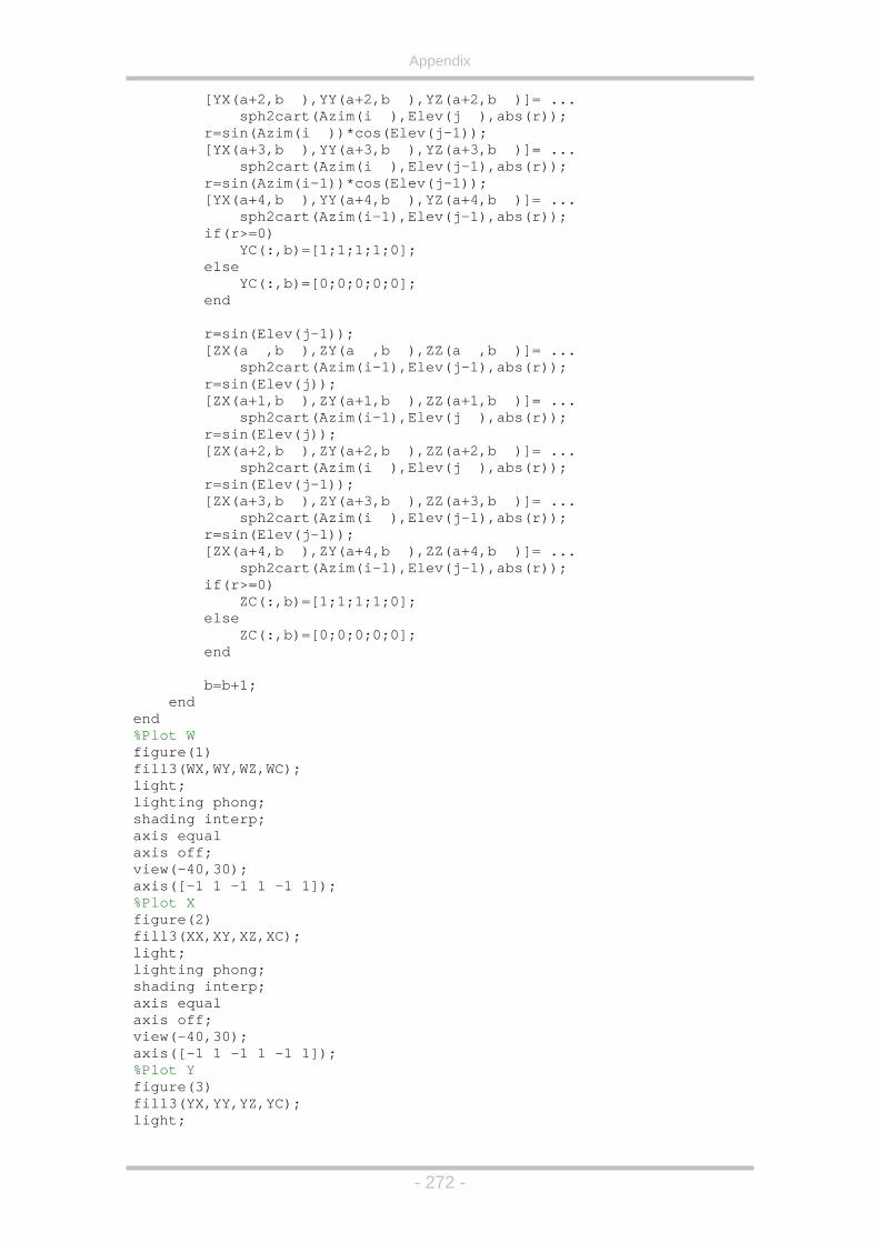
Appendix
[YX(a+2,b ),YY(a+2,b ),YZ(a+2,b )]= ... art(Azim(i ),Elev(j ),abs(r));
n(Azim(i ))*cos(Elev(j-1)); 3,b ),YY(a+3,b ),YZ(a+3,b )]= ... 2cart(Azim(i ),Elev(j-1),abs(r));
cos(Elev(j-1)); X(a+4,b ),YY(a+4,b ),YZ(a+4,b )]= ... sph2cart(Azim(i-1),Elev(j-1),abs(r));
,b)=[1;1;1;1;0];
b)=[0;0;0;0;0];
lev(j-1)); ,b ),ZZ(a ,b )]= ...
sph2cart(Azim(i-1),Elev(j-1),abs(r)); r=sin(Elev(j));
r=sin(Elev(j)); [ZX(a+2,b ),ZY(a+2,b ),ZZ(a+2,b )]= ...
sph2cart(Azim(i ),Elev(j ),abs(r)); sin(Elev(j-1));
,b ),ZY(a+3,b ),ZZ(a+3,b )]= ... 2cart(Azim(i ),Elev(j-1),abs(r));
1)); ZY(a+4,b ),ZZ(a+4,b )]= ... Azim(i-1),Elev(j-1),abs(r));
;1;1;1;0];
0];
equal
,YZ,YC);
sph2c r=si [YX(a+ sph r=sin(Azim(i-1))* [Y if(r>=0) YC(: else YC(:, end r=sin(E [ZX(a ,b ),ZY(a
[ZX(a+1,b ),ZY(a+1,b ),ZZ(a+1,b )]= ... sph2cart(Azim(i-1),Elev(j ),abs(r));
r=
[ZX(a+3ph s
r=sin(Elev(j-4,b ), [ZX(a+
sph2cart( if(r>=0)
ZC(:,b)=[1 else ZC(:,b)=[0;0;0;0; end
b=b+1; end end %Plot W figure(1)
WX,WY,WZ,WC); fill3(ght; li
lighting phong; shading interp; axis equal is off; ax
view(-40,30); axis([-1 1 -1 1 -1 1]); %Plot X figure(2) fill3(XX,XY,XZ,XC); light; lighting phong;
ing interp; shadis ax
axis off; view(-40,30); axis([-1 1 -1 1 -1 1]); %Plot Y figure(3) ll3(YX,YYfi
light;
- 272 -
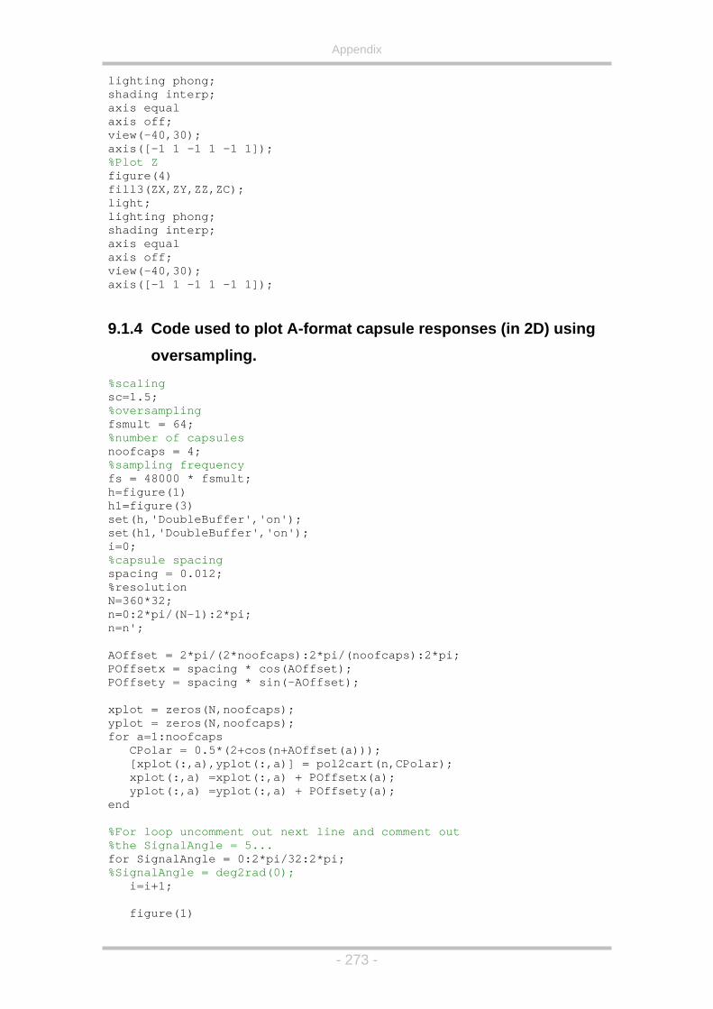
Appendix
lighting phong; shading interp; axis equal
p;
1]);
; :2*pi;
caps):2*pi/(noofcaps):2*pi; os(AOffset);
* sin(-AOffset);
=yplot(:,a) + POffsety(a);
axis off; view(-40,30); axis([-1 1 -1 1 -1 1]); %Plot Z figure(4) fill3(ZX,ZY,ZZ,ZC); light; lighting phong; shading interaxis equal axis off; view(-40,30); axis([-1 1 -1 1 -1
9.1.4 Code used to plot A-format capsule responses (in 2D) using oversampling.
%scaling sc=1.5;
rsampling %ovefsmult = 64; %number of capsules noofcaps = 4; %sampling frequency = 48000 * fsmult; fs
h=figure(1) h1=figure(3) set(h,'DoubleBuffer','on'); set(h1,'DoubleBuffer','on'); i=0; %capsule spacing spacing = 0.012;
tion %resolu0*32N=36
n=0:2*pi/(N-1)n=n'; AOffset = 2*pi/(2*noof
g * cPOffsetx = spacinpacingPOffsety = s
xplot = zeros(N,noofcaps);
ofcaps); yplot = zeros(N,nofor a=1:noofcaps CPolar = 0.5*(2+cos(n+AOffset(a))); [xplot(:,a),yplot(:,a)] = pol2cart(n,CPolar);
=xplot(:,a) + POffsetx(a); xplot(:,a)plot(:,a) y
end %For loop uncomment out next line and comment out %the SignalAngle = 5...
gle = 0:2*pi/32:2*pi; for SignalAn%SignalAngle = deg2rad(0); i=i+1; figure(1)
- 273 -

Appendix
clf hold on;
'LineWidth',1.5); alAngle) * 2;
* 2; ]);
tle('Polar Diagram of A-Format and signal direction');
inIndex = round(SignalAngle*(N-1)/(2*pi))+1; pos = 1;
noofcaps if a > noofcaps/4 & a <= 3 * noofcaps / 4
;
+ (yplot(GainIndex,a)-POffsety(a))^2); a) = (sqrt((xplot(GainIndex,a)-POffsetx(a))^2 ...
+ (yplot(GainIndex,a)-POffsety(a))^2)) * pos;
sc]);
(spacing * Gain); fs/340) + (spacing*fs/340) + 1;
); ank8 = zeros(round(2*spacing*fs/340) + 1,1);
s round(SDelay(a))) = ... nk(round(SDelay(a))) + Gain(a)/2;
FilterBank8(round(SDelay(a))) = ...
,1) Bank);
mpulses (8 imp taken from X rep)');
t(FilterBank); FilterBank/noofcaps,512*fsmult))); FilterBank8/noofcaps,512*fsmult)));
:512*fsmult/(2*fsmult))) ftarrow Omni Rep', ... ,'left');
24000,g(1:512*fsmult/(2*fsmult)),'r') *24000/255,g(x),'Figure of 8 Rep \rightarrow', ...
ignment','right');
plot(xplot,yplot, signalx = cos(Sign signaly = sin(SignalAngle) plot([signalx,0],[signaly,0 axis equal; ti Ga for a=1: pos = -1; else pos = 1; end plot(xplot(GainIndex,a),yplot(GainIndex,a),'p','LineWidth',3) Gain(a) = sqrt((xplot(GainIndex,a)-POffsetx(a))^2 ... Gain8( end axis([-sc,sc,-sc, Delay = spacing -
Delay* SDelay = ( FilterBank = zeros(round(2*spacing*fs/340) + 1,1 FilterB for a=1:noofcap FilterBank( FilterBa
FilterBank8(round(SDelay(a))) + Gain8(a)*sqrt(2); CD(a) = Delay(a); CG(a) = Gain(a); end figure(3) clf;
subplot(2,1lter stem(Fi
ylim([-4 4]); hold on; stem(FilterBank8,'r');
and Figure of 8 i title('Omni subplot(2,1,2)
nversefil invFB = i f = 20*log10(abs(fft(
*log10(abs(fft( g = 20 h = 1./f; x = 120; plot(0:24000/255:24000,f(1 text(x*24000/255,f(x),'\le
'HorizontalAlignment' hold on;
0:24000/255: plot( text(x
'HorizontalAl
- 274 -

Appendix
title('Omni and Figure of 8 responses');
too!!
f; + xplot(:,2) + xplot(:,3) + xplot(:,4))/2; + yplot(:,2) + yplot(:,3) + yplot(:,4))/2;
t(:,1) + xplot(:,2) - xplot(:,3) - xplot(:,4))*sqrt(2); (:,1) + yplot(:,2) - yplot(:,3) - yplot(:,4))*sqrt(2);
1) - xplot(:,2) - xplot(:,3) + xplot(:,4))*sqrt(2); plot(:,2) - yplot(:,3) + yplot(:,4))*sqrt(2);
Yx,Yy,'r');
ted polar diagram of B Format'); = 0.5;
-X'); ,x,'+Y');
');
reate Free Field Crosstalk Cancellation Filters
g Radius
ds (speaker is at origin, symmetry
cing));
%Left xr = xyr = y;
ylim([-20 6]); xlim([0 24000]); xlabel('Frequency (Hz)'); ylabel('Amplitude (dB)'); pause(0.1); %remember to uncomment meend figure(2) clWx = (xplot(:,1) Wy = (yplot(:,1)Xx = (xploXy = (yplotYx = (xplot(:,Yy = (yplot(:,1) - y plot(Wx,Wy); hold on plot(Xx,Xy,'m');
-Xy,'m'); plot(-Xx,plot(plot(-Yx,-Yy,'r'); axis equal; title('Reconstrucx text(x,0,'+X'); text(-x,0,'text(0text(0,-x,'-Y
9.1.5 Code Used to C%Create matlab free field dipole filters %Speakers = +/- 30 deg %Distance = 1m %Mic spacing radius = 7 cm (head radius) %Filter Size N = 1024;
Spacin%Mic MSpacing = 0.07; %Speaker spacing +/- n degrees
= 30; SSpacing%Sampling Frequency fs = 96000; %Speed of Sound in Air c = 342; %Middle of Head x & y co-or%assumed) x = sin(deg2rad(SSpay = cos(deg2rad(SSpacing));
and Right Mic Coords - MSpacing;
xl = x + MSpacing;
- 275 -

Appendix
yl = y; %Calculate Distances from origin (speaker)
ference at mics using inverse square law
e using speed of sound ime = rdist/c;
ime; to number of samples
reate filters
1 a) = 1;
ount=count+2; ound(a/(sampdif*2))==a/(sampdif*2)
h1(a+1) = ADif^count;
ampdif+1); = -ADif;
=conv(h1,ht);
Domain Representation
ld on r'); eWidth',2); idth',2); alk filters at +/- ',num2str(SSpacing),' degrees']); ',' ','h2',' '); itude');
abel('Sample Number (at 96kHz, c = 342ms-1)');
sentation
ineWidth',2);
,1024))),'r:','LineWidth',2);
esponse at +/- ',num2str(SSpacing),' degrees']); (Hz)'); (dB)');
alk Cancellation Filters Using ring Techniques
hrtf\ofull\elev0\';
rdist = sqrt(xr*xr + yr*yr); ldist = sqrt(xl*xl + yl*yl); %Calculate Amplitude difADif = 1-(ldist-rdist); %Convert distance to timrtltime = ldist/c; timedif = ltime - rt%Convert time sampdif = round(timedif * fs); %Ch1=zeros(1,N); count=1; for a=1:N
a== if h1( c elseif r count=count+2; end end ht = zeros(1,sht(sampdif+1) h2
Time%Plot figure(1) clf; a=stem(h1); hob=stem(h2,'
'Linset(a,set(b,'LineWtitle(['x-t
('h1legendylabel('Amplxlaxis([0 1024 -1.05 1.05]); %Plot Frequency Domain Resprefigure(2) clf; freq=0:fs/(N-1):fs; plot(freq,20*log10(abs(fft(h1))),'Lhold on plot(freq,20*log10(abs(fft(h2xlim([0 fs/4]); title(['Frequency Rxlabel('Frequencyylabel('Amplitude legend('h1','h2');
9.1.6 Code Used to Create CrosstHRTF Data and Inverse Filte
pinna = 1; d = 'd:\matlab\
- 276 -

Appendix
ref = wavread([d, 'L0e175a.wav']); pinna); ([d, 'L0e185a.wav']);
d, 'L0e175a.wav']); tfR = hrtf(:,pinna);
L;
win=hanning(len); iL=iL.*win'; figure(5) clf; plot(iL); hold on plot(win); L2 = conv(hrtfL,iL); R2 = conv(hrtfR,iL); win=hanning(length(L2));
figure(1) clf; plot(L2); hold on plot(R2,'r'); figure(2) clf; freqz(L2); figure(3) clf; freqz(R2); [h1,h2] = freqdip([L2'],[R2'],len,0,0); h1inv = inversefilt(h1,0.0); h1i = conv(h1,h1inv); h2i = conv(h2,h1inv); h1i = h1i((len-1024):(len+1023)); h2i = h2i((len-1024):(len+1023)); win = hanning(length(h1i)); h1i = h1i .* win; h2i = h2i .* win; figure(6) plot([h1i,h2i]); h1i48 = resample(h1i,48000,44100); h2i48 = resample(h2i,48000,44100); h148 = resample(h1,48000,44100); h248 = resample(h2,48000,44100); %Carry out test dipole simulation %c = wavread('h0e030a.wav'); %c1 = c(:,2);
refR = ref(:,ref = wavreadrefL = ref(:,pinna); hrtf = wavread([hrhrtf = wavread([d, 'L0e185a.wav']); hrtfL = hrtf(:,pinna); len=4096; temp=zeros(1,len); offset=2048; mp(offset:offset-1+length(hrtfL))=refte
iL=inversefilt(temp);
L2=L2.*win'; R2=R2.*win';
- 277 -

Appendix
%c2 = c(:,1); c1 = hrtfL; c2 = hrtfR; source=zeros(8191,2); source(1,1)=1; dipolesig=[conv(source(:,1),h1i)+conv(source(:,2),h2i),conv(source(:,2),h1i)+conv(source(:,1),h2i)]; leftspeakerl=conv(dipolesig(:,1),c1); leftspeakerr=conv(dipolesig(:,1),c2); rightspeakerl=conv(dipolesig(:,2),c2); rightspeakerr=conv(dipolesig(:,2),c1); stereoout=[leftspeakerl+rightspeakerl,leftspeakerr+rightspeakerr]; figure(7) clf; freqz(stereoout(:,1));
freqz(stereoout(:,2));
9.1.7 Matlab Code Used in FreqDip Function for the Generation of Crosstalk Cancellation Filters
function [h1,h2]=freqdip(tc1,tc2,FiltLength,inband,outband) %[h1,h2]=freqdip(tc1,tc2,FiltLength,inband,outband) % Frequency Domain XTalk Cancellation Filters Lf = 500; Hf = 20000; if(nargin<3) FiltLength=2048; inband=0.0002; outband=1; elseif(nargin<5)
outband=1; end LowerFreq=round(FiltLength*Lf/22050); UpperFreq=round(FiltLength*Hf/22050); reg=ones(FiltLength,1); reg(1:LowerFreq) = outband; reg(LowerFreq:UpperFreq) = inband; reg(UpperFreq:FiltLength)= outband; regx=0:22051/FiltLength:22050; figure(1) clf plot(regx,reg); c1=tc1; c2=tc2; fc1=fft(c1,FiltLength); fc2=fft(c2,FiltLength); fnc2=fft(-c2,FiltLength); Filt=(fc1.*fc1)-(fc2.*fc2); FiltDenom=1./Filt; fh1=fc1.*FiltDenom; fh2=fnc2.*FiltDenom;
hold on
inband=0.0002;
- 278 -

Appendix
- 279 -
w = hanning(FiltLength); h1=real(ifft(fh1,FiltLength)) .* w; h2=real(ifft(fh2,FiltLength)) .* w; figure(2) clf; plot(h1) hold on plot(h2,'r'); figure(3) clf freqz(h1,1,length(h1),44100) hold on freqz(h2,1,length(h2),44100) %Carry out test dipole simulation source=zeros(1024,2); source(1,1)=1; dipolesig=[conv(source(:,1),h1)+conv(source(:,2),h2),conv(source(:,2),h1)+conv(source(:,1),h2)]; leftspeakerl=conv(dipolesig(:,1),c1); leftspeakerr=conv(dipolesig(:,1),c2); rightspeakerl=conv(dipolesig(:,2),c2); rightspeakerr=conv(dipolesig(:,2),c1); stereoout=[leftspeakerl+rightspeakerl,leftspeakerr+rightspeakerr]; figure(4) plot(stereoout);
9.1.8 Matlab Code Used To Generate Inverse Filters function res = inversefilt(signal,mix) %RES = INVERSEFILT(SIGNAL) if(nargin==1) mix = 1; end fftsize=2^(ceil(log2(length(signal)))); fsignal=fft(signal,fftsize); mag = abs(fsignal); ang = angle(fsignal); newmag = 1./mag; newang = -ang; newfsignal = newmag.*exp(i*newang); newsignal = real(ifft(newfsignal,fftsize)); if(nargin==1) res = newsignal(1:length(signal)); else out = newsignal(1:length(signal)); a = grpdelay(out,1,fftsize); b = round(sum(a)/fftsize); sig = zeros(size(out)); sig(b) = 1;

Appendix
- 280 -
fo = fft(out); fm = fft(sig); fomag = abs(fo); fmmag = abs(fm); foang = angle(fo); fmang = angle(fm); newmag = (mix * fomag) + ((1-mix) * fmmag); newang = fmang; newfft = newmag.*exp(i*newang); fres = ifft(newfft,fftsize); res = real(fres); res = res(1:length(signal)); end
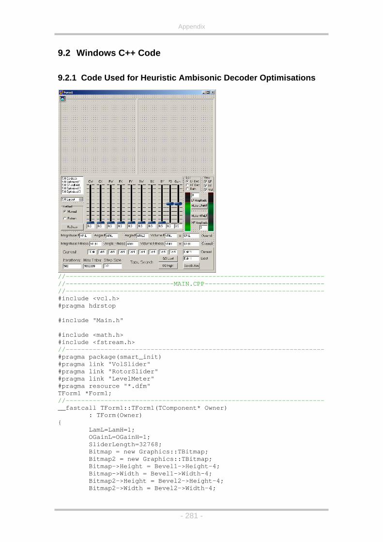
Appendix
9.2 Windows C++ Code
9.2.1 Code Used for Heuristic Ambisonic Decoder Optimisations
#pragma hdrstop
//------------------------------------------------------------------- //----------------------------MAIN.CPP------------------------------- //------------------------------------------------------------------- #include <vcl.h>
#include "Main.h" #include <math.h> #include <fstream.h> //------------------------------------------------------------------- #pragma package(smart_init) #pragma link "VolSlider" #pragma link "RotorSlider" #pragma link "LevelMeter" #pragma resource "*.dfm" TForm1 *Form1; //------------------------------------------------------------------- __fastcall TForm1::TForm1(TComponent* Owner) : TForm(Owner) { LamL=LamH=1; OGainL=OGainH=1; SliderLength=32768; Bitmap = new Graphics::TBitmap; Bitmap2 = new Graphics::TBitmap; Bitmap->Height = Bevel1->Height-4; Bitmap->Width = Bevel1->Width-4; Bitmap2->Height = Bevel2->Height-4; Bitmap2->Width = Bevel2->Width-4;
- 281 -

Appendix
- 282 -
MaxX = Bitmap->Width/2; MaxY = Bitmap->Height/2; NoOfSpeakers = 5; SpeakPos[0] = 0; SpeakPos[1] = Deg2Rad(30); SpeakPos[2] = Deg2Rad(115); SpeakPos[3] = Deg2Rad(-115); SpeakPos[4] = Deg2Rad(-30); ListBox1->ItemIndex=0; ListBox1Click(this); WGain[0] = WGainH[0] =
(double)VolSlider1->Position/SliderLength; WGain[1] = WGainH[1] =
(double)VolSlider3->Position/SliderLength; WGain[2] = WGainH[2] =
(double)VolSlider6->Position/SliderLength; XGain[0] = XGainH[0] =
(double)VolSlider2->Position/SliderLength; XGain[1] = XGainH[1] =
(double)VolSlider4->Position/SliderLength; XGain[2] = XGainH[2] =
-(double)VolSlider7->Position/SliderLength; YGain[1] = YGainH[1] =
(double)VolSlider5->Position/SliderLength; YGain[2] = YGainH[2] =
(double)VolSlider8->Position/SliderLength; RadioGroup1->ItemIndex=1; VolSlider1Change(this); RadioGroup1->ItemIndex=0; VolSlider1Change(this); } //------------------------------------------------------------------- double TForm1::Deg2Rad(double Deg) { return (Deg*M_PI/180); } //------------------------------------------------------------------- void TForm1::GPaint() { long a,b,c,d; int SpRad = 5; Bitmap->Canvas->Pen->Style = psDot; Bitmap->Canvas->Pen->Color = clBlack; Bitmap->Canvas->Brush->Style = bsSolid; Bitmap->Canvas->Brush->Color = clWhite; Bitmap->Canvas->Rectangle(0,0,Bitmap->Width,Bitmap->Height); Bitmap->Canvas->Ellipse(0,0,Bitmap->Width,Bitmap->Height); Bitmap->Canvas->Pen->Style = psSolid; Bitmap->Canvas->Brush->Style = bsSolid; Bitmap->Canvas->Brush->Color = clBlue; for(int i=0;i<NoOfSpeakers;i++) { double x,y; int r = MaxY - 10; x = r * cos(SpeakPos[i]) + MaxX; y = r * sin(SpeakPos[i]) + MaxY; Bitmap->Canvas->Rectangle(
x-SpRad,y-SpRad,x+SpRad,y+SpRad); } double r8 = 0.35355339059327376220042218105242; double r2 = 0.70710678118654752440084436210485; double MFitnessL=0,AFitnessL=0,OFitnessL=0,VFitnessL=0,Ang;

Appendix
- 283 -
double MFitnessH=0,AFitnessH=0,OFitnessH=0,VFitnessH=0; for(int i=0;i<360;i++) { double Rad = Deg2Rad(i); WSig = 1/sqrt(2); XSig = cos(Rad); YSig = sin(Rad); WSigL = (0.5*(LamL+ILamL)*WSig) +
(r8*(LamL-ILamL)*XSig); XSigL = (0.5*(LamL+ILamL)*XSig) +
(r2*(LamL-ILamL)*WSig); YSigL = YSig; WSigH = (0.5*(LamH+ILamH)*WSig) +
(r8*(LamH-ILamH)*XSig); XSigH = (0.5*(LamH+ILamH)*XSig) +
(r2*(LamH-ILamH)*WSig); YSigH = YSig; SpGain[0] = (WGain[0]*WSigL + XGain[0]*XSigL); SpGain[1] = (WGain[1]*WSigL + XGain[1]*XSigL +
YGain[1]*YSigL); SpGain[2] = (WGain[2]*WSigL + XGain[2]*XSigL +
YGain[2]*YSigL); SpGain[3] = (WGain[2]*WSigL + XGain[2]*XSigL -
YGain[2]*YSigL); SpGain[4] = (WGain[1]*WSigL + XGain[1]*XSigL –
YGain[1]*YSigL); SpGainH[0] = (WGainH[0]*WSigH + XGainH[0]*XSigH); SpGainH[1] = (WGainH[1]*WSigH + XGainH[1]*XSigH +
YGainH[1]*YSigH); SpGainH[2] = (WGainH[2]*WSigH + XGainH[2]*XSigH +
YGainH[2]*YSigH); SpGainH[3] = (WGainH[2]*WSigH + XGainH[2]*XSigH –
YGainH[2]*YSigH); SpGainH[4] = (WGainH[1]*WSigH + XGainH[1]*XSigH –
YGainH[1]*YSigH); P=P2=E=VecLowX=VecLowY=VecHighX=VecHighY=0; for(int j=0;j<NoOfSpeakers;j++) { P+=SpGain[j]; P2+=SpGainH[j]*SpGainH[j]; E+=pow(SpGainH[j],2); } VolLx[i]=(P*cos(Rad)*MaxX/5)+MaxX; VolLy[i]=(P*sin(Rad)*MaxY/5)+MaxY; VolHx[i]=(P2*cos(Rad)*MaxX/5)+MaxX; VolHy[i]=(P2*sin(Rad)*MaxY/5)+MaxY; if(i==0) { LFVol = P/NoOfSpeakers; HFVol = P2/NoOfSpeakers; } for(int j=0;j<NoOfSpeakers;j++) { VecLowX+=SpGain[j]*cos(SpeakPos[j]); VecLowY+=SpGain[j]*sin(SpeakPos[j]); VecHighX+=pow(SpGainH[j],2)*cos(SpeakPos[j]); VecHighY+=pow(SpGainH[j],2)*sin(SpeakPos[j]); } if(P && E) {
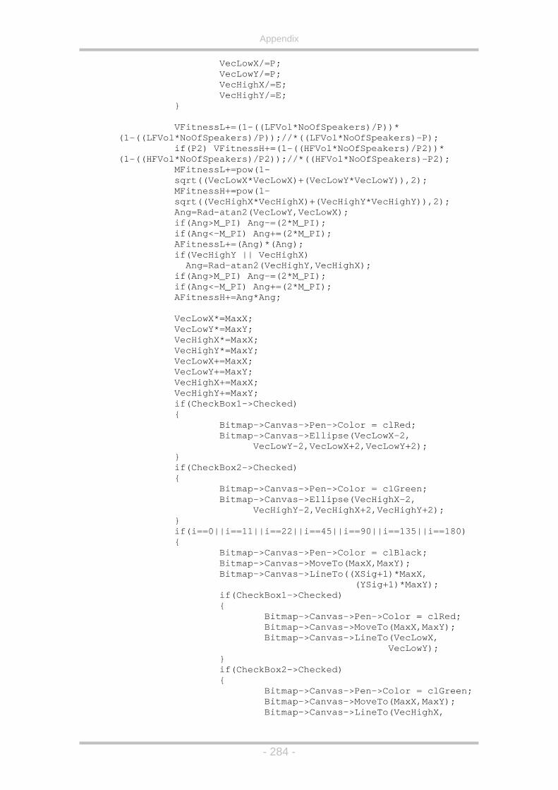
Appendix
VecLowX/=P; VecLowY/=P; VecHighX/=E; VecHighY/=E; } VFitnessL+=(1-((LFVol*NoOfSpeakers)/P))*
(1-((LFVol*NoOfSpeakers)/P));//*((LFVol*NoOfSpeakers)-P); if(P2) VFitnessH+=(1-((HFVol*NoOfSpeakers)/P2))*
(1-((HFVol*NoOfSpeakers)/P2));//*((HFVol*NoOfSpeakers)-P2); MFitnessL+=pow(1-
sqrt((VecLowX*VecLowX)+(VecLowY*VecLowY)),2); MFitnessH+=pow(1-
sqrt((VecHighX*VecHighX)+(VecHighY*VecHighY)),2); Ang=Rad-atan2(VecLowY,VecLowX); if(Ang>M_PI) Ang-=(2*M_PI); if(Ang<-M_PI) Ang+=(2*M_PI); AFitnessL+=(Ang)*(Ang); if(VecHighY || VecHighX)
Ang=Rad-atan2(VecHighY,VecHighX); if(Ang>M_PI) Ang-=(2*M_PI); if(Ang<-M_PI) Ang+=(2*M_PI); AFitnessH+=Ang*Ang; VecLowX*=MaxX; VecLowY*=MaxY; VecHighX*=MaxX; VecHighY*=MaxY; VecLowX+=MaxX; VecLowY+=MaxY; VecHighX+=MaxX; VecHighY+=MaxY; if(CheckBox1->Checked) { Bitmap->Canvas->Pen->Color = clRed; Bitmap->Canvas->Ellipse(VecLowX-2,
VecLowY-2,VecLowX+2,VecLowY+2); } if(CheckBox2->Checked) { Bitmap->Canvas->Pen->Color = clGreen; Bitmap->Canvas->Ellipse(VecHighX-2,
VecHighY-2,VecHighX+2,VecHighY+2); } if(i==0||i==11||i==22||i==45||i==90||i==135||i==180) { Bitmap->Canvas->Pen->Color = clBlack; Bitmap->Canvas->MoveTo(MaxX,MaxY); Bitmap->Canvas->LineTo((XSig+1)*MaxX,
(YSig+1)*MaxY); if(CheckBox1->Checked) { Bitmap->Canvas->Pen->Color = clRed; Bitmap->Canvas->MoveTo(MaxX,MaxY); Bitmap->Canvas->LineTo(VecLowX,
VecLowY); } if(CheckBox2->Checked) { Bitmap->Canvas->Pen->Color = clGreen; Bitmap->Canvas->MoveTo(MaxX,MaxY); Bitmap->Canvas->LineTo(VecHighX,
- 284 -

Appendix
- 285 -
VecHighY); } } } if(CheckBox3->Checked) { int Div=5; Bitmap->Canvas->Pen->Color=clRed; Bitmap->Canvas->MoveTo((int)VolLx[359],
(int)VolLy[359]); for(int a=0;a<360;a++) { Bitmap->Canvas->LineTo((int)VolLx[a],
(int)VolLy[a]); } Bitmap->Canvas->MoveTo(
(int)((VolLx[359]-MaxX)/Div)+MaxX, (int)((VolLy[359]-MaxY)/Div)+MaxY);
for(int a=0;a<360;a++) { Bitmap->Canvas->LineTo(
(int)((VolLx[a]-MaxX)/Div)+MaxX, (int)((VolLy[a]-MaxY)/Div)+MaxY);
} Bitmap->Canvas->Pen->Color=clGreen; Bitmap->Canvas->MoveTo((int)VolHx[359],
(int)VolHy[359]); for(int a=0;a<360;a++) { Bitmap->Canvas->LineTo((int)VolHx[a],
(int)VolHy[a]); } } VFitnessL=sqrt(VFitnessL/360.0f); VFitnessH=sqrt(VFitnessH/360.0f); AFitnessL=sqrt(AFitnessL/360.0f); AFitnessH=sqrt(AFitnessH/360.0f); MFitnessL=sqrt(MFitnessL/360.0f); MFitnessH=sqrt(MFitnessH/360.0f); OFitnessL=VFitnessL + AFitnessL + MFitnessL; OFitnessH=VFitnessH + AFitnessH + MFitnessH; a = Bevel1->Left + 2; b = Bevel1->Top + 2; c = Bevel1->Width + a -2; d = Bevel1->Height + b -2; BitBlt(Form1->Canvas->Handle,a,b,c,d,
Bitmap->Canvas->Handle,0,0,SRCCOPY); MFitL->Text=FloatToStrF(MFitnessL,ffFixed,5,5); MFitH->Text=FloatToStrF(MFitnessH,ffFixed,5,5); AFitL->Text=FloatToStrF(AFitnessL,ffFixed,5,5); AFitL2->Text=FloatToStrF(AFitnessL,ffFixed,5,5); AFitH->Text=FloatToStrF(AFitnessH,ffFixed,5,5); VFitL->Text=FloatToStrF(VFitnessL,ffFixed,5,5); VFitH->Text=FloatToStrF(VFitnessH,ffFixed,5,5); OFitL->Text=FloatToStrF(OFitnessL,ffFixed,5,5); OFitH->Text=FloatToStrF(OFitnessH,ffFixed,5,5); LFEdit->Text=FloatToStrF(LFVol,ffFixed,3,3); HFEdit->Text=FloatToStrF(HFVol,ffFixed,3,3); LevelMeter1->MeterReading=(int)(LFVol*75); LevelMeter2->MeterReading=(int)(HFVol*75); } //-------------------------------------------------------------------

Appendix
void TForm1::RPaint() { long a,b,c,d; int skip = 9; Bitmap2->Canvas->Pen->Style = psDot; Bitmap2->Canvas->Pen->Color = clBlack;
Bitmap2->Canvas->Rectangle(0,0, Bitmap2->Width,Bitmap2->Height);
for(int i=0;i<360;i+=skip) {
Rep1[i] = 0.5 * (0.7071 * WGain[0] + cos(Deg2Rad(i))*XGain[0]);
Rep2[i] = 0.5 * (0.7071 * WGain[1] + cos(Deg2Rad(i))*XGain[1] + sin(Deg2Rad(i))*YGain[1]);
Rep4[i] = 0.5 * (0.7071 * WGain[2] + cos(Deg2Rad(i))*XGain[2] - sin(Deg2Rad(i))*YGain[2]);
Rep5[i] = 0.5 * (0.7071 * WGain[1] + cos(Deg2Rad(i))*XGain[1] - sin(Deg2Rad(i))*YGain[1]);
Rep1[i]<0?Rep1[i]=-Rep1[i]:Rep1[i]=Rep1[i]; Rep2[i]<0?Rep2[i]=-Rep2[i]:Rep2[i]=Rep2[i]; Rep3[i]<0?Rep3[i]=-Rep3[i]:Rep3[i]=Rep3[i]; Rep4[i]<0?Rep4[i]=-Rep4[i]:Rep4[i]=Rep4[i]; Rep5[i]<0?Rep5[i]=-Rep5[i]:Rep5[i]=Rep5[i]; } else { Rep1[i] = 0.5 * (0.7071 * WGainH[0] +
cos(Deg2Rad(i))*XGainH[0]); Rep2[i] = 0.5 * (0.7071 * WGainH[1] +
cos(Deg2Rad(i))*XGainH[1] + sin(Deg2Rad(i))*YGainH[1]); Rep3[i] = 0.5 * (0.7071 * WGainH[2] +
cos(Deg2Rad(i))*XGainH[2] + sin(Deg2Rad(i))*YGainH[2]); Rep4[i] = 0.5 * (0.7071 * WGainH[2] +
cos(Deg2Rad(i))*XGainH[2] - sin(Deg2Rad(i))*YGainH[2]); Rep5[i] = 0.5 * (0.7071 * WGainH[1] +
cos(Deg2Rad(i))*XGainH[1] - sin(Deg2Rad(i))*YGainH[1]); Rep1[i]<0?Rep1[i]=-Rep1[i]:Rep1[i]=Rep1[i]; Rep2[i]<0?Rep2[i]=-Rep2[i]:Rep2[i]=Rep2[i]; Rep3[i]<0?Rep3[i]=-Rep3[i]:Rep3[i]=Rep3[i]; Rep4[i]<0?Rep4[i]=-Rep4[i]:Rep4[i]=Rep4[i]; Rep5[i]<0?Rep5[i]=-Rep5[i]:Rep5[i]=Rep5[i]; } } Bitmap2->Canvas->Pen->Width = 2; Bitmap2->Canvas->Pen->Style=psSolid; Bitmap2->Canvas->Pen->Color=clBlack; PlotPolar(Bitmap2,Rep1,skip); Bitmap2->Canvas->Pen->Color=clRed; PlotPolar(Bitmap2,Rep2,skip); Bitmap2->Canvas->Pen->Color=clBlue; PlotPolar(Bitmap2,Rep3,skip); Bitmap2->Canvas->Pen->Color=clPurple; PlotPolar(Bitmap2,Rep4,skip); Bitmap2->Canvas->Pen->Color=clTeal; PlotPolar(Bitmap2,Rep5,skip); a = Bevel2->Left + 2;
Bitmap2->Canvas->Brush->Style = bsSolid; Bitmap2->Canvas->Brush->Color = clWhite;
if(RadioGroup1->ItemIndex==0) {
Rep3[i] = 0.5 * (0.7071 * WGain[2] + cos(Deg2Rad(i))*XGain[2] + sin(Deg2Rad(i))*YGain[2]);
- 286 -

Appendix
b = Bevel2->Top + 2; c = Bevel2->Width + a -2; d = Bevel2->Height + b -2; BitBlt(Form1->Canvas->Handle,a,b,c,d,
Bitmap2->Canvas->Handle,0,0,SRCCOPY); } //------------------------------------------------------------------- void __fastcall TForm1::Button1Click(TObject *Sender) { GPaint(); RPaint(); } //------------------------------------------------------------------- void __fastcall TForm1::FormPaint(TObject *Sender) { GPaint(); RPaint(); } //------------------------------------------------------------------- void __fastcall TForm1::VolSlider1Change(TObject *Sender) { if(RadioGroup1->ItemIndex==0) { OGainL =
(double)VolSlider10->Position*2/SliderLength; WGain[0] =
(double)OGainL*VolSlider1->Position/SliderLength; WGain[1] =
(double)OGainL*VolSlider3->Position/SliderLength; WGain[2] =
(double)OGainL*VolSlider6->Position/SliderLength; XGain[0] =
(double)OGainL*VolSlider2->Position/SliderLength; XGain[1] =
(double)OGainL*VolSlider4->Position/SliderLength; XGain[2] =
-(double)OGainL*VolSlider7->Position/SliderLength; YGain[1] =
(double)OGainL*VolSlider5->Position/SliderLength; YGain[2] =
(double)OGainL*VolSlider8->Position/SliderLength; LamL =
if(LamL) ILamL=1/LamL; } else if(RadioGroup1->ItemIndex==1) { WGainH[0] =
(double)OGainH*VolSlider1->Position/SliderLength; WGainH[1] =
(double)OGainH*VolSlider3->Position/SliderLength; WGainH[2] =
(double)OGainH*VolSlider6->Position/SliderLength; XGainH[0] =
(double)OGainH*VolSlider2->Position/SliderLength; XGainH[1] =
(double)OGainH*VolSlider4->Position/SliderLength; XGainH[2] =
-(double)OGainH*VolSlider7->Position/SliderLength;
(double)VolSlider9->Position*2/SliderLength;
- 287 -

Appendix
YGainH[1] = (double)OGainH*VolSlider5->Position/SliderLength;
YGainH[2] = (double)OGainH*VolSlider8->Position/SliderLength;
LamH = (double)VolSlider9->Position*2/SliderLength;
if(LamH) ILamH=1/LamH; OGainH =
(double)VolSlider10->Position*2/SliderLength; } else if(RadioGroup1->ItemIndex==2) { OGainH = OGainL =
(double)VolSlider10->Position*2/SliderLength; WGainH[0] = WGain[0] =
(double)OGainL*VolSlider1->Position/SliderLength; WGainH[1] = WGain[1] =
(double)OGainL*VolSlider3->Position/SliderLength; WGainH[2] = WGain[2] =
(double)OGainL*VolSlider6->Position/SliderLength; XGainH[0] = XGain[0] =
(double)OGainL*VolSlider2->Position/SliderLength; XGainH[1] = XGain[1] =
(double)OGainL*VolSlider4->Position/SliderLength; XGainH[2] = XGain[2] = -
YGainH[1] = YGain[1] = (double)OGainL*VolSlider5->Position/SliderLength;
YGainH[2] = YGain[2] = (double)OGainL*VolSlider8->Position/SliderLength;
LamH = LamL = (double)VolSlider9->Position*2/SliderLength;
if(LamL) ILamL=1/LamL; if(LamH) ILamH=1/LamH; } UpdateEdits(); GPaint(); RPaint(); } //------------------------------------------------------------------- void TForm1::UpdateEdits() { if(RadioGroup1->ItemIndex==0) { Edit1->Text=FloatToStrF(WGain[0],
ffFixed,3,3); Edit3->Text=FloatToStrF(WGain[1],
ffFixed,3,3); Edit6->Text=FloatToStrF(WGain[2],
ffFixed,3,3); Edit2->Text=FloatToStrF(XGain[0],
ffFixed,3,3); Edit4->Text=FloatToStrF(XGain[1],
ffFixed,3,3); Edit7->Text=FloatToStrF(XGain[2],
ffFixed,3,3); Edit5->Text=FloatToStrF(YGain[1],
ffFixed,3,3);
(double)OGainL*VolSlider7->Position/SliderLength;
- 288 -

Appendix
Edit8->Text=FloatToStrF(YGain[2], ffFixed,3,3);
Edit9->Text=FloatToStrF(LamL,ffFixed,3,3); Edit10->Text=FloatToStrF(OGainL,ffFixed,3,3); } else if(RadioGroup1->ItemIndex==1) { Edit1->Text=FloatToStrF(WGainH[0],
ffFixed,3,3); Edit3->Text=FloatToStrF(WGainH[1],
ffFixed,3,3);
ffFixed,3,3); Edit2->Text=FloatToStrF(XGainH[0],
ffFixed,3,3); Edit4->Text=FloatToStrF(XGainH[1],
ffFixed,3,3); Edit7->Text=FloatToStrF(XGainH[2],
ffFixed,3,3); Edit5->Text=FloatToStrF(YGainH[1],
ffFixed,3,3); Edit8->Text=FloatToStrF(YGainH[2],
ffFixed,3,3); Edit9->Text=FloatToStrF(LamH,ffFixed,3,3); Edit10-
Edit6->Text=FloatToStrF(WGainH[2],
>Text=FloatToStrF(OGainH,ffFixed,3,3); } } //------------------------------------------------------------------- void TForm1::UpdateNewEdits() { if(RadioGroup1->ItemIndex==0) { GEdit1->Text=FloatToStrF(
(float)GainSlider1->Position/100,ffFixed,3,3); GEdit2->Text=FloatToStrF(
(float)GainSlider2->Position/100,ffFixed,3,3); GEdit3->Text=FloatToStrF(
(float)GainSlider3->Position/100,ffFixed,3,3); DEdit1->Text=FloatToStrF(
(float)DSlider1->Position/100,ffFixed,3,3); DEdit2->Text=FloatToStrF(
(float)DSlider2->Position/100,ffFixed,3,3); DEdit3->Text=FloatToStrF(
(float)DSlider3->Position/100,ffFixed,3,3); AEdit1->Text=IntToStr(
(int)ASlider1->DotPosition); AEdit2->Text=IntToStr(
(int)ASlider2->DotPosition); AEdit3->Text=IntToStr(
(int)ASlider3->DotPosition); } else if(RadioGroup1->ItemIndex==1) { GEdit1->Text=FloatToStrF(
(float)GainSlider1->Position/100,ffFixed,3,3); GEdit2->Text=FloatToStrF(
(float)GainSlider2->Position/100,ffFixed,3,3); GEdit3->Text=FloatToStrF(
(float)GainSlider3->Position/100,ffFixed,3,3); DEdit1->Text=FloatToStrF(
(float)DSlider1->Position/100,ffFixed,3,3); DEdit2->Text=FloatToStrF(
- 289 -

Appendix
- 290 -
(float)DSlider2->Position/100,ffFixed,3,3); DEdit3->Text=FloatToStrF(
(float)DSlider3->Position/100,ffFixed,3,3); AEdit1->Text=FloatToStrF(
(float)ASlider1->DotPosition/100,ffFixed,3,3); AEdit2->Text=FloatToStrF(
(float)ASlider2->DotPosition/100,ffFixed,3,3); AEdit3->Text=FloatToStrF(
(float)ASlider3->DotPosition/100,ffFixed,3,3); }
} //------------------------------------------------------------------- void __fastcall TForm1::ListBox1Click(TObject *Sender) { if(ListBox1->ItemIndex==0) { VolSlider1->Position = 0.34190f*SliderLength; VolSlider3->Position = 0.26813f*SliderLength; VolSlider6->Position = 0.56092f*SliderLength; VolSlider2->Position = 0.23322f*SliderLength; VolSlider4->Position = 0.38191f*SliderLength; VolSlider7->Position = 0.49852f*SliderLength; VolSlider5->Position = 0.50527f*SliderLength; VolSlider8->Position = 0.45666f*SliderLength; VolSlider9->Position = 1*SliderLength/2; VolSlider10->Position = 1*SliderLength/2; VolSlider1Change(this); WGainH[0]=0.38324f; WGainH[1]=0.44022f; WGainH[2]=0.78238f; XGainH[0]=0.37228f; XGainH[1]=0.23386f; XGainH[2]=-0.55322f; YGainH[1]=0.54094f; YGainH[2]=0.42374f; LamH=1; ILamH=1/LamH; OGainH=1; } else if(ListBox1->ItemIndex==1) { RadioGroup1->ItemIndex=0; VolSlider1->Position = 0.58*SliderLength; VolSlider3->Position = 0.16*SliderLength; VolSlider6->Position = 1*SliderLength; VolSlider2->Position = 0.47*SliderLength; VolSlider4->Position = 0.53*SliderLength;
VolSlider7->Position = 0.77*SliderLength; VolSlider5->Position = 0.55*SliderLength;
VolSlider8->Position = 0.83*SliderLength; VolSlider9->Position = 1*SliderLength/2; VolSlider10->Position = 1*SliderLength/2; VolSlider1Change(this); WGainH[0]=0.260; WGainH[1]=0.320; WGainH[2]=1.000; XGainH[0]=0.200; XGainH[1]=0.280; XGainH[2]=-0.64; YGainH[1]=0.480;
Appendix
YGainH[2]=0.340; LamH=1; ILamH=1/LamH; OGainH=1; } else if(ListBox1->ItemIndex==2) { RadioGroup1->ItemIndex=0; VolSlider1->Position = sqrt(2.0f)*SliderLength; VolSlider3->Position = sqrt(2.0f)*SliderLength; VolSlider6->Position = sqrt(2.0f)*SliderLength; VolSlider2->Position = cos(SpeakPos[0])*SliderLength; VolSlider4->Position = cos(Deg2Rad(45))*SliderLength; VolSlider7->Position = -cos(Deg2Rad(135))
*SliderLength; VolSlider5->Position = sin(Deg2Rad(45))*SliderLength; VolSlider8->Position = sin(Deg2Rad(135))
*SliderLength; VolSlider9->Position = 1*SliderLength/2; VolSlider10->Position = 1*SliderLength/2; VolSlider1Change(this); WGainH[0]=WGain[0]; WGainH[1]=WGain[1]; WGainH[2]=WGain[2]; XGainH[0]=XGain[0]; XGainH[1]=XGain[1]; XGainH[2]=XGain[2];
YGainH[2]=YGain[2]; LamH=1; ILamH=1/LamH; OGainH=1;
else if(ListBox1->ItemIndex==3) { RadioGroup1->ItemIndex=0; VolSlider1->Position = 0.023*SliderLength; VolSlider3->Position = 0.4232*SliderLength; VolSlider6->Position = 0.9027*SliderLength; VolSlider2->Position = 0.2518*SliderLength; VolSlider4->Position = 0.6014*SliderLength; VolSlider7->Position = 0.7245*SliderLength; VolSlider5->Position = 0.2518*SliderLength; VolSlider8->Position = 0.9062*SliderLength; VolSlider9->Position = 1*SliderLength/2; VolSlider10->Position = 1*SliderLength/2; VolSlider1Change(this);
WGainH[1]=0.6086; WGainH[2]=1.0290; XGainH[0]=0; XGainH[1]=0.4998; XGainH[2]=-0.2058; YGainH[1]=0.3861; YGainH[2]=0.2489; LamH=0.9270; ILamH=1/LamH; OGainH=1; } else if(ListBox1->ItemIndex==4) { RadioGroup1->ItemIndex=0;
YGainH[1]=YGain[1];
}
WGainH[0]=0;
- 291 -

Appendix
VolSlider1->Position = 0.26*SliderLength; VolSlider3->Position = 0.34*SliderLength; VolSlider6->Position = 1*SliderLength; VolSlider2->Position = 0.247*SliderLength; VolSlider4->Position = 0.66*SliderLength; VolSlider7->Position = 0.78*SliderLength; VolSlider5->Position = 1*SliderLength; VolSlider8->Position = 0.587*SliderLength; VolSlider9->Position = 1*SliderLength/2; VolSlider10->Position = 1*SliderLength/2; VolSlider1Change(this); WGainH[0]=0.312; WGainH[1]=0.503; WGainH[2]=0.868; XGainH[0]=0.176; XGainH[1]=0.563; XGainH[2]=-0.41; YGainH[1]=0.517;
LamH=1.030; ILamH=1/LamH; OGainH=1; } GPaint(); RPaint(); } //------------------------------------------------------------------- void __fastcall TForm1::CheckBox1Click(TObject *Sender) { VolSlider1Change(this); } //-------------------------------------------------------------------void TForm1::PlotPolar(Graphics::TBitmap *Bmap,double *Radius,
int skip) { int t1,t2; t1=(int)(Radius[360-skip]*cos(Deg2Rad(360-skip))*MaxX)+MaxX; t2=(int)(Radius[360-skip]*sin(Deg2Rad(360-skip))*MaxY)+MaxY; Bmap->Canvas->MoveTo(t1,t2); for(int i=0;i<360;i+=skip) { t1=(int)(Radius[i]*cos(Deg2Rad(i))*MaxX)+MaxX; t2=(int)(Radius[i]*sin(Deg2Rad(i))*MaxY)+MaxY; Bmap->Canvas->LineTo(t1,t2); } } //------------------------------------------------------------------- void __fastcall TForm1::RadioGroup1Click(TObject *Sender) { if(RadioGroup1->ItemIndex==0) { VolSlider1->Position = (int)(WGain[0]*SliderLength); VolSlider3->Position = (int)(WGain[1]*SliderLength); VolSlider6->Position = (int)(WGain[2]*SliderLength); VolSlider2->Position = (int)(XGain[0]*SliderLength); VolSlider4->Position = (int)(XGain[1]*SliderLength); VolSlider7->Position = (int)(-XGain[2]*SliderLength); VolSlider5->Position = (int)(YGain[1]*SliderLength); VolSlider8->Position = (int)(YGain[2]*SliderLength); VolSlider9->Position = (int)(LamL*SliderLength/2); VolSlider10->Position = (int)(OGainL*SliderLength/2);
YGainH[2]=0.510;
- 292 -
Appendix
} else if(RadioGroup1->ItemIndex==1) { VolSlider1->Position = (int)(WGainH[0]*SliderLength); VolSlider3->Position = (int)(WGainH[1]*SliderLength); VolSlider6->Position = (int)(WGainH[2]*SliderLength); VolSlider2->Position = (int)(XGainH[0]*SliderLength); VolSlider4->Position = (int)(XGainH[1]*SliderLength); VolSlider7->Position =
(int)(-XGainH[2]*SliderLength); VolSlider5->Position = (int)(YGainH[1]*SliderLength); VolSlider8->Position = (int)(YGainH[2]*SliderLength);
VolSlider10- VolSlider9->Position = (int)(LamH*SliderLength/2);
>Position = (int)(OGainH*SliderLength/2); } UpdateEdits(); RPaint(); } //------------------------------------------------------------------- void __fastcall TForm1::GainSlider1Change(TObject *Sender) { if(RadioGroup1->ItemIndex==0) { WGain[0] = (double)((double)GainSlider1->Position/100
*(2-(double)DSlider1->Position/100)); WGain[1] = (double)((double)GainSlider2->Position/100
WGain[2] = (double)((double)GainSlider3->Position/100 *(2-(double)DSlider3->Position/100));
XGain[0] = (double)((double)GainSlider1->Position/100 *((double)DSlider1->Position/100 * cos(Deg2Rad((double)ASlider1->DotPosition))));
XGain[1] = (double)((double)GainSlider2->Position/100 *((double)DSlider2->Position/100 * cos(Deg2Rad((double)ASlider2->DotPosition))));
XGain[2] = (double)((double)GainSlider3->Position/100 *((double)DSlider3->Position/100 * cos(Deg2Rad((double)ASlider3->DotPosition))));
YGain[1] = (double)((double)GainSlider2->Position/100 *((double)DSlider2->Position/100 * sin(Deg2Rad((double)ASlider2->DotPosition))));
YGain[2] = (double)((double)GainSlider3->Position/100 *((double)DSlider3->Position/100
} else if(RadioGroup1->ItemIndex==1) { WGainH[0] = (double)(GainSlider1->Position/100
*(2-DSlider1->Position/100)); WGainH[1] = (double)(GainSlider2->Position/100
*(2-DSlider2->Position/100)); WGainH[2] = (double)(GainSlider3->Position/100
*(2-DSlider3->Position/100)); XGainH[0] = (double)(GainSlider1->Position/100
*(DSlider1->Position/100 * cos(Deg2Rad((double)ASlider1->DotPosition))));
XGainH[1] = (double)(GainSlider2->Position/100 *(DSlider2->Position/100 * cos(Deg2Rad((double)ASlider1->DotPosition))));
XGainH[2] = (double)(GainSlider3->Position/100
* cos(Deg2Rad((double)ASlider1->DotPosition))));
*(2-(double)DSlider2->Position/100));
* sin(Deg2Rad((double)ASlider3->DotPosition))));
*(DSlider3->Position/100
- 293 -

Appendix
- 294 -
YGainH[1] = (double)(GainSlider2->Position/100 *(DSlider2->Position/100 * sin(Deg2Rad((double)ASlider1->DotPosition))));
YGainH[2] = (double)(GainSlider3->Position/100 *(DSlider3->Position/100 * sin(Deg2Rad((double)ASlider1->DotPosition))));
} UpdateNewEdits(); GPaint(); RPaint(); } //------------------------------------------------------------------- void __fastcall TForm1::RadioGroup2Click(TObject *Sender) { if(RadioGroup2->ItemIndex==0) { Panel1->Show(); Panel2->Hide(); } else if(RadioGroup2->ItemIndex==1) { Panel2->Show(); Panel1->Hide(); } } //------------------------------------------------------------------- void __fastcall TForm1::Button2Click(TObject *Sender) { RadioGroup1->ItemIndex=0; double GainDif=HFVol/LFVol; VolSlider1->Position*=GainDif; VolSlider2->Position*=GainDif; VolSlider3->Position*=GainDif; VolSlider4->Position*=GainDif; VolSlider5->Position*=GainDif; VolSlider6->Position*=GainDif; VolSlider7->Position*=GainDif; VolSlider8->Position*=GainDif; VolSlider1Change(this); RPaint(); GPaint(); } //------------------------------------------------------------------- void __fastcall TForm1::Button3Click(TObject *Sender) { RadioGroup1->ItemIndex=1; double GainDif=LFVol/HFVol; VolSlider1->Position*=GainDif; VolSlider2->Position*=GainDif; VolSlider3->Position*=GainDif; VolSlider4->Position*=GainDif; VolSlider5->Position*=GainDif; VolSlider6->Position*=GainDif; VolSlider7->Position*=GainDif; VolSlider8->Position*=GainDif; VolSlider1Change(this); RPaint(); GPaint(); } //------------------------------------------------------------------- void __fastcall TForm1::Button4Click(TObject *Sender)
Appendix
{ Button4->Enabled=false; RadioGroup1->ItemIndex=0; Iterations = StrToInt(Edit12->Text); int ItCount = Iterations; MaxTabu = StrToInt(Edit13->Text); StepSize = StrToFloat(Edit14->Text); TempArray[0]=WGain[0]; TempArray[2]=WGain[1]; TempArray[5]=WGain[2]; TempArray[1]=XGain[0];
TempArray[6]=-XGain[2]; TempArray[4]=YGain[1]; TempArray[7]=YGain[2]; TempArray[8]=LamL; TSearch = new Tabu(TempArray,SpeakPos,5); TSearch->StepSize = StepSize; TSearch->MMax = MaxTabu; for(int a=0;a<Iterations;a++) { TSearch->StartTabu(); WGain[0]=TSearch->CBest[0]; XGain[0]=TSearch->CBest[1]; WGain[1]=TSearch->CBest[2]; XGain[1]=TSearch->CBest[3]; YGain[1]=TSearch->CBest[4]; WGain[2]=TSearch->CBest[5]; XGain[2]=-TSearch->CBest[6]; YGain[2]=TSearch->CBest[7]; LamL=TSearch->CBest[8]; TEdit1->Text=FloatToStrF(
TSearch->CBest[0],ffFixed,3,3); TEdit2->Text=FloatToStrF(
TSearch->CBest[1],ffFixed,3,3); TEdit3->Text=FloatToStrF(
TSearch->CBest[2],ffFixed,3,3); TEdit4->Text=FloatToStrF(
TSearch->CBest[3],ffFixed,3,3); TEdit5->Text=FloatToStrF(
TSearch->CBest[4],ffFixed,3,3); TEdit6->Text=FloatToStrF(
TSearch->CBest[5],ffFixed,3,3); TEdit7->Text=FloatToStrF(
-TSearch->CBest[6],ffFixed,3,3); TEdit8->Text=FloatToStrF(
TSearch->CBest[7],ffFixed,3,3); TEdit9->Text=FloatToStrF(
TSearch->CBest[8],ffFixed,3,3); TEditRes->Text=FloatToStrF(
TSearch->ResBestLocal,ffFixed,5,5); Edit11->Text=FloatToStrF(
TSearch->ResBestOverall,ffFixed,5,5); RadioGroup1Click(this); VolSlider1Change(this); Edit12->Text = IntToStr(--ItCount); Application->ProcessMessages(); } WGain[0]=TSearch->OBest[0]; XGain[0]=TSearch->OBest[1]; WGain[1]=TSearch->OBest[2]; XGain[1]=TSearch->OBest[3];
TempArray[3]=XGain[1];
- 295 -
Appendix
YGain[1]=TSearch->OBest[4]; WGain[2]=TSearch->OBest[5]; XGain[2]=-TSearch->OBest[6]; YGain[2]=TSearch->OBest[7]; RadioGroup1Click(this); VolSlider1Change(this); Application->ProcessMessages(); delete TSearch; Button4->Enabled=true; Edit12->Text = IntToStr(Iterations); } //------------------------------------------------------------------- void __fastcall TForm1::Button5Click(TObject *Sender) { Button5->Enabled=false; RadioGroup1->ItemIndex=1; Iterations = StrToInt(Edit12->Text); int ItCount = Iterations; MaxTabu = StrToInt(Edit13->Text); StepSize = StrToFloat(Edit14->Text); TempArray[0]=WGainH[0]; TempArray[2]=WGainH[1]; TempArray[5]=WGainH[2]; TempArray[1]=XGainH[0];
TempArray[4]=YGainH[1]; TempArray[7]=YGainH[2]; TempArray[8]=LamH; TSearchH = new HighTabu(TempArray,SpeakPos,5); TSearchH->StepSize = StepSize; TSearchH->MMax = MaxTabu; for(int a=0;a<Iterations;a++) { TSearchH->StartTabu(); WGainH[0]=TSearchH->CBest[0]; XGainH[0]=TSearchH->CBest[1]; WGainH[1]=TSearchH->CBest[2]; XGainH[1]=TSearchH->CBest[3]; YGainH[1]=TSearchH->CBest[4]; WGainH[2]=TSearchH->CBest[5]; XGainH[2]=-TSearchH->CBest[6]; YGainH[2]=TSearchH->CBest[7]; LamH=TSearchH->CBest[8]; TEdit1->Text=FloatToStrF(
TSearchH->CBest[0],ffFixed,3,3); TEdit2->Text=FloatToStrF(
TSearchH->CBest[1],ffFixed,3,3); TEdit3->Text=FloatToStrF(
TSearchH->CBest[2],ffFixed,3,3); TEdit4->Text=FloatToStrF(
TSearchH->CBest[3],ffFixed,3,3); TEdit5->Text=FloatToStrF(
TSearchH->CBest[4],ffFixed,3,3); TEdit6->Text=FloatToStrF(
TEdit8->Text=FloatToStrF( TSearchH->CBest[7],ffFixed,3,3);
TEdit9->Text=FloatToStrF( TSearchH->CBest[8],ffFixed,3,3);
TempArray[3]=XGainH[1]; TempArray[6]=-XGainH[2];
TSearchH->CBest[5],ffFixed,3,3); TEdit7->Text=FloatToStrF(
-TSearchH->CBest[6],ffFixed,3,3);
- 296 -

Appendix
TEditRes->Text=FloatToStrF( TSearchH->ResBestLocal,ffFixed,5,5);
Edit11->Text=FloatToStrF(
VolSlider1Change(this);
YGainH[2]=TSearchH->OBest[7];
n->ProcessMessages();
TSearchH->ResBestOverall,ffFixed,5,5); RadioGroup1Click(this);
Edit12->Text = IntToStr(--ItCount); Application->ProcessMessages(); } WGainH[0]=TSearchH->OBest[0]; XGainH[0]=TSearchH->OBest[1]; WGainH[1]=TSearchH->OBest[2]; XGainH[1]=TSearchH->OBest[3]; YGainH[1]=TSearchH->OBest[4]; WGainH[2]=TSearchH->OBest[5]; XGainH[2]=-TSearchH->OBest[6];
RadioGroup1Click(this); VolSlider1Change(this); Applicatio delete TSearchH; Button5->Enabled=true; Edit12->Text = IntToStr(Iterations); } //------------------------------------------------------------------- #define Write(a) fwrite((FloatToStrF(a,ffFixed,5,5)).c_str(),1,5,File) #define WriteTxt(a) fwrite(a,1,sizeof(a)-1,File) #define NewLine fwrite("\n",1,1,File) void __fastcall TForm1::SaveButtonClick(TObject *Sender) { FILE *File; if(SaveDialog1->Execute()) { File = fopen(SaveDialog1->FileName.c_str(),"w"); WriteTxt("WLow-C\t");Write(WGain[0]);NewLine; WriteTxt("XLow-C\t");Write(XGain[0]);NewLine; WriteTxt("WLow-F\t");Write(WGain[1]);NewLine; WriteTxt("XLow-F\t");Write(XGain[1]);NewLine; WriteTxt("YLow-F\t");Write(YGain[1]);NewLine; WriteTxt("WLow-R\t");Write(WGain[2]);NewLine; WriteTxt("XLow-R\t");Write(XGain[2]);NewLine; WriteTxt("YLow-R\t");Write(YGain[2]);NewLine; NewLine; WriteTxt("WHigh-C\t");Write(WGainH[0]);NewLine; WriteTxt("XHigh-C\t");Write(XGainH[0]);NewLine; WriteTxt("WHigh-F\t");Write(WGainH[1]);NewLine; WriteTxt("XHigh-F\t");Write(XGainH[1]);NewLine; WriteTxt("YHigh-F\t");Write(YGainH[1]);NewLine; WriteTxt("WHigh-R\t");Write(WGainH[2]);NewLine; WriteTxt("XHigh-R\t");Write(XGainH[2]);NewLine; WriteTxt("YHigh-R\t");Write(YGainH[2]);NewLine; fclose(File); } } //-------------------------------------------------------------------
- 297 -

Appendix
- 298 -
//------------------------------------------------------------------- //-------------------------MAIN.H------------------------------------ //------------------------------------------------------------------- #ifndef MainH #define MainH //------------------------------------------------------------------- #include <Classes.hpp> #include <Controls.hpp> #include <StdCtrls.hpp> #include <Forms.hpp> #include <ExtCtrls.hpp> #include "VolSlider.h" #include "RotorSlider.h" #include "LevelMeter.h" #include "Tabu.h" #include "HighTabu.h" #include <Dialogs.hpp> //------------------------------------------------------------------- class TForm1 : public TForm { __published: // IDE-managed Components TBevel *Bevel1; TButton *Button1; TListBox *ListBox1; TBevel *Bevel2; TRadioGroup *RadioGroup1; TGroupBox *GroupBox1; TCheckBox *CheckBox2; TCheckBox *CheckBox1; TListBox *ListBox2; TPanel *Panel1; TVolSlider *VolSlider1; TVolSlider *VolSlider2; TVolSlider *VolSlider3; TVolSlider *VolSlider4; TVolSlider *VolSlider5; TVolSlider *VolSlider6; TVolSlider *VolSlider7; TVolSlider *VolSlider8; TEdit *Edit1; TEdit *Edit2; TEdit *Edit3; TEdit *Edit4; TEdit *Edit5; TEdit *Edit6; TEdit *Edit7; TEdit *Edit8; TLabel *CW; TLabel *CX; TLabel *Label2; TLabel *Label3; TLabel *Label4; TLabel *Label5; TLabel *Label6; TLabel *Label7; TRadioGroup *RadioGroup2; TPanel *Panel2; TVolSlider *GainSlider1; TRotorSlider *ASlider1; TVolSlider *DSlider1; TEdit *GEdit1; TEdit *AEdit1;

Appendix
TEdit *DEdit1; TLabel *Label1; TLabel *Label8; TVolSlider *GainSlider2; TEdit *GEdit2; TEdit *AEdit2; TRotorSlider *ASlider2; TVolSlider *DSlider2; TEdit *DEdit2; TLabel *Label9; TVolSlider *GainSlider3; TEdit *GEdit3; TEdit *AEdit3; TRotorSlider *ASlider3; TVolSlider *DSlider3; TEdit *DEdit3; TLevelMeter *LevelMeter1; TLevelMeter *LevelMeter2; TEdit *LFEdit; TEdit *HFEdit; TLabel *Label10; TLabel *Label11; TButton *Button2; TButton *Button3; TCheckBox *CheckBox3; TVolSlider *VolSlider9; TVolSlider *VolSlider10; TLabel *Label12; TLab TEdit *Edit9; TEdit *Edit10; TLabel *Label14; TLabel *Label15; TLabel *Label16; TEdit *MFitL; TEdit *AFitL; TEdit *VFitL; TLabel *Label17; TLabel *Label18; TLabel *Label19; TEdit *MFitH; TEdit *AFitH; TEdit *VFitH; TLabel *Label20; TLabel *Label21; TEdit *OFitL; TEdit *OFi TLabel *Label22; TLabel *Label23; TPanel *Panel3; TLabel *Label24; TEdit *TEdit1; TEdit *TEdit2; TEdit *TEdit3;
TEdit *TEdit7; TEdit *TEdit8; TEdit *TEdit9; TLabel *Label25; TEdit *TEditRes;
el *Label13;
tH;
TEdit *TEdit4; TEdit *TEdit5; TEdit *TEdit6;
- 299 -

Appendix
TButton *Button4; TEdit *Edit11; TLabel *Label26;
TEdit *Edit12;
void __fastcall Button5Click(TObject *Sender);
double TempArray[9],StepSize,MaxTabu;
void RPaint();
TLabel *Label27; TButton *Button5;
TLabel *Label28; TLabel *Label29; TEdit *Edit13; TLabel *Label30; TEdit *Edit14; TButton *SaveButton; TSaveDialog *SaveDialog1; TEdit *AFitL2; TLabel *Label31; void __fastcall Button1Click(TObject *Sender); void __fastcall FormPaint(TObject *Sender); void __fastcall VolSlider1Change(TObject *Sender); void __fastcall ListBox1Click(TObject *Sender); void __fastcall CheckBox1Click(TObject *Sender); void __fastcall RadioGroup1Click(TObject *Sender); void __fastcall GainSlider1Change(TObject *Sender); void __fastcall RadioGroup2Click(TObject *Sender); void __fastcall Button2Click(TObject *Sender); void __fastcall Button3Click(TObject *Sender); void __fastcall Button4Click(TObject *Sender);
void __fastcall SaveButtonClick(TObject *Sender); private: // User declarations bool InUse; long MaxX, MaxY; Graphics::TBitmap *Bitmap,*Bitmap2; int NoOfSpeakers,SliderLength,Iterations; double SpeakPos[8],SpGain[8],SpGainH[8],WSig,XSig,YSig,
WGain[3],XGain[3],YGain[3],WGainH[3],XGainH[3], YGainH[3],WSigH,WSigL,XSigH,XSigL,YSigH,YSigL;
double P,P2,E,VecLowX,VecLowY,VecHighX,VecHighY, Rep1[360],Rep2[360],Rep3[360],Rep4[360],Rep5[360], LFVol,HFVol,VolLx[360],VolHx[360],VolLy[360], VolHy[360],LamL,ILamL,LamH,ILamH,OGainL,OGainH;
double Deg2Rad(double Deg); void PlotPolar(Graphics::TBitmap *Bitmap,double *Radius,
int skip); void UpdateEdits(); void UpdateNewEdits();
public: // User declarations __fastcall TForm1(TComponent* Owner); void GPaint();
Tabu *TSearch; HighTabu *TSearchH; }; //------------------------------------------------------------------- extern PACKAGE TForm1 *Form1; //------------------------------------------------------------------- #endif
- 300 -

Appendix
- 301 -
//------------------------------------------------------------------- //---------------------------TABU.H---------------------------------- //------------------------------------------------------------------- #ifndef TabuH #define TabuH //------------------------------------------------------------------- #include <math.h> class Tabu { private: double Current[32],SPosition[32],SGain[32],Vx[512],Vy[512],
V2x[512],V2y[512]; double ResCurrent; double MFit,VFit,AFit,AFit2,P,VolScale,E; double NAngles,AStep; double W,X,Y,WSig,XSig,YSig; int NSpeakers,ResControl,CDir[32],ResCDir; public: double CBest[32],OBest[32],ResBestLocal,ResBestOverall; double StepSize; int MUp[32],MDown[32],MMax; Tabu(double *Array, double *SPos, int NPoints); ~Tabu(); void StartTabu(); double CalcArrays(); }; //------------------------------------------------------------------- Tabu::Tabu(double *Array, double *SPos, int NPoints) { NAngles=90; StepSize=0.01; AStep=M_PI*2/NAngles; NSpeakers=NPoints; MMax=99999999; for(int a=0;a<(NPoints*2)-1;a++) { //Copy initial Startup array Current[a]=CBest[a]=OBest[a]=Array[a]; SPosition[a]=SPos[a]; MUp[a]=MDown[a]=0; } W=1/(sqrt(2.0f)); ResBestOverall=CalcArrays(); } //------------------------------------------------------------------- Tabu::~Tabu() { } //------------------------------------------------------------------- void Tabu::StartTabu() { double CMax; ResBestLocal=999999; for(int control=0;control<(NSpeakers*2)-2;control++) { if(control==(NSpeakers*2)-2) CMax=2.0f; else CMax=1.0f; for(int test=1;test<3;test++)

Appendix
{ if(!MUp[control] && test==1) { if(Current[control]>=CMax) { Current[control]=CMax; MUp[control]+=5; CDir[control]=0; } else { Current[control]+=StepSize; CDir[control]=1; } } else if(test==1) { CDir[control]=0; } if(!MDown[control] && test==2)
if(Current[control]<=0) { Current[control]=0; MDown[control]+=5; CDir[control]=0; } else { Current[control]-=StepSize; CDir[control]=-1; } } else if(test==2) { CDir[control]=0; } if(MUp[control]&&MDown[control]) { CDir[control]=0; } if(CDir[control]) { ResCurrent=CalcArrays(); } else { ResCurrent=999999; } if(ResCurrent<ResBestLocal) { ResCDir=CDir[control]; ResControl=control; for(int a=0;a<(NSpeakers*2)-1;a++) CBest[a]=Current[a]; ResBestLocal=ResCurrent; } Current[control]-=StepSize
{
- 302 -

Appendix
- 303 -
*((double)CDir[control]); } if(MDown[control]>MMax) MDown[control]=MMax; if(MUp[control]>MMax) MUp[control]=MMax; if(MDown[control]) MDown[control]--; if(MUp[control]) MUp[control]--; } if(ResCDir==1) MDown[ResControl]+=5; if(ResCDir==-1) MUp[ResControl]+=5; for(int a=0;a<(NSpeakers*2)-1;a++) { Current[a]=CBest[a]; } if(ResBestLocal<ResBestOverall) { ResBestOverall=ResBestLocal; for(int a=0;a<(NSpeakers*2)-1;a++) OBest[a]=CBest[a]; } } //------------------------------------------------------------------- double Tabu::CalcArrays() { if(!NSpeakers) Application->MessageBox("Stop1",NULL,NULL); double Ll=Current[8]; double w1=Current[0],x1=Current[1],y1=0; double w2=Current[2],x2=Current[3],y2=Current[4]; double w3=Current[5],x3=Current[6],y3=Current[7]; double iLl=1/Ll,P; int i=0; MFit=VFit=AFit=E=0; for(double Ang=0;Ang<2*M_PI;Ang+=AStep) { X=cos(Ang); Y=sin(Ang); WSig=(0.5*(Ll+iLl)*W) + ((1/sqrt(8))*(Ll-iLl)*X); XSig=(0.5*(Ll+iLl)*X) + ((1/sqrt(2))*(Ll-iLl)*W); YSig=Y; SGain[0]=(w1*WSig) + (x1*XSig) + (y1*YSig); SGain[1]=(w2*WSig) + (x2*XSig) + (y2*YSig); SGain[2]=(w3*WSig) - (x3*XSig) + (y3*YSig); SGain[3]=(w3*WSig) - (x3*XSig) - (y3*YSig); SGain[4]=(w2*WSig) + (x2*XSig) - (y2*YSig); P=0;Vx[i]=0;Vy[i]=0;E=0;V2x[i]=0;V2y[i]=0; if(!NSpeakers)
Application->MessageBox("Stop2",NULL,NULL); for(int a=0;a<NSpeakers;a++) { P+=SGain[a]; E+=SGain[a]*SGain[a]; } if(i==0) VolScale=P; for(int a=0;a<NSpeakers;a++) { Vx[i]+=SGain[a]*cos(SPosition[a]); Vy[i]+=SGain[a]*sin(SPosition[a]); V2x[i]+=SGain[a]*SGain[a]*cos(SPosition[a]); V2y[i]+=SGain[a]*SGain[a]*sin(SPosition[a]);
Appendix
} if(P) { Vx[i]/=P; Vy[i]/=P; V2x[i]/=E; V2y[i]/=E; } VFit+=(1-(VolScale/P))*(1-(VolScale/P)); MFit+=pow(1-sqrt((Vx[i]*Vx[i])+(Vy[i]*Vy[i])),2); double tAng=Ang-atan2(Vy[i],Vx[i]); if(tAng>M_PI) tAng-=(2*M_PI); if(tAng<-M_PI) tAng+=(2*M_PI); double tAng2=Ang-atan2(V2y[i],V2x[i]); if(tAng2>M_PI) tAng2-=(2*M_PI); if(tAng2<-M_PI) tAng2+=(2*M_PI); AFit2+=tAng2*tAng2; i++; } VFit=sqrt(VFit/(double)NAngles); MFit=sqrt(MFit/(double)NAngles); AFit=sqrt(AFit/(double)NAngles); AFit2=sqrt(AFit2/(double)NAngles); return(AFit+(AFit2)+(MFit*4.0f/5.0f)+(VFit)); } #endif
- 304 -

Appendix
- 305 -
//------------------------------------------------------------------- //-------------------------HIGHTABU.H-------------------------------- //------------------------------------------------------------------- #ifndef HighTabuH #define HighTabuH #include <math.h> class HighTabu { private: double Current[32],SPosition[32],SGain[32],Vx[512],Vy[512]; double ResCurrent; double MFit,VFit,AFit,AFit2,P,VolScale,E; double NAngles,AStep; double W,X,Y,WSig,XSig,YSig; int NSpeakers,ResControl,CDir[32],ResCDir; public: double CBest[32],OBest[32],ResBestLocal,ResBestOverall; double StepSize; int MUp[32],MDown[32],MMax; HighTabu(double *Array, double *SPos, int NPoints); ~HighTabu(); void StartTabu(); double CalcArrays(); }; //------------------------------------------------------------------- HighTabu::HighTabu(double *Array, double *SPos, int NPoints) { NAngles=90; StepSize=0.01; AStep=M_PI*2/NAngles; NSpeakers=NPoints; MMax=99999999; for(int a=0;a<(NPoints*2)-1;a++) { //Copy initial Startup array Current[a]=CBest[a]=OBest[a]=Array[a]; SPosition[a]=SPos[a]; MUp[a]=MDown[a]=0; } W=1/(sqrt(2.0f)); ResBestOverall=CalcArrays(); } //-------------------------------------------------------------------HighTabu::~HighTabu() { } //-------------------------------------------------------------------void HighTabu::StartTabu() { double CMax; ResBestLocal=999999; for(int control=0;control<(NSpeakers*2)-1;control++) { if(control==(NSpeakers*2)-2) CMax=2.0f; else CMax=1.0f; for(int test=1;test<3;test++)

Appendix
{ if(!MUp[control] && test==1) { if(Current[control]>=CMax) { Current[control]=CMax; MUp[control]+=5; CDir[control]=0; } else { Current[control]+=StepSize; CDir[control]=1; } } else if(test==1) { CDir[control]=0; } if(!MDown[control] && test==2)
if(Current[control]<=0) { Current[control]=0; MDown[control]+=5; CDir[control]=0; } else { Current[control]-=StepSize; CDir[control]=-1; } } else if(test==2) { CDir[control]=0; } if(MUp[control]&&MDown[control]) { CDir[control]=0; } if(CDir[control]) { ResCurrent=CalcArrays(); } else { ResCurrent=999999; } if(ResCurrent<ResBestLocal) { ResCDir=CDir[control]; ResControl=control; for(int a=0;a<(NSpeakers*2)-1;a++) CBest[a]=Current[a]; ResBestLocal=ResCurrent; } Current[control]-=StepSize*
{
- 306 -
Appendix
- 307 -
((double)CDir[control]); } if(MDown[control]>MMax) MDown[control]=MMax; if(MUp[control]>MMax) MUp[control]=MMax; if(MDown[control]) MDown[control]--; if(MUp[control]) MUp[control]--; } if(ResCDir==1) MDown[ResControl]+=5; if(ResCDir==-1) MUp[ResControl]+=5; for(int a=0;a<(NSpeakers*2)-1;a++) { Current[a]=CBest[a]; } if(ResBestLocal<ResBestOverall) { ResBestOverall=ResBestLocal; for(int a=0;a<(NSpeakers*2)-1;a++) OBest[a]=CBest[a]; } } //------------------------------------------------------------------- double HighTabu::CalcArrays() { if(!NSpeakers) Application->MessageBox("Stop1",NULL,NULL); double Ll=Current[8]; double w1=Current[0],x1=Current[1],y1=0; double w2=Current[2],x2=Current[3],y2=Current[4]; double w3=Current[5],x3=Current[6],y3=Current[7]; double iLl=1/Ll,P; int i=0; MFit=VFit=AFit=0; for(double Ang=0;Ang<2*M_PI;Ang+=AStep) { X=cos(Ang); Y=sin(Ang); WSig=(0.5*(Ll+iLl)*W) + ((1/sqrt(8))*(Ll-iLl)*X); XSig=(0.5*(Ll+iLl)*X) + ((1/sqrt(2))*(Ll-iLl)*W); YSig=Y; SGain[0]=(w1*WSig) + (x1*XSig) + (y1*YSig); SGain[1]=(w2*WSig) + (x2*XSig) + (y2*YSig); SGain[2]=(w3*WSig) - (x3*XSig) + (y3*YSig); SGain[3]=(w3*WSig) - (x3*XSig) - (y3*YSig); SGain[4]=(w2*WSig) + (x2*XSig) - (y2*YSig); P=0;Vx[i]=0;Vy[i]=0,E=0; for(int a=0;a<NSpeakers;a++) { P+=SGain[a]*SGain[a]; E+=SGain[a]*SGain[a]; } if(i==0) VolScale=P; for(int a=0;a<NSpeakers;a++) { Vx[i]+=SGain[a]*SGain[a]*cos(SPosition[a]); Vy[i]+=SGain[a]*SGain[a]*sin(SPosition[a]); } if(E) { Vx[i]/=E;

Appendix
Vy[i]/=E; } VFit+=(1-(VolScale/P))*(1-(VolScale/P)); MFit+=pow(1-sqrt((Vx[i]*Vx[i])+(Vy[i]*Vy[i])),2); double tAng=Ang-atan2(Vy[i],Vx[i]);
i } VFit=sqrt(VFit/(double)NAngles); MFit=sqrt(MFit/(double)NAngles); AFit=sqrt(AFit/(double)NAngles);
} #endif
if(tAng>M_PI) tAng-=(2*M_PI); if(tAng<-M_PI) tAng+=(2*M_PI); AFit+=tAng*tAng;
++;
return(AFit+MFit/3+VFit/2);
- 308 -

Appendix
9.2.2 Windows C++ Code used in the Real-Time Audio System
//------------------------------------------------------------------- //---------------------------MAIN.CPP-------------------------------- //-------------------------------------------------------------------#include <vcl.h> #pragma hdrstop
//------------------------------------------------------------------- #pragma package(smart_init) #pragma resource "*.dfm" TAmbiToAll *AmbiToAll; WigSound2 *WAudio; //------------------------------------------------------------------- __fastcall TAmbiToAll::TAmbiToAll(TComponent* Owner) : TForm(Owner) { }
{ WAudio = new WigSound2(this); //Gives this pointer to the form class Button2->Enabled=false; Button3->Enabled=false; Button4->Enabled=false; ScrollBar2Change(ScrollBar2); ScrollBar3Change(ScrollBar3); } //------------------------------------------------------------------- void __fastcall TAmbiToAll::Button1Click(TObject *Sender) { unsigned short Buff=2049;
if(SampleRate->ItemIndex==1) { WAudio->InitMem(nchan,Buff,48000); WAudio->SkipAudio(ScrollBar1->Position); WAudio->Initialise(nchan,48000,Buff,4,4); } else { WAudio->InitMem(nchan,Buff,44100); WAudio->SkipAudio(ScrollBar1->Position); WAudio->Initialise(nchan,44100,Buff,4,4); } WAudio->OpenDevice(1); Button1->Enabled=false; Button3->Enabled=true; Button4->Enabled=false; } //------------------------------------------------------------------- void __fastcall TAmbiToAll::Button3Click(TObject *Sender) { WAudio->Pause(); Button2->Enabled=true;
Software
#include "Main.h" #include "WigSound2.h"
//------------------------------------------------------------------- void __fastcall TAmbiToAll::FormCreate(TObject *Sender)
int nchan = (NumChannels->ItemIndex+1)*2; m_volume = -ScrollBar2->Position/100.0f;
- 309 -
Appendix
Button3->Enabled=false; Button4->Enabled=true; } //------------------------------------------------------------------- void __fastcall TAmbiToAll::Button2Click(TObject *Sender) { WAudio->SkipAudio(ScrollBar1->Position); WAudio->UnPause(); Button2->Enabled=false; Button3->Enabled=true; Button4->Enabled=false; } //------------------------------------------------------------------- void __fastcall TAmbiToAll::Button4Click(TObject *Sender) { unsigned short Buff=2049; Button1->Enabled=true; Button2->Enabled=false; Button3->Enabled=false; Button4->Enabled=false; WAudio->CloseDevice(1); WAudio->UnInitMem(2,Buff); ScrollBar1->Position = 0; } //------------------------------------------------------------------- void __fastcall TAmbiToAll::FormDestroy(TObject *Sender) { if(Button3->Enabled) { Button3Click(Button3);
} if(Button4->Enabled) { Button4Click(Button4); Sleep(400); }
} //------------------------------------------------------------------- void __fastcall TAmbiToAll::WButClick(TObject *Sender) { TEdit *ptr = (TEdit *)Sender; char *cptr = ptr->Name.c_str();
if(cptr[0]!='c') result = OpenDialog1->Execute(); else result = true;
{ switch(cptr[0]) { case 'W': WFName = OpenDialog1->FileName;
case 'X': XFName = OpenDialog1->FileName; XEdit->Text = XFName; break; case 'Y':
Sleep(400);
delete WAudio;
bool result;
if(result)
WEdit->Text = WFName; break;
- 310 -

Appendix
YFName = OpenDialog1->FileName;
break; case 'X':
YFName = NULL;
break;
void TAmbiToAll::UpdateWaveTime(unsigned long WRead)
YEdit->Text = YFName; break; case 'Z': ZFName = OpenDialog1->FileName; ZEdit->Text = ZFName; case 'c': switch(cptr[1]) { case 'W': WFName = NULL; WEdit->Text = WFName;
XFName = NULL; XEdit->Text = XFName; break; case 'Y':
YEdit->Text = YFName; break; case 'Z': ZFName = NULL; ZEdit->Text = ZFName;
} break; } } } //-------------------------------------------------------------------
{ WaveRead = WRead; ScrollBar1->Position = (int)((float)(WaveRead)*200.0f/(float)(WaveSize)); } //------------------------------------------------------------------- void __fastcall TAmbiToAll::RotorSlider1Change(TObject *Sender) { Label1->Caption = IntToStr((int)(360 –
RotorSlider1->DotPosition + 0.5f)); RotAngle = -RotorSlider1->DotPosition*M_PI/180.0f; } //-------------------------------------------------------------------void __fastcall TAmbiToAll::AmbiEffectClick(TObject *Sender) { m_effect = AmbiEffect->ItemIndex; } //-------------------------------------------------------------------void __fastcall TAmbiToAll::RotorSlider2Change(TObject *Sender) { Label2->Caption = IntToStr((int)(360 - RotorSlider2->DotPosition+0.5f)); monopan = -RotorSlider2->DotPosition*M_PI/180.0f; } //------------------------------------------------------------------- void __fastcall TAmbiToAll::TransFilterClick(TObject *Sender) { WAudio->UpdateFilter = true; }
- 311 -

Appendix
//-------------------------------------------------------------------void __fastcall TAmbiToAll::ScrollBar2Change(TObject *Sender) {
if(m_volume)
}
float db; m_volume = -ScrollBar2->Position/100.0f;
{ db = 20 * log10(m_volume); Label5->Caption = FloatToStrF(db,ffFixed,3,1) + "dB"; } else Label5->Caption = "-Inf"; } //------------------------------------------------------------------- void __fastcall TAmbiToAll::RearFilterClick(TObject *Sender) { WAudio->UpdateRearFilter = true;
//------------------------------------------------------------------- void __fastcall TAmbiToAll::ScrollBar3Change(TObject *Sender) { m_width = -ScrollBar3->Position/100.0f; Label6->Caption = FloatToStrF(m_width,ffFixed,4,2); } //------------------------------------------------------------------- void __fastcall TAmbiToAll::RotorSlider3Change(TObject *Sender) { Label9->Caption = IntToStr(
(int)(RotorSlider3->DotPosition - 90.0f + 0.5f)); TiltAngle = (RotorSlider3->DotPosition - 90.0f)*M_PI/180.0f; } //-------------------------------------------------------------------
- 312 -

Appendix
//------------------------------------------------------------------- //-----------------------------MAIN.H-------------------------------- //------------------------------------------------------------------- #ifndef MainH #define MainH //------------------------------------------------------------------- #include <Classes.hpp> #include <Controls.hpp> #include <StdCtrls.hpp> #include <Forms.hpp> #include "RotorSlider.h" #include "LevelMeter2.h" #include "Oscilloscope.h" #include "GLGraph.h" #include <ComCtrls.hpp> #include <Ex#include <Dialogs.hpp> //------------------------------------------------------------------- class TAmbiToAll : public TForm { __published: // IDE-managed Components TButton *Button1; TButton *Button2; TButton *Button3; TButton *Button4; TEdit *WEdit; TEdit *XEdit; TEdit *YEdit; TEdit *ZEdit; TButton *WBut; TButton *XBut; TButton *YBut; TButton *ZBut; TOpenDialog *OpenDialog1; TScrollBar *ScrollBar1; TButton *cW; TButton *cX; TButton *cY; TButton *cZ; TRotorSlider *RotorSlider1; TLabel *Label1; TOscilloscope *Oscilloscope1; TOscilloscope *Oscilloscope2; TRadioGroup *AmbiEffect; TRadioGroup *AmbiInput; TRotorSlider *RotorSlider2; TLabel *Label2; TLabel *Label3; TLabel *Label4; TRadioGroup *NumChannels; TRadioGroup *SampleRate; TRadioGroup *TransFilter; TRadioGroup *RearFilter; TScrollBar *ScrollBar2; TLabel *Label5; TScrollBar *ScrollBar3; TLabel *Label6; TLabel *Label7; TLabel *Label8; TRotorSlider *RotorSlider3; TLabel *Label9; TLabel *Label10;
tCtrls.hpp>
- 313 -

Appendix
void __fastcall Button1Click(TObject *Sender); void __fastcall Button3Click(TObject *Sender); void __fastcall Button2Click(TObject *Sender); void __fastcall Button4Click(TObject *Sender); void __fastcall FormCreate(TObject *Sender); void __fastcall FormDestroy(TObject *Sender); void __fastcall WButClick(TObject *Sender); void __fastcall RotorSlider1Change(TObject *Sender); void __fastcall AmbiEffectClick(TObject *Sender); void __fastcall RotorSlider2Change(TObject *Sender); void __fastcall TransFilterClick(TObject *Sender); void __fastcall ScrollBar2Change(TObject *Sender); void __fastcall RearFilterClick(TObject *Sender); void __fastcall ScrollBar3Change(TObject *Sender); void __fastcall RotorSlider3Change(TObject *Sender); private: // User declarations bool TWriting; public: // User declarations unsigned long WaveRead; unsigned long WaveSize; void UpdateWaveTime(unsigned long WRead); __fastcall TAmbiToAll(TComponent* Owner); AnsiString WFName, XFName, YFName, ZFName; short m_effect; float m_volume,m_width; float RotAngle,monopan,TiltAngle; }; //------------------------------------------------------------------- extern PACKAGE TAmbiToAll *AmbiToAll; //------------------------------------------------------------------- #endif
- 314 -

Appendix
//------------------------------------------------------------------- //--------------------------WIGSOUND.H------------------------------- //------------------------------------------------------------------- #ifndef WigSoundH #define WigSoundH #include <mmsystem.h> class WigSound { private: WAVEHDR *WaveHeadersOut,*WaveHeadersIn,*SampleBuffer; HWAVEOUT hWaveOut; HWAVEIN hWaveIn; MMRESULT Error; unsigned int NoOfBuffers,NoOfQueueBuffers; unsigned short NoOfChannels,BufferLengthPerChannel; friend void CALLBACK WaveOutCallback(HWAVEOUT hwo, UINT uMsg,
WORD dwInstance,DWORD dwParam1, DWORD dwParam2); friend void CALLBACK WaveInCallback(HWAVEIN hwi, UINT uMsg,
DWORD dwInstance,DWORD dwParam1, DWORD dwParam2); void ClearBufferFromFIFO(); void ProcessErrorIn(MMRESULT Error); void ProcessErrorOut(MMRESULT Error); protected: WAVEFORMATEX WaveFormat; public: WigSound(); void Initialise(unsigned short usNoOfChannels, unsigned long usSampleRate,unsigned short usBufferLengthPerChannel, unsigned int uiNoOfBuffers,unsigned int uiNoOfQueueBuffers); virtual void ProcessAudio(WAVEHDR *pWaveHeader,
unsigned short usNoOfChannels, unsigned short usBufferLengthPerChannel);
virtual void MonitorAudio(WAVEHDR *pWaveHeader, unsigned short usNoOfChannels, unsigned short usBufferLengthPerChannel);
void ProcessAudioIn(WAVEHDR *pWaveHeader, unsigned short usNoOfChannels,
unsigned short usBufferLengthPerChannel); void OpenDevice(UINT Device); void CloseDevice(UINT Device); void Pause(); void UnPause(); void WaveInFunc(WAVEHDR *pWaveHeader); void WaveOutFunc(WAVEHDR *pWaveHeader); bool Closing,Paused; WAVEHDR *ReadBuffer,*WriteBuffer; }; //------------------------------------------------------------------- WigSound::WigSound() { }
void WigSound::Initialise( unsigned short usNoOfChannels,unsigned long usSampleRate, unsigned short usBufferLengthPerChannel,
unsigned int uiNoOfBuffers,unsigned int uiNoOfQueueBuffers) { WaveFormat.wFormatTag = WAVE_FORMAT_PCM;
//-------------------------------------------------------------------
- 315 -

Appendix
WaveFormat.nChannels = usNoOfChannels; WaveFormat.nSamplesPerSec = usSampleRate; WaveFormat.wBitsPerSample = 16; WaveFormat.nBlockAlign =
(unsigned short)(usNoOfChannels*16/8); WaveFormat.nAvgBytesPerSec =
(unsigned long)(usSampleRate*WaveFormat.nBlockAlign); WaveFormat.cbSize = 0; NoOfBuffers = uiNoOfBuffers; NoOfQueueBuffers = uiNoOfQueueBuffers; NoOfChannels = usNoOfChannels; BufferLengthPerChannel = usBufferLengthPerChannel; SampleBuffer =
new WAVEHDR[NoOfQueueBuffers]; WriteBuffer = SampleBuffer; ReadBuffer = SampleBuffer; WaveHeadersOut = new WAVEHDR[NoOfBuffers]; WaveHeadersIn = new WAVEHDR[NoOfBuffers]; Closing = false; Paused = true; for(UINT i=0;i<NoOfBuffers;i++) { WaveHeadersOut[i].dwBufferLength = usBufferLengthPerChannel*16*usNoOfChannels/8; WaveHeadersOut[i].lpData =
new char[WaveHeadersOut[i].dwBufferLength]; memset(WaveHeadersOut[i].lpData,0,WaveHeadersOut[i].dwBufferLength); WaveHeadersOut[i].dwFlags=0; WaveHeadersOut[i].dwLoops=0;
WaveHeadersIn[i].dwBufferLength = usBufferLengthPerChannel*16*usNoOfChannels/8;
WaveHeadersIn[i].lpData = new char[WaveHeadersIn[i].dwBufferLength];
memset(WaveHeadersIn[i].lpData,0,WaveHeadersIn[i].dwBufferLength); WaveHeadersIn[i].dwFlags=0; WaveHeadersIn[i].dwLoops=0;
for(UINT i=0;i<NoOfQueueBuffers;i++) { SampleBuffer[i].dwBufferLength = usBufferLengthPerChannel*16*usNoOfChannels/8; SampleBuffer[i].lpData =
new char[SampleBuffer[i].dwBufferLength]; memset(SampleBuffer[i].lpData,0,SampleBuffer[i].dwBufferLength); SampleBuffer[i].dwFlags = 0; SampleBuffer[i].dwLoops = 0; } } //------------------------------------------------------------------- void WigSound::OpenDevice(UINT Device) { Device?Device--:Device=WAVE_MAPPER; Error = waveOutOpen(&hWaveOut,Device,&WaveFormat,
(DWORD)WaveOutCallback,
}
- 316 -

Appendix
(DWORD)this,CALLBACK_FUNCTION); if(Error) ProcessErrorOut(Error); Error = waveOutPause(hWaveOut); if(Error) ProcessErrorOut(Error); for(UINT i=0;i<NoOfBuffers;i++) { Error = waveOutPrepareHeader(hWaveOut,
&WaveHeadersOut[i],sizeof(WaveHeadersOut[i])); if(Error) ProcessErrorOut(Error); Error = waveOutWrite(hWaveOut,
&WaveHeadersOut[i],sizeof(WaveHeadersOut[i])); if(Error) ProcessErrorOut(Error); } Error = waveInOpen(&hWaveIn,Device,&WaveFormat,
if(Error) ProcessErrorIn(Error); for(UINT i=0;i<NoOfBuffers;i++) {
&WaveHeadersIn[i], sizeof(WaveHeadersIn[i]));
if(Error) ProcessErrorIn(Error);
sizeof(WaveHeadersIn[i])); if(Error) ProcessErrorIn(Error); } Error = waveOutRestart(hWaveOut); if(Error) ProcessErrorOut(Error);
Error = waveInStart(hWaveIn); if(Error) ProcessErrorIn(Error); Paused=false; } //------------------------------------------------------------------- void WigSound::CloseDevice(UINT Device) {
Error = waveInReset(hWaveIn); if(Error) ProcessErrorIn(Error); Error = waveOutReset(hWaveOut); if(Error) ProcessErrorOut(Error); Sleep(300); for(UINT i=0;i<NoOfBuffers;i++) {
&WaveHeadersOut[i],sizeof(WaveHeadersOut[i])); if(Error) ProcessErrorOut(Error); if(WaveHeadersOut[i].lpData)
delete [] WaveHeadersOut[i].lpData; Error = waveInUnprepareHeader(hWaveIn,
&WaveHeadersIn[i], sizeof(WaveHeadersIn[i]));
(DWORD)WaveInCallback, (DWORD)this,CALLBACK_FUNCTION);
Error = waveInPrepareHeader(hWaveIn,
Error = waveInAddBuffer(hWaveIn,&WaveHeadersIn[i],
Closing=true;
Error = waveOutUnprepareHeader(hWaveOut,
- 317 -

Appendix
if(Error) ProcessErrorIn(Error);
if(Error) ProcessErrorOut(Error);
}
Error = waveInAddBuffer(hWaveIn,pWaveHeader,
if(WaveHeadersIn[i].lpData) delete [] WaveHeadersIn[i].lpData;
} for(UINT i=0;i<NoOfQueueBuffers;i++) { if(SampleBuffer[i].lpData)
delete [] SampleBuffer[i].lpData; } if(WaveHeadersOut) delete [] WaveHeadersOut; if(WaveHeadersIn) delete [] WaveHeadersIn; if(SampleBuffer) delete [] SampleBuffer; Error = waveInClose(hWaveIn); if(Error) ProcessErrorIn(Error); Error = waveOutClose(hWaveOut);
} //------------------------------------------------------------------- void WigSound::Pause() { Paused=true; } //------------------------------------------------------------------- void WigSound::UnPause() { Paused=false; } //------------------------------------------------------------------- void WigSound::ProcessErrorIn(MMRESULT Error) { char Text[256]; waveInGetErrorText(Error,Text,sizeof(Text)); MessageBox(NULL,Text,"Error",MB_OK);
//------------------------------------------------------------------- void WigSound::ProcessErrorOut(MMRESULT Error) { char Text[256]; waveOutGetErrorText(Error,Text,sizeof(Text)); MessageBox(NULL,Text,"Error",MB_OK);
} //------------------------------------------------------------------- void WigSound::WaveInFunc(WAVEHDR *pWaveHeader) { ProcessAudioIn(pWaveHeader,NoOfChannels,
BufferLengthPerChannel);
sizeof(*pWaveHeader)); } //------------------------------------------------------------------- void WigSound::WaveOutFunc(WAVEHDR *pWaveHeader) { ProcessAudio(pWaveHeader,NoOfChannels,
BufferLengthPerChannel); ClearBufferFromFIFO(); Error = waveOutWrite(hWaveOut,pWaveHeader,
sizeof(*pWaveHeader)); }
- 318 -

Appendix
//------------------------------------------------------------------- void CALLBACK WaveOutCallback(HWAVEOUT hwo, UINT uMsg,
}
DWORD dwInstance,DWORD dwParam1, DWORD dwParam2) { WigSound *me = (WigSound *)dwInstance; switch(uMsg) { case WOM_DONE: { if(!me->Closing)
me->WaveOutFunc((WAVEHDR *)dwParam1); break;
default: break; } } //------------------------------------------------------------------- void CALLBACK WaveInCallback(HWAVEIN hwi, UINT uMsg, DWORD dwInstance, DWORD dwParam1, DWORD dwParam2) { WigSound *me = (WigSound *)dwInstance; switch(uMsg) { case WIM_DATA: { if(!me->Closing)
me->WaveInFunc((WAVEHDR *)dwParam1); break; } default: break; } } //------------------------------------------------------------------- void WigSound::ProcessAudio(WAVEHDR *pWaveHeader,
unsigned short usNoOfChannels, unsigned short usBufferLengthPerChannel)
{ } //------------------------------------------------------------------- void WigSound::MonitorAudio(WAVEHDR *pWaveHeader, unsigned short usNoOfChannels, unsigned short usBufferLengthPerChannel) { } //------------------------------------------------------------------- void WigSound::ProcessAudioIn(WAVEHDR *pWaveHeader, unsigned short usNoOfChannels, unsigned short usBufferLengthPerChannel) { memcpy(WriteBuffer->lpData,pWaveHeader->lpData,
pWaveHeader->dwBufferLength); WriteBuffer++; if(WriteBuffer>&SampleBuffer[NoOfQueueBuffers-1]) WriteBuffer=&SampleBuffer[NoOfQueueBuffers-1]; MonitorAudio(pWaveHeader,usNoOfChannels,
usBufferLengthPerChannel);
- 319 -

Appendix
} //------------------------------------------------------------------- void WigSound::ClearBufferFromFIFO() { for(UINT i=0;i<NoOfQueueBuffers-1;i++) { memcpy(SampleBuffer[i].lpData,
SampleBuffer[i+1].lpData, SampleBuffer[i].dwBufferLength); } if(WriteBuffer>SampleBuffer) WriteBuffer--; } //------------------------------------------------------------------- #endif
- 320 -

Appendix
//------------------------------------------------------------------- //-------------------------WIGSOUND2.H------------------------------- //------------------------------------------------------------------- #ifndef WigSoundH2 #define WigSoundH2 #include <fstream.h> #include "WigSound.h" #include "WigAmbi.h" #include "WaveFile.h" #include "FastConv.h"
#include "Main.h" #define BLEN 4096 #define FFTORDER 12 #define FFTSIZE 4096 class WigSound2 : public WigSound { private: float **Samples,**Decode,*SElev,*SAzim,*mono; bool bSkip; long SkipOffset; AmbiBuffer *ABuf,*BBuf; int NoOfSpeakers,SampleRate; AnsiString DIR; //For 2 ears FastFilter *WF,*XF,*YF,*ZF; FastFilter *WF2D,*XF2D,*YF2D; //For 4 ears FastFilter *WFf,*WFr,*XFf,*XFr,*YFf,*YFr; //For Front... FastFilter *h1fl,*h2fl,*h1fr,*h2fr; // and Back X-Talk Cancellation Filters FastFilter *h1rl,*h2rl,*h1rr,*h2rr; //AllPass Filters for cheap Ambisonics decoder AllPass *WAP,*XAP,*YAP; void LoadFilters(int SRate); void UnloadFilters(); void ChooseFilter(int SRate); void ChooseRearFilter(int SRate); void B2Headphones(AmbiBuffer *Signal, float **Samples,
int NoOfChannels); void B2Headphones2D(AmbiBuffer *Signal, float **Samples,
int NoOfChannels); void B2Headphones4(AmbiBuffer *Signal, AmbiBuffer *Signal2,
float **Samples,int NoOfChannels); void B2Trans(AmbiBuffer *Signal,float *Left,float *Right,
int NoOfChannels,FastFilter *h1, FastFilter *h2, FastFilter *h1r, FastFilter *h2r);
public: WigSound2(TAmbiToAll *Sender); ~WigSound2(); void InitMem(unsigned short usNoOfChannels, unsigned short usBufferLengthPerChannel, int SRate); void UnInitMem( unsigned short usNoOfChannels, unsigned short usBufferLengthPerChannel);
#include "AllPass.h"
- 321 -

Appendix
- 322 -
void ProcessAudio(WAVEHDR *pWaveHeader, unsigned short usNoOfChannels,
unsigned short usBufferLengthPerChannel); void MonitorAudio(WAVEHDR *pWaveHeader,
unsigned short usNoOfChannels, unsigned short usBufferLengthPerChannel); void SkipAudio(int Offset); WigFile WFile,XFile,YFile,ZFile; TAmbiToAll *Window; bool UpdateFilter,UpdateRearFilter; }; //------------------------------------------------------------------- WigSound2::WigSound2(TAmbiToAll *Sender) { Window = Sender; NoOfSpeakers=8; SkipOffset = 0; bSkip = false; UpdateFilter = false; DIR = GetCurrentDir(); DIR+="\\"; } WigSound2::~WigSound2() { } void WigSound2::LoadFilters(int SRate) { AnsiString wname,xname,yname,zname; ZF=NULL; if(SRate==48000) { wname = DIR + "Wh481024.dat"; xname = DIR + "Xh481024.dat"; yname = DIR + "Yh481024.dat"; zname = DIR + "Zh481024.dat"; WF = new FastFilter(FFTORDER,&wname,1024); XF = new FastFilter(FFTORDER,&xname,1024); YF = new FastFilter(FFTORDER,&yname,1024,1); ZF = new FastFilter(FFTORDER,&zname,1024); wname = DIR + "Wh4810242D.dat"; xname = DIR + "Xh4810242D.dat"; yname = DIR + "Yh4810242D.dat"; WF2D = new FastFilter(FFTORDER,&wname,1024); XF2D = new FastFilter(FFTORDER,&xname,1024); YF2D = new FastFilter(FFTORDER,&yname,1024,1); wname = DIR + "WhFront1024.dat"; xname = DIR + "XhFront1024.dat"; yname = DIR + "YhFront1024.dat"; WFf = new FastFilter(FFTORDER,&wname,1024); XFf = new FastFilter(FFTORDER,&xname,1024); YFf = new FastFilter(FFTORDER,&yname,1024,1); wname = DIR + "WhRear1024.dat"; xname = DIR + "XhRear1024.dat"; yname = DIR + "YhRear1024.dat"; WFr = new FastFilter(FFTORDER,&wname,1024); XFr = new FastFilter(FFTORDER,&xname,1024); YFr = new FastFilter(FFTORDER,&yname,1024,1); wname = DIR + "h1348.dat"; xname = DIR + "h2348.dat"; h1fl = new FastFilter(FFTORDER,&wname,2048);

Appendix
- 323 -
h2fl = new FastFilter(FFTORDER,&xname,2048); h1fr = new FastFilter(FFTORDER,&wname,2048); h2fr = new FastFilter(FFTORDER,&xname,2048); } else { wname = DIR + "Wh1024.dat"; xname = DIR + "Xh1024.dat"; yname = DIR + "Yh1024.dat"; zname = DIR + "Zh1024.dat"; WF = new FastFilter(FFTORDER,&wname,1024); XF = new FastFilter(FFTORDER,&xname,1024); YF = new FastFilter(FFTORDER,&yname,1024,1); ZF = new FastFilter(FFTORDER,&zname,1024); wname = DIR + "Wh1024.dat"; xname = DIR + "Xh1024.dat"; yname = DIR + "Yh1024.dat"; WF2D = new FastFilter(FFTORDER,&wname,1024); XF2D = new FastFilter(FFTORDER,&xname,1024); YF2D = new FastFilter(FFTORDER,&yname,1024,1); wname = DIR + "WhFront1024.dat"; xname = DIR + "XhFront1024.dat"; yname = DIR + "YhFront1024.dat"; WFf = new FastFilter(FFTORDER,&wname,1024); XFf = new FastFilter(FFTORDER,&xname,1024); YFf = new FastFilter(FFTORDER,&yname,1024,1); wname = DIR + "WhRear1024.dat"; xname = DIR + "XhRear1024.dat"; yname = DIR + "YhRear1024.dat"; WFr = new FastFilter(FFTORDER,&wname,1024); XFr = new FastFilter(FFTORDER,&xname,1024); YFr = new FastFilter(FFTORDER,&yname,1024,1); wname = DIR + "h13.dat"; xname = DIR + "h23.dat"; h1fl = new FastFilter(FFTORDER,&wname,2048); h2fl = new FastFilter(FFTORDER,&xname,2048); h1fr = new FastFilter(FFTORDER,&wname,2048); h2fr = new FastFilter(FFTORDER,&xname,2048); } } void WigSound2::UnloadFilters() { delete WF; delete XF; delete YF; delete ZF; delete WF2D; delete XF2D; delete YF2D; delete WFf; delete XFf; delete YFf; delete WFr; delete XFr; delete YFr; delete h1fl; delete h2fl; delete h1fr; delete h2fr; } void WigSound2::InitMem( unsigned short usNoOfChannels, unsigned short usBufferLengthPerChannel,

Appendix
- 324 -
int SRate) { SampleRate = SRate; Samples = AllocSampleBuffer(usNoOfChannels,
usBufferLengthPerChannel); ABuf = AmbiAllocate(usBufferLengthPerChannel,0,1); //BBuf used for 4-ear algorithms BBuf = AmbiAllocate(usBufferLengthPerChannel,0,1); SElev = new float[NoOfSpeakers]; SAzim = new float[NoOfSpeakers]; mono = new float[usBufferLengthPerChannel]; for(int i=0;i<NoOfSpeakers;i++) { SElev[i]=0; SAzim[i]=(M_PI/(float)NoOfSpeakers)+
i*2*M_PI/(float)NoOfSpeakers; } Decode=AllocDecodeArray(NoOfSpeakers,0); DecoderCalc(SAzim,SElev,NoOfSpeakers,0,sqrt(2),Decode); WFile.WaveFile(Window->WFName.c_str()); XFile.WaveFile(Window->XFName.c_str()); YFile.WaveFile(Window->YFName.c_str()); ZFile.WaveFile(Window->ZFName.c_str()); Window->WaveSize = WFile.GetWaveSize(); WAP = new AllPass(usBufferLengthPerChannel); XAP = new AllPass(usBufferLengthPerChannel); YAP = new AllPass(usBufferLengthPerChannel); WAP->SetCutOff(500.0f,(float)SRate); XAP->SetCutOff(500.0f,(float)SRate); YAP->SetCutOff(500.0f,(float)SRate); Application->GetNamePath(); LoadFilters(SRate); Window->Oscilloscope1->Prepare(); Window->Oscilloscope2->Prepare(); UpdateFilter = UpdateRearFilter = true; } void WigSound2::UnInitMem( unsigned short usNoOfChannels, unsigned short usBufferLengthPerChannel) { Window->Oscilloscope1->Unprepare(); Window->Oscilloscope2->Unprepare(); UnloadFilters(); delete WAP; delete XAP; delete YAP; WFile.CloseWaveFile(); XFile.CloseWaveFile(); YFile.CloseWaveFile(); ZFile.CloseWaveFile(); FreeSampleBuffer(Samples,usNoOfChannels); delete[] mono; delete[] SAzim; delete[] SElev; FreeDecodeArray(Decode,0); AmbiFree(ABuf); AmbiFree(BBuf); }

Appendix
- 325 -
void WigSound2::MonitorAudio(WAVEHDR *pWaveHeader, unsigned short usNoOfChannels, unsigned short usBufferLengthPerChannel) { //Input Callback //Not Much Here as using Wave Files as input. } void WigSound2::ProcessAudio(WAVEHDR *pWaveHeader, unsigned short usNoOfChannels, unsigned short usBufferLengthPerChannel) { short *inPtr = (short *)ReadBuffer->lpData; short *outPtr = (short *)pWaveHeader->lpData; float yn; //Output Callback if(!Paused) { if(bSkip) { bSkip = false; //Scale Offset from 0->200 to 0->WaveSize SkipOffset = (long)(((double)SkipOffset/200.0)*
(double)WFile.GetWaveSize()); //Guarantee an even number (as offset is in bytes) //and wave file data is in shorts SkipOffset = SkipOffset/2; SkipOffset = SkipOffset*2; //Offset all files WFile.SkipIntoFile(SkipOffset); XFile.SkipIntoFile(SkipOffset); YFile.SkipIntoFile(SkipOffset); ZFile.SkipIntoFile(SkipOffset); } switch(Window->AmbiInput->ItemIndex) { case 0: //Wave File WFile.GetWaveSamples(ABuf->W,ABuf->Length); XFile.GetWaveSamples(ABuf->X,ABuf->Length); YFile.GetWaveSamples(ABuf->Y,ABuf->Length); ZFile.GetWaveSamples(ABuf->Z,ABuf->Length); Window->UpdateWaveTime(WFile.GetWaveRead()); break; case 1: //Mono in to be panned WFile.GetWaveSamples(mono,ABuf->Length); Window->UpdateWaveTime(WFile.GetWaveRead()); Mono2B(mono,ABuf,Window->monopan,0.0f); break; case 2: //Live in DeInterlace(ReadBuffer,
Samples,usNoOfChannels); break; } BTilt(ABuf,Window->TiltAngle); BRotate(ABuf,Window->RotAngle); const float vol = Window->m_volume;

Appendix
- 326 -
switch(Window->m_effect) { case 0: WAP->ProcessAudio(ABuf->W,1.33,1.15); XAP->ProcessAudio(ABuf->X,1.33,1.15); YAP->ProcessAudio(ABuf->Y,1.33,1.15); B2Speakers(Decode,ABuf,Samples,
usNoOfChannels,8,0); break; case 1: B2Headphones(ABuf,Samples,
usNoOfChannels); break; case 2: B2Headphones2D(ABuf,Samples,
usNoOfChannels); break; case 3: if(UpdateFilter) { ChooseFilter(SampleRate); UpdateFilter = false; } B2Headphones(ABuf,Samples,
usNoOfChannels); B2Trans(ABuf,Samples[0],Samples[1], usNoOfChannels,h1fl,h2fl,h1fr,h2fr);
break; case 4: if(UpdateFilter) { ChooseFilter(SampleRate); UpdateFilter = false; } if(UpdateRearFilter) { ChooseRearFilter(SampleRate); UpdateRearFilter = false; } B2Headphones4(ABuf,BBuf,
Samples,usNoOfChannels); B2Trans(ABuf,Samples[0],Samples[1], usNoOfChannels,h1fl,h2fl,h1fr,h2fr); if(usNoOfChannels>=4) B2Trans(ABuf,Samples[2],
Samples[3], usNoOfChannels,h1rl,h2rl, h1rr,h2rr);
break; case 5: if(UpdateFilter) { ChooseFilter(SampleRate); UpdateFilter = false; } B2Trans(ABuf,Samples[0],Samples[1], usNoOfChannels,h1fl,h2fl,h1fr,h2fr); break; default: B2Speakers(Decode,ABuf,Samples,

Appendix
- 327 -
usNoOfChannels,8,0); break; } //Do Volume for(int i=0;i<usBufferLengthPerChannel;i++) { for(int j=0;j<usNoOfChannels;j++) { Samples[j][i]*= vol; } } Window->Oscilloscope1->SampleArray = Samples[0]; Window->Oscilloscope2->SampleArray = Samples[1]; Window->Oscilloscope1->UpdateGraph(); Window->Oscilloscope2->UpdateGraph(); ReInterlace(pWaveHeader,Samples,usNoOfChannels); } else { memset(pWaveHeader->lpData,0,
pWaveHeader->dwBufferLength); } } void WigSound2::SkipAudio(int Offset) { SkipOffset = (unsigned long)Offset; bSkip = true; } void WigSound2::B2Headphones(AmbiBuffer *Signal, float **Samples,int NoOfChannels) { const int Len = Signal->Length; const float Wid = Window->m_width; if(Window->m_effect==1 || Window->m_effect==2) { WF->OverAddFir(Signal->W,Wid); XF->OverAddFir(Signal->X,Wid); YF->OverAddFir(Signal->Y,Wid); if(ZF) ZF->OverAddFir(Signal->Z,Wid); } else { WF->OverAddFir(Signal->W); XF->OverAddFir(Signal->X); YF->OverAddFir(Signal->Y); if(ZF) ZF->OverAddFir(Signal->Z); } for(int i=0;i<Len;i++) { Samples[0][i] = 0.5*(Signal->W[i] + Signal->X[i] + Signal->Y[i] + Signal->Z[i]); Samples[1][i] = 0.5*(Signal->W[i] + Signal->X[i] – Signal->Y[i] + Signal->Z[i]); } for(int i=2;i<NoOfChannels;i++) { for(int j=0;j<Len;j++)

Appendix
- 328 -
Samples[i][j] = 0.0f; } } void WigSound2::B2Headphones4(AmbiBuffer *Signal,
AmbiBuffer *Signal2, float **Samples,int NoOfChannels) { const int Len = Signal->Length; if(NoOfChannels>=4) { memcpy(Signal2->W,Signal->W,sizeof(float)*Len); memcpy(Signal2->X,Signal->X,sizeof(float)*Len); memcpy(Signal2->Y,Signal->Y,sizeof(float)*Len); WFf->OverAddFir(Signal->W); XFf->OverAddFir(Signal->X); YFf->OverAddFir(Signal->Y); WFr->OverAddFir(Signal2->W); XFr->OverAddFir(Signal2->X); YFr->OverAddFir(Signal2->Y); for(int i=0;i<Len;i++) { Samples[0][i] = Signal->W[i] + Signal->X[i] + Signal->Y[i]; Samples[1][i] = Signal->W[i] + Signal->X[i] - Signal->Y[i]; Samples[2][i] = Signal2->W[i] + Signal2->X[i] + Signal2->Y[i]; Samples[3][i] = Signal2->W[i] + Signal2->X[i] - Signal2->Y[i]; } for(int i=4;i<NoOfChannels;i++) { for(int j=0;j<Len;j++) Samples[i][j] = 0.0f; } } } void WigSound2::B2Headphones2D(AmbiBuffer *Signal,
float **Samples,int NoOfChannels) { const int Len = Signal->Length; const float Wid = Window->m_width; if(Window->m_effect==1 || Window->m_effect==2) { WF2D->OverAddFir(Signal->W,Wid); XF2D->OverAddFir(Signal->X,Wid); YF2D->OverAddFir(Signal->Y,Wid); } else { WF2D->OverAddFir(Signal->W); XF2D->OverAddFir(Signal->X); YF2D->OverAddFir(Signal->Y); } for(int i=0;i<Len;i++) { Samples[0][i] = Signal->W[i]
+ Signal->X[i] + Signal->Y[i];
Samples[1][i] = Signal->W[i]

Appendix
- 329 -
+ Signal->X[i] - Signal->Y[i];
} for(int i=2;i<NoOfChannels;i++) { for(int j=0;j<Len;j++) Samples[i][j] = 0.0f; } } void WigSound2::B2Trans(AmbiBuffer *Signal,float *Left,
float *Right,int NoOfChannels, FastFilter *h1l, FastFilter *h2l,
FastFilter *h1r, FastFilter *h2r) { const int Len = Signal->Length; const float Width = Window->m_width; float *tL = new float[Signal->Length]; float *tR = new float[Signal->Length]; memcpy(tL,Left,sizeof(float)*Len); memcpy(tR,Right,sizeof(float)*Len); h1l->OverAddFir(Left); h2l->OverAddFir(tL); h1r->OverAddFir(Right); h2r->OverAddFir(tR); for(int i=0;i<Len;i++) { Left[i] = Left[i] + (Width * tR[i]); Right[i] = Right[i] + (Width * tL[i]); } delete[] tL; delete[] tR; } void WigSound2::ChooseFilter(int SRate) { AnsiString h1name,h2name; if(SRate==44100) { switch(Window->TransFilter->ItemIndex) { case 0: h1name = DIR + "h13.dat"; h2name = DIR + "h23.dat"; break; case 1: h1name = DIR + "h15.dat"; h2name = DIR + "h25.dat"; break; case 2: h1name = DIR + "h110.dat"; h2name = DIR + "h210.dat"; break; case 3: h1name = DIR + "h120.dat"; h2name = DIR + "h220.dat"; break; case 4: h1name = DIR + "h130.dat";

Appendix
- 330 -
h2name = DIR + "h230.dat"; break; case 5: h1name = DIR + "h13b.dat"; h2name = DIR + "h23b.dat"; break; } } else if(SRate==48000) { switch(Window->TransFilter->ItemIndex) { case 0: h1name = DIR + "h1348.dat"; h2name = DIR + "h2348.dat"; break; case 1: h1name = DIR + "h1548.dat"; h2name = DIR + "h2548.dat"; break; case 2: h1name = DIR + "h11048.dat"; h2name = DIR + "h21048.dat"; break; case 3: h1name = DIR + "h12048.dat"; h2name = DIR + "h22048.dat"; break; case 4: h1name = DIR + "h13048.dat"; h2name = DIR + "h23048.dat"; break; case 5: h1name = DIR + "h13b48.dat"; h2name = DIR + "h23b48.dat"; break; } } delete h1fl; delete h2fl; delete h1fr; delete h2fr; h1fl = new FastFilter(FFTORDER,&h1name,2048); h2fl = new FastFilter(FFTORDER,&h2name,2048); h1fr = new FastFilter(FFTORDER,&h1name,2048); h2fr = new FastFilter(FFTORDER,&h2name,2048); } void WigSound2::ChooseRearFilter(int SRate) { AnsiString h1name,h2name; if(SRate==44100) { switch(Window->RearFilter->ItemIndex) { case 0: h1name = DIR + "h1175.dat"; h2name = DIR + "h2175.dat"; break; case 1: h1name = DIR + "h1170.dat"; h2name = DIR + "h2170.dat"; break;

Appendix
- 331 -
case 2: h1name = DIR + "h1160.dat"; h2name = DIR + "h2160.dat"; break; case 3: h1name = DIR + "h1150.dat"; h2name = DIR + "h2150.dat"; break; case 4: h1name = DIR + "h1110.dat"; h2name = DIR + "h2110.dat"; break; } } else if(SRate==48000) { switch(Window->RearFilter->ItemIndex) { case 0: h1name = DIR + "h117548.dat"; h2name = DIR + "h217548.dat"; break; case 1: h1name = DIR + "h117048.dat"; h2name = DIR + "h217048.dat"; break; case 2: h1name = DIR + "h116048.dat"; h2name = DIR + "h216048.dat"; break; case 3: h1name = DIR + "h115048.dat"; h2name = DIR + "h215048.dat"; break; case 4: h1name = DIR + "h111048.dat"; h2name = DIR + "h211048.dat"; break; } } h1rl = new FastFilter(FFTORDER,&h1name,2048); h2rl = new FastFilter(FFTORDER,&h2name,2048); h1rr = new FastFilter(FFTORDER,&h1name,2048); h2rr = new FastFilter(FFTORDER,&h2name,2048); } #endif

Appendix
- 332 -
//------------------------------------------------------------------- //--------------------------ALLPASS.H-------------------------------- //------------------------------------------------------------------- #ifndef HALLPASS #define HALLPASS #include <math.h> //----------------------------------------------------------------- //----------------------------------------------------------------- class AllPass { private: float fs,fc,alpha,*Buffer; float ff,fb,in,out; const int BufLen; void DoAllPass(float *signal, int iLen, float aval); public: AllPass(int iLen); ~AllPass(); void SetCutOff(float fcut, float fsam); void ProcessAudio(float *signal, float dBLP, float dBHP,
bool dummy); void ProcessAudio(float *signal, float LinLP, float LinHP); }; //----------------------------------------------------------------- //----------------------------------------------------------------- AllPass::AllPass(int iLen) : BufLen(iLen) { //Constructor - Set Default Cutoff, incase user doesn't ;-) SetCutOff(700.0f,44100.0f); ff=fb=in=out=0.0f; Buffer = new float[BufLen]; } AllPass::~AllPass() { delete[] Buffer; } inline void AllPass::SetCutOff(float fcut,float fsam) { fs = fsam; fc = fcut; float fcnorm = fc/fs; float w = 2*M_PI*fcnorm; float cw = cos(w); alpha = ((2-sqrt(pow(-2,2) - 4 * cw * cw)))/(2*cw); } //----------------------------------------------------------------- inline void AllPass::DoAllPass(float *signal, int iLen, float aval) { float a,b; a = ff; b = fb; for(int i=0;i<iLen;i++) { out = (aval * signal[i]) - ff + (aval * fb); fb = out; ff = signal[i]; signal[i] = out; } }

Appendix
- 333 -
//----------------------------------------------------------------- void AllPass::ProcessAudio(float *signal, float dBLP, float dBHP
, bool dummy) { float LinLP,LinHP,HP,LP; LinLP = pow(10,dBLP/20); LinHP = pow(10,dBHP/20); memcpy(Buffer,signal,sizeof(float) * BufLen); DoAllPass(Buffer,BufLen,alpha); for(int i=0;i<BufLen;i++) { HP = 0.5 * (signal[i] + Buffer[i]); LP = 0.5 * (signal[i] - Buffer[i]); signal[i] = LP * LinLP + HP * LinHP; } } //----------------------------------------------------------------- void AllPass::ProcessAudio(float *signal, float LinLP, float LinHP) { float HP,LP; memcpy(Buffer,signal,sizeof(float) * BufLen); DoAllPass(Buffer,BufLen,alpha); for(int i=0;i<BufLen;i++) { HP = 0.5 * (signal[i] + Buffer[i]); LP = 0.5 * (signal[i] - Buffer[i]); signal[i] = (LP * LinLP) + (HP * LinHP); } } //----------------------------------------------------------------- #endif

Appendix
- 334 -
//------------------------------------------------------------------- //---------------------------FASTFILTER.H---------------------------- //------------------------------------------------------------------- #ifndef HFASTCONV #define HFASTCONV #ifndef nsp_UsesTransform extern "C" { #define nsp_UsesTransform #include "nsp.h" } #endif #include <math.h> #include <fstream.h> class FastFilter { private: int order,fftsize,siglen,implen; float *OldArray,*Signal,*tconv,*h; SCplx *fh,*fSig,*fconv; public: FastFilter(int FFTOrder,AnsiString *FName,int FLength); FastFilter(int FFTOrder,AnsiString *FName,
int FLength,bool inv); void ReLoadFilter(AnsiString *FName,int FLength); ~FastFilter(); void OverAddFir(float *signal); void OverAddFir(float *signal,float g); }; //------------------------------------------------------------------- FastFilter::FastFilter(int FFTOrder,AnsiString *FName,int FLength) { order = FFTOrder; fftsize = pow(2,order); siglen = (fftsize/2) + 1; implen = fftsize/2; OldArray = new float[fftsize]; Signal = new float[fftsize]; tconv = new float[fftsize]; h = new float[fftsize]; fh = new SCplx[fftsize]; fSig = new SCplx[fftsize]; fconv = new SCplx[fftsize]; ReLoadFilter(FName,FLength); nspsRealFftNip(NULL,NULL,order,NSP_Init); nspsRealFftNip(h,fh,order,NSP_Forw); } //------------------------------------------------------------------- FastFilter::FastFilter(int FFTOrder,AnsiString *FName,int FLength,bool inv) { order = FFTOrder; fftsize = pow(2,order); siglen = (fftsize/2) + 1; implen = fftsize/2;

Appendix
- 335 -
OldArray = new float[fftsize]; Signal = new float[fftsize]; tconv = new float[fftsize]; h = new float[fftsize]; fh = new SCplx[fftsize]; fSig = new SCplx[fftsize]; fconv = new SCplx[fftsize]; ReLoadFilter(FName,FLength); for(int i=0;i<FLength;i++) { h[i] = -h[i]; } nspsRealFftNip(NULL,NULL,order,NSP_Init); nspsRealFftNip(h,fh,order,NSP_Forw); } //------------------------------------------------------------------- FastFilter::~FastFilter() { delete[] tconv; delete[] OldArray; delete[] Signal; delete[] h; delete[] fh; delete[] fSig; delete[] fconv; } //------------------------------------------------------------------- void FastFilter::ReLoadFilter(AnsiString *FName,int FLength) { FILE *f; int c; memset(OldArray,0,sizeof(float)*fftsize); memset(Signal,0,sizeof(float)*fftsize); memset(tconv,0,sizeof(float)*fftsize); memset(h,0,sizeof(float)*fftsize); memset(fh,0,sizeof(SCplx)*fftsize); memset(fSig,0,sizeof(SCplx)*fftsize); memset(fconv,0,sizeof(SCplx)*fftsize); f = fopen(FName->c_str(),"rb"); if(f) { c = fread(h,sizeof(float),FLength,f); if(c!=FLength) MessageBox(NULL,FName->c_str(),
"Wrong Filter Length",NULL); fclose(f); } else MessageBox(NULL,FName->c_str(),"Couldn't Open File",NULL); } //------------------------------------------------------------------- void FastFilter::OverAddFir(float *signal) { static unsigned int i,j=0,k; memcpy(Signal,signal,siglen*sizeof(float));

Appendix
- 336 -
//FFT Real Input Signal nspsRealFftNip(Signal,fSig,order,NSP_Forw); //Do processing in unrolled loop to maximise pipeline //usage for(i=0;i<implen;i+=4) { fconv[i].re = (fh[i].re * fSig[i].re) - (fh[i].im * fSig[i].im); fconv[i].im = (fh[i].re * fSig[i].im) + (fh[i].im * fSig[i].re); fconv[i+1].re = (fh[i+1].re * fSig[i+1].re) - (fh[i+1].im * fSig[i+1].im); fconv[i+1].im = (fh[i+1].re * fSig[i+1].im) + (fh[i+1].im * fSig[i+1].re); fconv[i+2].re = (fh[i+2].re * fSig[i+2].re) - (fh[i+2].im * fSig[i+2].im); fconv[i+2].im = (fh[i+2].re * fSig[i+2].im) + (fh[i+2].im * fSig[i+2].re); fconv[i+3].re = (fh[i+3].re * fSig[i+3].re) - (fh[i+3].im * fSig[i+3].im); fconv[i+3].im = (fh[i+3].re * fSig[i+3].im) + (fh[i+3].im * fSig[i+3].re); } fconv[i+1].re = (fh[i+1].re * fSig[i+1].re) - (fh[i+1].im * fSig[i+1].im); fconv[i+1].im = (fh[i+1].re * fSig[i+1].im) + (fh[i+1].im * fSig[i+1].re); //do inverse FFT nspsCcsFftNip(fconv,tconv,order,NSP_Inv); //Do overlap add for(i=0;i<siglen;i++) signal[i]=(tconv[i]+OldArray[i]); //update storage of 'old' samples for(i=siglen,k=0;i<siglen+implen-1;i++,k++) { OldArray[k]=tconv[i]; OldArray[i]=0; } } //------------------------------------------------------------------- void FastFilter::OverAddFir(float *signal, float g) { static unsigned int i,j=0,k; memcpy(Signal,signal,siglen*sizeof(float)); //FFT Real Input Signal nspsRealFftNip(Signal,fSig,order,NSP_Forw); //Do processing in unrolled loop to maximise pipeline //usage for(i=0;i<implen;i+=4) { fconv[i].re = (fh[i].re * fSig[i].re) - (fh[i].im * fSig[i].im); fconv[i].im = (fh[i].re * fSig[i].im) + (fh[i].im * fSig[i].re); fconv[i+1].re = (fh[i+1].re * fSig[i+1].re) -

Appendix
- 337 -
(fh[i+1].im * fSig[i+1].im); fconv[i+1].im = (fh[i+1].re * fSig[i+1].im) + (fh[i+1].im * fSig[i+1].re); fconv[i+2].re = (fh[i+2].re * fSig[i+2].re) - (fh[i+2].im * fSig[i+2].im); fconv[i+2].im = (fh[i+2].re * fSig[i+2].im) + (fh[i+2].im * fSig[i+2].re); fconv[i+3].re = (fh[i+3].re * fSig[i+3].re) - (fh[i+3].im * fSig[i+3].im); fconv[i+3].im = (fh[i+3].re * fSig[i+3].im) + (fh[i+3].im * fSig[i+3].re); } fconv[i+1].re = (fh[i+1].re * fSig[i+1].re) - (fh[i+1].im * fSig[i+1].im); fconv[i+1].im = (fh[i+1].re * fSig[i+1].im) + (fh[i+1].im * fSig[i+1].re); //do inverse FFT nspsCcsFftNip(fconv,tconv,order,NSP_Inv); //Do overlap add for(i=0;i<siglen;i++) signal[i]=((1.0f - g) * signal[i]) +
(g * (tconv[i]+OldArray[i])); //update storage of 'old' samples for(i=siglen,k=0;i<siglen+implen-1;i++,k++) { OldArray[k]=tconv[i]; OldArray[i]=0; } } //------------------------------------------------------------------- #endif

Appendix
- 338 -
//------------------------------------------------------------------- //----------------------------WIGFILE.H------------------------------ //------------------------------------------------------------------- #ifndef WaveFileH #define WaveFileH #include <windows.h> #include <mmsystem.h> class WigFile { private: HMMIO FileHandle; MMCKINFO FileInfo,CkInfo,CkSubInfo; MMIOINFO IoInfo; long WaveSize,WavRead,InitialOffset; //char FileBuffer[16384]; public: WigFile(); ~WigFile(); void WaveFile(char *FileName); void GetWaveSamples(float *samples, UINT length); void SkipIntoFile(long Skip); void CloseWaveFile(); unsigned long GetWaveSize() {return(WaveSize);}; unsigned long GetWaveRead() {return(WavRead);}; PCMWAVEFORMAT WaveFormat; }; //------------------------------------------------------------------- //Function Declarations---------------------------------------------- //------------------------------------------------------------------- WigFile::WigFile() { } //------------------------------------------------------------------- WigFile::~WigFile() { } //------------------------------------------------------------------- void WigFile::WaveFile(char *FileName) { FileHandle = mmioOpen(FileName,NULL,
MMIO_READ|MMIO_ALLOCBUF); if(FileHandle==NULL){ return; } CkInfo.fccType=mmioFOURCC('W','A','V','E'); if(mmioDescend(FileHandle,&CkInfo,
NULL,MMIO_FINDRIFF)) { mmioClose(FileHandle,0); ShowMessage("Invalid WaveFormat for file: "
+ *FileName); } CkSubInfo.ckid = mmioFOURCC('f','m','t',' '); if(mmioDescend(FileHandle,&CkSubInfo,
&CkInfo,MMIO_FINDCHUNK)) { mmioClose(FileHandle,0); ShowMessage("Invalid Format Chunk for file: "

Appendix
- 339 -
+ *FileName); } unsigned long n = CkSubInfo.cksize; mmioRead(FileHandle,(LPSTR)&WaveFormat,n); if(WaveFormat.wf.wFormatTag!=WAVE_FORMAT_PCM) { mmioClose(FileHandle,0); ShowMessage(*FileName
+ " is not a Wave File!"); } mmioAscend(FileHandle,&CkSubInfo,0); CkSubInfo.ckid = mmioFOURCC('d','a','t','a'); if(mmioDescend(FileHandle,&CkSubInfo,
&CkInfo,MMIO_FINDCHUNK)) { mmioClose(FileHandle,0); ShowMessage("Could not descend into
data chunk: " + *FileName); } WavRead = 0; WaveSize = CkSubInfo.cksize; InitialOffset = CkSubInfo.dwDataOffset; } //------------------------------------------------------------------- void WigFile::GetWaveSamples(float *samples, UINT length) { long c1; short *buf = new short[length]; //Offset file reading by Pos bytes if(FileHandle) { c1 = mmioRead(FileHandle,(char *)buf,length * 2); //Increase wavefile position counter if(c1<=0) WavRead=WaveSize; else WavRead+=c1; if(WavRead<WaveSize) { for(int i=0;i<c1/2;i++) { samples[i] = (float)(buf[i]); } for(int i=c1/2;i<length;i++) { samples[i] = 0.0f; } } if(c1<=0) { if(FileHandle) { mmioClose(FileHandle,0); FileHandle = NULL; } } } else { for(int i=0;i<length;i++) {

Appendix
- 340 -
samples[i] = 0.0f; } } delete[] buf; } //------------------------------------------------------------------- void WigFile::SkipIntoFile(long Skip) { long res = mmioSeek(FileHandle,Skip + InitialOffset,SEEK_SET); WavRead = res - InitialOffset; } void WigFile::CloseWaveFile() { if(FileHandle) mmioClose(FileHandle,0); FileHandle=NULL; } #endif

Appendix
- 341 -
//------------------------------------------------------------------- //---------------------------WIGAMBI.H------------------------------- //------------------------------------------------------------------- #ifndef WigAmbiH #define WigAmbiH #include <math.h> #include <mmsystem.h> #ifndef nsp_UsesTransform extern "C" { #define nsp_UsesTransform #include "nsp.h" } #endif struct AmbiBuffer { float *W,*X,*Y,*Z,*R,*S,*T,*U,*V; int Length; bool Order; }; void DeInterlace(WAVEHDR *,float **,int NoOfChannels); void ReInterlace(WAVEHDR *,float **,int NoOfChannels); void BGain(AmbiBuffer *,float Gain); void BRotate(AmbiBuffer *,float RadAngle); void BTilt(AmbiBuffer *,float RadAngle); void Mono2B(float *Mono,AmbiBuffer *,float RadAzim, float RadElev); void BPlusB(AmbiBuffer *,AmbiBuffer *); void AssignChannel(AmbiBuffer *,float *,char); AmbiBuffer * AmbiAllocate(int Length,bool Order,bool WithChannels); void AmbiFree(AmbiBuffer *); float ** AllocDecodeArray(int NoOfSpeakers,bool Order); float ** AllocSampleBuffer(int Channels,int BufferLength); void FreeDecodeArray(float **,bool Order); void FreeSampleBuffer(float **,int Channels); void DecoderCalc(float *Azim,float *Elev,int NoOfSpeakers,bool Order,
float WGain,float **Gains); void B2Speakers(float **SGains,AmbiBuffer *Ambi, float **Samples,
int NoOfChannels,int NoOfSpeakers,bool Order); float MaxSample(float *Samples,int BufferLength); void MaxSample(WAVEHDR *,float *,int BufferLength,int NoOfChannels); //---------------------------------------------------------------- float MaxSample(float *Samples,int BufferLength) { float Max=0; for(int i=0;i<BufferLength;i++) if(Max<Samples[i]) Max=Samples[i]; return (Max); } //---------------------------------------------------------------- void MaxSample(WAVEHDR *pWaveHeader,float *Max,int BufferLength,
int NoOfChannels) { for(int i=0;i<NoOfChannels;i++) Max[i]=0; short *Data=(short *)pWaveHeader->lpData; for(int i=0;i<BufferLength;i++) { for(int j=0;j<NoOfChannels;j++) {

Appendix
- 342 -
if(Max[j]<(float)Data[j]) Max[j]=(float)Data[j]; } Data+=NoOfChannels; } } //---------------------------------------------------------------- void DeInterlace(WAVEHDR *WaveBuffer,float **Samples,
int NoOfChannels) { //Sort out channels short *Buffer = (short *)WaveBuffer->lpData; int count=0; for(unsigned int i=0;
i<WaveBuffer->dwBufferLength/(2*NoOfChannels);i++) { for(int j=0;j<NoOfChannels;j++) { Samples[j][i]=Buffer[count++]; } } } //---------------------------------------------------------------- void ReInterlace(WAVEHDR *WaveBuffer,float **Samples,
int NoOfChannels) { //Sort out channels short *Buffer = (short *)WaveBuffer->lpData; int count=0; for(unsigned int i=0;
i<WaveBuffer->dwBufferLength/(2*NoOfChannels);i++) { for(int j=0;j<NoOfChannels;j++) { Buffer[count++]=(short)Samples[j][i]; } } } //---------------------------------------------------------------- void BRotate(AmbiBuffer *a,float RadAngle) { float x,y; float s = sin(RadAngle); float c = cos(RadAngle); for(int i=0;i<a->Length;) { x = a->X[i] * c + a->Y[i] * s; y = a->Y[i] * c + a->X[i] * s; a->X[i] = x; a->Y[i] = y; i++; } } void BTilt(AmbiBuffer *a,float RadAngle) { float x,z; float s = sin(RadAngle); float c = cos(RadAngle); for(int i=0;i<a->Length;) { x = a->X[i] * c - a->Z[i] * s; z = a->Z[i] * c + a->X[i] * s;

Appendix
- 343 -
a->X[i] = x; a->Z[i] = z; i++; } } void BGain(AmbiBuffer *Ambi, float Gain) { if(Ambi->Order) { for(int i=0;i<Ambi->Length;i++) { Ambi->W[i]*=Gain; Ambi->X[i]*=Gain; Ambi->Y[i]*=Gain; Ambi->Z[i]*=Gain; Ambi->R[i]*=Gain; Ambi->S[i]*=Gain; Ambi->T[i]*=Gain; Ambi->U[i]*=Gain; Ambi->V[i]*=Gain; } } else { for(int i=0;i<Ambi->Length;i++) { Ambi->W[i]*=Gain; Ambi->X[i]*=Gain; Ambi->Y[i]*=Gain; Ambi->Z[i]*=Gain; } } } //---------------------------------------------------------------- void Mono2B(float *Mono,AmbiBuffer *Ambi,float RadAzim,
float RadElev) { float SinA=sin(RadAzim); float CosA=cos(RadAzim); float SinE=sin(RadElev); float CosE=cos(RadElev); float Sin2E=sin(2*RadElev); float Sin2A=sin(2*RadAzim); float Cos2A=cos(2*RadAzim); float Sample,Gain[9]; Gain[0] = 0.70710678119f; Gain[1] = CosA * CosE; Gain[2] = SinA * CosE; Gain[3] = SinE; if(Ambi->Order) { Gain[4] = 1.5f*SinE*SinE-0.5f; Gain[5] = CosA*Sin2E; Gain[6] = SinA*Sin2E; Gain[7] = Cos2A*CosE*CosE; Gain[8] = Sin2A*CosE*CosE; for(int i=0;i<Ambi->Length;i++) { Sample=Mono[i]; Ambi->W[i]=Sample*Gain[0];

Appendix
- 344 -
Ambi->X[i]=Sample*Gain[1]; Ambi->Y[i]=Sample*Gain[2]; Ambi->Z[i]=Sample*Gain[3]; Ambi->R[i]=Sample*Gain[4]; Ambi->S[i]=Sample*Gain[5]; Ambi->T[i]=Sample*Gain[6]; Ambi->U[i]=Sample*Gain[7]; Ambi->V[i]=Sample*Gain[8]; } } else { for(int i=0;i<Ambi->Length;i++) { Sample=Mono[i]; Ambi->W[i]=Sample*Gain[0]; Ambi->X[i]=Sample*Gain[1]; Ambi->Y[i]=Sample*Gain[2]; Ambi->Z[i]=Sample*Gain[3]; } } } //---------------------------------------------------------------- void BPlusB(AmbiBuffer *Ambi1,AmbiBuffer *Ambi2) { if(Ambi1->Order && Ambi2->Order) { for(int i=0;i<Ambi1->Length;i++) { Ambi2->W[i]+=Ambi1->W[i]; Ambi2->X[i]+=Ambi1->X[i]; Ambi2->Y[i]+=Ambi1->Y[i]; Ambi2->Z[i]+=Ambi1->Z[i]; Ambi2->R[i]+=Ambi1->R[i]; Ambi2->S[i]+=Ambi1->S[i]; Ambi2->T[i]+=Ambi1->T[i]; Ambi2->U[i]+=Ambi1->U[i]; Ambi2->V[i]+=Ambi1->V[i]; } } else { for(int i=0;i<Ambi1->Length;i++) { Ambi2->W[i]+=Ambi1->W[i]; Ambi2->X[i]+=Ambi1->X[i]; Ambi2->Y[i]+=Ambi1->Y[i]; Ambi2->Z[i]+=Ambi1->Z[i]; } } } //---------------------------------------------------------------- AmbiBuffer * AmbiAllocate(int Length,bool Order,bool WithChannels) { AmbiBuffer *Ambi; Ambi = new AmbiBuffer; if(WithChannels) { Ambi->W = new float[Length]; memset(Ambi->W,0,sizeof(float)*Length); Ambi->X = new float[Length];

Appendix
- 345 -
memset(Ambi->X,0,sizeof(float)*Length); Ambi->Y = new float[Length]; memset(Ambi->Y,0,sizeof(float)*Length); Ambi->Z = new float[Length]; memset(Ambi->Z,0,sizeof(float)*Length); if(Order) { Ambi->R = new float[Length]; Ambi->S = new float[Length]; Ambi->T = new float[Length]; Ambi->U = new float[Length]; Ambi->V = new float[Length]; } } Ambi->Length=Length; Ambi->Order=Order; return(Ambi); } //---------------------------------------------------------------- void AmbiFree(AmbiBuffer *Ambi) { if(Ambi->W) delete [] Ambi->W; if(Ambi->X) delete [] Ambi->X; if(Ambi->Y) delete [] Ambi->Y; if(Ambi->Z) delete [] Ambi->Z; if(Ambi->R && Ambi->Order) delete [] Ambi->R; if(Ambi->S && Ambi->Order) delete [] Ambi->S; if(Ambi->T && Ambi->Order) delete [] Ambi->T; if(Ambi->U && Ambi->Order) delete [] Ambi->U; if(Ambi->V && Ambi->Order) delete [] Ambi->V; delete Ambi; } //---------------------------------------------------------------- void AssignChannel(AmbiBuffer *Ambi,float *Samples,char Channel) { switch (Channel) { case 'W': Ambi->W=Samples; break; case 'X': Ambi->X=Samples; break; case 'Y': Ambi->Y=Samples; break; case 'Z': Ambi->Z=Samples; break; case 'R': Ambi->R=Samples; break; case 'S': Ambi->S=Samples; break; case 'T': Ambi->T=Samples; break; case 'U': Ambi->U=Samples; break;

Appendix
- 346 -
case 'V': Ambi->V=Samples; break; default: break; } } //---------------------------------------------------------------- float ** AllocSampleBuffer(int Channels, int BufferLength) { float **Samples; int Rows,Cols; Rows=Channels; Cols = BufferLength; Samples = new float*[Rows]; for (int i=0;i<Rows;i++) Samples[i] = new float[Cols]; return(Samples); } //---------------------------------------------------------------- void FreeSampleBuffer(float **Samples,int Channels) { int Rows; Rows = Channels; for (int i = 0; i < Rows; i++) delete[] Samples[i]; delete[] Samples; } //---------------------------------------------------------------- float ** AllocDecodeArray(int NoOfSpeakers,bool Order) { float **Gains; int Rows,Cols; Order?Rows=9:Rows=4; Cols = NoOfSpeakers; Gains = new float*[Rows]; for (int i=0;i<Rows;i++) Gains[i] = new float[Cols]; return (Gains); } //---------------------------------------------------------------- void FreeDecodeArray(float **Gains,bool Order) { int Rows; Order?Rows=9:Rows=4; for (int i = 0; i < Rows; i++) delete[] Gains[i]; delete[] Gains; } //---------------------------------------------------------------- void DecoderCalc(float *Azim,float *Elev,int NoOfSpeakers,bool Order, float WGain, float **Gains) { float SinA,CosA,SinE,CosE,Sin2E,Sin2A,Cos2A; if(Order) { //Create 2 dimensional coefs array for(int i=0;i<NoOfSpeakers;i++) { SinA=sin(Azim[i]);

Appendix
- 347 -
CosA=cos(Azim[i]); SinE=sin(Elev[i]); CosE=cos(Elev[i]); Sin2E=sin(2*Elev[i]); Sin2A=sin(2*Azim[i]); Cos2A=cos(2*Azim[i]); Gains[0][i] = 0.5*(WGain); Gains[1][i] = 0.5*(CosA * CosE); Gains[2][i] = 0.5*(SinA * CosE); Gains[3][i] = 0.5*(SinE); Gains[4][i] = 0.5*(1.5f*SinE*SinE-0.5f); Gains[5][i] = 0.5*(CosA*Sin2E); Gains[6][i] = 0.5*(SinA*Sin2E); Gains[7][i] = 0.5*(Cos2A*CosE*CosE); Gains[8][i] = 0.5*(Sin2A*CosE*CosE); } } else { for(int i=0;i<NoOfSpeakers;i++) { SinA=sin(Azim[i]); CosA=cos(Azim[i]); SinE=sin(Elev[i]); CosE=cos(Elev[i]); Gains[0][i] = 0.5*(WGain); Gains[1][i] = 0.5*(CosA * CosE); Gains[2][i] = 0.5*(SinA * CosE); Gains[3][i] = 0.5*(SinE); } } } //---------------------------------------------------------------- void B2Speakers(float **SGains,AmbiBuffer *Ambi, float **Samples,int NoOfChannels, int NoOfSpeakers,bool Order) { for(int i=0;i<Ambi->Length;i++) { for(int j=0;j<NoOfSpeakers && j<NoOfChannels;j++) { if(Order) { Samples[j][i]=Ambi->W[i]*SGains[0][j] +Ambi->X[i]*SGains[1][j] +Ambi->Y[i]*SGains[2][j] +Ambi->Z[i]*SGains[3][j] +Ambi->R[i]*SGains[4][j] +Ambi->S[i]*SGains[5][j] +Ambi->T[i]*SGains[6][j] +Ambi->U[i]*SGains[7][j] +Ambi->V[i]*SGains[8][j]; } else { Samples[j][i]=Ambi->W[i]*SGains[0][j] +Ambi->X[i]*SGains[1][j] +Ambi->Y[i]*SGains[2][j] +Ambi->Z[i]*SGains[3][j];

Appendix
- 348 -
} } } } #endif


