

University of Minnesota Nano Fabrication Center
Standard Operating Procedure
1
Equipment Name:
Coral Name: hs-scope Revision Number: 1.5
Model: HS200A Revisionist: M. Fisher
Location: Bay 1 Date: 9/12/2013
1 Description The Hyphenated Systems HS200A optical profiler combines Hyphenated systems Advanced
Confocal Microscopy technology with the automation required for high throughput industrial
environments. The 200mm platform is extremely versatile and suitable for numerous
applications. The nano scale 200A is designed for fast and non-invasive inspection and
measurement of the 3-dimensional geometry of probe marks, probe cards, MEMS, micro lenses
and similar micro and nano engineered or precision-machined structures. Offering Advanced
Confocal Microscopy, bright field and dark field imaging on a single platform, the 200A is an
exceptionally versatile and powerful analytical platform. In addition to routine measurements,
these systems are especially well suited to measurements of high curvature, steep slope, rough
surfaces and for measurements beneath glass windows or engineered semi-transparent films.
2 Safety a HS-200 is outfitted with an extremely intense white light source (EXFO) which may
cause permanent injury to the eyes if operated incorrectly.
b Never direct the output of the fiber optic light guides into the eyes or onto the skin.
c Do not turn the high pressure mercury arc source on before all fiber optic components
have been properly connected.
3 Restrictions/Requirements a No sample greater in height than 25mm.
b
4 Required Facilities a 120 V/20A
b
5 Definitions a See Nikon manual for Nomenclature and functions.
b See Hyphenated systems manual for a reference.
6 Setup a None
7 Operating Instructions a Log in to Badger. Characterization and Testing>hs-scope
b Log in to hs-scope computer. User name-NFC_users , Password- user_1234
c Turn on the HS-scope power. The switch is located on the back-right side of the
microscope base next to the power cord.
d Turn on EXFO light source. Wait two minutes for the light source to warm up and
stabilize, the LED will stop blinking when the light source is stable.
e Open the shutter for the EXFO light source.
f Press the confocal button on the top right side of the scope. The confocal yellow LED
should be on now.
g Double click on HS_V3-2.exe icon.

University of Minnesota Nano Fabrication Center
Standard Operating Procedure
2
h Click on yes for stage to initialize, if you say cancel you will be able to move the stage
manually with the x and y knobs on the stage. If you click on no the stage will be in
manual mode and you can use the x/y knobs.
i Screen is divided into four areas-Live image of the surface, icons across the top, top right
hand panel (scan and illumination controls), lower right hand panel.
j Manual data acquisition involves four basic steps.
Define an area of interest (k, l, m, n, and o).
Adjust light source intensity and CCD integration time (p, q, and r)
Define the vertical sample volume and resolution (s)
Click the Acquire button (t)
k Position sample on stage under the objectives, using the joy stick.
l Define an area of interest using the binocular microscope eye pieces.
m Select the desired magnification.
2.5x- numerical aperture 0.075, WD-8.8mm
5x- numerical aperture 0.15, WD-18mm
10x- numerical aperture 0.30, WD-15mm
20x- numerical aperture 0.40, WD-13mm
50x- numerical aperture 0.55, WD-9.8mm
100x- numerical aperture 0.90, WD-1mm
n Pull the optical path selection lever out to directing light into the CCD camera.
o Click on the microscope icon to obtain a live view.
p Using the scan and illumination controls in the image section of the right hand panel to
adjust the illumination should be set to maximize the signal while avoiding saturation of
the CCD, which is indicated by the presence of pink pixels in the live image. CCD
saturation is also indicated when the graph is off scale to right side of the video image.
The two slide bars below control the illumination intensity, the upper bar is fine control
the lower is coarse control.

University of Minnesota Nano Fabrication Center
Standard Operating Procedure
3
q The signal intensity is adjusted using these two slide controls: CCD integration time
(directly below the histogram in the video section in the right hand panel, which should
be at least 0.05 seconds and preferably between 0.1-0.2 seconds). The lower slide control
can manually be set on the front of the EXFO light source with up down buttons.
r A good strategy is to focus on the “brightest” layer in the field of view, adjust the
illumination intensity, keeping an eye on the image and the intensity histogram as the
scan volume is set.
s Next set the z-scan range, with either the z bar has shown below or the microscope fine
focus knob. Using the Z control bar in the scan and illumination control panel adjust the
top of the scan range by click on the green arrow button until the image goes out of focus
(dark). Then click the top button. This will set the upper limit for the scan range. Then
click on the red arrow button until the image goes out of focus (dark). Then click the
bottom button. This will set the lower limit for the scan range. Once these settings have
been performed, the top, middle, and bottom position should be checked for saturation.
t Click the Acquire button. If image is dark, there are four things to check. 1. Optical path
selection lever out. 2. Push confocal light button on the microscope (yellow LED will
University of Minnesota Nano Fabrication Center
Standard Operating Procedure
4
light up). 3. Pull the Dark field selection lever out. 4. Open the shutter on the EXFO light
source.
u Data analysis can be performed on active data or stored data. To open stored data, click
on File>open>browse to the file you would like to open. (Note: If the files are contained
on rewritable CDs or DVDs, you must first store the data to a local hard disk for the files
to be opened.) The main part of the screen will display false color rendering of the
surface with a color wedge which serves as a key, translating color to height. (See 2D
analysis for more details)
v Saving Data: Click on the save icon this will bring up a windows dialogue box. Save data
only under user’s data section.
w Transfer data using the usb port on the front right side of the table.
x Use the tools in the correct sections to obtain the measurements you require.
y After you have completed your measurements, please reduce the EXFO light source to 0
and close the shutter. If you are the last person of the day (after 5pm) please turn off the
EXFO light source. A good rule of thumb, if some is going to use the HS-scope within
four hours do not shut off the light source, if not, please shut off the light source.
z Turn off the HS-scope power. The switch is located on the back-right side of the
microscope base next to the power cord.
aa Log off of the HS-scope computer.
bb Log off of the HS-scope in coral.
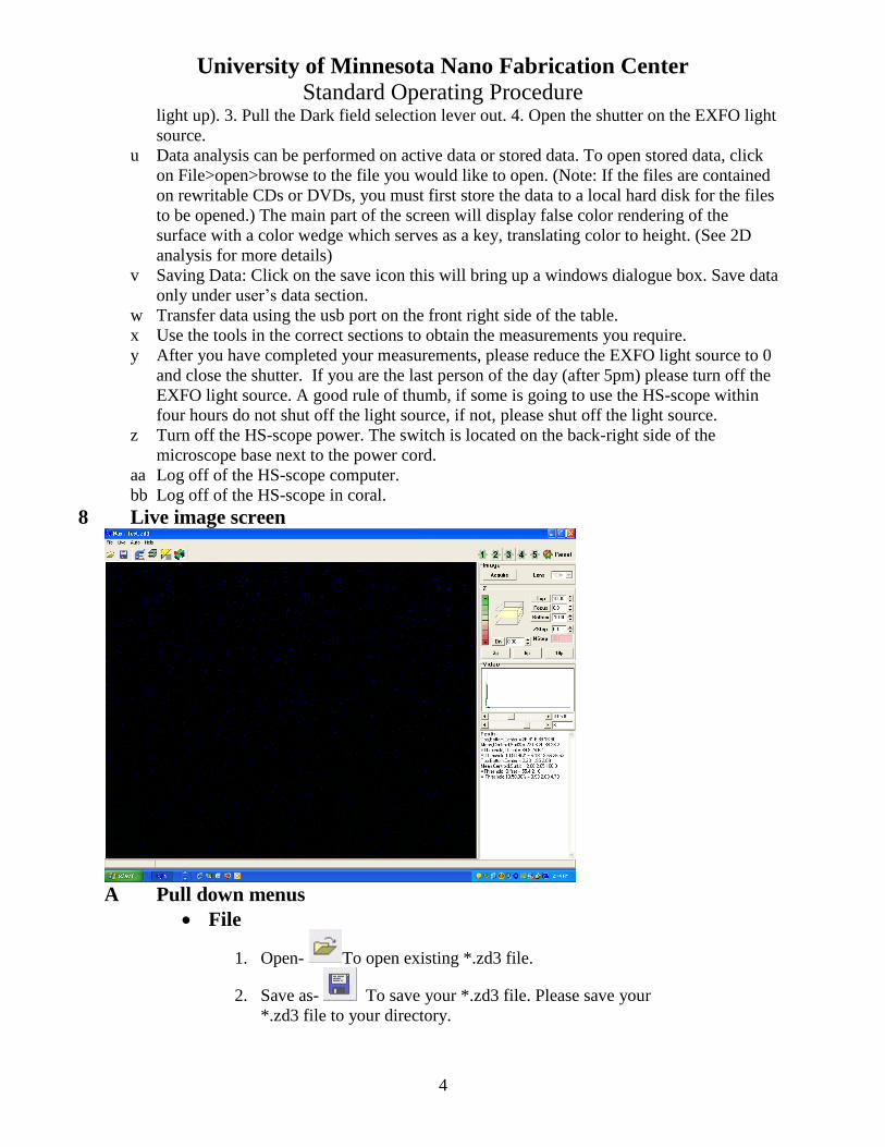
8 Live image screen
A Pull down menus
File
1. Open- To open existing *.zd3 file.
2. Save as- To save your *.zd3 file. Please save your
*.zd3 file to your directory.

University of Minnesota Nano Fabrication Center
Standard Operating Procedure
5
3. Show debug window-Shows debug window lower right hand corner.
4. Open surface*.BMP : Opens surface *.BMP.
5. Open intensity *.BMP: Not functional.
6. Save surface *.BMP: Saves surface *.BMP.
7. Save intensity *.BMP : Saves intensity *.BMP
Live 1. Camera Live: Toggles live camera on/off.
2. Show Debug: Not functional.
3. Bin 1 (1280x1024): Standard setting. Resolution of live image (1280 x
1024).
4. Bin 2 (640x512): Resolution of live image (640 x 512), smaller data file.
5. Bin 3 (320x256): Resolution of live image (320 x 256), smallest data file.
6. Clear volume
Auto 1. Auto Level: Toggles automatic leveling on/off.
2. Auto Reference: Toggles automatic reference on/off.
3. Auto Interpolation: Toggles automatic interpolation on/off.
4. Keep Tools: Saves tool set to a file.
Help 1. About: Hyphenated Systems.
B Icon below pull down menus.
1. Open File
2. Save as
3. Live image
4. Display slices- The displays the images taken.
5. 2D Processing
6. 3D Display
9 2D Processing screen

University of Minnesota Nano Fabrication Center
Standard Operating Procedure
6
A Pull down menus
File 1. Open-To open existing *.zd3 file.
2. Save as- To save your *.zd3 file. Please save your
*.zd3 file to your directory.
3. Show debug window-
4. Open surface*.BMP
5. Open intensity *.BMP
6. Save surface *.BMP
7. Save intensity *.BMP
View 1. Properties: Toggles right hand properties panel on/off.
2. Tool Selection: Toggles right hand tool selection panel on/off.
3. Display-Toggles right hand display panel on/off.
4. Readout: Toggles right hand readout panel on/off.
5. Roughness: Toggles right hand roughness panel on/off.
6. Threshold: Toggles right hand threshold panel on/off.
7. Zoom: Toggles right hand zoom panel on/off.
8. Calculation: Toggles right calculation panel on/off.
9. Default: Toggles on default panel settings.
10. Show Invalid Data: Dark green/ black/ interpolated
11. Do interpolation- Does interpolation on data set.
2D Tools
1. Points: Points mode Icon
Click on the “Points Mode” icon to evaluate the quality of the scan data. This
will bring up a graph of gray scale intensity of the selected pixel on the
vertical axis, against scan position along the horizontal axis. Holding down

University of Minnesota Nano Fabrication Center
Standard Operating Procedure
7
the left mouse button as the cursor is moved over the surface, the
graph will be continuously updated with the contrast curve for the pixel
designated – also indicated by a cross displayed on the surface. Releasing
the mouse button will freeze the cross and the data for that pixel. The red
lines on the following graph represent the algorithm output of surface
position at that pixel in the z direction (vertical line) and the maximum gray
level at that surface (when it was exactly in focus).
2. Line: Line mode. Display height profile for current cross section.
Clicking on the Line Mode icon enables cross sectional analysis of the
data. Line properties: None: No averaging is performed. Circular
window: An unweighted average of a circular area defined by the line
width is used Circular Hann window: A center-weighted circular
average is used. Wide line: An unweighted lateral average is used across
the line width. Wide line Hann window: A center-weighted lateral
average is used
3. Line Roughness: Display line roughness parameters for current
cross section.
4. Area: Shows all measurement areas and allows creation of new
ones.
5. Level: Shows all leveling areas and allows creation of new ones.
6. Pattern recognition: Shows all pattern recognition tools and allows
creation of new ones.
7. All Tools: Show all area tools, pattern recognition tools and line
tools on the screen at one time. In this mode, all tools can be moved as a
unit, maintaining their relative positions.
8. Roughness options: Roughness and waviness parameters may be changed.
9. Do reference:
10. Do level:
11. Do interpolation:
12. Do manual level:
13. Measure: Record current measurements in the results text box.
14. Recalc Z: Recalculate surface with current algorithm settings.
15. Clear all tools: Deletes all tools.
Graph 1. Copy as text: Copies a data set a file. First, a line must be made in line
mode, then using copy as text, paste the data set into a notepad document,
save document in your folder.
2. Copy as graph: Function does not work.
3. Display: Display has two modes, image only and image and graph.

University of Minnesota Nano Fabrication Center
Standard Operating Procedure
8
4. Show wedge: Displays color wedges in the lower right hand corner of the
image window.
5. Show Axes: Displays X and Y axes on the image window.
Auto 1. Auto level: Enables automatic leveling.
2. Auto Reference: Subtracts stored reference data from acquired data.
3. Auto Interpolation: Enables automatic interpolation.
4. Keep Tools: When this function is enabled it will save your tool set with
the *.zd3 file.
Adjusting Surface Calculations (from Hyphenated Systems
manual) 1. By default, the surface calculation algorithm finds the surface that shows
the largest contrast response with height. For a single opaque, surface this
allows the surface to be accurately rendered. In the case of transparent
films, however, the surface of interest may not be the one with the largest
contrast response.
Consider, for instance the case of an isolated photoresist feature on silicon.
In the bare silicon region, there is a single contrast response:
In the region of the photoresist, however, there are two responses. Some
light is scattered from the surface of the photoresist and some from the
silicon surface:

University of Minnesota Nano Fabrication Center
Standard Operating Procedure
9
Since the silicon surface shows a greater response than the photoresist
surface, this signal is the one traced by the default algorithm. Of course,
the silicon seen through the photoresist appears to be at a higher level than
the bare silicon because of the refractive index of the photoresist:
The interface to be rendered may be controlled by adjusting the
parameters of the Surface Calculation. Here, for example we can click on
the tab icon at the lop left hand corner of the chard and drag out a cursor,
placing it between the two peaks. Now, selecting Above Cursor in the
"Surface" pull-down in the Surface Calculation box the detected surface
switches to the upper, photoresist, peak.

University of Minnesota Nano Fabrication Center
Standard Operating Procedure
10
Clicking the "Calculate" button re-calculates the entire surface with this
new algorithm setting.
University of Minnesota Nano Fabrication Center
Standard Operating Procedure
11
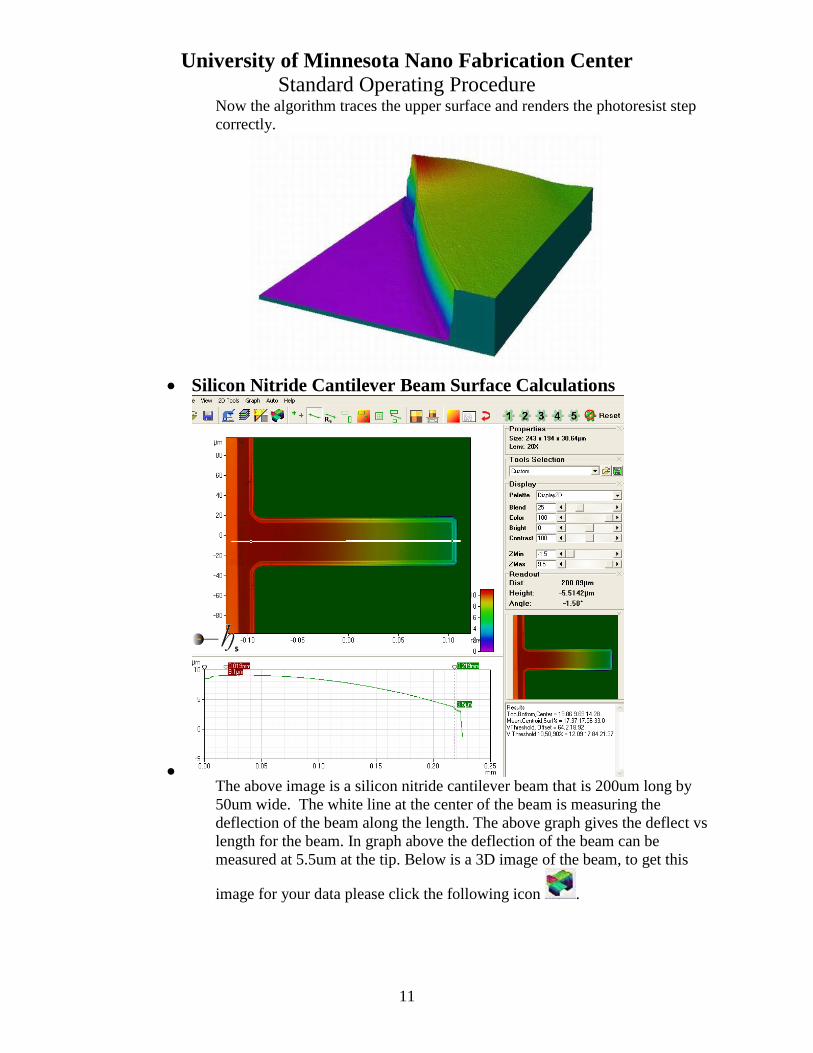
Now the algorithm traces the upper surface and renders the photoresist step
correctly.
Silicon Nitride Cantilever Beam Surface Calculations
The above image is a silicon nitride cantilever beam that is 200um long by
50um wide. The white line at the center of the beam is measuring the
deflection of the beam along the length. The above graph gives the deflect vs
length for the beam. In graph above the deflection of the beam can be
measured at 5.5um at the tip. Below is a 3D image of the beam, to get this
image for your data please click the following icon .

University of Minnesota Nano Fabrication Center
Standard Operating Procedure
12
To port this data to an excel file. To the following:
1. Graph>copy as Text.
2. Open excel and import your data.

University of Minnesota Nano Fabrication Center
Standard Operating Procedure
13
10 To make measurement on your sample. After you have acquired an image use points mode to check the signal strength.
Using line mode, draw a line from the left side to the right side of your screen. To
start the line left click and drag your mouse to the second location and double left
mouse button to end the line. If you would like to change the line properties
double click on the line mode icon in the tool bar. This will bring up a Line
Properties window in the lower right side of you screen. To change the wide of
the line see image below.

University of Minnesota Nano Fabrication Center
Standard Operating Procedure
14
Navigation image-Provides a means to zoom in on areas within the field-of-view
by clicking and dragging to create a zoom box. The main display is zoomed in
real time. Any tools present remain in their set positions with their set sizes. Zoom
box properties may be accessed by right-clicking the box. Changes to the tool size
and position made in the properties box and applied to the navigation image
transfer to the main display once the properties box is closed.
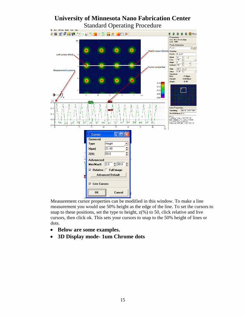
Measurement cursors- The location of the measurement cursor can be seen below. If you place the mouse
cursor over the measure cursor and right click, you will bring a window to define the
measurement cursors. See below.
University of Minnesota Nano Fabrication Center
Standard Operating Procedure
15
Measurement cursor properties can be modified in this window. To make a line
measurement you would use 50% height as the edge of the line. To set the cursors to
snap to these positions, set the type to height, z(%) to 50, click relative and live
cursors, then click ok. This sets your cursors to snap to the 50% height of lines or
dots.
Below are some examples.
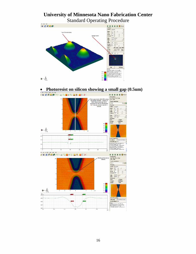
3D Display mode- 1um Chrome dots
University of Minnesota Nano Fabrication Center
Standard Operating Procedure
16
Photoresist on silicon showing a small gap (0.5um)

University of Minnesota Nano Fabrication Center
Standard Operating Procedure
17
Metal height measurement using area mode.
Metal height measurement using line mode.
Silicon etch
University of Minnesota Nano Fabrication Center
Standard Operating Procedure
18
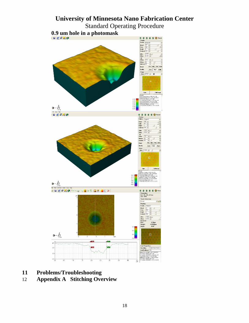
0.9 um hole in a photomask
11 Problems/Troubleshooting
12 Appendix A Stitching Overview


