
Upscaling of Lacustrine Groundwater Discharge by Fiber Optic
Distributed Temperature Sensing and Thermal Infrared imaging
Dissertation
zur Erlangung des akademischen Grades
doctor rerum naturalium
(Dr. rer. nat.)
im Fach Geographie
eingereicht an der
Mathematisch-Naturwissenschaftlichen Fakultät
der Humboldt-Universität zu Berlin
von
Agrarwirtchafts Ingenieurin Amaya Irene, Marruedo Arricibita
Präsidentin/Präsident der Humboldt-Universität zu Berlin
Prof. Dr.-Ing. Dr. Sabine Kurst
Dekanin/Dekan der Mathematisch-Naturwissenschaftlichen Fakultät
Prof. Dr. Elmar Kulke
______________________________________________________________________
Gutachter/innen:
1. Prof. Dr. Gunnar Nützmann
2. Prof. Dr. Jörg Lewandowski
3. Prof. Dr. Jan Fleckenstein
Tag der Einreichung: 4.12.2017
Tag der mündlichen Prüfung: 17.05.2018

i
Abstract
Groundwater (GW) and surface water (SW) are nowadays considered closely coupled entities
of a hydrological continuum. GW exfiltration into lakes (lacustrine groundwater discharge,
LGD) can have significant impacts on lake water quantity and quality. This entails the need to
understand the mechanisms relevant in the context of LGD and to develop and improve
measurement methods for LGD. Multiple approaches to identify and quantify LGD are based
on significant temperature differences between GW and lake water and the measurement of
related heat transport. The main aim of the present PhD thesis is to study signal propagation
from the point scale of LGD at the sediment-water interface across the overlying water body
to the water surface-atmosphere interface. The PhD thesis tests the hypothesis that the
positive buoyancy of warm GW causes upwelling across the cold water column and allows
the detection of LGD at the water surface by thermal infrared imaging (TIR). For that
purpose, a general conceptual framework is developed based on hierarchical patch dynamics
(HPD). It aims to guide the researchers in this field, on adequately combining multiple heat
tracing techniques to identify and quantify heat and water exchange over several spatial scales
and across ecohydrological interfaces in freshwater environments (Chapter 2). The conceptual
framework was used for the design of a mesocosm experiment (Chapters 3 and 4). Different
LGD rates were simulated by injecting relatively warm water at the bottom of an outdoor
mesocosm. A fiber optic distributed temperature sensing (FO-DTS) cable was installed in a
3D setup at multiple depths in the water column to trace the heat signal of the simulated LGD
under different weather conditions and over entire diurnal cycles. Additionally, a TIR camera
was mounted 4 meters above the mesocosm to monitor water surface temperatures. TIR
images were validated using FO-DTS temperature data 2 cm below the water surface (Chapter
4). The positive buoyancy of relatively warm LGD allows the detection of GW across the
water column and at the water surface-atmosphere interface by FO-DTS and TIR.
Hydrometeorological factors such as cloud cover and diurnal cycle of net radiation strongly
control: 1) the upwelling of simulated LGD across the water column (Chapter 3) and 2) the
reliability of TIR for detection of LGD at the water surface-atmosphere interface (Chapter 4).
In both cases, optimal results are obtained under overcast conditions and during night. Thus,
detection of upwelling of LGD across the water column and at the water surface-atmosphere
interface is only possible if heat fluxes related to LGD are not overshadowed by heat fluxes of
other sources across the water surface-atmosphere interface. Even though the present study
proves that the LGD signal can be identified by TIR at the water surface, it can also be
concluded that TIR will be only restrictedly applicable in real world case studies.
Keywords: Lacustrine groundwater discharge, Thermal infrared, Fiber optic distributed
temperature sensing, Heat tracing.

ii

iii
Zusammenfassung
Grund- und Oberflächenwasser werden heutzutage als hydraulisch eng verbundene
Kompartimente eines hydrologischen Kontinuums angesehen. Der Zustrom von Grundwasser
zu Seen (engl. lacustrine groundwater discharge, LGD) kann signifikante Auswirkungen auf
Qualität und Quantität des Seewasser haben. Dementsprechend besteht die Notwendigkeit die
zugrunde liegenden Prozesse zu verstehen und geeignete Methoden zur Erfassung von LGD
zu entwickeln. Viele Ansätze zur Identifikation und Quantifizierung von LGD basieren auf
signifikanten Temperaturunterschieden zwischen Grund- und Seewasser und der Messung des
damit einhergehenden Wärmetransports. Hauptziel der vorliegenden Doktorarbeit ist es,
Signalfortpflanzung und -ausbreitung des Grundwasserzustroms zu untersuchen – von der
Punktskala des LGD an der Sediment-Wasser Grenzfläche durch den Wasserkörper zur
Grenzfläche Wasseroberfläche-Atmosphäre. Die Doktorarbeit testet die Hypothese, dass das
im Verhältnis zum Umgebungswasser leichtere warme Grundwasser in der kalten
Wassersäule aufsteigt (engl. upwelling) und eine Detektion von LGD an der
Wasseroberfläche mit thermalen Infrarot (TIR) Aufnahmen erlaubt. Zu diesem Zweck wird
zunächst mit der „hierarchical patch dynamics (HPD)“ ein konzeptioneller Rahmen
entwickelt, der dazu dienen soll, eine angemessene Kombination multipler Techniken zur
Erfassung von Wärme- und Wasserflüssen anzubieten (Kapitel 2). Dabei sollen verschiedene
räumliche Skalen und ökohydrologische Grenzflächen in Süßwassersystemen abgedeckt
werden. Die HPD wurde als Grundlage für das Design eines Mesokosmos-Experimentes
genutzt (Kapitel 3 und 4). Dabei wurden unterschiedliche LGD-Raten durch den Zustrom von
relativ warmem Wasser am Grund eines Outdoor-Pools simuliert. Ein Glasfaserkabel (engl.
fibre-optic distributed temperature sensing, FO-DTS) wurde in einem 3D Aufbau in
verschiedenen Tiefen der Wassersäule installiert, um das Wärmesignal des simulierten
Grundwasserzustroms zu verfolgen – unter verschiedenen Witterungsbedingungen und im
Laufe eines kompletten Tagesgangs. Zusätzlich wurde 4 m über dem Mesokosmos eine TIR-
Kamera installiert, um die Temperatur des Oberflächenwassers aufzuzeichnen. Die TIR-
Aufnahmen wurden mit Temperaturen, die mit FO-DTS 2 cm unter der Wasseroberfläche
gemessen worden waren, validiert (Kapitel 4). Die Anwendung von FO-DTS und TIR
ermöglicht die Detektion von LGD in der Wassersäule und an der Grenzfläche
Wasseroberfläche-Atmosphäre. Hydrometeorologische Faktoren wie Wolkenbedeckung und
der Tagesgang der Netto-Strahlung kontrollieren: 1) den Auftrieb des simulierten LGD in der
Wassersäule (Kapitel 3) und 2) die Zuverlässigkeit von TIR bei der Erfassung von LGD an
der Grenzfläche zwischen Wasseroberfläche und Atmosphäre (Kapitel 4). In beide Fällen
werden die besten Ergebnisse bei Wolkenbedeckung und nachts erzielt. Das heißt, dass der
Auftrieb von LGD in der Wassersäule und an der Grenzfläche zwischen Wasseroberfläche
und Atmosphäre nur erfasst werden kann, wenn die LGD-bedingten Wärmeflüsse nicht durch
andere Wärmeflüsse über die Grenzfläche zwischen Wasseroberfläche und Atmosphäre
überdeckt werden. Obwohl die vorliegende Studie zeigt, dass das LGD-Signal mit TIR an der
Wasseroberfläche erfasst werden kann, muss einschränkend auch der Schluss gezogen
werden, dass TIR unter realen in-situ Verhältnissen nur bedingt anwendbar sein wird.
Schlagwörter: Lacustrine groundwater discharge, Thermalen Infrarot, Fiber optic distributed
temperature sensing, Wärme als Tracer

iv
v
Table of contents
1 Introduction ......................................................................................................................... 1
1.1 Motivation to study groundwater-surface water interactions ........................................ 1
1.2 State of the Art: GW-SW interactions ........................................................................... 3
1.2.1 Mechanisms of GW-SW interactions ..................................................................... 3
1.2.2 Factors controlling GW-SW interactions .............................................................. 4
1.2.3 GW discharge in lakes ........................................................................................... 5
1.2.4 GW discharge in streams....................................................................................... 6
1.3 Measurement methods for GW-SW interactions........................................................... 6
1.4 Heat as a natural tracer of GW-SW interactions ........................................................... 8
1.4.1 Heat tracing in stream and lake beds .................................................................... 9
1.4.2 Heat tracing in the water column ........................................................................ 11
1.5 Scaling in hydrology ................................................................................................... 13
1.5.1 Can we learn from other disciplines? ................................................................. 16
1.6 Hypothesis and aims of this PhD thesis ...................................................................... 17
1.7 References ................................................................................................................... 18
2 Scaling on temperature tracers for water and heat exchange processes in ecohydrological
interfaces .................................................................................................................................... 28
2.1 Introduction ................................................................................................................. 30
2.2 Theory and methodology of hierarchical patch dynamics ........................................... 32
2.2.1 Hierarchy theory ................................................................................................. 33
2.2.2 Patch dynamics in landscape ecology ................................................................. 34
2.2.3 Hierarchical patch dynamics .............................................................................. 35
2.3 Application of HPD to water and heat fluxes in freshwater environments ................. 36
2.3.1 Structure of the HPD scheme for generic freshwater environments ................... 36
2.4 Heat tracing techniques in ecohydrological interfaces ................................................ 39
2.5 Proof of concept: vertical upscaling of discrete GW upwelling by FO-DTS and TIR 43
2.6 Synthesis, conclusions and recommendations ............................................................. 46
Acknowledgments ................................................................................................................... 48
Supplementary information ..................................................................................................... 48
References ............................................................................................................................... 49
Annex S1: Definitions ............................................................................................................. 55
3 Mesocosm experiments identifying hotspots of groundwater upwelling in a water column by
fiber optic distributed temperature sensing ............................................................................ 58
3.1 Introduction ................................................................................................................. 60
3.2 Material and methods .................................................................................................. 62
3.2.1 Experimental setup .............................................................................................. 62
vi
3.2.2 Data analyses and spatial statistics .................................................................... 65
3.2.3 Preprocessing and sources of error .................................................................... 66
3.2.4 Quantification of net heat fluxes across the water surface, advective heat fluxes and
internal energy change ........................................................................................................ 67
3.3 Results ......................................................................................................................... 67
3.3.1 FO-DTS observed temperature patterns ............................................................. 67
3.3.2 Quantitative analysis of spatial temperature patterns ........................................ 70
3.3.3 Net heat fluxes across the water surface, advective heat fluxes and internal energy
change ............................................................................................................................. 76
3.4 Discussion ................................................................................................................... 80
3.5 Conclusion ................................................................................................................... 87
Acknowledgments ................................................................................................................... 87
Supporting information ........................................................................................................... 87
References ............................................................................................................................... 89
Appendix S1: Quantification of interfacial heat transfer and net-advective heat flux ............ 94
Appendix S2 Nomenclature .................................................................................................... 97
4 Thermal infrared imaging for detection of groundwater at the surface of stagnant
freshwater bodies ..................................................................................................................... 102
4.1 Introduction ............................................................................................................... 104
4.2 Methods ..................................................................................................................... 106
4.2.1 Experimental design .......................................................................................... 106
4.2.2 Measurement protocol and calibration ............................................................. 108
4.2.3 Study period and influence of discharge rates, weather conditions and diurnal cycle
........................................................................................................................... 109
4.2.4 Comparison of TIR temperature data with FO-DTS temperature data ............ 110
4.3 Results ....................................................................................................................... 111
4.3.1 Comparison of TIR temperature data with FO-DTS temperature data ............ 111
4.4 Discussion ................................................................................................................. 116
4.4.1 Comparison of TIR temperature data with FO-DTS temperature data ............ 116
4.4.2 Influence of discharge rates, weather conditions and the diurnal cycle ........... 116
4.4.3 Experimental shortcomings and future improvements ...................................... 118
4.4.4 Implications of results for TIR based monitoring of groundwater upwelling .......... 119
4.5 Conclusions ............................................................................................................... 120
Acknowledgments and Data .................................................................................................. 121
References ............................................................................................................................. 122
5 Synopsis ............................................................................................................................ 130
5.1 Summary of results .................................................................................................... 130

vii
5.2 Discussion ................................................................................................................. 130
5.2.1 Impacts of diurnal cycle of net radiation and cloud cover on tracing of LGD . 130
5.2.2 FO-DTS for monitoring LGD in lakes ............................................................... 132
5.2.3 TIR imaging for detection of LGD at the lake surface ...................................... 133
5.2.4 Combination of multiple heat tracing techniques for scaling of GW-SW interactions
across ecohydrological interfaces ..................................................................................... 134
5.3 Conclusions ............................................................................................................... 136
5.4 Future direction ......................................................................................................... 137
5.5 References ................................................................................................................. 139
Acknowledgements .................................................................................................................. 144
Declaration of independent work ........................................................................................... 145

viii
List of figures Figure 1.1 Unsaturated zone, saturated zone, GW and SW in freshwater systems (Taken and modified
from Winter, 1998). ....................................................................................................................... 4
Figure 1.2 Sediment temperatures against depth (z): for gaining and losing conditions (green and red
lines respectively) and for daily (in italic) or annual cycles. For annual cycles the depth at which the
temperature reaches a constant value can be 10 m or more at downward flow. On the contrary, the
depth at which the temperatures reach constant values at upward flows can be less than 1 meter. Taken
from Constantz and Stonestrom (2003). ...................................................................................... 11
Figure 2.1 Conceptualization of heat and water exchange processes at freshwater ecosystem across
several ecohydrological interfaces. ............................................................................................. 31
Figure 2.2 Hierarchical conceptualización of heat and water exchange processes at freshwater
ecosystems at different spatial and temporal scales and across different ecohydrological interfaces.
..................................................................................................................................................... 34
Figure 2.3 An HPD based conceptual guideline on how to adequately observe water/heat exchange
processes across spatial scales and ecohydrogological interfaces by combination of different heat
tracing techniques. ....................................................................................................................... 38
Figure 2.4 Application of different experimental temperature tracing techniques to identify heat and
water fluxes at different ecohydrological interfaces in freshwater environments defined in Figures 2.1,
2.2 and 2.3. .................................................................................................................................. 42
Figure 2.5 Example for vertical scaling of water and heat exchanges related to simulated LGD.44
Figure 3.1 Sketch of the experimental set up showing a cross section through the mesocosm including
the fibre optic distributed temperature sensing set up. ................................................................ 63
Figure 3.2 (a) Raw temperature data (black line) and smoothed temperature data with local
polynomial regression fitting (LOESS; red line) and (b) temperature difference between raw
temperature data and smoothed temperature data. ...................................................................... 67
Figure 3.3 Slice3D plots visualizing for the four layers of DTS measurements the difference from the
minimum temperature of each dataset. Values averaged for approximately 12 hr day (always left of
colour scale) or night (always right), respectively. Different injection rates and weather conditions as
follows: (a) 1 L min−1 clear 19.03.2015, (b) 1 L min−1 partly cloudy 25.03.2015, (c) 5.5 L min−1 clear
18.03.2015, (d) 1 L min−1 overcast 26.03.2015, (e) 5 L min−1 overcast 27.03.2015, and (f) 15 L min−1
overcast 12.03.2015. inlet of cold lake water, inlet of warm water, outlet of mixed water from
mesocosm. clear day, clear night, partly cloudy day, partly cloudy night,
overcast day, and overcast night. ......................................................................................... 69
Figure 3.4 (a) and (b) Moran's I scatterplots, (c) and (d) LISA maps, (a) and (c) for 1 L min−1 clear
sky, day, (b) and (d) for 15 L min−1 overcast sky, day. In (a) and (b), potential influencing measures
for the linear relationship between the data and the lag are highlighted as red diamond shape. In (c)
ix
and (d), red coloured points belong to the high-high quadrant in Moran's I scatterplot, yellow coloured
points belong to the low-low quadrant in Moran's I scatterplot, and blue coloured points are spatially
nonsignificant points. From top row to bottom row: Layers 4, 3, 2, and 1. ................................ 71
Figure 3.5 Moran's I values. (a) Day, clear and partly cloudy sky; (b) night, clear and partly cloudy
sky; (c) day, overcast sky; and (d) night, overcast sky. All plots are plotted from lowest to highest
injection rates. ............................................................................................................................. 72
Figure 3.6 Spatial correlation coefficients for (a) day, clear sky and partly cloudy conditions; (b) night
and clear sky, partly cloudy conditions; (c) day and overcast conditions; (d) night and overcast
conditions. ................................................................................................................................... 75
Figure 3.7 Calculated heat fluxes across the water surface (G), net radiation (Rn) evaporative heat flux
(λE), and sensible heat flux (H) for (a) control dataset with 0 L min−1
injection rate, overcast, (c) 1 L
min−1
clear, (e) 1 L min−1
partly cloudy, (g) 1 L min−1
overcast, (i) 5.5 L min−1
clear, (k) 5 L min−1
overcast, and (m) 15 L min−1
overcast and calculated ΔE, EG and Eadv for (b) control experiment
overcast (d) 1 L min−1
clear, (f) 1 L min−1
partly cloudy, (h) 1 L min−1
overcast, (j) 5.5 L min−1
clear,
(l) 5 L min−1
overcast, and (n) 15 L min−1
overcast. ................................................................... 78
Figure 3.8 Change of energy (ΔE) over time for seven datasets: 1 L min−1
clear, 1 L min−1
partly
cloudy, 1 L min−1
overcast, 5.5 L min−1
clear, 5 L min−1
overcast, 15 L min−1
overcast, and control
dataset with 0 L min−1
injection rate, overcast conditions. .......................................................... 79
Figure 3.9 Conceptual model of spatial distribution of injected water in the water column under
different weather conditions, for different injection rates during (a) day and (b) night. (a.1) and (b.1) 1
L min−1
, clear sky; (a.2) and (b.2) 1 L min−1
, partly cloudy sky; (a.3) and (b.3) 1 L min−1
, overcast sky;
(a.4) and (b.4) clear sky, 5.5 L min−1
; (a.5) and (b.5) 5 L min−1
, overcast sky; (a.6) and (b.6) 15 L
min−1
, overcast sky. The degree of the signal strength is indicated by the intensity of the red colour:
Light red: weak signal, dark red: strong signal. The size of the arrows indicates the strength of the Rnl
and Rns. The blue colour indicates the losses of energy from the mesocosm. The red colour indicates
the gains of energy in the mesocosm. .......................................................................................... 83
Figure 4.1 Schematic of the mescocosm experimental design including TIR setup and the upper layer
of the FO-DTS. .......................................................................................................................... 107
Figure 4.2 Visual comparison of TIR temperature data with FO-DTS temperature data. Worst (left)
and best (right) spatially correlated datasets for overcast conditions at three injection rates: a) 1 L
min−1
, b) 5 L min−1
and c) 15 L min−1
. Temperature signal corresponding to the warm water injection
is indicated with a black arrow in Fig. 4.2a and b. .................................................................... 113
Figure 4.3 Visual comparison of TIR temperature data with FO-DTS temperature data. Worst (left)
and best (right) correlated datasets for clear conditions at three injection rates: a) 1 L min−1
and b) 5 L
min−1
. ......................................................................................................................................... 114
x
Figure 4.4 Bivariate Global Moran’s I values for spatial correlation between FO-DTS and TIR
temperature data under overcast weather conditions, for three injection rates: a) 1 L min−1
, b) 5 L
min−1
and c) 15 L min−1
. ............................................................................................................ 115
Figure 4.5 Bivariate Global Moran’s I values for spatial correlation between FO-DTS and TIR
temperature data under clear sky conditions, for two injection rates: a) 1 L min−1
and b) 5 L min−1
.
................................................................................................................................................... 115
List of tables Table 1.1 LGD examples reported as percentage of the lake water balance and as absolute rates.
....................................................................................................................................................... 3
Table 2.1 Summary of the heat tracing techniques that are considered in this paper for scaling of water
and heat fluxes in freshwater environments: scales, limitations and recommendations. Scales used in
this paper are: Point/Small (few cm), local (cm to few m), reach, plot or lake shore (from few m),
stream, land or lake (from m to km) and finally catchment (from km). “Temp.” goes for temperature.
..................................................................................................................................................... 41
Table 4.1 24-hour measurements with FO-DTS and TIR camera. The control dataset is only used as a
reference for the initial conditions of the mesocosm measurements and is not included in the results.
................................................................................................................................................... 109
Table S1 Spatial correlation coefficients between layers. ........................................................ 100
List of abbreviations GW: Groundwater
SW: Surface water
LGD: Lacustrine groundwater discharge
HZ: Hyporheic zone
HEF: Hyporheic exchange flow
FO-DTS: Fiber optic distributed temperature sensor
TIR: Thermal infrared
HPS: Heat pulse sensor
HT: Hierarchy theory
PD: Patch dynamics
HPD: Hierarchical patch dynamics

Introduction
1
1 Introduction
1.1 Motivation to study groundwater-surface water interactions
Freshwater is essential for human life and societies. Lakes, rivers and aquifers, among others,
are important sources of freshwater. Therefore preserving quality and quantity of freshwater
in these systems is crucial. In addition, it is important to maintain the integrity of these
freshwater systems because they provide multiple services such as flood control, habitats for
numerous plant, animal and other species, production of fish or purification of human and
industrial wastes. The failure to keep the integrity of theses freshwater systems will lead to
loss of species and other of the above mentioned ecosystems services (Baron et al., 2002). In
2015, the European Environmental Agency (EEA) reported that more than half of the rivers
and lakes in Europe did not hold a good ecological status as requested by the European Water
Framework Directive (EC, 2000) (European Environmetal Agency, 2015). Furthermore, about
25% of groundwater across Europe had a poor chemical status in 2015 according to the EEA.
At European level, groundwater is the most important drinking water source in many
European regions (Bartel et al., 2016). Nowadays´ widespread intense agriculture is often
claimed to be responsible for the situation described above. Agricultural activities often
include intensive use of pesticides and fertilizers that end up in surface waters (SW) and
groundwater (GW). In addition, discharge of waste water from industry, transport, mining and
households are also a source of pollution for freshwaters (European Environmetal Agency,
2015). GW and SW are often hydrologically closely connected and by that might influence
each other in quality and quantity (Winter et al., 1998). Therefore, knowledge on how GW is
connected to SW can be of major relevance to design successful management strategies
(Winter et al., 1998) to maintain or improve the quality and quantity of GW and SW.
For a long time, GW and SW have been studied as individual entities. In fact, GW and SW
differ to some extent in their chemical, biological and physical features (Kalbus et al., 2006).
However, over the last decades, an important paradigm shift has taken place: from a static
image of rivers, lakes and aquifers as discrete bodies, respectively, to a more complex and
dynamic interpretation of GW and SW as undivided constituents of a stream/lake-catchment
continuum (Krause et al., 2011). Thus, GW and SW are now considered as connected entities
(Winter et al., 1998) which interact across and within different interfaces. The interfaces
where GW and SW interact are generally distinguished by permeable sediments with
saturated conditions and low flow velocities (e.g. the hyporheic zone (HZ) in streams or
2
lacustrine sediments in lakes) (Kalbus et al., 2006). Dynamic and non-stationary
biogeochemical and physical processes take place at these interfaces (Krause et al., 2017),
which include transport, degradation, transformation, precipitation or sorption of compounds
(Kalbus et al., 2006). These interfaces can contribute significantly to SW metabolism and
biota as well (Brunke and Gonser, 1997). Thus, GW-SW interactions have a relevant
influence on the water quality of SW bodies such as streams and lakes as well as on aquifers
(Kalbus et al., 2006).
In the last decades, there has been an increased interest in GW-SW interactions (Fleckenstein
et al., 2010). With the adoption of The European Water Framework Directive (EC, 2000) in
2000 the motivation to investigate GW-SW interactions increased even more. The relevance
of GW-SW interfaces has been acknowledged by several authors who described GW-SW
interfaces as “hotspots” (areas of intensified activity: Frei et al., 2012; Krause et al., 2013) or
areas, where interaction between GW and SW takes place (Winter, 1999; Krause et al., 2011;
Lewandowski et al., 2014). Nevertheless, complete understanding on the functioning of these
“hotspots” is still a knowledge gap necessary to describe GW-SW interactions in aquatic
environments.
In lakes, all flow of GW from the lake bed (i.e. the interface) to the lake is referred to as
lacustrine groundwater discharge (LGD) (Lewandowski et al., 2014). GW-SW interactions in
lake systems might be different to the ones observed at stream-aquifer interfaces (i.e. in the
HZ). Therefore, different definitions and influencing factors come into consideration.
Research on GW-lake interactions is not as common as research on GW-streams interactions
and the function of the HZ (Lewandowski et al., 2014). Especially when it comes to water and
nutrient budgets LGD has long been ignored due to several reasons, (Meinikmann et al.,
2013; Lewandowski et al., 2014):
Difficulty of access the interface due to the depth of lakes
Low local discharge rates due to large extent of the interface
Lack of appropriate methodology
Large spatial and temporal variability of discharge rates and GW composition which
requires high numbers of measurements in order to get reliable estimates of the LGD
component in budgets
GW can be relevant in nutrient budgets even if it is not relevant in water budgets
because concentrations in groundwater might be much higher than in lake water.

Introduction
3
For example, Meinikmann et al. (2015) demonstrated that more than 50% of external
phosphorus loads to an eutrophied lake, were discharged by GW. By that LGD was identified
to be a main driver of lake eutrophication. In this example LGD accounted for only about
25% of the lake´s water balance. In contrast to that, LGD is often the dominant component in
the water balance of lakes (Table 1, Lewandowski et al., 2014). By that they have the natural
potential to also contribute significantly to the quality of these lakes.
Table 1.1 LGD examples reported as percentage of the lake water balance and as absolute rates.
LGD as percentage of the lake water
balance (%)
LGD rates
LGD represents 74% of all inflows to
Williams Lake, Minnesota (Labaugh et al.,
1997).
477 L m-2
d-1
for Ashumet Pond,
Massachusetts (McCobb et al., 2009)
LGD represents 94% to Mary Lake,
Minnesota (Stets et al., 2010).
155 L m-2
d-1
for Dickson Lake, Ontario
(Ridgway and Blanchfield, 1998)
LGD represents 90% to Cliff Lake,
Montanna (Gurrieri and Furniss, 2004).
138 L m-2
d-1
Shingobee Lake, Minnesota
(Rosenberry et al., 2000)
LGD represents 85% to Lake Annie, Florida
(Sacks et al., 1998)
Although the main focus of the present PhD thesis is on LGD, GW discharge to streams is
also considered in some chapters to compare it with LGD and to transfer knowledge from
GW-SW interfaces in streams to GW-SW interfaces in lakes.
1.2 State of the Art: GW-SW interactions
1.2.1 Mechanisms of GW-SW interactions
In the unsaturated zone the soil pores are filled with air and water and in the saturated zone
the soil pores are only filled with water. Water in the unsaturated zone usually percolates
downwards to the saturated zone. Subsurface water in the saturated zone moves generally in
the direction of the steepest hydraulic gradient. The upper part of the unsaturated zone is
called soil-water zone. Water in that zone might be used by plants or evaporate to the
atmosphere. The water in the saturated zone is called GW and the upper boundary of this zone
is called water table. When the GW is connected to SW bodies the water table touches SW
bodies at the shore or near the shore line (see Figure 1.1) (Winter et al., 1998).

4
Figure 1.1 Unsaturated zone, saturated zone, GW and SW in freshwater systems (Taken and modified
from Winter, 1998).
Flow across the GW-SW interface occurs in two directions. On the one hand, water can flow
from the aquifer through the stream or lake bed into the stream or lake, respectively. This
process is called exfiltration – a term which we define from the perspective of the aquifer
(please note that other authors use a different definition and call the process which we call
exfiltration, infiltration). Such streams are called gaining streams and in lakes the process is
termed LGD. GW inflow into the stream or lake can occur at diffuse or at discrete localized
inflow points (Winter, 1998; Lewandowski et al., 2014). On the other hand, water can flow
through the streambed or lake bed into the aquifer, this process is called infiltration and the
system is called loosing stream or loosing lake, respectively (Winter et al., 1998; Constantz
and Stonestrom, 2003).
When GW discharges into SW (e.g. in streams or lakes) the chemical composition of the SW
will be impacted by the differing chemical composition of the GW. In addition, when GW
flows across the stream or lake bed various chemical reactions can take place that result in a
change of the composition of the exfiltrating GW. When water infiltrates into the stream or
lake bed the chemical composition of the SW will also impact the subsurface water in the HZ
or lacustrine sediments (Constantz and Stonestrom, 2003).
1.2.2 Factors controlling GW-SW interactions
GW-SW interactions are mainly controlled by:
Hydraulic head gradients between aquifer and stream/lake (Constantz and Stonestrom,
2003).
Spatial distribution and variability of hydraulic conductivity of sediments in the HZ or
lacustrine sediments and the underlying aquifer (Brunke and Gonser, 1997; Genereux
et al., 2008; Leek et al., 2009; Angermann et al., 2012a; Blume et al., 2013).

Introduction
5
In an unconfined aquifer the hydraulic head equals the water level. In a confined aquifer the
hydraulic head equals the pressure. Subsurface water flows from higher to lower heads. At the
stream or lake surface, the water pressure is zero as well as at all points on the water table (in
unconfined aquifer conditions). In this manner, the elevation of the water table regarding the
stream or lake surface will indicate the direction of the subsurface water flow between the
stream/lake and the near-shore aquifer. For instance, if the stream or lake is gaining, that
means that the elevation of the GW table is higher than the SW level. On the contrary, in
losing stream reaches or sections of the lake, the elevation of the GW table will be lower than
the stream or lake water level (Kalbus et al., 2006). Both kinds of interaction might occur
simultaneously in different parts of the stream or lake (Winter et al., 1998).
Some other variables impacting on exchange flows are:
Pressure changes due to the presence of geomorphological characteristics in the river
bed: pool riffle series, changes in slope, ripples or woody debris (Elliott and Brooks,
1997; Tonina and Buffington, 2007; Cardenas, 2009) or pressure changes due to wave
action and currents in lakes (Rosenberry et al., 2013).
The redistribution of sediments on the stream bed or lake bed also might play an
important role regarding seepage rates. Sometimes, the sediments can clog the stream
or lake bed leading to lower infiltration rates through the HZ or lacustrine sediments.
They can also trap stream or lake water between their interstices and enhance
interstitial water release into the stream or lake (Elliott and Brooks, 1997; Rosenberry
et al., 2010). Finally, due to wave action (e.g. during storm events), fine sediments in
the shore of the lakes can be resuspended and settle again in deeper regions of the lake
affecting seepage rates at the shore of the lake (Rosenberry et al., 2015).
Turbulence in the flowing stream water might induce upwelling and downwelling.
Geological heterogeneities within the alluvial aquifer and GW discharge area.
(Cardenas and Wilson, 2006; Fleckenstein et al., 2006; Frei et al., 2009; Engdahl et
al., 2010) or local geological conditions (Winter, 1999).
Stream or lake position relative to GW flow systems (Winter, 1999; Woessner, 2000).
1.2.3 GW discharge in lakes
In lakes GW discharge rates are often small, there is lower turbulent mixing in the lake water
than in the stream water and volume ratio between the water body in regards to the
discharging GW, is higher than in streams. Under homogeneous conditions with
homogeneous geology exchange flows are focused to near shore areas (Lewandowski et al.,

6
2014). The major reason is that flow lines approaching a lake bend upwards. An additional
reason for higher GW release in near shore areas is the spatial distribution of fine grained and
low permeability muddy material. The accumulation of muddy material is lower in areas close
to shore since wave action influences the distribution of sediments within the lake. Sediments
close to the shore will be easily resuspended and redistributed within the lake bed, while
sediments in deeper parts of the lake won’t be affected so intensively by wave action and
therefore less resuspended and redistributed (Rosenberry et al., 2015). This fact will lead to
higher hydraulic conductivities near shore than offshore (McBride and Pfannkuch, 1975;
Krabbenhoft et al., 1990; Kishel and Gerla, 2002). Some other times, if the aquifer has
hydraulically highly conductive areas, the GW will mainly flow through those areas following
preferential flow paths into the lake. Sometimes, if the lake is set on fractured rocks it will
show much localized LGD on the fractures of the rocks. Finally, lakes that are in contact with
more than one aquifer might show high GW discharge rates below the aquitard layer (low
permeability layer) separating both aquifers (Lewandowski et al., 2014).
1.2.4 GW discharge in streams
The HZ is defined conceptually as the saturated interstitial zones under the streambed and in
the stream bank that contains at least some parts of channel water (White et al., 1993).
Sometimes, low hydraulic conductivity streambed sediments inhibit GW upwelling and
enhance horizontal pore water movement in the HZ since GW upwelling is inhibited by
horizontal low-conductivity layers. Some other times, GW upwelling might be enhanced by
high hydraulic conductivity of streambed sediments near confining riverbed structures,
supplying a preferential flow path for rapid upwelling of semi-trapped GW (Angermann et al.,
2012a). The HZ in streams has been highlighted as an important ecohydrological interface
with intense biogeochemical processes. It is characterized by high spatial and temporal
heterogeneity in terms of sediment and discharge variability (Krause et al., 2011;
Lewandowski et al., 2011).
1.3 Measurement methods for GW-SW interactions
Many methods exist to measure GW-SW interactions. The methods can be applied in the
aquifer, in the SW, or in the HZ or lacustrine sediments. The methods vary in resolution,
sampled volume and time scale. Usually, the choice of a method requires balancing between
resolution, heterogeneities and sampled volumes. What is more, the scale of the method
chosen might have a relevant impact on the results. The impact of the scale on measurements
in heterogeneous media means that even if measurements are conducted with a dense grid of
Introduction
7
points, the results obtained might be different from those obtained at larger scales due to the
possibly large role of small-scale heterogeneities. For example, the role of small and high
conductivity areas might be underestimated with point measurements (Kalbus et al., 2006).
As another example, GW discharge in streams and hyporheic exchange flow (HEF) might not
be clearly distinguished when using the wrong scale. This is related to the high spatial
variability of flow patterns on small spatial scales in the HZ or in lacustrine sediments
(Schmidt et al., 2006; Lewandowski et al., 2011; Angermann et al., 2012). Additional
measurements are always advised to clearly determine the type of GW-SW interaction
occurring in the HZ or lacustrine sediments (Kalbus et al., 2006).
The research goal also has an important role when selecting the most appropriate methods to
describe GW-SW interactions (Kalbus et al., 2006) because it will determine the scale at
which techniques for measurements of GW-SW interactions are applied. For instance, for
regional studies large scale techniques are more appropriate. On the contrary, for process
studies high resolution measurements might be needed. Of course all methods have their own
limitations and uncertainties. For instance, at stream reach scales a high density measuring
network is needed which takes into account small scale patterns of flow (Schmidt et al.,
2006). Unfortunately that requires high device and measurement efforts. As a result, these
measurements are usually constrained to small spatial scales. For these reasons, there is a
requirement for inexpensive and quantitative methods which allow describing the spatial
heterogeneity of GW-SW interactions more adequately. Under ideal conditions, GW-SW
interactions should be characterized by a high amount of measurements (high temporal
resolution) with high spatial accuracy (Schmidt et al. 2006).
Several authors (Palmer et al., 1993; White et al., 1993; Kalbus et al., 2006; Schmidt et al.,
2006; Krause et al., 2011) have stated the need of multi-dimensional research methods which
could cope with several spatial and temporal scales in order to adequately describe GW-SW
interactions in aquatic ecosystems. A multi scale approach bringing together different
techniques can substantially decrease uncertainties and improve estimates of water fluxes
between GW-SW interfaces (Kalbus et al., 2006). For instance, Blume et al. (2013) combined
LGD rates derived from temperature lances or vertical hydraulic gradients (VHG) with 2-D
patterns of lake bed temperatures monitored by fiber optic distributed temperature sensing
(FO-DTS) for successful upscaling of LGD.
Therefore, the right selection of methods is of major importance for getting useful data
(Kalbus et al., 2006) to describe GW-SW interactions. For instance, GW-SW interactions can
be followed by monitoring the chemical composition of the water that is exchanged. The flow

8
path can be followed at different scales, from small to catchment scale (Constantz and
Stonestrom, 2003). Another method for tracing water flow is heat tracing. Natural variations
of temperature in areas close to the stream or lake environment are easy to track since
temperature can be easily measured during specific seasons and when exchange is fast
(Anderson, 2005).
In addition to the scale, the research goal and the selection of the most adequate method are
three key steps to characterize GW-SW interactions in freshwater bodies. Conant Jr (2004)
and Keery et al. (2007) advise the development of a conceptual model that considers the
main mechanisms that influence water flow across GW-SW interfaces.
Regarding the main focus of interest of the present PhD thesis, which is LGD, Lewandowski
et al. (2014) listed methods for LGD detection in three different groups:
Spatially specific methods which measure LGD rates in one point or over a small area,
for instance seepage meters (Lee, 1977), sediment temperature depth profiles (Schmidt
et al., 2006).
Integrating methods that quantify the entire GW inflow into a lake e. g. radon balances
(Kluge et al., 2007), stable isotope methods (Hofmann et al., 2008), annual GW
recharge in the subsurface catchment by modelling or computation of the water
budget.
Identification of discharge patterns without quantification of LGD such as fiber optic
distributed temperature sensing (FO-DTS) (Selker et al., 2006b), geophysical
approaches around the lake perimeter (Ong et al., 2010), airborne measurements of
thermal infrared radiation (TIR) (Lewandowski et al., 2013).
In the present PhD thesis, methods based on heat as a tracer to study GW-SW interaction in
stagnant waters (or LGD) will be the main focus of interest.
1.4 Heat as a natural tracer of GW-SW interactions
Natural heat tracing techniques allow monitoring the heat transported by groundwater or
surface water (Constantz and Stonestrom, 2003). The use of heat as a tracer for GW-SW
interactions, is based on the fact that GW temperatures are more or less stable throughout the
year whereas stream or lake temperatures change daily and seasonally (Kalbus et al., 2006).
Relevant differences between GW and SW temperatures can be observed during summer and
winter periods (Meinikmann et al., 2013) at the sediment profile of stream and lake beds and
at the water body.
Introduction
9
1.4.1 Heat tracing in stream and lake beds
Measurements of stream or lake bed temperatures can be used if there are large GW-SW
temperature differences. The results can be used to observe the propagation of the heat signal
through the sediment bed and to determine flow directions within the sediment (Anderson,
2005; Keery et al., 2007; Schmidt et al., 2007; Anibas et al., 2009; Hatch et al., 2010) to
determine GW discharge or recharge areas (Kalbus et al., 2006) or to compute exchange
fluxes (Westhoff et al., 2007; Hatch et al., 2010).
Stream/lake bed heat transfer is governed by three processes (Hannah et al., 2004; Constantz,
2008; Webb et al., 2008):
1. Advective or convective (free or forced) heat transfer
2. Conductive heat transfer
3. Radiative heat transfer
The horizontal and vertical distribution of heat in stream/lake beds is due to heat transport by
moving water (advective heat flow) and by heat or thermal conduction across the solid and
fluid phase of the sediments (conductive heat flow) (Constantz and Stonestrom, 2003;
Schmidt et al., 2007). The terms “advective heat transfer” and “convective heat transfer” are
used interchangeably in hydrology (Anderson, 2005). Sometimes convective heat transfer is
defined as heat transfer by moving water when water flows above the stream/lake bed in order
to differentiate advective and convective heat transfer processes (Constantz, 2008). In the
present PhD thesis, advective and convective heat transfer processes are considered
synonyms. To avoid confusion only one term is used. Free convection is understood as the
heat transfer by flow driven due to density differences in response to temperature differences
(e.g. in freshwater systems). Forced convection is heat transfer due to flow driven by other
mechanisms. For instance, forced convection is a common phenomenon in GW systems
where heat is transported by the movement of GW by recharge or discharge processes
(Anderson, 2005). Radiative heat transfer takes place when sun radiation is absorbed by the
water body or the sediment bed of the water body (Constantz, 2008).
The three dimensional heat transport equation
The three dimensional heat transport equation (eq.1) defines the heat transport by conduction
and by GW movement (advection or convection) (Anderson, 2005). The first term of the
equation refers to transport of heat by conduction and thermal dispersion. The second term of
the equation refers to heat transport by moving water (advection/convection) (Anderson,
2005).

10
𝜅𝑒
𝜌𝑐∇2𝑇 −
𝜌𝑤𝑐𝑤
𝜌𝑐∇ ∙ (𝑇𝑞) =
𝜕𝑇
𝜕𝑡 (eq.1)
Where:
T = temperature.
t = time.
ρw = density of water.
cw = specific heat of water.
ρ = density of the rock fluid matrix.
c = specific heat of the rock fluid matrix.
q = seepage velocity.
κe = effective thermal conductivity of the rock fluid matrix.
The temperature profile within the stream and lake bed
Surface water is heated or cooled at the water surface. Therefore, downward water flow
through the sediment (loosing reaches and lakes) provokes a deeper spread of cyclic
temperature variations (Winter et al., 1998). Inversely, if the water flow is upward (gaining
reaches and lakes), cyclic temperature changes do not spread as deep into the aquifer as in the
case of the downwelling flow due to the more constant temperature of upwelling GW (Kalbus
et al., 2006) (see Figure 1.2).
Vertical temperature profiles within the stream or lake bed sediments depend on advective
and conductive heat exchange across GW-SW interfaces. Among the infiltration gradient the
thermal amplitude decreases with depth, with increasing temperatures in winter and
decreasing temperatures in summer (Stonestrom and Constantz, 2003) (see Figure 1.2, red
lines). Moreover, there is no quick variation in temperature and the changes become delayed
and softened with increasing depth and distance from the infiltration area (Brunke and
Gonser, 1997). Finally, the curvature of temperature gradients in the sediment close to the
interface shows the direction and intensity of vertical GW exchange (Meinikmann et al.,
2013) (see Figure 1.2).
Monitoring temperature time series in the stream/lake bed and nearby sediments allows
delineating the main flow regime (Constantz and Stonestrom, 2003; Kalbus et al., 2006;
Constantz, 2008) in the stream and lake bed. In addition, the three dimensional heat transport
equation (eq. 1) can be applied to monitored temperature profiles to calculate LGD rates in
lakes or exfiltration rates in streams, respectively (Schmidt et al., 2006).

Introduction
11
Figure 1.2 Sediment temperatures against depth (z): for gaining and losing conditions (green and red
lines respectively) and for daily (in italic) or annual cycles. For annual cycles the depth at which the
temperature reaches a constant value can be 10 m or more at downward flow. On the contrary, the
depth at which the temperatures reach constant values at upward flows can be less than 1 meter. Taken
from Constantz and Stonestrom (2003).
1.4.2 Heat tracing in the water column
Heat transport through the water column is caused by different factors compared to heat
transport through the HZ or lacustrine sediments, where the presence of sediment affects how
transport of heat occurs. For instance, in Ouellet et al. (2014) the heat budget of a water
column in a pool under controlled environment conditions was conducted. In that study,
advection and bottom fluxes were excluded (for instance heat fluxes that would occur in
natural conditions related to discharge of GW from the stream or lake bed to the SW) in order
to observe other heat fluxes related to weather conditions. In Ouellet et al. (2014), the
atmospheric long wave radiation and surface long wave radiation are the largest components
during day and night compared to shortwave radiation, convection, evaporation, precipitation
and heat from the pool bottom (Ouellet et al., 2014). Therefore, the radiative components of
the heat budget equation appeared to control the main sources and sinks of heat in the water
column. In addition, the wind component is relevant for the computation of the latent heat
flux (Ouellet et al., 2014). Another research by Benyahya et al. (2012), monitored various
radiation components at stream scale considering the microclimate conditions at that same
stream site. On the one hand, it was found that energy gains in the stream where driven
mainly by solar radiation flux and to a less extent by net longwave radiation. On the other
12
hand, it was found that energy losses in the stream were mainly attributed to net longwave
radiation and evaporation (Benyahya et al., 2012).
The results showed in Ouellet et al. (2014) and Benyahya et al. (2012) indicate that the net
radiation balance (net short- and net long-wave radiation on the water surface) is an important
factor controlling water column temperatures. Therefore, when monitoring small scale GW-
SW interactions (for instance discrete discharge of GW from the stream or lake bed) at
broader scales (for instance from the more accessible water surface of streams or lakes) with
heat tracing techniques, different radiation components could have an impact on the heat
tracing of GW-SW interactions in streams and lakes.
Upwards directed groundwater flow is often called upwelling, especially when considering
the HZ, where generally, upwelling and downwelling occur along river reaches. In the present
PhD thesis the term upwelling is only used for upward transport processes in the water
column; this definition is borrowed from limnophysics. The above-mentioned processes in the
HZ are called gaining and loosing in the present thesis.
In marine systems, GW upwelling can be more intense than in freshwater systems. The main
reason is the large density differences between discharging fresh GW and the saline SW.
Thus, the buoyancy of GW in marine systems is not dependent on temperatures alone but
mainly on salinity differences between GW and the saline SW (Lewandowski et al., 2013). In
contrast, buoyancy of GW in freshwater systems (non-saline) is mainly dependent on
temperature differences between GW and SW. In this manner, small temperature differences
between GW and SW in non-saline systems may result in small density differences between
GW and SW leading to GW upwelling intensities much smaller than in saline systems
(Lewandowski et al., 2013). Nevertheless, temperature-induced buoyancy of GW might allow
the detection of GW upwelling at the surface of freshwater systems. Still, the ability of TIR
imaging to detect GW upwelling at the water surface in freshwater systems can differs
fundamentally from marine systems, because GW-SW temperature differences change
considerably both seasonally and diurnally. For those reasons, detection of submarine
groundwater discharge (SGD) using remote sensing, for instance thermal infrared (TIR)
imaging, is generally much easier than detection of GW discharge in freshwater systems, for
instance in lakes (Lewandowski et al., 2014).
While research on detection of SGD by TIR imaging is broad and well documented, there is
little research on detection of GW discharge in freshwater systems. Moreover, within
freshwater systems most of the publications (Tcherepanov et al., 2005; Danielescu et al.,

Introduction
13
2009; Briggs et al., 2013, 2016b; Dugdale et al., 2015; Wawrzyniak et al., 2016) that have
used TIR imaging for detection of GW, focused on the detection of cool temperature
anomalies during summer and in streams. The detection of GW-SW interactions by TIR
imaging, in lakes and during winter, has received very little attention. For instance, in
Lewandowski et al. (2013), high GW discharge rates calculated from temperature data
monitored by temperature lances at the shore of Lake Arendsee were related to warm water
areas at the water surface of Lake Arendsee detected with airborne TIR imaging. However,
further research demonstrated that observed warm temperature patterns by TIR imaging at the
water surface of Lake Arendsee were related to wind-driven upwelling of cold water (Pöschke
et al., 2015). This example highlights the need for understanding how the heat signal of the
upwelling GW travels across the water column and how it spreads at the water surface in
freshwater systems, especially in lakes.
Natural heat transport processes occurring within the sediment of stream or lake beds, differ
from natural heat transport processes that occur in the water column and at the water surface
(see sections 1.4.2. to 1.4.5). Therefore, GW-SW interactions traced with heat tracing
techniques across the sediment (stream or lake bed) might not always correspond to thermal
anomalies detected by heat tracing techniques at the water surface of streams or lakes. In this
respect, there is a need for more research on heat tracing of GW-SW interactions across the
water column and at the water surface.
1.5 Scaling in hydrology
Hydrological processes occur at different scales, for instance, from unsaturated flow in a 1 m
soil profile to big floods in river systems of a million square km, same for the temporal scale,
from flashfloods (minutes of duration) to flow in aquifers (hundreds of years) (Blöschl and
Silvapalan, 1995). Models and theories developed at small scales are pretended to be suitable
for larger scales and inversely, large scale models or data are used to get predictions for
smaller scales. This procedure requires extrapolation or transfer of information through scales.
This process is called scaling and problems related to it are called scaling issues. Under ideal
conditions, processes should be observed at the scale they occur. But this is not always
possible (Blöschl and Silvapalan, 1995). Therefore, the choice of the right spatial and
temporal scale is critical since the site and time of the year (or even time of the day) where
and when the measurements are done can strongly influence the results. In addition, it is very
important to carefully consider possible scaling issues when designing experiments,
14
especially if extrapolating the results to broader scales such as streams, lakes or catchments
(Palmer 1993).
Within hydrology scaling has been long discussed during the last decades (Jelinski and Wu,
1996; Gardner, 1998; Burnett and Blaschke, 2003). Various strategies and methods have been
proposed and used as an attempt to solve the scaling issue and develop a new paradigm (Wu
and Loucks, 1995; Marceau and Hay, 1999; Wu, 1999). However, it is still one of the main
challenges in hydrology as well as in other natural and social science fields.
Multiple authors have suggested scale definitions for hydrological systems aiming to describe
and understand hydrological processes across scales. For instance, Tóth (1963) grouped GW
in GW flow systems (for unconfined aquifers until few hundred square km with low slope and
a low rate outlet stream): Tóth (1963) defined three different flow system scales: local,
intermediate and regional. These ideas are now broadly accepted and used in general terms
(Winter et al., 1998; Winter, 1999; Brinson et al., 2002; Devito et al., 2005). Larkin and
Sharp (1992), Brunke and Gonser (1997) and Woessner (2000) differentiated two scales of
water exchange in riparian areas: large scale processes affecting entire riparian aquifers where
flow paths linking the systems are defined mainly by geological features of the catchment,
and local scale exchange processes in the hyporheic zone (part of the fluvial system and
aquifer system is functionally ruled by river stage, hydraulic features and topography of the
stream bed) (Dahl et al., 2007). In addition, Dahl et al. (2007) mentioned the need to monitor
and characterize GW-SW interactions at different scales: sediment scale (< 1 m); reach scale
(1 – 1000 m); and catchment scale (> 1000 m). Since the scale boundaries or thresholds are
arbitrary, the key issue is that the hierarchic organization of GW-SW interactions should be
symmetric or equal to the hierarchic organization of GW flow systems. In this manner, a local
flow system refers to the reach scale and a regional flow system refers to the catchment scale.
HZ processes refer to the sediment scale (Dahl et al., 2007).
However, despite the various suggestions for scale definitions and monitoring at those scales,
there is no broadly accepted generic scaling method or generic conceptual model for scaling
of GW-SW interactions in freshwater environments. This is mainly because GW-SW
interactions are characterized by large heterogeneities and scaling issues (Woessner, 2000;
Becker et al., 2004; Kalbus et al., 2008; Krause et al., 2011; Lewandowski et al., 2011). The
spatio-temporal distribution of GW-SW interactions is complex (Lewandowski et al., 2011)
due to the different scales relevant for GW-SW interactions, layering of stream or lake beds
(Marion et al., 2008), heterogeneities in alluvial geology (Fleckenstein et al., 2006) and the

Introduction
15
temporal variability of the driving factors. This is one of the main reasons for the knowledge
gap on interpreting the hydrology of GW-SW interactions at different scales (Krause et al.,
2011; Anibas et al., 2012; Lewandowski et al., 2014).
For instance, point measurements are only representative for the specific local conditions and
processes. Therefore, to cover a large area, a huge amount of labor intensive measurements is
needed followed by an extrapolation of these measurements in order to get an overall image
of the entire system, since GW-SW interaction occurs at multiple scales (Kidmose et al.,
2011). In addition, measurements on GW-SW interactions show large uncertainties (Blume et
al., 2013). For instance, some studies about lake water balances and nutrient budgets usually
don’t have proper information about the spatial patterns of seepage fluxes through the aquifer-
lake interface, constraining the reliability of the results of those studies (Blume et al., 2013).
Indeed, uncertainty regarding determination of exchange flow patterns rises with larger spatial
scales (White et al., 1993; Kasahara and Wondzell, 2003; Krause et al., 2009, 2011). Even in
latest research, such as by Lautz and Ribaudo (2012) it is still remarked that methods used to
describe hyporheic exchange at reach scale are not yet spatially precise enough to locate and
describe hyphoreic exchange flow (HEF).
Since spatial scaling refers to a widening or narrowing of the area under consideration where
GW-SW interactions occurring at one scale can be observed in a wider or narrower
environmental context, heterogeneities of factors controlling GW-SW interactions might
increase or decrease, respectively. Thus, the understanding of GW-SW interactions may
improve by being aware and by consideration of the heterogeneities of factors controlling
GW-SW interactions when applying multiple approaches over a range of scales Therefore,
there is a need for: 1) methods and approaches that would allow the identification of
controlling factors of GW-SW interactions and 2) scaling techniques to better understand the
functioning of GW-SW interactions over a range of scales (Krause et al., 2011). For instance,
distributed sensor technology or adaptive modeling approaches suggested by Krause et al.
(2011) or remote sensing data, are promising technology that can offer rapid and interesting
gains and insights on GW-SW interactions (Stewart et al., 1998).
Finally, most of the research on scaling of GW-SW interactions is focused on the HZ or on
stream-aquifer interfaces (Fleckenstein et al., 2006; Anibas et al., 2012; Kikuchi et al., 2012;
Lautz and Ribaudo, 2012; Mouhri et al., 2013; Boano et al., 2014) whereas there is less
research on scaling of GW-SW interactions in lakes (Kidmose et al., 2011; Blume et al.,
2013). Signal propagation and scaling of GW-SW interactions across various interfaces such
as: sediment-water interface -> water column -> water surface-atmosphere interface, has not

16
been broadly considered. GW-SW interactions are most of the time studied in the sediment or
at the sediment surface. Nevertheless, remote sensing technology provides now the
opportunity for observation of GW-SW interactions at different spatial scales and at different
interfaces (e.g. water surface-atmosphere).
1.5.1 Can we learn from other disciplines?
In landscape science, when creating a method for landscape monitoring and analysis, a
conceptual understanding of the architecture and functioning of the ecological systems is
necessary (Müller, 1997). More specifically, a conceptual model can characterize the
fundamental functions and behaviors of SW and GW systems in a catchment. It can describe
the actual understanding of the processes, linkages and effects on the water source (Brodie et
al., 2007). It seems that, a conceptual framework should be the basis for field researches and
development of predictive models (Brodie et al., 2007). Palmer et al. (1993) and White et al.
(1993) also suggested the development of interdisciplinary multi-scale conceptual frameworks
combined with more communication between different scientific fields in order to solve the
scaling issue in hydrology. In addition, Blöschl and Silvapalan (1995) suggested that
combining theoretical concepts with engineering solutions would be suitable for filling the
gap between theory (e.g. conceptual understanding) and practice (measurement campaigns).
For example, Hierarchy Theory (Simon, 1962; Koestler, 1967; O’Neill et al., 1989; Wu,
1999) provides a conceptual framework for connecting processes at different scales. However,
the creation of operational hierarchies and upscaling of GW-SW interactions is still not a
common approach in the field of hydrology. The combination of Hierarchy Theory and Patch
Dynamics (from landscape science (Forman, 1995; Johnson and Gage, 1997; Wu, 1999;
Poole and Berman, 2001)) results in Hierarchical Patch Dynamics (HPD) (Wu and Loucks,
1995). These concepts will be broadly introduced in Chapter 2: Scaling on temperature
tracers for water and heat exchange processes in ecohydrological interfaces. By HPD theory,
the architecture of an ecological system can be defined and adapted to each environment, in
order to use it as a leader for scaling processes.
By using the main idea of the HPD theory a conceptual model or conceptual guideline can be
designed in order to use it as a scaling tool and as a conceptual framework for the data (or
observations) obtained with heat tracing techniques in order to describe patterns and processes
related to GW-SW interaction over several spatial scales and across GW-SW interfaces
(sediment-water interface, water column, water surface-atmosphere interface).

Introduction
17
1.6 Hypothesis and aims of this PhD thesis
There is a need for an integrated multi-scale approach that can upscale GW-SW interactions
over several spatial scales and across different ecohydrological interfaces. The main goal of
the present PhD thesis is to upscale heat and water exchange processes related to LGD, from
the sediment-water interface through the water column to the water surface-atmosphere
interface.
Based on the central hypothesis of this PhD thesis:
‘The positive buoyancy of warm GW causes upwelling across the cold water column during
winter and allows the detection of LGD at the water surface by TIR.’
an integrated approach (GW-SW-atmosphere interactions) that considers the use of fiber optic
distributed temperature sensing (FO-DTS) and thermal infrared (TIR) imaging at different
spatial scales (multi-scale approach) is developed. This approach aims:
1. to provide a conceptual framework based on HPD that identifies and quantifies heat and
water exchange fluxes over several spatial and temporal scales and across ecohydrological
interfaces in freshwater environments (Chapter 2: Scaling of temperature tracers for
water and heat exchange processes at ecohydrological interfaces.).
2. to describe how interactions between discharging GW, upwelling warm water and cold
SW occur in lakes, in terms of spatial and temporal distribution of temperature through
the water column by FO-DTS and TIR (Chapter 3: Mesocosm experiments identifying
hotspots of groundwater upwelling in a water column by fiber optic distributed
temperature sensing and Chapter 4: Thermal infrared imaging for detection of
groundwater at the surface of stagnant water bodies).
3. to identify the main parameters controlling whether it is possible to detect GW-SW
interactions at the water surface of stagnant water bodies such as lakes by heat tracing
techniques, in this case FO-DTS and TIR (Chapter 3 and Chapter 4).

18
1.7 References
Anderson MP. 2005. Heat as a ground water tracer. Ground water 43 (6): 951–68 DOI:
10.1111/j.1745-6584.2005.00052.x
Angermann L, Krause S, Lewandowski J. 2012. Application of heat pulse injections for
investigating shallow hyporheic flow in a lowland river. Water Resources Research 48
(October): 1–16 DOI: 10.1029/2012WR012564
Anibas C, Fleckenstein JH, Volze N, Buis K, Verhoeven R, Meire P, Batelaan O. 2009.
Transient or steady-state? Using vertical temperature profiles to quantify groundwater–
surface water exchange. Hydrological Processes 23: 2165–2177 DOI: 10.1002/hyp.7289
Anibas C, Verbeiren B, Buis K, Chormański J, De Doncker L, Okruszko T, Meire P, Batelaan
O. 2012. A hierarchical approach on groundwater-surface water interaction in wetlands
along the upper Biebrza River, Poland. Hydrology and Earth System Sciences 16: 2329–
2346 DOI: 10.5194/hess-16-2329-2012
Baron JS, Poff NL, Angermeier PL, Clifford ND, Gleick PH, Hairston NG, Jackson RB,
Johnston CA, Richter BD, Steinman AD. 2002. Meeting ecological and societal needs
for freshwater
Bartel H, Dieter HH, Feuerpfeil I, Grummt HJ, Grummt T, Hummel A, Konietzka R, Litz N,
Rapp T, Rechenberg J, et al. 2016. Rund um das Trinkwasser. Dessau-Roßlau. Available
at:
http://www.umweltbundesamt.de/sites/default/files/medien/479/publikationen/uba_rund_
um_das_trinkwasser_ratgeber_web_0.pdf
Becker MW, Georgian T, Ambrose H, Siniscalchi J, Fredrick K. 2004. Estimating flow and
flux of ground water discharge using water temperature and velocity. Journal of
Hydrology 296 (1–4): 221–233 DOI: 10.1016/j.jhydrol.2004.03.025
Benyahya L, Caissie D, Satish MG, El-jabi N. 2012. Long-wave radiation and heat flux
estimates within a small tributary in Catamaran Brook ( New Brunswick , Canada ). 484
(May 2011): 475–484 DOI: 10.1002/hyp.8141
Blöschl G, Silvapalan M. 1995. Scale Issues in Hydrological Modeling. Hydrological
processes 9: 251–290 DOI: 10.1029/96EO00131
Blume T, Krause S, Meinikmann K, Lewandowski J. 2013. Upscaling lacustrine groundwater
discharge rates by fiber-optic distributed temperature sensing. Water Resources Research
49 (October 2012): 7929–7944 DOI: 10.1002/2012WR013215
Boano F, Harvey JW, Marion A, Packman AI, Revelli R, Ridolfi L, Wörman A. 2014.
Hyporheic flow and transport processes: Mechanisms, models, and bioghemical
Introduction
19
implications. Reviews of Geophysics: 1–77 DOI: 10.1002/2012RG000417.Received
Briggs MA, Hare DK, Boutt DF, Davenport G, Lane JW. 2016. Thermal infrared video
details multiscale groundwater discharge to surface water through macropores and peat
pipes. Hydrological Processes 30 (14): 2510–2511 DOI: 10.1002/hyp.10722
Briggs MA, Voytek EB, Day-Lewis FD, Rosenberry DO, Lane JW. 2013. Understanding
water column and streambed thermal refugia for endangered mussels in the Delaware
River. Environmental Science and Technology 47 (20): 11423–11431 DOI:
10.1021/es4018893
Brinson MM, MacDonnell LJ, Austen DJ, Beschta RL, Dillaha TA, Donahue DL, Gregory S
V, Harvey JW, Molles Jr MC, Rogers EI. 2002. Riparian areas: functions and strategies
for management. National Academy of Sciences, Washington DC 444
Brodie R, Sundaram B, Tottenham R, Hostetler S, Ransley T. 2007. An Adaptive
Management Framework for Connected Groundwater-Surface Water Resources in
Australia. Canberra.
Brunke M, Gonser T. 1997. The ecological significance of exchange processes between rivers
and groundwater. Freshwater Biology 37: 1–33 DOI: 10.1046/j.1365-2427.1997.00143.x
Burnett C, Blaschke T. 2003. A multi-scale segmentation/object relationship modelling
methodology for landscape analysis. Ecological Modelling 168: 233–249 DOI:
10.1016/S0304-3800(03)00139-X
Cardenas BM, Wilson JL. 2006. The influence of ambient groundwater discharge on
exchange zones induced by current-bedform interactions. Journal of Hydrology 331 (1–
2): 103–109 DOI: 10.1016/j.jhydrol.2006.05.012
Cardenas MB. 2009. Stream-aquifer interactions and hyporheic exchange in gaining and
losing sinuous streams. Water Resources Research 45 (6): 1–13 DOI:
10.1029/2008WR007651
Conant Jr B. 2004. Delineating and Quantifying Ground Water Discahrge Zones Using
Streambed Temperatures. Ground water 42 (2): 243–257 DOI: 10.1111/j.1745-
6584.2004.tb02671.x
Constantz J. 2008. Heat as a tracer to determine streambed water exchanges. Water Resources
Research 44: 1–20 DOI: 10.1029/2008WR006996
Constantz J, Stonestrom D a. 2003. Heat as a tracer of water movement near streams. In Heat
as a Tool for Studying the Movement of Ground Water near Streams, Stonestrom DA, ,
Constantz J (eds).Reston, Virginia; 1–6. Available at:
http://pubs.usgs.gov/circ/2003/circ1260/#pdf
20
Dahl M, Nilsson B, Langhoff JH, Refsgaard JC. 2007. Review of classification systems and
new multi-scale typology of groundwater-surface water interaction. Journal of
Hydrology 344: 1–16 DOI: 10.1016/j.jhydrol.2007.06.027
Danielescu S, MacQuarrie K. TB, Faux RN. 2009. The integration of thermal infrared
imaging, discharge measurements and numerical simulation to quantify the relative
contributions of freshwater inflows to small estuaries in Atlantic Canada. Hydrological
Processes 23: 2847–2859 DOI: 10.1002/hyp.7383
Devito K, Creed I, Gan T, Mendoza C, Petrone R, Silins U, Smerdon B. 2005. A framework
for broad-scale classification of hydrologic response units on the Boreal Plain: Is
topography the last thing to consider? Hydrological Processes 19 (8): 1705–1714 DOI:
10.1002/hyp.5881
Dugdale SJ, Bergeron NE, St-Hilaire A. 2015. Spatial distribution of thermal refuges analysed
in relation to riverscape hydromorphology using airborne thermal infrared imagery.
Remote Sensing of Environment 160: 43–55 DOI: 10.1016/j.rse.2014.12.021
EC. 2000. Directive 2000/60/EC of the European Parliament and of the Council of 23 October
2000 establishing a framework for Community action in the field of water policy DOI:
10.1039/ap9842100196
Elliott H, Brooks NH. 1997. Transfer of nonsorbing solutes to a streambed with bed forms :
Theory permeable streambed and the overlying water of a stream or river is presented in
this In a companion paper this issue ] the results of experimental n + 00t Os u n + 00t Os
q ( x ) = U •. 33 (1): 123–136
Engdahl NB, Vogler ET, Weissmann GS. 2010. Evaluation of aquifer heterogeneity effects on
river flow loss using a transition probability framework. Water Resources Research 46
(1): 1–13 DOI: 10.1029/2009WR007903
European Environmetal Agency. 2015. Freshwater quality. SOER 2015: 1–4 Available at:
https://www.eea.europa.eu/soer-2015/europe/freshwater#tab-based-on-indicators
[Accessed 22 November 2017]
Fleckenstein JH, Krause S, Hannah DM, Boano F. 2010. Advances in Water Resources
Groundwater-surface water interactions : New methods and models to improve
understanding of processes and dynamics. ADWR 33 (11): 1291–1295 DOI:
10.1016/j.advwatres.2010.09.011
Fleckenstein JH, Niswonger RG, Fogg GE. 2006. River-aquifer interactions, geologic
heterogeneity, and low-flow management. Ground Water 44 (6): 837–852 DOI:
10.1111/j.1745-6584.2006.00190.x

Introduction
21
Forman RTT. 1995. Some general principles of landscape and regional ecology. Landscape
Ecology 10 (3): 133–142 DOI: 10.1007/BF00133027
Frei S, Fleckenstein JH, Kollet SJ, Maxwell RM. 2009. Patterns and dynamics of river-aquifer
exchange with variably-saturated flow using a fully-coupled model. Journal of
Hydrology 375 (3–4): 383–393 DOI: 10.1016/j.jhydrol.2009.06.038
Frei S, Knorr KH, Peiffer S, Fleckenstein JH. 2012. Surface micro-topography causes hot
spots of biogeochemical activity in wetland systems : A virtual modeling experiment.
Journal of Geophysical Research 117 (August): 1–18 DOI: 10.1029/2012JG002012
Gardner RH. 1998. Pattern, process, and the analysis of spatial scales. Ecological Scale.
Colombia University Press, New York: 17–34
Genereux DP, Leahy S, Mitasova H, Kennedy CD, Corbett DR. 2008. Spatial and temporal
variability of streambed hydraulic conductivity in West Bear Creek, North Carolina,
USA. Journal of Hydrology 358 (3–4): 332–353 DOI: 10.1016/j.jhydrol.2008.06.017
Gurrieri JT, Furniss G. 2004. Estimation of groundwater exchange in alpine lakes using non-
steady mass-balance methods. Journal of Hydrology 297: 187–208 DOI:
10.1016/j.jhydrol.2004.04.021
Hannah DM, Malcolm IA, Soulsby C, Youngson AF. 2004. Heat exchanges and temperatures
within a salmon spawning stream in the Cairngorms, Scotland: Seasonal and sub-
seasonal dynamics. River Research and Applications 20 (6): 635–652 DOI:
10.1002/rra.771
Hatch CE, Fisher AT, Ruehl CR, Stemler G. 2010. Spatial and temporal variations in
streambed hydraulic conductivity quantified with time-series thermal methods. Journal
of Hydrology 389 (3–4): 276–288 DOI: 10.1016/j.jhydrol.2010.05.046
Hofmann H, Knöller K, Lessmann D. 2008. Mining lakes as groundwater-dominated
hydrological systems: assessment of the water balance of Mining Lake Plessa 117
(Lusatia, Germany) using stable isotopes. Hydrological Processes 22: 4620–4627 DOI:
10.1002/hyp.7071
Jelinski DE, Wu J. 1996. The modifiable areal unit problem and implications for landscape
ecology. Landscape Ecology 11 (3): 129–140 DOI: 10.1007/BF02447512
Johnson LB, Gage SH. 1997. Landscape approaches to the analysis of aquatic ecosystems.
Freshwater Biology 37: 113–132 DOI: 10.1046/j.1365-2427.1997.00156.x
Kalbus E, Reinstorf F, Schirmer M. 2006. Measuring methods for groundwater, surface water
and their interactions: a review. Hydrology and Earth System Sciences Discussions 3 (4):
1809–1850

22
Kalbus E, Schmidt C, Molson JW, Reinstorf F, Schirmer M. 2008. Influence of aquifer and
streambed heterogeneity on the distribution of groundwater discharge. Hydrology and
Earth System Sciences Discussions 5 (4): 2199–2219 DOI: 10.5194/hessd-5-2199-2008
Kasahara T, Wondzell SM. 2003. Geomorphic controls on hyporheic exchange flow in
mountain streams. Water Resources Research 39 (1): 1–14 DOI:
10.1029/2002WR001386
Keery J, Binley A, Crook N, Smith JWN. 2007. Temporal and spatial variability of
groundwater-surface water fluxes: Development and application of an analytical method
using temperature time series. Journal of Hydrology 336: 1–16 DOI:
10.1016/j.jhydrol.2006.12.003
Kidmose J, Engesgaard P, Nilsson B, Laier T, Looms MC. 2011. Spatial Distribution of
Seepage at a Flow-Through Lake: Lake Hampen, Western Denmark. Vadose Zone
Journal 10 (1): 110 DOI: 10.2136/vzj2010.0017
Kikuchi CP, Ferrè TPA, Welker JM. 2012. Spatially telescoping measurements for improved
characterization of ground water-surface water interactions. Journal of Hydrology 446–
447: 1–12 DOI: 10.1016/j.jhydrol.2012.04.002
Kishel HF, Gerla PJ. 2002. Characteristics of preferential flow and groundwater discharge to
Shingobee Lake, Minnesota, USA. Hydrological Processes 16 (10): 1921–1934 DOI:
10.1002/hyp.363
Kluge T, Ilmberger J, von Rohden C, Aeschbach-Hertig W. 2007. Tracing and quantifying
groundwater inflow into lakes using radon-222. Hydrology and Earth System Sciences
Discussions 4 (3): 1519–1548 DOI: 10.5194/hessd-4-1519-2007
Koestler AG. 1967. The ghost in the machine.
Krabbenhoft DP, Anderson MP, Bowser CJ. 1990. Estimating groundwater exchange with
lakes: 2. Calibration of a three-dimensional, solute transport model to a stable isotope
plume. Water Resources Research 26 (10): 2455–2462 DOI:
10.1029/WR026i010p02455
Krause S, Hannah DM, Fleckenstein JH. 2009. Hyporheic hydrology: interactions at the
groundwater-surface water interface. Hydrological Processes 23: 2103–2107 DOI:
10.1002/hyp.7366
Krause S, Hannah DM, Fleckenstein JH, Heppell CM, Kaeser D, Pickup R, Pinay G,
Robertson AL, Wood PJ. 2011. Inter-disciplinary perspectives on processes in the
hyporheic zone. 499 (November 2010): 481–499 DOI: 10.1002/eco
Krause S, Lewandowski J, Grimm NB, Hannah DM, Pinay G, Mcdonald K, Martí E,
Introduction
23
Argerich A, Pfister L, Klaus J, et al. 2017. Ecohydrological interfaces as hotspots of
ecosystem processes. Water Resources Research DOI: 10.1002/2016WR019516
Krause S, Tecklenburg C, Munz M, Naden E. 2013. Streambed nitrogen cycling beyond the
hyporheic zone: Flow controls on horizontal patterns and depth distribution of nitrate and
dissolved oxygen in the upwelling groundwater of a lowland river. Journal of
Geophysical Research: Biogeosciences 118 (1): 54–67 DOI: 10.1029/2012JG002122
Labaugh JW, Schuster PF, Reddy MM, Aiken GR, Rosenberry DO. 1997. Area of
Outseepage of Inseepage. Water Resources 33 (12): 2799–2812 DOI:
10.1029/97wr02427
Larkin RG, Sharp JM. 1992. On the relationship between river-basin geomorphology, aquifer
hydraulics, and ground-water flow direction in alluvial aquifers. GSA Bulletin 104 (12):
1608–1620 Available at: http://dx.doi.org/10.1130/0016-
7606(1992)104%3C1608:OTRBRB%3E2.3.CO
Lautz LK, Ribaudo RE. 2012. Scaling up point-in-space heat tracing of seepage flux using
bed temperatures as a quantitative proxy. Hydrogeology Journal 20 (7): 1223–1238 DOI:
10.1007/s10040-012-0870-2
Lee DR. 1977. A device for measuring seepage flux in lakes and estuaries. Limnology and
Oceanography 22 (1): 140–147 DOI: 10.4319/lo.1977.22.1.0140
Leek R, Wu JQ, Hanrahan TP, Barber ME, Qiu H. 2009. Heterogeneous characteristics of
streambed saturated hydraulic conductivity of the Touchet River, south eastern
Washington, USA. Hydrological Processes 23: 1236–1246 DOI: 10.1002/hyp.7258
Lewandowski J, Angermann L, Nützmann G, Fleckenstein JH. 2011. A heat pulse technique
for the determination of small-scale flow directions and flow velocities in the streambed
of sand-bed streams. Hydrological Processes 25 (March): 3244–3255 DOI:
10.1002/hyp.8062
Lewandowski J, Meinikmann K, Pöschke F, Nützmann G, Rosenberry DO. 2014. From
submarine to lacustrine groundwater discharge. IAHS-AISH Proceedings and Reports
365 (July 2013): 72–78 DOI: 10.5194/piahs-365-72-2015
Lewandowski J, Meinikmann K, Ruhtz T, Pöschke F, Kirillin G. 2013. Localization of
lacustrine groundwater discharge (LGD) by airborne measurement of thermal infrared
radiation. Remote Sensing of Environment 138: 119–125 DOI: 10.1016/j.rse.2013.07.005
Marceau DJ, Hay GJ. 1999. Remote sensing contributions to the scale issue. 25 (4): 357–366
Marion A, Packman AI, Zaramella M, Bottacin-Busolin A. 2008. Hyporheic flows in
stratified beds. Water Resources Research 44 (9): 1–10 DOI: 10.1029/2007WR006079
24
McBride MS, Pfannkuch HO. 1975. The distribution of seepage within lakebeds. Journal of
Research of the U.S. Geological Survey 3 (5): 505–512 Available at:
http://scholar.google.com/scholar?hl=en&btnG=Search&q=intitle:Revised+Value+for+t
he+O18+Fractionation+Between+CO2+and+H2O+at+25#0
McCobb TD, LeBlanc DR, Massey AJ. 2009. Monitoring the removal of phosphate from
ground water discharging through a pond-bottom permeable reactive barrier. Ground
Water Monitoring and Remediation 29 (2): 43–55 DOI: 10.1111/j.1745-
6592.2009.01235.x
Meinikmann K, Lewandowski J, Hupfer M. 2015. Phosphorus in groundwater discharge - A
potential source for lake eutrophication. Journal of Hydrology 524: 214–226 DOI:
10.1016/j.jhydrol.2015.02.031
Meinikmann K, Lewandowski J, Nützmann G. 2013. Lacustrine groundwater discharge:
Combined determination of volumes and spatial patterns. Journal of Hydrology 502:
202–211 DOI: 10.1016/j.jhydrol.2013.08.021
Mouhri A, Flipo N, Rejiba F, de Fouquet C, Bodet L, Kurtulus B, Tallec G, Durand V, Jost A,
Ansart P, et al. 2013. Designing a multi-scale sampling system of stream-aquifer
interfaces in a sedimentary basin. Journal of Hydrology 504: 194–206 DOI:
10.1016/j.jhydrol.2013.09.036
Müller F. 1997. State-of-the-art in ecosystem theory. Ecological Modelling 100 (1–3): 135–
161 DOI: 10.1016/S0304-3800(97)00156-7
O’Neill RV, Johnson AR, King AW. 1989. A hierarchical framework for the analysis of
scale*. Landscape Ecology 3 (3381): 193–205
Ong JB, Lane JW, Zlotnik V a., Halihan T, White E a. 2010. Combined use of frequency-
domain electromagnetic and electrical resistivity surveys to delineate near-lake
groundwater flow in the semi-arid Nebraska Sand Hills, USA. Hydrogeology Journal 18
(6): 1539–1545 DOI: 10.1007/s10040-010-0617-x
Ouellet V, Secretan Y, St-Hilaire A, Morin J. 2014. Water temperature modelling in a
controlled environment: Comparative study of heat budget equations. Hydrological
Processes 28 (November 2012): 279–292 DOI: 10.1002/hyp.9571
Palmer MA, Journal S, American N, Society B, Mar N. 1993. Experimentation in the
Hyporheic Zone : Challenges and Prospectus Experimentation in the hyporheic zone :
challenges and prospectus. 12 (1): 84–93
Poole GC, Berman CH. 2001. An Ecological Perspective on In-Stream Temperature : Natural
Heat Dynamics and Mechanisms of Human-Caused Thermal Degradation. 27 (6): 787–

Introduction
25
802 DOI: 10.1007/s002670010188
Pöschke F, Lewandowski J, Engelhardt C, Preuß K, Oczipka M, Ruhtz T, Kirillin G. 2015.
Upwelling of deep water during thermal stratification onset—Amajormechanismof
vertical transport in small temperate lakes in spring? Water Resources Research 51
(January 2016): 9612–9627 DOI: 10.1002/2015WR017579
Ridgway MS, Blanchfield PJ. 1998. Brook trout spawning areas in lakes. Ecology of
Freshwater Fish 7: 140–145 DOI: 10.1111/j.1600-0633.1998.tb00180.x
Rosenberry DO, Lewandowski J, Meinikmann K, N??tzmann G. 2015. Groundwater - the
disregarded component in lake water and nutrient budgets. Part 1: Effects of groundwater
on hydrology. Hydrological Processes 29 (13): 2895–2921 DOI: 10.1002/hyp.10403
Rosenberry DO, Sheibley RW, Cox SE, Simonds FW, Naftz DL. 2013. Temporal variability
of exchange between groundwater and surface water based on high-frequency direct
measurements of seepage at the sediment-water interface. 49: 2975–2986 DOI:
10.1002/wrcr.20198
Rosenberry DO, Striegl RG, Hudson DC. 2000. Plants as indicatosr of focused ground water
discharge to a Northern Minnesota Lake. Ground Water 38: 296–303
Rosenberry DO, Toran L, Nyquist JE. 2010. Effect of surficial disturbance on exchange
between groundwater and surface water in nearshore margins. Water Resources
Research 46 (6): 1–10 DOI: 10.1029/2009WR008755
Sacks BL a, Swancar A, Lee TM. 1998. Estimating Ground-Water Exchange with Lakes
Using Water-Budget and Chemical Mass-Balance Approaches for Ten Lakes in Ridge
Areas of Polk and Highlands Counties , Florida: 57
Schmidt C, Bayer-Raich M, Schirmer M. 2006. Characterization of spatial heterogeneity of
groundwater-stream water interactions using multiple depth streambed temperature
measurements at the reach scale. Hydrology and Earth System Sciences Discussions 3
(4): 1419–1446
Schmidt C, Conant B, Bayer-Raich M, Schirmer M. 2007. Evaluation and field-scale
application of an analytical method to quantify groundwater discharge using mapped
streambed temperatures. Journal of Hydrology 347 (3–4): 292–307 DOI:
10.1016/j.jhydrol.2007.08.022
Selker JS, Thévenaz L, Huwald H, Mallet A, Luxemburg W, van de Giesen N, Stejskal M,
Zeman J, Westhoff M, Parlange MB. 2006. Distributed fiber-optic temperature sensing
for hydrologic systems. Water Resources Research 42 (12): n/a-n/a DOI:
10.1029/2006WR005326
26
Simon HA. 1962. THE ARCHITECTURE OF COMPLEXITY. 106 (6)
Stets EG, Winter TC, Rosenberry DO, Striegl RG. 2010. Quantification of surface water and
groundwater flows to open - and closed-basin lakes in a headwaters watershed using a
descriptive oxygen stable isotope model. Water Resources Research 46: 1–16 DOI:
10.1029/2009WR007793
Stewart JB, Engman ET, Feddes R a., Kerr YH. 1998. Scaling up in hydrology using remote
sensing: Summary of a Workshop. International Journal of Remote Sensing 19 (1): 181–
194 DOI: 10.1080/014311698216503
Stonestrom D a., Constantz J. 2003. Heat as a Tool for Studying the Movement of Ground
Water Near Streams - Circular 1260. U.S.G.S. Available at:
http://pubs.water.usgs.gov/circ1260/
Tcherepanov EN, Zlotnik V a., Henebry GM. 2005. Using Landsat thermal imagery and GIS
for identification of groundwater discharge into shallow groundwater‐dominated lakes.
International Journal of Remote Sensing 26 (17): 3649–3661 DOI:
10.1080/01431160500177315
Tonina D, Buffington JM. 2007. Hyporheic exchange in gravel bed rivers with pool-riffle
morphology: Laboratory experiments and three-dimensional modeling. Water Resources
Research 43 (1): 1–16 DOI: 10.1029/2005WR004328
Tóth J. 1963. A theoretical analysis of groundwater flow in small drainage basins. Journal of
Geophysical Research 68 (16): 4795–4812 DOI: 10.1029/JZ068i016p04795
Wawrzyniak V, Piégay H, Allemand P, Vaudor L, Goma R, Grandjean P. 2016. Effects of
geomorphology and groundwater level on the spatio-temporal variability of riverine cold
water patches assessed using thermal infrared (TIR) remote sensing. Remote Sensing of
Environment 175: 337–348 DOI: 10.1016/j.rse.2015.12.050
Webb BW, Hannah DM, Moore RD, Brown LE, Nobilis F. 2008. Recent advances in stream
and river temperature research. Hydrological Processes 22 (February): 902–918 DOI:
10.1002/hyp.6994 Recent
Westhoff MC, Savenije HHG, Luxemburg WM, Stelling GS, Van de Giesen NC, Selker JS,
Pfister L, Uhlenbrook S. 2007. A distributed stream temperature model using high
resolution temperature observations: 1469–1480
White DS, Journal S, American N, Society B, Mar N. 1993. Perspectives on defining and
delineating hyporheic zones. 12 (1): 61–69
Winter TC. 1999. Relation of streams, lakes, and wetlands to groundwater flow systems.
Hydrogeology Journal 7 (September 1998): 28–45 DOI: 10.1007/s100400050178

Introduction
27
Winter TC, Harvey JW, Franke OL, Alley WM. 1998. Ground water and surface water: a
single resource. U.S. Geological Survey.
Woessner WW. 2000. Stream and fluvial plain ground water interactions: rescaling
hydrogeologic throught. Ground water 38 (3): 423–429
Wu J. 1999. Hierarchy and scaling: extrapolating information along a scaling ladder.
Canadian Journal of Remote Sensing 25 (4): 367–380
Wu J, Loucks OL. 1995. From Balance of Nature to Hierarchical Patch Dynamics : A
Paradigm Shift in Ecology. The quarterly review of biology 70 (4): 439–466 DOI: 0033-
5770/95/7004-0003

28
2 Scaling on temperature tracers for water and heat exchange processes in
ecohydrological interfaces
Amaya I. Marruedo Arricibitaa,b
, Jörg Lewandowskia,b
, David M. Hannahc , Aaron Packman
d
and Stefan Krausec,
aDepartment of Ecohydrology, Leibniz-Institute of Freshwater Ecology and Inland Fisheries,
12587 Berlin, Germany.
bGeography Department, Humboldt University of Berlin, 10099 Berlin, Germany.
cSchool of Geography, Earth and Environmental Sciences, University of Birmingham, B15
2TT Birmingham, United Kingdom.
dDepartment of Civil and Environmental Engineering, Northwestern University 2145
Sheridan Road, Evanston IL 60208-3109, United States
Submitted to Science of the Total Environment on the 4.12.2017

Scaling on temperature tracers for water and heat exchange processes in ecohydrological interfaces
29
Abstract
Water and heat fluxes across ecohydrological interfaces can be traced at different space and
time scales by a range of different heat tracing techniques. These comprise single point
temperature sensors, temperature lances, passive and active fiber optic distributed temperature
sensing (FO-DTS), and Thermal InfraRed (TIR) imaging. Previous research has validated and
benchmarked the applicability of individual temperature techniques for different
environments and on specific scales. However, there are still gaps in the scale continuum
when characterizing water and heat fluxes in freshwater environments’ ecohydrological
interfaces which still remain unresolved. There is an imbalance between measurements and
process understanding. The present paper proposes a conceptual guideline for experimental
approaches design, based on hierarchical patch dynamics (HPD) theory. The goal of the
conceptual guideline is to adequately identify and quantify water and heat exchange processes
and its spatio-temporal variability over several scales and across ecohydrological interfaces in
freshwater environments by combination of different heat tracing techniques.
Keywords: Groundwater-surface water interactions, hierarchical patch dynamics, conceptual
framework, heat tracing.

30
2.1 Introduction
Water and heat exchange processes occur across ecohydrological interfaces. Ecohydrological
interfaces are changing transition areas (non-stationary) that can appear at ecosystem’s or
subsystem’s limits and regulate the flow of water and energy (e.g. heat) between neighboring
systems, among others (Krause et al., 2017). Exchange of water and heat in freshwater
ecosystem’s ecohydrological interfaces can be facilitated by groundwater (GW) discharge to
lakes (Lacustrine Groundwater Discharge, LGD), GW-SW exchange or SW flow into the
stream bed (Hyporheic Exchange Flow, HEF) in rivers and infiltration of precipitation in soil,
amongst others (see Figure 2.1). Ecohydrological interfaces can become hot-spots for water
and heat exchange processes that play a key role in freshwater environments (Krause et al.,
2017). For instance, GW discharge into rivers or LGD provides areas of warmer or colder
water temperature that can function as thermal refugia for some species of fish (Brabrand et
al., 2002; Hayashi and Rosenberry, 2002; Warren et al., 2005; Baker et al., 2014), may
represent potential vectors for pollution in streams and lakes (Nakayama and Watanabe,
2008), can influence nutrient budgets of lentic ecosystems (Shaw et al., 1990; Meinikmann et
al., 2013) and supply stream organisms with nutrients (Boulton et al., 1998). SW down-
welling into the stream bed provides dissolved oxygen and organic matter to microbes and
invertebrates in the hyporheic zone (Boulton et al., 1998).
A combination of different approaches in order to picture the complete scale continuum of
water and heat exchange processes across ecohydrological interfaces is recommended by
different authors, e.g. Krause et al. (2014). Several studies have previously combined various
heat and water flux tracing methods aiming to describe water and heat exchange processes
across several scales (Binley et al., 2013; Blume et al., 2013; Hare et al., 2015; Krause et al.,
2012). All these investigations have described, tested and benchmarked the mentioned
techniques in different environments and scales. However, there are gaps in the scale
continuum when characterizing water and heat fluxes in freshwater environments’
ecohydrological interfaces which still remain unresolved (McDonnell et al., 2007; Boano et
al., 2014; Krause et al., 2014).
HEF in streams, LGD in lakes, SW flow across the stream or lake bed and water (e.g. rain)
infiltration into soils involves water and heat exchange processes across ecohydrological
interfaces that range several scales in space and time (Figure 2.1).

Scaling on temperature tracers for water and heat exchange processes in ecohydrological interfaces
31
Figure 2.1 Conceptualization of heat and water exchange processes at freshwater ecosystem across
several ecohydrological interfaces.
Water and heat fluxes in freshwater environments across different ecohydrological interfaces
can be traced at different spatial and temporal scales by heat tracing techniques (Anderson,
2005). Hydrological and heat fluxes can be monitored by anomalies in temperatures or how
fast a specific point in space is cooling. The observed temperature patterns are useful for
information to understand heat transport processes and water fluxes related to them
(Constantz and Stonestrom, 2003).
The tracing of temperature in freshwater environments is based on a wide range of different
technological and methodological applications:
For instance, in Wawrzyniak et al., (2016), GW discharge into a stream was traced by remote
sensing of water surface temperatures, in Angermann et al., (2012) hyporheic flow was traced
in the upper part of the hyporheic zone (HZ) by Heat Pulse Sensor (HPS) and in Ciocca et al.,
(2012) soil moisture was traced in the soil/sediment column by Active- Fiber Optic
Distributed Temperature Sensor (A-FODTS).
The scale at which the measurements are performed strongly affects the interpretation of
respective measurements: Processes and parameters relevant at one scale might not have the
same relevance or predictive capacity at another scale (Turner, 1989). For this reason,
limitation of monitoring campaigns to one single device and its specific scale optimum, lead
32
to incomplete observations and biases in the analysis of processes and patterns described. In
fact, there is a strong trend in recent studies to combine multiple technologies/approaches in
order to overcome data gaps in the scale continuum (Krause et al., 2012; Lautz and Ribaudo,
2012; Blume et al., 2013; Hare et al., 2015). However, there is an imbalance between
measurements and process understanding. Available methods and procedures for transferring
information from one scale to another are not complete. It is not clear yet how well the
available scaling theories could be applied to multiscale water/heat exchange processes across
ecohydrological interfaces in freshwater environments.
Furthermore, there is a lack of a general conceptual framework for freshwater ecosystems
which integrates water and heat exchange processes (LGD, HEF, and water
flow from saturated to unsaturated zones) across ecohydrological interfaces with available
heat tracing techniques.
This is relevant because heat tracing techniques used for monitoring dynamic processes in
space and time are also affected by the environment where the measurements are done (e.g.
scale and meteorological conditions) (chapters 3 and 4).
For these reasons, the present paper proposes a conceptual guideline for experimental
approaches design, based on hierarchical patch dynamics (HPD) theory (Wu and Loucks,
1995). The goal of the conceptual guideline is to adequately identify and quantify water and
heat exchange processes and its spatio-temporal variability over several scales and across
ecohydrological interfaces in freshwater environments by combination of different heat
tracing techniques.
Ultimately, this conceptual guideline will guide or assist the researcher on how to combine
and best apply different heat tracing techniques adequately across the spatial and temporal
scale continuum to get the best picture of the processes under study. In the following sections
an overview of HPD, how HPD could be applied in heat tracing of water and heat fluxes in
freshwater environments, heat tracing techniques available for monitoring water and heat
fluxes across ecohydrological interfaces and proof of concept of the suggested HPD scheme
for a generic freshwater environment will be presented.
2.2 Theory and methodology of hierarchical patch dynamics
The hierarchical patch dynamics theory (HPD) (Wu and Loucks, 1995) integrates hierarchy
theory with patch dynamics theory. This theory describes the dynamic relationship between
patterns, processes and scales in a landscape context. On the one hand, hierarchy theory gives
guidelines to resolve a complex system and has a vertical perspective (top down/ bottom up
Scaling on temperature tracers for water and heat exchange processes in ecohydrological interfaces
33
approach). On the other hand, patch dynamics addresses spatial heterogeneity and its variation
and has a horizontal perspective (sideways/lateral approach) (Wu, 1999). The output of
combining both theories into HPD represents the integration of structural and functional
components of a spatially spread system (e.g. landscape) into a comprehensible hierarchical
framework (Wu and David, 2002).
The HPD can be applied by using a hierarchy of patches in freshwater environments linking
physical processes that go across scales (Poole and Berman, 2001) and ecohydrological
interfaces. In the present case, the considered processes are water and heat exchange
processes.
2.2.1 Hierarchy theory
A hierarchic system is formed by interrelated subsystems. At the same time, each of the
subsystems is also hierarchic in structure until the lowest level of the system is reached, an
elementary system (Simon, 1997). The subsystems that comprise a level are called “holons”
(Koestler, 1967). Koestler, (1967) defined the concept of “holon” as a dual faced entity.
“Holons” act as “wholes” when facing downwards and as “parts” when facing upwards (Wu,
1999). Levels in the traditional hierarchy usually apply to scalar hierarchies (O’Neill et al.,
1989). However, in ecological hierarchy theory this is not always the case; there are also more
definitional hierarchies (Wu, 1999). A hierarchical system has a vertical and a horizontal
structure. The vertical structure is composed by the levels and the horizontal structure is
composed by the “holons”. In hierarchical systems, the highest levels are characterized by
slower and larger entities, and the lower levels are characterized by faster and smaller entities.
The upper levels apply constrains to the lower levels, while the lower levels give initiating
conditions to the upper levels (Simon, 1977; Urban et al., 1987). Each of the constrains will
provide a context for the processes of the lower levels of the hierarchy (Urban et al., 1987).
Hierarchy theory proposes that when studying a process at a specific hierarchical level (called
the focal level, or Level 0), the mechanistic understanding of the process comes from the next
lower level (Level -1), while the relevance of that process can only be unveiled at the next
higher level (Level +1). This is sometimes referred to as the Triadic structure of hierarchy
(Salthe, 1985).
For instance, Figure 2.2 presents a hierarchical structure for the water and heat exchange
processes shown in Figure 2.1. The smallest hierarchical units considered here are defined as
aggregates in the colmation/biofilm layer of streambeds or lakebeds and the unconsolidated
and consolidated sediment aggregates in soils. Grouping the smallest units, in this case

34
aggregates, leads to the next hierarchical level. Aggregates can be composed of: 1) biofilm,
mineral particles, organic matter and water if the aggregate belongs to the colmation/biofilm
layer, 2) mineral particles, organic matter, humus, water and air if the aggregate belongs to the
unconsolidated sediment layer and 3) mineral particles and water if the aggregate belongs to
the consolidated sediment layer (Figure 2.2).
Figure 2.2 Hierarchical conceptualización of heat and water exchange processes at freshwater
ecosystems at different spatial and temporal scales and across different ecohydrological interfaces.
Water and heat fluxes occur across many ecohydrological interfaces such as: atmospheric
boundary layer-atmosphere or water column-atmosphere (Figure 2.2). However, water and
heat fluxes that occur across ecohydrological interfaces can be considered at different scales
in the hierarchical organization of the freshwater environment in Figure 2.2. Thus, water and
heat fluxes can be observed at small scales (e.g. aggregate level in the hierarchical structure of
the freshwater environment), local scales (e.g. reach, lake shore or plot), at a stream, lake or
terrestrial unit scale or even at the catchment scale.
2.2.2 Patch dynamics in landscape ecology
The concept of patch dynamics developed in landscape ecology is used in ecology since 1970
(Wu, 1999) and it is nowadays widely applied to freshwater systems, too (Johnson and Gage,
1997; Poole and Berman, 2001). Patch dynamics resolve landscapes into elements or patches
(Forman, 1995). Thus, freshwater ecosystems can be understood as landscapes composed by

Scaling on temperature tracers for water and heat exchange processes in ecohydrological interfaces
35
dynamic interacting terrestrial and aquatic elements (Frissell et al., 1986; Fisher et al., 1998;
Dent et al., 2001; Soranno et al., 2010). These elements are defined as the basic homogeneous
units (patches) observable in the landscape at a specific spatial scale (Poole and Berman,
2001). The patch dynamics theory studies the structure, function and dynamics of a patchy
systems focusing on its emergent properties, which originate from interactions at the patch
level (Wu and Levin, 1997; Wu and David, 2002).
2.2.3 Hierarchical patch dynamics
In HPD the system is understood to be hierarchical and each of the levels of the hierarchy is
composed of patches. These patches coincide with the concepts of “holons” in hierarchy
theory. In this manner, concepts explained for hierarchy theory can be translated to HPD. The
only difference is that HPD considers that patches are dynamic in space and time, which
allows studying processes and patterns in space and time within a landscape. A catchment can
hence be divided into a hierarchy of patches in three dimensions in space (e.g. in plane view
and lateral cross-section view). At any scale, these patches are affected by the interaction
between their context with the patch itself (context is defined by the next larger patch it
belongs in), the internal structure of the patch in question and the processes across scales that
link the patches in the hierarchy (Poole and Berman, 2001). There have been a number of
applications of hierarchy theory and HPD in environmental sciences and ecohydrology.
Frissell et al., (1986) introduced a hierarchical framework for habitat classification of stream
systems. A hierarchical approach allowed Dent et al., (2001) decomposing the influences of
subsurface groundwater up-welling at different scales. For instance, Dent et al., (2001) found
that subsurface patches affect surface water nutrient patterns from a few meters scales to
several kilometers scales. Finally, Poole and Berman, (2001) used the HPD approach for
fluvial landscape ecology in order to resolve interactions between patches of a single scale
and across different spatial scales. Thus, the present study is not the first one that approaches
freshwater environments (such as streams and lakes) by hierarchy theory and hierarchical
patch dynamics from a landscape perspective. However, monitoring of ecohydrological
interfaces in freshwater environments have not yet been broadly approached from a landscape
perspective (Soranno et al., 2009). Furthermore, the mentioned examples introduce and
suggest conceptual frameworks for stream ecosystems and some of them use these
frameworks for interpretation of nutrient processes or for simulation of models. Nevertheless,
none of them uses the conceptual framework for designing experimental approaches that
combine different heat tracing techniques adequately over the scale continuum to get the best
36
picture of the water and heat exchange processes across ecohydrological interfaces in
freshwater environments.
2.3 Application of HPD to water and heat fluxes in freshwater environments
In this section a generic freshwater environment is conceptualised in different hierarchical
levels and patches following HPD (Figure 2.3). The processes explained and shown in Figure
2.1 and 2.2 and the scale-dependent suitability of the range of different heat tracing
techniques across different types of ecohydrological interfaces are gathered in Figure 2.3. By
following Figure 2.3, it is possible to design a monitoring approach, which could allow
vertical spatial scaling across ecohydrological interfaces (hierarchy theory perspective) and
horizontal spatial scaling across scales (patch dynamics perspective). In section 4 (Heat
tracing techniques in ecohydrological interfaces), heat tracing techniques included in Figure
2.3 will be introduced in more detail. In section 5 (Proof of concept: vertical upscaling of
discrete GW upwelling, by FO-DTS and TIR) an example experiment approach designed
following Figure 2.3 will be introduced as a proof of concept for the suggested HPD based
scheme and to illustrate how to follow Figure 2.3 in a real case study.
2.3.1 Structure of the HPD scheme for generic freshwater environments
Levels in a hierarchical structure can usually be applied to scalar hierarchies (O’Neill et al.,
1989). Scales defined in Table 1 (see in section 4: Heat tracing techniques in ecohydrological
interfaces) are considered as the levels for the hierarchical structure of a generic freshwater
environment according to Figure 2.3. Thus, the upper level of the hierarchical system
describing a generic freshwater environment is defined as the catchment scale. Within this
level, three structural elements are found: streams, lakes and terrestrial areas around them.
Each of them is considered a patch because it represents a landscape unit within the catchment
with assumed homogeneous properties and functioning. This level is related to stream/lake or
terrestrial scale. The next lower hierarchical level of a stream will be a reach. For lakes only
the lake shore will be regarded as the next lower level because this is where usually most
LGD occurs (McBride and Pfannkuch, 1975; Lewandowski et al., 2013). Finally, the
terrestrial level can be resolved into plots. Stream reach, lake shore and plot levels will be
related to reach, lake shore and plot scales respectively. In a very general way and with a
vertical perspective a stream reach and a portion of the lake’s shore can be represented as a
combination of water column, colmation/biofilm layer, unconsolidated sediments and
consolidated sediments. Each of this compartments are patches that are part of the upper level
that we call reach or lake shore. These compartments form the local level or scale. Within this
Scaling on temperature tracers for water and heat exchange processes in ecohydrological interfaces
37
scale, water and heat exchange occur across the above-mentioned compartments in both time
and space. Each of the compartments represents one phase and the boundaries between them
are called interfaces. Thus, we can find at the defined local level or scale the following
interfaces:
Consolidated sediment-Unconsolidated sediment
Unconsolidated sediment-Colmation/biofilm layer
Colmation/biofilm layer-Water column
Water column-Atmosphere
Similarly, the plot-scale can be presented by units or patches that are characterised by the
following properties: atmospheric boundary layer, unconsolidated sediments and consolidated
sediments. Each of the compartments is a phase and the boundaries between them are
interfaces across which water and heat exchange processes will occur:
Consolidated sediments-Unconsolidated sediments
Unconsolidated sediments-Atmospheric boundary layer
Atmospheric boundary layer-Atmosphere
The unity of all these compartments together forms the local scale. Finally, the lowest
hierarchical level considered in this paper will be related to water drops and
colmation/biofilm, unconsolidated and consolidated aggregates. Figure 2.3 summarises all the
hierarchical levels, scales and patches considered in the generic freshwater environment.
Heat exchange processes can be observed from lowest levels of organization (aggregate level)
to the highest level of organization in our system (catchment level) and vice versa (Figure 2.3,
red arrows). Water exchange processes occur across all the levels of organization in our
system. However, LGD, HEF and water infiltration into subsurface soil are generally
considered at a plot scale where water flows across different interfaces (Figure 2.3, blue
arrows).
Finally, the atmosphere (where different weather conditions occur) is not considered as a level
in our system because is not a scalar hierarchy level. But, it is an important element in the
system since heat exchange across the defined HPD structure is affected by it. Therefore, it is
included in Figure 2.4 as an influencing element in the described system.
This simplification of a generic freshwater environment (our system) eases integration of a
HPD representation of: 1) a freshwater system and 2) water and heat exchange processes
across and within the represented generic freshwater system and its ecohydrological
interfaces.

38
Figure 2.3 An HPD based conceptual guideline on how to adequately observe water/heat exchange processes across spatial scales and ecohydrogological interfaces by
combination of different heat tracing techniques.

Scaling on temperature tracers for water and heat exchange processes in ecohydrological interfaces
39
2.4 Heat tracing techniques in ecohydrological interfaces
In the first part of this section, a general description of each of the considered heat tracing
techniques for heat and water fluxes across different ecohydrological interfaces is introduced.
Table 1 summarises the main characteristics of each of the heat tracing technologies based on
scale, limitations and recommendations for best use of the technology. In the second part of
this section the application of each of the described heat tracing techniques at the different
ecohydrological interfaces defined in Figures 2.1, 2.2 and 2.3 is introduced.
Self-contained temperature loggers (e.g. Onset Hobo data loggers from Onset Computer
Corp., Pocasset, MA, USA; http://www.onsetcomp.com) can be easily setup in stream or lake
beds, surface waters or inside a piezometer in the soil profile. They can record long time
series of temperature measurements. However, they only provide point scale temperature
data. For example, Lowry et al., (2007) used Hobo loggers to verify FO-DTS measurements.
Temperature lances are multilevel stainless steel temperature probes with attached data
logger that are used to simultaneously record temperatures in different sediment depth
(usually in the upper meter of the sediment or shallower depths). They provide time series of
vertical temperature depth profiles. Based on the curvature of the profile, the dampening of
temperature fluctuations with depth or the phase shift of temperature fluctuations fluxes can
be calculated (Constantz and Stonestrom, 2003). The common tool to calculate vertical water
flux rates at multiple depths from the data obtained from the temperature lances is the
program VFLUX(Gordon et al., 2012). The principle VFLUX is based upon is offset in time
and depth dependent dampening of diurnal oscillation. However, in streams or lakes with
strong non vertical water fluxes across the stream/lake bed, the simplification of assuming
purely vertical flow that is underlying this concept might not be valid (Schmidt et al., 2006).
The 3D heat pulse sensor (HPS) (Lewandowski et al., 2011) is a point-scale heat tracing
device which provides 3D heat and water flux information over a diameter of 7 cm in the
hyporheic zone. It is an optimized heat pulse sensor device which has been adapted by
Lewandowski et al., (2011) from previous 1D and 2D heat pulse sensors used in boreholes
for horizontal groundwater flow characterization and in soil sciences for characterization of
vertical soil water movement (Byrne et al., 1967; Kawanishi, 1983; Ren et al., 2000;
Greswell et al., 2009; Cuthbert et al., 2010). The HPS performs best in sandy stream beds
with high flow velocities in the HZ (Lewandowski et al., 2011; Angermann et al., 2012a,
2012b).
The fiber optic distributed temperature sensor (FO-DTS) (Selker et al., 2006a, 2006b) has
been used in various different setups: at groundwater-surface water interfaces of streams and
40
lakes as a loose horizontal loop (Krause et al., 2012; Blume et al., 2013), across stream beds
and sediment columns curled around a cylinder (Briggs et al., 2012), in soil profiles for soil
moisture characterization (Ciocca et al., 2012), across the forest canopy as a single loose
cable (Krause et al., 2013a) or in the water column in a 3D looped cable setup (e.g. chapter
3). At the moment the highest sampling resolution of the FO-DTS is 12.5 cm (i.e. Ultima-S,
Silixa Ltd.). The sampling resolution is determined by the duration of each of the laser pulses
send by the DTS. The ULTIMA-S sends pulses of 12.5 ns. This results in a sampling
resolution of 12.5cm. The FO-DTS cable allows 1D to 3D setups providing the opportunity to
describe 1D, 2D and 3D heat and water flow patterns at local to medium scales.
When naturally occurring temperature variations are not strong enough to be traced by FO-
DTS, the metal coating of the optical fiber (Read et al., 2014) or an independent metal wire at
the core of the cable (Ciocca et al., 2012), can be actively heated in order to monitor how fast
the heat dissipates from the heated cable to the surrounding medium. This data provides
information on the spatial distribution of physical properties of the surrounding medium or
fluid fluxes (Read et al., 2014). This so called Active DTS (A-DTS) method has been used in
boreholes to track groundwater movement (Read et al., 2014), to measure soil moisture in
soils (Ciocca et al., 2012) or in streambeds to quantify streambed flow dynamics in zones of
strong groundwater discharge (Briggs et al., 2016a).
Finally, thermal infrared (TIR) imaging allows to measure temperatures of water surfaces or
top soil in a wide range of environments with low to coarse spatial resolutions (mm to
decameters) at local, catchment or regional scales (e.g: from m2 to km
2) depending on the
system used (ground based, unmanned aerial vehicle, plane or satellite) (Davies et al., 2008;
Hare et al., 2015; Pöschke et al., 2015; Briggs et al., 2016; Lee et al., 2016). Haghighi and
Or, (2015) measured soil surface temperatures with a handheld TIR camera at small scale. In
Hare et al., (2015) GW discharge to SW is monitored by using a ground-based TIR camera at
the reach/local scale. In Pöschke et al. (2015) LGD into a lake is monitored at the lake scale
with a TIR setup in an airplane. As another example, Davies et al. (2008) combined ground
based TIR and satellite TIR imagery to monitor volcanic lake temperatures.
Table 2.1 summarises considered heat tracing techniques in this paper, for water and heat
fluxes across ecohydrological interfaces. The scale at which each of the heat tracing
techniques are applied, limitations of the heat tracing technology and recommendations on
how to best use each of heat tracing techniques are included.
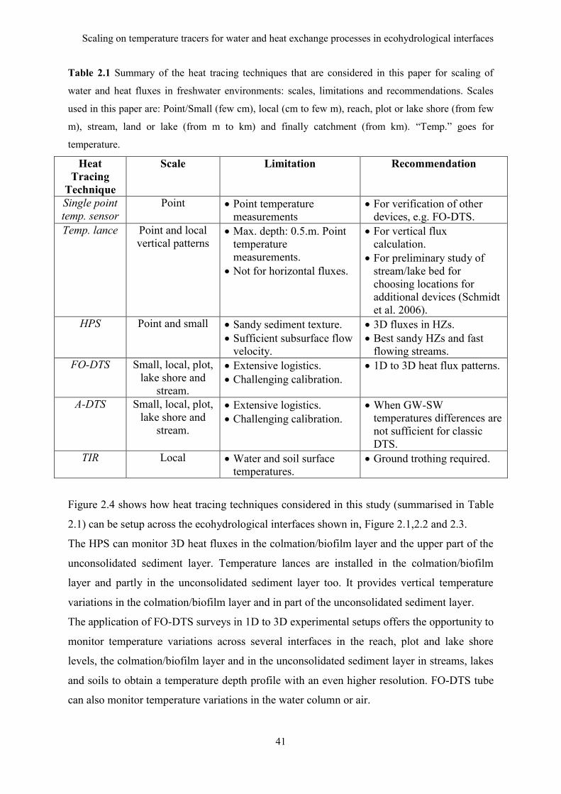
Scaling on temperature tracers for water and heat exchange processes in ecohydrological interfaces
41
Table 2.1 Summary of the heat tracing techniques that are considered in this paper for scaling of
water and heat fluxes in freshwater environments: scales, limitations and recommendations. Scales
used in this paper are: Point/Small (few cm), local (cm to few m), reach, plot or lake shore (from few
m), stream, land or lake (from m to km) and finally catchment (from km). “Temp.” goes for
temperature.
Heat
Tracing
Technique
Scale Limitation Recommendation
Single point
temp. sensor
Point Point temperature
measurements
For verification of other
devices, e.g. FO-DTS.
Temp. lance Point and local
vertical patterns Max. depth: 0.5.m. Point
temperature
measurements.
Not for horizontal fluxes.
For vertical flux
calculation.
For preliminary study of
stream/lake bed for
choosing locations for
additional devices (Schmidt
et al. 2006).
HPS Point and small Sandy sediment texture.
Sufficient subsurface flow
velocity.
3D fluxes in HZs.
Best sandy HZs and fast
flowing streams.
FO-DTS Small, local, plot,
lake shore and
stream.
Extensive logistics.
Challenging calibration.
1D to 3D heat flux patterns.
A-DTS Small, local, plot,
lake shore and
stream.
Extensive logistics.
Challenging calibration.
When GW-SW
temperatures differences are
not sufficient for classic
DTS.
TIR Local Water and soil surface
temperatures.
Ground trothing required.
Figure 2.4 shows how heat tracing techniques considered in this study (summarised in Table
2.1) can be setup across the ecohydrological interfaces shown in, Figure 2.1,2.2 and 2.3.
The HPS can monitor 3D heat fluxes in the colmation/biofilm layer and the upper part of the
unconsolidated sediment layer. Temperature lances are installed in the colmation/biofilm
layer and partly in the unconsolidated sediment layer too. It provides vertical temperature
variations in the colmation/biofilm layer and in part of the unconsolidated sediment layer.
The application of FO-DTS surveys in 1D to 3D experimental setups offers the opportunity to
monitor temperature variations across several interfaces in the reach, plot and lake shore
levels, the colmation/biofilm layer and in the unconsolidated sediment layer in streams, lakes
and soils to obtain a temperature depth profile with an even higher resolution. FO-DTS tube
can also monitor temperature variations in the water column or air.
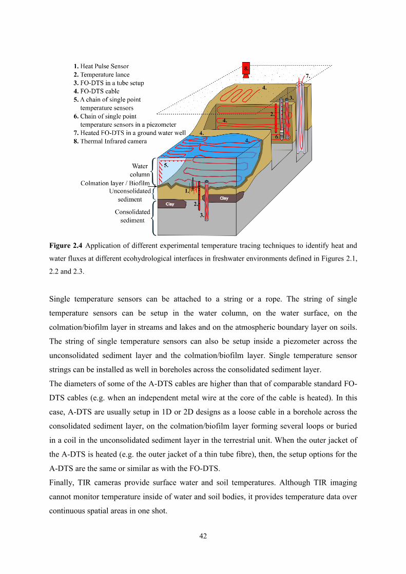
42
Figure 2.4 Application of different experimental temperature tracing techniques to identify heat and
water fluxes at different ecohydrological interfaces in freshwater environments defined in Figures 2.1,
2.2 and 2.3.
Single temperature sensors can be attached to a string or a rope. The string of single
temperature sensors can be setup in the water column, on the water surface, on the
colmation/biofilm layer in streams and lakes and on the atmospheric boundary layer on soils.
The string of single temperature sensors can also be setup inside a piezometer across the
unconsolidated sediment layer and the colmation/biofilm layer. Single temperature sensor
strings can be installed as well in boreholes across the consolidated sediment layer.
The diameters of some of the A-DTS cables are higher than that of comparable standard FO-
DTS cables (e.g. when an independent metal wire at the core of the cable is heated). In this
case, A-DTS are usually setup in 1D or 2D designs as a loose cable in a borehole across the
consolidated sediment layer, on the colmation/biofilm layer forming several loops or buried
in a coil in the unconsolidated sediment layer in the terrestrial unit. When the outer jacket of
the A-DTS is heated (e.g. the outer jacket of a thin tube fibre), then, the setup options for the
A-DTS are the same or similar as with the FO-DTS.
Finally, TIR cameras provide surface water and soil temperatures. Although TIR imaging
cannot monitor temperature inside of water and soil bodies, it provides temperature data over
continuous spatial areas in one shot.

Scaling on temperature tracers for water and heat exchange processes in ecohydrological interfaces
43
Each of the heat tracing techniques included in this paper is generally best used in one
specific scale and phase. However, none of them is able to monitor water and heat fluxes
across the scale continuum and all the ecohydrological interfaces described in Figures 2.1, 2.2
and 2.3.
2.5 Proof of concept: vertical upscaling of discrete GW upwelling by FO-DTS and
TIR
The experimental design and investigation in chapters 3 and 4 are used in the following
section to demonstrate the suitability of the suggested approach for scaling water and heat
exchange processes (Figure 2.3). The triadic structure of hierarchy (Salthe, 1985) was the
basis when designing the experiment approach for tracing warm water up-welling in the
water column caused by discharge of warm GW (LGD). In the present manuscript the term
upwelling describes upward transport processes in the water column. LGD was simulated in
an outdoor mesocosm with injection of warm water at its bottom. In this case, the goal was to
test vertical scaling mechanisms and monitoring technologies across the interfaces of discrete
discharge of warm water, from the colmation/biofilm layer (mesocosm bed) across the water
column to the atmosphere. Thus, our focal level or level 0 was defined as the water column.
The mechanistic understanding of water and heat exchange processes related to LGD comes
from the next lower level or level -1. This belonged to the colmation/biofilm layer (or
mesosom bed) while the relevance of the process is unveiled at the next higher level or level
+1. In the present example, level +1 belongs to the water surface or the water surface-
atmosphere interface.
The processes’ mechanistic understanding (or the main property controlling the processes at
level 0) coming from level -1 can be related to the hydraulic conductivity (K) of the sediment
of the colmation/biofilm layer (or mesocosm bed). Pore-water flow in streambed and lake
bottom sediments is regulated by the hydraulic gradient and the hydraulic conductivity of
sediments while the colmation/biofilm layer adds another filter creating respective spatial
patterns. In the mesocosm experiment of Maruedo et al., 2017, LGD was simulated by a pipe
injecting warm water at the bottom of the mesocosm through a bag filled with coarse
sediments to support dispersion of the point inflow in a more natural way.
The relevance (or impact) of the process can be unveiled on the surface water (or at level +1).
This is understood in terms of how much artificial warm water should be injected in order to
detect a robust heat signal at the water surface. The aim of the experiment was to follow the
heat signal across the water column using different heat tracing techniques at different spatial

44
scales. Going back to Figure 2.4 and having in mind our triadic hierarchical structure we
should follow the figure from right to left within the lake shore level. First we should identify
which are the boundaries and interfaces of our triadic structure in Figure 2.3: Figure 2.5 is a
zoom out of Figure 2.3.
Figure 2.5 Example for vertical scaling of water and heat exchanges related to simulated LGD.
Since there was no colmation/biofilm layer in our case study, the lowest boundary is the
unconsolidated sediment (or the artificial mesocosm bed which is the coarse sediment in the
bag). Which devices could we have deployed on this boundary or interface? If there would
have been a colmation/ biofilm layer, following Figures 2.3 and 2.5, we could have chosen
between a HPS at the small scale and FO-DTS at the local scale. As there was no such layer,
we can substitute the layer by the mesocosm bed compartment (Figure 2.5). Still, the heat
tracing techniques recommended for this interface would be the same. Following Figure 2.5
on the left we find the water column compartment (patch within the lake shore scale level).
Within this compartment measurements can be conducted by using FO-DTS at local scales or
Scaling on temperature tracers for water and heat exchange processes in ecohydrological interfaces
45
single point temperature sensors at point scales. Finally, in Figure 2.5 it is possible to see how
the compartment (patch) called water column overlaps with the element atmosphere. This is
the water column-atmosphere interface. FO-DTS allows measuring at this interface at a local
scale, or – if wanted – at a larger scale (reaching scale). This can be combined with TIR
measurements (see Figure 2.5) at the lake shore scale.
Summarizing, in order to get measurements to trace warm water upwelling across the water
column we could combine the following devices: HPS, single temperature sensors, FO-DTS
and TIR camera. In this way we can get information on small and local scales and at different
interfaces (defined here as vertical scaling).
Since, in this example water discharge is artificial, the injection rate is controlled and the
location of the discrete discharge is known, it was not necessary to monitor the sediment-
water interface. Thus, a 3D setup of FO-DTS cable was used in the water column inside the
mesocosm and a TIR camera was setup at an altitude of 4 m above the mesocosm to monitor
temperature changes caused by upwelling of warm water in the water column (see chapters 3
and 4).
Monitored and analised temperature data showed that at level +1 (water column-atmosphere
interface) the relevance of the process is unveiled (or the effect/impact of the process is
observable), but this was strongly linked to weather conditions. Thus, detectability of warm
water upwelling on the surface water is strongly influenced by weather conditions (see
chapters 3 and 4). Heat fluxes occur across interfaces in both directions: from atmosphere to
the water column and from the water column to the sediment and vice versa. Under clear sky
conditions, downward heat flux from the atmosphere is strong enough to affect and change
the temperature in the water column. In consequence, heat signals from the artificial warm
water upwelling cannot be traced in the top layers of the water column. On the contrary,
under overcast conditions, downward heat flux is not strong enough to affect and change the
temperature in the water column and the heat signal from the artificial warm water upwelling
is possible to be traced in the top layers of the water column (see chapters 3 and 4).
This can be understood in terms of HPD by following definitions of top-down and bottom-up
processes in Poole (2002): Heat fluxes from the atmosphere are strong enough to affect the
condition or the ecological functions (e.g. temperature and consequent change on locations of
thermal refugia for fishes) of the water column compartment (patch) (the water column
conditions change at local and also at small scales) but heat fluxes from the atmosphere can
be affected by changes in patch conditions at much broader scales such as changes in weather
conditions over the catchment (the upper level or scale). This could be defined as a top-down

46
process. Warm water upwelling can be affected by small scale patch structure/functions (e.g.
sediment aggregates, texture, that influence the hydraulic conductivity of the lake bed) but
still can affect patch structure/functions at broader scales (e.g. change in water column
temperature or even reach temperature). This is defined as a bottom-up process (Poole, 2002).
2.6 Synthesis, conclusions and recommendations
In the present paper a conceptual guideline for adequately identify and quantify water and
heat exchange processes and its spatio-temporal variability over several scales and across
ecohydrological interfaces by combination of different heat tracing techniques has been
introduced. The conceptual guideline proposed is based in HPD theory. HPD allows
integrating spatial and temporal variability over several scales and across ecohydrological
interfaces of heat and water exchange processes such us GW-SW exchange processes in lakes
and streams. Figure 2.3 shows the suggestion of applying HPD in freshwater environments
by resolving a generic freshwater environment (or landscape) into different levels or spatial
scales and defining the structural patches that comprise each of the levels. Different heat
tracing techniques are located in the recommended scales (Table 2.1) and ecohydrological
interfaces (Figure 2.4) in order to get the best picture of heat and water exchange processes
over several scales and across ecohydrological interfaces. Finally, as a proof of concept, the
experiment which is described in more detail in chapters 3 and 4, is introduced. This is an
example on how an experimental approach can be designed by following Figure 2.3.
To conclude, the following three main conclusions can be summarized from the work
introduced in the previous sections:
1) Heat exchange processes overlap across spatial and temporal scales and the detection of
heat as a tracer depends on whether the impact or footprint of the investigated process is
dominant or overshadowed:
For instance, in the field of landscape fire ecology, energy fluxes represent processes and
regulations associated with the spatial distribution of energy in relation to patterns in the
landscape (McKenzie et al., 2011). Since the present paper focuses on heat fluxes, process
and pattern definitions used in the field of landscape fire ecology could be followed in the
present case, too. In this manner, heat flux related to water flux is the process that is in our
focal level (Level 0), or focus of interest. But, within ecosystems there are lots of heat fluxes.
Sun radiation is a top down energy input or energy flux. This energetic input is then subjected
to further top-down regulation (e.g. by locally homogeneous spatial fields of humidity,
Scaling on temperature tracers for water and heat exchange processes in ecohydrological interfaces
47
atmospheric pressure, temperatures, and precipitation) (McKenzie et al., 2011). Thus, heat
flux from the atmosphere is a top-down constrain. Whereas, heat flux related to water flux is
a bottom-up process/mechanism. These two heat fluxes will overlap across spatial and
temporal scales.
2) HPD based approach is helpful to distinguish the overlapping impacts of heat transport
processes across spatial and temporal scales:
As found in the example for proof of concept of warm water upwelling tracing experiment,
there is an interaction between top-down and bottom-up heat fluxes across spatial scales.
When top-down heat flux processes dominate over bottom-up mechanistic processes,
homogenizes and coarsens the patterns observed on the surface water (McKenzie et al.,
2011), (e.g. from proof of concept: clear sky conditions allow dominant atmospheric heat
fluxes leading to homogenous warmer surface water in the mesocosm). On the contrary,
when bottom-up processes dominate, more heterogeneous spatial patterns will emerge
(McKenzie et al., 2011) (e.g. from proof of concept: overcast conditions limit heat flux from
the atmosphere and heat fluxes related to warm water upwelling in the mesocosm become
dominant leading to heterogeneous warm water patterns on the water of the mesocosm). Top-
down heat fluxes related to atmospheric conditions can be understood as top-down controls,
or environmental constrains (Urban et al., 1987) over lower levels in the HPD system of a
generic freshwater environment.
3) Introducing HPD into heat tracing across interfaces – this paper used an example
experimental approach from chapters 3 and 4, to successfully demonstrate the
applicability of the HPD concept in experimental approach and method design for
tracing discrete GW upwelling by FO-DTS and TIR across ecohydrological interfaces
(vertical upscaling):
The design and successful application of the experiment based in HPD allowed identification
of top-down (from the atmosphere to the water column) and bottom up (from the source of
the injected warm water in the sediment to the water column) heat fluxes and quantification
of heat fluxes across the water column-atmosphere ecohydrological interface. Identified top-
down processes affected detectability of bottom-up processes such as warm water upwelling
in the water column.
Finally, we would like to remark that it is important to keep in mind that heat fluxes have an
influence over the complete scale continuum and across ecohydrological interfaces and that

48
the used heat tracing techniques will monitor this influence. If we want to identify or isolate
water exchange processes related to LGD, HEF or SW exfiltration by tracing heat fluxes we
first need to know when the heat flux related to those specific processes are dominant over
the spatial and temporal scales and across the interfaces that are being monitored.
Acknowledgments
Funding: This work was supported by the European Union’s Seventh Framework programme
for research, technological development and demonstration [grant number 60715]:
Ecohydrological Interfaces as Critical Hotspots for Transformations of Ecosystem Exchange
Fluxes (INTERFACES).
Supplementary information
Annex S1: Definitions
Graphical abstract

Scaling on temperature tracers for water and heat exchange processes in ecohydrological interfaces
49
References
Ahl V, Timothy F. Allen. 1996. Hierarchy Theory: A Vision, Vocabulary, and Epistemology.
Allen TFH, Starr TB. 1982. Hierarchy: Perspectives for ecological complexity. The
University of Chicago Press: Chicago and London.
Anderson MP. 2005. Heat as a ground water tracer. Ground water 43 (6): 951–68 DOI:
10.1111/j.1745-6584.2005.00052.x
Angermann L, Krause S, Lewandowski J. 2012a. Application of heat pulse injections for
investigating shallow hyporheic flow in a lowland river. Water Resources Research 48
(October): 1–16 DOI: 10.1029/2012WR012564
Angermann L, Lewandowski J, Fleckenstein JH, Nützmann G. 2012b. A 3D analysis
algorithm to improve interpretation of heat pulse sensor results for the determination of
small-scale flow directions and velocities in the hyporheic zone. Journal of Hydrology
475: 1–11 DOI: 10.1016/j.jhydrol.2012.06.050
Baker BH, Martinovic-Weigelt D, Ferrey M, Barber LB, Writer JH, Rosenberry DO, Kiesling
RL, Lundy JR, Schoenfuss HL. 2014. Identifying non-point sources of endocrine active
compounds and their biological impacts in freshwater lakes. Archives of environmental
contamination and toxicology 67 (3): 374–388 DOI: 10.1007/s00244-014-0052-4
Binley A, Ullah S, Heathwaite AL, Heppell C, Byrne P, Lansdown K, Trimmer M, Zhang H.
2013. Revealing the spatial variability of water fluxes at the groundwater-surface water
interface. 49: 3978–3992 DOI: 10.1002/wrcr.20214
Blume T, Krause S, Meinikmann K, Lewandowski J. 2013. Upscaling lacustrine groundwater
discharge rates by fiber-optic distributed temperature sensing. Water Resources
Research 49 (October 2012): 7929–7944 DOI: 10.1002/2012WR013215
Boano F, Harvey JW, Marion A, Packman AI, Revelli R, Ridolfi L, Wörman A. 2014.
Hyporheic flow and transport processes: Mechanisms, models, and bioghemical
implications. Reviews of Geophysics: 1–77 DOI: 10.1002/2012RG000417.Received
Boulton AJ, Findlay S, Marmonier P, Stanley EH, Boulton AJ, Findlay S, Marmonier P,
Stanley EH, Valett HM. 1998. The Functional Significance of the Hyporheic Zone in
Streams and Rivers Maurice Valett Source : Annual Review of Ecology and Systematics
, Vol . 29 ( 1998 ), pp . 59-81 Published by : Annual Reviews Stable URL :
http://www.jstor.org/stable/221702 REFERENC. 29: 59–81
Brabrand Å, Koestler AG, Borgstrøm R. 2002. Lake spawning of brown trout related to
groundwater influx. Journal of Fish Biology 60 (3): 751–763 DOI:
10.1006/jfbi.2002.1901

50
Briggs MA, Buckley SF, Bagtzoglou AC, Werkema DD, Lane JW. 2016. Actively heated
high-resolution fiber-optic-distributed temperature sensing to quantify streambed flow
dynamics in zones of strong groundwater upwelling. 52: 5179–5194 DOI:
10.1002/2015WR018219
Briggs MA, Lautz LK, McKenzie JM, Gordon RP, Hare DK. 2012. Using high-resolution
distributed temperature sensing to quantify spatial and temporal variability in vertical
hyporheic flux. Water Resources Research 48 (2): 1–16 DOI: 10.1029/2011WR011227
Byrne GF, Drummond JE, Rose CW. 1967. A sensor for water flux in soil. ‘Point source’
instrument. Water Resources Research 3 (4): 1073–1078 DOI:
10.1029/WR003i004p01073
Ciocca F, Lunati I, Van de Giesen N, Parlange MB. 2012. Heated Optical Fiber for
Distributed Soil-Moisture Measurements: A Lysimeter Experiment. Vadose Zone
Journal 11 (4): 0 DOI: 10.2136/vzj2011.0199
Constantz J, Stonestrom D a. 2003. Heat as a tracer of water movement near streams. In Heat
as a Tool for Studying the Movement of Ground Water near Streams, Stonestrom DA, ,
Constantz J (eds).Reston, Virginia; 1–6. Available at:
http://pubs.usgs.gov/circ/2003/circ1260/#pdf
Cuthbert MO, Mackay R, Durand V, Aller MF, Greswell RB, Rivett MO. 2010. Impacts of
river bed gas on the hydraulic and thermal dynamics of the hyporheic zone. Advances in
Water Resources 33 (11): 1347–1358 DOI: 10.1016/j.advwatres.2010.09.014
Davies AG, Calkins J, Scharenbroich L, Vaughan RG, Wright R, Kyle P, Castańo R, Chien
S, Tran D. 2008. Multi-instrument remote and in situ observations of the Erebus
Volcano (Antarctica) lava lake in 2005: A comparison with the Pele lava lake on the
jovian moon Io. Journal of Volcanology and Geothermal Research 177 (3): 705–724
DOI: 10.1016/j.jvolgeores.2008.02.010
Dent CL, Grimm NB, Fisher SG. 2001. Multiscale effects of surface-subsurface exchange on
stream water nutrient concentrations. Journal of the North American Benthological
Society 20 (2): 162–181 DOI: 10.2307/1468313
Fisher SG, Grimm NB, Marti E, Gomez R. 1998. Hierarchy, spatial configuration, and
nutrient cycling in a desert stream. Australian Journal of Ecology 23 (1): 41–52 DOI:
10.1111/j.1442-9993.1998.tb00704.x
Forman RTT. 1995. Some general principles of landscape and regional ecology. Landscape
Ecology 10 (3): 133–142 DOI: 10.1007/BF00133027
Frissell CA, Liss WJ, Warren CE, Hurley MD. 1986. A hierarchical framework for stream

Scaling on temperature tracers for water and heat exchange processes in ecohydrological interfaces
51
habitat classification: Viewing streams in a watershed context. Environmental
Management 10 (2): 199–214 DOI: 10.1007/BF01867358
Goldstein J. 1999. Emergence as a Construct: History and Issues. 1: 49–72 DOI:
10.1207/s15327000em0101_4
Gordon RP, Lautz LK, Briggs MA, McKenzie JM. 2012. Automated calculation of vertical
pore-water flux from field temperature time series using the VFLUX method and
computer program. Journal of Hydrology 420–421: 142–158 DOI:
10.1016/j.jhydrol.2011.11.053
Greswell RB, Riley MS, Alves PF, Tellam JH. 2009. A heat perturbation flow meter for
application in soft sediments. Journal of Hydrology 370 (1–4): 73–82 DOI:
10.1016/j.jhydrol.2009.02.054
Haghighi E, Or D. 2015. Thermal signatures of turbulent airflows interacting with
evaporating thin porous surfaces. International Journal of Heat and Mass Transfer 87:
429–446 DOI: 10.1016/j.ijheatmasstransfer.2015.04.026
Hare DK, Briggs MA, Rosenberry DO, Boutt DF, Lane JW. 2015. A comparison of thermal
infrared to fiber-optic distributed temperature sensing for evaluation of groundwater
discharge to surface water. Journal of Hydrology 530: 153–166 DOI:
10.1016/j.jhydrol.2015.09.059
Hayashi M, Rosenberry D. 2002. Effects of Ground Water Exchange on the Hydrology and
Ecology of Surface Water. Ground Water 40 (3): 309–316
Johnson LB, Gage SH. 1997. Landscape approaches to the analysis of aquatic ecosystems.
Freshwater Biology 37: 113–132 DOI: 10.1046/j.1365-2427.1997.00156.x
Kawanishi H. 1983. A soil-water flux sensor and its use for field studies of transfer processes
in surface soil. Journal of Hydrology 60 (1–4): 357–365 DOI: 10.1016/0022-
1694(83)90031-8
Koestler AG. 1967. The ghost in the machine.
Krause S, Blume T, Cassidy NJ. 2012. Investigating patterns and controls of groundwater up-
welling in a lowland river by combining Fibre-optic Distributed Temperature Sensing
with observations of vertical hydraulic gradients. Hydrology and Earth System Sciences
16 (6): 1775–1792 DOI: 10.5194/hess-16-1775-2012
Krause S, Boano F, Cuthbert MO, Fleckenstein JH, Lewandowski J. 2014. Understanding
process dynamics at aquifer-surface water interfaces: An introduction to the special
section on new modeling approaches and novel experimental technologies: Introduction.
Water Resources Research 50 (2): 1847–1855 DOI: 10.1002/2013WR014755

52
Krause S, Lewandowski J, Grimm NB, Hannah DM, Pinay G, Mcdonald K, Martí E,
Argerich A, Pfister L, Klaus J, et al. 2017. Ecohydrological interfaces as hotspots of
ecosystem processes. Water Resources Research DOI: 10.1002/2016WR019516
Krause S, Taylor SL, Weatherill J, Haffenden A, Levy A, Cassidy NJ, Thomas PA. 2013.
Fibre-optic distributed temperature sensing for characterizing the impacts of vegetation
coverage on thermal patterns in woodlands. Ecohydrology 6 (5): 754–764 DOI:
10.1002/eco.1296
Lautz LK, Ribaudo RE. 2012. Scaling up point-in-space heat tracing of seepage flux using
bed temperatures as a quantitative proxy. Hydrogeology Journal 20 (7): 1223–1238
DOI: 10.1007/s10040-012-0870-2
Lee E, Kang K, Hyun SP, Lee K-Y, Yoon H, Kim SH, Kim Y, Xu Z, Kim D, Koh D-C, et al.
2016. Submarine groundwater discharge revealed by aerial thermal infrared imagery: a
case study on Jeju Island, Korea. Hydrological Processes 3506 (June): 3494–3506 DOI:
10.1002/hyp.10868
Lewandowski J, Angermann L, Nützmann G, Fleckenstein JH. 2011. A heat pulse technique
for the determination of small-scale flow directions and flow velocities in the streambed
of sand-bed streams. Hydrological Processes 25 (March): 3244–3255 DOI:
10.1002/hyp.8062
Lewandowski J, Meinikmann K, Ruhtz T, Pöschke F, Kirillin G. 2013. Localization of
lacustrine groundwater discharge (LGD) by airborne measurement of thermal infrared
radiation. Remote Sensing of Environment 138: 119–125 DOI:
10.1016/j.rse.2013.07.005
Lowry CS, Walker JF, Hunt RJ, Anderson MP. 2007. Identifying spatial variability of
groundwater discharge in a wetland stream using a distributed temperature sensor. Water
Resources Research 43 (10): n/a-n/a DOI: 10.1029/2007WR006145
McBride MS, Pfannkuch HO. 1975. The distribution of seepage within lakebeds. Journal of
Research of the U.S. Geological Survey 3 (5): 505–512 Available at:
http://scholar.google.com/scholar?hl=en&btnG=Search&q=intitle:Revised+Value+for+t
he+O18+Fractionation+Between+CO2+and+H2O+at+25#0
Mcdonnell JJ, Sivapalan M, Vache K, Dunn S, Grant G, Haggerty R. 2007. Moving beyond
heterogeneity and process complexity : A new vision for watershed hydrology. 43: 1–6
DOI: 10.1029/2006WR005467
McKenzie D, Miller C, Falk DA. 2011. The Landscape Ecology of Fire (D McKenzie, C
Miller, and DA Falk, eds). Springer Netherlands. DOI: 10.1007/978-94-007-0301-8
Scaling on temperature tracers for water and heat exchange processes in ecohydrological interfaces
53
Meinikmann K, Lewandowski J, Nützmann G. 2013. Lacustrine groundwater discharge:
Combined determination of volumes and spatial patterns. Journal of Hydrology 502:
202–211 DOI: 10.1016/j.jhydrol.2013.08.021
Nakayama T, Watanabe M. 2008. Missing role of groundwater in water and nutrient cycles in
the shallow eutrophic Lake Kasumigaura, Japan. Hydrological Processess 22: 1150–
1172 DOI: 10.1002/hyp.6684
O’Neill RV, Johnson AR, King AW. 1989. A hierarchical framework for the analysis of
scale*. Landscape Ecology 3 (3381): 193–205
Poole GC. 2002. Fluvial landscape ecology: Addressing uniqueness within the river
discontinuum. Freshwater Biology 47 (4): 641–660 DOI: 10.1046/j.1365-
2427.2002.00922.x
Poole GC, Berman CH. 2001. An Ecological Perspective on In-Stream Temperature : Natural
Heat Dynamics and Mechanisms of Human-Caused Thermal Degradation. 27 (6): 787–
802 DOI: 10.1007/s002670010188
Pöschke F, Lewandowski J, Engelhardt C, Preuß K, Oczipka M, Ruhtz T, Kirillin G. 2015.
Upwelling of deep water during thermal stratification onset—Amajormechanismof
vertical transport in small temperate lakes in spring? Water Resources Research 51
(January 2016): 9612–9627 DOI: 10.1002/2015WR017579
Read T, Bour O, Selker JS, Bense VF, Le Borgne T, Hochreutener R, Lavenant N. 2014.
Active-Distributed Temperature Sensing to continuously quantify vertical flow in
boreholes. Water Resources Research 50: 3706–3713 DOI: 10.1002/2014WR015273
Ren T, Kluitenberg GJ, Horton R. 2000. Determining Soil Water Flux and Pore Water
Velocity by a Heat Pulse Technique. Soil Science Society of America Journal 64 (2):
552–560 DOI: 10.2136/sssaj2000.642552x
Salthe SN. 1985. Evolving hierarchical systems: Their structure and representation.
Columbia University Press: New York.
Schmidt C, Bayer-Raich M, Schirmer M. 2006. Characterization of spatial heterogeneity of
groundwater-stream water interactions using multiple depth streambed temperature
measurements at the reach scale. Hydrology and Earth System Sciences Discussions 3
(4): 1419–1446
Selker JS, van de Giesen N, Westhoff M, Luxemburg W, Parlange MB. 2006a. Fiber optics
opens window on stream dynamics. Geophysical Research Letters 33 (24): L24401
DOI: 10.1029/2006GL027979
Selker JS, Thévenaz L, Huwald H, Mallet A, Luxemburg W, van de Giesen N, Stejskal M,

54
Zeman J, Westhoff M, Parlange MB. 2006b. Distributed fiber-optic temperature sensing
for hydrologic systems. Water Resources Research 42 (12): n/a-n/a DOI:
10.1029/2006WR005326
Shaw RD, Shaw JFH, Fricker H, Prepas EE. 1990. An integrated approach to quantify
groundwater transport of phosphorus to Narrow Lake , Alberta. 35 (4): 870–886
Simon HA. 1977. The Organization of Complex Systems. In Models of Discovery: And Other
Topics in the Methods of ScienceSpringer Netherlands: Dordrecht; 245–261. DOI:
10.1007/978-94-010-9521-1_14
Simon HA. 1997. The sciences of the artificial, (third edition). DOI: 10.1016/S0898-
1221(97)82941-0
Soranno PA, Webster KE, Cheruvelil KS, Bremigan MT. 2009. The lake landscape-context
framework : linking aquatic connections , terrestrial features and human effects at
multiple spatial scales. Verh. Internat. Verein. Limnol. 30 (January): 695–700
Soranno P a., Cheruvelil KS, Webster KE, Bremigan MT, Wagner T, Stow C a. 2010. Using
Landscape Limnology to Classify Freshwater Ecosystems for Multi-ecosystem
Management and Conservation. BioScience 60 (6): 440–454 DOI:
10.1525/bio.2010.60.6.8
Timothy F. Allen. A summary of the principles of hierarchy theory Available at:
http://www.isss.org/hierarchy.htm
Turner MG. 1989. Landscape Ecology: The Effect of Pattern on Process. Annual Review of
Ecology and Systematics 20 (1): 171–197 DOI: 10.1146/annurev.es.20.110189.001131
Urban DL, Neill RVO, Shugart HH. 1987. Ecology Landscape spatial patterns. BioScience 37
(2): 119–127
Warren DR, Sebestyen SD, Josephson DC, Lepak JM, Kraft CE. 2005. Acidic Groundwater
Discharge and in Situ Egg Survival in Redds of Lake-Spawning Brook Trout.
Transactions of the American Fisheries Society 134 (5): 1193–1201 DOI: 10.1577/T04-
180.1
Wawrzyniak V, Piégay H, Allemand P, Vaudor L, Goma R, Grandjean P. 2016. Effects of
geomorphology and groundwater level on the spatio-temporal variability of riverine cold
water patches assessed using thermal infrared (TIR) remote sensing. Remote Sensing of
Environment 175: 337–348 DOI: 10.1016/j.rse.2015.12.050
Wu J. 1999. Hierarchy and scaling: extrapolating information along a scaling ladder.
Canadian Journal of Remote Sensing 25 (4): 367–380
Wu J. 2013. Hierarchy Theory: An Overview. In Linking Ecology and Ethics for a Changing
Scaling on temperature tracers for water and heat exchange processes in ecohydrological interfaces
55
World: Values, Philosophy, and Action, Rozzi R, , Pickett STA, , Palmer C, , Armesto
JJ, , Callicott JB (eds).Springer Netherlands: Dordrecht; 281–301. DOI: 10.1007/978-
94-007-7470-4_24
Wu J, David JL. 2002. A spatially explicit hierarchical approach to modeling complex
ecological systems : theory and applications. 153: 7–26
Wu J, Levin SA. 1997. A patch-based spatial modeling approach : conceptual framework and
simulation scheme. 101: 325–346
Wu J, Loucks OL. 1995. From Balance of Nature to Hierarchical Patch Dynamics : A
Paradigm Shift in Ecology. The quarterly review of biology 70 (4): 439–466 DOI: 0033-
5770/95/7004-0003
Annex S1: Definitions
System: Any interacting, interdependent or associated group of entities.
Context: set of circumstances and facts that surround particular event or situation.
Systems’ context: encompassing element structure (Poole, 2002).
Hierarchy: Any system of things ranked one above another.
Hierarchic system: system formed by interrelated subsystems (Simon, 1997).
Entity: component (O’Neill et al. 1989) or subsystem.
Levels: A section of a hierarchy which is defined by a scale (Allen and Starr 1982, 1996).
Within a level there are entities whose features characterize the level they are part of. An
entity can belong to any amount of levels depending on the criteria used to unite levels above
and below (Timothy F. Allen).
Scalar hierarchy: Empirically based levels of observations (Ahl and Timothy F. Allen,
1996).
Definitional hierarchy: Observer defined level of organization (Ahl and Timothy F. Allen,
1996).
Scalar levels: in a scalar hierarchy.
Definitional levels: in a definitional hierarchy.
Patch: Basic homogeneous unit observable in the landscape at a certain spatial scale. A patch
can change its dynamic, structure, arrangement, union or function (Poole, 2002). Patch might
be analog to entity, subsystem, Holon, component or part. These terms are commonly used in
Hierarchy Theory.
Processes: Water and heat exchange processes.
Trans-scale: across scales.

56
Trans-interface: across interfaces.
Elements: Patches, parts of the system.
System elements: system patches.
Structural elements: Structural patches.
Element’s ecological function: Patch’s ecological function (Poole, 2002).
A landscape: A dynamic interaction of terrestrial and aquatic elements/patches (Forman,
1995).
Top-down process: They influence the internal structure of the system. Processes influence
by patch function/condition at coarse scales but influences patch function/condition at finer
scales (Poole, 2002).
Top-down constrains/influences: e.g. Environmental constrains. Each of the constrains
provides a context for the behaviors of the lower levels of the hierarchy (Urban et al., 1987;
Wu, 2013).
Bottom up process: Processes are influenced by fine scale patch’s function/condition but
influence patch function/conditions at coarser scales (Poole, 2002).
Bottom up mechanism: initiating forces at lower levels of the hierarchy (Wu 2013).
Emergent properties: properties that emerge via collective actions of many individual
entities. Arise of a novel and coherent structures, patterns and properties during the process of
self-organization in complex systems (Goldstein, 1999).
Holon: Subsystem that comprise a level (Koestler, 1967).
Interface: Surface regarded as common boundary of two spaces, phases.
Compartment: Phase= bodies, spaces.
Sister Holon: two communicating Holon which occur at the same level in a hierarchy and do
not exert constrain over each other (Allen and Starr 1982).
Interactions among Holons of same level are symmetric, among components within a
Holon are stronger and more frequent than those among Holons (Koestler, 1967; Allen and
Starr, 1982).
In HPD and patch dynamics, patch refers to the term Holon which is used in hierarchy
theory.
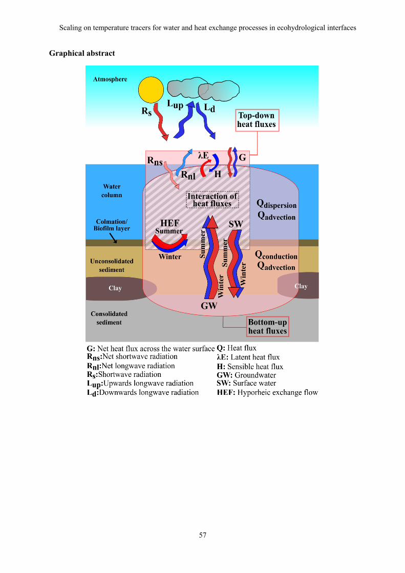
Scaling on temperature tracers for water and heat exchange processes in ecohydrological interfaces
57
Graphical abstract

58
3 Mesocosm experiments identifying hotspots of groundwater upwelling in a water
column by fiber optic distributed temperature sensing
Amaya I. Marruedo Arricibitaa,b
, Stefan Krausec, Jesus Gomez-Velez
d, David M. Hannah
c
and Jörg Lewandowskia,b
a Department of Ecohydrology, Leibniz-Institute of Freshwater Ecology and Inland Fisheries,
12587 Berlin, Germany.
b Department of Geography, Humboldt University of Berlin, 10099 Berlin, Germany.
c School of Geography, Earth and Environmental Sciences, University of Birmingham, B15
2TT Birmingham, United Kingdom.
d Department of Earth and Environmental Science, New Mexico Institute of Mining &
Technology, Socorro, NM 87801; United States.
Published in: Hydrological Processes
Marruedo Arricibita AI, Krause S, Gomez-Velez J, Hannah DM, Lewandowski J. 2018.
Mesocosm experiments identifying hotspots of groundwater upwelling in a water column by
fibre optic distributed temperature sensing. Hydrological Processes 32 (2): 185–199 DOI:
10.1002/hyp.11403
This is an open access article under the terms of the Creative Commons Attribution License,
which permits use, distribution and reproduction in any medium, provided the original work
is properly cited.
© 2017 The Authors. Hydrological Processes Published by John Wiley & Sons Ltd.

Mesocosm experiments identifying hotspots of groundwater upwelling in a water column by fiber
optic distributed temperature sensing
59
Abstract
Lacustrine groundwater discharge (LGD) can substantially impact ecosystem characteristics
and functions. Fibre optic distributed temperature sensing (FO‐DTS) has been successfully
used to locate groundwater discharge into lakes and rivers at the sediment–water interface,
but locating groundwater discharge would be easier if it could be detected from the more
accessible water surface. So far, it is not clear if how and under which conditions the LGD
signal propagates through the water column to the water surface–atmosphere interface, and
what perturbations and signal losses occur along this pathway. In the present study, LGD was
simulated in a mesocosm experiment. Under winter conditions, water with temperatures of 14
to 16 °C was discharged at the bottom of a 10 × 2.8‐m mesocosm. Water within this
mesocosm ranged from 4.0 to 7.4 °C. Four layers (20, 40, 60, and 80 cm above the sediment)
of the 82 cm deep mesocosm were equipped with FO‐DTS for tracing thermal patterns in
the mesocosm. Aims are (a) to test whether the positive buoyancy of relatively warm
groundwater imported by LGD into shallow water bodies allows detection of LGD at the
lake's water surface–atmosphere interface by FO‐DTS, (b) to analyse the propagation of the
temperature signal from the sediment‐water interface through the water column, and (c) to
learn more about detectability of the signal under different discharge rates and weather
conditions. The experiments supported the benchmarking of scale dependencies and
robustness of FO‐DTS applications for measuring upwelling into aquatic environments and
revealed that weather conditions can have important impacts on the detection of upwelling at
water surface–atmosphere interfaces at larger scales.
Keywords
lake, FO‐DTS, heat tracer, jet, interface, driver

60
3.1 Introduction
Lacustrine groundwater discharge (LGD), that is, the discharge of groundwater (GW) into
lakes, can substantially impact ecosystem characteristics and functions (Baker et al., 2014;
Ridgway & Blanchfield, 1998; Warren, Sebestyen, Josephson, Lepak, & Kraft, 2005).
Upwards directed GW flow is sometimes called upwelling, especially in the context of
hyporheic zones, where commonly both upwelling and downwelling occur along river
reaches. In the present manuscript, we use the term upwelling solely for upward transport
processes in the water column; this definition is adopted from limnophysics. On the one hand,
upwelling of warm water in cold lakes can be caused by natural processes such as GW flow
across the lake bed into the cold lake water body during winter conditions (LGD;
Lewandowski, Meinikmann, Ruhtz, Pöschke, & Kirillin, 2013) or thermal springs in volcanic
lakes (Cardenas et al., 2012). On the other hand, it can be related to thermal pollution caused
by industries such as electric power plants, which use water and discharge heated water into
lakes and streams (Hung, Eldridge, Taricska, & Li, 2005; Shuster, 1986). In both cases,
quantitative interpretations of warm water upwelling patterns are hampered by the lack of
understanding of how the signal propagates from the sediment–water interface through the
water column to the water surface–atmosphere interface and which perturbations and signal
losses occur along this pathway. The present study will focus on LGD as an example of
upwelling of warm water in lacustrine ecosystems during winter conditions due to its
substantial impact on the ecosystem characteristics and functioning. LGD creates favourable
habitats by affecting water chemical composition and temperature, supporting for instance the
spawning of fish (Brunke & Gonser, 1997; Hayashi & Rosenberry, 2002). As climate warms,
aquatic environments with strong GW influence are expected to support habitat stability and
provide refuge for thermally stressed‐aquatic species (Brabrand, Koestler, & Borgstrøm,
2002; Curry & Noakes, 1995; Hayashi & Rosenberry, 2002). Furthermore, detection of LGD
is essential with respect to identifying it as a potential vector for pollution in aquatic
ecosystems when GW quality is degraded (Nakayama & Watanabe, 2008). Despite the
reported relevance of LGD on ecosystems, very little has been written about discharge of
warm GW to lakes. Nearly all of the literature discusses discharge of cold GW to warm lakes,
primarily because most of the research has been conducted during warm‐water periods.
Relatively cold GW has a higher density than warm lake water and, thus, would not reach the
water surface.
There are no detailed field observations of how warm water propagates through the water
column and to the surface of the lake during winter conditions. We address this research gap

Mesocosm experiments identifying hotspots of groundwater upwelling in a water column by fiber
optic distributed temperature sensing
61
by looking at trigger conditions that allow upwelling of LGD from the sediment–water
interface to the water surface atmosphere interface. We consider the temperature difference
required between GW and surface water (SW) as well as the influence of meteorological
conditions and diurnal cycles. The different temperatures of GW and SW might allow the
detection of potential discrete areas of GW discharge to SW (Hare, Briggs, Rosenberry,
Boutt, & Lane, 2015). Under the prerequisite of similar ion composition (which impacts
water density), warm GW is less dense and more buoyant than cold SW, which allows
upwelling of GW to the water surface. Thus, heat convection is augmented by density driven
buoyant forces where warm GW discharges to cold SW. This process occurs during winter
and early spring when SW is substantially colder than discharging GW and when the mixing
is at a minimum at the lake surface (Hare et al., 2015; Lewandowski et al., 2013).
The basic concept of fibre optic distributed temperature (FO‐DTS) technology is to analyse
the temperatures monitored along specific distance intervals of a fibre optic cable based on
(a) the travelling time of light in the optic fibre and (b) the temperature‐dependent
backscattering of light in the fibre (Selker, van de Giesen, Westhoff, Luxemburg, & Parlange,
2006). In this way, temperature can be monitored through the fibre optic cable up to a
distance of several km, with spatial resolutions ranging from 0.3 to 4 m and measurement
precision of 0.05 to 0.1 °C when sampling over 30‐s intervals (Hausner et al., 2011; Selker,
Thévenaz, et al., 2006; van de Giesen et al., 2012). FO‐DTS has been used to detect GW
discharge at the sediment–water interface of lakes (Blume, Krause, Meinikmann, &
Lewandowski, 2013; Liu, Liu, Wang, & Zheng, 2015; Sebok et al., 2013) and streams
(Krause, Blume, & Cassidy, 2012; Lowry, Walker, Hunt, & Anderson, 2007). Here, FO‐DTS
is placed in layers of a specific depth above the sediment–water interface, to provide high‐
resolution temperature data to quantify the incidence, frequency, persistence, and attenuation
of warmer discharging GW that reaches the water surface.
The aim of this study is to show that during winter, the positive buoyancy of relatively warm
LGD to cold SW will allow or enhance detection of GW at the water surface–atmosphere
interface (the lake surface). To address this aim, a mesocosm was used as a model system.
Different layers of FO‐DTS cable were deployed at different water depths to measure the
temperature distribution. In addition, the following questions are addressed:
1. Which lake‐internal upwelling patterns from the sediment–water interface through the
water column to the water surface–atmosphere interface are caused by (simulated)
LGD?
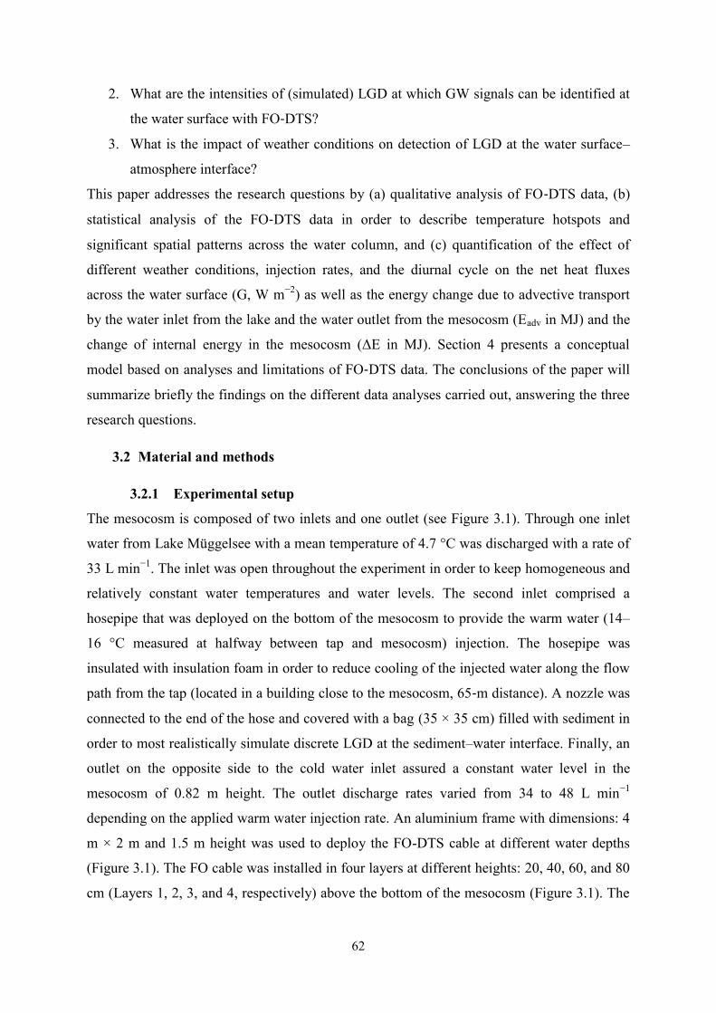
62
2. What are the intensities of (simulated) LGD at which GW signals can be identified at
the water surface with FO‐DTS?
3. What is the impact of weather conditions on detection of LGD at the water surface–
atmosphere interface?
This paper addresses the research questions by (a) qualitative analysis of FO‐DTS data, (b)
statistical analysis of the FO‐DTS data in order to describe temperature hotspots and
significant spatial patterns across the water column, and (c) quantification of the effect of
different weather conditions, injection rates, and the diurnal cycle on the net heat fluxes
across the water surface (G, W m−2
) as well as the energy change due to advective transport
by the water inlet from the lake and the water outlet from the mesocosm (Eadv in MJ) and the
change of internal energy in the mesocosm (ΔE in MJ). Section 4 presents a conceptual
model based on analyses and limitations of FO‐DTS data. The conclusions of the paper will
summarize briefly the findings on the different data analyses carried out, answering the three
research questions.
3.2 Material and methods
3.2.1 Experimental setup
The mesocosm is composed of two inlets and one outlet (see Figure 3.1). Through one inlet
water from Lake Müggelsee with a mean temperature of 4.7 °C was discharged with a rate of
33 L min−1
. The inlet was open throughout the experiment in order to keep homogeneous and
relatively constant water temperatures and water levels. The second inlet comprised a
hosepipe that was deployed on the bottom of the mesocosm to provide the warm water (14–
16 °C measured at halfway between tap and mesocosm) injection. The hosepipe was
insulated with insulation foam in order to reduce cooling of the injected water along the flow
path from the tap (located in a building close to the mesocosm, 65‐m distance). A nozzle was
connected to the end of the hose and covered with a bag (35 × 35 cm) filled with sediment in
order to most realistically simulate discrete LGD at the sediment–water interface. Finally, an
outlet on the opposite side to the cold water inlet assured a constant water level in the
mesocosm of 0.82 m height. The outlet discharge rates varied from 34 to 48 L min−1
depending on the applied warm water injection rate. An aluminium frame with dimensions: 4
m × 2 m and 1.5 m height was used to deploy the FO-DTS cable at different water depths
(Figure 3.1). The FO cable was installed in four layers at different heights: 20, 40, 60, and 80
cm (Layers 1, 2, 3, and 4, respectively) above the bottom of the mesocosm (Figure 3.1). The
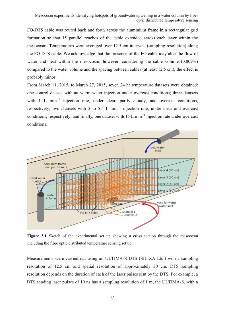
Mesocosm experiments identifying hotspots of groundwater upwelling in a water column by fiber optic distributed temperature sensing
63
FO-DTS cable was routed back and forth across the aluminium frame in a rectangular grid
formation so that 15 parallel reaches of the cable extended across each layer within the
mesocosm. Temperatures were averaged over 12.5 cm intervals (sampling resolution) along
the FO-DTS cable. We acknowledge that the presence of the FO cable may alter the flow of
water and heat within the mesocosm; however, considering the cable volume (0.009%)
compared to the water volume and the spacing between cables (at least 12.5 cm), the effect is
probably minor.
From March 11, 2015, to March 27, 2015, seven 24 hr temperature datasets were obtained:
one control dataset without warm water injection under overcast conditions; three datasets
with 1 L min−1 injection rate, under clear, partly cloudy, and overcast conditions,
respectively; two datasets with 5 to 5.5 L min−1 injection rate, under clear and overcast
conditions, respectively; and finally, one dataset with 15 L min−1 injection rate under overcast
conditions.
Figure 3.1 Sketch of the experimental set up showing a cross section through the mesocosm
including the fibre optic distributed temperature sensing set up.
Measurements were carried out using an ULTIMA-S DTS (SILIXA Ltd.) with a sampling
resolution of 12.5 cm and spatial resolution of approximately 30 cm. DTS sampling
resolution depends on the duration of each of the laser pulses sent by the DTS. For example, a
DTS sending laser pulses of 10 ns has a sampling resolution of 1 m, the ULTIMA-S, with a

64
sampling resolution of 12.5 cm, sends pulses of 1.25 ns. The spatial resolution refers to the
distance between points along the FO cable located next to an abrupt change on temperature
in a way that the point on the low side is not placed higher than 10% of the abrupt jump and
the point on the high side is placed higher than 90% of the abrupt jump (Selker, Tyler, & Van
de Giesen, 2014). Five hundred metres of multimode FO cable from Silixa Ltd., were
deployed for the experiments of this study. Using a multimode fibre allowed flexible bending
and thus supported an adequate set up of the cable in the aluminium frame.
Simulated upwelling flux rates versus rates reported in literature
The LGD rates used in the present study are based on measured flow rates in the tube (1 to 15
L min−1
) used for injecting warm water into the mesocosm. The tube outlet is covered by a
sand bag to simulate discrete LGD from sediments. An uncovered tube outlet might have
caused a jet stream that would be quite unrealistic for LGD and therefore was avoided. The
LGD rate can be referred to different areas: (a) the sand bag covering the tube outlet (35 × 35
cm) resulting in 8.2 to 122.4 L m−2
min−1
, (b) a square metre, that is, 1 to 15 L m−2
min-1
, and
(c) the entire mesocosm (10 × 2.8 × 0.82 m) resulting in 0.036 to 0.536 L m−2
min−1
. The
latter approach is often used in lake studies in which the total exfiltration is related to the
entire lakebed.
The LGD rates applied in the present mesocosm experiment are at the upper end of LGD
rates occurring in situ. Rosenberry, Lewandowski, Meinikmann, and Nützmann (2015)
reviewed the international literature and report a median exfiltration rate of 0.74 cm day−1
(=0.005 L m−2
min−1
) and a maximum of 745 cm day−1
(=5.2 L m−2
min−1
). The maximum of
745 cm day−1
is a point estimate based on seepage metre measurements (Kidmose,
Engesgaard, Nilsson, Laier, & Looms, 2011). A high rate referred to the entire lake bed is
reported by Piña-Ochoa and Lvarez-Cobelas (2009), which is 0.05 to 0.1 L m−2
day−1
. For
punctual focused LGD much higher rates are possible: For example, in Norrström and Jacks
(1996) macropore GW discharge rates of 18 and 42 L min−1
are reported for areas of 0.0078
and 0.031 m2. More extreme examples can be found in natural thermal ponds or pools with
hot springs with up to 800 L min−1
discharge rates (Haselwimmer, Prakash, & Holdmann,
2013). Intense warm water discharge might also be of anthropogenic origin such as sewage
leakage from under water pipes (Apperl, Pressl, & Schulz, 2017).
Measurement protocol and calibration
Once the FO cable was properly deployed onto the aluminium frame, the exact start and end
positions of each cable line were identified.
Mesocosm experiments identifying hotspots of groundwater upwelling in a water column by fiber
optic distributed temperature sensing
65
This was done by locally warming the cable at each bend, identifying the temperature peak on
the data output graph, and noting the distance along the cable at this peak. This allowed
locating of each of the four fibre optic layers, including their start and end points, as well as
the beginning and end of each FO cable sequence.
Calibration of the FO‐DTS by temperature offset correction was carried out using an external
probe of the DTS device and FO cable reference sections within an isolated ice bath with a
mix of ice and water that assured constantly 0 °C. For the differential loss correction, the
fixed value setting was chosen along the relatively short cable (500 m) without any splices. A
default value of 0.255 dB/km was used as this value is the expected value for Corning
ClearCurve™ OM3 fibre.
An alternate single‐ended measurement set up was used with alternating monitoring direction
of the light pulse sent from the DTS device. Measurements were averaged at 10‐s intervals
(integration time) in each direction. This means that the time interval between measurements
from the same channel was 20 s.
3.2.2 Data analyses and spatial statistics
All data analysis, including summarizing statistics for quantification of spatial patterns and
statistical relationships of observed data within layers and between layers, was conducted in
R and ArcGIS. The following spatial statistical metrics were quantified:
Moran’s I and Moran Scatter Plot of testing spatial autocorrelation
The Moran's I values were calculated as indicators of the degree of linear association between
a value in a specific location (x-axis) and surrounding locations (y-axis). Moran's I scatter
plots were used to visualize the type and strength of spatial autocorrelation of observed
temperatures. The four quadrants of the Moran's I scatter plot indicate, from x-axis to y-axis:
high-high and low-low quadrants contain values with positive spatial autocorrelation and
high-low and low-high quadrants contain values with negative spatial autocorrelations. The
Moran's I scatter plot displays a “spatially lagged” transformation of a variable (in y-axis) on
the original spatial variable (in x-axis). In addition, the Moran's I scatter plot reports the
summary of potential influential observations (highlighted in red diamond shape in Moran's I
scatter plot) for the linear relationship between the data and the lag. Finally, the slope of the
scatter plot indicates Moran's I values obtained and the overall spatial autocorrelation of the
dataset (Anselin, 1996; Bivand, Pebesma, & Gómez-Rubio, 2013).

66
Local Indicators of Spatial Association maps
Local indicators of spatial association (LISA) have been calculated to identify significant
spatial clusters or outliers that have been used in this study to highlight local hotspots of
simulated warm water upwelling. The clusters and spatial outliers of LISA maps correspond
to the four quadrants of the Moran's I scatter plots, providing a measure of clusters or outliers
that are of statistical significance (Anselin, 1995).
Spatial correlation between layers: Band collection statistics
Band collection statistics conducted in AcrGIS allowed the analysis of sets of raster bands, in
the present study a set of 4 FO-DTS temperature layers. Covariance and correlation matrices
and basic statistical parameters (minimum, maximum, mean, and standard deviation) for each
layer have been calculated. The covariance matrix indicates for each layer how much
variance is from the mean value of each layer. The correlation matrix shows how correlated
the cell values of one layer are to the cell values of another layer (Environmental Systems
Research Institute, 2014).
3.2.3 Preprocessing and sources of error
Figure 3.2a shows temperature data of a single measurement point on the FO cable over 24 hr
of measurement (black line) with a clear diurnal trend. However, noise is predominant on the
plotted curve. Noise can be related to the sensor, turbulence, and short time fluctuations of
weather conditions (sunlight/no sunlight). In order to clear the temperature signal, local
polynomial regression fitting (LOESS) was applied in R. The red line in Figure 3.2a
represents the fitted curve. Applying LOESS to the raw temperature resulted in removal of
noise from the data ranging from 0.0 to 0.6 °C (Figure 3.2b).

Mesocosm experiments identifying hotspots of groundwater upwelling in a water column by fiber optic distributed temperature sensing
67
Figure 3.2 (a) Raw temperature data (black line) and smoothed temperature data with local
polynomial regression fitting (LOESS; red line) and (b) temperature difference between raw
temperature data and smoothed temperature data.
3.2.4 Quantification of net heat fluxes across the water surface, advective heat
fluxes and internal energy change
In order to identify the main drivers affecting the spatial patterns observed within the water
column (Figure 3.3), heat losses and gains at the mesocosm surface have been quantified.
Steady state water flow of the mesocosm has been assumed. G, ΔE, and net-advective heat
flux (Eadv in MJ) have been calculated following equations in Appendix S1. Eadv consists of
cold and warm water inputs to the mesocosm and the water flow out of the mesocosm.
3.3 Results
3.3.1 FO-DTS observed temperature patterns
Spatial linear interpolations of time averaged values (day and night separately) from 24-hr
measurements are shown in Figure 3.3. The slice3D plots integrate the four layers of FO-DTS
temperature measurements. The plots show the temperature differences from the minimum
temperatures (ΔTmin in degrees [°C]) of each dataset with the same colour scale for both day
and night. Because the present figure is focusing on spatial patterns of warm water upwelling,
and not on quantifying upwelling per se, we did not use absolute temperature values. In
addition, ΔTmin values show the intensity of the warm water hotspots in the water column
and in the water surface for all three injection rates in each dataset. The plots allow tracing of
the warm water injected at the bottom of the mesocosm with rates of 1, 5–5.5, or 15 L min−1,
respectively, and its propagation through the water column. These plots represent averaged
values of measurements taken during day and night separately. Figure 3.3a–c represents the
68
ΔTmin observed in experiments under clear or partly cloudy conditions. Although the source
of warm water can clearly be detected at the bottom of the mesocosm, its impact on observed
ΔTmin spatial patterns is vanishing with increasing distance from the source in the upper
layers. In contrast, Figure 3.3d–f represents ΔTmin observed in each experiment under
overcast conditions. Injected warm water can be traced in all four layers at all applied
injection rates: 1, 5, and 15 L min−1
. In addition, night measurements show clearer spatial
patterns than day measurements. Finally, depending on the applied injection rate, the
upwelling of warm water from the bottom shows different flow paths (see Figure 3.3d–f).
The different flow paths observed in Figure 3.3d–f are related to the cold water inlet on the
right side of the mesocosm. The cold water inlet created a vortex from the right side of the
mesocosm to left, and the injected warm water moved along with this vortex. In Figure 3f,
this effect is also visible on the top layer. Due to the high injection rate (15 L min−1
), the
warm water flows straight up to the SW in Figure 3.3f.
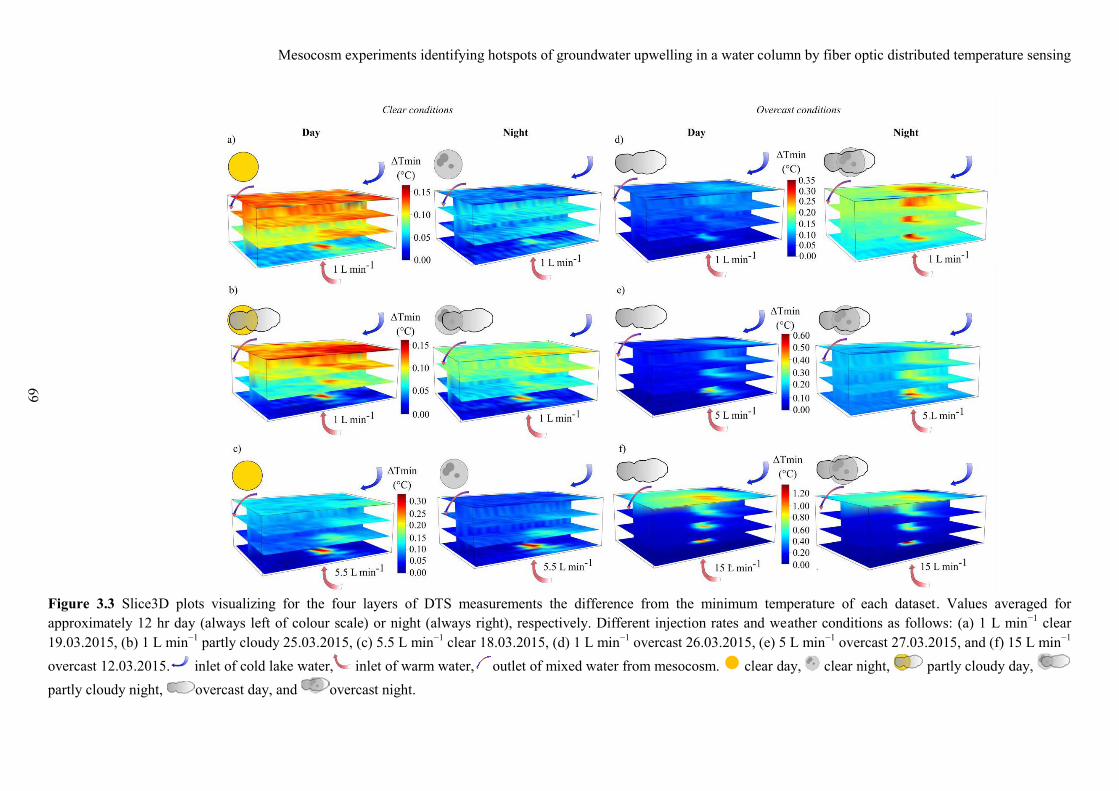
Mesocosm experiments identifying hotspots of groundwater upwelling in a water column by fiber optic distributed temperature sensing
69
Figure 3.3 Slice3D plots visualizing for the four layers of DTS measurements the difference from the minimum temperature of each dataset. Values averaged for
approximately 12 hr day (always left of colour scale) or night (always right), respectively. Different injection rates and weather conditions as follows: (a) 1 L min−1 clear
19.03.2015, (b) 1 L min−1 partly cloudy 25.03.2015, (c) 5.5 L min−1 clear 18.03.2015, (d) 1 L min−1 overcast 26.03.2015, (e) 5 L min−1 overcast 27.03.2015, and (f) 15 L min−1
overcast 12.03.2015. inlet of cold lake water, inlet of warm water, outlet of mixed water from mesocosm. clear day, clear night, partly cloudy day,
partly cloudy night, overcast day, and overcast night.

70
3.3.2 Quantitative analysis of spatial temperature patterns
Horizontal spatial temperature patterns: Spatial autocorrelation within layers: Moran’s I
scatter plots and LISA maps
All datasets show significant spatial autocorrelation between data points within each layer
with p values less than 2.2 e−16
, except the dataset of Layer 3 at an injection rate of 1 L min−1
at night under clear sky conditions where the p value is 1.18 e−06
. As an example, Figure 3.4
compares the Moran's I scatter plots and LISA maps during daytime for 1 L min−1
clear sky
and 15 L min−1
overcast sky conditions. When injecting 1 L min−1
with clear sky conditions,
despite the significant spatial autocorrelation, the temperature data values are more dispersed
over the four quadrants. Figure 3.4a indicates potential influential observations in Layers 1
and 2, mainly located in the quadrant “high-high,” identifying a positive spatial
autocorrelation between observation points surrounding those data values. However, in
Layers 3 and 4 (Figure 3.4a), the distribution of potential influential observations over the
four quadrants is more dispersed, not showing a clear clustering of points on “high-high” and
“low-low” quadrants (in red and yellow in LISA maps, Figure 3.4c).
On the contrary, temperatures observed for the 15 L min−1
injection rate show stronger spatial
autocorrelation with most of the data points in high-high and low-low quadrants indicating a
positive spatial autocorrelation (Figure 3.4b and 3.4d). Thus, the spatial autocorrelation over
the four layers is stronger than in the dataset of 1 L min−1
and clear sky condition.
Furthermore, LISA maps (Figure 3.4d) show a clear clustering of the highly spatially
autocorrelated values.
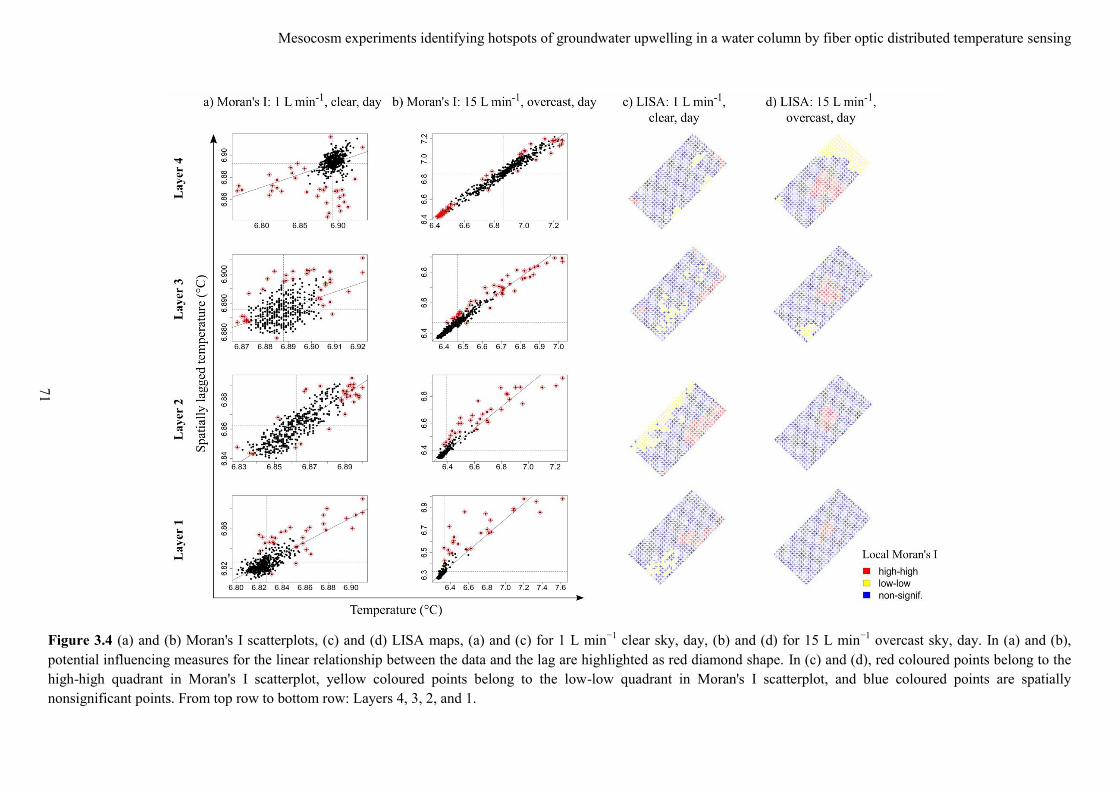
Mesocosm experiments identifying hotspots of groundwater upwelling in a water column by fiber optic distributed temperature sensing
71
Figure 3.4 (a) and (b) Moran's I scatterplots, (c) and (d) LISA maps, (a) and (c) for 1 L min−1 clear sky, day, (b) and (d) for 15 L min−1 overcast sky, day. In (a) and (b),
potential influencing measures for the linear relationship between the data and the lag are highlighted as red diamond shape. In (c) and (d), red coloured points belong to the
high-high quadrant in Moran's I scatterplot, yellow coloured points belong to the low-low quadrant in Moran's I scatterplot, and blue coloured points are spatially
nonsignificant points. From top row to bottom row: Layers 4, 3, 2, and 1.
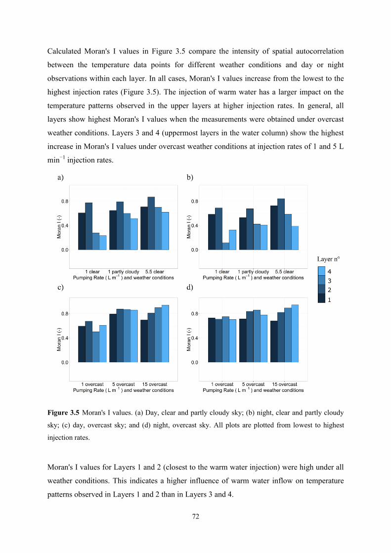
72
Calculated Moran's I values in Figure 3.5 compare the intensity of spatial autocorrelation
between the temperature data points for different weather conditions and day or night
observations within each layer. In all cases, Moran's I values increase from the lowest to the
highest injection rates (Figure 3.5). The injection of warm water has a larger impact on the
temperature patterns observed in the upper layers at higher injection rates. In general, all
layers show highest Moran's I values when the measurements were obtained under overcast
weather conditions. Layers 3 and 4 (uppermost layers in the water column) show the highest
increase in Moran's I values under overcast weather conditions at injection rates of 1 and 5 L
min−1
injection rates.
Figure 3.5 Moran's I values. (a) Day, clear and partly cloudy sky; (b) night, clear and partly cloudy
sky; (c) day, overcast sky; and (d) night, overcast sky. All plots are plotted from lowest to highest
injection rates.
Moran's I values for Layers 1 and 2 (closest to the warm water injection) were high under all
weather conditions. This indicates a higher influence of warm water inflow on temperature
patterns observed in Layers 1 and 2 than in Layers 3 and 4.

Mesocosm experiments identifying hotspots of groundwater upwelling in a water column by fiber
optic distributed temperature sensing
73
Under clear sky weather conditions, Moran's I values for Layers 1 and 2 are similar or
decrease slightly during night measurements. For Layers 3 and 4, Moran's I values during
night are lower than Moran's I values during day measurements.
Under overcast weather conditions, Moran's I values within Layers 1, 2, 3, and 4 for 1 L
min−1
injection rate increase during night measurements. For an injection rate of 5 L min−1
,
Moran's I values for Layers 1 and 4 are lower during night than during day measurements.
Finally, Moran's I values for 15 L min−1
injection rate are very similar during day and night
measurements.
In summary, significant spatial autocorrelations within each layer have been identified in all
datasets. However, calculated Moran's I values vary depending on the injection rate of warm
water, weather conditions, and the diurnal cycle (see Figure 3.5). This indicates that the
strength of the spatial pattern within each layer also varies depending on the injection rates
applied, the weather conditions, and the diurnal cycle.
Vertical spatial temperature patterns: Spatial correlation between layers
Spatial correlation between neighboring layers
At high injection rates, the largest correlations between neighbouring layers occurred (Table
S1). At lower injection rates, the correlation was usually much smaller and the largest
correlation generally occurred between neighbouring layers. There are three exceptions where
the largest correlations occurred between nonneighbouring layers: dataset 1 L min−1
, clear,
daytime and 1 L min−1
, partly cloudy, day and night-time. The reason might be that the extent
of the spatial warm water pattern in Layers 1 and 3 is more similar than the observed pattern
in Layer 2 (See Figures 3.4c and S1).
Measurements under clear sky conditions with an injection rate of 1 L min−1
showed a
downward trend (from Layer 1 to 4) on spatial correlation coefficients calculated between
neighbouring layers (1&2, 2&3, 3&4). When weather conditions were “partly cloudy” for 1 L
min−1
, spatial correlation coefficients calculated between neighbouring layers showed an
upward trend from Layer 1 to 3 (1&2 and 2&3) and the lowest value between the two
uppermost layers (3&4). Finally, when weather conditions were overcast and injecting 1 L
min−1
, it is possible to see that there was an upward trend (from Layer 1 to 4) on spatial
correlation coefficients calculated between neighbouring layers (1&2, 2&3, 3&4), for
example, from 0.415 to 0.815 during day.

74
The same upward trend was observed for an injection rate of 5.5 L min−1
with clear sky
conditions for spatial correlation coefficients calculated between neighbouring layers: from
0.516 to 0.685. At injection rate of 5 L min−1
with overcast conditions, spatial correlation
coefficients between neighbouring layers keep increasing, for example, from 0.795 to 0.933
day.
On the contrary, when injecting 15 L min−1
, calculated spatial correlation coefficients
between neighbouring layers only increase for layers 1&2 and 2&3 from 0.846 to 0.888.
Spatial correlation coefficients for 3&4 layers decrease to 0.450.
Spatial correlation between nonneighbouring layers
Highest spatial correlations calculated between nonneighbouring layers (1&3, 1&4, and 2&4)
were found for 1 L min−1
under overcast conditions during night (0.681, 0.572, and 0.663,
respectively) and for 5 L min−1
under overcast conditions during day (0.608, 0.546, and
0.791, respectively).
Spatial correlation coefficients between Layers 1&3 generally increase from 1 to 15 L min−1
under overcast conditions. Spatial correlation coefficients between layers 1&4 and 2&4
generally increase from 1 to 5 L min−1
and considerably decrease at 15 L min−1
. These
observations agree with the change on the spatial pattern observed in Figure 3.3f, compared
with the spatial patterns observed in Figures 3.3d and 3.3e. In Figure 3.3f, injected warm
water flows straight up across Layers 1, 2, and 3. In Layer 4, injected warm water spreads all
over the water surface. Low spatial correlation coefficients for 15 L min−1
between Layers
2&4 and 1&4 indicate differences of spatial patterns observed between Layers 1&4 and 2&4
in Figure 3.3f.
Figure 3.6 presents calculated spatial correlation coefficients for different (clear sky, partly
cloudy, and overcast) conditions for both day and night measurements independently.
Spatial correlation coefficients calculated between 1&2, 1&3, and 2&3 are higher during
night than during day. However, spatial correlation coefficients calculated for 1&4, 2&4, and
3&4 showed different results. For clear sky conditions, calculated spatial correlation
coefficients during night time are lower than calculated spatial correlation coefficients for the
same injection rates during day. In contrast, calculated spatial correlation coefficients for
overcast weather conditions are slightly higher during night than during day within the same
injection rates, for both 1 and 15 L min−1
. In contrast, for 5 L min−1
under overcast
conditions, spatial correlation coefficients are slightly lower during night than during day.

Mesocosm experiments identifying hotspots of groundwater upwelling in a water column by fiber
optic distributed temperature sensing
75
Figure 3.6 Spatial correlation coefficients for (a) day, clear sky and partly cloudy conditions; (b)
night and clear sky, partly cloudy conditions; (c) day and overcast conditions; (d) night and overcast
conditions.
Three main findings can be listed from the calculation of spatial correlation coefficients
between layers:
In general, overcast weather conditions result in higher spatial correlation coefficients
between neighbouring layers and nonneighbouring layers.
At 15 L min−1
, the uppermost layer (Layer 4) is spatially less correlated with the
underlying layers than at 1 and 5 L min−1
under overcast conditions. These
observations agree with the change on the spatial pattern observed in Figure 3.3f in
comparison with the spatial patterns observed in Figure 3.3d,e.
The diurnal cycle has an effect on spatial correlation coefficients calculated between
layers. Layers within the water column show higher spatial correlation coefficients
between them during night than during day for the same injection rates no matter of
the weather conditions. However, for the uppermost layer (Layer 4) at the water

76
surface–atmosphere interface, spatial correlation coefficients are lower for clear nights
and generally similar or slightly higher for overcast nights.
3.3.3 Net heat fluxes across the water surface, advective heat fluxes and
internal energy change
The effects of different weather conditions, different injection rates, and the diurnal cycle on
the energy balance of the water column were quantified. This was done by quantifying the net
heat fluxes across the water surface (G in W m−2
) as well as the energy change due to
advective transport by the water inlet from the lake, the warm water inlet at the bottom of the
mesocosm and the water outlet from the mesocosm (Eadv in MJ). Their sum results in the
change of internal energy in the mesocosm (ΔE in MJ).
Net heat fluxes across the water surface (G)
Net heat fluxes across the water surface (G) during day and night are composed of net
radiation (Rn), latent heat fluxes (phase transformation, λE), and sensible heat fluxes (H) with
Rn being the most important of the three (see Figure 3.7a,c,e,g,i,k,m). This indicates that the
system gains and loses energy mainly by Rn.
Net radiation (Rn) is composed of net shortwave radiation (Rns) and net longwave radiation
(Rnl). The net shortwave radiation (Rns) is considered a heating term (during daytime) and the
net longwave radiation (Rnl) is considered a cooling term (during day and night; Betts, 2015).
Therefore, during daytime, calculated Rn values are higher than during night for both clear
and overcast weather conditions (Figure 3.7a, c,e,g,i,k,m). This is because during daytime,
the surface cooling due to Rnl is partly compensated by Rns (Betts, 2003, 2015; Betts,
Desjardins, & Worth, 2013). In addition, during night, there is no shortwave radiation coming
from the sun and the cooling term, Rnl, will be the main component of the Rn.
In general, Rn values during daytime are lower under overcast weather conditions than under
clear sky conditions (Figure 3.7a,c,e,g,i, k,m). During night, Rn values are less negative under
overcast conditions than under clear sky conditions (Figure 3.7a,c,e,g,i,k,m). These results
are related to the important effect that clouds have on the net radiation balance (Rn; Betts,
2015). On the one hand, during daytime, incident downward shortwave radiation at the water
surface is lower under overcast weather conditions than under clear sky conditions. On the
other hand, during day and night, surface cooling to space due to Rnl is lower under overcast
weather conditions than under clear sky conditions (Betts, 2003, 2015; Betts et al., 2013).
The smallest net heat fluxes across the water surface (G) occur under overcast conditions (see
Figure 3.7a,g,k,m).
Mesocosm experiments identifying hotspots of groundwater upwelling in a water column by fiber
optic distributed temperature sensing
77
Energy transferred across the interface (EG) and advected energy by inflows and outflows
(Eadv)
For all datasets, during daytime measurements, the system gains energy mainly by EG and
during night time measurements by Eadv (Figure 3.7b,d,f, h,j,l). Only, for 15 L min−1
overcast
weather conditions dataset, the system mainly gains energy by Eadv during day and night due
to the high amounts of injected warm water (Figure 3.7n). This means that the energy gains in
the mesocosm during day are dominated by the net heat fluxes across the water surface (G)
and the energy losses in the mesocosm are dominated by the energy transported by advection
into and out of the mesocosm. On the contrary, the energy gains in the mesososm during
night are dominated by the imported energy of the injected warm water (Eadv) and the energy
losses in the mesocosm are dominated by the net heat fluxes across the water surface (G).
Internal energy changes in the mesocosm (∆E)
ΔE changes over time are clearly affected by the diurnal cycle (see Figure 3.8). ΔE decreases
during the day; it reaches a minimum during night and increases again in the early morning.
However, the intensity of changes of ΔE over time varies depending on weather conditions
and injection rate.
ΔE changes over time are lowest under overcast weather conditions for all different injection
rates. The dataset with an injection rate of 1 L min−1
shows the lowest ΔE changes over time,
and 15 L min−1
shows the highest ΔE changes over time.
High changes on ΔE over time are observed when injecting 1 L min−1
under clear sky
conditions. For partly cloudy conditions, keeping the same injection rate, the maximum loss
of energy over time is smaller than under clear sky weather conditions. However, the slope of
ΔE in Figure 3.8 for 1 L min−1
partly cloudy is higher than that of the 1 L min−1
clear sky
during day; this indicates that the rate of energy loss is greater. On increasing the injection
rate to 5.5 L min−1
under clear sky, maximum energy loss in the system is almost similar to
the maximum energy loss when injecting 1 L min−1
under clear sky. However, change of ΔE
over time is greater when injecting 5.5 L min−1
under clear sky than when injecting 1 L min−1
under clear sky.

78
Figure 3.7 Calculated heat fluxes
across the water surface (G), net
radiation (Rn) evaporative heat flux
(λE), and sensible heat flux (H) for (a)
control dataset with 0 L min−1
injection rate, overcast, (c) 1 L min−1
clear, (e) 1 L min−1
partly cloudy, (g)
1 L min−1
overcast, (i) 5.5 L min−1
clear, (k) 5 L min−1
overcast, and (m)
15 L min−1
overcast and calculated
ΔE, EG and Eadv for (b) control
experiment overcast (d) 1 L min−1
clear, (f) 1 L min−1
partly cloudy, (h) 1
L min−1
overcast, (j) 5.5 L min−1
clear,
(l) 5 L min−1
overcast, and (n) 15 L
min−1
overcast.
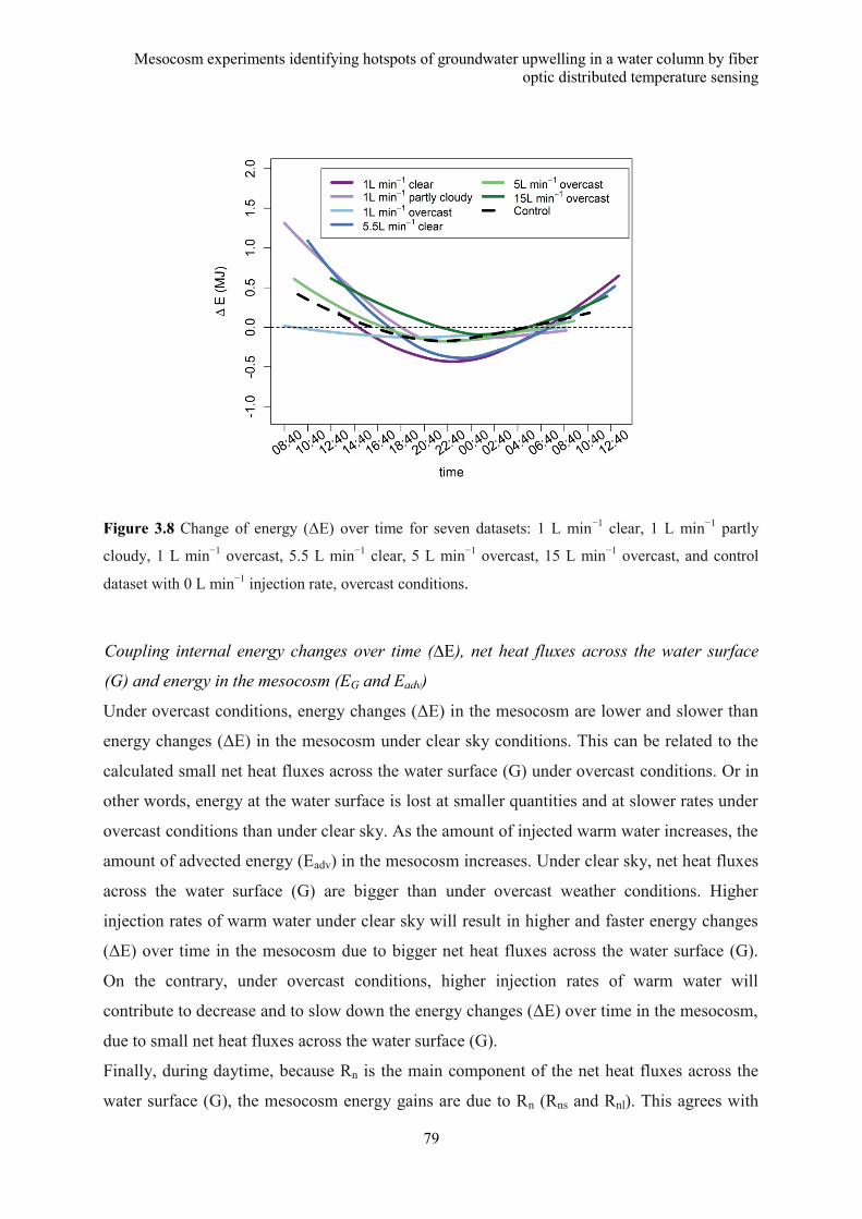
Mesocosm experiments identifying hotspots of groundwater upwelling in a water column by fiber
optic distributed temperature sensing
79
Figure 3.8 Change of energy (ΔE) over time for seven datasets: 1 L min−1
clear, 1 L min−1
partly
cloudy, 1 L min−1
overcast, 5.5 L min−1
clear, 5 L min−1
overcast, 15 L min−1
overcast, and control
dataset with 0 L min−1
injection rate, overcast conditions.
Coupling internal energy changes over time (∆E), net heat fluxes across the water surface
(G) and energy in the mesocosm (EG and Eadv)
Under overcast conditions, energy changes (ΔE) in the mesocosm are lower and slower than
energy changes (ΔE) in the mesocosm under clear sky conditions. This can be related to the
calculated small net heat fluxes across the water surface (G) under overcast conditions. Or in
other words, energy at the water surface is lost at smaller quantities and at slower rates under
overcast conditions than under clear sky. As the amount of injected warm water increases, the
amount of advected energy (Eadv) in the mesocosm increases. Under clear sky, net heat fluxes
across the water surface (G) are bigger than under overcast weather conditions. Higher
injection rates of warm water under clear sky will result in higher and faster energy changes
(ΔE) over time in the mesocosm due to bigger net heat fluxes across the water surface (G).
On the contrary, under overcast conditions, higher injection rates of warm water will
contribute to decrease and to slow down the energy changes (ΔE) over time in the mesocosm,
due to small net heat fluxes across the water surface (G).
Finally, during daytime, because Rn is the main component of the net heat fluxes across the
water surface (G), the mesocosm energy gains are due to Rn (Rns and Rnl). This agrees with
80
EG being the main driver of gains of energy in the mesocosm during daytime. If the
mesocosm is subject to strong gains of energy due to Rn during day (for instance under clear
sky), it means that energy gains by Rns will prevail over energy losses by Rnl. During night,
the main losses of energy in the mesocosm are driven by Rn (only Rnl). This agrees with EG
being the main driver of losses of energy in the mesocosm during night.
Observed spatial patterns of injected warm water in the mesocosm, net heat fluxes across the
water surface (G) and energy changes over time (∆E)
Spatial patterns of injected warm water across the water column and at the water surface
observed in Figure 3.3d–f can be related to small and slow energy changes (ΔE) over time,
due to small net heat fluxes across the water surface (G) under overcast weather conditions
during day and night. During daytime, the heat signal of the injected warm water will prevail
across the water column and at the water surface due to: 1) less absorbed shortwave radiation
at the water surface of the mesocosm (Rns) and 2) less water surface cooling in the mesocosm
due to Rnl. During night-time, the heat signal of the injected warm water will prevail across
the water column and at the water surface due to: 1) less water surface cooling in the
mesocosm due to Rnl and 2) energy gains in the mesocosm due to injected warm water.
Finally, spatial patterns of injected warm water, across the water column and at the water
surface, observed in Figure 3.3a–c can be related to high and fast energy changes (ΔE) over
time in the mesocosm, due to stronger net heat fluxes across the water surface (G) under clear
sky during day and night, than under overcast conditions. In general, during daytime, the heat
signal of the injected warm water is not detectable at the water surface, mainly due to high
amount of absorbed shortwave radiation at the water surface (Rns) during clear sky and to a
less extent, due to water surface cooling in the mesocosm by Rnl. During night, the heat signal
of the injected warm water is not detectable at the water surface due to strong cooling of the
water surface in the mesocosm by Rnl.
3.4 Discussion
Detectability of upwelling signals
One basic question of the present study is if and under which circumstances the lake-internal
upwelling pattern due to simulated GW discharge can be detected in the water column and at
the water surface. For that purpose, temperature signals due to the positive buoyancy of
relatively warm water need to be separated from other temperature fluctuations. In the context
of the present study, strong spatial autocorrelations within layers and strong spatial
Mesocosm experiments identifying hotspots of groundwater upwelling in a water column by fiber
optic distributed temperature sensing
81
correlations between layers are interpreted as “real” temperature signal related to the positive
buoyancy of relatively warm water, instead of to other temperature fluctuations. Moran's I
and LISA maps (indicators for horizontal spatial patterns within layers) confirmed the spatial
patterns visually observed in Figure 3.3. The strength of spatial autocorrelation within layers
(horizontal spatial patterns) increased under overcast conditions, at higher injection rates and
during night-time. Calculated spatial correlation coefficients between layers (vertical spatial
patterns) also increased under overcast weather conditions, higher injection rates, and during
night-time measurements. At 15 L min−1
injection rate, spatial correlation coefficients
between Layer 4 (the uppermost layer) and the other layers decreased due to a change of the
general shape of the upwelling flume (Figure 3.3f and Figure 3.9, a.6 and b.6). Due to the
intense injection rate, the warm water signal travels straight upwards, and once it reaches the
water surface, it spreads horizontally at the water surface.
Relevance of diurnal cycle and cloud cover on signal detectability
Under overcast conditions, calculated slow energy changes (ΔE) over time and low net heat
fluxes across the water surface (G) seem to be related to the spatial patterns in Figure 3.3d–f
and the results obtained with the Moran's I coefficient, LISA maps, and the spatial correlation
coefficients. Slow changes of energy (ΔE) over time and low net heat fluxes across the water
surface (G) indicate that the mesocosm is able to sustain internal energy for longer time
periods than under clear sky conditions. This means that the heat signal related to warm water
injection is not lost. On the contrary, in datasets under clear and partly cloudy conditions,
higher energy changes (ΔE) over time and higher net heat fluxes across the water surface (G)
were calculated. In other words, the mesocosm loses internal energy faster over time, and
consequently, the heat signal related to warm water injection is lost faster over time under
clear sky conditions.
The amount of energy in a water body (for instance, a lake) is controlled by the inflows and
outflows of water into and out of the water body and by heat fluxes across the water surface,
among others (Henderson-Sellers, 1986). The net heat fluxes across the water surface (G) are
composed of net shortwave radiation (Rns), net longwave radiation (Rnl) and nonradiative
fluxes (sensible heat [H] and latent heat [λE]; Henderson-Sellers, 1986; McAlister &
McLeish, 1969). The main component for calculated net heat fluxes across the water surface
(G) is the net radiation (Rn), which is the sum of net shortwave radiation (Rns) and net
longwave radiation (Rnl). The net radiation balance is driven by the diurnal cycle of the
incident shortwave radiation (Betts, 2015). This means that the solar warming during daytime
82
and the longwave cooling during night-time drive the diurnal cycles of air temperature and
water surface temperature (Betts, 2015; Vercauteren et al., 2011) and, thus, impact on the
detectability of the injected warm water temperature signal in the mesocosm. Furthermore,
cloud cover is also a relevant regulator of the diurnal cycle of the net radiation balance (Rn;
Betts, 2003, 2015; Betts et al., 2013; Dai & Trenberth, 1999). Clouds decrease the incident
shortwave radiation at the water surface and decrease the net surface cooling at the water
surface because there is less Rnl. Therefore, the detectability of the injected warm water
temperature signal in the mesocosm is decisively controlled by the diurnal cycle of the net
radiation balance (Rn) and the cloud cover. In order to illustrate the relevance of the diurnal
cycle (day vs. night) of the net radiation balance (Rn = Rns + Rnl) and cloud cover on the
observed spatial patterns of the heat signal related to warm water injection and based on the
results presented in this paper, a conceptual model for the spatial patterns observed under
different weather conditions (clear, partly cloudy, and overcast), injection rates, and diurnal
cycles (day vs. night) is suggested in Figure 3.9. It illustrates the relevance of the net heat
fluxes across the water surface (G) by the strength of net short wave (Rns) and net long wave
(Rnl) radiation (conceptualized by size of arrow: big: high values, small: low values) for
different injection rates, different weather conditions (clear, partly cloudy, and overcast), and
diurnal cycles (day vs. night). During day, the main gains or losses of heat at the mesocosm's
water surface are due to the Rn (=Rns + Rnl). During clear sky conditions during daytime, due
to the higher solar warming (Rns) at the water surface than during overcast weather
conditions, the water surface is heated up. In consequence, the heat signal of the injected
warm water at the water surface is mixed with the heated water surface due to solar warming.
On the contrary, during overcast weather conditions during daytime, calculated Rn (see Figure
3.7) and solar warming due to Rns are lower. In consequence, the heat signal of the injected
warm water can be detected at the water surface (see Figure 3.9a). During night, because
there is no Rns, the main gains or losses of heat at the mesocosm's water surface are due to
Rnl. Both, during night and day, the degree of heat losses from the water surface depends on
the presence of clouds at the sky (see Figure 3.9b). During clear sky conditions, the strength
of Rnl is higher than under overcast weather conditions. In consequence, during clear sky
conditions at night, the mesocosm loses higher amounts of energy across the water surface–
atmosphere interface than during overcast conditions. The heat signal of the injected warm
water at the water surface is lost faster during clear sky conditions than during overcast
conditions at night (Figure 3.9b).
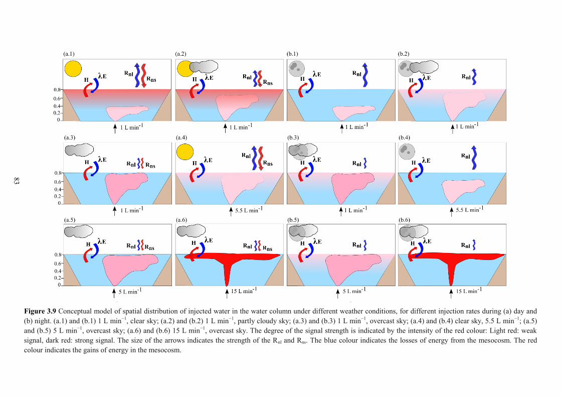
83
Figure 3.9 Conceptual model of spatial distribution of injected water in the water column under different weather conditions, for different injection rates during (a) day and
(b) night. (a.1) and (b.1) 1 L min−1, clear sky; (a.2) and (b.2) 1 L min−1, partly cloudy sky; (a.3) and (b.3) 1 L min−1, overcast sky; (a.4) and (b.4) clear sky, 5.5 L min−1; (a.5)
and (b.5) 5 L min−1, overcast sky; (a.6) and (b.6) 15 L min−1, overcast sky. The degree of the signal strength is indicated by the intensity of the red colour: Light red: weak
signal, dark red: strong signal. The size of the arrows indicates the strength of the Rnl and Rns. The blue colour indicates the losses of energy from the mesocosm. The red
colour indicates the gains of energy in the mesocosm.
84
Application of FO-DTS for detection of LGD upwelling
FO-DTS has been used to detect GW discharge at the sediment–water interface in lakes
(Blume et al., 2013; Liu et al., 2015; Tristram et al., 2015) and streams (Hare et al., 2015;
Krause et al., 2012; Lowry et al., 2007). However, it had not yet been determined how the
temperature signal propagates from the sediment–water interface through the water column up
to the water surface–atmosphere interface and how the signal is affected by environmental
parameters such as weather conditions (clear vs. overcast) and the diurnal cycle of net
radiation. In Hare et al. (2015), FO-DTS measurements were compared with thermal infrared
(TIR) measurements, which allowed the comparison of heat signals detected at the stream bed
and at the water surface. Winter conditions were proven to be the best season to conduct these
kinds of measurements. However, the characterization of weather and diurnal conditions that
might have affected the upwelling patterns of the GW heat signal across the water column was
not addressed until the present study. For instance, Liu et al. (2015) conducted an experiment
on the lake bed that took into account environmental factors to determine the best time to
detect GW discharge areas with FO-DTS. Liu et al. (2015) worked in a lake that was
relatively shallow, which reduced the effect of vertical stratification on the lakebed
temperatures during the FO-DTS measurements. Nevertheless, the FO-DTS experiment
conducted did not include multilevel temperature measurements or a detailed characterization
of the influence of weather conditions and the diurnal cycle of net radiation on the detection
of GW discharge across the water column.
The knowledge gap on upwelling GW heat signals monitored with FO-DTS across the water
column may have led to misinterpretations. This is because the temperature within the water
column may be affected by several external parameters. Therefore, timing and conditions
when measuring warm upwelling fluxes with FO-DTS are of great relevance for the
interpretation of the results. For instance, it is crucial to be aware of the vertical positioning of
the cable because variations of the vertical positioning of the cable on the sediment or within
the water column may lead to misinterpretations of the patterns observed. Variable external
conditions have to be taken into account for correct interpretation that might present a real
difficulty for any quantitative assessment. Therefore, it is essential to determine those
parameters that may influence the temperature such as solar radiation and to make sure that
the temperature variations of the lake as detected by the FO-DTS are mainly caused by GW
discharge (Liu et al., 2015) as presented in this paper.
Mesocosm experiments identifying hotspots of groundwater upwelling in a water column by fiber
optic distributed temperature sensing
85
Possible system interferences and uncertainties of the study
Effect of wind and possible consequences
Wind is an important factor affecting lake SW temperatures and lake internal mixing (Pöschke
et al., 2015). Wind promotes movement and mixing of SW bodies. The SW can be dragged by
the wind from one shore of a lake to the other shore inducing downwelling of water in the
water body on one side of the lake and at the same time water movement from the bottom of
the lake upwards to the lake surface (mixing). This process, relevant in lake settings, is
probably irrelevant in the small experimental mesocosm used in the present study. From the
slice3D plots in Figure 3.3, there is no indication for a wind-induced circulation or mixing.
Wind speeds during the experiments were generally low (ranging from 0.0045 to 2.1789 m
s−1
). Steep bank slopes reaching a height of 1 m above the water surface prohibited wind
impacts on the water surface. Furthermore, due to the small size of the mesocosm, the wind
fetch is short and a potential wind impact on the water surface is irrelevant. However, when
transferring the results of the mesocosm experiment to a real lake setting, possible wind
impacts should be taken into account.
Thickness of water column in the present study
In the present study, the thickness of the water column is 0.82 m. The obtained conclusions
could be directly transferred to shallow lakes not deeper than 1 m, shore areas of lakes not
deeper than 1 m, and probably to shallow lakes with slightly larger depth. Because there is no
thermal stratification within the water column of the mesocosm, the obtained results of the
present study can only be transferred to cases where there is no thermal stratification.
Possible effects of electrical conductivity of groundwater
The upwelling of the water injected at the mesocosm's bottom is driven by density differences
of the injected water and the water in the mesocosm. The density differences are caused by
different temperatures and different ion compositions of the two waters. The water in the
mesocosm is a mixture of lake water and water previously injected at the mesocosm's bottom.
Due to differing injection rates during the different experiments, there is no constant
relationship between the relatively large inflow from the lake (33 L min−1
) and the relatively
small inflow from the injection at the mesocosm's bottom (0 to 15 L min−1
). For simplicity,
we assume that the mesocosm water composition is basically identical to the lake water
composition. On the basis of measurements of the ion composition of both water bodies, we
86
ended up with total dissolved solid concentrations of 489 mg L−1
for the lake and 429 mg L−1
for the injected water, that is, there is a density difference of 60 mg L−1
between the two
waters. Based on a mean mesocosm temperature of 4.7 °C, the density of the water in the
mesocosm is 0.999946 kg L−1
, and based on a mean temperature of 15 °C of the injected
water, the density is 0.999114 kg L−1
, that is, there is a density difference of 832 mg L−1
between the two waters. Basically, the density difference due to the different ion composition
of the two different waters, strengthen the temperature induced density difference. The
combined effect of ion composition and temperature on the density difference between the
two waters is 880 mg L−1
(calculation according to Dietz, Lessmann, & Boehrer, 2012) or 921
mg L−1
(calculation according to Boehrer & Herzsprung, 2010).
Therefore, the injected warm water should immediately rise upwards through the surrounding
denser lake water via buoyancy. During the short ascent, some mixing might have occurred
and the contact with surrounding water resulted in some cooling of the injected warm water.
Nevertheless, only in experiments during overcast conditions (Figure 3.3d–f), the injected
warm water was still warmer than the rest of the water in the mesocosm when it reached the
water surface and thus, floated on the top of the water body. From there, the warmer less
dense water gradually spread as a plume on the water surface.
Low wind speeds, shallow water conditions, and density differences between simulated GW
and SW might favour the upwelling of simulated GW discharge on the SW. However, in the
present study, the main parameters controlling the detection of simulated GW on the water
surface seem to be the net radiation balance (Rn) and the cloud cover during day and night-
time measurements. Because the experiments have been carried out under specific conditions,
the previous statements are only true in lake areas where the same conditions apply as in the
mesocosm experiment during winter conditions.
This study is a first attempt to simulate thermal patterns of discrete LGD in shallow lakes or
close to lake shores. The mesocosm experiment and simulation of GW discharge is the first
step in order to identify the main controlling parameters that favour detection of hotspots of
LGD on the lake surface (mesocosm surface in this case). We have decreased the amount of
variables that impact LGD by simulating discrete GW discharge in a mesocosm. The
mesocosm where the simulation has been performed intends to represent a small shallow area
of a lake where GW exfiltration by LGD occurs. Thus, not all the influencing factors such as
wind, waves, and vegetation that could be present under natural conditions have been
considered. However, GW discharge that is warmer than SW has been little studied relative to
Mesocosm experiments identifying hotspots of groundwater upwelling in a water column by fiber
optic distributed temperature sensing
87
discharge of cold GW to warmer SW. Thus, by conducting studies during colder times of the
year, scientist can make use of the conclusions presented here.
3.5 Conclusion
The present study demonstrates that during winter conditions, the positive buoyancy of
relatively warm water imported by simulated LGD into shallow water bodies (mesocosm used
as model system) allows detection of LGD at the lake's water surface–atmosphere interface by
FO-DTS. FO-DTS technology offers fine scale measurements with high temporal resolution
and allows the observation of induced lake-internal upwelling caused by simulated LGD in a
three-dimensional perspective. In this manner, different lake internal upwelling patterns have
been described from the sediment–water interface through the water column to the water
surface–atmosphere interface caused by the injection of warm water at different rates,
different weather conditions, and during the diurnal cycle. Simulated GW signals at the water
surface were identified at all applied injection rates, from lowest 1 L min−1
to highest 15 L
min−1
. However, detection of simulated LGD at the water surface–atmosphere interface was
mainly determined by the diurnal cycle of the net radiation balance (Rn) and the cloud cover.
Based on the results presented in this paper, overcast weather conditions and night-time
measurements are recommended for tracing discrete warm water upwelling fluxes across the
water column and at the water surface.
Acknowledgments
Funding: This work was supported by the European Union’s Seventh Framework programme
for research, technological development and demonstration [grant number 60715]:
Ecohydrological Interfaces as Critical Hotspots for Transformations of Ecosystem Exchange
Fluxes (INTERFACES).
Special thanks to Franziskca Pöschke, Karin Meinikmann, Hauke Dämpfling and Anne
Mehrtens.
Supporting information
Appendix S1: Quantification of interfacialne heat transfer and net-advective heat flux
Appendix S2: Nomenclature
Figure S1: Comparison of LISA maps and spatial correlation coefficients between layer 1
and 2 and layer 1 and 3 for datasets: a) 1 L min-1
clear conditions, daytime, b) 1 L min-1
partly

88
cloudy conditions, daytime and c) 1 L min-1
partly cloudy conditions, night-time. From top
row to bottom row: layer 4, layer 3, layer 2 and layer 1.
Table S1. Spatial correlation coefficients between layers.
Mesocosm experiments identifying hotspots of groundwater upwelling in a water column by fiber
optic distributed temperature sensing
89
References
Anselin L. 1995. Local Indicators of Spatial Association-LISA. Geographical Analysis 27 (2):
93–115 DOI: 10.1111/j.1538-4632.1995.tb00338.x
Anselin L. 1996. The Moran scatterplot as an ESDA tool to assess local instability in spatial
association. In Spatial Analytical Perspectives on GIS111–125.
Apperl B, Pressl A, Schulz K. 2017. Feasibility of Locating Leakages in Sewage Pressure
Pipes Using the Distributed Temperature Sensing Technology. Water, Air, and Soil
Pollution 228 (2) DOI: 10.1007/s11270-017-3250-7
Baker BH, Martinovic-Weigelt D, Ferrey M, Barber LB, Writer JH, Rosenberry DO, Kiesling
RL, Lundy JR, Schoenfuss HL. 2014. Identifying non-point sources of endocrine active
compounds and their biological impacts in freshwater lakes. Archives of environmental
contamination and toxicology 67 (3): 374–388 DOI: 10.1007/s00244-014-0052-4
Betts AK. 2003. The diurnal cycle over land. In Forests at the Land-Atmosphere Interface,
Mencuccini M, , Grace J, , Moncrieff J, , McNaughton K (eds).CABI Publishing,
Wallingford, Oxon OX10 8DE, UK; 73–93.
Betts AK. 2015. Diurnal Cycle. In Encyclopedia of Atmospheric Sciences, Pyle J, , Fuqing Z
(eds).Texas A&M University, College Station, TX, USA; 319–323. DOI: 10.1016/B978-
0-12-382225-3.00135-3
Betts AK, Desjardins R, Worth D. 2013. Cloud radiative forcing of the diurnal cycle climate
of the Canadian Prairies. Journal of Geophysical Research 118 (June): 8935–8953 DOI:
10.1002/jgrd.50593
Bivand RS, Pebesma E, Gómez-Rubio V. 2013. Applied Spatial Data Analysis with R.
Springer-Verlag New York. DOI: 10.1007/978-1-4614-7618-4
Blume T, Krause S, Meinikmann K, Lewandowski J. 2013. Upscaling lacustrine groundwater
discharge rates by fiber-optic distributed temperature sensing. Water Resources Research
49 (October 2012): 7929–7944 DOI: 10.1002/2012WR013215
Boehrer B, Herzsprung P. 2010. Calculating density of water in geochemical lake
stratification models. Limnology and oceanography, methods (1): 567–574 DOI:
10.4319/lom.2010.8.567
Brabrand Å, Koestler AG, Borgstrøm R. 2002. Lake spawning of brown trout related to
groundwater influx. Journal of Fish Biology 60 (3): 751–763 DOI:
10.1006/jfbi.2002.1901

90
Brunke M, Gonser T. 1997. The ecological significance of exchange processes between rivers
and groundwater. Freshwater Biology 37: 1–33 DOI: 10.1046/j.1365-2427.1997.00143.x
Cardenas MB, Lagmay AMF, Andrews BJ, Rodolfo RS, Cabria HB, Zamora PB, Lapus MR.
2012. Terrestrial smokers: Thermal springs due to hydrothermal convection of
groundwater connected to surface water. Geophysical Research Letters 39 (2): 1–6 DOI:
10.1029/2011GL050475
Curry RA, Noakes DLG. 1995. Groundwater and the selection of spawning sites by brook
trout ( Salvelinus fontinalis ). Canadian Journal of Fisheries and Aquatic Sciences 52 (8)
DOI: 10.1139/f95-765
Dai A, Trenberth KE. 1999. Effects of Clouds , Soil Moisture , Precipitation , and Water
Vapor on Diurnal Temperature Range. Journal of Climate 12: 2451–2473
Dietz S, Lessmann D, Boehrer B. 2012. Contribution of Solutes to Density Stratification in a
Meromictic Lake (Waldsee/Germany). Mine Water and the Environment 31 (2): 129–
137 DOI: 10.1007/s10230-012-0179-3
Environmental Systems Research Institute (ESRI). 2014. ArcGIS Desktop Help 10.3: How
Band Collection Statistics works Available at:
http://desktop.arcgis.com/en/arcmap/10.3/tools/spatial-analyst-toolbox/how-band-
collection-statistics-works.htm#GUID-FE2BAE08-24DB-4A50-8F88-86D856F89190
[Accessed 15 March 2016]
Hare DK, Briggs MA, Rosenberry DO, Boutt DF, Lane JW. 2015. A comparison of thermal
infrared to fiber-optic distributed temperature sensing for evaluation of groundwater
discharge to surface water. Journal of Hydrology 530: 153–166 DOI:
10.1016/j.jhydrol.2015.09.059
Haselwimmer C, Prakash A, Holdmann G. 2013. Quantifying the heat flux and outflow rate
of hot springs using airborne thermal imagery: Case study from Pilgrim Hot Springs,
Alaska. Remote Sensing of Environment 136: 37–46 DOI: 10.1016/j.rse.2013.04.008
Hausner MB, Suárez F, Glander KE, van de Giesen N, Selker JS, Tyler SW. 2011. Calibrating
single-ended fiber-optic Raman spectra distributed temperature sensing data. Sensors 11
(11): 10859–79 DOI: 10.3390/s111110859
Hayashi M, Rosenberry D. 2002. Effects of Ground Water Exchange on the Hydrology and
Ecology of Surface Water. Ground Water 40 (3): 309–316
Henderson-Sellers B. 1986. Calculating the surface energy balance for lake and reservoir
modeling: A review. Reviews of Geophysics 24 (3): 625 DOI:
10.1029/RG024i003p00625

Mesocosm experiments identifying hotspots of groundwater upwelling in a water column by fiber
optic distributed temperature sensing
91
Hung Y-T, Eldridge J, Taricska JR, Li KH. 2005. Advanced Air and Noise Pollution Control.,
Wang LK, , Pereira NC, , Hung Y-T (eds).Humana Press: Totowa, NJ; 359–384. DOI:
10.1007/978-1-59259-779-6_10
Kidmose J, Engesgaard P, Nilsson B, Laier T, Looms MC. 2011. Spatial Distribution of
Seepage at a Flow-Through Lake: Lake Hampen, Western Denmark. Vadose Zone
Journal 10 (1): 110 DOI: 10.2136/vzj2010.0017
Krause S, Blume T, Cassidy NJ. 2012. Investigating patterns and controls of groundwater up-
welling in a lowland river by combining Fibre-optic Distributed Temperature Sensing
with observations of vertical hydraulic gradients. Hydrology and Earth System Sciences
16 (6): 1775–1792 DOI: 10.5194/hess-16-1775-2012
Lewandowski J, Meinikmann K, Ruhtz T, Pöschke F, Kirillin G. 2013. Localization of
lacustrine groundwater discharge (LGD) by airborne measurement of thermal infrared
radiation. Remote Sensing of Environment 138: 119–125 DOI: 10.1016/j.rse.2013.07.005
Liu C, Liu J, Wang X, Zheng C. 2015. Analysis of Groundwater-Lake Interaction by
Distributed Temperature Sensing in Badain Jaran Desert , Northwest China.
Hydrological Processes DOI: 10.1002/hyp.10705
Lowry CS, Walker JF, Hunt RJ, Anderson MP. 2007. Identifying spatial variability of
groundwater discharge in a wetland stream using a distributed temperature sensor. Water
Resources Research 43 (10): n/a-n/a DOI: 10.1029/2007WR006145
McAlister ED, McLeish W. 1969. Heat Transfer in the Top Millimeter of the Ocean. Journal
of Geophysical Research 74 (13): 3408–3414 DOI: 10.1029/JC074i013p03408
Nakayama T, Watanabe M. 2008. Missing role of groundwater in water and nutrient cycles in
the shallow eutrophic Lake Kasumigaura, Japan. Hydrological Processess 22: 1150–
1172 DOI: 10.1002/hyp.6684
Norrström AC, Jacks G. 1996. Water pathways and chemistry at the groundwater/surface
water interface to Lake Skjervatjern, Norway. Water Resources Research 32 (7): 2221–
2229 DOI: 0043-1397/96/96WR-00802
Piña-Ochoa E, Lvarez-Cobelas M. 2009. Seasonal nitrogen dynamics in a seepage lake
receiving high nitrogen loads. Marine and Freshwater Research 60 (5): 435–445 DOI:
10.1071/MF08098
Pöschke F, Lewandowski J, Engelhardt C, Preuß K, Oczipka M, Ruhtz T, Kirillin G. 2015.
Upwelling of deep water during thermal stratification onset—Amajormechanismof
92
vertical transport in small temperate lakes in spring? Water Resources Research 51
(January 2016): 9612–9627 DOI: 10.1002/2015WR017579
Ridgway MS, Blanchfield PJ. 1998. Brook trout spawning areas in lakes. Ecology of
Freshwater Fish 7: 140–145 DOI: 10.1111/j.1600-0633.1998.tb00180.x
Rosenberry DO, Lewandowski J, Meinikmann K, N??tzmann G. 2015. Groundwater - the
disregarded component in lake water and nutrient budgets. Part 1: Effects of
groundwater on hydrology. Hydrological Processes 29 (13): 2895–2921 DOI:
10.1002/hyp.10403
Sebok E, Duque C, Kazmierczak J, Engesgaard P, Nilsson B, Karan S, Frandsen M. 2013.
High-resolution distributed temperature sensing to detect seasonal groundwater
discharge into Lake Væng , Denmark. 49 (July): 5355–5368 DOI: 10.1002/wrcr.20436
Selker JS, Thévenaz L, Huwald H, Mallet A, Luxemburg W, van de Giesen N, Stejskal M,
Zeman J, Westhoff M, Parlange MB. 2006b. Distributed fiber-optic temperature sensing
for hydrologic systems. Water Resources Research 42 (12): n/a-n/a DOI:
10.1029/2006WR005326
Selker JS, Tyler S, Van de Giesen N. 2014. Comment on ‘capabilities and limitations of
tracing spatial temperature patterns by fiber-optic distributed temperature sensing’ by
Liliana Rose et al. Water Resources Research 50: 5372–5374 DOI: 10.1002/
2013WR014979
Selker JS, van de Giesen N, Westhoff M, Luxemburg W, Parlange MB. 2006a. Fiber optics
opens window on stream dynamics. Geophysical Research Letters 33 (24): L24401 DOI:
10.1029/2006GL027979
Shuster WW. 1986. Water Resources and Natural Control Processes., Wang LK, , Pereira NC
(eds).Humana Press: Totowa, NJ; 107–138. DOI: 10.1007/978-1-4612-4822-4_3
Tristram DA, Krause S, Levy A, Robinson ZP, Waller RI, Weatherill JJ. 2015. Identifying
spatial and temporal dynamics of proglacial groundwater – surface-water exchange using
combined temperature-tracing methods. Freshwater Science 34 (October 2013): 99–110
DOI: 10.1086/679757.
van de Giesen, N., Steele-Dunne, S. C., Jansen, J., Hoes, O., Hausner, M. B., Tyler, S., &
Selker, J. (2012). Double-ended calibration of fiber-optic Raman spectra distributed
temperature sensing data. Sensors, 12(5), 5471–5485.
https://doi.org/10.3390/s120505471.
Vercauteren N, Huwald H, Bou-Zeid E, Selker JS, Lemmin U, Parlange MB, Lunati I. 2011.
Evolution of superficial lake water temperature profile under diurnal radiative forcing.
Mesocosm experiments identifying hotspots of groundwater upwelling in a water column by fiber
optic distributed temperature sensing
93
Water Resources Research 47: 1–10 DOI: 10.1029/2011WR010529
Warren DR, Sebestyen SD, Josephson DC, Lepak JM, Kraft CE. 2005. Acidic Groundwater
Discharge and in Situ Egg Survival in Redds of Lake-Spawning Brook Trout.
Transactions of the American Fisheries Society 134 (5): 1193–1201 DOI: 10.1577/T04-
180.1
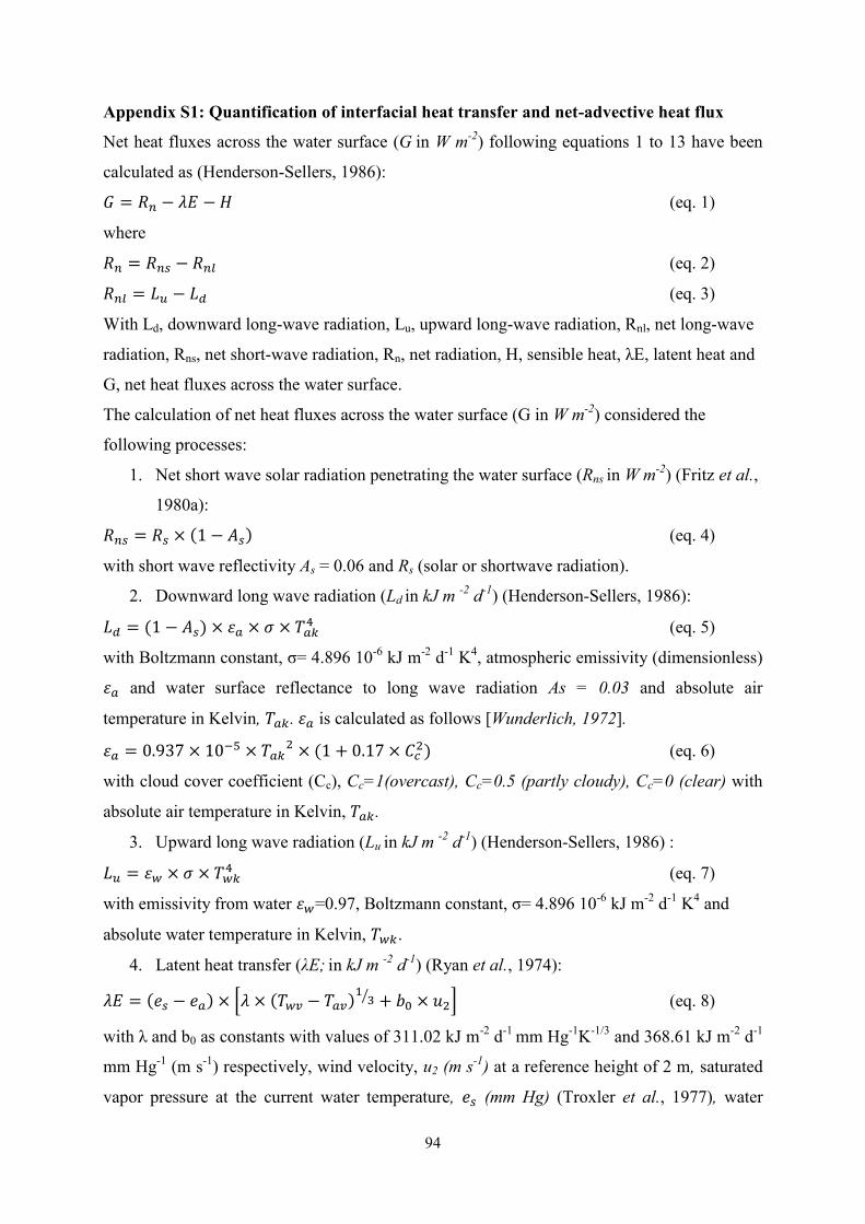
94
Appendix S1: Quantification of interfacial heat transfer and net-advective heat flux
Net heat fluxes across the water surface (G in W m-2
) following equations 1 to 13 have been
calculated as (Henderson-Sellers, 1986):
𝐺 = 𝑅𝑛 − 𝜆𝐸 − 𝐻 (eq. 1)
where
𝑅𝑛 = 𝑅𝑛𝑠 − 𝑅𝑛𝑙 (eq. 2)
𝑅𝑛𝑙 = 𝐿𝑢 − 𝐿𝑑 (eq. 3)
With Ld, downward long-wave radiation, Lu, upward long-wave radiation, Rnl, net long-wave
radiation, Rns, net short-wave radiation, Rn, net radiation, H, sensible heat, λE, latent heat and
G, net heat fluxes across the water surface.
The calculation of net heat fluxes across the water surface (G in W m-2
) considered the
following processes:
1. Net short wave solar radiation penetrating the water surface (Rns in W m-2
) (Fritz et al.,
1980a):
𝑅𝑛𝑠 = 𝑅𝑠 × (1 − 𝐴𝑠) (eq. 4)
with short wave reflectivity As = 0.06 and Rs (solar or shortwave radiation).
2. Downward long wave radiation (Ld in kJ m -2
d-1
) (Henderson-Sellers, 1986):
𝐿𝑑 = (1 − 𝐴𝑠) × 𝜀𝑎 × 𝜎 × 𝑇𝑎𝑘4 (eq. 5)
with Boltzmann constant, σ= 4.896 10-6
kJ m-2
d-1
K4, atmospheric emissivity (dimensionless)
𝜀𝑎 and water surface reflectance to long wave radiation As = 0.03 and absolute air
temperature in Kelvin, 𝑇𝑎𝑘. 𝜀𝑎 is calculated as follows [Wunderlich, 1972].
𝜀𝑎 = 0.937 × 10⁻⁵ × 𝑇𝑎𝑘2 × (1 + 0.17 × 𝐶𝑐
2) (eq. 6)
with cloud cover coefficient (Cc), Cc=1(overcast), Cc=0.5 (partly cloudy), Cc=0 (clear) with
absolute air temperature in Kelvin, 𝑇𝑎𝑘.
3. Upward long wave radiation (Lu in kJ m -2
d-1
) (Henderson-Sellers, 1986) :
𝐿𝑢 = 𝜀𝑤 × 𝜎 × 𝑇𝑤𝑘4 (eq. 7)
with emissivity from water 𝜀𝑤=0.97, Boltzmann constant, σ= 4.896 10-6
kJ m-2
d-1
K4 and
absolute water temperature in Kelvin, 𝑇𝑤𝑘.
4. Latent heat transfer (λE; in kJ m -2
d-1
) (Ryan et al., 1974):
𝜆𝐸 = (𝑒𝑠 − 𝑒𝑎) × [𝜆 × (𝑇𝑤𝑣 − 𝑇𝑎𝑣)1
3⁄ + 𝑏0 × 𝑢2] (eq. 8)
with λ and b0 as constants with values of 311.02 kJ m-2
d-1
mm Hg-1
K-1/3
and 368.61 kJ m-2
d-1
mm Hg-1
(m s-1
) respectively, wind velocity, u2 (m s-1
) at a reference height of 2 m, saturated
vapor pressure at the current water temperature, 𝑒𝑠 (mm Hg) (Troxler et al., 1977), water

Mesocosm experiments identifying hotspots of groundwater upwelling in a water column by fiber
optic distributed temperature sensing
95
vapor pressure immediately above the mesocosm surface, 𝑒𝑎 (mm Hg) (Troxler et al., 1977),
Twv and Tav are the virtual water and air temperatures respectively (°K) (Ryan et al., 1974):
𝑒𝑠 = 25.37 × 𝑒𝑥𝑝 [17.62 −5271
𝑇𝑤𝑘] (eq. 9)
with absolute water temperature in Kelvin, 𝑇𝑤𝑘.
𝑒𝑎 = 𝑅ℎ × 25.37𝑒𝑥𝑝 [17.62 −5271
𝑇𝑎𝑘] (eq. 10)
with Rh, relative humidity in decimal fraction and absolute air temperature in Kelvin, 𝑇𝑎𝑘.
𝑇𝑤𝑣 = (𝑇𝑤𝑘
[1.0−(0.378×𝑒𝑠/𝑃)]) (eq. 11)
with P= barometric pressure (mm Hg) which was assumed to be equivalent to one atmosphere
(760 mm Hg) for the current study.
𝑇𝑎𝑣 = (𝑇𝑎𝑘
[1.0−(0.378×𝑒𝑎/𝑃)]) (eq. 12)
5. Sensible heat transfer (H in kJ m -2
d-1
) (Ryan et al., 1974):
𝐻 = 𝜆𝐸 × 0.61 × 10⁻³𝑃 ×(𝑇𝑤𝑘−𝑇𝑎𝑘)
(𝑒𝑠−𝑒𝑎) (eq. 13)
Change in internal energy (E, in J) over a time interval ∆𝑡 related to components of the net
heat fluxes across the water surface (G) is calculated as:
𝐸𝑅𝑛𝑠 = 𝑅𝑛𝑠 × 𝐴0 × ∆𝑡 (eq. 14)
𝐸𝐿𝑑 = 𝐿𝑑 × 𝐴0 × ∆𝑡 (eq. 15)
𝐸𝐿𝑢 = 𝐿𝑢 × 𝐴0 × ∆𝑡 (eq. 16)
𝐸𝜆𝐸 = 𝜆𝐸 × 𝐴0 × ∆𝑡 (eq. 17)
𝐸𝐻 = 𝐻 × 𝐴0 × ∆𝑡 (eq. 18)
𝐴0 = 2∆z∆x + 2∆z∆y + ∆x∆y (eq. 19)
With 𝐴0= area (m2), ∆𝑥=length (m), ∆𝑦=width (m) and ∆𝑧=height (m).
At t=0 the internal energy within the control volume is:
𝐸𝑡=0 = 𝜌 × (∆𝑥∆𝑦∆𝑧) × 𝑈𝑡=0 (eq. 20)
At t=∆t the internal energy within the control volume is:
𝐸𝑡=∆𝑡 = 𝜌 × (∆𝑥∆𝑦∆𝑧) × 𝑈𝑡=∆𝑡 (eq. 21)
With U, Internal energy per unit mass of fluid (J kg-1
).
Therefore, change on internal energy within the control volume is:
∆𝐸 = 𝜌 × (∆𝑥∆𝑦∆𝑧) × ∆𝑈 (eq. 22)
Where
∆𝑈 = 𝑈𝑡=∆𝑡 − 𝑈𝑡=0 (eq. 23)

96
By conservation of energy:
∆𝐸 = 𝐸𝑖𝑛 − 𝐸𝑜𝑢𝑡 + 𝐸𝑔𝑤 − 𝐸ℎ𝑏 − 𝐸𝐻 − 𝐸𝜆𝐸 + 𝐸𝑅𝑛𝑠 + 𝐸𝐿𝑑 − 𝐸𝐿𝑢 (eq. 24)
where, Ein, advected anergy in the control volume by inflow water, Eout, advected energy out
of the control volume by outflow water, Egw, advected energy in the control volume by
simulated groundwater injection and Ehb, energy by sediment conduction.
For a system that performs a small amount of work on its surroundings, the change in internal
energy manifests as a change in temperature:
𝑑𝑈 = 𝐶𝑝 × 𝑑𝑇 (eq. 25)
∆𝑈 ≈ 𝐶𝑝 × ∆𝑇 (eq. 26)
With heat capacity, Cp= 4180 J kg-1
°C-1
, ∆𝑇 and 𝑑𝑇, change of temperature.
Therefore, change in internal energy can be expressed as:
∆𝐸 ≅ 𝜌 × ∑ (∆𝑥∆𝑦∆𝑧) × 𝐶𝑝 × ∆𝑇𝑖𝑁𝑚𝑖=1 (eq. 27)
Where Nm=1944, total number of FO-DTS measurement locations, i, each measurement
location, ∆𝑥∆𝑦∆𝑧 (m3), control volume of each FO-DTS measurement, density of water, ρw =
103 kg m
-3 and ∆𝑇𝑖, change of temperature over the interval ∆𝑡 in location i.
Going back to equation 24 and grouping together the atmospheric components of energy into
a single term; EG, energy transferred across the interface:
𝐸𝐺 = −𝐸𝐻 − 𝐸𝜆𝐸 + 𝐸𝑅𝑛𝑠 + 𝐸𝐿𝑑 − 𝐸𝐿𝑢 (eq. 28)
Now change of internal energy can be expressed as,
∆𝐸 = 𝐸𝑖𝑛 − 𝐸𝑜𝑢𝑡 + 𝐸𝑔𝑤 − 𝐸ℎ𝑏 + 𝐸𝐺 (eq. 29)
And the sum of the total advected energy can be calculated as,
∆𝐸 − 𝐸𝐺 = 𝐸𝑖𝑛 − 𝐸𝑜𝑢𝑡 + 𝐸𝑔𝑤 (eq. 30)
References appendix S1
Fritz JJ, Meredith DD, Middleton AC. 1980. Non-steady state bulk temperature determination
for stabilization ponds. Water Research 14: 413–420 DOI: 0043-1354/80/0501-
0413502.00/0
Henderson-Sellers B. 1986. Calculating the surface energy balance for lake and reservoir
modeling: A review. Reviews of Geophysics 24 (3): 625 DOI:
10.1029/RG024i003p00625
Ryan PJ, Harleman DRF, Stolzenbach KD. 1974. Surface Heat Loss From Cooling Ponds.
Water Resources Research 10 (5)
Troxler RW, Thackston EL, Robert W. 1977. Predicting the Rate of Warming of Rivers

Mesocosm experiments identifying hotspots of groundwater upwelling in a water column by fiber
optic distributed temperature sensing
97
below Hydroelectric Installations. Water Environment Federation 49 (8): 1902–1912
Wunderlich, W.O. 1972. Heat and mass transfer between a water surface and the atmosphere.
Lab. Report No. 14, Tennessee Valley Authority Engineering Laboratories, Norris, TN.
Cited by: Nath, S.S., 1996. Development of a Decision Support System for Pond
Aquaculture. Oregon State University.
Appendix S2 Nomenclature
G (W m-2
): net heat fluxes across the water surface.
Ld (kJ m -2
d-1
): downward long-wave radiation
Lu (kJ m -2
d-1
): upward long-wave radiation
Rnl (kJ m -2
d-1
): net long-wave radiation
Rns (W m-2
): net short-wave radiation
Rn (W m-2
): net radiation
H (kJ m -2
d-1
): sensible heat
λE (kJ m -2
d-1
): latent heat.
As (dimensionless): short wave reflectivity
Rs (W m-2
): solar or shortwave radiation.
σ (kJ m -2
d-1
k-4
): Boltzmann constant.
εa (dimensionless): atmospheric emissivity.
As (dimensionless): water surface reflectance to long wave radiation.
Tak (Kelvin): absolute air temperature in Kelvin.
Cc (dimensionless): cloud cover coefficient.
εw (dimensionless): emissivity from water.
Twk (Kelvin): absolute water temperature.
λ (kJ m-2
d-1
mm Hg-1
K-1/3
): constant
b0 (kJ m-2
d-1
mm Hg-1
(m s-1
) ): constant.
u2 (m s-1
): wind velocity, at a reference height of 2 m.
es (mm Hg): saturated vapor pressure at the current water temperature.
ea (mm Hg): water vapor pressure immediately above the pond surface.
Twv (Kelvin): virtual water temperatures.
Tav (Kelvin): virtual air temperatures.
Rh (dimensionless): relative humidity in decimal fraction.
P (mm Hg): barometric pressure.
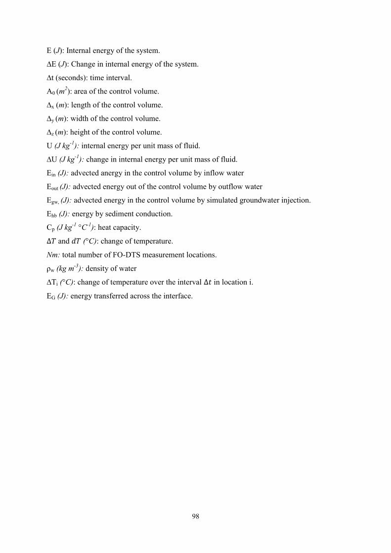
98
E (J): Internal energy of the system.
∆E (J): Change in internal energy of the system.
∆t (seconds): time interval.
A0 (m2): area of the control volume.
∆x (m): length of the control volume.
∆y (m): width of the control volume.
∆z (m): height of the control volume.
U (J kg-1
): internal energy per unit mass of fluid.
∆U (J kg-1
): change in internal energy per unit mass of fluid.
Ein (J): advected anergy in the control volume by inflow water
Eout (J): advected energy out of the control volume by outflow water
Egw, (J): advected energy in the control volume by simulated groundwater injection.
Ehb (J): energy by sediment conduction.
Cp (J kg-1
°C-1
): heat capacity.
∆𝑇 and 𝑑𝑇 (°C): change of temperature.
Nm: total number of FO-DTS measurement locations.
ρw (kg m-3
): density of water
∆Ti (°C): change of temperature over the interval ∆𝑡 in location i.
EG (J): energy transferred across the interface.

Mesocosm experiments identifying hotspots of groundwater upwelling in a water column by fiber optic distributed temperature sensing
99
Figure S1 Comparison of LISA maps and spatial correlation coefficients between layer 1 and 2 and
layer 1 and 3 for datasets: a) 1 L min-1 clear conditions, daytime, b) 1 L min-1 partly cloudy conditions,
daytime and c) 1 L min-1 partly cloudy conditions, night-time. From top row to bottom row: layer 4,
layer 3, layer 2 and layer 1.

100
Table S1 Spatial correlation coefficients between layers.
Day Night
Layer
n° 1 2 3 4 1 2 3 4
1 L min-1
Clear
1 1 0.39808 0.51153 0.14203 1 0.73808 0.51705 -0.8551
2 0.39808 1 0.24951 0.05932 0.73808 1 0.50801 -0.18037
3 0.51153 0.24951 1 0.04728 0.51705 0.50801 1 -0.11156
4 0.14203 0.05932 0.04728 1 -0.8551 -0.18037 -0.11156 1
1 L min-1
Partly
cloudy
1 1 0.24911 0.45869 -0.1161 1 0.37761 0.51711 0.28616
2 0.24911 1 0.58511 0.61316 0.37761 1 0.54338 0.41679
3 0.45869 0.58511 1 0.28031 0.51711 0.54338 1 0.50589
4 -0.1161 0.61316 0.28031 1 0.28616 0.41679 0.50589 1
1 L min-1
Overcast
1 1 0.41457 0.48095 0.42329 1 0.74711 0.6806 0.5718
2 0.41457 1 0.60944 0.66255 0.74711 1 0.72155 0.60979
3 0.48095 0.60944 1 0.81466 0.6806 0.72155 1 0.83116
4 0.42329 0.66255 0.81466 1 0.5718 0.60979 0.83116 1
5.5 L min-1
Clear
1 1 0.51591 0.32147 0.17959 1 0.64121 0.47728 0.13437
2 0.51591 1 0.59571 0.56061 0.64121 1 0.75321 0.11554
3 0.32147 0.59571 1 0.68505 0.47728 0.75321 1 0.23392
4 0.17959 0.56061 0.68505 1 0.13437 0.11554 0.23392 1
5 L min-1
Overcast
1 1 0.79544 0.63641 0.54602 1 0.75846 0.60806 0.42685
2 0.79544 1 0.88935 0.79137 0.75846 1 0.87773 0.68253
3 0.63641 0.88935 1 0.93334 0.60806 0.87773 1 0.8936
4 0.54602 0.79137 0.93334 1 0.42685 0.68253 0.8936 1
15 L min-1
Overcast
1 1 0.84675 0.65938 0.26386 1 0.85239 0.68532 0.28563
2 0.84675 1 0.88841 0.40424 0.85239 1 0.89219 0.44944
3 0.65938 0.88841 1 0.45033 0.68532 0.89219 1 0.50333
4 0.26386 0.40424 0.45033 1 0.28563 0.44944 0.50333 1

Mesocosm experiments identifying hotspots of groundwater upwelling in a water column by fiber
optic distributed temperature sensing
101

102
4 Thermal infrared imaging for detection of groundwater at the surface of stagnant
freshwater bodies
Amaya I. Marruedo Arricibitaa,b, Stephen J. Dugdalec, Stefan Krausec, David M.
Hannahc and Jörg Lewandowskia
a Department of Ecohydrology, Leibniz-Institute of Freshwater Ecology and Inland Fisheries,
12587 Berlin, Germany.
b Department of Geography, Humboldt University of Berlin, 10099 Berlin, Germany.
c School of Geography, Earth and Environmental Sciences, University of Birmingham, B15
2TT Birmingham, United Kingdom.
Published in: Journal of Hydrology
Marruedo Arricibita AI, Dugdale SJ, Krause S, Hannah DM, Lewandowski J. 2018. Thermal
infrared imaging for the detection of relatively warm lacustrine groundwater discharge at the
surface of freshwater bodies. Journal of Hydrology 562: 281–289 DOI:
10.1016/j.jhydrol.2018.05.004
Received 24 October 2017; Received in revised form 29 April 2018; Accepted 3 May 2018
Available online 04 May 2018
0022-1694/ © 2018 Elsevier B.V. All rights reserved.
Only for non-commercial use.

Thermal infrared imaging for detection of groundwater at the surface of stagnant freshwater bodies
103
Abstract
Thermal infrared (TIR) imaging has been previously applied to survey relatively large thermal
footprints in coastal zones, lakes, reservoirs and rivers. In freshwater systems, the buoyancy
of relatively warm groundwater during the winter months allows for the surface identification
of groundwater discharge or thermal pollution using TIR imaging. However, information
regarding the performance of TIR for resolving this warm groundwater upwelling is limited,
particularly at fine spatial scales and variable discharge rates. In order to evaluate the
suitability of TIR to trace warm groundwater upwelling at the water surface of lakes, ponds
and reservoirs (e.g. lacustrine groundwater discharge (LGD) in shallow near-shore zones) we
conducted a mesocosm experiment with a TIR camera situated 4 m above the water surface to
capture thermal patterns in response to different groundwater discharge rates, weather
conditions and the diurnal cycle. A fiber optic distributed temperature sensing system (FO-
DTS) installed at 2 cm below the water surface was used to ground-truth spatial patterns
observed in TIR images. Results show the impacts of both the diurnal cycle of net radiation
and prevailing weather conditions on the accuracy of TIR imaging for resolving warm
groundwater discharge. Most reliable results were obtained under overcast weather conditions
and during the night. The results of our study provide guidance for those looking to use TIR
for conducting thermal tracing of LGD at the surface of freshwater bodies during winter.
Keywords: TIR, FO-DTS, groundwater, lake, heat tracing, leakage

104
4.1 Introduction
The use of thermal infrared (TIR) remote sensing is increasingly popular in the earth and
environmental sciences for mapping of temperature patterns and thermal anomalies in water
bodies (Dugdale, 2016). As such, TIR imaging has been applied in a wide range of contexts
for monitoring of naturally occurring natural processes such as submarine groundwater
discharge (SGD) in coastal areas (Johnson et al., 2008; Lee et al., 2016; Tamborski et al.,
2015), groundwater discharge in streams and lakes (Hare et al., 2015; Wawrzyniak et al.,
2016), volcanic activity (Davies et al., 2008) or hydrothermal systems (Neale et al., 2016). It
is also used for the identification of anthropogenic impacts on hydrological systems including
thermal effluent from power plants (Wang et al., 2016) and surface water contamination by
illegal sewers or storm drainage (Lega and Napoli, 2010).
TIR imaging allows for the measurement of water surface temperature at high spatial
resolution across a wide range of scales (Dugdale, 2016). While TIR has been relatively
under-used until recently (in comparison to other remote sensing techniques), the increasing
affordability of TIR has led to a recent uptake of this technology. This increased use of TIR
has driven a range of literature reviewing the technological applications and limitations of
satellite, airborne and ground-based TIR remote sensing (e.g. Dugdale, 2016; Handcock et al.,
2012; Mundy et al., 2017; Sobrino et al., 2016) for the monitoring and mapping of water
temperature anomalies in both marine and freshwater environments.
In marine systems, Submarine Groundwater Discharge (SGD) is a major source of nutrients
and other chemical components (Burnett et al., 2006, 2003; Danielescu and MacQuarrie,
2011; Johnson et al., 2008; Taniguchi et al., 2002). SGD is known to affect water quality and
phytoplankton dynamics, potentially leading to environmental phenomena such as
eutrophication and algal blooms (Anderson et al., 2002; Hu et al., 2006; Lee and Kim, 2007).
In freshwater systems, groundwater discharge can create discrete temperature anomalies that
serve as thermal refugia for fish and other ectothermic species (Baker et al., 2014; Brabrand et
al., 2002; Hayashi and Rosenberry, 2002; Warren et al., 2005). Groundwater discharge can
also impact nutrient budgets of lentic ecosystems (Boulton et al., 1998; Meinikmann et al.,
2013; Shaw et al., 1990) and may play a role as a potential vector for pollution in streams and
lakes (Nakayama and Watanabe, 2008).
Due to the importance of groundwater discharge in marine and freshwater systems, the
literature abounds with TIR remote sensing-based methods for the detection of diffuse and
discrete groundwater discharge. In marine systems, Johnson et al. (2008) demonstrated that

Thermal infrared imaging for detection of groundwater at the surface of stagnant freshwater bodies
105
TIR imagery is an appropriate tool for mapping SGD. More recently, Tamborski et al. (2015)
combined airborne TIR with radium (223,224
Ra) and radon (222
Rn) surface water sample
collection to quantify diffuse SGD. Similarly, Lee et al. (2016) demonstrated how combining
aerial TIR imagery with field observations can be used to identify large groundwater inputs
from coastal aquifers to the ocean. In freshwater environments, Schuetz and Weiler (2011)
used ground based TIR thermography to detect discrete groundwater discharge into streams.
A similar experiment by Briggs et al. (2016) demonstrated how ground-based TIR can reveal
fine scale groundwater discharge patterns which would have not been resolved by other
(coarser) methodologies. At larger scales, Wawrzyniak et al. (2016) used airborne TIR to
resolve cold water patches in a riverine system as a function of the temperature difference
between the river (in low flow conditions) and groundwater inputs.
Groundwater detection using TIR is more straightforward in marine than freshwater
environments due to the large density difference between groundwater inflow and the saline
water column. Unlike in marine environments, where these salinity differences drive SGD
upwelling, groundwater upwelling in freshwater systems is largely driven by temperature.
Even small temperature differences may provoke groundwater-surface water density gradients
that approach levels of buoyancy similar to that of groundwater discharge in saline systems
(Lewandowski et al., 2013). This buoyancy, amongst other factors, enables the detection of
groundwater upwelling at the surface of freshwater bodies. However, because the
groundwater-surface water temperature difference can vary substantially, the ability of TIR to
resolve groundwater upwelling is less consistent than in marine systems. While many
publications (e.g. Briggs et al., 2016, 2013; Danielescu et al., 2009; Dugdale et al., 2015;
Tcherepanov et al., 2005; Wawrzyniak et al., 2016) document the use of TIR to detect
groundwater upwelling in freshwater bodies, the vast majority of these studies focus on the
detection of cool thermal anomalies in summer, with relatively little attention paid to the
quantification of warm groundwater-surface water exchanges in winter. Furthermore, the
examples that do exist which describe TIR imaging to detect winter groundwater upwelling in
freshwater environments focus on groundwater discharge: (i) in streams (e.g. Hare et al.,
2015; Wirth et al., 2012); (ii) at marine beaches (Röper et al., 2014) and; (iii) in vernal and
peatland pools (Frisbee et al., 2016), rather than in lentic waterbodies where mixing patterns
are substantially different.
In addition, while previous studies (e.g. Briggs et al., 2016; Dugdale et al., 2015; Hare et al.,
2015; Schuetz et al., 2012; Schuetz and Weiler, 2011) highlight the reasonable ability of TIR

106
remote sensing to detect thermal anomalies related to groundwater discharge in real world
freshwater environments, there remains a lack of formal ‘laboratory-style’ data evaluating the
precise hydrological (e.g. discharge rates) and meteorological (e.g. weather conditions)
conditions under which TIR remote sensing best detects groundwater upwelling, especially
during the winter season.
In light of this these knowledge gaps, we present the results of a mesocosm experiment
designed to test the suitability of TIR for tracing the upwelling of discrete lacustrine
groundwater discharge (LGD) in lentic waterbodies (e.g. in shallow near-shore zones of lakes,
ponds and small reservoirs). Our specific objectives were: (i) to compare (both visually and
quantitatively) TIR observations of surface water temperature with simultaneously-collected
FO-DTS temperature data measured 2 cm below the water surface and (ii) to evaluate the
suitability of ground-based TIR for the detection of spatial patterns in relatively warm
groundwater upwelling as a function of different discharge rates, weather conditions and the
diurnal cycle.
4.2 Methods
4.2.1 Experimental design
The mesocosm used in this study contained two inlets and one outlet (Fig. 4.1). Water from
Lake Müggelsee located in Berlin, Germany (mean of 4.7 °C over the course of the
experiment) was injected into the corner of the mesocosm via one of the inlets (rate ≈33 L
min−1
). The inlet remained open at all times to keep water temperatures well-mixed and
relatively constant. The other inlet was installed at the base of the mesocosm and used for
controlled warm water injections. A hosepipe was connected to this inlet to provide warm
water. The pipe was insulated with foam to reduce cooling along the flow path from the tap to
the mesocosm (approximately 65 m). Temperature of the injected flow (measured at halfway
between the tap and mesocosm) ranged from 14 to 16 °C. A nozzle was connected to the end
of the inlet and covered with sediment to realistically simulate dispersal of the injected water
through a layer of sediment. Finally, an outlet at the other side of the mesocosm was used to
maintain a constant water level of 0.82 m. Discharge at this outlet varied from 34 to 48 L
min−1
depending on the warm water injection rate (Marruedo Arricibita et al., 2018).
For the FO-DTS surveys, an aluminium frame of dimensions 4 m ×2 m × 1.5 m (Fig. 4.1) was
installed within the mesocosm. The aluminium frame was used to support the FO cable in a
grid-like pattern 2 cm below the water surface (Fig. 4.1). The FO cable grid consisted of 15
lines (rows) of cable spaced 12.5 cm apart. An ULTIMA-S DTS (SILIXA Ltd.) instrument

Thermal infrared imaging for detection of groundwater at the surface of stagnant freshwater bodies
107
with a sampling resolution of 12.5 cm was used for the FO-DTS surveys. This experimental
setup essentially resulted in gridded temperature measurements with a resolution of 12.5 cm.
Temperatures were acquired with a temporal frequency of 10 s (mean of the preceding 10 s
period; essentially the integration time of the FO-DTS). 500 m of 2.8 mm diameter Corning
ClearCurve simplex fibre (loose tube, 1 multimode fibre, both ends terminated with
E2000/APC connectors) were deployed for the experiments. This selected FO cable
specification allowed bending and was thus appropriate for installation in the aluminium
frame (Marruedo Arricibita et al., 2018).
Thermal images were acquired from a TIR camera installed 4 m above the mesocosm on a
steel frame (Fig. 4.1) and oriented perpendicular to the water surface. The FO-DTS
measurements were used for ground truthing of the TIR results which only capture direct
surface temperatures (ie. the upper 10 μm of the water surface; Torgersen et al., 2001). We
used a VarioCAM® hr head camera (InfraTec GmbH) with 640 ×480 pixels (7.5–14 μm). The
camera was equipped with a wide angle lens with focal length of 12.5 mm and field of view
(FOV) 65° × 51°. The temperature measurement range is −40 to 1200 °C and reported
measurement accuracy is ±2 °C or ± 2%.
Figure 4.1 Schematic of the mescocosm experimental design including TIR setup and the upper layer
of the FO-DTS.

108
4.2.2 Measurement protocol and calibration
FO-DTS
Calibration of the FO-DTS was carried out using reference sections of fibre optic cable
immersed within ice baths containing a mix of ice and water (maintained at ∼0.2 °C). The
first and last 20 m of fibre optic cable were submerged in this well mixed ice bath, and an
external temperature probe connected to the DTS device used to monitor calibration bath
temperatures independently. For differential loss corrections, fixed value settings were chosen
along the relatively short cable (500 m) without any splices (Marruedo Arricibita et al., 2018).
A default value of 0.255 dB/km was used. This is the expected value for Corning ClearCurve
OM3 fibre. A two-way single-ended measurement setup was deployed with alternating
bidirectional monitoring of the light pulse sent from the DTS device (Krause and Blume,
2013).
TIR
The TIR camera used in this study has an uncooled microbolometer FPA detector (uncooled
Focal Plane Array) with an internal shutter. Small alterations in the microbolometer
manufacturing process lead to non-homogeneous pixel specific sensor parameters which can
induce temperature non-uniformities in the image (Tempelhahn et al., 2016, 2015). The
camera’s non-uniformity correction system (NUC) compensates for these minor sources of
error by using an internal optical shutter that periodically covers the whole camera field of
view to provide a reference temperature. In this manner, the TIR camera performed a NUC
(also known as a Flat Field Correction) every 90 s to correct for temperature or thermal drift
effects on the measurements (eg. Dugdale, 2016; Handcock et al., 2012; Tempelhahn et al.,
2015, 2016; Zuo et al., 2011).
A simple MATLAB function was developed to compensate for the effects of vignetting which
created a minor systematic radial temperature gradient in the raw TIR images. This was
achieved by applying a convolution filter with a smoothing window of 25 pixels to the raw
imagery and subsequently creating a new image whereby each pixel is assigned a value equal
to the difference between its smoothed value and the mean of all pixels within the image. The
resulting raster essentially contained an inverse image of the vignetting effect which was then
subtracted from the raw TIR image resulting in a final corrected TIR image.
Since the aim of the present study is to evaluate the suitability of TIR to determine spatial
patterns of warm water upwelling, rather than quantifying rates of upwelling per se, absolute
temperatures were not of specific interest and were not calculated for the data obtained by the

Thermal infrared imaging for detection of groundwater at the surface of stagnant freshwater bodies
109
TIR camera. Instead, we compared the TIR-derived data to the FO-DTS observations by
computing the difference in minimum temperature (ΔTmin) observed by the (corrected) TIR
image and the FO-DTS device.
4.2.3 Study period and influence of discharge rates, weather conditions and
diurnal cycle
Six 24-h temperature datasets of simultaneously-acquired FO-DTS and TIR data were used in
the present study (Table 4.1). The temperature datasets were obtained during 11–27 March
2015. In order to assess the performance of the TIR methodology at different discharge rates
and weather conditions, injection rates were varied between 1, 5 and 15 L min−1
under a range
of different (ie overcast and clear) sky conditions. Overcast vs. clear weather conditions were
inferred from data acquired from a weather station installed alongside the mesocosm,
whereby relative solar radiation was defined as the ratio of observed shortwave radiation
(measured by the weather station pyranometer) to the computed maximum solar radiation that
would be expected using clear sky conditions (after Allan et al., 1998). For example, average
relative shortwave radiation measured on 26 March 2015 of 0.17 was considered ‘overcast’
whereas the value on 19 March 2015 of 0.97 was classified as clear. Performance of the TIR
methodology was examined at different points throughout the diurnal cycle to evaluate
differences between day and night conditions.
Table 4.1 24-hour measurements with FO-DTS and TIR camera. The control dataset is only used as a
reference for the initial conditions of the mesocosm measurements and is not included in the results.
Injection rate (L min-1
) Weather conditions Date (in March 2015)
0 (control) overcast 11
1 clear 19
1 overcast 26
5 clear 18
5 overcast 27
15 overcast 12

110
4.2.4 Comparison of TIR temperature data with FO-DTS temperature data
We assessed the performance of the TIR data for locating and measuring the spatial extent of
warm groundwater upwelling by comparing the TIR data with FO-DTS. Because the TIR
images essentially contain multiple ‘layers’ of radiation resulting from solar radiation and/ or
longwave reflections (from trees, clouds, etc), it is necessary to determine the extent to which
the temperature signal from the warm water discharge matches that recorded by the FO-DTS
data, in light of these other sources of noise. This was accomplished both visually and
quantitatively.
Visual comparison
A direct comparison of the FO-DTS and TIR thermal image data was difficult, given the
different spatial resolutions of both methods and the fact that FO-DTS provided a spatially
integrated temperature along a 2dimensional cable section while TIR produced gridded
temperature data. To enable comparison between the TIR and FO-DTS data, the portion of the
TIR image corresponding to the extent of the FO-DTS measurements was extracted from the
TIR images of the mesocosm. The TIR images were then down sampled to the same
resolution of the FODTS temperature data matrix, allowing the resulting 30 × 15 pixel TIR
matrices to be compared to the FO-DTS grid.
We visually compared the average temperature grids generated by the FO-DTS and TIR
approaches for the first 3.5 min of each hour. Although the FO-DTS temperature data showed
clearer spatial temperature patterns when averaged over longer periods of time, this was not
the case for the temperature data monitored by the TIR camera, presumably due to increased
surface movement in comparison to the FO-DTS (submerged at 2 cm below the surface).
Indeed, averaging the TIR temperature data over long periods of time resulted in overly
blurred or smoothed patterns. Therefore, the decision to focus on the 3.5 min period
represented a compromise between the two methods.
Temperature anomalies caused by external factors such as leaves, branches or ducks on the
water surface were identified and masked out before plotting the resulting temperature grids
for the FO-DTS and TIR data. Temperature values found to be outside of 3 standard
deviations above or below the mean were considered outliers due to external factors and were
also removed.
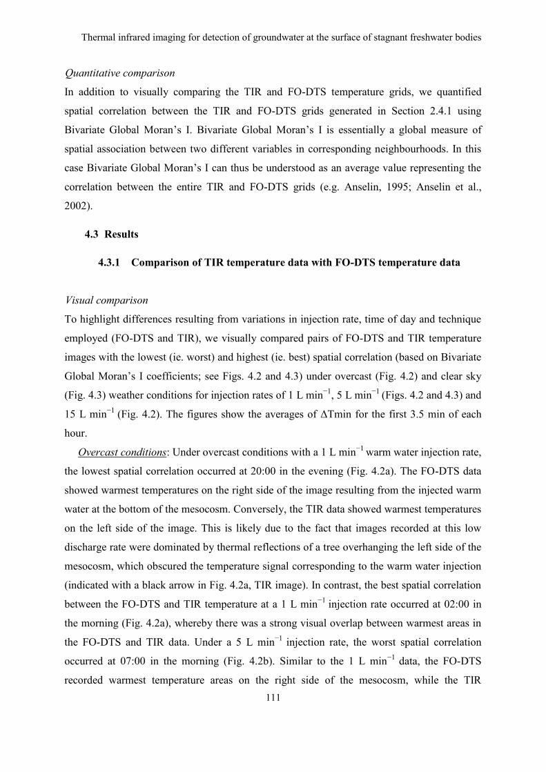
Thermal infrared imaging for detection of groundwater at the surface of stagnant freshwater bodies
111
Quantitative comparison
In addition to visually comparing the TIR and FO-DTS temperature grids, we quantified
spatial correlation between the TIR and FO-DTS grids generated in Section 2.4.1 using
Bivariate Global Moran’s I. Bivariate Global Moran’s I is essentially a global measure of
spatial association between two different variables in corresponding neighbourhoods. In this
case Bivariate Global Moran’s I can thus be understood as an average value representing the
correlation between the entire TIR and FO-DTS grids (e.g. Anselin, 1995; Anselin et al.,
2002).
4.3 Results
4.3.1 Comparison of TIR temperature data with FO-DTS temperature data
Visual comparison
To highlight differences resulting from variations in injection rate, time of day and technique
employed (FO-DTS and TIR), we visually compared pairs of FO-DTS and TIR temperature
images with the lowest (ie. worst) and highest (ie. best) spatial correlation (based on Bivariate
Global Moran’s I coefficients; see Figs. 4.2 and 4.3) under overcast (Fig. 4.2) and clear sky
(Fig. 4.3) weather conditions for injection rates of 1 L min−1
, 5 L min−1
(Figs. 4.2 and 4.3) and
15 L min−1
(Fig. 4.2). The figures show the averages of ΔTmin for the first 3.5 min of each
hour.
Overcast conditions: Under overcast conditions with a 1 L min−1
warm water injection rate,
the lowest spatial correlation occurred at 20:00 in the evening (Fig. 4.2a). The FO-DTS data
showed warmest temperatures on the right side of the image resulting from the injected warm
water at the bottom of the mesocosm. Conversely, the TIR data showed warmest temperatures
on the left side of the image. This is likely due to the fact that images recorded at this low
discharge rate were dominated by thermal reflections of a tree overhanging the left side of the
mesocosm, which obscured the temperature signal corresponding to the warm water injection
(indicated with a black arrow in Fig. 4.2a, TIR image). In contrast, the best spatial correlation
between the FO-DTS and TIR temperature at a 1 L min−1
injection rate occurred at 02:00 in
the morning (Fig. 4.2a), whereby there was a strong visual overlap between warmest areas in
the FO-DTS and TIR data. Under a 5 L min−1
injection rate, the worst spatial correlation
occurred at 07:00 in the morning (Fig. 4.2b). Similar to the 1 L min−1
data, the FO-DTS
recorded warmest temperature areas on the right side of the mesocosm, while the TIR

112
temperature data again indicated warmest temperatures on the left due to reflections from tree
cover. The best calculated spatial correlation between FO-DTS and TIR temperature data
occurred at 02:00 in the morning (Fig. 4.2b), whereby the FO-DTS and TIR data show a
similar extent of warm water. Under an injection rate of 15 L min−1
, the worst spatial
correlation between FO-DTS and TIR temperature data occurred at 13:00 in the afternoon
(Fig. 4.2c), while the best correlation occurred at 20:00 (Fig. 4.2c). Unlike the lower injection
rates, both cases showed a good degree of visual similarity between the FO-DTS and TIR
temperature grids. Taken together, these results indicate a reasonable degree of similarity
between the FO-DTS and TIR data, particularly for the higher injection rates. The TIR signal
corresponding to the warm water injection was also clearer at night-time than during the day.
Clear sky conditions: Under clear sky conditions (Fig. 4.3), simulated groundwater
upwelling produced by the warm water injection was generally not detected by TIR. Fig. 4.3
shows the FO-DTS and TIR temperature grids corresponding to the lowest and highest spatial
correlations. The overall correlation between FO-DTS and TIR was systematically lower than
under overcast skies, and no meaningful differences were observed between the computed
worst and best spatial correlation values. Thus, there was little visual agreement between the
TIR and FO-DTS data for any injection rate, throughout the entire diurnal cycle (see Fig. 4.3a
and b).

Thermal infrared imaging for detection of groundwater at the surface of stagnant freshwater bodies
113
Figure 4.2 Visual comparison of TIR temperature data with FO-DTS temperature data. Worst (left) and best
(right) spatially correlated datasets for overcast conditions at three injection rates: a) 1 L min−1
, b) 5 L min−1
and
c) 15 L min−1
. Temperature signal corresponding to the warm water injection is indicated with a black arrow in
Fig. 4.2a and b.

114
Figure 4.3 Visual comparison of TIR temperature data with FO-DTS temperature data. Worst (left)
and best (right) correlated datasets for clear conditions at three injection rates: a) 1 L min−1
and b) 5 L
min−1
.
Quantitative comparison
We calculated Global Moran’s I coefficients between FO-DTS and TIR temperature data
under overcast (Fig. 4.4) and clear conditions (Fig. 4.5) across the entire 24-h long
measurement cycle and for all simulated warm water injection rates (Figs. 4.4 and 4.5: a) 1 L
min−1
and b) 5 L min−1
and Fig. 4c: 15 L min−1
) with a view to ascertaining the time and
conditions associated with the best and worst performance of the TIR methodology.
Generally, we observed that Global Moran’s I coefficient values under overcast conditions
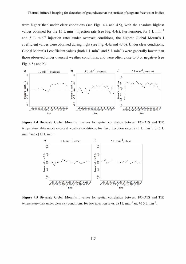
Thermal infrared imaging for detection of groundwater at the surface of stagnant freshwater bodies
115
were higher than under clear conditions (see Figs. 4.4 and 4.5), with the absolute highest
values obtained for the 15 L min−1 injection rate (see Fig. 4.4c). Furthermore, for 1 L min−1
and 5 L min−1 injection rates under overcast conditions, the highest Global Moran’s I
coefficient values were obtained during night (see Fig. 4.4a and 4.4b). Under clear conditions,
Global Moran’s I coefficient values (both 1 L min−1 and 5 L min−1) were generally lower than
those observed under overcast weather conditions, and were often close to 0 or negative (see
Fig. 4.5a and b).
Figure 4.4 Bivariate Global Moran’s I values for spatial correlation between FO-DTS and TIR
temperature data under overcast weather conditions, for three injection rates: a) 1 L min−1, b) 5 L
min−1 and c) 15 L min−1.
Figure 4.5 Bivariate Global Moran’s I values for spatial correlation between FO-DTS and TIR
temperature data under clear sky conditions, for two injection rates: a) 1 L min−1 and b) 5 L min−1.

116
4.4 Discussion
4.4.1 Comparison of TIR temperature data with FO-DTS temperature data
Visual and quantitative comparison of the TIR temperatures with FO-DTS data demonstrated
that best matches occurred during overcast weather conditions than during clear sky
conditions, during night than during day and at higher injection rates than at lower injection
rates (Figs. 4.2–4.5). FO-DTS observations provided a spatially-explicit validation for the
patterns observed in the TIR images for a range of different discharge rates, weather
conditions and points along the diurnal cycle. The FO-DTS setup allowed for the
differentiation of thermal anomalies related to groundwater upwelling from thermal anomalies
present within the TIR images which were related to other factors (e.g. reflections from
vegetation). The use of near-surface mounted FO-DTS to validate TIR in this manner is
novel, as the majority of other studies incorporating FO-DTS measurements and TIR use FO-
DTS installed at the sediment-water interface (e.g. Lewandowski et al., 2013). In such studies,
comparison of TIR images with FO-DTS temperature data is problematic because: a) depth-
dependent mixing may fundamentally alter the thermal patterns received by the FO-DTS in
comparison with TIR and b) the warming effect of incident radiation at the air water interface
(e.g. Benyahya et al., 2012; Marruedo Arricibita et al., 2018; Ouellet et al., 2014) may not be
recorded by the bed-mounted FO-DTS. Our experimental setup provides a partial resolution
of this problem, allowing for more direct comparison of the two techniques.
4.4.2 Influence of discharge rates, weather conditions and the diurnal cycle
Simulated discharge rates
Higher simulated discharge rates increased the ability of TIR to detect warm upwelling at the
surface. The simulated discharge rates in the present study (1–15 L min−1
) are at the higher
end of LGD rates reported worldwide (e.g. 745 cm day−1
=5.2 L m−2
min−1
reported in
Rosenberry et al., 2015). Examples of similarly high discrete LGD are found in Karst aquifers
or in humic lakes with macropore groundwater discharge, occasionally exceeding 15 L min−1
(e.g. Norrström and Jacks, 1996). Nevertheless, we appreciate that the simulated discharge
rates are much higher than those typically observed in nature. Our values were chosen with a
view to understanding the upper and lower limits of detectability using TIR in high discrete
LGD environments under a best-case scenario. Thus, we do not recommend the extrapolation
of our results or the use of TIR for studying LGD at the lower end of rates reported in the
literature (e.g. 0.005–124.1 cm day−
; 1
Rosenberry et al., 2015).

Thermal infrared imaging for detection of groundwater at the surface of stagnant freshwater bodies
117
Influence of weather conditions
The present study builds on the mechanistic findings of Marruedo Arricibita et al. (2018)
whereby the propagation of relatively warm water from the sediment to the air-water interface
was tracked by several layers of FO-DTS cable in the water column. Marruedo Arricibita et
al. (2018) showed that the propagation of relatively warm water heat signal from the sediment
to the air-water interface was mainly influenced by the diurnal cycle of net radiation (Rn) and
cloud cover, due to the role of Rn in controlling heat gains and losses at the water surface.
These findings also have implications for the TIR results. During daytime, Rn values were
higher under clear skies than under overcast weather conditions, due to increased incident
shortwave radiation. This means that the water surface heated up more than under overcast
weather conditions, rendering the signal from the warm water injection (at the base of the
mesocosm) difficult to observe with TIR (because of the very small resultant temperature
difference between the simulated upwelling and the ambient mesocosm surface temperature).
On the contrary, during night-time, a greater amount of net radiation (Rn) was lost during
clear sky conditions than under overcast conditions (Marruedo Arricibita et al., 2018). While
this increased heat loss explains why the FO-DTS data was not able to properly characterise
upwelling (due to rapid dissipation of heat energy at the surface), it does not explain why the
TIR images were not readily able to detect the upwelling, as it is this very loss of radiation
which is measured by the thermal camera. Instead, we hypothesise that the formation of a
(shallow) inverted thermocline resulting from the high surface energy loss may have
prevented warm water from reaching the surface prior to mixing, possibly explaining the lack
of an observable plume extent in the TIR images.
The TIR sensor measures longwave radiation that is emitted and reflected from the water
surface. This means that thermal images obtained from TIR cameras contain information on
both water surface temperature and reflections from surrounding vegetation (in this case, tree
cover next to the mesocosm) or cloud cover (Anderson and Wilson, 1984; Handcock et al.,
2012; Schott, 1994; Torgersen et al., 2001). In addition, the sensor in the TIR camera detects
radiation emitted from the upper 0.1 mm of the water surface (Torgersen et al., 2001),
whereas the FO-DTS measured true kinetic temperature at 2 cm below the water surface. As a
consequence, FO-DTS temperature measurements, unlike the TIR data, were not affected by
radiation emitted by surrounding vegetation or clouds.
Under clear sky conditions, the TIR imagery incorporated artefacts generated from longwave
reflections of tree cover. These artefacts caused temperature variations at the water surface
118
and made it extremely difficult to discriminate the extent of the thermal plume associated with
the warm water injection. The match with the FO-DTS data (which were not influenced by
vegetation reflections) was therefore poor. Conversely, under overcast weather conditions, it
was possible to discriminate the extent of the thermal plume associated with the warm water
injection in the TIR image. We provide two possible explanations for this phenomenon. First,
during overcast conditions, the TIR imagery incorporated longwave reflections not only from
vegetation, but also from cloud cover. As a consequence, most reflections from vegetation
were masked by bulk reflections of clouds, which provided a relatively uniform background
in the TIR image. The thermal plume from the warm water injection into the mesocosm was
thus visible against the uniform background, providing an improved degree of similarity
between the FO-DTS and TIR data. Second, the decrease in solar radiation under overcast
conditions meant that resulting longwave emissions from trees were also diminished, reducing
the magnitude of reflections from tree cover.
Influence of the diurnal cycle
Although overcast conditions aided detection of the warm water injection during both day and
night, it was generally easier to detect the thermal plume during the night, when longwave
reflections from trees beside the mesocosm were minimized. Longwave emissions from
vegetation are lower at night because vegetation temperature is generally reduced in
comparison to daylight conditions (owing to a lack of incident shortwave radiation at night).
This resulted in substantially weaker longwave emissions from vegetation to the water
surface, eliminating vegetation reflections in the TIR images and further aiding discrimination
of the thermal plume.
4.4.3 Experimental shortcomings and future improvements
The present experiment was conducted in a semi-controlled environment (a mesocosm with
simulated groundwater discharge) in order to decrease the number of external influences (e.g.
turbulence from waves, vegetation in the water column) on the ability of TIR to detect the
warm water injection. This experimental setup allowed us to better isolate and investigate the
influence of weather conditions (clear vs overcast) and the diurnal cycle (day vs night), which
might otherwise be obscured by other external phenomena. Our results could be applied or
extrapolated to shallow lakes up to 1 m deep, or shallow littoral environments, provided wind
velocities and mixing were sufficiently similar. However, we acknowledge: (i) that in natural
environments, the ability of TIR to detect warm groundwater upwelling in winter is also
influenced by a range of other factors and; (ii) the limited number of parameters (discharge

Thermal infrared imaging for detection of groundwater at the surface of stagnant freshwater bodies
119
rates, weather conditions and diurnal cycle) included in this study. This experiment is a first
attempt to understand under which conditions ground-based TIR remote sensing is a suitable
method to detect discrete LGD at the water surface of slow flowing freshwater bodies such as
lakes, ponds or reservoirs, in winter. Therefore, we advocate further research that will build
upon the lessons learned from the results and conclusions presented in this paper, through the
use of more detailed experimental designs capable of examining a larger variation of
parameters (e.g. surface water depth, angle of the TIR camera or the range of ΔT between
surface water and groundwater) or future measurements in natural conditions (conducted from
the shores of lakes).
4.4.4 Implications of results for TIR based monitoring of groundwater upwelling
Our study emphasizes the importance of considering the influences of weather conditions
(clear vs overcast) and the diurnal cycle (day vs night) on TIR-based detection of LGD in
slow flowing freshwater. The emphasis on the relevance of weather conditions and the diurnal
cycle is in agreement with other recent investigations which also highlighted similar findings
(e.g. bedrock groundwater seepage detection; Mundy et al., 2017; TIR imaging of high
altitude alpine environments; Aubry-Wake et al., 2015). Indeed, in a study designed to assess
the influence of air temperature and solar radiation on ground-based TIR measurements of
groundwater seepage from bedrock, Mundy et al. (2017) specifically recommended that TIR
temperature measurements should be carried out when solar radiation is not present (during
night) and in stable weather conditions. This finding supports our results and highlights the
importance of conducting monitoring: i) at night and; ii) under overcast weather conditions.
Thus, while close-range TIR techniques can constitute an effective tool for monitoring
groundwater upwelling, their efficacy depends upon a wide range of environmental factors.
Care must therefore be taken when performing similar work to control for the factors detailed
in this paper to ensure optimal monitoring results.
We also note that our TIR imagery required post-processing to account for the effects of
vignetting. Vignetting results in a circular gradient of decreasing image brightness from the
centre of the image to its edges (Gupta, 2018; Lelong et al., 2008). Although commonly
associated with optical remote sensing (e.g. Kordecki et al., 2016; Meng et al., 2015),
vignetting is also known to impact TIR images in a similar fashion (e.g. Hook et al., 2005;
Meier et al., 2011) resulting in generally ‘cooler’ temperatures towards the edges of TIR
images. This effect is particularly pronounced with wide angle lenses (Goldman, 2010;
120
Kelcey and Lucieer, 2012), such as the 12.5 mm (65° × 51° field-of-view) model used in our
study. While such vignetting is therefore unlikely to present challenges for airborne TIR
which benefit from the ability to use narrower field-of-view (FOV) lenses due to increased
sensor to object distances, the use of wide FOV lenses is often a necessity in ground-based
TIR studies in order to acquire imagery of a given study area in its entirety. Future ground-
based studies of discrete LGD should therefore be aware of the potential for temperature bias
resulting from the use of wide-angle lenses; such studies may therefore require the application
of similar post-processing methodologies to account for this.
4.5 Conclusions
The manifestation of warm water upwelling at the surface of a mesocosm was monitored
using TIR and compared to FO-DTS temperature observations for a range of different
injection rates. Results show that the diurnal cycle of incoming net radiation as well as
weather conditions (clear versus overcast skies) had a substantial effect on the ability of TIR
to accurately detect simulated warm water upwelling (in comparison to FO-DTS records).
While simulated warm water discharges were generally well detected during overcast
conditions and at night, TIR was less able to replicate FO-DTS observations during day and
under clear sky conditions. These findings have important implications for the use of TIR
imaging to detect discrete LGD at the water surface of slow flowing freshwater bodies in
winter.
Thermal infrared imaging for detection of groundwater at the surface of stagnant freshwater bodies
121
Acknowledgments and Data
Funding: This work was supported by the European Union’s Seventh Framework programme
for research; technological development and demonstration [grant number 60715]:
Ecohydrological Interfaces as Critical Hotspots for Transformations of Ecosystem Exchange
Fluxes (INTERFACES).
The data supporting the conclusions can be obtained in the results section, figures and
references.
Special thanks to Franziska Pöschke, Karin Meinikmann, Hauke Dämpfling and Anne
Mehrtens for their technical and moral support.
Finally, we would like to thank the two anonymous reviewers and the editor Tim R. McVicar
for the detailed and helpful reviews provided.

122
References
Allan, R.G., Pereira, L., Raes, D., Smith, M., 1998. Crop evapotranspiration-Guidelines for
computing crop water requirements-FAO Irrigation and drainage paper 56.
Anderson, D.M., Glibert, P.M., Burkholder, J.M., 2002. Harmful algal blooms and
eutrophication: nutrient sources, composition, and consequences. Estuaries 25, 704–726.
http://dx.doi.org/10.1007/BF02804901.
Anderson, J.M., Wilson, S.B., 1984. Review Article. The physical basis of current infrared
remote-sensing techniques and the interpretation of data from aerial surveys. Int. J.
Remote Sens. 1–18. http://dx.doi.org/10.1080/01431168408948786.
Anselin, L., 1995. Local indicators of spatial association-LISA. Geogr. Anal. 27, 93–115.
http://dx.doi.org/10.1111/j.1538-4632.1995.tb00338.x.
Anselin, L., Syabri, I., Smirnov, O., 2002. Visualizing Multivariate Spatial Correlation with
Dynamically Linked Windows. in: Anselin, L., Rey, S. (Eds.), New Tools for Spatial Data
Analysis: Proceedings of the Specialist Meeting. Santa Barbara.
Aubry-Wake, C., Baraer, M., McKenzie, J.M., Mark, B.G., Wigmore, O., Hellström, R.,
Lautz, L., Somers, L., 2015. Measuring glacier surface temperatures with groundbased
thermal infrared imaging. Geophys. Res. Lett. 42, 8489–8497. http://dx.doi.
org/10.1002/2015GL065321.
Baker, B.H., Martinovic-Weigelt, D., Ferrey, M., Barber, L.B., Writer, J.H., Rosenberry,
D.O., Kiesling, R.L., Lundy, J.R., Schoenfuss, H.L., 2014. Identifying non-point sources of
endocrine active compounds and their biological impacts in freshwater lakes. Arch.
Environ. Contam. Toxicol. 67, 374–388. http://dx.doi.org/10.1007/ s00244-014-0052-4.
Benyahya, L., Caissie, D., Satish, M.G., El-Jabi, N., 2012. Long-wave radiation and heat flux
estimates within a small tributary in Catamaran Brook (New Brunswick, Canada), 484,
475–484. doi: 10.1002/hyp.8141.
Boulton, A.J., Findlay, S., Marmonier, P., Stanley, E.H., Boulton, A.J., Findlay, S.,
Marmonier, P., Stanley, E.H., Valett, H.M., 1998. The Functional Significance of the
Hyporheic Zone in Streams and Rivers Maurice Valett Source : Annual Review of Ecology
and Systematics, Vol. 29 (1998), pp. 59–81 Published by : Annual Reviews Stable URL :
http://www.jstor.org/stable/221702 REFERENC 29, 59–81.
Brabrand, Å., Koestler, A.G., Borgstrøm, R., 2002. Lake spawning of brown trout related to
groundwater influx. J. Fish Biol. 60, 751–763. http://dx.doi.org/10.1006/jfbi. 2002.1901.
Thermal infrared imaging for detection of groundwater at the surface of stagnant freshwater bodies
123
Briggs, M.A., Hare, D.K., Boutt, D.F., Davenport, G., Lane, J.W., 2016. Thermal infrared
video details multiscale groundwater discharge to surface water through macropores and
peat pipes. Hydrol. Process. 30, 2510–2511. http://dx.doi.org/10.1002/hyp. 10722.
Briggs, M.A., Voytek, E.B., Day-Lewis, F.D., Rosenberry, D.O., Lane, J.W., 2013.
Understanding water column and streambed thermal refugia for endangered mussels in the
Delaware River. Environ. Sci. Technol. 47, 11423–11431. http://dx.doi.org/
10.1021/es4018893.
Burnett, W.C., Aggarwal, P.K., Aureli, A., Bokuniewicz, H., Cable, J.E., Charette, M.A.,
Kontar, E., Krupa, S., Kulkarni, K.M., Loveless, A., Moore, W.S., Oberdorfer, J.A.,
Oliveira, J., Ozyurt, N., Povinec, P., Privitera, A.M.G., Rajar, R., Ramessur, R.T., Scholten,
J., Stieglitz, T., Taniguchi, M., Turner, J.V., 2006. Quantifying submarine groundwater
discharge in the coastal zone via multiple methods. Sci. Total Environ.
367, 498–543. http://dx.doi.org/10.1016/j.scitotenv.2006.05.009.
Burnett, W.C., Bokuniewicz, H., Huettel, M., Moore, W.S., Taniguchi, M., 2003.
Groundwater and pore water inputs to the coastal zone. Biogeochemistry 66, 3–33.
http://dx.doi.org/10.1023/B:BIOG.0000006066.21240.53.
Danielescu, S., MacQuarrie, K.T.B., 2011. Nitrogen loadings to two small estuaries, Prince
Edward Island, Canada: a 2-year investigation of precipitation, surface water and
groundwater contributions. Hydrol. Process. 957, 945–957. http://dx.doi.org/10.
1002/hyp.7881.
Danielescu, S., MacQuarrie, K.T.B., Faux, R.N., 2009. The integration of thermal infrared
imaging, discharge measurements and numerical simulation to quantify the relative
contributions of freshwater inflows to small estuaries in Atlantic Canada. Hydrol.
Process. 23, 2847–2859. http://dx.doi.org/10.1002/hyp.7383.
Davies, A.G., Calkins, J., Scharenbroich, L., Vaughan, R.G., Wright, R., Kyle, P., Castańo,
R., Chien, S., Tran, D., 2008. Multi-instrument remote and in situ observations of the
Erebus Volcano (Antarctica) lava lake in 2005: a comparison with the Pele lava lake on the
jovian moon Io. J. Volcanol. Geotherm. Res. 177, 705–724. http://dx.doi.org/
10.1016/j.jvolgeores.2008.02.010.
Dugdale, S.J., 2016. A practitioner’s guide to thermal infrared remote sensing of rivers and
streams: recent advances, precautions and considerations. Wiley Interdiscip. Rev. Water 3,
251–268. http://dx.doi.org/10.1002/wat2.1135.

124
Dugdale, S.J., Bergeron, N.E., St-Hilaire, A., 2015. Spatial distribution of thermal refuges
analysed in relation to riverscape hydromorphology using airborne thermal infrared
imagery. Remote Sens. Environ. 160, 43–55. http://dx.doi.org/10.1016/j.rse.2014.
12.021.
Frisbee, M.D., Shope, C.L., Briggs, M., Boutt, D.F., 2016. Field methods for the evaluation of
groundwater and surface-water interactions. In: Cushman, J.H., Tartakovski, D.M. (Eds.),
The Handbook of Groundwater Engineering. CRC Press.
Goldman, D.B., 2010. Vignette and exposure calibration and compensation. IEEE Trans.
Pattern Anal. Mach. Intell. 32, 2276–2288. http://dx.doi.org/10.1109/TPAMI. 2010.55.
Gupta, R.P., 2018. Image Quality and Principles of Interpretation. In: Remote Sensing
Geology. Springer, Berlin, Heidelberg, pp. 107–114. http://dx.doi.org/10.1007/9783-662-
55876-8_9.
Handcock, R.N., Torgersen, C.E., Cherkauer, K.A., Gillespie, A.R., Tockner, K., Faux, R.N.,
Tan, J., 2012. Thermal infrared remote sensing of water temperature in riverine landscapes.
Fluv. Remote Sens. Sci. Manag. 85–113. http://dx.doi.org/10.1002/ 9781119940791.ch5.
Hare, D.K., Briggs, M.A., Rosenberry, D.O., Boutt, D.F., Lane, J.W., 2015. A comparison of
thermal infrared to fiber-optic distributed temperature sensing for evaluation of
groundwater discharge to surface water. J. Hydrol. 530, 153–166. http://dx.doi.org/
10.1016/j.jhydrol.2015.09.059.
Hayashi, M., Rosenberry, D., 2002. Effects of ground water exchange on the hydrology and
ecology of surface water. Ground Water 40, 309–316.
Hook, S.J., Clodius, W.B., Balick, L., Alley, R.E., Abtahi, A., Richards, R.C., Schladow,
S.G., 2005. In-flight validation of mid- and thermal infrared data from the Multispectral
Thermal Imager (MTI) using an automated high-altitude validation site at Lake Tahoe
CA/NV, USA. IEEE Trans. Geosci. Remote Sens. 43, 1991–1999. http://
dx.doi.org/10.1109/TGRS.2005.853191.
Hu, C., Muller-karger, F.E., Swarzenski, P.W., 2006. Hurricanes, submarine groundwater
discharge, and Florida ’ s red tides. Geophys. Res. Lett. 33, 1–5. http://dx.doi.org/10.
1029/2005GL025449.
Johnson, A.G., Glenn, C.R., Burnett, W.C., Peterson, R.N., Lucey, P.G., 2008. Aerial infrared
imaging reveals large nutrient-rich groundwater inputs to the ocean. Geophys. Res. Lett. 35,
1–6. http://dx.doi.org/10.1029/2008GL034574.
Kelcey, J., Lucieer, A., 2012. Sensor correction of a 6-band multispectral imaging sensor for
UAV remote sensing. Remote Sens. 4, 1462–1493. http://dx.doi.org/10.3390/ rs4051462.

Thermal infrared imaging for detection of groundwater at the surface of stagnant freshwater bodies
125
Kordecki, A., Palus, H., Bal, A., 2016. Practical vignetting correction method for digital
camera with measurement of surface luminance distribution. Signal Image Video Process.
10, 1417–1424. http://dx.doi.org/10.1007/s11760-016-0941-2.
Krause, S., Blume, T., 2013. Impact of seasonal variability and monitoring mode on the
adequacy of fiber-optic distributed temperature sensing at aquifer-river interfaces.
Water Resour. Res. 49, 2408–2423. http://dx.doi.org/10.1002/wrcr.20232.
Lee, E., Kang, K., Hyun, S.P., Lee, K.-Y., Yoon, H., Kim, S.H., Kim, Y., Xu, Z., Kim, D.,
Koh, D.-C., Ha, K., 2016. Submarine groundwater discharge revealed by aerial thermal
infrared imagery: a case study on Jeju Island, Korea. Hydrol. Process. 3506, 3494–3506.
http://dx.doi.org/10.1002/hyp.10868.
Lee, Y., Kim, G., 2007. Linking groundwater-borne nutrients and dinoflagellate red-tide
outbreaks in the southern sea of Korea using a Ra tracer. Estuar. Coast. Shelf Sci. 71, 309–
317. http://dx.doi.org/10.1016/j.ecss.2006.08.004.
Lega, M., Napoli, R.M.a., 2010. Aerial infrared thermography in the surface waters
contamination monitoring. Desalin. Water Treat. 23, 141–151. http://dx.doi.org/10.
5004/dwt.2010.1988.
Lelong, C.C.D., Burger, P., Jubelin, G., Roux, B., Labbé, S., Baret, F., 2008. Assessment of
unmanned aerial vehicles imagery for quantitative monitoring of wheat crop in small plots.
Sensors 8, 3557–3585. http://dx.doi.org/10.3390/s8053557.
Lewandowski, J., Meinikmann, K., Ruhtz, T., Pöschke, F., Kirillin, G., 2013. Localization of
lacustrine groundwater discharge (LGD) by airborne measurement of thermal infrared
radiation. Remote Sens. Environ. 138, 119–125. http://dx.doi.org/10.1016/j.
rse.2013.07.005.
Marruedo Arricibita, A.I., Krause, S., Gomez-Velez, J., Hannah, D.M., Lewandowski, J.,
2018. Mesocosm experiments identifying hotspots of groundwater upwelling in a water
column by fibre optic distributed temperature sensing. Hydrol. Process. 32, 185–199.
http://dx.doi.org/10.1002/hyp.11403.
Meier, F., Scherer, D., Richters, J., Christen, A., 2011. Atmospheric correction of thermal
infrared imagery of the 3-D urban environment acquired in oblique viewing geometry.
Atmos. Meas. Tech. 4, 909–922. http://dx.doi.org/10.5194/amt-4-909-2011.
Meinikmann, K., Lewandowski, J., Nützmann, G., 2013. Lacustrine groundwater discharge:
combined determination of volumes and spatial patterns. J. Hydrol. 502, 202–211.
http://dx.doi.org/10.1016/j.jhydrol.2013.08.021.

126
Meng, H., Guan, W., Liu, C., Wu, Q., 2015. Algorithm research of vignetting distortion
correction based on near-infrared CCD thermometer, in: Design, Manufacturing and
Mechatronics. WORLD SCIENTIFIC, pp. 1290–1298. doi:10.1142/9789814730518_
0151.
Mundy, E., Gleeson, T., Roberts, M., Baraer, M., Mckenzie, J.M., 2017. Thermal imagery of
groundwater seeps: possibilities and limitations. Groundwater. http://dx.doi.org/
10.1111/gwat.12451.
Nakayama, T., Watanabe, M., 2008. Missing role of groundwater in water and nutrient cycles
in the shallow eutrophic Lake Kasumigaura, Japan. Hydrol. Process. 22, 1150–1172.
http://dx.doi.org/10.1002/hyp.6684.
Neale, C.M.U., Jaworowski, C., Heasler, H., Sivarajan, S., Masih, A., 2016. Hydrothermal
monitoring in Yellowstone National Park using airborne thermal infrared remote sensing.
Remote Sens. Environ. 184, 628–644. http://dx.doi.org/10.1016/j.rse.2016.
04.016.
Norrström, A.C., Jacks, G., 1996. Water pathways and chemistry at the groundwater/ surface
water interface to Lake Skjervatjern, Norway. Water Resour. Res. 32, 2221–2229 0043-
1397/96/96WR-00802.
Ouellet, V., Secretan, Y., St-Hilaire, A., Morin, J., 2014. Water temperature modelling in a
controlled environment: comparative study of heat budget equations. Hydrol.
Process. 28, 279–292. http://dx.doi.org/10.1002/hyp.9571.
Röper, T., Greskowiak, J., Massmann, G., 2014. Detecting small groundwater discharge
springs using handheld thermal infrared imagery. Groundwater 52, 936–942. http://
dx.doi.org/10.1111/gwat.12145.
Rosenberry, D.O., Lewandowski, J., Meinikmann, K., Nützmann, G., 2015. Groundwater –
the disregarded component in lake water and nutrient budgets. Part 1: effects of
groundwater on hydrology. Hydrol. Process. 29, 2895–2921. http://dx.doi.org/10.
1002/hyp.10403.
Schott, J.R., 1994. Thermal infrared calibration of aerial and satellite images over land, in:
geoscience and remote sensing symposium. IEEE, Pasadena, CA, pp. 1–4. doi: 10.
1109/IGARSS.1994.399083.
Schuetz, T., Weiler, M., 2011. Quantification of localized groundwater inflow into streams
using ground-based infrared thermography. Geophys. Res. Lett. 38, 1–5.
http://dx.doi.org/10.1029/2010GL046198.

Thermal infrared imaging for detection of groundwater at the surface of stagnant freshwater bodies
127
Schuetz, T., Weiler, M., Lange, J., Stoelzle, M., 2012. Two-dimensional assessment of solute
transport in shallow waters with thermal imaging and heated water. Adv.
Water Resour. 43, 67–75. http://dx.doi.org/10.1016/j.advwatres.2012.03.013.
Shaw, R.D., Shaw, J.F.H., Fricker, H., Prepas, E.E., 1990. An integrated approach to quantify
groundwater transport of phosphorus to Narrow Lake. Alberta 35, 870–886. Sobrino, J.A., Del
Frate, F., Drusch, M., Jiménez-Muñoz, J.C., Manunta, P., Regan, A., 2016. Review of thermal
infrared applications and requirements for future high-resolution sensors. IEEE Trans. Geosci.
Remote Sens. 54, 2963–2972. http://dx.doi. org/10.1109/TGRS.2015.2509179.
Tamborski, J.J., Rogers, A.D., Bokuniewicz, H.J., Cochran, J.K., Young, C.R., 2015.
Identification and quantification of diffuse fresh submarine groundwater discharge via
airborne thermal infrared remote sensing. Remote Sens. Environ. 171, 202–217.
http://dx.doi.org/10.1016/j.rse.2015.10.010.
Taniguchi, M., Burnett, W.C., Cable, J.E., Turner, J.V., 2002. Investigation of submarine
groundwater discharge. Hydrol. Process. 2129, 2115–2129. http://dx.doi.org/10.
1002/hyp.1145.
Tcherepanov, E.N., Zlotnik, V.a., Henebry, G.M., 2005. Using Landsat thermal imagery and
GIS for identification of groundwater discharge into shallow groundwater dominated lakes.
Int. J. Remote Sens. 26, 3649–3661. http://dx.doi.org/10.1080/ 01431160500177315.
Tempelhahn, A., Budzier, H., Krause, V., Gerlach, G., 2016. Shutter-less calibration of
uncooled infrared cameras. J. Sensors Sens. Syst. 5, 9–16. http://dx.doi.org/10.5194/ jsss-5-
9-2016.
Tempelhahn, A., Budzier, H., Krause, V., Gerlach, G., 2015. Development of a shutterless
calibration process for microbolometer-based infrared measurement systems. ejournal
Nonde- structive. Test 20. http://dx.doi.org/10.21611/qirt.2014.060.
Torgersen, C.E., Faux, R.N., McIntosh, B.A., Poage, N.J., Norton, D.J., 2001. Airborne
thermal remote sensing for water temperature assessment in rivers and streams. Remote
Sens. Environ. 76, 386–398. http://dx.doi.org/10.1016/S0034-4257(01) 00186-9.
Wang, X., Wang, X., Fan, J., Wen, S., Zhao, J., Su, X., 2016. Comparison of different spatial
resolution thermal infrared data in monitoring thermal plume from the Hongyanhe nuclear
power plant. 2016 IEEE Int. Geosci. Remote Sens. Symp.
4649–4652. doi: 10.1109/IGARSS.2016.7730213.
Warren, D.R., Sebestyen, S.D., Josephson, D.C., Lepak, J.M., Kraft, C.E., 2005. Acidic
groundwater discharge and in situ egg survival in redds of lake-spawning brook trout.

128
Trans. Am. Fish. Soc. 134, 1193–1201. http://dx.doi.org/10.1577/T04-180.1.
Wawrzyniak, V., Piégay, H., Allemand, P., Vaudor, L., Goma, R., Grandjean, P., 2016.
Effects of geomorphology and groundwater level on the spatio-temporal variability of
riverine cold water patches assessed using thermal infrared (TIR) remote sensing. Remote
Sens. Environ. 175, 337–348. http://dx.doi.org/10.1016/j.rse.2015.12.050.
Wirth, L., Rosenberger, A., Prakash, A., Gens, R., Margraf, J.F., Hamazak, T., 2012. A
remote-sensing, gis-based approach to identify, characterize, and model spawning habitat
for fall-run chum salmon in a sub-arctic, glacially fed River. Trans. Am. Fish. Soc. 141,
1349–1363. http://dx.doi.org/10.1080/00028487.2012.692348.
Zuo, C., Chen, Q., Gu, G., Sui, X., 2011. Scene-based non-uniformity correction algorithm
based on interframe registration. J. Opt. Soc. Am. A 28 (6), 1164. http://dx.doi.org/
10.1364/JOSAA.28.001164.

Thermal infrared imaging for detection of groundwater at the surface of stagnant freshwater bodies
129
130
5 Synopsis
5.1 Summary of results
The positive buoyancy of relatively warm water imported by (simulated) LGD into
shallow water bodies (e.g. the mesocosm) allows detection of LGD at the water
surface-atmosphere interface by FO-DTS. Injection of warm water was conducted
with different rates under different weather conditions (clear vs. overcast) over the
entire diurnal cycle. This resulted in different upwelling patterns across the water
column were described from the sediment-water interface through the water column to
the water surface-atmosphere interface. Upwelling signals at the water surface were
identified at all applied injection rates: 1 L min-1
, 5 L min-1
and 15 L min-1
. However,
detectability of simulated LGD at the water surface-atmosphere interface was mainly
determined by the diurnal cycle of the net radiation balance (Rn) and the cloud cover.
Detection of simulated LGD at the water surface-atmosphere interfaces was best under
overcast conditions and during the night (Chapter 3 and Figure 3.3).
TIR can detect upwelling at the water surface. The diurnal cycle of incoming
shortwave radiation as well as weather conditions (clear vs. overcast) have a
substantial effect on the ability of TIR to accurately detect simulated warm water
upwelling (in comparison to FO-DTS measurements). While simulated LGD was
generally well-detected during overcast conditions and at night, TIR was less able to
replicate FO-DTS observations during day and under clear sky conditions (Chapter 4,
Figures 4.2 and 4.3).
The HPD based approach is helpful to distinguish the overlapping impacts of heat
transport processes across spatial and temporal scales. Heat fluxes related to simulated
LGD and heat fluxes from the atmosphere (e.g. incident shortwave radiation) overlap
across spatial and temporal scales. The detection of heat as a tracer for LGD depends
on whether the heat signal related to LGD is dominant or overshadowed by heat fluxes
coming from the atmosphere (Chapter 2).
5.2 Discussion
5.2.1 Impacts of diurnal cycle of net radiation and cloud cover on tracing of
LGD
In the present PhD thesis, hydrometeorological parameters are identified as main controlling
factors for detection of GW-SW interactions (in this case, LGD) at the water surface of
stagnant water bodies such as lakes (research goal n°3, chapter 1.3). The strength of the heat
Synopsis
131
or temperature signal that solely belongs to the simulated warm LGD in the water column and
at the water surface-atmosphere interface was strongly controlled by weather conditions (clear
sky and overcast sky) and the diurnal cycle of the net radiation (Figures 3.3, 3.7 and 3.9). For
instance, when simulating warm LGD at a rate of 1 L min-1
, the heat signal of the simulated
warm LGD could be distinguished across the entire extent of the water column and the water
surface but only under overcast weather conditions (Chapter 3, Figure 3.3 d). On the contrary,
the heat signal of the simulated warm LGD could not be distinguished (during day) or did not
reach the water surface (during night) under clear sky conditions (Chapter 3, Figure 3.3 a). In
addition, calculated net heat fluxes across the water surface were stronger during clear sky
day and more negative during clear sky night than during overcast day and night respectively
(Chapter 3, Figure 3.8 a). This means that more heat was gained during the day or lost during
the night across the water surface-atmosphere interface under clear sky conditions.
A more in-depth analysis revealed that the main component of the net heat fluxes across the
water surface was the net radiation which is the sum of the net shortwave and the net
longwave radiation (Chapter 3, Figure 3.8). Therefore, the diurnal cycle of the net radiation
balance controlled the strength of the heat fluxes across the water surface and in consequence,
the gains and losses of heat across the water surface. For this reason, during day under clear
sky conditions, the warming effect of incident shortwave radiation at the water surface and
some cm below the water surface prevented a differentiation of the heat signals of the
simulated warm LGD and the radiation. During night under clear sky conditions, the heat
signal of the simulated warm LGD was lost due to the strong cooling effect of the net
longwave radiation across the water surface.
Finally, the cloud cover (clear sky vs. overcast sky) played an important role for the strength
of the heat signal caused by simulated warm LGD. Cloud cover is an important controller of
the diurnal cycle of the net radiation balance (Dai and Trenberth, 1999; Betts, 2003, 2015;
Betts et al., 2013) 1) by diminishing the incident shortwave radiation at the water surface and
2) by diminishing the cooling due to net longwave radiation from the water surface. This
means that the heat gains and losses across the water surface under overcast conditions are
smaller than under clear sky conditions. Therefore, during day under overcast conditions the
heat signal related to the simulated warm LGD was discernible across the water column and
at the water surface. During night under overcast conditions, the cooling effect of net
longwave radiation at the water surface was weaker than under clear sky conditions,

132
preventing the loss of the heat signal related to the simulated warm LGD at the water surface
as occurred under clear sky conditions.
5.2.2 FO-DTS for monitoring LGD in lakes
Most research on GW-SW interactions with FO-DTS is done in streams (Lowry et al., 2007;
Slater et al., 2010; Krause et al., 2012; Briggs et al., 2013, 2016a; Mamer and Lowry, 2013;
Birkham et al., 2014; González-pinzón et al., 2015; Rosenberry et al., 2016) while research
on lakes is not as common (Blume et al., 2013; Sebok et al., 2013; Liu et al., 2015; Tristram
et al., 2015). Typically, the FO-DTS cable is deployed directly on the sediment bed or buried
few cm in the sediment (Blume et al., 2013; Tristram et al., 2015). There are also few studies
where the DTS cable was wrapped around tubes and inserted in the sediment to get a high
resolution depth profile (Vogt et al., 2010). To the best of my knowledge there is only one
other study in which DTS was used to trace the heat signal of LGD across the water column.
Sebok et al. (2013) deployed the FO-DTS at three different depths in the water column of
Lake Væng close to the shore of the lake and at three different distances from the shore of the
lake. Influence of solar radiation on monitored water temperatures by FO-DTS was
mentioned as a relevant factor affecting the detection of LGD across the water column and the
water surface-atmosphere interface during the spring and summer months. Only night
measurements reliably detected LGD for periods with strong solar radiation. However, in
Sebok et al. (2013) the influence of solar radiation during winter conditions was neglected.
Finally Sebok et al. (2013) concluded that the positive buoyancy of the LGD was responsible
for the lack of ice cover at those specific water surface areas recommending more elaborate
multilevel FO-DTS setups in order to further understand the development of the thermal
plumes related to LGD in three dimensions. The three dimensional and more elaborated FO-
DTS setup of the present PhD thesis allowed describing interactions between simulated GW
discharge, upwelling warm water and cold SW in terms of spatial and temporal distribution of
temperature through the water column (research goal n°2, chapter 1.3) at different weather
conditions and over the entire diurnal cycle (Chapter 3 and Figure 3.3). The different warm
water upwelling patterns monitored by the FO-DTS setup, allowed considering possible
connections between the monitored spatial patterns of the heat signal and the different
weather conditions and the diurnal cycle (addressed in chapter 5.2.1). Thus, FO-DTS is a
useful method for spatial pattern characterization of warm water upwelling in the water
column and for supporting other methods (e.g. TIR) to identify hotspots of GW discharge at
different interfaces such as at the water surface-atmosphere interface. Some other researches
(e.g. Blume et al., 2013) successfully used as well FO-DTS in combination with other
Synopsis
133
methods for 2 dimensional spatial pattern identification of LGD at the sediment-water
interface. In addition, in most of the studies (Krause et al., 2012; Sebok et al., 2015) the main
focus is on the horizontal spatial pattern characterization at the sediment surface or at the
water surface in order to get more insights about LGD and to detected hotspots of GW
discharge. Thus, generally the FO-DTS is not setup across the water column. However,
vertical pattern characterization across the water column of simulated LGD allowed
understanding the mechanism of the upwelling process of warm GW and how the heat signal
propagated across the water column. Thus, 2 and 3 dimensional FO-DTS setups seem to
improve the mechanistic understanding of LGD in terms of temperature spatial patterns at
different interfaces (sediment-water or water surface-atmosphere) and across the water
column.
Finally, since TIR imaging is the most appropriate method for monitoring water temperature
at the water surface, FO-DTS is a reliable method for ground truthing TIR data monitored at
the water surface (see Chapter 4).
5.2.3 TIR imaging for detection of LGD at the lake surface
TIR imaging is broadly used in marine science (Johnson et al., 2008; Tamborski et al., 2015;
Lee et al., 2016) and sometimes also in freshwater systems, especially streams, (Hare et al.,
2015; Wawrzyniak et al., 2016) to detect groundwater discharge at medium to large scales
(e.g. km2). TIR imaging was seldom used to detect LGD (Rundquist and Murray, 1985; Cook
et al., 1991; Anderson et al., 1995; Lewandowski et al., 2013) and research on the adequacy
and reliability of TIR imaging for detection of LGD at the water surface-atmosphere interface
is still insufficient. Only few other recent researches (e.g. Aubry-Wake et al., 2015; Mundy et
al., 2017) have paid attention to the importance of weather conditions and diurnal cycle of air
temperatures and solar radiation on TIR measurements. Still, these examples are not related to
LGD in freshwater bodies but to bed rock to air GW seepage detection (Mundy et al., 2017)
or TIR imaging in high altitude alpine environments (Aubry-Wake et al., 2015).
As discussed in Chapters 3 and 5.2.1, the strength of the heat or temperature signal that
exclusively corresponds to the simulated warm LGD across the water column and at the water
surface-atmosphere interface is strongly controlled by weather conditions (clear sky vs.
overcast sky) and the diurnal cycle of the net radiation. This is of relevance for TIR imaging
of LGD at the water surface-atmosphere interface because the TIR sensor monitors longwave
radiation that is emitted and reflected from the water surface. This implies that thermal

134
images acquired by TIR imaging include information on: 1) water surface temperature and 2)
on reflections from clouds or the vegetation around the water body (Anderson and Wilson,
1984; Schott, 1994; Torgersen et al., 2001; Handcock et al., 2012). Thus, the heat or
temperature signal of the simulated warm LGD should be predominant over the longwave
radiation reflected from the water surface.
In chapter 4, interactions between simulated GW discharge, upwelling warm water and cold
SW were described in terms of spatial and temporal distribution of temperature at the water
surface by TIR (research goal n°2, chapter 1.3). FO-DTS measurements were used for spatial
validation of monitored temperatures by TIR imaging (Chapter 4, Figures 4.2 and 4.3). TIR
measurements were affected by the weather conditions (clear sky vs. overcast sky) and the
diurnal cycle of the net longwave radiation (Figures 4.2 and 4.3). Most reliable TIR images
were obtained under overcast weather conditions and during night (no solar radiation). During
day under overcast conditions, TIR images contained longwave reflections from vegetation
and from the homogeneous cloud cover. The majority of the reflections from vegetation were
masked by reflections due to the cloud cover in the sky resulting in a uniform background of
reflections in the TIR image. Consequently, the heat or temperature signal from the simulated
warm LGD was clearly distinguishable from the homogeneous background related to
longwave reflections. During night under overcast weather conditions, longwave radiation
from vegetation was smaller than during day due to reduced vegetation temperature in
comparison to day temperatures. The lack of incident shortwave radiation at night was the
main reason for reduced vegetation temperature. In consequence, longwave reflections of
vegetation on the water surface were weaker during night. This allowed easier detection of
heat or temperature signal related to the simulated warm LGD at the water surface with TIR
imaging.
The results presented and discussed in chapter 4 demonstrate that close-range TIR imaging is
a method with potential for detecting LGD at the water surface. Nevertheless, the reliability of
the data obtained with TIR imaging depends on several hydrometeorological factors such as
cloud cover and diurnal cycle of net radiation.
5.2.4 Combination of multiple heat tracing techniques for scaling of GW-SW
interactions across ecohydrological interfaces
Several recent researches combined multiple techniques to describe GW-SW interactions
across the scale continuum (Blume et al., 2013; Hare et al., 2015; Rosenberry et al., 2016;
Wilson and Rocha, 2016). Nevertheless there is still a knowledge gap on the process
understanding of GW-SW interactions and its controlling factors over several spatial and

Synopsis
135
temporal scales. Controlling factors of GW-SW interactions can be hydrogeological and
hydrometeorological. This is determined by the interface at which the GW-SW interactions
are studied or monitored. When monitoring GW-SW interactions at the aquifer-stream/lake
interface, hydrogeological controlling factors play a key role on regulating GW-SW
interactions. For instance, the spatial distribution and heterogeneity of hydraulic conductivity
of the HZ or the lacustrine sediments and the underlying aquifer is a well reported controlling
factor for GW-SW interactions (Leek et al., 2009; Angermann et al., 2012a; Blume et al.,
2013). On the contrary, when monitoring GW-SW interactions at the water surface-
atmosphere interface, hydrometeorological controlling factors are key parameters on
regulating GW-SW interactions (Chapter 3 and 4). In the latter case, there are really few
researches that mention how hydrometeorological factors control the
identification/measurement of GW-SW interactions across the water column and the water
surface-atmosphere interface of freshwater bodies, especially lakes (e.g. Sebok et al., 2013).
Therefore, there is still a lack of balance between measurements and process understanding of
GW-SW interactions over several spatial and temporal scales and across ecohydrological
interfaces (e.g. sediment-water, water surface-atmosphere). For instance, in Lewandowski et
al. (2013) airborne TIR imaging of the entire Lake Arendsee showed warm water areas at the
lake surface and close to the lake’s shore. Temperature data collected by temperature lances at
different depths in the lacustrine sediment at the shore of the lake as well was used to
calculate LGD fluxes at the shore of the lake. Both techniques seemed to indicate potential
LGD hotspots in nearby areas located at the lake surface and at the sediment of the lake,
respectively. However, further research showed that the warm water areas detected by TIR
imaging at the lake surface were linked to wind-driven upwelling of cold water (Pöschke et
al., 2015). Thus, hydrometeorological factors (e.g. wind over the lake surface) had an
important effect on the reliability of heat tracing techniques for monitoring GW-SW
interactions at the lake surface. In addition, heat transport processes in the sediment differ
from heat transport processes in the water column and across the water surface-atmosphere
interface (see Chapters 1.4.2 to 1.4.6). Therefore, potential hotspots of GW-SW interactions
monitored in the sediment or lake bed might not always agree with thermal anomalies
detected with other heat tracing techniques at the lake surface.
The new technology available at the moment, allows collecting data at different interfaces
(e.g. TIR at the water surface or FO-DTS at the lake bed). However, there is not an agreement

136
on a unique method for transferring and combining data collected with different heat tracing
techniques, between different ecohydrological interfaces and over several scales (in the
present PhD thesis, spatial scales). More specifically speaking, a general conceptual
framework for freshwater systems that unites water and heat exchange processes (LGD, HEF
and water flow from saturated to unsaturated areas) monitored by various heat tracing
techniques across several ecohydrological interfaces and spatial scales, is missing. This
knowledge gap motivated the development of a general conceptual framework based on HPD
that could work as guidance for identifying and quantifying water and heat exchange related
to GW-SW interactions, in freshwater systems across ecohydrological interfaces and over
several spatial scales, by combining various heat tracing techniques (Chapter 2) (research goal
n°1, chapter 1.3). The application of hierarchy theory and HPD can be found in a number of
environmental sciences and in ecohydrological publications (e.g. Frissell et al., 1986; Dent et
al., 2001; Poole and Berman, 2001). Nevertheless, ecohydrological interfaces in freshwater
systems are not usually approached from a landscape perspective (Soranno et al., 2009). Part
of the uniqueness of the present PhD thesis resides on the fact that this is the first time that
HPD was employed to design a conceptual framework for appropriately combining several
heat tracing techniques across ecohydrological interfaces and over several spatial scales for
process understanding of GW-SW interactions.
The experimental design based on HPD (Chapter 2, 3 and 4) demonstrated to be successful
on: 1) hypothesis testing of this PhD thesis: the positive buoyancy of warm GW upwelling
across the water column during winter, allows the detection of LGD at the water surface by
TIR and 2) identifying controlling hydrometeorological factors of LGD across the water
column and at the water surface-atmosphere interface (research goal n°3, chapter 1.3).
The example presented in the present PhD thesis could be extrapolated to other heat tracing
devices. We believe that this integrated approach could aid researchers on scaling GW-SW
interactions by using multiple heat tracing techniques at various ecohydrological interfaces. In
addition, if the same scaling approach is used by all researchers, findings on GW-SW
interactions across different ecohydrological interfaces and spatial scales could be combined
resulting in a successful increase on process understanding of GW-SW interactions across
ecohydrological interfaces and over several spatial scales, in freshwater environments.
5.3 Conclusions
The present PhD revealed that under specific conditions it is possible to up and down scale
LGD from the sediment-water interface through the water column to the water surface-
atmosphere interface by heat tracing techniques (main research goal of this PhD thesis). In

Synopsis
137
Chapters 3 and 4 it is demonstrated that the positive buoyancy of warm GW causes upwelling
across the cold water column during winter and allows the detection of LGD at the water
surface by TIR. However, the heat signal related to warm GW at the water surface is best
detected under overcast conditions and during night. Therefore, the upscaling of LGD from
the sediment-water interface to the water surface-atmosphere interface (e.g. lakes surface) is
strongly controlled by hydrometeorological factors such as cloud cover and diurnal cycle of
the net radiation balance. Nevertheless, in real lake settings (instead of our model mesocosm)
it should be considered that the chances to detect LGD at the water surface of the lake might
decrease due to several factors that have not been considered in the present PhD thesis
research (e.g. wind, vegetation in the water column). Thus, there are several limitations that
make the detection of LGD at the water surface of a lake difficult:
The positive buoyancy of GW occurs only during a short period of time
(Lewandowski et al., 2013).
In real lake settings, currents or mixing due to wind might reduce the GW signal.
In most cases LGD rates will be much smaller than in the present study (for
instance median exfiltration rates of 0.74 cm d-1
(= 0.005 L m-2
min-1
) and a
maximum of 745 cm d-1
(= 5.2 L m-2
min-1
) are reported in Rosenberry et al.
(2015)).
In most parts of a lake the water column is thicker and thus the travel distance
between sediment surface and water surface larger (the signal might be lost).
On the contrary, the circumstances that increase the chance to see a strong signal of GW at the
water surface of lakes can be:
Focused and high discharge rates in Karst aquifers or in lakes with macropore
groundwater discharge (see chapter 3.2.1: Simulated upwelling flux rates vs. rates
reported in literature.)
Salinity gradient with the groundwater fresher than the lake water.
Suitable weather conditions as demonstrated in the present PhD thesis.
Discrete or focused LGD in shallow lakes or at the shore of the lake.
5.4 Future direction
The present PhD thesis has shown the relevance of hydrometeorological factors for detection
of LGD at the water surface by FO-DTS and TIR imaging. The results and conclusions
presented in the thesis support research on the mechanistic understanding of LGD across

138
various interfaces and over several scales. To deepen and supplement the knowledge gained
in the thesis, I would recommend experiments/measurement campaigns in natural shallow
lakes or near the shore of lakes where LGD occurs. The measurements should take place
during winter and preferably following the recommendations presented in this PhD thesis
(under overcast conditions and if possible at night). LGD rates need to be determined with
independent methods such as seepage meters and temperature lances between others. The
impacts of wave mixing near the shore or wind forces at the water surface, could be studied
and would increase the mechanistic understanding of LGD and upwelling under natural
conditions. Next, the data collected in this type of experiments, could be used to parametrize
new models that could predict the location of thermal plumes related to LGD, at the surface of
the lake. Finally, TIR cameras setup in drones could be used for validation of the model
predictions.
Synopsis
139
5.5 References
Anderson JM, Wilson SB. 1984. Review Article.The physical basis of current infrared
remote-sensing techniques and the interpretation of data from aerial surveys.
International Journal of Remote Sensing (5:1): 1–18 DOI: 10.1080/01431168408948786
Anderson JM, Duck RW, McManus J. 1995. Thermal radiometry : a rapid means of
deterrnining surface water temperature variations in lakes and reservoirs. Journal of
Hydrology 173: 131–144
Angermann L, Krause S, Lewandowski J. 2012. Application of heat pulse injections for
investigating shallow hyporheic flow in a lowland river. Water Resources Research 48
(October): 1–16 DOI: 10.1029/2012WR012564
Aubry-Wake C, Baraer M, McKenzie JM, Mark BG, Wigmore O, Hellström R, Lautz L,
Somers L. 2015. Measuring glacier surface temperatures with ground-based thermal
infrared imaging. Geophysical Research Letters 42 (20): 8489–8497 DOI:
10.1002/2015GL065321
Betts AK. 2003. The diurnal cycle over land. In Forests at the Land-Atmosphere Interface,
Mencuccini M, , Grace J, , Moncrieff J, , McNaughton K (eds).CABI Publishing,
Wallingford, Oxon OX10 8DE, UK; 73–93.
Betts AK. 2015. Diurnal Cycle. In Encyclopedia of Atmospheric Sciences, Pyle J, , Fuqing Z
(eds).Texas A&M University, College Station, TX, USA; 319–323. DOI: 10.1016/B978-
0-12-382225-3.00135-3
Betts AK, Desjardins R, Worth D. 2013. Cloud radiative forcing of the diurnal cycle climate
of the Canadian Prairies. Journal of Geophysical Research 118 (June): 8935–8953 DOI:
10.1002/jgrd.50593
Birkham T, Barbour SL, Goodbrand A, Tallon L, Szmigielski J, Klein R. 2014. Assesing
groundwater discharge to streams with distributed temperature sensing technology
Blume T, Krause S, Meinikmann K, Lewandowski J. 2013. Upscaling lacustrine groundwater
discharge rates by fiber-optic distributed temperature sensing. Water Resources Research
49 (October 2012): 7929–7944 DOI: 10.1002/2012WR013215
Briggs MA, Buckley SF, Bagtzoglou AC, Werkema DD, Lane JW. 2016. Actively heated
high-resolution fiber-optic-distributed temperature sensing to quantify streambed flow
dynamics in zones of strong groundwater upwelling. 52: 5179–5194 DOI:
10.1002/2015WR018219
Briggs MA, Voytek EB, Day-Lewis FD, Rosenberry DO, Lane JW. 2013. Understanding
140
water column and streambed thermal refugia for endangered mussels in the Delaware
River. Environmental Science and Technology 47 (20): 11423–11431 DOI:
10.1021/es4018893
Cook JM, Edmunds WM, Robins NS. 1991. Groundwater contribution to an acid upland lake
(loch fleet, scotland) and the possibilities for amelioration. Journal of Hydrology 125:
111–128
Dai A, Trenberth KE. 1999. Effects of Clouds , Soil Moisture , Precipitation , and Water
Vapor on Diurnal Temperature Range. Journal of Climate 12: 2451–2473
Dent CL, Grimm NB, Fisher SG. 2001. Multiscale effects of surface-subsurface exchange on
stream water nutrient concentrations. Journal of the North American Benthological
Society 20 (2): 162–181 DOI: 10.2307/1468313
Frissell CA, Liss WJ, Warren CE, Hurley MD. 1986. A hierarchical framework for stream
habitat classification: Viewing streams in a watershed context. Environmental
Management 10 (2): 199–214 DOI: 10.1007/BF01867358
González-pinzón R, Ward AS, Hatch CE, Wlostowski AN, Singha K, Gooseff MN, Haggerty
R, Harvey JW, Cirpka OA, Brock JT. 2015. A field comparison of multiple techniques to
quantify groundwater – surface-water interactions. Freshwater Science 34 (1): 139–160
DOI: 10.1086/679738.
Handcock RN, Torgersen CE, Cherkauer KA, Gillespie AR, Tockner K, Faux RN, Tan J.
2012. Thermal Infrared Remote Sensing of Water Temperature in Riverine Landscapes.
Fluvial Remote Sensing for Science and Management: 85–113 DOI:
10.1002/9781119940791.ch5
Hare DK, Briggs MA, Rosenberry DO, Boutt DF, Lane JW. 2015. A comparison of thermal
infrared to fiber-optic distributed temperature sensing for evaluation of groundwater
discharge to surface water. Journal of Hydrology 530: 153–166 DOI:
10.1016/j.jhydrol.2015.09.059
Johnson AG, Glenn CR, Burnett WC, Peterson RN, Lucey PG. 2008. Aerial infrared imaging
reveals large nutrient-rich groundwater inputs to the ocean. Geophysical Research
Letters 35 (15): 1–6 DOI: 10.1029/2008GL034574
Krause S, Blume T, Cassidy NJ. 2012. Investigating patterns and controls of groundwater up-
welling in a lowland river by combining Fibre-optic Distributed Temperature Sensing
with observations of vertical hydraulic gradients. Hydrology and Earth System Sciences
16 (6): 1775–1792 DOI: 10.5194/hess-16-1775-2012
Lee E, Kang K, Hyun SP, Lee K-Y, Yoon H, Kim SH, Kim Y, Xu Z, Kim D, Koh D-C, et al.
Synopsis
141
2016. Submarine groundwater discharge revealed by aerial thermal infrared imagery: a
case study on Jeju Island, Korea. Hydrological Processes 3506 (June): 3494–3506 DOI:
10.1002/hyp.10868
Leek R, Wu JQ, Hanrahan TP, Barber ME, Qiu H. 2009. Heterogeneous characteristics of
streambed saturated hydraulic conductivity of the Touchet River, south eastern
Washington, USA. Hydrological Processes 23: 1236–1246 DOI: 10.1002/hyp.7258
Lewandowski J, Meinikmann K, Ruhtz T, Pöschke F, Kirillin G. 2013. Localization of
lacustrine groundwater discharge (LGD) by airborne measurement of thermal infrared
radiation. Remote Sensing of Environment 138: 119–125 DOI: 10.1016/j.rse.2013.07.005
Liu C, Liu J, Wang X, Zheng C. 2015. Analysis of Groundwater-Lake Interaction by
Distributed Temperature Sensing in Badain Jaran Desert , Northwest China.
Hydrological Processes DOI: 10.1002/hyp.10705
Lowry CS, Walker JF, Hunt RJ, Anderson MP. 2007. Identifying spatial variability of
groundwater discharge in a wetland stream using a distributed temperature sensor. Water
Resources Research 43 (10): n/a-n/a DOI: 10.1029/2007WR006145
Mamer EA, Lowry CS. 2013. Locating and quantifying spatially distributed groundwater /
surface water interactions using temperature signals with paired fiber-optic cables. 49:
7670–7680 DOI: 10.1002/2013WR014235
Mundy E, Gleeson T, Roberts M, Baraer M, Mckenzie JM. 2017. Thermal Imagery of
Groundwater Seeps: Possibilities and Limitations. Groundwater (2009) DOI:
10.1111/gwat.12451
Poole GC, Berman CH. 2001. An Ecological Perspective on In-Stream Temperature : Natural
Heat Dynamics and Mechanisms of Human-Caused Thermal Degradation. 27 (6): 787–
802 DOI: 10.1007/s002670010188
Pöschke F, Lewandowski J, Engelhardt C, Preuß K, Oczipka M, Ruhtz T, Kirillin G. 2015.
Upwelling of deep water during thermal stratification onset—Amajormechanismof
vertical transport in small temperate lakes in spring? Water Resources Research 51
(January 2016): 9612–9627 DOI: 10.1002/2015WR017579
Rosenberry DO, Briggs MA, Delin G, Hare DK. 2016. Combined use of thermal methods and
seepage meters to efficiently locate, quantify, and monitor focused groundwater
discharge to a sand-bed stream. Water Resources Research 52 (6): 4486–4503 DOI:
10.1002/2016WR018808.Received
Rosenberry DO, Lewandowski J, Meinikmann K, N??tzmann G. 2015. Groundwater - the

142
disregarded component in lake water and nutrient budgets. Part 1: Effects of
groundwater on hydrology. Hydrological Processes 29 (13): 2895–2921 DOI:
10.1002/hyp.10403
Rundquist D, Murray G. 1985. Airborne thermal mapping of a ‘flow-through’ lake in the
nebraska sandhills. Water resources bulletin 21 (6)
Schott JR. 1994. Thermal Infrared Calibration of Aerial and Satellite Images Over Land. In
Geoscience and Remote Sensing SymposiumIEEE: Pasadena, CA; 1–4. DOI:
10.1109/IGARSS.1994.399083
Sebok E, Duque C, Engesgaard P, Boegh E. 2015. Application of Distributed Temperature
Sensing for coupled mapping of sedimentation processes and spatio-temporal variability
of groundwater discharge in soft-bedded streams. Hydrological Processes 3422 (March):
3408–3422 DOI: 10.1002/hyp.10455
Sebok E, Duque C, Kazmierczak J, Engesgaard P, Nilsson B, Karan S, Frandsen M. 2013.
High-resolution distributed temperature sensing to detect seasonal groundwater
discharge into Lake Væng , Denmark. 49 (July): 5355–5368 DOI: 10.1002/wrcr.20436
Slater LD, Ntarlagiannis D, Day-Lewis FD, Mwakanyamale K, Versteeg RJ, Ward A,
Strickland C, Johnson CD, Lane JW. 2010. Use of electrical imaging and distributed
temperature sensing methods to characterize surface water-groundwater exchange
regulating uranium transport at the Hanford 300 Area, Washington. Water Resources
Research 46 (10): 1–13 DOI: 10.1029/2010WR009110
Soranno PA, Webster KE, Cheruvelil KS, Bremigan MT. 2009. The lake landscape-context
framework : linking aquatic connections , terrestrial features and human effects at
multiple spatial scales. Verh. Internat. Verein. Limnol. 30 (January): 695–700
Tamborski JJ, Rogers AD, Bokuniewicz HJ, Cochran JK, Young CR. 2015. Identification and
quantification of diffuse fresh submarine groundwater discharge via airborne thermal
infrared remote sensing. Remote Sensing of Environment 171: 202–217 DOI:
10.1016/j.rse.2015.10.010
Torgersen CE, Faux RN, McIntosh BA, Poage NJ, Norton DJ. 2001. Airborne thermal remote
sensing for water temperature assessment in rivers and streams. Remote Sensing of
Environment 76 (3): 386–398 DOI: 10.1016/S0034-4257(01)00186-9
Tristram DA, Krause S, Levy A, Robinson ZP, Waller RI, Weatherill JJ. 2015. Identifying
spatial and temporal dynamics of proglacial groundwater – surface-water exchange using
combined temperature-tracing methods. Freshwater Science 34 (October 2013): 99–110
DOI: 10.1086/679757.

Synopsis
143
Vogt T, Schneider P, Hahn-woernle L, Cirpka OA. 2010. Estimation of seepage rates in a
losing stream by means of fiber-optic high-resolution vertical temperature profiling.
Journal of Hydrology 380 (1–2): 154–164 DOI: 10.1016/j.jhydrol.2009.10.033
Wawrzyniak V, Piégay H, Allemand P, Vaudor L, Goma R, Grandjean P. 2016. Effects of
geomorphology and groundwater level on the spatio-temporal variability of riverine cold
water patches assessed using thermal infrared (TIR) remote sensing. Remote Sensing of
Environment 175: 337–348 DOI: 10.1016/j.rse.2015.12.050
Wilson J, Rocha C. 2016. A combined remote sensing and multi-tracer approach for
localising and assessing groundwater-lake interactions. International Journal of Applied
Earth Observations and Geoinformation 44: 195–204 DOI: 10.1016/j.jag.2015.09.006

144
Acknowledgements
I would like to thank Jörg Lewandowski and Stefan Krause for their help and supervision
during my PhD as well as for giving me the opportunity to do my PhD within the European
Union’s FP7: Ecohydrological Interfaces as Critical Hotspots for Transformations of
Ecosystem Exchange Fluxes (INTERFACES).
Thank you to the entire INTERFACES team for their work on creating this project and for
trusting in the ESRs achieving the goals established in this project.
Special thanks to Jesús Gomez-Velez and Stephen Dugdale for helping me with analyzing my
data and sharing with me their knowledge in physics and thermal infrared imaging,
respectively.
Thank you to Hauke Dämpfling, Anne Mehrtens and Jörg Friedrich (Fritz) for their help
during my field work during the cold winter days in January-March 2015.
Thank you to Karin Meinikmann and Franziskca Pöschke for being such good office mates
and colleagues and for all your help and advices during all this time. Thank you to my all IGB
mates as well, for the good times having a beer at the boat house, playing volley or simply
having lunch together or eating cake.
Big thank you to my colleagues at University of Birmingham (UoB) and now friends: Silvia
Folegot, Rhoswen Leonard, Sophie Briffa, Sophie Comer, Rebwar Dara and Grace Garner for
supporting me through my PhD and having such good times in Birmingham.
Special thanks to Paul Romeijn who accompanied and supported me no matter what during
my entire PhD.
Finally, I would like to thank my family, who played a crucial role on the achievement of all
my life goals, this time, on successfully finishing my PhD.
Declaration of independent work
145
Declaration of independent work
I declare that I have completed the thesis independently using only the aids and tools
specified. I have not applied for a doctor’s degree in the doctoral subject elsewhere and do not
hold a corresponding doctor’s degree. I have taken due note of the Faculty of Mathematics
and Natural Sciences PhD Regulations, published in the Official Gazette of Humboldt-
Universität zu Berlin no. 126/2014 on 18/11/2014.
Berlin, 4 December 2017 Amaya I. Marruedo Arricibita


