

1
Using LEL and scenarios to derive mathematical programming models. 1 Application in a fresh tomato packing problem 2
3 Alejandra Garridoa,b, Leandro Antonellia, Jonathan Martina, M.M.E. Alemanyc, *Josefa Mulac 4
5 a LIFIA, Fac. de Informática, Univ. Nac. de La Plata, La Plata, Argentina, [email protected], 6
[email protected], [email protected], 7 b CONICET, Argentina 8
c Research Centre on Production Management and Engineering (CIGIP), Universitat Politècnica de València, Valencia, Spain, 9 [email protected],*Corresponding author: [email protected] 10
Abstract 11 Mathematical programming models are invaluable tools at decision making, assisting managers to uncover otherwise 12 unattainable means to optimize their processes. However, the value they provide is only as good as their capacity to 13 capture the process domain. This information can only be obtained from stakeholders, i.e., clients or users, who can 14 hardly communicate the requirements clearly and completely. Besides, existing conceptual models of mathematical 15 programming models are not standardized, nor is the process of deriving the mathematical programming model from 16 the concept model, which remains ad hoc. In this paper, we propose an agile methodology to construct mathematical 17 programming models based on two techniques from requirements engineering that have been proven effective at 18 requirements elicitation: the language extended lexicon (LEL) and scenarios. Using the pair of LEL + scenarios allows 19 to create a conceptual model that is clear and complete enough to derive a mathematical programming model that 20 effectively captures the business domain. We also define an ontology to describe the pair LEL + scenarios, which has 21 been implemented with a semantic mediawiki and allows the collaborative construction of the conceptual model and 22 the semi-automatic derivation of mathematical programming model elements. The process is applied and validated in 23 a known fresh tomato packing optimization problem. This proposal can be of high relevance for the development and 24 implementation of mathematical programming models for optimizing agriculture and supply chain management 25 related processes in order to fill the current gap between mathematical programming models in the theory and the 26 practice. 27 28 Keywords: Language extended lexicon (LEL); scenarios; software engineering; mathematical programming; fresh 29 tomato packing. 30 31 1. Introduction 32
There is an increasing interest in mathematical programming models for optimal decision support 33
applications (Dominguez-Ballesteros et al., 2002). Indeed, the development of optimization and 34
decision support tools is needed to obtain all the benefits of transactional information technology 35
(IT), improving the economic performance and customer satisfaction of supply chains 36
(Grossmann, 2005). Along these lines, mathematical programming models have been 37
demonstrated to be powerful optimization tools to support decision makers in many supply chain 38
processes such as: production planning (Alemany et al., 2013), order promising (Alemany et al., 39
2018; Grillo et al., 2017), shortage planning (Esteso et al., 2018), supply chain production and 40
transport planning (Mula et al., 2010), among others. The agriculture sector also faces many 41

2
complex problems for optimization (Saranya & Amudha, 2017) as it has been reported in some 42
recent works (Cid-Garcia & Ibarra-Rojas, 2019; Grillo et al., 2017; Liu et al., 2019). Some 43
revisions about mathematical programming models applied to different problems in agriculture 44
can be found for supply chain design (Esteso, Alemany, & Ortiz, 2018), fresh fuit supply chain 45
management (Soto-Silva et al., 2016), agribusiness supply chain risk management (Behzadi et al., 46
2018) and crop planning (Jain et al., 2018), among others. 47
Once formulated, mathematical programming models are often implemented as part of a decision 48
support system (DSS), which is thus called model-driven DSS. We refer readers to the work of 49
Udias et al. (2018) regarding an example of recent agricultural model-based DSS. These types of 50
DSSs allow the user to make what-if analysis and define different scenarios without the need to 51
understand the complexities of mathematical programming models (Mundi et al., 2013). Mir et al. 52
(2015) provide an extensive revision of DSS application in agriculture noting their main 53
weaknesses, most of them related to the poor involvement of stakeholders in the DSS construction 54
process, which our methodology aims to overcome: failure to support stakeholder participation 55
before and after development stages, failure to support the relationship between stakeholders and 56
experts/developers, low adaptation, complexity with user inputs and under-definition of end users. 57
Moreover, the construction of mathematical programming models is a complex and very time-58
consuming process, which requires an expert to acquire a deep understanding of the modelling 59
domain, context of use, decision making activity, and to learn the complete set of constraints from 60
the problem under study. All this problem knowledge should be acquired before the model is 61
constructed, because any change that occurs afterwards might imply a whole redesign and 62
implementation of the model. For this reason, mathematical programming model construction 63
should be preceded by a conceptual modelling activity whose natural use in the field of applied 64
mathematics has been pointed out by Lesh (1981) and Lesh et al. (1983). 65

3
During conceptual modelling, different tools are used, like Bizagi, BPWin, iGrafx, Process 66
Modeler, System Architect and Visio, to help understand the domain, the flow of data, products, 67
decisions and the interaction among parties, and to elicit requirements as completely as necessary 68
(Armengol et al., 2015; Giannoccaro & Pontrandolfo, 2001; Hernández et al., 2008; Mula et al., 69
2006; Pérez Perales et al., 2012). However, there has been no consensus or standardization in this 70
regard. 71
The process of creating a conceptual model may be closely compared with the process of 72
requirements elicitation for any software system. In particular, we claim that a very important 73
aspect of conceptual models is that they should allow their iterative, incremental and collaborative 74
construction. Indeed, agile methods in requirements engineering have demonstrated the 75
importance of managing the inherent complexity of a system specification in an incremental and 76
iterative manner (Schön et al., 2017). A relevant technique to elicit requirements and get a clear 77
and complete understanding of a domain is the use of scenarios (Leite et al., 2000). The description 78
of scenarios ranges from visual (storyboards) to narrative (structured text) (Young, 2004). They 79
are constructed iteratively on the basis of a universe of discourse (UofD), i.e., a domain’s 80
vocabulary or lexicon. Leite and Franco (1993) named it the language extended lexicon (LEL). It 81
is a meta-language used to gather or elicit requirements, which aims at describing the meaning of 82
words and phrases specific to a given application domain. It has three convenient characteristics 83
in the context of analytical modelling: easy to learn (Cysneiros & Leite, 2001), easy to use (Gil et 84
al., 2000) and good expressiveness (Kaplan et al., 2000). Moreover, there exist specific rules to 85
derive LEL elements into scenario elements, and scenarios retrofit LEL’s vocabulary in a very 86
incremental and iterative construction process (Leite et al., 2000). Here, we claim that the above 87
quality characteristics and the construction process of the pair LEL + scenarios make them an 88
adequate conceptual model from where mathematical programming models could be 89
systematically derived. 90

4
In this article, we propose a novel methodology to guide the derivation of mathematical 91
programming model elements from a conceptual model created with LEL + scenarios. Our 92
derivation proposal consists of several rules that map conceptual model elements (either LEL 93
vocabulary items or scenario elements previously derived from LEL) into mathematical 94
programming model elements. The added benefit of this methodology is that it provides 95
traceability from vocabulary and requirements specification to each mathematical programming 96
model element. This traceability becomes very important when a change is necessary in the 97
conceptual model, to know the particular place in the mathematical programming model 98
specification where the change will have an impact. 99
In order to give further support to the derivation process, we relate conceptual model creation to a 100
knowledge building process of collective creation between stakeholders and analysts. This process 101
emphasizes the production and continuous improvement of knowledge parts (Moskaliuk et al., 102
2009), and it is usually supported with a web-based knowledge building community like a 103
mediawiki (Baraniuk et al., 2004). Thus, we have constructed a semantic mediawiki based on an 104
ontology for the collaborative creation of the conceptual model based on LEL and scenarios. 105
Moreover, the semantic mediawiki is used to semi-automatically derive mathematical 106
programming models. 107
Thus, the paper proposes a novel methodology that connects the areas of requirements engineering 108
and agile methods with conceptual modelling in order to create mathematical programming 109
models that capture the agriculture research domain more effectively and completely. 110
Summarizing, the main contributions of this paper are: (i) a proposal for utilizing the pair LEL + 111
scenarios to create conceptual models that gather the vocabulary of decision makers and specify 112
the domain knowledge necessary to build a mathematical programming model; (ii) a rule-based 113
methodology for the systematic derivation of mathematical programming models from the 114
conceptual model generated by LEL + scenarios; (iii) a knowledge model designed over an 115

5
ontology based on the description of LEL + scenarios; and (iv) an extensible tool consisting of a 116
semantic mediawiki that allows to partially automate the mathematical modelling derivation. To 117
the best of our knowledge, the methodology proposed in this article is the first approach to 118
standardize the development of a conceptual model and its consequent translation to a 119
mathematical programming model, and no other requirement elicitation method in the field of 120
software engineering has been adapted for the derivation of mathematical programming models. 121
Moreover, the derivation process provides traceability from requirements to mathematical 122
programming model elements to deal with changes more effectively. 123
The rest of the paper is organized as follows. Section 2 provides a literature review on 124
mathematical programming models, conceptual models, requirements elicitation, LEL and 125
scenarios and knowledge building. Section 3 describes our methodology for the systematic 126
derivation of mathematical programming model elements from the conceptual model generated 127
by LEL+ scenarios. Section 4 applies the method to derive a linear mathematical programming 128
model for fresh tomato packing. Section 5 defines an ontology for LEL + scenarios on which we 129
based the construction of a semantic mediawiki for the semi-automatic derivation of the 130
mathematical programming model. Section 6 provides conclusions and future research directions. 131
2. Literature review 132
2.1 Mathematical programming models 133
Mathematical programming involves finding the values of some variables that, subject to certain 134
constraints, maximize or minimize an objective function. We assume that deterministic 135
mathematical programming models have a generic structure: a definition part and a modelling part 136
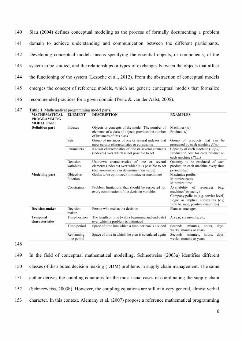
(Pérez et al., 2010; Shapiro, 1993). Table 1 provides a description of mathematical programming 137
model parts. 138
2.2 Conceptual mathematical modelling 139
6
Siau (2004) defines conceptual modeling as the process of formally documenting a problem 140
domain to achieve understanding and communication between the different participants. 141
Developing conceptual models means specifying the essential objects, or components, of the 142
system to be studied, and the relationships or types of exchanges between the objects that affect 143
the functioning of the system (Lezoche et al., 2012). From the abstraction of conceptual models 144
emerges the concept of reference models, which are generic conceptual models that formalize 145
recommended practices for a given domain (Pesic & van der Aalst, 2005). 146
Table 1. Mathematical programming model parts. 147 MATHEMATICAL PROGRAMMING MODEL PART
ELEMENT DESCRIPTION EXAMPLES
Definition part Indexes Objects or concepts of the model. The number of elements of a class of objects provides the number of instances of this class
Machines (m) Products (i)
Sets Group of instances of one or several indexes that meet certain characteristics or constraints
Group of products that can be processed by each machine P(m)
Parameters Known characteristics of one or several elements (indexes) over which is not possible to act
Capacity of each machine (Capm) Production cost for each product on each machine (PCim)
Decision variables
Unknown characteristics of one or several elements (indexes) over which it is possible to act (decision-maker can determine their value)
Quantity to be produced of each product on each machine every time period (Ximt)
Modelling part
Objective function
Goal/s to be optimized (minimize or maximize) Maximize profits Minimize costs Minimize time
Constraints Problem limitations that should be respected for every combination of the decision variables
Availability of resources (e.g. machines’ capacity) Company policies (e.g. service level) Logic or implicit constraints (e.g. flow balance, positive quantities)
Decision-maker Decision-maker
Person who makes the decision Planner, manager
Temporal characteristics
Time-horizon The length of time (with a beginning and end date) over which a problem is optimized
A year, six months, etc.
Time-period Space of time into which a time-horizon is divided Seconds, minutes, hours, days, weeks, months or years
Replanning time period
Space of time in which the plan is calculated again Seconds, minutes, hours, days, weeks, months or years
148
In the field of conceptual mathematical modelling, Schneeweiss (2003a) identifies different 149
classes of distributed decision making (DDM) problems in supply chain management. The same 150
author derives the coupling equations for the most usual cases in coordinating the supply chain 151
(Schneeweiss, 2003b). However, the coupling equations are still of a very general, almost verbal 152
character. In this context, Alemany et al. (2007) propose a reference mathematical programming 153

7
model for collaborative planning that addresses two of the challenges of DDM: the spatial and 154
temporal interdependencies. Alemany et al. (2011) developed an application to support the 155
integrated modelling and execution of the supply chain collaborative planning process made up of 156
several decisional centers which make decisions based on mathematical programming models. 157
However, the formulation of the own specific decisional characteristics of each decision center 158
(micro-decision view) mainly relies on the ability of the mathematical programming modeler. 159
Moreover, Pérez-Perales et al. (2012) propose a framework to support modelling the decisional 160
view of collaborative planning through mathematical programming models. 161
While the above studies are very useful, this article provides further tool-supported guidence and 162
a precise specification in terms of derivation rules to derive mathematical programming models 163
from a conceptual model, as opposed to general descriptions or relying in the modeler’s ability. 164
2.3 Process of mathematical programming model formulation 165
Since conceptual models are not standardized, neither is the process of deriving the mathematical 166
programming model from the concept model, which remains ad hoc. In this sense, Raghunathan 167
(1996) proposed a methodology to design a DSS with its underlying mathematical programming 168
and data models. The methodology includes six steps: (i) problem domain analysis, (ii) database 169
design, (iii) modelbase design, (iv) database/modelbase integration design, (v) problem/decision 170
maker characteristics and (vi) specific DSS design. However, the setting of Raghunathan (1996) 171
is a classroom, so the problem statement is completely specified from the start. Alternatively, our 172
proposal is inspired in the current, agile way of system specification, which recognizes that the 173
construction of any model should be iterative and incremental. Additionally, the use of entity-174
relationship modelling by Raghunathan (1996) has two implications: a) the problem must be 175
simple, otherwise the diagram is not even readable; and b) stakeholders may not be able to 176
understand it. Contrarily, we use a natural language and a semi-structured scenario specification 177

8
for the conceptual model, which is more appealing for a system specification that incorporates 178
stakeholders in the process. 179
Furthermore, Dominguez-Ballesteros et al. (2002) define different stages in the process of 180
deterministic and stochastic linear programming model formulation and implementation: 181
conceptualisation (data collection and study of the problem), data modelling (categorisation and 182
abstraction of the data), algebraic form (modeller’s form), translation (matrix generator/modelling 183
language), machine-readable form (algorithm’s form), solution and solution analysis. However, 184
the stages can be understood as guidelines for the mathematical programming modeler more than 185
a derivation procedure. That is, unlike Raghunathan (1996) and to the best of our knowledge, no 186
methodology or structured modeling language is proposed for the conceptualization stage. 187
2.4 Requirements elicitation 188 189 Requirements elicitation is the process that analysts follow to ensure a correct understanding of 190
stakeholders’ needs and the domain specification before a system is designed and implemented 191
(Leite et al., 2000). In this regard, Geisser and Hildenbrand (2006) state that software requirements 192
are very complex and a multitude of stakeholders participate in their description (Geisser & 193
Hildenbrand, 2006). They propose a method called CoREA that covers collaborative requirements 194
elicitation in a distributed environment as well as quantitative decision support for distributed 195
requirements prioritization and selection. Our proposed approach also relies on collaborative 196
knowledge acquisition and description, with the added advantage of using this knowledge base as 197
a conceptual model from where a mathematical programming model can be derived through the 198
application of a set of rules. 199
Closer to our work, Laporti et al. (2009) propose an approach to develop system requirements in 200
an iterative and collaborative way. Experts in the domain collaborate to build narrative 201
descriptions of stories. Then, these stories are used as input to describe scenarios, which are in 202
turn used to define use cases. In this regard, our proposal is similar since it considers the collective 203

9
construction of LEL + scenarios and a mapping between LEL, scenarios and mathematical 204
programming models. The difference is that the output of the transformation in the work by Laporti 205
et al. (2009) is still a textual, semi-structured representation (use cases), which does not distance 206
much of the previous products, whereas in our case the output is a structured mathematical 207
programming model, so the mapping requires a more complex strategy that includes a precise 208
representation of the relations among model elements. Our approach uses two existing techniques 209
for requirements elicitation: the LEL (Leite & Franco, 1993) and scenarios (Leite et al., 2000). 210
The LEL is a very convenient tool for both stakeholders with no technical skills and analysts, since 211
it conforms to the mechanism used by the human brain to organize knowledge (Oliveira et al., 212
2007), which makes it easy to learn while having good expressiveness. The process to build the 213
LEL is comprised of six steps (Breitman & Leite, 2003; Kaplan et al., 2000), which allow 214
constructing a list of terms classified in four categories (see Table 2). 215
Turning into scenarios, they can be used in different stages of software development, from 216
clarifying business processes and describing requirements to providing the basis of acceptance 217
tests (Alexander & Maiden, 2004). Leite et al. (2000) propose a template with six elements to 218
describe scenarios (see Table 2), which are derived from the LEL following a methodology 219
consisting of five steps: (i) to identify main and secondary actors, i.e., LEL symbols that belong 220
to the subject type; (ii) to identify scenarios within the behavioral responses of symbols chosen as 221
actors; (iii) to define the scenario goal based on the notion of the verb symbol in which the scenario 222
is based; (iv) to identify the scenario resources, searching in the notion of the verb that created the 223
scenario, for LEL symbols of the object category; and (v) to derive episodes from each behavioral 224
response of the verb that identified the scenario. 225
226

10
Table 2. LEL categories and scenarios elements. 227 Category Characteristics Notion Behavioral responses Subject Active elements which perform
actions Characteristics or condition that subject satisfies
Actions that subject performs
Object Passive elements on which subjects perform actions
Characteristics or attributes that object has
Actions that are performed on object
Verb Actions that subjects perform on objects
Goal that verb pursues Steps needed to complete the action
State Situations in which subjects and objects can be located
Situation represented Actions that must be performed to change into another state
Attribute Description Title Name that describes the scenario Goal Conditions and restrictions to be reached after the execution of the scenario Context Conditions and restrictions that are satisfied and constitute the starting point of the scenario
execution. Actors Agents that perform actions during the scenario starting from the context to reach the goal Resources Products and elements used by the actors to perform actions Episodes Steps executed by the actors using the resources starting at the context to reach the goal
228 2.5 Ontologies and knowledge building 229 230 Ontologies define the common vocabulary in which shared knowledge from a domain of discourse 231
is represented (Gruber, 1993; 1995). They can be constructed in two ways, domain dependent and 232
generic. CYC (Lenat, 1995), WordNet (G.A. Miller, 1995) and Sensus (Swartout et al., 1996) are 233
examples of generic ontologies. A benefit of using a domain ontology is to attain the shared and 234
agreed definition of a semantic model of domain data and the links between different types of 235
semantic knowledge, which makes it suitable in formulating data searching strategies for 236
information retrieval (Munir & Sheraz Anjum, 2018). 237
Furthermore, a semantic mediawiki defined over an ontology provides a web-based support for a 238
knowledge building community (Baraniuk et al., 2004). We have used a semantic mediawiki in 239
this work to allow for the collaborative definition of LEL + scenarios of the problem domain and 240
for the semi-automatic derivation of the mathematical programming model using the mediawiki’s 241
query engine. 242

11
3. Methodology for mathematical programming model derivation 243
3.1. Conceptual model construction and methodology overview 244
The mathematical programming model derivation process starts from an existing conceptual 245
model consisting of a complete or close to complete specification of LEL + scenarios of the 246
system. There are three variations that we propose to the original definition of LEL and scenarios 247
for the specific goal of generating mathematical programming models. The first is that we do not 248
use the terms in the “state” category of the LEL, because no mathematical programming model 249
element is derived from them. The second is that we distinguish attributes inside the notion of 250
symbols, especially those that become scenario’s actors and resources. That is, an actor is a LEL 251
subject, and as such it will have a notion with its conceptual definition. We call attributes to the 252
terms that characterize the actors and appear in their notion, usually after the verb “has”. Similarly, 253
a resource is a LEL object with a notion that names its attributes. In turn, attributes are also defined 254
as LEL objects, and this is the reason that attributes are underlined in the notion of the actor or 255
resource that they characterize, describing a relation between LEL terms. The third variation that 256
we propose is related to specifying the temporal location inside scenarios’ context element with 257
more detail, identifying three fields: time horizon, time period and replanning time period. 258
In order to provide a better understanding of the proposed methodology, Figure 1 depicts its two 259
main stages (Conceptual model construction and Mathematical programming model construction), 260
the phases in the construction process for each stage, and two different levels of iteration. There 261
is one iteration cycle that occurs often in the construction of the conceptual model, where scenarios 262
may retrofit the LEL, and a second level or global iteration cycle, between the conceptual model 263
and the mathematical programming model, which should not be as usual. The methodology 264
provides traceability by way of rules that specify the source of each mathematical programming 265
model element. Therefore, this methodology is robust enough to actually afford changes in the 266
mathematical programming model construction. 267

12
The input for the whole process, as Figure 1 shows, is the domain knowledge obtained from 268
stakeholders and documents. The first phase consists in the LEL specification, which is created by 269
a system analyst together with the stakeholders and, if possible, the expert in mathematical 270
modelling, thus creating a multi-disciplinary team. They should identify the sources of knowledge, 271
define the LEL, verify and validate it. The second phase consists in specifying scenarios using the 272
knowledge captured in the LEL. If during the description of the scenario, it is noticed that more 273
knowledge from the domain is needed, the process goes back to phase 1. 274
When the knowledge captured by the LEL + scenarios appears adequate and complete, the third 275
phase (Mathematical Programming Model Derivation) begins. This phase uses the knowledge 276
captured in LEL and scenarios to derive the mathematical model. The mathematical programming 277
derivation proposal consists of several rules that map conceptual model elements (either LEL 278
vocabulary items or scenario elements previously derived from LEL) into mathematical 279
programming model elements. The derivation process may be carried out manually by the 280
mathematical programming expert, possibly together with the system analyst. In addition, we 281
provide tool support for a semi-automatic derivation through a semantic mediawiki. Even with a 282
tool support, manual revision from the mathematical programming expert will be necessary, since 283
it is not possible to automatically create the equations that model constraints from a textual 284
description, although we can isolate the sentence that contains a constraint from the conceptual 285
model. In Fig. 1, the numbering of steps in the mathematical programming model derivation phase 286
denotes a sequence in which rules should be applied. Moreover, at the end of each of these steps, 287
the manual intervention of the mathematical programming expert is advised to prevent an overly 288
complex mathematical programming model (as it could happen with a large number of indexes) 289
or to spot missing items in the conceptual model. Furthermore, it could also be detected that more 290
knowledge from the LEL and Scenarios is needed, and it that case, the process goes back to the 291
conceptual model construction. 292
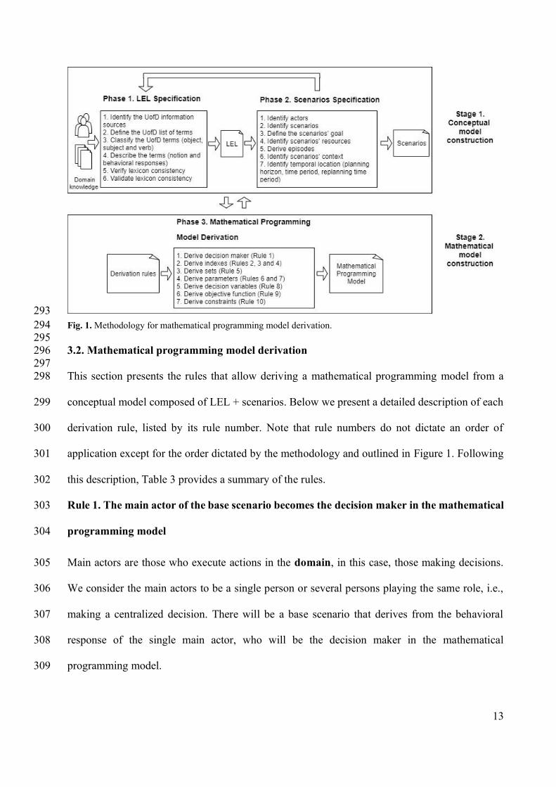
13
293 Fig. 1. Methodology for mathematical programming model derivation. 294 295 3.2. Mathematical programming model derivation 296 297 This section presents the rules that allow deriving a mathematical programming model from a 298
conceptual model composed of LEL + scenarios. Below we present a detailed description of each 299
derivation rule, listed by its rule number. Note that rule numbers do not dictate an order of 300
application except for the order dictated by the methodology and outlined in Figure 1. Following 301
this description, Table 3 provides a summary of the rules. 302
Rule 1. The main actor of the base scenario becomes the decision maker in the mathematical 303
programming model 304
Main actors are those who execute actions in the domain, in this case, those making decisions. 305
We consider the main actors to be a single person or several persons playing the same role, i.e., 306
making a centralized decision. There will be a base scenario that derives from the behavioral 307
response of the single main actor, who will be the decision maker in the mathematical 308
programming model. 309

14
Rule 2. The time period of the planning horizon defined in the temporal location, inside the 310
context of the base scenario, becomes an index of the mathematical programming model. 311
Moreover, other data objects related to time in the temporal location could also become 312
indexes. 313
The base scenario should specify the temporal location in its context attribute. Particularly, the 314
time period specifies the regular intervals in the time horizon at which different decisions are to 315
be made. If such time period exists, Rule 2 is applied to derive an index from it. Other LEL objects 316
specifying time considerations (shipping day or maturity day, among others) could also appear in 317
the temporal location and probably become indexes. 318
Rule 3. Scenarios’ actors that have multiple instances become indexes of the mathematical 319
programming model 320
Actors in scenarios are derived from LEL subjects. A subject in LEL could denote a specific 321
person or a role. If it is a role, which is filled by several persons, there should be an index in the 322
mathematical programming model to represent them. If the cardinality of a particular actor is likely 323
to grow from 1 into several people, the mathematical programming expert could decide to include 324
the index to make the model more flexible to accommodate this change in the near future. 325
Rule 4. Scenarios’ resources that have multiple instances become indexes of the 326
mathematical programming model 327
Resources represent relevant physical elements or information used by scenarios’ actors to achieve 328
their goal. Resources derive from LEL’s objects. Objects can be singletons (a single instance) or 329
denote a class of elements. When an object denotes a class, it becomes an index of the 330
mathematical programming model. Similar to Rule 3, if the object could grow into a class in the 331
future, the mathematical programming expert could decide to include the index. 332

15
Rule 5. Actors and/or resources which are related by a notion in the LEL become sets in the 333
mathematical programming model when their relation denotes a restriction 334
Two or more actors and/or resources are related when they appear in the same notion. In the case 335
where the relation among them is restricted for some cases, this restriction should be defined as a 336
set. Conversely, if the relation is many-to-many, it would not be necessary to define the sets. 337
Rule 6. The number of instances of the indexes could become parameters in the 338
mathematical programming model 339
An actor that becomes an index derives from a LEL subject with multiple instances. The number 340
of instances of an index is known, and therefore, it could become a parameter of the mathematical 341
programming model, although this is not always the case. The same occurs with resources and 342
temporal data objects. An example is the number of instances of the time period, which matches 343
the decision time horizon and could be defined as a parameter. 344
Rule 7. Attributes of scenarios’ actors and attributes of scenarios’ resources and attributes 345
of their relationship with known values become parameters of the mathematical 346
programming model. Each parameter is indexed by those indexes related to it by the same 347
notion and for which its value remains known 348
In the case of attributes that did not become indexes by Rule 4 and denote a known value, by this 349
rule they become parameters of the mathematical programming model. Moreover, a parameter 350
derived by this rule should be indexed by the indexes that are related to it. We define two LEL 351
terms as related if they appear in the same notion, i.e., either one of them appears in the notion of 352
the other, or both terms appear in the notion of a third term. These indexes could include other 353
actors but also other resources. However, note that not all indexes that appear in the notion will be 354
assigned to the parameter, only those that refer to a known value. Thus, the mathematical 355
programming expert should determine which subset of indexes refers to a known value, and the 356

16
parameter should be indexed only by that subset of indexes. The notion gives the whole subset, 357
but the expert decides what indexes should be used. 358
Rule 8. Attributes of scenarios’ actors and attributes of scenarios’ resources and attributes 359
of their relationship that have unknown values become decision variables of the 360
mathematical programming model. Each decision variable is indexed by those indexes 361
related to it by the same notion and for which its value is unknown 362
This rule is similar to Rule 7 but for unknown values. That is, attributes that appear in the notion 363
of actors or resources, which values should be assigned in the decision process, become decision 364
variables. Moreover, decision variables should take the indexes that are related to it by the same 365
notion and refer to unknown values. It could be necessary to define artificial decision variables 366
(without economic/physical interpretation) in order to mathematically represent a reality or to 367
force some logical constraint. 368
Rule 9. The goal of the base scenario contains the objective function 369
The base scenario should specify in its goal attribute, the purpose of the main actor (which 370
becomes the decision maker by Rule 1) in executing the scenario. This goal is specified as a 371
complex sentence with a relative clause that starts with “so as to” followed by the verb “minimize” 372
or “maximize”. From this verb to the end, this relative clause becomes the objective function. 373
Moreover, the expert may look for further details of each objective function in the notion of the 374
LEL symbols involved in the goal. 375
Rule 10. The set of context sentences of all scenarios become the set of constraints of the 376
mathematical programming model 377
Scenarios should specify in its context attribute, the conditions to comply. These conditions are 378
described in natural language, as sentences that relate to the actors and resources of each scenario. 379
17
Experts in mathematical programming modeling should use the restrictions described in the 380
scenarios’ context and relate them to parameters and indexes previously defined by other rules to 381
derive the set of mathematical programming model constraints. These constraints usually contain 382
logical constraints that represent business rules. These rules should appear during the requirements 383
elicitation that a system analyst carries out to construct the LEL, and therefore they would also be 384
derived as part of the scenarios’ context. Additionally, there are added other artificial constraints 385
(for instance, a positive boundary to variables) in order to avoid erroneous results. These 386
constraints will not generally appear in the conceptual model and they should be added by a 387
subsequent analysis of the mathematical programming expert. 388
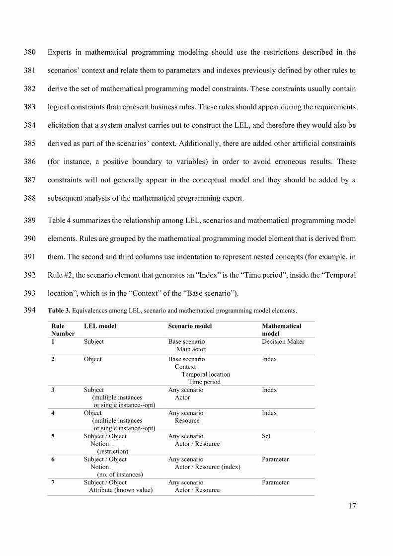
Table 4 summarizes the relationship among LEL, scenarios and mathematical programming model 389
elements. Rules are grouped by the mathematical programming model element that is derived from 390
them. The second and third columns use indentation to represent nested concepts (for example, in 391
Rule #2, the scenario element that generates an “Index” is the “Time period”, inside the “Temporal 392
location”, which is in the “Context” of the “Base scenario”). 393
Table 3. Equivalences among LEL, scenario and mathematical programming model elements. 394
Rule Number
LEL model Scenario model Mathematical model
1 Subject Base scenario Main actor
Decision Maker
2 Object Base scenario Context Temporal location Time period
Index
3 Subject (multiple instances or single instance--opt)
Any scenario Actor
Index
4 Object (multiple instances or single instance--opt)
Any scenario Resource
Index
5 Subject / Object Notion (restriction)
Any scenario Actor / Resource
Set
6 Subject / Object Notion (no. of instances)
Any scenario Actor / Resource (index)
Parameter
7 Subject / Object Attribute (known value)
Any scenario Actor / Resource
Parameter

18
Attribute
8 Subject / Object Attribute (unknown value)
Any scenario Actor / Resource Attribute
Decision Variable
9 Subject Behavioral response (verb)
Base scenario Goal
Objective function
10 Object Any context Constraint
4. Application 395
This section applies the above methodology to the problem of fresh tomato packing addressed by 396
Miller et al. (1997). The purpose of using an existing problem is to contrast the result of our 397
derivation rules with a real, published mathematical programming model while avoiding the long 398
description that a new mathematical program would require. 399
4.1 Conceptual model of the tomato packing problem: LEL + scenarios 400
This section presents the conceptual model for the tomato packing problem created in terms of 401
LEL + scenarios. The team assembled for this task was multidisciplinary, that is, composed of 402
system analysts and a mathematical programming expert. The information sources of the UofD to 403
construct the LEL were provided by the article from Miller et al. (1997), interviews with local 404
tomato producers that played the role of customers and other documentation sources online. After 405
three iterations, the team arrived at the LEL that appears in Table 4. 406
Table 4. LEL of the tomato packing problem. 407 Term Role Notion Packinghouse management (PM)
Subject Conducts the business of the packinghouse. The PM decides when to harvest tomatoes matured in the present or previous cycle, communicates its decision to growers and packs the harvested tomatoes to fulfil the market demand
Grower Subject Person responsible for a tomato field (has been assigned a certain number of acres of tomatoes), including harvesting the tomatoes, for which it has some harvest capacity. There are several growers. Each grower produces a certain yield of bins of tomatoes per acre to take them to the packinghouse
Market Subject Customers of the packinghouse, who buy tomatoes to sell them. The market has a market demand in number of boxes of tomatoes they would like to buy each day
Acres of tomatoes Object Land assigned to a grower with tomatoes that get matured on a certain maturity day, and are harvested on a certain harvesting day. Acres may have a fraction of “vine ripe
tomatoes” that are sold “as is” Tomato Object Produce planted by growers on the acres of their fields. Tomatoes that have not been
harvested in 2 cycles generate a cost of damaged tomato Harvesting day Object Day in which tomatoes already matured are harvested. Every day in the horizon may be
a harvesting day Maturity day Object Day in a period in which tomatoes in an acre get ready to be harvested. The acres of a
specific grower may have different maturity days within the decision horizon

19
Decision horizon Object Largest time in which the readiness of tomato fields for harvest can be accurately predicted. It is 3 days
Harvest capacity Object The capacity of a grower to harvest during a certain day Bin Object Container where the grower places the harvested tomatoes Cost of damaged tomato Object Penalty cost due to dissatisfaction of a grower because of delayed harvest of fields
matured in the previous and present cycles in $ per bin Fraction of “vine ripe
tomatoes” (v.r.t.) Object Tomatoes sold without gassing
Yield of bins of tomatoes per acre
Object The number of bins of harvested tomatoes per acre of a certain grower
Packinghouse Object Place where tomatoes are packed in boxes and stored. It has a packing capacity, and a gassing capacity per day. The packinghouse requires some fraction of hour needed to pack a bin at a certain packing cost. The packinghouse generates a fraction of tomatoes ready after gassing. The packinghouse works on regular hours (9 to 5) and overtime hours (after 5pm) to generate an inventory level at the end of the day
Packing cost Object The total packing cost consist of: (1) cost of damaged tomatoes; (2) inventory holding cost, (3) shortfall cost, (4) overtime and (5) regular hour packing costs
Packing capacity Object No more tomatoes may be packed once the packinghouse reaches the packing capacity Gassing capacity Object Capacity of the packinghouse to gass tomatoes in a harvesting day. It is measured in
number of boxes of tomatoes Fraction of hour needed to pack a bin
Object Time required for packing 1 bin of harvested tomatoes and put them in boxes
Fraction of tomatoes ready after gassing
Object Tomatoes ready after a gassing session
Regular packing hours Object Hours when the packinghouse is operating on a day, that generates a regular packing cost. It goes from 9 am to 5 pm
Overtime packing hours Object Extra hours required to complete the packing at the packinghouse on a day. They generate a higher cost than the regular packing hours. Overtime hours are after 5pm
Regular packing cost Object Cost of packinghouse operation in $ per hour during regular packing hours Overtime packing cost Object Cost of packinghouse operation in $ per hour during overtime packing hours Inventory level Object Number of boxes of tomatoes of the packinghouse at the end of a certain day. It has a
certain inventory holding cost in box/day Inventory holding cost Object Cost of packinghouse storage in boxes/day Market demand Object Number of boxes of tomatoes that the packinghouse customers require in each harvesting
day. If the market demand is not covered it generates a shortfall Shortfall Object Number of missing boxes of tomatoes needed to reach the market demand on a certain
harvesting day Shortfall cost Object Cost of being short on satisfying the market demand in $ per box short Box Object Container where tomatoes are placed during packing Harvest Verb To cut the tomatoes that are matured Pack Verb Put in boxes the harvested tomatoes. Packing is done on regular hours at a certain cost
or overtime hours to complete packing all harvested tomatoes Gass Verb Technique used to ripen tomatoes that are not completely matured by exposing them to
ethylene gas
408 The first version of the scenarios was created after the first iteration of the LEL and was used to 409
retrofit the second iteration of the LEL. 410
The following four tables describe the scenarios of the tomato packing problem. First, Table 5 411
presents the sole Level 0 scenario, called base scenario. Then, Tables 6 through 8 show the three 412
scenarios of Level 1, which derive from episodes of the base scenario. 413
414

20
Table 5. Scenario Level 0 of the tomato packing problem. 415 Scenario 0: Plan the harvest and the packing of fresh tomatoes Goal Make a plan at the beginning of the present cycle to harvest and pack tomatoes matured on the present and last
cycles, so as to minimize the total packing cost Actors Main actor Packinghouse management (PM) Secondary actors Growers, market Resources Physical resources Packinghouse; acres of matured tomatoes for each grower in the present and past cycles;
tomatoes; bins; boxes. Information
resources Market demand in number of boxes for each day in the present cycle; for each grower, the number of acres of matured tomatoes in the present and past cycles and the number of bins of tomatoes generated after harvesting.
Context - Not all tomatoes that get matured in a cycle are harvested in the same cycle. - Tomatoes harvested in the next cycle after they get matured may be sold but have less quality. - Tomatoes not harvested in the next cycle after they get matured must be discarded. - A grower may only harvest up to their capacity. - The packinghouse may only pack and gass a limited number of tomato boxes a day. - Temporal location: • Decision horizon: 3 days • Decision period: harvesting day; every day in a decision horizon. • Other temporal variables: maturity day; any day in the decision horizon.
Episodes - PM makes a plan with the harvesting day of matured tomatoes, for each day in the present cycle, in number of acres for each grower. - Each grower harvests the amount decided and communicated by the PM. - Each grower takes the harvested tomatoes in bins to the packinghouse. - PM packs the harvested tomatoes in the packinghouse, labelling some boxes as “vine-ripe tomatoes”. - PM gasses all boxes of tomatoes which are not labelled as “vine ripe”. - Tomato boxes are shipped to cover the market demand, and the surplus remains as inventory of the packinghouse.
Table 6. Scenario 1.1 at Level 1 of the tomato packing problem. 416 Scenario 1.1: Plan the the harvesting day of matured tomatoes
Goal Decide how many acres of matured tomatoes to harvest for each grower in each day of the present cycle Actors Main actor Packinghouse management (PM) Resources Physical resources Acres of tomatoes. Information
resources For each grower: harvest capacity, acres of matured tomatoes for each day and yields of bins of tomatoes per acre. Also: cost of tomatoes damaged due to delayed harvest, packing and gassing capacity of the packing house.
Context - A grower may only harvest in a day up to their harvest capacity. - The number of bins of harvested tomatoes to pack from all growers should be less than the available gassing capacity of the packinghouse for that day. - The number of bins of harvested tomatoes to be packed per day should be less than the combined regular and overtime packing capacity of the packinghouse.
Episodes - Considering the information resources available, the PM calculates, for each day in the present cycle and for each grower, the number of acres to harvest of tomatoes matured of the previous and the present cycles.
Table 7. Scenario 1.2 at Level 1 of the tomato packing problem. 417 Scenario 1.2: Harvest Goal Harvest the tomatoes and take them to the packinghouse. Actors Main actor Grower Resources Physical resources Acres of tomatoes; tomatoes; bins; packinghouse. Information
resources Harvest capacity; acres of matured tomatoes for each day; number of acres to harvest each day
Context - Tomatoes to be harvested are matured. Episodes - The grower cuts the tomatoes from the acres already matured that the PM decided to cut on the present day.
- The grower places the tomatoes in bins. - The grower takes the bins to the packinghouse.
418

21
Table 8. Scenario 1.3 at Level 1 of the tomato packing problem. 419 Scenario 1.3: Pack the harvested tomatoes Goal Put the tomatoes in boxes to be transported. Actors Main actors Packinghouse personnel Resources Physical resources Bins of tomatoes; boxes; packinghouse. Information
resources Gassing capacity; regular packing hours; regular packing hour cost; overtime packing hours; overtime packing hour cost
Context - Packing occurs during regular packing hour plus overtime packing hours, which combined are at most 12 hours. - Regular packing hours are at most 8 hours a day, and overtime packing hours are at most 4 hours a day. - No more tomatoes may be packed once the packinghouse reaches the packing capacity
420
4.2 Derived mathematical programming model 421
We show the derived mathematical programming model elements in separate tables according to 422
the rules applied. First, Table 9 shows the decision maker and indexes generated by applying Rules 423
1 – 4. 424
Table 9. Derivation of decision maker and indexes. 425 Rule Number
LEL model Scenario model Mathematical programming model
1 Subject: Packinghouse Management (PM)
Scenario 0 Main actor PM
Decision Maker PM
2 Object: Harvesting day Scenario 0 Context Temporal location Decision period
Indexes t
2 Object: Maturity day Scenario 0 Context Temporal location Other temporal vars
j
3 Subject: Grower Scenario 0 and 1.2 Actor: Grower
i
426 In the process of deriving the indexes, some scenarios’ resources with multiple instances were 427
considered as candidates on which to apply Rule 4. After that, the expert reviewed the relations 428
among actors and resources but did not derive any sets because there are none restricted relations. 429
Applying Rule 6 to the number of instances of the index for time period t yielded the time horizon 430
as the parameter T. The number of instances of the index for maturity day j is the same parameter 431
T. The number of instances of the index for grower i yielded parameter K. Other parameters came 432
from analyzing the attributes of scenarios’ actors and resources. For example, the attribute acres 433
of actor grower yielded parameter H. Rule 7 indicates that H should be indexed by the indexes 434

22
“related to it by the same notion”. In this case, the expert inspected the notion of acres looking the 435
underlined terms (i.e., related elements) that were defined as indexes: i for “grower”, j for 436
“maturity day” and t for “harvesting time”. However, the known values of acres are their grower 437
and their maturity day, but their harvesting time is unknown. Therefore, the indexes assigned to 438
the parameter are i and j, and the parameter is Hij. Other parameters were derived similarly. The 439
whole list of parameters appears in Table 10. 440
Table 10. Derivation of parameters. 441 Rule Number
LEL model Scenario model Mathematical programming model parameter
6 Object: Harvesting day Index: t
Scenario 0 Context Temporal location Decision period
T
6 Subject: Grower Index: i
Scenario 0 and 1.2 Actor: Grower
K
7 Subject: Grower Attribute: Acres Related indexes: Grower (i), Maturity day (j)
Scenario 0 and 1.2 Actor: Grower Attribute: Acres
Hij
7 Subject: Grower Attr: Harvest capacity Related indexes: i
Scenario 0 and 1.2 Actor: Grower Attr: Harvest capacity
Ui
7 Subject: Grower Attr: Yields of bins Related indexes: i
Scenario 0 and 1.2 Actor: Grower Attr: Yields of bins
bi
7 Subject: Market Attr: Market demand Related indexes: Harvesting day (t)
Scenario 0 Actor: Market Attr: Market demand
Dt
7 Object: Acres Attr: Fraction of v.r.t. Related indexes: -
Scenario 0 Resource: Acres Attr: Fraction of v.r.t.
7 Object: Packinghouse Attr: Packing capacity Related indexes: -
Scenario 0 Resource: Packinghouse Attr: Packing capacity
P
7 Object: Packinghouse Attr: Gassing capacity Related indexes: t
Scenario 0 Resource: Packinghouse Attr: Gassing capacity
Gt
7 Object: Packinghouse Attr: Packing cost Notion: Cost of damaged tomato Related indexes: -
Scenario 1.3 Resource: Packinghouse Attr: Packing cost Notion: Cost of damaged tomato
C
7 Object: Packinghouse Attr: Packing cost Notion: Inventory holding cost Related indexes: -
Scenario 1.3 Resource: Packinghouse Attr: Packing cost Notion: Inventory holding cost
Ch

23
7 Object: Packinghouse Attr: Packing cost Notion: Shortfall cost Related indexes: -
Scenario 1.3 Resource: Packinghouse Attr: Packing cost Notion: Shortfall cost
Cs
7 Object: Packinghouse Attr: Packing cost Notion: Regular packing cost Related indexes: -
Scenario 1.3 Resource: Packinghouse Attr: Packing cost Notion: Regular packing cost
Cr
7 Object: Packinghouse Attr: Packing cost Notion: Overtime packing cost Related indexes: -
Scenario 1.3 Resource: Packinghouse Attr: Packing cost Notion: Overtime packing cost
Co
7 Object: Packinghouse Attr: Fraction of hour needed to pack a bin Related indexes: -
Scenario 0 Resource: Packinghouse Attr: Fraction of hour needed to pack a bin
f
7 Object: Packinghouse Attr: Fraction of tom. ready after gassing Related indexes: -
Scenario 0 Resource: Packinghouse Attr: Fraction of tom. ready after gassing
α
442 The next step was to derive the decision variables from the analysis of the attributes of scenarios’ 443
actors and resources, but this time, with unknown values. For example, the attribute acres of actor 444
grower, with a certain maturity day and with an uncertain harvesting day. This attribute yielded 445
decision variable X. Similar to the case for parameter H, to find the indexes for variable X the 446
expert looked at the underlined indexes in notion of acres, which are: i for grower, j for maturity 447
day and t for harvesting time, and the 3 of them are assigned to X to yield Xijt. Other decision 448
variables were derived similarly by applying Rule 8 (It, Rt, Ot, St), and appear in Table 11. Further 449
analysis on the scenarios and the context, caused the expert to split the decision variable Xijt in 2 450
variables: Xijt to refer to the acres matured on the present cycle and Lijt to refer to the acres matured 451
on the last cycle. Additionally, 2 more decision variables were needed to represent the acres not 452
harvested, both in the present cycle (Yijt) and the past cycle (Aijt). 453
To define the objective function1, Rule 9 was applied. Then, the expert had to manually write the 454
final equation: 455
Minimize 456
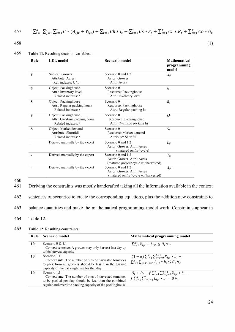
24
∑ ∑ ∑ 𝐶 ∗ (𝐴𝑖𝑗𝑡𝑇𝑡=1
𝑇𝑗=1 + 𝑌𝑖𝑗𝑡)𝐾
𝑖=1 + ∑ 𝐶ℎ ∗ 𝐼𝑡𝑇𝑡=1 + ∑ 𝐶𝑠 ∗ 𝑆𝑡 + ∑ 𝐶𝑟 ∗ 𝑅𝑡 + ∑ 𝐶𝑜 ∗ 𝑂𝑡
𝑇𝑡=1
𝑇𝑡=1
𝑇𝑡=1 457
(1) 458
Table 11. Resulting decision variables. 459 Rule LEL model Scenario model Mathematical
programming model
8 Subject: Grower Attribute: Acres Rel. indexes: i, j, t
Scenario 0 and 1.2 Actor: Grower Attr.: Acres
Xijt
8 Object: Packinghouse Attr.: Inventory level Related indexes: t
Scenario 0 Resource: Packinghouse Attr.: Inventory level
It
8 Object: Packinghouse Attr.: Regular packing hours Related indexes: t
Scenario 0 Resource: Packinghouse Attr.: Regular packing hs
Rt
8 Object: Packinghouse Attr.: Overtime packing hours Related indexes: t
Scenario 0 Resource: Packinghouse Attr.: Overtime packing hs
Ot
8 Object: Market demand Attribute: Shortfall Related indexes: t
Scenario 0 Resource: Market demand Attribute: Shortfall
St
- Derived manually by the expert
Scenario 0 and 1.2 Actor: Grower. Attr.: Acres (matured on last cycle)
Lijt
- Derived manually by the expert Scenario 0 and 1.2 Actor: Grower. Attr.: Acres (matured present cycle not harvested)
Yijt
- Derived manually by the expert Scenario 0 and 1.2 Actor: Grower. Attr.: Acres (matured on last cycle not harvested)
Aijt
460 Deriving the constraints was mostly handcrafted taking all the information available in the context 461
sentences of scenarios to create the corresponding equations, plus the addition new constraints to 462
balance quantities and make the mathematical programming model work. Constraints appear in 463
Table 12. 464
Table 12. Resulting constraints. 465 Rule Scenario model Mathematical programming model
10 Scenario 0 & 1.1 Context sentence: A grower may only harvest in a day up to his harvest capacity.
∑ 𝑋𝑖𝑗𝑡𝐾𝑖=1 + 𝐿𝑖𝑗𝑡 ≤ 𝑈𝑖 ∀𝑖𝑡
10 Scenario 1.1 Context sntc: The number of bins of harvested tomatoes to pack from all growers should be less than the gassing capacity of the packinghouse for that day.
(1 − 𝛿) ∑ ∑ 𝑋𝑖𝑗𝑡𝑇−1𝑡−𝑗=0
𝐾𝑖=1 ∗ 𝑏𝑖 +
∑ ∑ 𝐿𝑖𝑗𝑡𝑇𝑡+𝑇−𝑗=1
𝐾𝑖=1 ∗ 𝑏𝑖 ≤ 𝐺𝑡 ∀𝑡
10 Scenario 1.1 Context sntc: The number of bins of harvested tomatoes to be packed per day should be less than the combined regular and overtime packing capacity of the packinghouse.
𝑂𝑡 + 𝑅𝑡 − 𝑓 ∑ ∑ 𝑋𝑖𝑗𝑡𝑇−1𝑡−𝑗=0
𝐾𝑖=1 ∗ 𝑏𝑖 −
𝑓 ∑ ∑ 𝐿𝑖𝑗𝑡𝑇𝑇−𝑗=1
𝐾𝑖=1 ∗ 𝑏𝑖 = 0 ∀𝑡

25
10 Scenario 1.3 Context sntc: Packing occurs during regular packing hour plus overtime packing hours, which are at most 12 hours.
𝑂𝑡 + 𝑅𝑡 ≤ 12 ∀𝑡
10 Scenario 1.3 Context sntc: Regular packing hs. are at most 8 hours/day
𝑅𝑡 ≤ 8 ∀𝑡
- Added by expert: balance the acres matured in the previous cycle but not yet harvested
𝐴𝑖𝑗𝑡 − 𝐴𝑖𝑗𝑡−1 + 𝐿𝑖𝑗𝑡 = 0 ∀𝑖𝑗𝑡
- Added by expert: balance the acres matured in the present cycle but not yet harvested
𝑌𝑖𝑗𝑡 − 𝑌𝑖𝑗𝑡−1 + 𝑋𝑖𝑗𝑡 = 𝐻𝑖𝑗 ∀𝑖𝑗𝑡
- Added by expert: balance the end-of-period inventory level (equal to the preceding end-of-period level + the quantity of “vine ripe” tomatoes packed + the number of boxes of
tomatoes ready after gassing - the forecasted demand)
𝐼𝑡 − 𝑆𝑡 − 𝐼𝑡−1 + 𝑆𝑡−1 − 𝛿 ∑ ∑ 𝑋𝑖𝑗𝑡𝑇−1𝑡−𝑗=0
𝐾𝑖=1 ∗ 𝑏𝑖 +
𝛿 ∑ ∑ 𝐿𝑖𝑗𝑡𝑇𝑡−𝑇−𝑗=1
𝐾𝑖=1 ∗ 𝑏𝑖 = 𝐷𝑡 + 𝐺𝑡 ∀𝑡
- Added by expert: assure a continual flow of tomatoes to the market. The mature green tomatoes to be packed should be at least equal to a fraction α of tomatoes ready on the day
of gassing.
(1 − 𝛿) ∑ ∑ 𝑋𝑖𝑗𝑡𝑇−1𝑡−𝑗=0
𝐾𝑖=1 ∗ 𝑏𝑖 +
∑ ∑ 𝐿𝑖𝑗𝑡𝑇𝑡+𝑇−𝑗=1
𝐾𝑖=1 ∗ 𝑏𝑖 ≥ 𝛼𝐺𝑡 ∀𝑡
5. Semantic mediawiki construction for the LEL and scenarios definition 466
A domain ontology is proposed to attain the shared and agreed definition of a semantic model for 467
the LEL and scenarios. Moreover, ontology-based information retrieval allows us to formulate 468
queries based on our derivation rules, which will help in the semi-automatic derivation of 469
mathematical programming model elements. Finally, tool support is provided through a semantic 470
mediawiki constructed over the ontology, which allows for the knowledge building process of a 471
conceptual model and its derivation into math model elements. 472
5.1 Ontology Model 473
The proposed ontology is depicted in Figure 2. Thus, Subjects symbols are related to Scenario’s 474
Actors while Objects symbols are related to Scenario’s Resources. Moreover, Verbs symbols are 475
related to Scenario and Episode from Scenario’s representation as they represent the activities or 476
actions that are realized. LEL symbols are represented by the Symbol element, that has two 477
properties: a notion and a list of behavioral responses. Thus, the notion property just contains has 478
relations with Subjects and Objects that represent attributes of the described Symbol. Since we 479
need to differentiate known attributes (parameters) from unknown ones (decision variables), the 480
has relation is in fact modeled as two separate relations: has known and has unknown. In turn, the 481

26
behavioral response of a LEL’s Symbol is represented using a relation to the Verbs that represent 482
the actions were the Symbol participates, and therefore, its responsibilities. 483
From the scenario’s perspective, the element Scenario is represented by a property to define a title 484
as plane text. The rest of the Scenario’s properties are represented as relations with other model 485
elements. Thus, there is a relation called bounded to a Context. There are two relations from 486
Scenario to the Actor element called involves main actor and involves secondary actor, to 487
represent the main and secondary actors of the Scenario respectively. Scenario also has a property 488
called executed over, to related it with the Resources over which it is executed. The Scenario’s 489
episodes are described by the property performs related with the Episode elements. Finally, 490
Scenarios are connected by the property has to the Goal element. 491
In turn, a Context has a text property description and a has property related to a TemporalLoc that 492
represents the temporal location of the scenarios with its properties for time-horizon, time_period 493
and replanning_time_period. The Actor element has name and instance_number as properties, 494
where the latter is used for the mathematical programming model derivation, to identify actors 495
with more than one instance as indexes. Resource has a structure identical to Actor although their 496
semantic meaning is completely different. The Episode element has a sentence that describes it 497
and a relation described in that connects the Episodes to the parent Scenario. Moreover, a Goal 498
has a property description and a relation optimize to an Optimization Goal. This Optimization 499
Goal is not part of the original definition of scenarios but added for mathematical programming 500
model derivation purposes. It is described by two properties: Operation and TargetVariable to 501
define the max/min operation for one particular variable as objective of the Scenario’s Goal. 502
Finally, there is a Constraint element that could be related with Episode, Actor, Resource or 503
TemporalLoc elements by the property is restricted by. A Constraint is defined by the property 504
expression, which is applied on the corresponding elements. 505

27
506 Fig. 2. The LEL and scenarios ontology. 507 508 5.2 Semantic queries 509
The queries rely on the definition of a specific Scenario instance defined as Base Scenario. The 510
result of these queries will be used by the mathematical programming expert to obtain a 511
preliminary version of the final mathematical programming model, as explained before. Table 13 512
summarizes the queries, in a pseudo-code that makes them more readable. 513
Table 13. Queries based on each rule to derive potential mathematical programming model elements 514 Rule Number
Mathematical model output
Semantic Query
1 Decision Maker Base Scenario involves main actor: ?Actor
2 Index
Base Scenario bounded: ?Context ?Context has: ?TemporalLoc ?time_period
3 Index Scenario involves main actor: ?Actor ?Actor instance_number >1: ?Actor Scenario involves secondary actor: ?Actor ?Actor instance_number >1: ?Actor
4 Index Scenario executed over: ?Resource ?Resource instance_number > 1: ?Resource
5 Set Symbol has known: ?Attribute1 Symbol has known: ?Attribute2 (?Attribute1 is restricted by: ?Constraint) == (?Attribute2 is restricted by: ?Constraint) ?Attribute1, ?Attribute2
6 Parameter Scenario executed over: ?Resource ?Resource instance_number > 1: ?Resource instance_number Scenario involves secondary actor: ?Actor ?Actor instance_number > 1: ?Actor instance_number
28
7 Parameter (Actor has known: ?Attribute)+ (Resource has known: ?Attribute)
8 Decision Variable (Actor has unknown: ?Attribute)+ (Resource has unknown: ?Attribute)
9 Objective function Base Scenario has: ?Goal ?Goal optimize: ?Optimization Goal
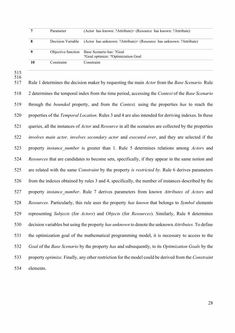
10 Constraint Constraint
515 516 Rule 1 determines the decision maker by requesting the main Actor from the Base Scenario. Rule 517
2 determines the temporal index from the time period, accessing the Context of the Base Scenario 518
through the bounded property, and from the Context, using the properties has to reach the 519
properties of the Temporal Location. Rules 3 and 4 are also intended for deriving indexes. In these 520
queries, all the instances of Actor and Resource in all the scenarios are collected by the properties 521
involves main actor, involves secondary actor and executed over, and they are selected if the 522
property instance_number is greater than 1. Rule 5 determines relations among Actors and 523
Resources that are candidates to become sets, specifically, if they appear in the same notion and 524
are related with the same Constraint by the property is restricted by. Rule 6 derives parameters 525
from the indexes obtained by rules 3 and 4, specifically, the number of instances described by the 526
property instance_number. Rule 7 derives parameters from known Attributes of Actors and 527
Resources. Particularly, this rule uses the property has known that belongs to Symbol elements 528
representing Subjects (for Actors) and Objects (for Resources). Similarly, Rule 8 determines 529
decision variables but using the property has unknown to denote the unknown Attributes. To define 530
the optimization goal of the mathematical programming model, it is necessary to access to the 531
Goal of the Base Scenario by the property has and subsequently, to its Optimization Goals by the 532
property optimize. Finally, any other restriction for the model could be derived from the Constraint 533
elements. 534

29
5.3 Mediawiki implementation 535
We have built a semantic mediawiki in order to provide support for the collaborative construction 536
of a knowledge base. The wiki provides the capability of creating and editing articles by way of a 537
user-friendly interface guided by forms that will be used by stakeholders, analysts and 538
mathematical modelling experts. These forms are based on the ontology proposed for the LEL and 539
scenarios. Figure 3 shows a form to describe a Scenario. The figure shows that some attributes as 540
goal and context are plain text, while others are described with a kind of button or token. These 541
tokens describe relations to other elements of the model already created. 542
543 Fig. 3. Mediawiki form based on LEL and scenarios’ ontology. 544 545 In turn, Figure 4 shows a form to navigate a Scenario. The wiki-links could be blue or red 546
describing whether the related article is already defined or not, respectively. 547

30
548 Fig. 4. Scenario’s article. 549 550 Finally, the capability of application of ontologies as a semantic knowledge model allows to 551
implement the semantic queries described previously to semi-automatically derive mathematical 552
programming model elements from LEL + scenarios elements. Thus, once the knowledge base is 553
constructed, the mathematical modelling expert will be able to generate new articles with a 554
preliminary version of the mathematical programming model. Figures 5 displays an example, with 555
the article generated from the LEL and scenarios of the case study. Note that the support is not 556
completely automatic because the inference only allows for an approximation to the mathematical 557
programming model, and the expert is still needed to verify the correctness of the mediawiki 558
derivation and provide the algebraic form. 559

31
560
561 Fig. 5. Article of mediawiki with automatic mathematical programming model derivation. 562 563 6. Conclusions 564
This paper has presented a novel methodology that connects the areas of requirements engineering 565
with conceptual modelling in order to build mathematical programming models that capture the 566
business domain more effectively and completely. Specifically, the methodology has proposed for 567
the first time the use of the LEL and scenarios for creating a conceptual model of a domain from 568
32
where a mathematical programming model can be derived. The construcion of the conceptual 569
model invites the participation of all stakeholders, which is deficiency of other proposals for DSS 570
construction in agriculture. In comparison with other approaches for conceptual mathematical 571
modelling, this article provides further tool-supported guidence about how to obtain the problem 572
definition and how to derive a mathematical programming model from a precise specification in 573
terms of derivation rules, as opposed to relying on mere textual descriptions or in the modeler’s 574
ability. Moreover, we have proposed an ontology that provides the basis for a semantic mediawiki 575
that serves both, sharing knowledge of the conceptual domain model among the different 576
stakeholders, as well as semi-automating the derivation of the mathematical programming model. 577
The usefulness of this proposal can be understood from several perspectives: research, academic 578
and managerial. From the research and academic points of view, we may highlight the main 579
contributions as follows: (i) it provides a novel step-by-step methodology based on the LEL and 580
scenarios that allows both: to obtain the required information to derive the definition part of a 581
mathematical programming model, and to define the optimization problems that constitute the 582
modelling part of the model; (ii) our approach provides a structure to the problem that allows to 583
identify the elements of the problem clearly; (iii) using the LEL and scenarios to create a 584
conceptual model iteratively and incrementally in collaboration with stakeholders allows applying 585
an agile development approach to mathematical modelling; (iv) the use of LEL and scenarios 586
provides traceability from the requirements to the mathematical programming model 587
implementation to cope with possible changes of requirements and a better understanding of their 588
impact on the model; and (v) the process of creating a conceptual model with LEL + scenarios 589
also generates a complete specification of requirements for a potential model-based DSS. 590
Regarding the managerial perspective, we believe that the ease of use and good expressiveness of 591
the proposed methodology will facilitate the implementation of mathematical programming 592
models in agriculture, as well as provide new tools for teaching mathematical programming and 593
33
foster research in the combined areas of agile methods in requirements engineering, mathematical 594
programming and decision support system development. Further research includes validating the 595
proposed methodology in real world case studies from agriculture. Finally, we intend to extend 596
the approach to the derivation of mathematical programming models under uncertainty, such as 597
stochastic programming and fuzzy mathematical programming. 598
Acknowledgments. This work was supported by the European Commission, project H2020- 599 RUC-APS, grant number H2020-MSCA-RISE-2015-691249; and the Argentinian National 600 Agency for Scientific and Technical Promotion (ANPCyT), grant number PICT-2015-3000. 601
References 602 Alemany, M., Ortiz, A. & Fuertes-Miquel, V.S. (2018). A decision support tool for the order 603
promising process with product homogeneity requirements in hybrid Make-To-Stock and 604 Make-To-Order environments. Application to a ceramic tile company. Computers & 605 Industrial Engineering 122: 219–234. 606
Alemany, M.M.E., Alarcón, F., Lario, F.C. & Boj, J.J. (2011). An application to support the 607 temporal and spatial distributed decision-making process in supply chain collaborative 608 planning. Computers in Industry 62: 519–540. 609
Alemany, M.M.E., Lario, F.C., Ortiz, A. & Gómez, F. (2013). Available-To-Promise modeling 610 for multi-plant manufacturing characterized by lack of homogeneity in the product: An 611 illustration of a ceramic case. Applied Mathematical Modelling 37(5): 3380–3398. 612
Alemany, M.M.E., Pérez Perales, D., Alarcón, F. & Boza, A. (2007). Planificación Colaborativa 613 para Redes de Suministro-Distribución (RdS/D) mediante programación matemática en 614 entornos distribuidos. In Int. Conference on Industrial Engineering & Industrial 615 Management. 616
Alexander, I. & Maiden, N. (2004). Scenarios, stories, and use cases: the modern basis for system 617 development. Computing Control Engineering Journal 15(5): 24–29. 618
Armengol, A., Mula, J., Díaz-Madroñero, M. & Pelkonen, J. (2015). Conceptual model for 619 associated costs of the internationalisation of operations. Lecture Notes in Management and 620 Industrial Engineering 181–188. 621
Baraniuk, R., Burrus, C., Johnson, D. & Jones, D. (2004). Sharing knowledge and building 622 communities in signal processing. IEEE Signal Processing Magazine 21(5): 10–16. 623
Behzadi, G., O’Sullivan, M.J., Olsen, T.L. & Zhang, A. (2018, September 1). Agribusiness supply 624 chain risk management: A review of quantitative decision models. Omega (United Kingdom). 625 Elsevier Ltd. 626
Breitman, K.K. & Leite, J.C.S.P. (2003). Ontology as a requirements engineering product. In 627 Proceedings of the IEEE Int. Conference on Requirements Engineering (RE). 628
Cid-Garcia, N.M. & Ibarra-Rojas, O.J. (2019). An integrated approach for the rectangular 629 delineation of management zones and the crop planning problems. Computers and 630 Electronics in Agriculture 164. 631
Cysneiros, L.M. & Leite, J.C.S.P. (2001). Using the language extended lexicon to support non-632 functional requirements elicitation. In Proceedings of the Workshops de Engenharia de 633 Requisitos, Wer’01. Buenos Aires, Argentina. 634
Dominguez-Ballesteros, B., Mitra, G., Lucas, C. & Koutsoukis, N.S. (2002). Modelling and 635 solving environments for mathematical programming (MP): A status review and new 636

34
directions. Journal of the Operational Research Society 53(10 SPEC.): 1072–1092. 637 Retrieved from https://doi.org/10.1057/palgrave.jors.2601361 638
Esteso, A., Alemany, M., Ortiz, A. & Peidro, D. (2018). A multi-objective model for inventory 639 and planned production reassignment to committed orders with homogeneity requirements. 640 Computers & Industrial Engineering 124: 180 – 194. 641
Esteso, A., Alemany, M.M.E. & Ortiz, A. (2018). Conceptual framework for designing agri-food 642 supply chains under uncertainty by mathematical programming models. International 643 Journal of Production Research 56(13): 4418–4446. 644
Geisser, M. & Hildenbrand, T. (2006). A method for collaborative requirements elicitation and 645 decision-supported requirements analysis. In R. G. Ochoa S.F. (ed.), Advanced software 646 engineering: expanding the frontiers of software technology. Boston, MA: Springer. 647
Giannoccaro, I. & Pontrandolfo, P. (2001). Models for Supply Chain Management : A Taxonomy. 648 In Production and Operations Management 2001.Conference POMS mastery in the new 649 millennium. Orlando, FL, USA. 650
Gil, G.D., Figueroa, D.A. & Oliveros, A. (2000). Producción del LEL en un dominio técnico. 651 Informe de un caso. In Proceedings of the Workshops de Engenharia de Requisitos, Wer’00. 652 Rio de Janeiro, Brazil. 653
Grillo, H., Alemany, M.M.E., Ortiz, A. & Fuertes-Miquel, V.S. (2017). Mathematical modelling 654 of the order-promising process for fruit supply chains considering the perishability and 655 subtypes of products. Applied Mathematical Modelling 49: 255–278. 656
Grossmann, I. (2005). Enterprise-wide optimization: A new frontier in process systems 657 engineering. American Institute of Chemical Engineers 51(7): 1846–1857. 658
Gruber, T. (1993). A translation approach to portable ontology specifications. Knowledge 659 Acquisition 5(2): 199–220. 660
Gruber T. (1995). Toward principles for the design of ontologies used for knowledge sharing. 661 International Journal of Human-Computer Studies 43(43): 907–928. 662
Hernández, J.E., Mula, J., Ferriols, F.J. & Poler, R. (2008). A conceptual model for the production 663 and transport planning process: An application to the automobile sector. Computers in 664 Industry 59(8): 842–852. Retrieved from 665 https://www.sciencedirect.com/science/article/pii/S0166361508000778 666
Jain, R., Malangmeih, L., Raju, S.S., Srivastava, S.K., Immaneulraj, K. & Kaur, A.P. (2018). 667 Optimization techniques for crop planning: A review. Indian Journal of Agricultural 668 Sciences 88(12): 1826–1835. Retrieved from 669 https://www.researchgate.net/publication/329736318 670
Kaplan, G., Hadad, G., Doorn, J. & Leite, J.C.S.P. (2000). Inspección del léxico extendido del 671 lenguaje. In Proceedings of theWorkshops de Engenharia de Requisitos, Wer’00. Rio de 672 Janeiro, Brazil. 673
Laporti, V., Borges, M.R.S. & Braganholo, V. (2009). Athena: A collaborative approach to 674 requirements elicitation. Computers in Industry 60(6): 367–380. 675
Leite, J.C.S.P. & Franco, A.P.M. (1993). A strategy for conceptual model acquisition. In 676 Proceedings of IEEE International Symposium on Requirements Engineering, 1993. San 677 Diego, California: IEEE Computer Society Press. 678
Leite, J.C.S.P., Hadad, G., Doorn, J. & Kaplan, G. (2000). A Scenario Construction Process. 679 Requirements Engineering Journal 5(1): 38–61. Retrieved from 680 http://link.springer.com/article/10.1007/PL00010342 681
Lenat, D.B. (1995). CYC: A large-scale investment in knowledge infrastructure. Communications 682 of the ACM 38(11): 33–38. 683
Lesh, R, Landau, M. & Hamilton, E. (1983). Conceptual models in applied mathematical problem 684 solving research. In R. Lesh and M. Landau (ed.), Acquisition of Mathematics Concepts and 685

35
Processes. NY: Academic Press. 686 Lesh, Richard. (1981). Applied mathematical problem solving. Educational Studies in 687
Mathematics 12(2): 235–264. Retrieved from https://doi.org/10.1007/BF00305624 688 Lezoche, M., Yahia, E., Aubry, A., Panetto, H. & Zdravković, M. (2012). Conceptualising and 689
structuring semantics in cooperative enterprise information systems models. Computers in 690 Industry 63(8): 775–787. Retrieved from 691 https://www.sciencedirect.com/science/article/pii/S016636151200125X 692
Liu, L., Wang, H. & Xing, S. (2019). Optimization of distribution planning for agricultural 693 products in logistics based on degree of maturity. Computers and Electronics in Agriculture 694 160: 1–7. 695
Miller, G.A. (1995). WordNet: a lexical database for English. Communications of the ACM 696 38(11): 39–41. 697
Miller, W.A., Leung, L.C., Azhar, T.M. & Sargent, S. (1997). Fuzzy production planning model 698 for fresh tomato packing. International Journal of Production Economics 53(3): 227–238. 699 Retrieved from http://linkinghub.elsevier.com/retrieve/pii/S0925527397001102 700
Mir, S.A., Qasim, M., Arfat, Y., Mubarak, T., Bhat, Z.A., Bhat, J.A., … Sofi, T.A. (2015). 701 Decision support systems in a global agricultural perspective-a comprehensive review. 702 Journal of Agriculture Sciences 7(1): 403–415. 703
Moskaliuk, J., Kimmerle, J. & Cress, U. (2009). Wiki-supported learning and knowledge building: 704 effects of incongruity between knowledge and information. Journal of Computer Assisted 705 Learning 25(6): 549–561. 706
Mula, J., Poler, R., García-Sabater, J.P. & Lario, F.C. (2006). Models for production planning 707 under uncertainty: A review. International Journal of Production Economics 103(1): 271–708 285. Retrieved from https://www.sciencedirect.com/science/article/pii/S0925527306000041 709
Mula, Josefa, Peidro, D., Díaz-Madroñero, M. & Vicens, E. (2010). Mathematical programming 710 models for supply chain production and transport planning. European Journal of Operational 711 Research 204(3): 377–390. Retrieved from http://dx.doi.org/10.1016/j.ejor.2009.09.008 712
Mundi, I., Alemany, M., Boza, A. & Poler, R. (2013). A model-driven decision support system 713 for the master planning of ceramic supply chains with non-uniformity of finished goods. 714 Studies in Informatics and Control 22(2): 153–16. Retrieved from 715 https://doi.org/10.24846/v22i2y201305 716
Munir, K. & Sheraz Anjum, M. (2018). The use of ontologies for effective knowledge modelling 717 and information retrieval. Applied Computing and Informatics 14(2): 116–126. Retrieved 718 from https://www.sciencedirect.com/science/article/pii/S2210832717300649#b0035 719
Oliveira, A. de P.A., Leite, J.C.S. do P., Cysneiros, L.M. & Cappelli, C. (2007). Eliciting Multi-720 Agent Systems Intentionality: from Language Extended Lexicon to i* Models. In XXVI 721 International Conference of the Chilean Society of Computer Science (SCCC’07). IEEE. 722 Retrieved from http://ieeexplore.ieee.org/document/4396976/ 723
Pérez, D., Lario, F.C. & Alemany, M.M.E. (2010). Descripción detallada de las Variables de 724 Decisión en Modelos basados en Programación Matemática en un contexto de Planificación 725 Colaborativa de una Red de Suministro/Distribución (RdS/D). In 4th Int. Conf. on Industrial 726 Engineering and Industrial Management; XIV Congreso de Ingeniería de Organización. 727 Donostia - San Sebastián. 728
Pérez Perales, D., Lario, F.C., Alemany, M.M.E. & Hernández, J. (2012). Framework for 729 Modelling the Decision. International Journal of Decision Support System Technology 4(2): 730 59–77. Retrieved from http://services.igi-731 global.com/resolvedoi/resolve.aspx?doi=10.4018/jdsst.2012040104 732
Pesic, M. & van der Aalst, W.M.P. (2005). Towards a reference model for work ditstribution in 733 workflow management systems. In & M. N. E. Kindler (ed.), Proceedings of the First 734

36
International Workshop on Business Process Reference Models (BPRM,05). Nancy: 735 University Henri Poincaré. 736
Raghunathan, S. (1996). A structured modeling based methodology to design decision support 737 systems. Decision Support Systems 17(4): 299–312. 738
Saranya, S. & Amudha, T. (2017). Crop planning optimization research - A detailed investigation. 739 In 2016 IEEE International Conference on Advances in Computer Applications, ICACA 740 2016. Institute of Electrical and Electronics Engineers Inc. 741
Schneeweiss, C. (2003a). Distributed decision making in supply chain management. International 742 Journal of Production Economics 84(1): 71–83. Retrieved from 743 https://www.sciencedirect.com/science/article/pii/S092552730200381X 744
Schneeweiss, C. (2003b). Distributed decision making––a unified approach. European Journal of 745 Operational Research 150(2): 237–252. Retrieved from 746 https://www.sciencedirect.com/science/article/abs/pii/S0377221702005015 747
Schön, E.-M., Thomaschewski, J. & Escalona, M.J. (2017). Agile Requirements Engineering: A 748 systematic literature review. Computer Standards & Interfaces 49: 79–91. Retrieved from 749 https://www.sciencedirect.com/science/article/abs/pii/S0920548916300708 750
Shapiro, J.F. (1993). Chapter 8 Mathematical programming models and methods for production 751 planning and scheduling. Handbooks in Operations Research and Management Science 4: 752 371–443. Retrieved from 753 https://www.sciencedirect.com/science/article/abs/pii/S0927050705801884 754
Siau, K. (2004). Evaluating the Usability of A Group Support System Using Co-Discovery. 755 Journal of Computer Information Systems 44(2): 17–28. Retrieved from 756 https://www.tandfonline.com/doi/abs/10.1080/08874417.2004.11647563 757
Soto-Silva, W.E., Nadal-Roig, E., González-Araya, M.C. & Pla-Aragones, L.M. (2016, June 1). 758 Operational research models applied to the fresh fruit supply chain. European Journal of 759 Operational Research. Elsevier B.V. 760
Swartout, B., Patil, R., Knight, K. & Russ, T. (1996). Toward distributed use of large-scale 761 ontologies. In Proc. of the Tenth Workshop on Knowledge Acquisition for Knowledge-Based 762 Systems. Banff, Canada. 763
Udias, A., Pastori, M., Dondeynaz, C., Carmona Moreno, C., Ali, A., Cattaneo, L. & Cano, J. 764 (2018). A decision support tool to enhance agricultural growth in the Mékrou river basin 765 (West Africa). Computers and Electronics in Agriculture 154: 467–481. 766
Vicens, E., Alemany, M.., Andrés, C. & Guarch, J.. (2001). A design and application methodology 767 for hierarchical production planning decision support systems in an enterprise integration 768 context. International Journal of Production Economics 74(1–3): 5–20. Retrieved from 769 https://www.sciencedirect.com/science/article/pii/S0925527301001037 770
Young, R. (2004). The Requirements Engineering Handbook. Artech HouseISBN: 978-1-58053-771 266-2. 772
773


