

The Value of Structural Health Monitoring for the
reliable Bridge Management
Zagreb 2-3 March 2017
4.5–1
Quantifying the value of SHM for emergency management of bridges at-
risk from seismic damage
Piotr Omenzetter1, Ufuk Yazgan
2, Serdar Soyoz
3, Maria Pina Limongelli
4
DOI: https://doi.org/10.5592/CO/BSHM2017.4.5
1The LRF Centre for Safety and Reliability Engineering, The University of Aberdeen, AB24 3UE, Aberdeen, UK
2Earthquake Engineering and Disaster Management Institute, Istanbul Technical University, Maslak, 34469
Istanbul, Turkey 3Department of Civil Engineering, Bogazici University, Bebek, Istanbul, Turkey
4Milan Polytechnic, Piazza Leonardo da Vinci 32, 20133 Milan, Italy
E-mails: [email protected];
Abstract. This paper proposes a framework for quantifying the value of information that can be
derived from a structural health monitoring (SHM) system installed on a bridge which may sustain
damage in the mainshock of an earthquake and further damage in an aftershock. The pre-posterior
Bayesian analysis and the decision tree are the two main tools employed. The evolution of the damage
state of the bridge with an SHM system is cast as a time-dependent, stochastic, discrete-state,
observable dynamical system. An optimality problem is then formulated how to decide on the adoption
of SHM and how to manage traffic and usage of a possibly damaged structure using the information
from SHM. The objective function is the expected total cost or risk. The paper then discusses how to
quantify bridge damage probability through stochastic seismic hazard and fragility analysis, how to
update these probabilities using SHM technologies, and how to quantify bridge failure consequences.
Keywords: Bridges, pre-posterior analysis, seismic damage, seismic risk, seismic structural health
monitoring, value of information
1 Introduction
Structural health monitoring (SHM) has gained considerable interest in the technology research and
development community. Because of this technology push, SHM has made a transition from the
laboratory to the real world and many in-situ structures, notably bridges, have been instrumented.
However, most of such monitoring exercises are academically driven and practitioners, asset managers
and emergency response authorities (e.g. those charged with ensuring adequate post-earthquake
actions) remain indifferent to the practical usefulness and value of SHM. At the same time, strong
assertions can be heard about the value and expected benefits of SHM. It is thus important that the
claims of the value of SHM be backed up by quantitative evidence, otherwise the idea of SHM may be
seen by sceptics, not just opponents, as belonging largely in the post-truth world.
The broader motivation behind using SHM is to collect information about structural performance and
condition, that would otherwise be unavailable or of insufficient accuracy or precision, and use this
information for managing the risk of infrastructure failure or underperformance. If so, the concept of
risk can be, as a function of both the probability of failure and its consequences, utilized in quantifying
the value of SHM given the many uncertainties encountered in processing SHM data for structural
failure prediction, SHM system performance (e.g. accuracy of the data measured and models used) and
failure consequences. A useful tool, which utilizes the concept of risk, is the Bayesian pre-posterior
decision analysis combined with the decision tree representations, as this enables calculating the value
of SHM information even before one procures and installs an SHM system. The fact that we are trying
to evaluate the performance and economic benefit of an SHM system that has not yet been deployed
on a structure is critical to appreciate the use of pre-posterior decision analysis, but it may initially
elude the reader. However, it is, in fact, not dissimilar to, e.g. seismic risk analysis, where we try to
model probabilistically what could happen should an earthquake occur, but we do so before the actual
event. Indeed, performance-based seismic design or assessment of a structure is a similar undertaking,
QUANTIFYING THE VALUE OF SHM FOR EMERGENCY MANAGEMENT OF BRIDGES AT-RISK FROM SEISMIC DAMAGE
4.5–2
where we try to envisage what could happen to a structure that now only ‘exists’ in the designer’s
minds, and make decisions about what to do to manage the risks potentially eventuating. In all those
cases, we deal with significant uncertainties.
In this paper, the Bayesian pre-posterior decision analysis is employed to propose a framework for
quantifying the value of using SHM in the context of detecting damage to bridges subjected to strong
ground motion for achieving better-informed post-event decisions such as those pertaining to the
continuation of full or limited emergency operations or bridge closure because of safety concerns. The
framework uses the established seismic structural risk analysis principles based on site hazard
probabilities and structural vulnerabilities, and absorbs SHM information into the process. An
important aspect is that aftershock induced hazard is considered. After the occurrence of a mainshock
earthquake, the affected area will often experience an increased level of seismic activity with a
potential large number of strong aftershocks. Such sequences of aftershock events may continue for
several months in case of large magnitude mainshock events. A bridge exposed to the mainshock or
earlier aftershocks may have been damaged by them and will now have increased vulnerability to
future tremors. Thus, one example scenario where SHM could make a difference is detecting such
existing damage so that the weakened, but still operating, structure does not fall in an aftershock,
leading, e.g., to new casualties or injuries amongst its users and other avoidable consequences. We
assume that only seismic risk is considered, i.e. the bridge will not fail under traffic or other loads, but
the framework can be extended to include multiple hazards, as it can to consider also structural
deterioration with time due to corrosion, fatigue or scour.
2 Framework for quantifying the value of seismic SHM of bridges
This section presents a process of building a decision tree for the Bayesian pre-posterior analysis
(Raiffa & Schlaifer, 1961) for quantifying the value of seismic SHM of bridges. It starts with a
decision problem whether a bridge should be closed or kept in service for a structure subjected to the
mainshock and a single aftershock when SHM is not used. It then considers how additional
information from SHM may be used in emergency decision making. The evolution of the damage state
of the bridge with an SHM system is cast as a time-dependent, discrete-state, observable, stochastic
dynamical system. An optimality problem is thus formulated how to decide on the adoption of SHM
and how to manage traffic and usage of a possibly damaged structure incorporating SHM data where it
is available. The objective is to find a set of decisions that lead to the minimum expected total cost
including the price paid for installing and maintaining SHM system and the probable losses that ensue
due to the operational decisions made.
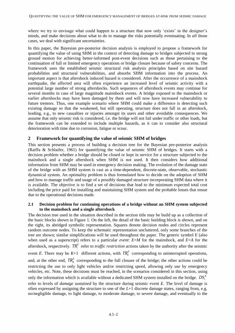
2.1 Decision problem for continuing operations of a bridge without an SHM system subjected
to the mainshock and a single aftershock
The decision tree used in the situation described in the section title may be build up as a collection of
the basic blocks shown in Figure 1. On the left, the detail of the basic building block is shown, and on
the right, its abridged symbolic representation. Squares denote decision nodes and circles represent
random outcome nodes. To keep the schematic representation uncluttered, only some branches of the
tree are shown; similar simplifications will be used throughout the paper. The generic symbol E (also
when used as a superscript) refers to a particular event: E=M for the mainshock, and E=A for the
aftershock, respectively. E
iTR refer to traffic restriction actions taken by the authority after the seismic
event E. There may be K+1 different actions, with 0
ETR corresponding to uninterrupted operations,
and, at the other end, E
KTR corresponding to the full closure of the bridge; the other actions could be
restricting the use to only light vehicles and/or restricting speed, allowing only use by emergency
vehicles, etc. Note, these decisions must be reached, in the scenarios considered in this section, using
only the information which is available without a dedicated SHM system installed on the bridge. E
iDS
refer to levels of damage sustained by the structure during seismic event E. The level of damage is
often expressed by assigning the structure to one of the L+1 discrete damage states, ranging from, e.g.
no/negligible damage, to light damage, to moderate damage, to severe damage, and eventually to the

The Value of Structural Health Monitoring for the
reliable Bridge Management
Zagreb 2-3 March 2017
4.5–3
total collapse. Alongside the different levels of damage, shown are the probabilities of their
occurrence, E
DSiP .
TRE0
...
...
DSE0 (P
EDS0)
...
...
TRE1
TREK
DSEL (P
EDSL)
DSE1 (P
MDS1)
= E: TRE(0:K), DSE(0:L), PEDS(0:L)
Fig. 1. Basic building block of decision tree to manage bridge usage
The full decision tree for continuing operations of a bridge without an SHM systems subjected to the
mainshock and a single aftershock is shown in Figure 2. Here, in the building blocks for the aftershock
events (denoted by symbol A), the probabilities |
|i j
A M
DS DSP of bridge sustaining a given level of damage,
DSi in the aftershock are conditional on the level of damage, DSj sustained in the mainshock, i.e. they
are transition probabilities. That in fact cast our problem as a dynamical, discrete-state stochastic
system. Without monitoring, the system is not observable, but once an SHM information is included,
which is explained in the following section, it will become observable. The system can be though as
time dependent, although this is now hidden in the occurrences of the mainshock and the aftershock.
This also expresses the fact that damage will accumulate over consecutive earthquakes. On the very
right of Figure 2 are consequences related to each combination of actions and random outcomes (states
of nature), , , , M M A A
ijkl i j k lC C TR DS TR DS , (i, k=0, 1, … K; j, l=0, 1, … L). For example, closing the
bridge altogether to traffic after the mainshock or the aftershock, when in fact it can be used without
restriction or perhaps at least for emergency services, will entail economic losses because of delays,
loss of service etc., and will possibly also mean delays in getting the injured to a hospital worsening
their condition. On the other hand, a bridge that is unsafe but allowed to operate may collapse leading
to additional economic losses or even casualties or new injuries.
M: TRM(0:K),DSM(0:L), PM
DS(0:L)
A: TRA(0:K),DSA(0:L),
PA|MDS(0:L)|DS0
A: TRA(0:K),DSA(0:L),
PA|MDS(0:L)|DS1
A: TRA(0:K),DSA(0:L),
PA|MDS(0:L)|DSL
...
...
C0000=C(TRM0,DSM
0,TRA0,DSA
0)
C0001=C(TRM0,DSM
0,TRA0,DSA
1)
CK0KL=C(TRMK,DSM
0,TRAK,DSA
L)
...
C0100=C(TRM0,DSM
1,TRA0,DSA
0)
C0101=C(TRM0,DSM
1,TRA0,DSA
1)
CK1KL=C(TRMK,DSM
1,TRAK,DSA
L)
...
C0L00=C(TRM0,DSM
L,TRA0,DSA
0)
C0L01=C(TRM0,DSM
L,TRA0,DSA
1)
CKLKL=C(TRMK,DSM
L,TRAK,DSA
L)
...
Fig. 2. Decision tree for continuing bridge operations for bridge without SHM system subjected to mainshock and aftershock

QUANTIFYING THE VALUE OF SHM FOR EMERGENCY MANAGEMENT OF BRIDGES AT-RISK FROM SEISMIC DAMAGE
4.5–4
The optimal pair of actions ,M A
optTR TR after the mainshock and the aftershock is the one that
minimizes the overall risk:
|0,1... 0,1...
, min minM A Mj l j
M A
ijklDS DS DSopt i K k KTR TR E E C
(1)
Here, E[] denotes the expected value operator.
2.2 Decision problem for continuing operations of a bridge with an SHM system subjected to
the mainshock and a single aftershock
To handle the scenario where an SHM system is to be adopted, another basic decision tree building
block is adopted as shown in Figure 3. Here, decisions to adopt a health monitoring system before
seismic event E are denoted as E
iHM . There may be N+1 such decisions, each corresponding to the
adoption of a particular SHM system or technology, with 0
EHE corresponding to the decision to not
adopt any. Note that the superscript E is still present as we envisage monitoring may be adopted before
the mainshock but alternatively only after the mainshock to monitor the structural performance and
damage in the aftershock of the bridge weakened in the mainshock (in which case it would be replaces
by superscript A). The cost of each system is indicated by CHMi, with CHM0=0. It should be noted that
for a fair assessment of the cost involved in monitoring a structure not only the cost of hardware
(capex) must be included but the whole life-cycle cost needs to be quantified (design, installation,
operational costs including maintenance, decommissioning, etc.), and the cost of data analysis and
integration of the SHM information into the emergency response process. E
iDD refer to damage
detected by the monitoring system. Again, it is envisaged that based on the SHM system indication,
the structural state will be mapped into one of the L+1 discrete detected damage states. The
probabilities of indication of the different levels of damage are indicated asE
DDiP . Note these
probabilities include correct as well as incorrect detected damage state classifications with respect to
the actual damage states the structure will find itself in.
HME0
... ...
DDE0 (P
EDD0)
...
HME1
DDEL (P
EDDL)
DDE1 (P
MDD1) =
HMEN
E: HME(0:N), DDE(0:L), PEDD(0:L)
dummy node
CHM1
CHMN
CHM0=0
Fig. 3. Basic building block of decision tree for SHM system adoption
With the newly introduced additional building block, we can now formulate the full decision tree for
adoption of an SHM system. It is shown in Figure 4. The consequences at the far-right end,
, , , , , , , M M M M A A A A
ijklmnpr i j k l m n p rC C HM DD TR DS HM DD TR DS , (i, m=0, 1, … N; j, l, n, r=0, 1, … L; k,
p=0, 1, … K), depend now also on the additional decisions to adopt or not an SHM system, and if so
which, and random outcomes include damage detection alerts issued by the SHM system. As one
moves from left to right, the probabilities of each damage state being indicated or actually sustained
depend on the entire history of preceding decisions and random outcomes.

The Value of Structural Health Monitoring for the
reliable Bridge Management
Zagreb 2-3 March 2017
4.5–5
M: HMM(0:N),DDM(0:L), PM
DD(0:L)
M: TRM(0:K),DSM(0:L),
PM|HMMDS(0:L)|DD0
M: TRM(0:K),DSM(0:L),
PM|HMMDS(0:L)|DD1
M: TRM(0:K),DSM(0:L),
PM|HMMDS(0:L)|DDL
...
A: HMA(0:N),DDA(0:L),
PA|M|HMMDD(0:L)|DS0|DD0
A: HMA(0:N),DDA(0:L),
PA|M|HMMDD(0:L)|DS1|DD0
A: HMA(0:N),DDA(0:L),
PA|M|HMMDD(0:L)|DSL|DD0
...
A: TRA(0:K),DSA(0:L),
PA|HMA|M|HMMDS(0:L)|DD0|DS0|DD0
A: TRA(0:K),DSA(0:L),
PA|HMA|M|HMMDS(0:L)|DD1|DS0|DD0
A: TRA(0:K),DSA(0:L),
PA|HMA|M|HMMDS(0:L)|DDL|DS0|DD0
...
C00000000=C(HMM0,DDM
0,TRM0,DSM
0,HMA0,DDA
0,TRA0,DSA
0)
C000000001=C(HMM0,DDM
0,TRM0,DSM
0,HMA0,DDA
0,TRA0,DSA
1)
CN000N0KL=C(HMMN,DDM
0,TRM0,DSM
0,HMAN,DDA
0,TRAK,DSA
L)
...
Fig. 4. Decision tree for continuing bridge operations for bridge with SHM system subjected to mainshock and aftershock
The conditional probabilities PDSi|DDj of damage state DSi having actually been sustained when damage
state DDj has been indicated by the SHM system appearing in the decision tree may be found from the
state probabilities i
M
DSP and state transition probabilities |
|i j
A M
DS DSP (i, j=0,1,…L), and the probabilities
|j iDD DSP of correct/incorrect indications of damage states by the monitoring system, for example:
|
0
j i j i
LM M M
DD DS DD DS
i
P P P (2)
||
| M
i j i
i j
j
M M
DS DD DSM HM
DS DD M
DD
P PP
P (3)
The optimal set of actions , , ,M M A A
optHM TR HM TR is the one that minimizes the overall risk:
| | | | | |0,1... 0,1... 0,1... 0,1...
, , , min min min minM M M A M M A A M Mj l j n l j r n l j
M M A A
ijklmnprDD DS DD DD DS DD DS DD DS DDopt i N k K m N p KHM TR HM TR E E E E C
(4)
3. Bridge seismic risk modelling: hazard and fragility for
The probability i
E
DSP of a bridge sustaining damage state DSi when subjected to an earthquake during
its expected service life is a critical parameter in the proposed framework (see Figure 1). This
probability is a function of hazard at the site and fragility of the bridge. The probability i
E
DSP can be
estimated using the following expression:
1
0
d ( )
di
E IM
DS i iD IM D IM
s x
sP F d x F d x dx
s
(5)
In the expression above, FD|IM(.|.) is the cumulative conditional probability distribution of peak
demand, D, imposed on the bridge conditioned on the intensity measure, IM, of strong ground motion
at the site. Variables di and di+1 are the demand levels (e.g. strains, curvatures, displacements)
corresponding to the onset of damage states DSi and DSi+1, respectively. The expression |dIM/ds| is the
absolute value of the derivative of the estimated seismic hazard IM. Typical IM parameters are
pseudo-spectral acceleration of the equivalent damped single-degree-of-freedom system, Sa(T), peak
ground velocity, PGV, and peak ground acceleration, PGA. IM establishes the connection between the
hazard and the vulnerability. Therefore, it is critical to adopt a measure that can effectively capture the
seismic behavior of the bridge and can be probabilistically estimated with an acceptable level of

QUANTIFYING THE VALUE OF SHM FOR EMERGENCY MANAGEMENT OF BRIDGES AT-RISK FROM SEISMIC DAMAGE
4.5–6
uncertainty. Benefits and limitations of alternative IMs are discussed by Weatherhill et al. (2011). In
the following, potential strategies for estimating the seismic hazard, IM, and the fragility, FD|IM, will be
presented.
The seismic hazard at the site of the bridge can be estimated by performing a probabilistic seismic
hazard assessment (PSHA) as proposed by Cornell (1968). In PSHA, the rate, IM, at which the strong
motion intensity, IM, at the site is expected to exceed a specific level, s, within a fixed time is
assessed. The rate IM is evaluated using the following expression:
max max
min1 0
,s
m rn
IM i MR Mi m
s P IM s m r f r m f m dm dr
(6)
where ns is the number of seismic sources that are expected to induce significant shaking at the site, i
is the rate of earthquakes that occur at the i-th source and which have magnitudes within the range
bounded by the minimum magnitude, mmin, and the maximum magnitude, mmax. The term P[IM >s| m,
r] is the conditional probability of shaking intensity IM at the site exceeding level s, given that the site
is excited by an earthquake of magnitude m and with a rupture plane that lies at a distance r from the
site. This probability is estimated using ground motion prediction equations which aim at capturing the
expected attenuation or amplification of the seismic waves which propagate along the path from the
source to the site (Kramer, 1996). Probability density fM(m) is equal to the relative likelihood of
magnitudes of earthquakes that occur within considered time being equal to m. Likewise, fR|M(r|m) is
the conditional probability of the source-to-site distance being equal to r for an earthquake with
magnitude m.
In the proposed framework, seismic hazards associated with two different types of earthquakes are
considered, namely the mainshock and the aftershock earthquakes. Large magnitude earthquakes are
often preceded and succeeded by smaller magnitude events that occur at the proximity of each other
and within a short period. An entire sequence of earthquakes is referred to as a cluster. Within a
cluster, the event with the greatest magnitude is named the mainshock and all the following
earthquakes are called aftershocks. Existing earthquake catalogs suggest that mainshock earthquakes
often occur at a relatively constant rate at seismic source zones. Accordingly, these events are
typically modelled as a homogeneous Poisson processes in the conventional PSHA. Hence, the
probability i
M
DSP - related to the mainshock - can be obtained using IM obtained from Equation (6) and
considering structural vulnerability or fragility.
The aftershock earthquakes occur at a rate that decays with time elapsed since the mainshock. The
characteristics of this decay were first systematically investigated by Omori (1894). Even today,
Omori’s model is frequently used for modeling the decaying of rate of aftershocks. Since the rate of
aftershocks is not constant over time, the aftershock events are modelled as a non-homogenous
Poisson processes in the PSHA. Yeo and Cornell (2009) proposed a modified version of PSHA that
considers the time dependent decay of the rate of events. Recently, Müderissoglu and Yazgan (2017)
developed a modified version of this approach, which enables making use of mainshock strong motion
recordings in updating the uncertainty associated with the expected attenuation of the aftershock
induced shaking. This updating results in changing of the conditional likelihood P[IM>s|m,r] in
Equation (5). In case of bridges designed and constructed according to modern seismic codes, the
primary source of uncertainty associated with the expected performance is that due to uncertainty of
the estimated hazard. Therefore, such an updating of the uncertainty associated with the hazard
estimate would often lead to a considerable change in the predicted seismic performance.
The aftershock hazard assessment method developed by Müderrisoglu and Yazgan (2017) is especially
suitable for bridges which have free-field strong motion recoding instruments. In the context of the
framework proposed here, such instrumentation may be conceived as a part of the monitoring system.
Using the method, the ground motion recorded by the free-field sensor can be utilized to revise the
uncertainties associated with the expected level of attenuation. Thus, the aftershock hazard conditional
on the recorded mainshock motion can be obtained. When compared to the case with no
instrumentation, this conditional hazard estimate would result in higher or lower exceedance rates.

The Value of Structural Health Monitoring for the
reliable Bridge Management
Zagreb 2-3 March 2017
4.5–7
This difference depends on the motion intensity level registered during the mainshock event. The
aftershock damage probabilities, |
|j i
A M
DS DSP , corresponding to the decision tree branch in Figure 4 related
to not adopting any monitoring system (i.e. MHM 0) may be evaluated using the conventional
aftershock hazard assessment approach by Yeo and Cornell (2002). On the other hand, the
probabilities |
|j i
A M
DS DSP corresponding to the branches related to adopting a monitoring system (i.e.
M
iHM , i=1,2,…N) can be evaluated by substituting the IM estimates obtained using the method by
Müderrisoglu and Yazgan (2017) into Equation (5).
The conditional probability of a bridge sustaining damage state DSi when subjected to a given level of
shaking intensity is referred to as the seismic fragility. This conditional probability is represented by
the term FD|IM(.|.) in Equation (5). There exists a large variety of methods proposed for assessing
seismic fragility of structures (Porter, 2003). In the proposed framework, an approach that can be
applied to individual structures is needed. Moreover, the approach should enable rational consideration
of various sources of uncertainty that have significant impact on the estimated likelihood FD|IM. Based
on these constraints, the ‘analytical approach’ for fragility modeling is particularly suited to the
framework presented here.
In the analytical fragility modeling approach, a basis numerical model of the bridge is developed for
seismic response analysis. The uncertainties associated with the model are assessed and probability
distributions are established to capture their random variability. Typically, the existing
recommendations (e.g. JCSS, 2001) are utilized for this purpose. A set of alternative models are
generated using these probability distributions. Subsequently, a suite of strong ground motion records
is established. The records are selected to capture with a required accuracy the mean value and
dispersion of the seismic response of the bridge that will be exhibited when it is subjected to the
expected seismic events during its service life (Kalkan & Chopra, 2010). For each randomly generated
model with a ground motion, incremental dynamic analysis (Vamvatsikos & Cornell, 2002) can be
performed. In this process, the response of the bridge to the specific ground motion is simulated by
gradually scaling up the ground motion to different IM levels. The record is scaled to the level when
the computed demand becomes just equal to the threshold di associated with the onset of damage state
DSi. The intensity level dix that correspond to this threshold is determined for all model realization
and ground motion record pairs. Subsequently, the fragility is evaluated as follows:
2
1 1
1 1, where and
1
m mn n
i
i i di i di iD IMj ji m m
xF d x x j x j
n n
(7)
In the equation above, (.) is the standard normal distribution function, i and i are the mean and
standard deviation of the IM levels that correspond to the onset of DSi, and nm is the total number of
model and record pairs. The fragility estimates related to both damage state DSi and the next more
severe one DSi+1 needs to be substituted into Equation (5) in order to evaluate the probability i
M
DSP of
the bridge sustaining damage state DSi. The damage probability i
M
DSP is obtained by considering the
response of the intact bridge to the mainshock event.
The likelihood |
|i j
A M
DS DSP of the mainshock induced damage grade DSi progressing to a higher grade DSj
because of aftershock induced shaking is needed in the proposed framework. Evaluation of the
conditional probability |
|i j
A M
DS DSP for a bridge is a more challenging task compared to evaluation of i
M
DSP .
In this evaluation, the fragility analysis needs to be performed using a damaged bridge model rather
than an intact one. Specifically, the damage imposed on the model should be of grade DSi. The actual
mainshock motion that will impose this damage during the expected service life is not available at the
time of assessment. The damage grade is a global measure of damage while the actual seismic
response is sensitive to all local damages within critical locations combined. Thus, different ground

QUANTIFYING THE VALUE OF SHM FOR EMERGENCY MANAGEMENT OF BRIDGES AT-RISK FROM SEISMIC DAMAGE
4.5–8
motion records may damage critical zones of the bridge to varying extents as they impose the same
global damage state DSi. In the evaluation of conditional likelihood |
|i j
A M
DS DSP , this record-to-record
variability of mainshock motions that impose the same DSi grade needs to be considered. One strategy
to achieve this is to establish a set of mainshock motions and identify the scaling factors for each of
these motions that correspond to the onset of damage state DSi. Subsequently, aftershock fragility
analysis is performed by simulating the response of each randomly generated structural analysis model
to sequences of ground excitations. This sequences should consist of the mainshock shaking that
imposes damage state DSi followed by an aftershock excitation (Ryu et al., 2011). The specific
aftershock shaking intensity level x’dj that corresponds to the onset of damage state DSj, is identified
by repeating this analysis for a range of aftershock scaling factors. In this analysis, the polarity of
aftershock excitation should be randomized as recommended by Ryu et al. (2011). It should be born in
mind that the process entails considerable computational effort. To reduce this effort, an approach
based on nonlinear regression recommended by Alessandri et al. (2013) may be adopted.
After the intensity levels x’dj are identified for all the mainshock-aftershock sequences, Equation (7)
may be utilized to establish the aftershock fragility of the bridge. In this case the resulting fragility
FD|IM;DSi(dj|x;DSi) is conditioned on the mainshock induced damage state DSi. The required conditional
probabilities |
|i j
A M
DS DSP can be obtained by substituting FD|IM;DSi(dj|x;DSi) into Equation (5).
4. Probability of damage state classification and integration of SHM data into bridge reliability
assessment
Quantifying the value of SHM via the Bayesian pre-posterior analysis as described in this paper and
integration of SHM data into bridge reliability assessment requires probabilities |i j
E
DD DSP of
classification of structural states based on the indication from the SHM system. These can generally be
found from probability distribution functions of a damage indicator corresponding to the different
actual damage states (Omenzetter et al. 2016). These probability distributions will be dependent on the
particular SHM system adopted. Here, we need to consider the whole process of SHM data collection
and processing which output a damage state indicator. There are a number of challenges at this point
as discussed below.
The various structural damage states are known to correlate better with measures related to structural
displacements or rotations and associated ductilities, the latter particularly relevant for modern
structures designed for seismic regions. For example, Table 1 (Banerjee & Shinozuka, 2008) shows
classification of damage into several states depending on the rotational ductility demands. Yet
measuring displacements or rotations in-situ for large structures presents a considerable practical
challenge, mostly because a fixed reference base is difficult to find for contact measurement
technologies, such as linear variable displacement transducers. Non-contact devices will often require
a stable base too, which may not be easily available in seismic monitoring, and unobstructed line of
sight, which is often unavailable due to vegetation, complex terrain or in densely built-up environs.
The global positioning system does not yet offer accuracies required in our context. Strain gauges, and
other types of attachable sensors for that matter, will not survive in the areas of large deformations –
where we would ideally like them to be placed - because of cracking and spalling. On the other hand,
the type of measurements that are more readily available, notably accelerations, do not yield features
that readily map quantitatively into structural damage states. Double integration of acceleration time
histories to obtain displacements is fraught with drifts. Any practically useful framework for
quantifying the value of seismic SHM must recognize such practicalities.

The Value of Structural Health Monitoring for the
reliable Bridge Management
Zagreb 2-3 March 2017
4.5–9
Table 1. Damage states and corresponding rotational ductility demands (adopted from Banerjee & Shinozuka, 2008)
Damage state Rotational ductility demand
None <1
Negligible 1-1.52
Minor 1.52-3.10
Moderate 3.10-5.72
Major 5.72-8.34
Collapse >8.34
A damage detection/classification and future reliability prediction solution that uses acceleration
measurements combined with structural model updating and nonlinear time history analysis to
establish the probabilities of correct and incorrect classification of structural state based on the
indication from the SHM system is proposed here by extending the earlier work of Soyoz and his
collaborators (Soyoz et al., 2010, Kaynardag & Soyoz, 2015; Özer & Soyoz, 2015). The approach
adopted comprises the following steps:
A nonlinear finite element (FE) model of the bridges is formulated. This model may also
include effects such as soil-structure interaction if deemed important.
When acceleration data captured by and SHM system becomes available it is used as input to
a system identification algorithm to determine modal properties (natural frequencies, damping
ratios and mode shapes). Note the type of data applicable for this step is from low level
excitations such that the linear response regime prevails. It may be an output-only system
identification, but if ground motion sensors are installed next to the bridge and/or on its
foundations as part of the SHM system, input-output methods can be adopted that can improve
the reliability of results. Enhanced system identification approaches may include considering
environmental and operational effects on the responses, such as temperature or presence of
vehicles on the deck.
The FE model initial stiffness is calibrated (updated) against the identified modal parameters.
Note because of the linearity limitation above other model parameters that govern the
nonlinear part of the response cannot be inferred directly using this approach.
The updated model is run for nonlinear time history analyses to identify the fragility of the
calibrated model. In these analyses, the damage states are established based on, e.g. ductility
of the numerically simulated response (Table 1).
Some sources of uncertainties propagating into potential misclassification errors and affecting |i j
E
DD DSP ,
such as the level of noise in acceleration sensor measurements, can be garnered from laboratory trials
and previous field applications. In a similar way, uncertainties in modal system identification results
(Chen et al., 2014; Chen et al., 2015) and numerical model updating procedures (Shabbir &
Omenzetter, 2016) can be assessed. A ‘trial’ monitoring system can be installed to gather more site-
specific data and reduce uncertainties, but a decision to do so should then be assessed for cost-benefit
within the proposed decision making framework. However, beyond those the methodology will have
very limited access to experimental validation data. Note we try to make inferences about the
performance of an SHM system before we actually deploy it on the structure, thus have no ‘hard’
measured data. Since large structures such as bridges are unique, even available data or experience
from ‘similar’ structures will have limitations. In any case, there is very little monitoring data
available thus far from bridges that actually sustained seismic damage. Circumventing this major
challenge will require relying on extensive probabilistic numerical simulations, where the given
structural system with all expected uncertainties will be simulated for random combinations of
structural properties and ground motion inputs to determine its ‘virtual’ acceleration responses. These
responses will then be fed into the bullet-point procedure outlined above to obtain the detected damage
state DDi results for each response simulation. Afterwards, the resulting detected damage states will be
compared to the ‘actual’ damage states DSi obtained directly from the structural model obtained using
ductility thresholds such as those in Table 1. It is clear that many an assumption will be made in this
QUANTIFYING THE VALUE OF SHM FOR EMERGENCY MANAGEMENT OF BRIDGES AT-RISK FROM SEISMIC DAMAGE
4.5–10
approach, and that formidable computational effort must be reckoned with in the pre-posterior analysis
stage to map the measurements to failure probabilities. However, it should also be recognized that the
actual operation of the damage classification system does not necessarily entail running the time
consuming nonlinear time history analyses. Based on such analyses during the decision-making stage,
relationships, e.g. utilising artificial neural networks, can be built between the identified stiffness loss,
or even just recorded ground and response intensity measures like PGA and peak structural response
acceleration, and failure probabilities for quick, near real-time estimation of the associated risks (de
Lautour & Omenzetter, 2009).
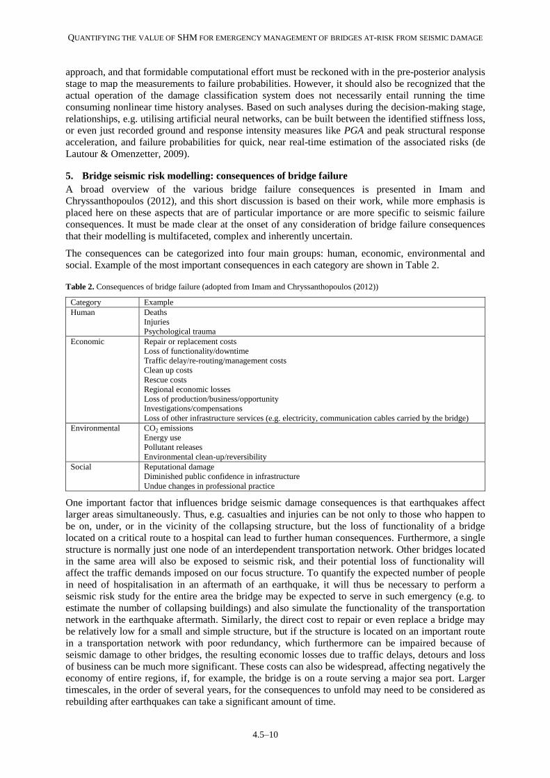
5. Bridge seismic risk modelling: consequences of bridge failure
A broad overview of the various bridge failure consequences is presented in Imam and
Chryssanthopoulos (2012), and this short discussion is based on their work, while more emphasis is
placed here on these aspects that are of particular importance or are more specific to seismic failure
consequences. It must be made clear at the onset of any consideration of bridge failure consequences
that their modelling is multifaceted, complex and inherently uncertain.
The consequences can be categorized into four main groups: human, economic, environmental and
social. Example of the most important consequences in each category are shown in Table 2.
Table 2. Consequences of bridge failure (adopted from Imam and Chryssanthopoulos (2012))
Category Example
Human Deaths
Injuries
Psychological trauma
Economic Repair or replacement costs
Loss of functionality/downtime
Traffic delay/re-routing/management costs
Clean up costs
Rescue costs
Regional economic losses
Loss of production/business/opportunity
Investigations/compensations
Loss of other infrastructure services (e.g. electricity, communication cables carried by the bridge)
Environmental CO2 emissions
Energy use
Pollutant releases
Environmental clean-up/reversibility
Social Reputational damage
Diminished public confidence in infrastructure
Undue changes in professional practice
One important factor that influences bridge seismic damage consequences is that earthquakes affect
larger areas simultaneously. Thus, e.g. casualties and injuries can be not only to those who happen to
be on, under, or in the vicinity of the collapsing structure, but the loss of functionality of a bridge
located on a critical route to a hospital can lead to further human consequences. Furthermore, a single
structure is normally just one node of an interdependent transportation network. Other bridges located
in the same area will also be exposed to seismic risk, and their potential loss of functionality will
affect the traffic demands imposed on our focus structure. To quantify the expected number of people
in need of hospitalisation in an aftermath of an earthquake, it will thus be necessary to perform a
seismic risk study for the entire area the bridge may be expected to serve in such emergency (e.g. to
estimate the number of collapsing buildings) and also simulate the functionality of the transportation
network in the earthquake aftermath. Similarly, the direct cost to repair or even replace a bridge may
be relatively low for a small and simple structure, but if the structure is located on an important route
in a transportation network with poor redundancy, which furthermore can be impaired because of
seismic damage to other bridges, the resulting economic losses due to traffic delays, detours and loss
of business can be much more significant. These costs can also be widespread, affecting negatively the
economy of entire regions, if, for example, the bridge is on a route serving a major sea port. Larger
timescales, in the order of several years, for the consequences to unfold may need to be considered as
rebuilding after earthquakes can take a significant amount of time.

The Value of Structural Health Monitoring for the
reliable Bridge Management
Zagreb 2-3 March 2017
4.5–11
6. Conclusions
We have outlined a framework for quantifying the value of information from SHM technology
installed on a bridge. The general case we consider is that of a bridge structure that may sustain
damage in the mainshock and further progressing damage in an aftershock. The value of SHM
information is computed using the Bayesian pre-posterior approach to decision making. The evolution
of the damage state of the bridge with an SHM system is conceptualised as a time-dependent,
stochastic, discrete-state, observable dynamical system. Optimal decisions whether to adopt SHM and
how to restrict traffic on a potentially damaged structure is formulated to minimise the expected total
cost or risk. The paper then discusses how to estimate the bridge damage probability through
stochastic seismic hazard and fragility analysis, and how to update these probabilities using SHM data
through an approach that combines modal system identification, structural model updating and
nonlinear time history simulations. Finally, a brief overview of quantifying bridge failure
consequences is included.
Acknowledgements
Piotr Omenzetter works at the Lloyd’s Register Foundation Centre for Safety and Reliability Engineering at the
University of Aberdeen. The Foundation helps to protect life and property by supporting engineering-related
education, public engagement and the application of research. The COST Action TU1402 on Quantifying the
Value of Structural Health Monitoring is gratefully acknowledged for networking support.
References
Alessandri, S, Giannini R and Paolacci F (2011) Aftershock risk assessment and the decision to open traffic on
bridges. Earthquake Engineering and Structural Dynamics, 42, 2255-2275.
Banerjee, S and Shinozuka, M (2008) Integration of empirical, analytical and experimental seismic damage data
in the quantification of bridge seismic damage states. Proceedings of the Concrete Bridge Conference
HPC — Safe, Affordable and Efficient.
Chen, G-W, Omenzetter, P and Beskhyroun, S (2015) A comparison of operational modal parameter
identification methods for a multi-span concrete motorway bridge. Proceedings of the 2015 New Zealand
Society for Earthquake Engineering Annual Conference, 1-8.
Chen, X, Omenzetter, P and Beskhyroun, S (2014) Assessment of a segmental post-tensioned box girder bridge
using ambient vibration testing. Proceedings of the 23rd
Australasian Conference on the Mechanics of
Structures and Materials, 1103-1108.
Cornell, A (1968) Engineering seismic risk analysis. Bulletin of the Seismological Society of America, 58(5),
1583-1606.
de Lautour, OR and Omenzetter, P (2009). Prediction of seismic-induced structural damage using artificial
neural networks. Engineering Structures, 31, 600-606.
Imam, BM and Chryssanthopoulos, MK (2012) Causes and consequences of metallic bridge failures. Structural
Engineering International, 22(1), 93-98.
JCSS – Joint Committee on Structural Safety (2001) Probabilistic model code 2001. http://www.jcss.ethz.ch.
Kaynardag, K and Soyoz, S (2015) Effect of identification on seismic performance assessment of a tall building.
Bulletin of Earthquake Engineering, 1–7.
Kalkan, E and Chopra, AK (2010) Practical guidelines to select and scale earthquake records for nonlinear
response history analysis of structures. Open-File Report 2010, US Geological Survey, Menlo Park,
California.
Kramer, SL (1996) Geotechnical earthquake engineering. Prentice Hall, Upper Saddle River, New Jersey.
Müderrisoglu, Z and Yazgan, U (2017) A new approach for aftershock hazard assessment that takes into account
mainshock demand. Proceedings of the 16th
World Conference on Earthquake Engineering, Santiago,
Chile, 1-12.

QUANTIFYING THE VALUE OF SHM FOR EMERGENCY MANAGEMENT OF BRIDGES AT-RISK FROM SEISMIC DAMAGE
4.5–12
Omenzetter, P, Limongelli, MP and Yazgan, U (2016) Quantifying the value of seismic monitoring for the
building owner. Proceedings of the 8th European Workshop on Structural Health Monitoring, Bilbao,
Spain, 1-10.
Omori, F (1894) On after-shocks of earthquakes. Journal of College of Science, Imperial University of Tokyo,
7(1), 111-200.
Özer, E and Soyoz, S (2015) Vibration-based damage detection and seismic performance assessment of bridges.
Earthquake Spectra, 31(1), 137–157.
Porter, KA (2003) Seismic vulnerability. In: Chen, W-F and Scawthorn, C, eds. Earthquake engineering
handbook. Raton, Florida, CRC Press.
Ryu, H, Luco, N, Uma, SR and Liel, AB (2011) Developing fragilities for mainshock-damaged structures
through incremental dynamic analysis. Proceedings of the 9th Pacific Conference on Earthquake
Engineering, Auckland, New Zealand, 1-8.
Raiffa, H and Schlaifer, R (1961) Applied statistical decision theory. Harvard University.
Shabbir, F and Omenzetter, P (2016) Model updating using genetic algorithms with sequential niche technique.
Engineering Structures, 120, 166-182.
Soyoz, S, Feng, MQ and Shinozuka, M (2010) Structural reliability estimation with vibration-based identified
parameters. Journal of Engineering Mechanics, 136(1), 100–106.
Vamvatsikos, D and Cornell, CA (2002) Incremental dynamic analysis. Earthquake Engineering and Structural
Dynamics, 31(3), 491-514.
Weatherhill, G, Crowley, H and Pinho, R (2011) Efficient intensity measure for components within a number of
infrastructures. SYNER-GR Project Report No D2.12, University of Pavia, Pavia, Italy.
Yeo, G and Cornell, A (2009) A probabilistic framework for quantification of aftershock ground-motion hazard
in California: Methodology and parametric study. Earthquake Engineering and Structural Dynamics, 38,
45-60.


