

Why did Rich Families Increase their Fertility? Inequality andMarketization of Child Care
FEDERAL RESERVE BANK OF ST. LOUISResearch Division
P.O. Box 442St. Louis, MO 63166
RESEARCH DIVISIONWorking Paper Series
Michael Bar,Moshe Hazan,
Oksana Leukhina,David Weiss
andHosny Zoabi
Working Paper 2018-022A https://doi.org/10.20955/wp.2018.022
September 2018
The views expressed are those of the individual authors and do not necessarily reflect official positions of the FederalReserve Bank of St. Louis, the Federal Reserve System, or the Board of Governors.
Federal Reserve Bank of St. Louis Working Papers are preliminary materials circulated to stimulate discussion andcritical comment. References in publications to Federal Reserve Bank of St. Louis Working Papers (other than anacknowledgment that the writer has had access to unpublished material) should be cleared with the author or authors.

Why did Rich Families Increase their Fertility?Inequality and Marketization of Child Care∗
Michael Bar† Moshe Hazan‡ Oksana Leukhina§
David Weiss¶ Hosny Zoabi‖
September 25, 2018
Abstract
A negative relationship between income and fertility has persisted for so long that its
existence is often taken for granted. One economic theory builds on this relationship and
argues that rising inequality leads to greater differential fertility between rich and poor.
We show that the relationship between income and fertility has flattened between 1980
and 2010 in the US, a time of increasing inequality, as high income families increased
their fertility. These facts challenge the standard theory. We propose that marketization
of parental time costs can explain the changing relationship between income and fertility.
We show this result both theoretically and quantitatively, after disciplining the model on
US data. We explore implications of changing differential fertility for aggregate human
capital. Additionally, policies, such as the minimum wage, that affect the cost of marke-
tization, have a negative effect on the fertility and labor supply of high income women.
We end by discussing the insights of this theory to the economics of marital sorting.
Keywords: Income Inequality, Marketization, Differential Fertility, Human Capi-
tal, Minimum Wage.
JEL Classification Numbers: E24, J13, J24, J31, J38.
∗We thank three anonymous referees, Paul Beaudry, Alma Cohen, Mariacristina De Nardi, Matthias Doepke, AxelleFerriere, Oded Galor, Jeremy Greenwood, Nezih Guner, Lutz Hendricks, Yishay Maoz, Marla Ripoll, Analia Schlosser,Itay Saporta-Eksten, Tom Vogl, David Weil, Alan Weiss, Yaniv Yedid-Levi and seminar participants in various seminars,workshops, and conferences for helpful comments. We thank Sergei Filiasov and Yannay Shanan for excellent researchassistance. Moshe Hazan acknowledges financial support provided by the Israel Science Foundation and the Falk Institutefor the quantitative part of the paper. Hosny Zoabi acknowledges the financial support of the Russian Science Foundation,grant #18-18-00466 for supporting the theoretical part of the paper. This paper was previously circulated under the title“Is The Market Pronatalist? Inequality, Differential Fertility, and Growth Revisited.”
†San Francisco State University. E-mail: [email protected]‡Tel-Aviv University and CEPR. E-mail: [email protected]§McMaster University. E-mail: [email protected]¶Tel Aviv University. E-mail: [email protected]‖New Economic School, 45 Skolkovskoe shosse, Moscow, Russia. E-mail: [email protected]
1 Introduction
A negative relationship between income and fertility has persisted for so long
that its existence is often taken for granted in the literature (Jones & Tertilt 2008).
This relationship has been typically explained by either the tradeoff between the
quantity and quality of children, the opportunity cost of parental time, or both.
Some of the many examples include Becker & Lewis (1973), Galor & Weil (1996),
Galor & Weil (2000), and Doepke (2004). These mechanisms have led researchers
to conclude that rising inequality would lead to a larger differential fertility be-
tween poor and rich households (de la Croix & Doepke 2003, Moav 2005).1
However, as recent decades have seen a dramatic rise in income inequality in
the US, the relationship between income (or education) and fertility has flattened
as high income families increased their fertility challenging the conventional wis-
dom.2 We argue that the ability to substitute parental time by purchasing babysit-
ters, housekeepers, and prepared food, lessens children’s opportunity cost. As
inequality grows, the cost of marketization of the time cost of children for the
rich shrinks relative to their income, allowing them to have more kids without
sacrificing time and careers.
In this paper, we show that changes in inequality, and the associated decline in
the price of market substitutes for parents’ time with children, can quantitatively
account for much of the changing relationship between income and fertility over
time. We explore quantitatively and empirically the implications of our findings
for aggregate human capital accumulation and policy (minimum wage).
Our point of departure is the standard model of fertility and educational invest-
ment in children, as in Galor & Weil (2000), applied to the case of inequality as
in de la Croix & Doepke (2003) and Moav (2005). This model features both a
quantity-quality tradeoff with respect to children as well as an opportunity cost
of parental time in childcare. We analyze this model under the assumption that
1 Galor & Moav (2002) argue that the opposite is true before the demographic transition. Re-latedly, Vogl (2016) indeed finds that the income-fertility gradient was positive in less developedcountries before they experienced the demographic transition.
2See Autor, Katz & Kearney (2008) and Heathcote, Perri & Violante (2010) regarding risinginequality and Hazan & Zoabi (2015) regarding changing fertility patterns.
1

the cost of children can be marketized. We show that this one assumption is
crucial for understanding the effects of inequality on differential fertility.
Turning towards our quantitative analysis, we calibrate the model to the US in
1980, when fertility and income had a negative relationship. We discipline the
model by matching the salient features of cross-sectional US data. Namely, we
match the income profiles of fertility rates, mother’s labor supply, marketization
expenditures, and college attainment rates.3 The model successfully fits the em-
pirical targets with 8 parameters chosen to match 40 moments.
We then feed into the calibrated model the observed cross-sectional wages for
2010 and a price decline of home production substitutes. The model predicts
the 2010 relationships between income and fertility and between income and
mother’s time at home. In the model (data), the fertility of the top two deciles
increases by 43.5% (40%) between 1980 and 2010. Our measure of differential
fertility, which compares the average fertility of the top two deciles to that of the
second decile, increases by 41% (38.5%). An alternative measure of differential
fertility, comparing the fertility of the top half and bottom half of the income
distribution, increases by 24.4% (18.6%). All of these results are untargeted.
Decomposing the mechanisms at work, we find that it is the change in the price
of market substitutes relative to parental income, rather than the general income
effect, that is the main driver behind our findings. Furthermore, this result de-
pends critically on increasing inequality in parental wages. Our results imply
that a naïve modeler, working in 1980 under the view of the standard literature,
which ignores marketization, would have predicted a significant decline in fer-
tility among high income households over time if she had been given perfect
foresight over the evolution of income distributions.
One implication of our theory is that rising inequality increases aggregate human
capital, and thus growth. This is due to the fact that the rich tend to provide more
human capital to their children, as represented by college graduation rates. Thus,
as inequality increases, the average human capital of the next generation grows
as relatively more kids are born to richer families.
3We measure marketization expenditures as the relative expenditures on childcare, as calcu-lated from the Survey of Income and Program Participation (SIPP). See Appendix A for details.
2
Turning towards policy implications, according to our theory, anything affecting
the price of marketization should have an indirect effect on the labor supply and
fertility, especially of high income women. One prevalent policy that may af-
fect the price of marketization is the minimum wage. We show empirically that
the minimum wage level indeed has a large pass-through effect on wages in the
home production substitute (HPS) sector.4 Evaluating this effect in the context of
the calibrated model allows us to quantify the impact of minimum wage laws on
fertility and labor supply of high income women. This analysis is presented in
Section 5.
Accordingly, we show that a disproportionately large number of workers in the
HPS sector receive the minimum wage. Using cross state time series variation
in the minimum wage from 1980 to 2010, we show that the minimum wage has
a statistically significant and economically meaningful effect of about 58 cents
increase in HPS sector wages for every dollar increase of the state minimum wage.
We take an instrumental variables approach, as in Baskaya & Rubinstein (2012),
as OLS may be biased as states tend to raise the minimum wage during good
economic times.
We employ this estimated effect to perform a policy experiment, using the model
to measure the effects of raising the minimum wage to $15/hour, as per Bernie
Sanders, on the labor supply and fertility of high income women.5 These women
reduce their labor supply and fertility as marketizing becomes more difficult.6
We confirm the model prediction with respect to labor supply by estimating the
empirical elasticity of the labor supply of high income women with respect to
the minimum wage. We do so using cross state time series variation in the mini-
mum wage from 1980 to 2010 and the instrumental variable approach discussed
above. The empirical elasticity is also negative, but quantitatively larger in abso-
lute value than that of the model.
We conclude by discussing that explicit modeling of outsourcing of home
4We define these sectors as in Mazzolari & Ragusa (2013).5See http://berniesanders. om/issues/a-living-wage6Doepke & Kindermann (2016) argue that policies that lower the childcare burden on mothers
are significantly more effective at increasing fertility as compared to general child subsidies. Weargue that the minimum wage is a policy that increases the childcare burden on mothers, andhence decreases fertility.
3

production can also help us understand additional aspects of marital sorting
(Greenwood, Guner & Vandenbroucke 2017).
Hazan & Zoabi (2015) was the first paper to document the flattening of the fer-
tility profile by mother’s education, due to rising fertility rates among highly
educated women. They qualitatively study a similar model to the one presented
here to show theoretically the role of marketization. Furthermore, they exploit
cross-state variation in wages and find that the wages of childcare workers, rela-
tive to mothers’ wages, are negatively correlated with the propensity to have an
extra child. This reduced-form evidence supports the quantitative analysis done
in this paper. However, we differ in several critical ways. First, we document
the flattening of the fertility-income profile. Second, we quantitatively evaluate
the role of rising wage inequality and decreasing prices of home production sub-
stitutes, through the mechanism of marketization, in explaining this pattern. Fi-
nally, we examine theoretically and quantitatively the implications of inequality
and marketization for human capital accumulation and minimum wage policy.
This paper is related to a large literature on motherhood and labor supply. At-
tanasio, Low & Sanchez-Marcos (2008) builds a life cycle model of fertility and
labor force participation. They argue that reductions in child care costs can quan-
titatively account for the increase in labor supply of young mothers. Furtado
(2016) finds that an increase in unskilled migration lowers wages in the child
care services sector, and increases both fertility and labor supply.7 Interestingly,
she finds that native women with a graduate degree increase their labor supply
and fertility much more than native women with just a college degree. Similarly,
Cortés & Tessada (2011) exploit cross-city variation in immigration concentration,
and show that an increase in low-skilled immigration increases labor supply, of
women in the top quartile of the wage distribution.8 These women reduce time
spent on housework and purchase more services as substitutes. Interestingly,
Cortés & Pan (Forthcoming) show that increased marketization of household
7Notice that this tackles inequality from another direction. Rather than focus on a rise ininequality due to rising wages among high income households, she is studying an increase in thesupply of low wage workers. Our mechanism is agnostic as to the source of rising inequality.
8Using data from Hong Kong, Cortés & Pan (2013) show that the ability to hire foreign workersas live-in help increases labor force participation of mothers. They argue that child care costreduction through immigration is a market alternative to child care subsidies.
4

work allows women both to enter occupations that demand high levels of ef-
fort, and lowers the earnings gap in those occupations. While the importance of
marketization of home production has been widely recognized (e.g. Greenwood,
Seshadri & Vandenbroucke 2005, Greenwood, Seshadri & Yorukoglu 2005), the
consequences of rising inequality on differential fertility in the presence of the
possibility to outsource home production have not been widely studied.9
We continue as follows. Section 2 presents our motivating evidence. Section 3
describes the theoretical framework of our analysis. Section 4 provides details
on the parameterization of the model, along with quantitative results. Section 5
analyzes the effects of the minimum wage on labor supply and fertility through
the lens of the calibrated model. Section 6 discusses implications of marketization
on the literatures on marital sorting. We conclude in Section 7.
2 Motivating Evidence
In this section, we describe our motivating evidence. We first show data on cross-
sectional fertility changes and inequality. We then use cross-state variation in
9 The literature on women’s labor force participation is too vast to summarize here. However,a few papers showing how women’s labor supply is related to structural transformation andtaxes are worth noting, as they illuminate further potential effects of marketization on the econ-omy. Akbulut (2011) argues that work at home, in which women have a comparative advantage,and work in services are quite similar. Thus, when demand for services rises, women’s labor forceparticipation rises as well. Buera, Kaboski & Zhao (2017) develop this argument further: they usea quantitative model of sectoral reallocation and specialization between men and women to eval-uate various causes of structural transformation. Cerina, Moro & Rendall (2018) argue that therise of high skill women entering the labor force, due to the increased skill premium, contributedto job polarization. When these women enter the labor force the high skill employment sharesincrease. As a side effect of their employment, these women also must now marketize their homeproduction, leading to an increase in low skill employment in the HPS sector. Rendall (2018) ar-gues that women’s labor force participation and the service sector are strongly affected by taxes.Kaygusuz (2010) and Bar & Leukhina (2009) study the effects of changes in married couples’ tax-ation on the rise of married female labor force participation in the US, while Guner, Kaygusuz& Ventura (2012) argue that participation would be even higher if America moved to a systemof individual based taxation of married households. Duernecker & Herrendorf (2018) argue thatlabor productivity in home production in the US has stagnated in recent decades, while it hasrisen in other places such as Germany. Their result is based on the fact that wages of householdworkers, what we call HPS workers, have stagnated in the US but risen in Germany. They explainthe US stagnation with the prevalence of cheap immigrant labor, which has become more widelyused by richer Americans in home production.
5

the relative wage of high income women to HPS sector workers, and show that
states that had a larger increase in this ratio saw a larger increase in high income
fertility.
Figure 1 shows fertility rates in the US in 1980 and 2010 for all native-born
women, separated into five education groups: less than a high school degree
(ă12 years), a high school degree (12 years), some college (13-15 years), a col-
lege degree (16 years), and an advanced degree (ą16 years).10 We measure fer-
tility of a given education group using “hybrid fertility rates” (HFR) (Shang &
Weinberg 2013), which augments the total fertility rate (TFR) for women over
25 with children ever born (CEB) at age 24.11 Fertility rates in 1980 are strongly
negatively correlated with education, as has often been noted by the literature.
However, in 2010, fertility rates are much flatter, and even rising between the
“college degree” and ”advanced degree” groups.
In this paper, we are concerned with the impact of inequality and marketization
on the relationship between income and fertility. As such, we measure inequality
by 10 income deciles, rather than 5 education groups. Furthermore, we restrict
attention to white, non-Hispanic Americans in order to abstract from changes in
demographics over time. Additionally, we focus on married couples for two rea-
sons. First, this allows us to abstract from differences between the fertility consid-
erations of different types of households, and second it allows us to more easily
calculate income deciles, without having to compare between single households
and (potentially) dual income households. Couples are allocated into income
deciles according to their income rank among couples of the same female-age.
We measure decile-specific moments (e.g. male wages by decile) by deriving the
age-specific averages for the given decile, and then averaging across ages. These
moments capture the experience of a hypothetical couple that goes through life
maintaining its decile ranking among other couples of their cohort. Figure 2 re-
ports fertility rates by income decile for our sample of white non-Hispanic mar-
ried couples. In 1980, there was a clear negative relationship between income
10Hazan & Zoabi (2015) show a very similar pattern when restricting the data to white non-Hispanic women.
11Formally, HFRt “ n24,t `ř55
a“25 AFRat, where n24,t is the average number of children everborn at age 24 in year t and AFRatis the age-specific fertility rate for women of age a in year t. Weestimate HFR separately for each education group.
6

and fertility. Fertility rates in 2010 were little changed for the bottom half of the
income distribution. However, fertility patterns have changed starting at the 5th
decile, representing a flat, or even a somewhat U-shaped relationship between in-
come and fertility. The difference between 1980 and 2010 is most pronounced for
the top deciles. The increase in fertility among the most educated women (Figure
1) closely corresponds to the increase in fertility among couples from the higher
deciles (Figure 2). In particular, 9th (10th) decile women saw an increase in fertil-
ity of 0.64 (0.83) children, while the highest education group saw an increase of
0.51 children.
This change in fertility occurred at a time of rising inequality. This is seen in
Figures 3 and 4, which show wages for wives and husbands, respectively, for
each decile in each year in real 2010 dollars.
The theory proposed in this paper suggests that women should increase their
fertility when their wages relative to the price of home production substitutes
increase. Empirically, this pattern can be seen in the US cross state time series.
Figure 5 shows that states that have seen a greater percent change in the relative
wage of high income women (9th and 10th decile of family income as defined
above) to workers in the home production substitute sector, between 1980 and
2010, have also seen a greater percent increase in fertility of high income women.
This supports the notion that, where market substitutes have become relatively
cheaper (as measured by the change in relative wages of workers in the sector),
high income women have increased their fertility by more. In Section A of the
Online Appendix we show the robustness of this relationship to controlling for
changes in male wages, differential regional trends, and dropping outlying ob-
servations.12
Additional data sources corroborate this story and paint a more thorough picture
of changing time allocation patterns. Female labor supply and childcare expendi-
tures rise with family income decile. All deciles saw an increase in female labor
supply, especially the top ones. These patterns will be discussed in Section 4 in
the context of comparing model and data. Finally, data from Time Use Surveys
12 Additionally, when using the sample of all native-born American women, as in Figure 1, andreplacing high income women with women with advanced degrees, the regression coefficient ispractically the same as in Figure 5.
7

show that females in the top three income deciles reduced their home produc-
tion activities by over 16 hours per week. In contrast, couples in the bottom three
deciles reduced home production time by only 7 hours per week. Our model will
not distinguish between various types of home production activities. We take the
stance that all those activities are needed to run a household and raise children.13
3 Model
There is a unit measure of households composed of married females ( f ) and
males (m) that are heterogenous on the wage offers that the members receive, de-
noted w f and wm, respectively. The household derives utility from consumption
c, number of children n, and their quality wk (income per child). This approach
is as in Galor & Weil (2000) and Moav (2005). The income per child is uncertain,
and given by
wk “
#
ω ¨ wnc
wnc
w.p. π peq
w.p. 1 ´ π peq ,(1)
where wnc is the income for non-college graduates, ω ą 1 is the college premium,
and π peq is the probability of receiving a college degree as a function of their ed-
ucation good. The utility function, given the realization of the children’s income,
is assumed to be:
u “ ln pcq ` α ln pnq ` β ln pwkq . (2)
We assume that all siblings in a family have the same realization of education un-
certainty. Thus, parents in this model maximize the following expected utility:14
E rus “ ln pcq ` α ln pnq ` β ln pwncq ` β ln pωq π peq . (3)
13Time directly devoted to children actually remained roughly unchanged for the top incomefamilies, partly because their fertility increased and partly due to the more inclusive definition oftime spent in direct child care activities applied in later survey years.
14 An alternative formulation would allow for the uncertainty over college to be resolved child-by-child. The advantage to our approach is that it allows for a closed-form solution to the model.
8

Notice that the non-college income appears in the utility as a constant, and does
not affect the household’s decisions. Hence, we drop this constant in the analysis
below.
We assume that π takes the form of:
πpeq “ ln´
bpe ` ηqθ¯
. (4)
We choose this functional form for the probability of a child graduating college
as it generates a negative relationship between fertility and income through a
quantity-quality tradeoff.15 Notice that plugging (4) into (3) and dropping the
constant term, β ln pwncq, yields:
Erus “ ln pcq ` α ln pnq ` β ln´
bpe ` ηqθ¯
, (5)
where β “ β lnpωq, which is similar to the objective function used in de la Croix
& Doepke (2003) and Moav (2005). We continue our analysis on the basis of (5).
Parents are required to spend the same amount of resources on the quality of
each child. Thus, the budget constraint is given by:
c ` pnn ` peen “ w f ` wm, (6)
where pn, defined below, captures both the time and market goods costs associ-
ated with raising a child, regardless of quality. pe is the exogenously given price
of a unit of education (quality). We are following the approach of Galor & Weil
(2000), where the expenditures are on one side of the budget constraint, and full
income on the other side of the budget constraint. To do so, we use pn to denote
the cost of the quantity of children, as a composite of the opportunity cost of
mother’s time (t f ) and home production substitutes described below. Thus, pnn
is the cost of quantity of a child, including the opportunity cost of time.
15 Notice that this function is not bounded between 0 and 1. However, this is not an issue in ourcalibration, as for any range of e chosen, it is possible to pick parameters such that πpeq P r0, 1s.Becker & Tomes (1976) discuss conditions necessary on the π function such that it would yielda negative relationship between income and fertility, specifically that the elasticity of the humancapital production function with respect to e is increasing. See also Jones, Schoonbroodt & Tertilt(2010) Our functional form both meets this criteria and yields a closed form solution.
9

We assume a technology for child rearing that includes marketization. Accord-
ingly, we assume that kids require family resources combining mother’s time, t f ,
with an aggregation of two market substitutes for home production: time of HPS
workers, thps, and durables d, such as washing machines and dishwashers. t f
and market inputs are used in the production of kids according to:
n “ A
ˆ
φtρf ` p1 ´ φq
´
φmtρm
hps ` p1 ´ φmqdρm
¯
ρρm
˙
1ρ
, (7)
where 0 ă φ ă 1 controls the relative importance of mothers’ time in the produc-
tion of children, ρ ď 1 controls the elasticity of substitution between the mother’s
time and home production substitutes, A determines the total factor productiv-
ity (TFP) of child production, while 0 ă φm ă 1 and ρm ď 1 control the relative
importance of, and the elasticity of substitution between, thps and d. This pro-
duction function explicitly takes into account the ability to marketize parental
time in child rearing with two types of market substitutes thps and d. For ease of
exposition, we denote the aggregate of market substitutes to be:
m ”´
φmtρm
hps ` p1 ´ φmqdρm
¯ 1ρm . (8)
For simplicity of exposition, we will freely interchange between referring to thps
and d and referring to m.
Given a level of fertility, n, let TCpnq be the total cost of n children, independently
of their education. TCpnq is then the solution to the cost minimization problem
given by:
TCpnq “ minm,d
tt f ¨ w f ` m ¨ pmu (9)
such that (7) holds, where pm is the price of a unit of m, as comprised of whps and
pd, described next.
The results, in terms of conditional factor demand and total cost function, are
given by:
10

pm ”
ˆ
φ1
1´ρmm w
ρmρm´1
hps ` p1 ´ φmq1
1´ρm pρm
ρm´1
d
˙
ρm´1ρm
(10)
thps “
´
φm
whps
¯ 11´ρm
„
φ1
1´ρmm w
ρmρm´1
hps ` p1 ´ φmq1
1´ρm pρm
ρm´1
d
1
ρm
m
d “
´
1´φm
pd
¯ 11´ρm
„
φ1
1´ρmm w
ρmρm´1
hps ` p1 ´ φmq1
1´ρm pρm
ρm´1
d
1
ρm
m
t f “
´
φw f
¯ 11´ρ
A
„
φ1
1´ρ wρ
ρ´1
f ` p1 ´ φq1
1´ρ pρ
ρ´1m
1ρ
n, (11)
m “
´
1´φpm
¯ 11´ρ
A
„
φ1
1´ρ wρ
ρ´1
f ` p1 ´ φq1
1´ρ pρ
ρ´1m
1ρ
n, (12)
TC pnq “1
A
„
φ1
1´ρ wρ
ρ´1
f ` p1 ´ φq1
1´ρ pρ
ρ´1m
ρ´1ρ
n ” pnn. (13)
Using (5) and (6) to solve for the utility maximization problem gives the follow-
ing optimal solutions for e and n:16
e˚ “ max
$
&
%
pn
pe
βθα ´ η
1 ´βθα
, 0
,
.
-
, (14)
16We show the existence of a unique solution to the household problem in Section B.1 of theOnline Appendix.
11

n˚ “
$
’
’
’
&
’
’
’
%
´
1 ´βθα
¯
`
α1`α
˘
´
w f `wm
pn´ηpe
¯
i f e˚ ą 0
α1`α
´
w f `wm
pn
¯
i f e˚ “ 0
(15)
The solution for n, t f , and m imply that an increase inw f
pmyields a decrease in
t f
n
and an increase in mn , as families marketize the time costs of children more.17 The
ability of parents to substitute their own time with market goods and services
leads to the following claim:
Claim 1 When part of the time cost of children can be marketized, and ρ P p0, 1q, rising
inequality may lead to the fraction of children born to high income families to rise.
This follows from the fact that n˚ is either decreasing or U-shaped in w f , in the
interior solution region. This is shown in Section B.2 of the Online Appendix,
where we formally discuss the shape of fertility across deciles, which differ on
w f and wm, and over time. When the dispersion of w f rises, differential fertility
could change in either direction; there could be relatively more children born to
poor households, if the downward sloping section of the U shape is dominant.
However, there could also be relatively more children born to rich households.
Changes in fertility patterns have implications for aggregate human capital lev-
els.
Claim 2 When part of the time cost of children can be marketized, and ρ P p0, 1q, rising
inequality may lead to higher levels of average human capital in the next generation
through differential fertility.
This claim holds in the case where rising dispersion of w f increases the fraction of
children born to high income households, and thus increases the average human
capital of the subsequent generation.
Much of the literature has abstracted from the assumption that some of the time
cost of children can be marketized, and assumed that pn is proportional to w f .
17Additionally, if ρ ą 0, there is an increase in relative spending on market substitutes, i.e.pmmw f t f
rises.
12
If one makes such an assumption, Equations (14) and (15) reveal that fertility is
strictly decreasing in w f in the interior solution. We refer to this special case as
the “Standard Theory.”18
Finally, a word must be said about two ways of modeling men and fertility. First,
if men do not spend time raising children, as in our benchmark, then we say that
there are “traditional gender roles”. Men’s wages under traditional gender roles
act as any other form of wealth. A higher male wage yields more fertility, as can
be seen directly in (15), through an income effect. Under this framework, it is
possible that the changing fertility patterns in US data, where now high income
households are likely to have relatively more children, can be explained by rising
inequality among men, regardless of the ability to marketize. This is the assump-
tion we make in our quantitative analysis below, as it allows for an alternative
explanation for the emergence of the U-shape seen in the data.
Alternatively, we could assume “modern gender roles,” in which men do engage
in child care. Thus, pn does depend on wm. Clearly, this could be modeled in
a large number of ways.19 To understand the intuition of how modern gender
roles interact with inequality and marketization, consider the extreme example
of a Leontief function that aggregates time that husbands and wives spend in
childcare into one “parental services” variable. For example, if men are required
to spend one hour of time in child care for every hour that their wife spends in
child care, then couples can be seen as one person with w “ wm ` w f with all the
same implications for the interaction between inequality and marketization. This
assertion applies more generally when men and women are not perfect comple-
ments in the production of children (Siegel 2017).
18 Notice that if pn is proportional to w f , and wm “ 0, then (15) collapses to the optimal fertilitysolution as in de la Croix & Doepke (2003) and Moav (2005).
19For an analysis on how parents bargain over the allocation of time to childcare, see Gobbi(2018).
13

4 Quantitative Exercise
In this section, we discuss the calibration of the model, the model fit, and break-
down of the mechanisms driving changing fertility patterns over time. We cal-
ibrate the model to 1980, and then study its implications under the 2010 wages
and prices of home production substitutes thps and d. We begin by discussing
the parameterization of the model and the model fit. We then test the model
predictions for 2010 and break down quantitatively the various forces at work.
Throughout the quantitative exercise, we assume 10 representative couples that
we map to income deciles, as described in Appendix A.
4.1 Parameterization
We defer discussion on φm and ρm, as well as whps and pd until Section 4.3, and
instead summarize the cost of all home production substitutes as pm. The model
has 10 parameters, Ω ” tα, β, η, θ, b, φ, ρ, pe, A, pm,1980u. We now describe how we
pick these parameter values, which are reported in Table 1.
pe and pm,1980 are normalized to one without loss of generality.20 The remaining
8 parameters are picked to match model moments to data moments from 1980. In
particular, we match the profile of fertility, the profile of mother’s time at home,
the profile of college attainment rates of children born to different income deciles
in 1980 , and the index of relative expenditures on home good substitutes.21 Each
profile contains 10 moments, representing the 10 deciles, yielding 40 moments.
See Appendix A for a description of the empirical moments. The model has a
closed form solution which can be inverted to infer parameter values from the
20We show this formally in Section D of the Online Appendix. We delve into further detail onpm,1980 as it relates to whps,1980 and pd,1980 in Section 4.3, below.
21Regarding the index of marketization, we use the childcare module of the Survey of ProgramParticipation and Income (SIPP) to estimate relative uses of market substitutes. Our index mea-sures are based off expenditures on childcare hours purchased in the marketplace. Since this isonly one aspect of marketization, we use this to target the relative use of marketization acrossdeciles, rather than taking the absolute expenditure levels literally. The implicit assumption isthat there is a strong correlation between the use of childcare and other market substitutes forparents’ time. See Appendix A for more details.
14

data. Due to the high number of moments relative to parameters, we minimize
the distance between the model moments and the data moments in order to ob-
tain the best fit.
Formally, we pick parameters to minimize the mean squared error of the loss
function:
tα, β, η, θ, b, φ, ρ, Au “ arg minÿ
i
ˆ
MipΩq ´ Di
Di
˙2
, (16)
where MipΩq is the value of the model moment i when evaluated at parameter
values Ω. Di is the data value of moment i.
While all of these 8 parameters are picked together, certain moments inform on
them more than others. With a slight abuse of language, we describe a parameter
as being picked to match a target, while it is understood that all parameters are
jointly determined against the empirical moments. Table 1 shows the results of
our identification strategy described below.
We begin by discussing α, β, and η which are picked to match fertility rates by
decile. As can be seen in Equation (15), α plays a large role in determining the
level of fertility, and can thus be thought of as being identified off the level of
the fertility profile. The slope of fertility with respect to income depends on both
an income effect, as kids are a normal good, and a substitution effect, as higher
wages imply a higher opportunity cost of time with kids. In this model, fathers’
wages, wm, are purely an income effect, while mothers’ wages contain both ef-
fects. β is important in determining the strength of the income effect. η controls
the strength of the substitution effect. Thus, these three parameters are identified
off the level and slope of the fertility profile with respect to both parents’ wage
offers.
Turning to θ and b, these parameters are closely related to education. First, how-
ever, notice that β and θ are inseparable in the utility function. However, θ affects
the mapping between education expenditures, e, and college attainment, πpeq,
while β does not. Thus, θ can be thought of as being identified off the slope of the
profile of college attainment by decile, while β is identified off of the slope of the
15

fertility profile, as described above. As seen in Equations (14) and (15), b does not
affect the amount invested in children or quantity of children. It does, however,
impact the education obtained. Therefore, it can be identified by the level of the
profile of college attainment.
φ, ρ, and A are the parameters of the production function for kids. φ and ρ con-
trol the tradeoff between mother’s time and home production substitutes, m, in
the production of children. φ controls the relative importance of the mother’s
time in child care, while ρ controls the substitutability between mother’s time
and market goods. A controls how much resources are needed for childcare, in
particular the amount of market goods needed. These three parameters thus de-
termine how many resources of each type are needed and available, per child,
across the income distribution. As such, they can be thought of being identified
off both the level and slope of the profile of mother’s time at home and the index
of marketization.
4.2 Parameters and Model Fit
Table 1 shows the calibrated parameter values. Notice that the parameter val-
ues found here are consistent with much of the literature. For instance, the cali-
brated value of α suggests that α1`α “ 31% of household resources are dedicated
towards children. Lino, Kuczynski, Rodriguez & Schap (2017) find that families
with 2-3 children spend 37–57% of their expenditures on their children. Assum-
ing that households have children at home for half of their adult life (de la Croix
& Doepke 2004), our number of 31% is roughly consistent with the upper range
of these estimates. While φ is somewhat high, this actually is conservative, as it
reduces the importance of marketization in the calibration. Our value for ρ im-
plies an elasticity of substitution between mother’s time and market goods of 2.5,
which is consistent with the higher estimates reported in Aguiar & Hurst (2007).
Figure 6 shows the model fit, matching 40 moments with 8 parameters. The
model successfully fits empirical targets for 1980, by decile, despite its parsimo-
nious nature. The top left panel shows the model and data for mother’s time at
home. The top right panel shows the model fit for fertility. The bottom left fig-
16
ure shows the model fit for college attainment rates of children born to families
in different deciles in 1980. Finally, the bottom right shows the model fit for the
index of marketization.
Overall, the model fit is excellent. Beginning with women’s time at home, the
match between the model and data is close to perfect. Turning towards fertility,
both the model and data exhibit a strongly negative relationship between income
decile and fertility rates, with the exception of the first decile.22 The model is
also able to capture the level of college attainment, by decile, almost perfectly.
Finally, the index of relative marketization is well matched, showing that relative
marketization rates in the model are similar to those in the data.
The average fraction of household income spent on market substitutes is 4.7%.
This seems quite reasonable; expenditures on market substitutes are a relatively
small fraction of total household income.
4.3 Change in pm
We next turn towards the calculation of the change in pm between 1980 and 2010.
m is composed of two types of market substitutes for home production: home
production durables, d, such as dishwashers and washing machines, and time of
HPS workers, thps. We first discuss the price change that we take of each type of
input, and then discuss our choice of price reduction.
Greenwood, Guner, Kocharkov & Santos (2016), report a range of estimates from
the literature of 2%-13% annual price declines of home production durables, and
in turn use 5%. We use 4% in order to be more conservative. Real wages of HPS
workers in the Current Population Survey (CPS) have remained roughly constant,
hence we do not change whps between 1980 and 2010. These observations on
prices are not enough to calculate the change of pm, as we also need φm and
ρm, as in Equation (10), and the relative price of inputspd
whps. However, they do
indicate that a decline of pm of roughly 2% a year is reasonable; a 4% decline in
durables and a 0% decline in HPS worker costs suggests 2% as a midpoint. We
22The imperfect fit results from a corner solution in education for the first two deciles.
17

next do a more formal analysis of the interaction of durables and HPS workers in
home production in order to explore changes in pm.
Pulling out whps from Equation (10) allows us to write pm as a function ofpd
whps:
pm “ whps
¨
˝φ1
1´ρm
˜
pd
whps
¸
ρmρm´1
` p1 ´ φmq1
1´ρm
˛
‚
ρm´1ρm
. (17)
Minimizing costs yields expenditures on durables relative to expenditures on
HPS workers, which are given by:
pdd
whpsthps“
˜
pd
whps
¸´ρm
1´ρmˆ
1 ´ φm
φm
˙ 11´ρm
. (18)
In order to calculate the empirical counterpart to (18), we take the Survey of Con-
sumer Expenditures (CEX) in 1980 and 2010. Our sample is married white house-
holds ages 25-55.23 We find that expenditures on durables relative to HPS work-
ers is 3.61 in 1980 and 1.45 in 2010.24
Dividing (18) in 2010 by (18) in 1980, yields:
´
pddwhpsthps
¯
2010´
pddwhpsthps
¯
1980
“
¨
˚
˝
´
pdwhps
¯
2010´
pdwhps
¯
1980
˛
‹
‚
´ρm
1´ρm
. (19)
Using (19), the fact that the ratio of relative expenditures in the data is 1.453.60 , and
the change in relative prices of durables to HPS workers (declined by 71%), we
can infer that ρm “ ´2.88. This implies strong complementarity between the two
23There is well known bias in CEX data, such that comparing the CEX and the National Incomeand Product Accounts (NIPA) over time shows substantial divergences. Attanasio, Hurst & Pista-ferri (2012) surveys some of the literature on this subject. As a result, we only use CEX to examinerelative expenditures on different types of goods, rather than absolute expenditures.
24For durables, we calculate expenditures using house furnishing and equipment expenditures(“houseeqcq” ). For demand for HPS workers, we use babysitters and housekeepers expenditures(“domsrvcq” in 2010, and “housopcq” in 1980).
18

inputs, with an elasticity of substitution of approximately 0.25. We are still miss-
ing two unknowns necessary to calculate the change in pm over time:´
pdwhps
¯
1980and φm. In principle, we have two more data points, the first being the fact that
(18) is equal to 3.6 in 1980 and the second being elasticity of substitution between
t f and d taken to be the elasticity of substitution between mother’s time and good
purchased in stores in Aguiar & Hurst (2007). In practice, Aguiar & Hurst report
a range of elasticities, making it difficult to know which one to target. In the
model, the elasticity of substitution between t f and d is given by:
ǫ “p1 ´ φqp1 ´ φmqpdmqρm ` φpt f mqρ
p1 ´ ρqp1 ´ φqp1 ´ φmqpdmqρm ` p1 ´ ρmqφpt f mqρ ` pρm ´ ρqp1 ´ φmqφpt f mqρpdmqρm.
(20)
We calculate this elasticity for each decile and average over the deciles.25
A 2% annual decline of pm, as suggested above, implies a value of φm “ 0.163
which in turn implies an average ǫ of 1.61.26 This value for the elasticity between
mother’s time and purchased durable goods lies within the range of estimates
of Aguiar & Hurst. We also perform robustness checks targetting elasticities of
1.78 and 1.45, which are values reported in Aguiar & Hurst. We refer to these
robustness exercises as “high ǫ” and “low ǫ,” respectively.
4.4 Results
4.4.1 Main Experiment
We assess the implications of changing wages and pm by introducing their 2010
values into the benchmark model. This is our main experiment. We measure the
contribution of these changes to explaining fertility and time allocation trends by
comparing the main experiment predictions to the actual 2010 data.
Figure 7 repeats Figure 6, using the prediction of the main experiment and the
25Sato (1967) derives an equivalent expression for this elasticity using expenditure shares of theinputs.
26The decile specific ǫ is monotonically increasing and is in the range of 1.54 to 1.73.
19

2010 data.27 We report the results of the main experiment for the benchmark case
as well as the low and high φm cases. The top left panel shows the model’s predic-
tion for women’s time at home, and includes the 1980 data for comparison. The
model’s prediction is quite close to the actual data, though the model somewhat
understates time spent at home for the first decile, and somewhat overstates it for
the top two deciles. Overall, the model accounts for the change in female labor
supply quite well, and is not very sensitive to changes in φm.
The top right panel shows the model’s prediction for fertility, and again shows
the 1980 data for comparison. With the exception of the rise in fertility between
the first and second deciles, which is due to corner solutions in the model, the
model accurately captures the declining fertility rates through the fifth decile,
and the subsequent flattening/rising fertility rates. Consistent with the data, the
main experiment generates little changes in fertility over time for low income
couples and large increases in fertility for the high income couples. Here, the
level of fertility, but not the general shape, is more sensitive to changes in φm, as
can be seen in the high and low φm cases. The rise in fertility of the top decile
is overstated, with fertility in the model being higher than that of the data by
approximately 0.4 children. Overall, the main experiment goes a long way in
generating the observed changes in fertility rates and labor supply of married
women between 1980 and 2010.
The bottom left panel shows the model prediction for college graduation rates of
children born to couples from different deciles in 2010. There is no data on the
graduation rates of these children, as they are still too young, so we show the
comparison to the 1980 data, which is almost identical to the 1980 model as seen
in Figure 6. This panel shows that college graduation rates barely change over
27 There is one point worth discussing about time allocations. Our model focuses on under-standing time allocation between home production and work, implicitly assuming that the totaltime on non-leisure activities has not revealed a systematic trend. American Time Use Survey(ATUS) data, however, suggests that leisure may have slightly declined between 1975 and 2003for the group of married females that we consider: by 6 hours per week for the top deciles and 3.5hours for the bottom deciles. These are based on our own calculation, and we note that the 1975ATUS gets reduced to a very small sample once we apply our sample restrictions. If this extratime is devoted towards quantity of children, rather than quality (time spent reading to children,other education), then our results may be slightly biased for 2010. However, the basic point thatthe model broadly captures trends in the data is unaffected by this potential mismeasurement.
20

time in the model, implying that high income couples raised fertility without
sacrificing quality investments in children.
The bottom right panel shows the index of marketization in 2010. The model
prediction for the lower half of the income distribution is quite good. For deciles
5–8, the model somewhat understates the rate at which households increase their
marketization. Notice that this is also the interval in which fertility in the model
is somewhat lower than in the data. There is a sharp kink in the index of mar-
ketization at decile 9, exactly where the model begins to overstate fertility rates.
Given that this index is a measure relative to the first decile, it is unsurprising
that it is insensitive to φm. The level of market expenditure on children grows
by a factor of 3.2 for the top income couples and a factor of 2.5 for the second
lowest income decile. Overall, the model does an impressive job accounting for
the 2010 data patterns with changes in wages and the price of home production
substitutes alone.28
We can also quantitatively compare the model with empirical results in the lit-
erature. Mazzolari & Ragusa (2013) study the effects of inequality on demand
for home production substitutes. They look at cross-city variation in US employ-
ment growth in the home production substitutes sector between 1980 and 2005.
Thus, they are estimating changes in demand for home production substitutes
during our time period. They find that a one standard deviation (four percentage
points) increase in a city’s top decile wage bill is associated with a 8-16% growth
in the number of hours in the home services sector.29 Our model’s counterpart
is 13%, when taking an average of the corresponding result in the benchmark
model (1980) and the main experiment (2010).
We next break down the results of the main experiment and explore the implica-
tions of differential fertility for human capital.
We use the following measures in our discussion. We measure “High Income
Fertility” as the average fertility of the top two deciles. We use two measures
28In Section C of the Online Appendix we include changes in college tuition and the collegepremium as additional exogenous forces. The results remain largely unchanged, as these shocksexhibit offsetting effects and do not interact with wages or pm.
29This is the range of their IV estimates. See their Table 2.
21

of the fertility gap (differential fertility) between high and low income couples.
MDF1 is computed as the ratio of top two decile fertility to 2nd decile fertility.
We choose to focus on the 2nd decile rather than the bottom decile because the
latter is affected by various welfare programs that we do not model. MDF2 is
computed as the ratio of fertility in the top half of the income distribution to
fertility in the bottom half of the income distribution.30
Finally, we introduce a fertility-driven measure of aggregate college attainment,
which we compute by weighing the 1980 empirical college attainment profile by
the appropriate fertility profile (in both the model and data by year).31 We keep
the relationship between income decile and college graduation fixed at the 1980
level for two reasons. First the data on college attainment rates for children born
in 2010 will not be available until around 2035. Second, this measure allows us
to isolate the effects of changing differential fertility on aggregate college attain-
ment.
Table 2 summarizes the data, the main experiment results, and the breakdown of
model mechanisms. The first column shows the data percentage changes in high
income fertility, MDF1, MDF2, and the percentage point (p.p.) change in fertility-
driven aggregate college attainment (see Footnote 31). High income fertility rose
by 40%. Low income (second decile) fertility remained almost constant. These
two facts combine to imply that MDF1 increased by almost 40% (38.5% to be pre-
cise). MDF2 increased by 18.6%. Overall, changes in differential fertility imply a
1.70 p.p. increase in college attainment rates of the next generation. The second
column reports implications of the main experiment. In the model, high income
fertility rises by 43.5%, MDF1 increases by 41%, MDF2 increases by 24.4%, and
college attainment rates of the next generation rise by 2.4 p.p.32 Recall that none
30 Formally, high income fertility is expressed as np10q`np9q2 , MDF1 is expressed as
np10q`np9q2 np2q, and MDF2 is expressed as
ř10i“6 npiq
ř5i“1 npiq, where npiq is the fertility rate of
decile i.31Formally, the fertility-driven measure of college attainment is computed as CG “
ř
dnpdq
ř
d npdqπdata
1980pdq, where πdata1980piq is the empirical college graduation rate of children born in
decile i in 1980.32When calculating the college attainment rates in the model using the π in the main exper-
iment, the college attainment rate rises from 38.3% in 1980 to 42.8% in 2010, an even larger in-crease.
22
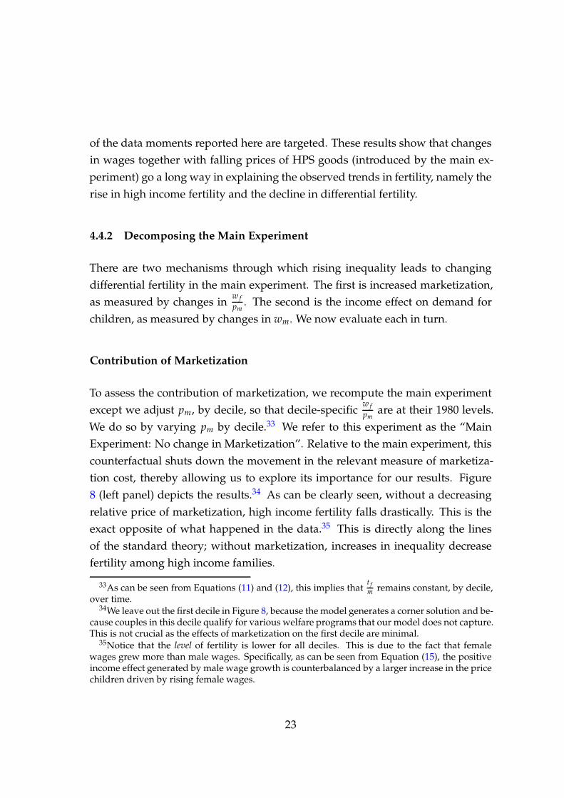
of the data moments reported here are targeted. These results show that changes
in wages together with falling prices of HPS goods (introduced by the main ex-
periment) go a long way in explaining the observed trends in fertility, namely the
rise in high income fertility and the decline in differential fertility.
4.4.2 Decomposing the Main Experiment
There are two mechanisms through which rising inequality leads to changing
differential fertility in the main experiment. The first is increased marketization,
as measured by changes inw f
pm. The second is the income effect on demand for
children, as measured by changes in wm. We now evaluate each in turn.
Contribution of Marketization
To assess the contribution of marketization, we recompute the main experiment
except we adjust pm, by decile, so that decile-specificw f
pmare at their 1980 levels.
We do so by varying pm by decile.33 We refer to this experiment as the “Main
Experiment: No change in Marketization”. Relative to the main experiment, this
counterfactual shuts down the movement in the relevant measure of marketiza-
tion cost, thereby allowing us to explore its importance for our results. Figure
8 (left panel) depicts the results.34 As can be clearly seen, without a decreasing
relative price of marketization, high income fertility falls drastically. This is the
exact opposite of what happened in the data.35 This is directly along the lines
of the standard theory; without marketization, increases in inequality decrease
fertility among high income families.
33As can be seen from Equations (11) and (12), this implies thatt f
m remains constant, by decile,over time.
34We leave out the first decile in Figure 8, because the model generates a corner solution and be-cause couples in this decile qualify for various welfare programs that our model does not capture.This is not crucial as the effects of marketization on the first decile are minimal.
35Notice that the level of fertility is lower for all deciles. This is due to the fact that femalewages grew more than male wages. Specifically, as can be seen from Equation (15), the positiveincome effect generated by male wage growth is counterbalanced by a larger increase in the pricechildren driven by rising female wages.
23

Column 3 of Table 2 reports the results for this counterfactual experiment. We
see that, without the fall in the price of marketization, high income fertility coun-
terfactually falls by 27%. More importantly, and consistent with the standard
model, MDF counterfactually falls, using both measures. This in turn decreases
college attainment by 0.53 p.p. as opposed to the 1.70 p.p. increase the data mea-
sures. This is despite the fact that rising male inequality is at work here. Thus,
as we observe above, a naïve modeler, working in 1980 and ignoring marketiza-
tion, would have predicted a widening of differential fertility and thus a decline
in college attainment rates over time if she had been given perfect foresight over
actual income distributions.36 Adding this counterfactual decrease implied by
the standard theory to the increase seen in the data, we find that the bias from
ignoring changes in marketization is 2.2 percentage points of college attainment.
This estimate implies that differential fertility’s impact on education is substan-
tial. To put things in perspective, 2.2 percentage points is equivalent to roughly
one-quarter of the rise in college attainment between the 1950 and 1980 cohorts
of white, non-Hispanic non-immigrant Americans (27% and 37.9%, respectively).
Thus, the bias induced by ignoring marketization is both quantitatively large and
changes the sign of the estimated implications of inequality on differential fertil-
ity, and thus education.
Contribution of Male Income Growth
To assess the contribution of changing male wages, we recompute the main ex-
periment holding the decile-specific male incomes (wm) at their 1980 levels. We
refer to this experiment as the “Main Experiment: No change in wm.” Figure 8
(right panel) illustrates our findings. As can be seen, the prediction for 2010 is
quite similar to that of the main experiment, with somewhat lower fertility rates
for high income households. The intuition is clear; those households saw a great
rise in male income which, through the income effect, should increase fertility.
36Notice that the standard theory does not allow for any marketization, while in our counter-factual exercise we do not allow the relevant cost of marketization to fall over time. Thus, whilethe two exercises are not perfectly comparable, the underlying economics is similar.
24

Shutting down this mechanism leads to less fertility.37
Column 4 of Table 2 summarizes the results for this counterfactual experiment.
When abstracting from changes in male income, high income fertility still rises
30%, which is 69% of the 43.5% increase in the main experiment. This means
that the income effect can explain at most 31% of the increase in high income
fertility. MDF1 (MDF2) increases 24% (15.1%), which is 59% (62%) of the 41%
(24.4%) increase in the main experiment, implying that the male income effect
can explain at most 41% (38%) of increased MDF. Finally, the college attainment
rates of the next generation rise by 1.60 p.p., which is 67% of the increase in the
main experiment, implying that the male income effect can explain at most 33%
of the increase in college attainment attributed to changing differential fertility.38
We note two more interesting facts about this exercise. The first is that the find-
ings are under the extreme assumption of traditional gender roles. If men bore a
time cost of children as well, then marketization would presumably be an even
stronger force for differential fertility in the model. Thus, our findings are conser-
vative. Second, we note that this measure of the impact of the income effect on
differential fertility captures all of the empirical mechanisms causing an increase
in male wages by decile, including sorting. To see this point, imagine that sort-
ing increases, with no other change in inequality. Then the higher deciles would
begin to measure higher male wages. Thus, this exercise can be thought of as
capturing the upper bound of the effect of rising marital sorting on differential
fertility.
A Further Look into the Marketization Mechanism
Delving deeper into our results, we perform two more exercises in order to disen-
tangle the roles of falling pm and rising female wage inequality on fertility. First,
37The opposite happens for the low end of the distribution where male real incomes actuallyfell over time.
38Notice that these two exercises show that marketization and the income effect do not addup to the total effect. This is because there is an interaction between the two mechanisms; whenpm decreases, the positive effect of w f on the price of children (pn) weakens, as seen in Equation(6) of the Online Appendix, thereby allowing the income effect of wages on fertility to grow instrength.
25
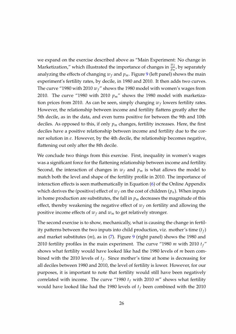
we expand on the exercise described above as “Main Experiment: No change in
Marketization,” which illustrated the importance of changes inw f
pm, by separately
analyzing the effects of changing w f and pm. Figure 9 (left panel) shows the main
experiment’s fertility rates, by decile, in 1980 and 2010. It then adds two curves.
The curve “1980 with 2010 w f ” shows the 1980 model with women’s wages from
2010. The curve “1980 with 2010 pm” shows the 1980 model with marketiza-
tion prices from 2010. As can be seen, simply changing w f lowers fertility rates.
However, the relationship between income and fertility flattens greatly after the
5th decile, as in the data, and even turns positive for between the 9th and 10th
deciles. As opposed to this, if only pm changes, fertility increases. Here, the first
deciles have a positive relationship between income and fertility due to the cor-
ner solution in e. However, by the 4th decile, the relationship becomes negative,
flattening out only after the 8th decile.
We conclude two things from this exercise. First, inequality in women’s wages
was a significant force for the flattening relationship between income and fertility.
Second, the interaction of changes in w f and pm is what allows the model to
match both the level and shape of the fertility profile in 2010. The importance of
interaction effects is seen mathematically in Equation (6) of the Online Appendix
which derives the (positive) effect of w f on the cost of children (pn). When inputs
in home production are substitutes, the fall in pm decreases the magnitude of this
effect, thereby weakening the negative effect of w f on fertility and allowing the
positive income effects of w f and wm to get relatively stronger.
The second exercise is to show, mechanically, what is causing the change in fertil-
ity patterns between the two inputs into child production, viz. mother’s time (t f )
and market substitutes (m), as in (7). Figure 9 (right panel) shows the 1980 and
2010 fertility profiles in the main experiment. The curve “1980 m with 2010 t f ”
shows what fertility would have looked like had the 1980 levels of m been com-
bined with the 2010 levels of t f . Since mother’s time at home is decreasing for
all deciles between 1980 and 2010, the level of fertility is lower. However, for our
purposes, it is important to note that fertility would still have been negatively
correlated with income. The curve “1980 t f with 2010 m” shows what fertility
would have looked like had the 1980 levels of t f been combined with the 2010
26

levels of m. Since all deciles purchase more market substitutes in 2010, fertility
is higher. However, it is clear that it is the differential rise in the use of home
production substitutes that led to a flat, or even increasing, relationship between
income and fertility.
5 The Minimum Wage, Revisited
In this section, we first discuss the theory as to why the price of marketization
(pm) has a greater effect on higher income couples. We then show empirically,
using cross state variation, that the minimum wage has a large effect on wages
in the home production substitutes sector. Our theory then implies that changes
in the minimum wage will have an impact on fertility and labor supply of high
income couples. We use the benchmark model to quantify these effects. We end
by turning to a reduced form empirical analysis to estimate the effect of the min-
imum wage on the labor supply of high income women and find even larger
effects than those implied by the model.
5.1 Minimum Wage: Theory
The effects of minimum wage laws have been widely studied, but these stud-
ies focus on the labor supply of low wage workers (Manning 2016). The theory
presented thus far makes a stark prediction; anything that changes the price of
home production substitutes, such as caretakers for children, should affect the la-
bor supply and fertility of all households. Thus, the minimum wage should also
affect the labor supply of women whose own wages are not directly impacted by
the minimum wage. We focus our attention only on women from the 5th decile
onwards in order to completely abstract from the direct effect of minimum wage
laws on wage offers. We show that the labor supply of these women is affected
through the indirect impact of minimum wage laws on the price of market sub-
stitutes for home production, as represented by pm in the model.
27
Claim 3 If ρ P p0, 1q, an increase in the minimum wage decreases labor supply, when
fertility cannot adjust, that is,Bt f
Bpm|n“n0 ą 0. Moreover the effect is differential across
the income distribution. A sufficient condition for the effect to be increasing with wages
is ρ ą 12 . That is,
B2t f
BpmBw f|n“n0 ą 0 if ρ ą 1
2 .
Proof. Follows directly from differentiating (11) with respect to pm, and then
again with respect to w f , holding n constant.
One can think of the effect of the minimum wage on labor supply holding fer-
tility constant as a short run effect. That is, if fertility decisions have already
been completed, then labor supply changes as described by Claim 3. However,
the minimum wage will also affect fertility for families that can still adjust their
fertility choices.
Claim 4 Increases in the minimum wage decrease fertility. That is, BnBpm
ă 0.
Proof. Follows directly from differentiating (15) with respect to pm.
The magnitude of the effects of the minimum wage on fertility are differential
across the income distribution, but it is theoretically ambiguous whether the mag-
nitude increases or decreases with income. We show below that, in our calibra-
tion, the richer households see the greatest decline in fertility. Notice that an
increase in the minimum wage increases the mother’s time allocated per child,
but decreases overall fertility. Therefore, the net effect on labor supply is theo-
retically ambiguous. Again, we show that in our calibration, an increase in the
minimum wage lowers female labor supply, and more so for high wage women.
5.2 Minimum Wage: Quantitative Analysis
What are the effects of minimum wage changes on marketization? To answer
this question, we first estimate the passthrough rate of the minimum wage to
HPS sector wages by exploiting cross-state variation in the minimum wage over
time. We show that the minimum wage has a strong impact on average wages
of workers producing home production substitutes. We then use our estimates
28

to conduct a policy experiment in the model by calculating a change in the price
of these goods following an increase of the federal minimum wage to $15/hour,
as suggested by Bernie Sanders during the 2016 presidential election. We ask
the model how a change in pm in line with this minimum wage increase would
affect labor supply and fertility across the income distribution. We end with a fur-
ther comparison of the model-implied labor elasticity with our own IV estimates
based on US cross-state data.
Using CPS data from 1980-2010, we compute the real wage of workers in the in-
dustries of the economy associated with home production substitutes.39 Figure
10 shows the distribution of the real wage, relative to the minimum wage, both
for the industries of the economy associated with home production substitutes
and other sectors of the economy. The figure clearly shows that workers in in-
dustries of the economy associated with home production substitutes are much
more likely to earn wages that are close to the minimum wage.
In order to infer the effect of the minimum wage on the wages of home produc-
tion substitute sector workers, we estimate regressions of the following structure:
wHPSist “ α ` βwmin
st ` γwst ` δbelow ` δt ` δs ` δage ` δeduc ` δHispan ` δrace ` δocc ` ǫist,
(21)
where wHPSist is the real wage of individual i working in the HPS sector, in state s
in year t, wminst is the real minimum wage in state s in year t. This is computed
as the maximum between the state and the federal minimum wage.40 wst is the
average wage of workers outside of the HPS sector in year t and state s. This
allows us to control for state level economic fluctuations that may affect wages
in the HPS sector.41 δt, δs, δage, δeduc, δHispan, δrace, and δocc are year dummies, state
dummies, and demographic controls including age dummies, educational dum-
mies, a dummy for being Hispanic, race dummies, and occupational dummies,
respectively. δbelow is an indicator that is equal to one if that person is making at
least the minimum wage and zero otherwise. We include this variable to control
39The selection of these industries follows Mazzolari & Ragusa (2013).40The data source for the minimum wage by state and year is Vaghul & Zipperer (2016).41Our results below show that this variable is not important quantitatively or statistically for
our findings.
29

for the fact that there are many workers, roughly 30%, for whom the minimum
wage does not seem to be binding. While we are not proposing a theory as to
why these workers are paid less, we want to include them separately in our re-
gression.42 ǫist is an error term.
Estimating (21) using OLS may yield an upward biased estimate of β if states
tend to raise the minimum wage during good economic conditions, when wages
in general are rising. We take two approaches to address this issue. First, we es-
timate (21) including on the right hand side the average wage in state s and year
t.43 The idea is that if HPS sector workers’ wages have similar cyclicality as the
rest of the workers in the economy, then the estimate of the relative wage implic-
itly controls for economic conditions. Second, we take an instrumental variables
approach along the lines of Baskaya & Rubinstein (2012). The approach relies on
two assumptions. The first is that the federal minimum wage is exogenous to
local economic conditions, and therefore exempt from the critique above. How-
ever, whether or not the federal minimum wage binds is endogenous to the state.
Accordingly, the second assumption is that the level of liberalism in the state de-
termines how likely the federal minimum wage is to bind. Thus, our instrument
for the minimum wage in state s and year t is the interaction between the federal
minimum wage in year t and an index of state s liberalism from before the sample
time period (Berry, Ringquist, Fording & Hanson 1998, Berry, Fording, Ringquist,
Hanson & Klarner 2010).44
The coefficient of interest is β, which shows the dollar change in HPS sector
wages when the minimum wage increases by a dollar. Table 3 reports the re-
sults of the estimation. Column 1 controls for year and state fixed effects and for
having a wage that is below or above the minimum wage. Column 2 adds the
state average of real wages. Column 3 repeats Column 1 but replaces year fixed
effects with region-year fixed effects. Column 4 adds to Column 3 demographic
42For example, about 9 percent of workers in this sector are in managerial occupations, ofwhom 90 percent earn wages above the minimum wage with an average of 2.5 times the mini-mum wage.
43We calculate this average wage without workers in the home production substitute sector inorder to avoid the reflection problem (Manski 1993).
44We use the average of their nominate measure of state government ideology from 1960–1980.The index of state liberalism has a range of 1 to 100, with more liberal states receiving a higherscore, with an average (standard deviation) of 62.3 (11.3).
30

controls. Column 5 adds to Column 4 the state real wage. As can be seen by com-
paring these columns, the estimate of the impact of the minimum wage on the
wages in the HPS sector is relatively stable, declining slightly only when adding
the demographic controls. The OLS estimates thus imply that a $1 increase in the
minimum wage yields approximately a 65-77 cent increase in wages in the HPS
sector. Columns 6–10 repeat Columns 1–5, but instruments for the effective min-
imum wage in the state using the interaction of state liberalism and the federal
minimum wage as described above. The IV estimates indicate that a $1 increase
in the minimum wage yields approximately a 55-75 cent increase in HPS wages.45
To calculate how a change in the minimum wage to $15/hour affects the aver-
age wage in the HPS sector in 2010, we proceed as follows. First, we calculate
the average wage in the HPS sector. Then, we create a counterfactual wage for
everyone. This wage is equal to the actual wage if the person earned less than
the minimum wage. That is, we assume that people who earn less than the mini-
mum wage are unaffected by changes in the minimum wage.46 For everyone else,
their counterfactual wage is equal to their old wage + (15-minimum wage)*0.58.
That is, we increase their wages by the estimated β from Column 10, our most
demanding specification in Table 3, multiplied by $15 less the minimum wage
in that individual’s state in 2010. We then compare the average of this counter-
factual wage to the average observed wage, and find it to be 21.1 percent higher.
Using the price of m, as given by (17), along with the inferred parameter values
described in Section 4, we find that a 21.1% increase in HPS wages would imply
a 12.8% increase in pm. Thus, for our exercise, we increase pm by 12.8%. We fo-
cus on couples in the top half of the income distribution whose own wages are
presumably unaffected by changes in the minimum wage.
45We also estimated (21) in log-log specifications which follow Table 3. In all specificationswe obtain estimates that are highly significant and approximately equal to 0.5, with no cleardifference between the OLS and the 2SLS estimates. An elasticity of 0.5 would imply a somewhatlarger effect of changing the minimum wage on pm than the one implied by the level regressionsreported in Table 3.
46 We are unsure why a person in our sample is earning less than minimum wage. It couldbe that this is a result of misreported data, lack of enforcement of the minimum wage, or anuncovered sector (waiters). To be conservative, we assume these people are unaffected by theminimum wage. Had we assumed them to be affected, then the counterfactual wage estimatedhere would be even higher, yielding a greater estimated impact of the minimum wage on homeproduction substitute sector wages.
31

The results are shown in Figure 11. The top panel shows fertility under the higher
minimum wage relative to the benchmark model fertility in 2010. The bottom
panel shows the relative mother’s time at home. A higher minimum wage de-
creases fertility, and more so for higher income households. It also increases
mother’s time at home, and more so for higher income households. The magni-
tudes are large. A 10th (5th) decile household decreases fertility by 12.1% (8.8%),
while the mother spends 9.0% (2.4%) more time at home. Notice that these num-
bers are for women under the assumption that they can adjust fertility. What
about those who are “locked in” their fertility choice? We recalculate changes in
mother’s time at home keeping the model’s fertility fixed. A 10th decile mother
increases time at home by 24.0%, while a 5th decile mother increases it by 12.3%.
These numbers are larger as the family has not had a chance to scale back fertility.
The short run effect on labor supply is also significant. The average reduction in
labor supply by women in the 9th and 10th deciles is 3.25%. We find the elastic-
ity of high income female labor supply with respect to the minimum wage to be
roughly ´0.1 in the model.
In order to verify this model prediction, we estimate directly from the data the
effect of the minimum wage on the labor supply of high income women. Specifi-
cally, we estimate regressions of the following structure:
log Hoursist “ α ` β log wminst ` δt ` δs ` δage ` δeduc ` δInd ` δocc ` ǫist, (22)
where log Hoursist is the log of yearly hours supplied by woman i, living in state
s, in year t. All other variables have already been described. Notice that β is
the elasticity of labor supply with respect to the minimum wage. We use CPS
data for the years 1980–2010. Our sample is comprised of white non-Hispanic
married women aged 25 to 54, whose real hourly wage is in the 9th or 10th decile
in each five year age group, state, and year.47 Again, as in the estimation of β in
Equation (21), estimating (22) with OLS might induce an upward bias if hours of
high income women and the state minimum wage are procyclical. To overcome
47 We drop 1% of outlying observations, specifically those groups with top wages of less than10.9 dollars per hour or more than 60 dollars per hour, measured in 1999 dollars.
32
this issue we estimate (22) using 2SLS when, again, state s minimum wage in
year t is instrumented with the interaction between the federal minimum wage
in year t and an index of state s liberalism from before the sample period.
Table 4 reports estimates of β. Column 1 only controls for year and state fixed ef-
fects. Column 2 repeats column 1 but replaces year fixed effects with region-year
fixed effects. Column 3 adds to Column 2 age and education fixed effects. Col-
umn 4 adds to Column 3 industry fixed effects, Column 5 replaces the industry
fixed effects in Column 4 with occupation fixed effects. Finally, Column 6 in-
cludes both industry and occupation fixed effects. As can be seen from the table,
all of the OLS estimates are very close to 0 and none are even remotely signifi-
cant. Columns 7–12 repeat Columns 1–6, but instrument for the state minimum
wage. All of the estimates are statistically significant and economically meaning-
ful. They imply that the elasticity of labor supply of high income women with
respect to the minimum wage is in the range of ´0.66 to ´0.41. This empirical
elasticity is thus larger than that of the model.
Finally, Table 5 repeats Table 4 for men. As can be seen from the table, all the OLS
and the 2SLS estimates are close to 0 and none are even remotely significant. This
is exactly what is expected under the assumption of traditional gender roles.
6 Sorting
In this section we discuss how marketization affects the endogenous incentives
for marital sorting by education. Greenwood et al. (2016) show how a narrowing
gender wage gap, rising skill premium, and technological improvement in home
goods (cheaper marketization) lead to, among other things, a rise in sorting. The
intuition is as follows. When the gender gap is narrow, women’s wages are rela-
tively more important for the household, increasing the desire for men to marry
higher wage women. The same is true as the skill premium rises. More rele-
vant for our story, they find that cheaper marketization leads to a rise in married
women’s labor force participation, which they argue is important for the desire
to sort. “A skilled man is indifferent on economic grounds between a skilled
33

and unskilled woman if neither of them works, assuming that skill doesn’t affect
a woman’s production value at home. When both work, however, the skilled
woman becomes the more attractive partner, at least from an economic point of
view” (Greenwood et al. 2016, p. 35). Fertility is not discussed in Greenwood
et al. (2016). However, if children comprise an additional benefit to marriage, the
mechanism proposed in this paper would reinforce the mechanisms they study.
To see this point, consider a man who is choosing between two women, one with
a high wage and the other with a low wage. In 1980, the man would face a trade-
off. The high wage woman would provide more income, and thus consumption,
but at a cost of fewer children. In 2010, the high wage women could marketize her
time with children, such that there is no more tradeoff. That is, the man would
not have to choose between high wages and a large family, yielding more of an
incentive to marry a high wage woman. This argument is consistent with the
fact that marriage outcomes for college educated women have improved relative
to non college educated women, measured by the fraction of those ever married
or currently married (Figure 12, for data on white non-Hispanic women, ages
35–44).
While these data are not conclusive, they are suggestive of a path for promising
future research.
7 Conclusions
In this paper we have shown that the relationship between income and fertility
has flattened between 1980 and 2010 in the US, a time of increasing inequality,
as the rich increased their fertility. These facts challenge the standard theory ac-
cording to which rising inequality should steepen this relationship. We propose
that marketization of parental time costs can explain the changing relationship
between income and fertility. We show this result both theoretically and quanti-
tatively, after disciplining the model on US data. When abstracting from changes
in marketization, the model behaves according to standard theory, generating a
drop in differential fertility contrary to what happened in the data. We discuss
implications for college attainment.
34

We have used the calibrated model to shed new light on the effects of changes
in the minimum wage. Specifically, we have shown that an increase in the min-
imum wage to $15/hour, as per Bernie Sanders, would imply an increase in the
cost of market good substitutes for home production of about 13 percent. This
increase would have a significant detrimental effect on the labor supply and fertil-
ity of women, whose own wages are not directly affected by the minimum wage
increase. The response is higher for high wage women.
We ended with a discussion on the insights our theory offers for the literature of
the economics of marital sorting.
35
References
Aguiar, M. & Hurst, E. (2007), ‘Life-cycle prices and production’, The American
Economic Review 97(5), 1533–1559.
Akbulut, R. (2011), ‘Sectoral changes and the increase in women’s labor force
participation’, Macroeconomic Dynamics 15(2), 240–264.
Attanasio, O., Hurst, E. & Pistaferri, L. (2012), The evolution of income, consump-
tion, and leisure inequality in the us, 1980-2010. NBER WP 17982.
Attanasio, O., Low, H. & Sanchez-Marcos, V. (2008), ‘Explaining changes in fe-
male labour supply in a life-cycle model’, The American Economic Review
98(4), 1517–1552.
Autor, D. H., Katz, L. F. & Kearney, M. S. (2008), ‘Trends in u.s. wage inequality:
Revising the revisionists’, Review of Economics and Statistics 90, 300–323.
Bar, M. & Leukhina, O. (2009), ‘To work or not to work: Did tax reforms affect
labor force participation of married couples?’, The B.E. Journal of Macroeco-
nomics (Contributions) 9(1), 1–28.
Baskaya, Y. S. & Rubinstein, Y. (2012), Using federal minimum wages to identify
the impact of minimum wages on employment and earnings across the u.s.
states. Unpublished Manuscript.
Becker, G. S. & Lewis, G. H. (1973), ‘On the interaction between the quantity and
quality of chldren’, Journal of Political Economy 81, S279–S288.
Becker, G. S. & Tomes, N. (1976), ‘Child endowments and the quantity and quality
of children’, Journal of Political Economy 84, S143–S162.
Berry, W. D., Fording, R. C., Ringquist, E. J., Hanson, R. L. & Klarner, C. (2010),
‘Measuring citizen and government ideology in the american states: A re-
appraisal’, State Politics and Policy Quarterly 10, 117–135.
Berry, W. D., Ringquist, E. J., Fording, R. C. & Hanson, R. L. (1998), ‘Measuring
citizen and government ideology in the american states, 1960-93’, American
Journal of Political Science 42, 327–348.
36
Buera, F. J., Kaboski, J. P. & Zhao, M. Q. (2017), ‘The rise of services: the role of
skills, scale, and female labor supply’, Journal of Human Capital . forthcom-
ing.
Cerina, F., Moro, A. & Rendall, M. (2018), The role of gender in employment
polarization. Unpublished Manuscript.
Cortés, P. & Pan, J. (2013), ‘Household production: Foreign domestic workers and
native labor supply in hong kong’, Journal of Labor Economics 31(2), 327–371.
Cortés, P. & Pan, J. (Forthcoming), ‘When time binds: Substitutes to household
production, returns to working long hours and the gender wage gap among
the highly skilled’, Journal of Labor Economics .
Cortés, P. & Tessada, J. (2011), ‘Low-skilled immigration and the labor supply
of highly skilled women’, American Economic Journal: Applied Economics
3(1), 88–123.
de la Croix, D. & Doepke, M. (2003), ‘Inequality and growth: Why differential
fertility matters’, The American Economic Review 93(4), 1091–1113.
de la Croix, D. & Doepke, M. (2004), ‘Public versus private education when dif-
ferential fertility matters’, Journal of Development Economics 73, 607–629.
Doepke, M. (2004), ‘Accounting for fertility decline during the transition to
growth’, Journal of Economic Growth 9(3), 347–383.
Doepke, M. & Kindermann, F. (2016), Bargaining over babies: Theory, evidence,
and policy implications. NBER Working Paper w22072.
Duernecker, G. & Herrendorf, B. (2018), ‘On the allocation of time - a quantitative
analysis of the roles of taxes and productivities’, European Economic Review
102, 169–187.
Furtado, D. (2016), ‘Fertility responses of high-skilled native women to immi-
grant inflows’, Demography 53, 27–53.
Galor, O. & Moav, O. (2002), ‘Natural selection and the origin of economic
growth’, Quarterly Journal of Economics 117(4), 1113–1191.
Galor, O. & Weil, D. N. (1996), ‘The gender gap, fertility, and growth’, The Ameri-
can Economic Review 86(3), 374–387.
37

Galor, O. & Weil, D. N. (2000), ‘Population, technology, and growth: From
malthusian stagnation to the demographic transition and beyond’, The Amer-
ican Economic Review 90(4), 806–828.
Gobbi, P. (2018), ‘Childcare and commitment within households’, Journal of Eco-
nomic Theory 176, 503–551.
Greenwood, J., Guner, N., Kocharkov, G. & Santos, C. (2016), ‘Technology and
the changing family’, American Economic Journal: Macroeconomics 8(1), 1–41.
Greenwood, J., Guner, N. & Vandenbroucke, G. (2017), ‘Family economics writ
large’, Journal of Economic Literature . forthcoming.
Greenwood, J., Seshadri, A. & Vandenbroucke, G. (2005), ‘The baby boom and
baby bust’, The American Economic Review 95(1), 183–207.
Greenwood, J., Seshadri, A. & Yorukoglu, M. (2005), ‘Engines of liberation’, Re-
view of Economic Studies 72(1), 109–133.
Guner, N., Kaygusuz, R. & Ventura, G. (2012), ‘Taxation and household labour
supply’, The Review of Economic Studies 79, 1113–1149.
Hazan, M. & Zoabi, H. (2015), ‘Do highly educated women choose smaller fami-
lies?’, The Economic Journal 125(587), 1191–1226.
Heathcote, J., Perri, F. & Violante, G. (2010), ‘Unequal we stand: An empirical
analysis of economic inequality in the united states 1967-2006’, Review of
Economic Dynamics 13(1), 15–50.
Jones, L. E., Schoonbroodt, A. & Tertilt, M. (2010), Fertility theories: Can they ex-
plain the negative fertility-income relationship?, in J. Shoven, ed., ‘Demog-
raphy and the Economy’, University of Chicago Press, pp. 43–100.
Jones, L. E. & Tertilt, M. (2008), An economic history of fertility in the u.s.: 1826-
1960, in P. Rupert, ed., ‘Frontiers of Family Economics’, Emerald, pp. 165 –
230.
Kaygusuz, R. (2010), ‘Taxes and female labor supply’, Review of Economic Dynam-
ics 13, 725–741.
Lino, M., Kuczynski, K., Rodriguez, N. & Schap, T. (2017), Expenditures on chil-
dren by families, 2015, Technical report, United States Department of Agri-
culture.
38

Manning, A. (2016), The elusive employment of the minimum wage. CEP Dis-
cussion Paper No 1428.
Manski, C. F. (1993), ‘Identification of endogenous social effects: The reflection
problem’, The Review of Economic Studies 60(3), 531–542.
Mazzolari, F. & Ragusa, G. (2013), ‘Spillovers from high-skill consumption to
low-skill labor markets’, The Review of Economics and Statistics 95(1), 74–86.
Moav, O. (2005), ‘Cheap children and the persistence of poverty’, The Economic
Journal 115(500), 88–110.
Rendall, M. (2018), ‘Female market work, tax regimes, and the rise of the service
sector’, Review of Economic Dynamics 28, 269–289.
Ruggles, S. J., Alexander, T., Genadek, K., Goeken, R., Schroeder, M. B. & Sobek,
M. (2010), Integrated Public Use Microdata Series: Version 5.0 [Machine-readable
database], Minneapolis, MN.
Sato, K. (1967), ‘A two-level constant elasticity of substitution production func-
tion’, The Review of Economic Studies 34(2), 201–218.
Shang, Q. & Weinberg, B. A. (2013), ‘Opting for families: Recent trends in the
fertility of highly educated women’, Journal of Population Economics 26(1), 5–
32.
Siegel, C. (2017), ‘Female relative wages, household specialization and fertility’,
Review of Economic Dynamics 24, 152–174.
Vaghul, K. & Zipperer, B. (2016), Historical state and sub-state minimum wage
data. Washington Center for Equitable Growth.
Vogl, T. (2016), ‘Differential fertility, human capital, and development’, Review of
Economic Studies 83(1), 365–401.
39

Table 1: Calibrated Parameter Values
Parameter Interpretation Value Indentification
α Weight on # of children 0.45 Fertility
β Weight on quality of children 0.67 Fertility
η Basic education 2.06 Fertility
θ Exponent π 0.43 College Attainment
b Scaling 0.87 College Attainment
ρ Elasticity mother’s time/m 0.59 Labor Supply
φ Share of mother’s time 0.90 Labor Supply
A TFP child production 3.77 Index of Marketization
pm,1980 Price of market substitutes 1980 1 Normalization
pe Cost of education 1 Normalization
Table 2: Results: Model Mechanisms
Data Main Experiment
Baseline No change in No change
Marketization in wm
(1) (2) (3) (4)
%∆ High Inc Fert 40.0% 43.5% -27.6% 30.0%
%∆ MDF1 38.5% 41.0% -2.4% 24.0%
%∆ MDF2 18.6% 24.4% -4.4% 15.1%
∆ CG (pp) 1.70 2.40 -0.53 1.60
Notes: “High Inc Fert” is the number of children born to the top 2 deciles. “MDF1”is the fertility of the top two deciles relative to the fertility of the 2nd decile. “MDF2”is the fertility of the top half of the income distribution relative to the fertility ofthe bottom half of the income distribution. “CG” is the fertility-driven measure ofaggregate college attainment. See Footnotes 30 and 31 for the formal definitions ofthese variables. All changes refer to between 1980 and 2010. Column (1), “Data”,reports data changes. Column (2) , “Baseline”, reports changes implied by the MainExperiment. Column (3) “No change in Marketization” and Column (4), “No changein wm” report changes for the two counterfactual experiments that supplement theMain Experiment, as described in Section 4.4.2.
40
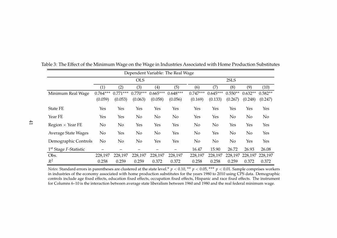
Table 3: The Effect of the Minimum Wage on the Wage in Industries Associated with Home Production Substitutes
Dependent Variable: The Real Wage
OLS 2SLS
(1) (2) (3) (4) (5) (6) (7) (8) (9) (10)
Minimum Real Wage 0.764˚˚˚ 0.771˚˚˚ 0.770˚˚˚ 0.665˚˚˚ 0.648˚˚˚ 0.747˚˚˚ 0.645˚˚˚ 0.550˚˚ 0.632˚˚ 0.582˚˚
(0.059) (0.053) (0.063) (0.058) (0.056) (0.169) (0.133) (0.267) (0.248) (0.247)
State FE Yes Yes Yes Yes Yes Yes Yes Yes Yes Yes
Year FE Yes Yes No No No Yes Yes No No No
Region ˆ Year FE No No Yes Yes Yes No No Yes Yes Yes
Average State Wages No Yes No No Yes No Yes No No Yes
Demographic Controls No No No Yes Yes No No No Yes Yes
1st Stage F-Statistic – – – – – 16.47 15.90 26.72 26.93 26.08
Obs. 228,197 228,197 228,197 228,197 228,197 228,197 228,197 228,197 228,197 228,197
R2 0.258 0.259 0.259 0.372 0.372 0.258 0.258 0.259 0.372 0.372
Notes: Standard errors in parentheses are clustered at the state level.˚ p ă 0.10, ˚˚ p ă 0.05, ˚˚˚ p ă 0.01. Sample comprises workersin industries of the economy associated with home production substitutes for the years 1980 to 2010 using CPS data. Demographiccontrols include age fixed effects, education fixed effects, occupation fixed effects, Hispanic and race fixed effects. The instrumentfor Columns 6–10 is the interaction between average state liberalism between 1960 and 1980 and the real federal minimum wage.
41
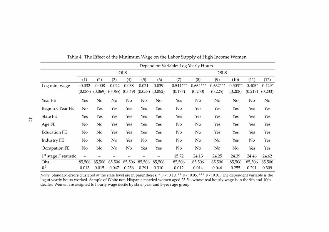
Table 4: The Effect of the Minimum Wage on the Labor Supply of High Income Women
Dependent Variable: Log Yearly Hours
OLS 2SLS
(1) (2) (3) (4) (5) (6) (7) (8) (9) (10) (11) (12)
Log min. wage -0.032 -0.008 -0.022 0.038 0.021 0.039 -0.544˚˚˚ -0.664˚˚˚ -0.632˚˚˚ -0.503˚˚ -0.405˚ -0.429˚
(0.087) (0.069) (0.065) (0.049) (0.053) (0.052) (0.177) (0.250) (0.225) (0.208) (0.217) (0.233)
Year FE Yes No No No No No Yes No No No No No
Regionˆ Year FE No Yes Yes Yes Yes Yes No Yes Yes Yes Yes Yes
State FE Yes Yes Yes Yes Yes Yes Yes Yes Yes Yes Yes Yes
Age FE No No Yes Yes Yes Yes No No Yes Yes Yes Yes
Education FE No No Yes Yes Yes Yes No No Yes Yes Yes Yes
Industry FE No No No Yes No Yes No No No Yes No Yes
Occupation FE No No No No Yes Yes No No No No Yes Yes
1st stage F statistic – – – – – – 15.72 24.13 24.25 24.39 24.46 24.62
Obs. 85,506 85,506 85,506 85,506 85,506 85,506 85,506 85,506 85,506 85,506 85,506 85,506
R2 0.013 0.015 0.047 0.256 0.291 0.310 0.012 0.014 0.046 0.255 0.291 0.309
Notes: Standard errors clustered at the state level are in parentheses. ˚ p ă 0.10, ˚˚ p ă 0.05, ˚˚˚ p ă 0.01. The dependent variable is thelog of yearly hours worked. Sample of White non-Hispanic married women aged 25-54, whose real hourly wage is in the 9th and 10thdeciles. Women are assigned to hourly wage decile by state, year and 5-year age group.
42

Table 5: The Effect of the Minimum Wage on the Labor Supply of High Income Men
Dependent Variable: Log Yearly Hours
OLS 2SLS
(1) (2) (3) (4) (5) (6) (7) (8) (9) (10) (11) (12)
Log min. wage 0.043 0.011 0.004 0.002 -0.009 -0.011 -0.118 -0.117 -0.036 0.031 -0.061 -0.032
(0.034) (0.031) (0.028) (0.026) (0.027) (0.027) (0.115) (0.149) (0.123) (0.122) (0.122) (0.119)
Year FE Yes No No No No No Yes No No No No No
Regionˆ Year FE No Yes Yes Yes Yes Yes No Yes Yes Yes Yes Yes
State FE Yes Yes Yes Yes Yes Yes Yes Yes Yes Yes Yes Yes
Age FE No No Yes Yes Yes Yes No No Yes Yes Yes Yes
Education FE No No Yes Yes Yes Yes No No Yes Yes Yes Yes
Industry FE No No No Yes No Yes No No No Yes No Yes
Occupation FE No No No No Yes Yes No No No No Yes Yes
1st stage F statistic – – – – – – 15.27 25.10 25.18 25.42 25.32 25.63
Obs. 100,243 100,243 100,243 100,243 100,243 100,243 100,243 100,243 100,243 100,243 100,243 100,243
R2 0.013 0.015 0.067 0.160 0.202 0.211 0.013 0.015 0.067 0.160 0.202 0.211
Notes: Standard errors clustered at the state level are in parentheses. ˚ p ă 0.10, ˚˚ p ă 0.05, ˚˚˚ p ă 0.01. The dependent variable is thelog of yearly hours worked. Sample of White non-Hispanic married men aged 25-54, whose real hourly wage is in the 9th and 10thdeciles. Men are assigned to hourly wage decile by state, year and 5-year age group.
43

1.87
1.54
1.39 1.19
2.36
2.01
1.85
1.53
1.70
1.00
1.50
2.00
2.50
<12 12 13-15 16 >16
Fertility
Education
1980 2010
Figure 1: Fertility by Women’s Education 1980 & 2010.Notes: Authors calculations using Census and American Community Survey Data, using all native-born American women.Fertility rates are hybrid fertility rates. “ă 12” refers to women with less than a high school degree. “12” refers to womenwho graduated high school. “13-15” refers to women with some college. “16” refers to college graduates. “ą 16” refers towomen with advanced degrees.
44

2.96 2.942.77
2.55 2.50
2.312.23
2.12
1.941.82
3.38
2.972.82
2.67 2.662.50 2.55
2.752.60 2.66
1.00
1.50
2.00
2.50
3.00
3.50
4.00
1 2 3 4 5 6 7 8 9 10
Fer
tili
ty
Income Decile
1980 2010
Figure 2: Fertility by Income Decile 1980 & 2010.Notes: Authors calculations using Census and American Community Survey Data. The sample is restricted to white, non-Hispanic married women. Fertility rates are hybrid fertility rates, constructed by age-specific deciles. Deciles are constructedusing total household income.
45
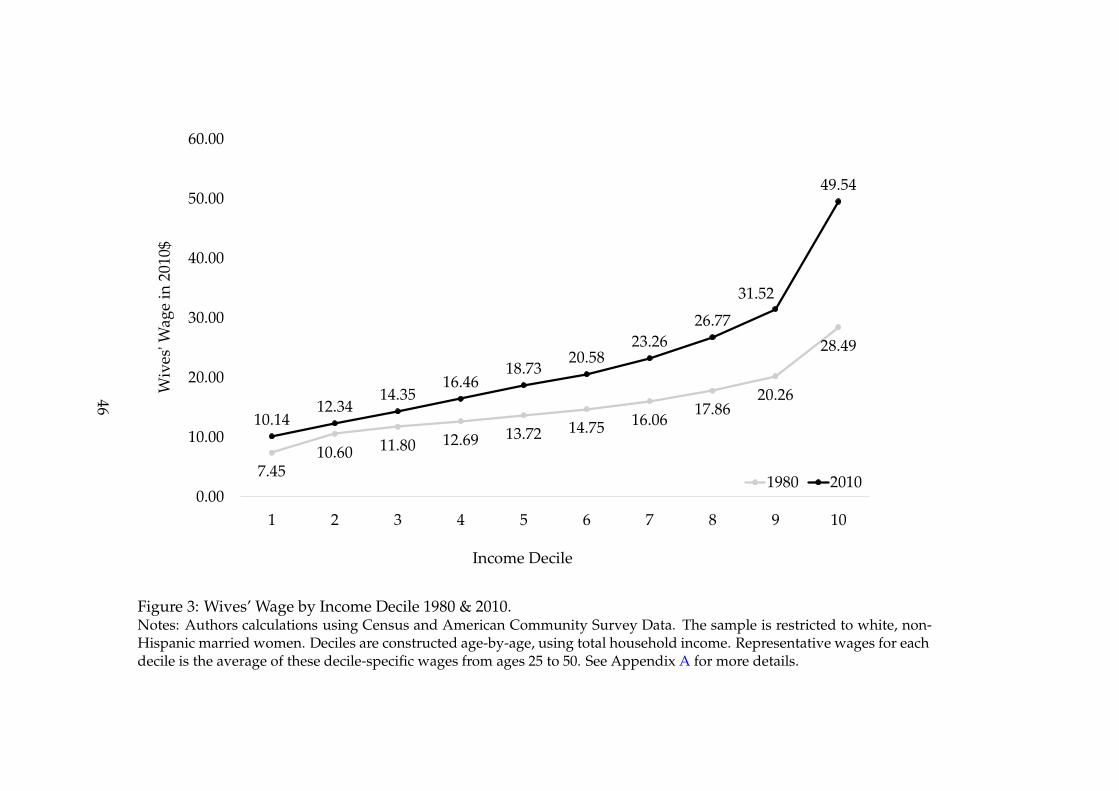
7.4510.60 11.80 12.69 13.72 14.75 16.06
17.8620.26
28.49
10.1412.34
14.3516.46
18.7320.58
23.26
26.77
31.52
49.54
0.00
10.00
20.00
30.00
40.00
50.00
60.00
1 2 3 4 5 6 7 8 9 10
Wiv
es' W
age
in 2
010$
Income Decile
1980 2010
Figure 3: Wives’ Wage by Income Decile 1980 & 2010.Notes: Authors calculations using Census and American Community Survey Data. The sample is restricted to white, non-Hispanic married women. Deciles are constructed age-by-age, using total household income. Representative wages for eachdecile is the average of these decile-specific wages from ages 25 to 50. See Appendix A for more details.
46

12.47
17.9621.30
23.6426.02
28.1530.69
33.58
38.43
51.17
12.49
17.0619.95
22.6225.09
28.3631.50
36.34
43.87
63.89
0.00
10.00
20.00
30.00
40.00
50.00
60.00
70.00
1 2 3 4 5 6 7 8 9 10
Hu
sban
ds'
Wag
e in
201
0$
Income Decile
1980 2010
Figure 4: Husbands’ Wage by Income Decile 1980 & 2010.Notes: Authors calculations using Census and American Community Survey Data. The sample is restricted to white, non-Hispanic married men. Deciles are constructed age-by-age, using total household income. Representative wages for eachdecile is the average of these decile-specific wages from ages 25 to 50. See Appendix A for more details.
47
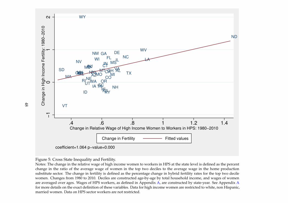
ALAK
AZAR CA
CO
CT
DE
FLGA
HIID
ILIN
IAKSKY
LA
ME
MD
MAMI
MN
MS
MOMT
NE
NV
NH
NJ
NM
NY
NC
ND
OHOK
OR
PA
RISC
SD
TN
TX
UT
VT
VA
WA
WV
WI
WY
−1
01
2C
ha
ng
e in
Hig
h I
nco
me
Fe
rtili
ty:
19
80
−2
01
0
.4 .6 .8 1 1.2 1.4Change in Relative Wage of High Income Women to Workers in HPS: 1980−2010
Change in Fertility Fitted values
coefficient=1.064 p−value=0.000
Figure 5: Cross State Inequality and Fertility.Notes: The change in the relative wage of high income women to workers in HPS at the state level is defined as the percentchange in the ratio of the average wage of women in the top two deciles to the average wage in the home productionsubstitute sector. The change in fertility is defined as the percentage change in hybrid fertility rates for the top two decilewomen. Changes from 1980 to 2010. Deciles are constructed age-by-age by total household income, and wages of womenare averaged over ages. Wages of HPS workers, as defined in Appendix A, are constructed by state-year. See Appendix Afor more details on the exact definition of these variables. Data for high income women are restricted to white, non Hispanic,married women. Data on HPS sector workers are not restricted.
48

2 4 6 8 10
Income Decile
0
0.2
0.4
0.6
0.8
1
Tim
e a
t H
om
e
2 4 6 8 10
Income Decile
1.5
2
2.5
3
3.5
Fert
ility
2 4 6 8 100
0.2
0.4
0.6
0.8
1
Education
2 4 6 8 100
5
10
15
Mark
etization I
ndex
Model, 1980 Data, 1980
Figure 6: Model FitNotes: The top left panel, “Time at Home”, is mother’s time at home as measured by women’s time not working in the data,and t f in the model. The top right panel, “Fertility”, is n in the model and hybrid fertility rates in data. “Education” is thefraction of children born to each decile who graduate college in the data and πpeq in the model. “Marketization index” is
the expenditures on babysitters, by decile, relative to the 1st decile in the data, andpmmpdqpmmp1q in the model, where mpdq is the
amount of market goods m purchased by decile d. “Model, 1980” refers to the calibrated model in 1980. “Data, 1980” refersto the relevant data described in this note and the text.
49

2 4 6 8 10
Income Decile
0
0.2
0.4
0.6
0.8
1
Tim
e a
t H
om
e
2 4 6 8 10
Income Decile
1.5
2
2.5
3
3.5
Fert
ility
2 4 6 8 100
0.2
0.4
0.6
0.8
1
Education
2 4 6 8 100
5
10
15
Mark
etization I
ndex
Data, 1980 Data, 2010 High Benchmark
Figure 7: Main Experiment.Notes: The top left panel, “Time at Home”, is mother’s time at home as measured by women’s time not working in the data,and t f in the model. The top right panel, “Fertility”, is n in the model and hybrid fertility rates in data. “Data 2010” refersto the data, as described in the text. “Benchmark”, “High ǫ” and “Low ǫ” refer to the main experiment’s prediction for 2010,for the benchmark case, the “high ǫ” case, and the “low ǫ” case, respectively. The “main experiment” refers to introducingthe 2010 values of wm, w f , and pm into the calibrated model.
50

2 4 6 8 10
Income Decile
1.2
1.4
1.6
1.8
2
2.2
2.4
2.6
2.8
3
3.2
Fert
ility
Main Experiment, 1980
Main Experiment, 2010
Main Experiment, No ch. Marketization, 2010
2 4 6 8 10
Income Decile
1.8
2
2.2
2.4
2.6
2.8
3
3.2
Fert
ility
Main Experiment, 1980
Main Experiment, 2010
Main Experiment, No ch. wm
, 2010
Figure 8: Counterfactuals.Notes: Fertility is n in the model. “Main Experiment 1980” is the model calibrated to 1980, while “Main Experiment 2010” isthe Main Experiment in both panels. Left panel: The curve labeled “Main Experiment: No ch. Marketization” is fertility in
the 2010 model using the same relative price of market substitutes (w f
pm), by decile, as in 1980. Right Panel: The curve labeled
“Main Experiment: No ch. wm” is fertility in the 2010 model using the male wages from 1980.
51
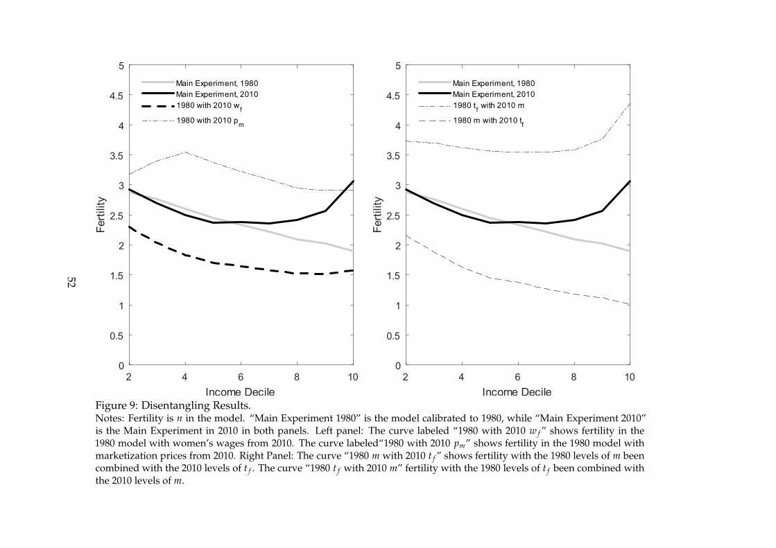
2 4 6 8 10
Income Decile
0
0.5
1
1.5
2
2.5
3
3.5
4
4.5
5
Fert
ility
Main Experiment, 1980
Main Experiment, 2010
1980 with 2010 wf
1980 with 2010 pm
2 4 6 8 10
Income Decile
0
0.5
1
1.5
2
2.5
3
3.5
4
4.5
5
Fert
ility
Main Experiment, 1980
Main Experiment, 2010
1980 tf with 2010 m
1980 m with 2010 tf
Figure 9: Disentangling Results.Notes: Fertility is n in the model. “Main Experiment 1980” is the model calibrated to 1980, while “Main Experiment 2010”is the Main Experiment in 2010 in both panels. Left panel: The curve labeled “1980 with 2010 w f ” shows fertility in the1980 model with women’s wages from 2010. The curve labeled“1980 with 2010 pm” shows fertility in the 1980 model withmarketization prices from 2010. Right Panel: The curve “1980 m with 2010 t f ” shows fertility with the 1980 levels of m beencombined with the 2010 levels of t f . The curve “1980 t f with 2010 m” fertility with the 1980 levels of t f been combined withthe 2010 levels of m.
52

0.2
.4.6
.8
1 2 3 4 5 6 7 8 9 10Relative Wage
Home Production Substitutes Others
Figure 10: Wage DistributionNotes: The distribution of real wages, relative to the effective real minimum wage in each state and year, by sector of theeconomy. Data from Current Population Survey, 1980–2010, using all workers. Home Production Substitute sector workersas defined in Appendix A.
53

Figure 11: Minimum Wage: Quantitative Results.Notes: The top panel shows fertility (n) in the 2010 version of the model, with a $15 minimum wage, divided by fertility inthe benchmark 2010 model. The bottom panel shows mother’s time at home (t f ) in the 2010 version of the model, with a$15 minimum wage, divided by mother’s time at home in the benchmark 2010 model. The curve “With Changing Fertility”reports this ratio when fertility is allowed to change with the increased minimum wage, while the curve “Fertility LockedIn” reports this ratio when households are forced to maintain the same fertility rate as in the benchmark 2010 model.
54

.91
1.1
1.2
1.3
Rela
tive C
urr
ently M
arr
ied R
ate
s
1980 1985 1990 1995 2000 2005 2010 2015Year
.94
.96
.98
11.0
21.0
4R
ela
tive E
ver
Marr
ied R
ate
s
1980 1985 1990 1995 2000 2005 2010 2015Year
Figure 12: Marriage Markets.Notes: The left panel shows the fraction of women with at least a college degree who are currently married divided by thefraction of other women who are currently married. The right panel shows the fraction of women with at least a collegedegree who have ever been married divided by fraction of other women who have ever been married. The data is from theUS census and ACS. The sample is comprised of white, non-Hispanic women ages 35–44.
55
A Data
We employ the 1980 Census and the American Community Survey (ACS) 2010
(Ruggles, Alexander, Genadek, Goeken, Schroeder & Sobek 2010) for measuring
incomes, fertility and work hours of each spouse. Additionally, we use the Na-
tional Longitudinal Study of Youth 1997 (NLSY 97) for measuring educational
attainment of children born around 1980, by family income. Finally, we employ
the Survey of Program Participation and Income for measuring childcare expen-
diture by family income. In this study, we focus on the growth of inequality
between 1980 and 2010. These years are chosen to allow us to follow the cohort
from the NLSY 97 (born around 1980) for measuring their educational attainment
by their parental income, while still studying the period of rising income inequal-
ity as defined by Autor et al. (2008).
A.1 Mapping of Model Objects to the Data
The mapping between the model and the data is not trivial. In the model, there
is one period of adult life which aims to capture the entire working-age lifecycle.
In the data, we observe choices of various couples of different age (fertility, work
hours, etc) for a period of one year. To map the model to the data, we take the
view that a model couple goes through its lifecycle by behaving according to the
average age-specific behavior of those couples in the data that it represents.
There are ten types of couples in the model, each of measure 0.1. Each type of
couple stands in for exactly 10% of the entire population of married couples of
working age. Married couples in the data are allocated into these deciles accord-
ing to their observed income. We do so based on the ranking of the couples’
observed annual income in their group, defined by the wife’s age.
From the 1980 Census and 2010 ACS data, we need to derive decile-specific em-
pirical moments for household lifetime income, male lifetime income, male and
female wages, male and female lifetime work hours, and couple’s lifetime fer-
tility, Iyearf ,i , I
yearm,i , w
yearf ,i , w
yearm,i , hours
yearf ,i , n
yeari , hours1980
m for each decile i P r1, 2, ...10s
56

and year “ 1980, 2010. We state income and hours moments in annualized terms
and report wages in hourly terms. This is done for clarity.
We restrict attention to white non-Hispanic married couples, aged 25-55, with
the husband working at least 35 hours per week and at least 40 weeks per year,
following Autor et al. (2008). We also drop the couples in the bottom and top 2%
of the male income distribution.
All data couples assigned to a particular income decile are used to derive the
average statistics for the model couple representing that decile. To compute the
decile-specific lifetime income and hours moments for men, we first average the
appropriate quantity within the decile-age cells. For each decile, we then sum
across ages.
In the model, all men work full time throughout their life cycle, which is nor-
malized to be 1. This corresponds to the average lifetime hours of full-time male
workers in 1980, hours1980m (~2,300 hours in annualized terms). We infer the data
counterpart of wyearm,i as I
yearm,i hours1980
m . Note that the 1980 average hours are used
to derive wyearm,i in each year. This method ensures that the observed variation of
total male incomes across deciles and time will be fully reflected in the purchas-
ing power of couples in the model.
Note that when we consider say a 37 year old woman in 1980 in a given decile, we
observe her work hours, which partly reflect her number of children and their age
distribution. Our goal here, however, is to derive average working hours for a
hypothetical woman that experiences her lifecycle according to the cross-sectional
profile. We need to proxy the hours each woman would work if she were to
follow the 1980s cross-sectional fertility profile, not that of her own cohort. To this
end, we regress female work hours in a given year on the actual age distribution
of her children (i.e. number of children under 2, 2-3, 4-6, 7-10, 11 to 17), income
decile and age dummies. We then predict the average adjusted female hours in
each decile and for each age using the children’s age distribution implied by the
cross-sectional fertility profile. For each decile, we sum these average adjusted
hours across age groups to obtain hoursyearf ,i and infer the data counterpart of time
57

spent in home production tyearf ,i as
1 ´ hoursyearf ,i hours1980
m .
We infer the data counterpart of w f ,i as Iyearf ,i hours
yearf ,i (about 2,050 hours in an-
nualized terms).48 We infer the empirical counterpart of ni as a decile-specific
hybrid Total Fertility Rate (TFR), as in Shang & Weinberg (2013). We first com-
pute the average age-specific-birth-rate, based on all women in decile i. We then
sum across all ages to compute decile-specific TFR. To obtain decile-specific hy-
brid TFR, we add on the average lifetime fertility among the 25 year-old women
in the appropriate decile.49
We estimate college attainment for 1980 from NLSY97. Specifically, using the 2011
wave, we observe non-black non-Hispanic individuals, born between 1980 and
1982, and assign them into income deciles according to their parental household
income in 1996. We assume that individuals with at least four years of college
are college graduates. We measure college attainment π1980i as the fraction of
children with a college degree among all children in the appropriate decile.
Finally, we use the childcare module of the Survey of Program Participation and
Income (SIPP) to estimate relative uses of market substitutes.50 Our index mea-
sures are based off of expenditures on childcare hours purchased in the market-
place. Since this is only one aspect of marketization, we use this to target the
relative use of marketization across deciles, rather than taking the absolute expen-
diture levels literally. The implicit assumption is that there is a strong correlation
between the use of childcare and other market substitutes for parents’ time. To
calculate childcare expenditures across deciles, we break households into 5-year
age groups from 25–30 until 50–55. Within each group, we divide households
48Note that if instead we were to impute wages for non-working females via a Heckman pro-cedure and then take average wages for each decile, our model would not be able to accuratelymatch both female income and female hours. Both of these quantities are critical to our analysis.
49Why not include younger women in our analysis and use the standard measure of TFR?We model time allocation between work and home production, and therefore prefer to focus oncouples that completed educational investments. Using the hybrid fertility measure then enablesus to correctly account for the number of children.
50We use the 1990 childcare module as a proxy for the 1980 index of marketization, as this isthe earliest available data. We use the 2010 module to derive the 2010 index.
58

into deciles according to their income. We then sum the childcare expenditures
for each decile over the lifecycle. The index is this measure relative to the expen-
ditures on childcare used by decile 1. As before, our sample is married, white,
non-Hispanic households.
59


