

Page 1 of 12 © Aquaveo 2015
WMS 10.0 Tutorial
Hydraulics and Floodplain Modeling – Simplified Dam Break Learn how to run a dam break simulation and delineate its floodplain
Objectives Setup a conceptual model of stream centerlines and cross sections for the simplified dam break
(SMPDBK) model. Export the conceptual model to SMPDBK and run the analysis code. Read the
results back into WMS and delineate the floodplain to determine the impact of the dam break.
Prerequisite Tutorials Introduction – Images
Introduction – Basic Feature
Objects
Editing Elevations – DEM
Basics
Editing Elevations – Using
TINs
Required Components Data
Drainage
Map
River
Time 30-60 minutes
v. 10.0
Page 2 of 12 © Aquaveo 2015
1 Contents
1 Contents ............................................................................................................................... 2 2 Introduction ......................................................................................................................... 2 3 Preparing the Model ........................................................................................................... 2
3.1 Running TOPAZ .......................................................................................................... 2 3.2 Creating Outlets and Streams ....................................................................................... 3 3.3 Creating 1D Hydraulic Coverages ............................................................................... 5 3.4 Reading in Area Properties .......................................................................................... 6 3.5 Extracting Cross Sections ............................................................................................. 7
4 Using SMPDBK ................................................................................................................... 7 4.1 Edit Parameters ............................................................................................................ 7 4.2 Running the Simulation ................................................................................................ 8
5 Post-Processing .................................................................................................................... 9 5.1 Interpolation ................................................................................................................. 9 5.2 Getting a Background Image ...................................................................................... 10 5.3 Open Background Image ............................................................................................ 10 5.4 Floodplain Delineation ............................................................................................... 10
2 Introduction
Simplified Dam Break (SMPDBK) is a model that does just what its name says—it
models dam failures using simplified methods. One alternative to using SMPDBK is to
use sophisticated dam break models such as the National Weather Service’s (NWS)
DAMBRK model. These models require extensive data, time, and computing power.
When these data or resources are not available, SMPDBK can be used to create a “quick
and dirty” solution to the flood depths downstream of a dam failure. By combining the
SMPDBK results with the floodplain delineation and display capabilities of WMS, you
can create a good picture of the aerial extents of a flood resulting from a dam break.
3 Preparing the Model
3.1 Running TOPAZ
In this section, you will load the DEM and run TOPAZ to compute the flow directions
and flow accumulations. The purpose of doing this is to obtain a stream arc that
represents the centerline of the stream downstream from the dam. This stream arc will be
used in a 1D-Hydraulic Centerline coverage to create the geometry for the SMPDBK
model in WMS.
1. Close all instances of WMS
2. Open WMS
3. Select File | Open
4. Locate the smpdbk folder in the files for this tutorial. If needed, download
the tutorial files from www.aquaveo.com.
WMS Tutorials Hydraulics and Floodplain Modeling – Simplified Dam Break
Page 3 of 12 © Aquaveo 2015
5. Open “smpdbk.gdm”
6. Select Display | Display Projection…
7. Select Global Projection, then the Set Projection button
8. Ensure that UTM, 12 (114°W - 108°W – Northern Hemisphere), NAD 83,
and METERS are selected for the Projection, Zone, Datum, and Planar
Units respectively
9. Select OK
10. Set Vertical Projection to NAVD 88 (US)
11. Set Vertical Units to Meters
12. Select OK
13. Select Edit | Reproject…
14. In the New Projection section, select Global Projection, then the Set
Projection button
15. Set Planar Units to FEET (U.S. SURVEY). Select OK.
16. Set Vertical Units to U.S. Survey Feet
17. Select OK
18. Switch to the Drainage module
19. Select DEM | Compute Flow Direction/Accumulation…
20. Select OK
21. Select OK
22. Choose Close once TOPAZ finishes running (you may have to wait a few
seconds to a minute or so)
You should now see a network of streams on top of your DEM. TOPAZ computes flow
directions for individual DEM cells and creates streams based on these directions. You
can change the flow accumulation threshold so that smaller or larger streams show up.
23. Right-click on DEM on the Project Explorer and select Display Options
24. On the DEM tab, change the Min Accumulation for Display to 5.0
25. Select OK
3.2 Creating Outlets and Streams
The next step in creating a SMPDBK model is to convert the computed TOPAZ flow
data to a stream arc. This arc can then be used as the stream centerline in the SMPDBK
model.
1. In the Drainage module , choose the Create Outlet Point tool
2. Create an outlet on the river in the lower left corner of the DEM, as seen in
Figure 3-1. Be sure to click close enough to the river so the outlet snaps to

WMS Tutorials Hydraulics and Floodplain Modeling – Simplified Dam Break
Page 4 of 12 © Aquaveo 2015
the flow accumulation cell on the stream. The dam is located in the upper
right corner of the DEM.
Figure 3-1: New outlet point.
3. Select DEM | DEM -> Stream Arcs
4. Select OK
5. Switch to the Map module
6. Choose the Select Feature Arc tool
7. While holding down on the SHIFT key, select the three stream arcs that
branch off of the main arc
8. Press DELETE
9. Select OK
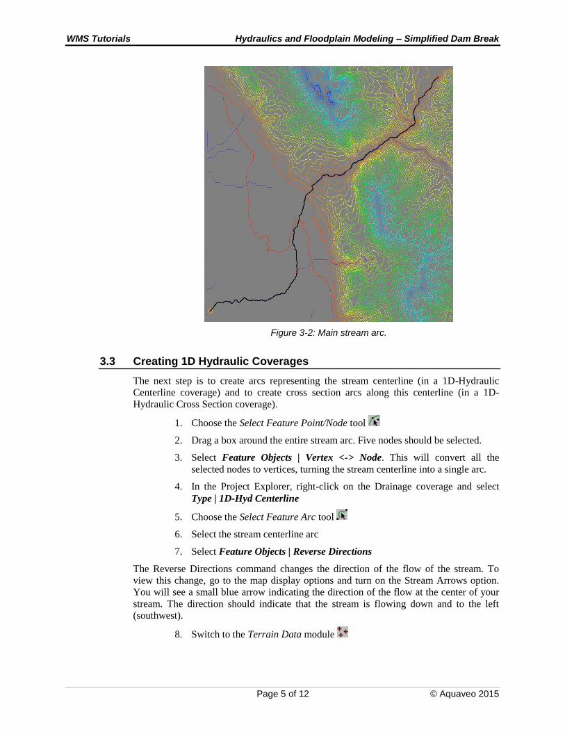
You have now isolated the main stream arc. Your screen should look like Figure 3-2.
WMS Tutorials Hydraulics and Floodplain Modeling – Simplified Dam Break
Page 5 of 12 © Aquaveo 2015
Figure 3-2: Main stream arc.
3.3 Creating 1D Hydraulic Coverages
The next step is to create arcs representing the stream centerline (in a 1D-Hydraulic
Centerline coverage) and to create cross section arcs along this centerline (in a 1D-
Hydraulic Cross Section coverage).
1. Choose the Select Feature Point/Node tool
2. Drag a box around the entire stream arc. Five nodes should be selected.
3. Select Feature Objects | Vertex <-> Node. This will convert all the
selected nodes to vertices, turning the stream centerline into a single arc.
4. In the Project Explorer, right-click on the Drainage coverage and select
Type | 1D-Hyd Centerline
5. Choose the Select Feature Arc tool
6. Select the stream centerline arc
7. Select Feature Objects | Reverse Directions
The Reverse Directions command changes the direction of the flow of the stream. To
view this change, go to the map display options and turn on the Stream Arrows option.
You will see a small blue arrow indicating the direction of the flow at the center of your
stream. The direction should indicate that the stream is flowing down and to the left
(southwest).
8. Switch to the Terrain Data module
WMS Tutorials Hydraulics and Floodplain Modeling – Simplified Dam Break
Page 6 of 12 © Aquaveo 2015
9. Right-click on DEM on the Project Explorer and select Convert | DEM ->
TIN | Filtered
10. Make sure that Triangulate new TIN and Delete DEM options are toggled
on
11. Choose OK
12. In the Project Explorer, right-click on the New tin and select Display
Options
13. In the TIN Data options, toggle off Triangles
14. Select OK
15. In the Project Explorer, right-click on the Coverages folder and select New
Coverage from the pop-up menu
16. Choose 1D-Hyd Cross Section from the Coverage type drop-down box
17. Select OK
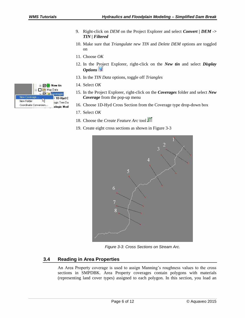
18. Choose the Create Feature Arc tool
19. Create eight cross sections as shown in Figure 3-3
Figure 3-3: Cross Sections on Stream Arc.
3.4 Reading in Area Properties
An Area Property coverage is used to assign Manning’s roughness values to the cross
sections in SMPDBK. Area Property coverages contain polygons with materials
(representing land cover types) assigned to each polygon. In this section, you load an
WMS Tutorials Hydraulics and Floodplain Modeling – Simplified Dam Break
Page 7 of 12 © Aquaveo 2015
existing Area Property coverage. You could also create your own area property coverage
from a background image or map.
1. Select File | Open
2. Open “areaprop.map”
3. Switch to the Map module
4. Choose the Select Feature Polygon tool
5. Double-click on the polygons to view the assigned materials
3.5 Extracting Cross Sections
Once you have completed the centerline, cross section, and Area Property coverages, you
are ready to extract the cross sections from the TIN. Then, you must convert your
coverage data to a hydraulic model.
1. Click on the 1D-Hyd Cross Section coverage to make it the active coverage
2. Select River Tools | Extract Cross Section
3. Toggle on Using arcs and select 1D-Hyd Centerline from the drop-down
list
4. Choose Area Property from the Material Zones drop-down list
5. Select OK
6. Save the file as “xsections”
7. Choose the Select Feature Arc tool
8. Double-click on a cross section
9. Click on Assign Cross Section to view the cross section profile
10. Select Cancel twice to exit the dialogs
11. Click on the 1D-Hyd Centerline coverage to make it the active coverage
12. Select River Tools | Map -> 1D Schematic
4 Using SMPDBK
Setting up your hydraulic model geometry is 90% of the work associated with creating a
SMPDBK model. The other 10% involves entering information about the dam and the
Manning’s roughness values for each of the different area properties. You can find this
information on the Internet or in the National Inventory of Dams (NID) database. This
section will guide you through the process of finishing your SMPDBK model setup.
4.1 Edit Parameters
1. Choose the River module
2. From the Model drop-down box, choose SMPDBK
3. Select SMPDBK | Edit Parameters
WMS Tutorials Hydraulics and Floodplain Modeling – Simplified Dam Break
Page 8 of 12 © Aquaveo 2015
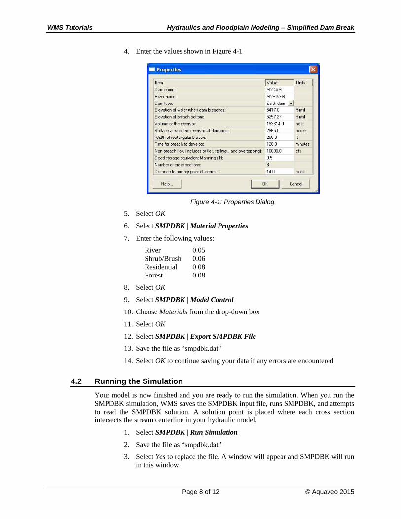
4. Enter the values shown in Figure 4-1
Figure 4-1: Properties Dialog.
5. Select OK
6. Select SMPDBK | Material Properties
7. Enter the following values:
River 0.05
Shrub/Brush 0.06
Residential 0.08
Forest 0.08
8. Select OK
9. Select SMPDBK | Model Control
10. Choose Materials from the drop-down box
11. Select OK
12. Select SMPDBK | Export SMPDBK File
13. Save the file as “smpdbk.dat”
14. Select OK to continue saving your data if any errors are encountered
4.2 Running the Simulation
Your model is now finished and you are ready to run the simulation. When you run the
SMPDBK simulation, WMS saves the SMPDBK input file, runs SMPDBK, and attempts
to read the SMPDBK solution. A solution point is placed where each cross section
intersects the stream centerline in your hydraulic model.
1. Select SMPDBK | Run Simulation
2. Save the file as “smpdbk.dat”
3. Select Yes to replace the file. A window will appear and SMPDBK will run
in this window.
WMS Tutorials Hydraulics and Floodplain Modeling – Simplified Dam Break
Page 9 of 12 © Aquaveo 2015
IMPORTANT NOTE: If you are running on a 64-bit Windows operating system, you will
not be able to run SMPDBK from WMS. You can run SMPDBK from a DOS command
prompt by installing a DOS emulation program such as DOSBOX
(http://www.dosbox.com/) or a similar free product. If you decide to use DOSBOX, after
you start the program, you need to mount the drive(s) where SMPDBK is installed. You
can mount a drive by typing mount C C:\ (for example) if all the files are located on your
C drive. After mounting the drive, just type "C:" to go to your C drive. Then, change to
the directory containing your "smpdbk.dat" file. For example, if your smpdbk.dat file is
located in "C:\Users\aquaveo\Documents\smpdbk", you would type cd
C:\Users\aquaveo\docume~1\smpdbk. Note that the DOS truncates files and folders
containing more than 8 characters to be 8 characters. You can determine the truncated
name by typing dir at the command prompt or just begin typing the name and hit the
TAB key to have the DOS emulator finish the name for you. Once you are in the
directory containing your smpdbk.dat file, you can run smpdbk from a command prompt.
WMS installs smpdbk.exe in the same directory as WMS, so if WMS is installed in
"c:\program files\WMS90\", you would type c:\progra~1\WMS90\smpdbk.exe (note the
truncated name) at the command prompt. Once SMPDBK is started, it asks you several
questions. Make sure your CAPS LOCK key is turned on and type the following answers
for the SMPDBK questions: NO, YES, SMPDBK.DAT, NO, SMPDBK.OUT. A file
called SMPDBK.OUT will be created. You can read this file using the SMPDBK | Read
Solution menu command in WMS. After you have done this, continue on to the Post-
Processing section.
4. Choose Close once SMPDBK finishes running (you may have to wait a
few seconds to a minute or so). If SMPDBK finishes running successfully,
a message such as “Stop—Program terminated” and “SMPDBK Finished”
will appear in the model wrapper.
5 Post-Processing
Once you have finished running SMPDBK, WMS reads the solution as a 2D scattered
dataset. This solution contains water surface elevation points where each cross section
intersects your stream centerline. When you delineate the floodplain, you need additional
solution points to create a well-defined map. This section will guide you through the
processes of interpolating solution points along the centerline and the cross sections.
After interpolating to create additional solution points, you will learn how to delineate the
floodplain from these points.
5.1 Interpolation
1. Click on the 1D-Hyd Centerline coverage to make it the active coverage
2. Select River Tools | Interpolate Water Surface Elevations
3. Select the option to create a data point At a specified spacing (instead of at
each arc vertex).
4. Change the Data point spacing to 1000
5. Select OK
6. Click on the 1D-Hyd Cross Section coverage to make it the active coverage
WMS Tutorials Hydraulics and Floodplain Modeling – Simplified Dam Break
Page 10 of 12 © Aquaveo 2015
7. Select River Tools | Interpolate Water Surface Elevations
8. Select OK
Skip section 5.2 if you are not able to connect to the Internet using your computer.
5.2 Getting a Background Image
Using an Internet connection you can load a background image (Aerial photo or a topo
map) for the project site. You can use any of the Get Data tools in WMS to load images
from the internet.
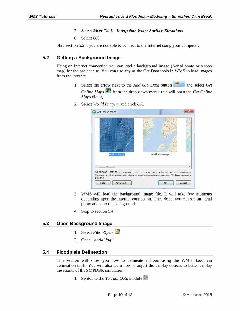
1. Select the arrow next to the Add GIS Data button and select Get
Online Maps from the drop-down menu; this will open the Get Online
Maps dialog.
2. Select World Imagery and click OK.
3. WMS will load the background image file. It will take few moments
depending upon the internet connection. Once done, you can see an aerial
photo added to the background.
4. Skip to section 5.4.
5.3 Open Background Image
1. Select File | Open
2. Open “aerial.jpg”
5.4 Floodplain Delineation
This section will show you how to delineate a flood using the WMS floodplain
delineation tools. You will also learn how to adjust the display options to better display
the results of the SMPDBK simulation.
1. Switch to the Terrain Data module
WMS Tutorials Hydraulics and Floodplain Modeling – Simplified Dam Break
Page 11 of 12 © Aquaveo 2015
2. Select Flood | Delineate
3. Set the Max search radius to 5000
4. Select OK
5. Select MaxWS_fd from the Terrain Data folder of the Project Explorer
6. Right-click on MaxWS_fd and select Contour Options from the pop-up
menu
7. Set the Contour Method to Color Fill and set the transparency to 40%
8. Select the check box for Specify a range
9. Deselect Fill below and Fill above
10. Select the Legend button
11. Toggle on the Display Legend option
12. Select OK two times to exit the dialogs
The flood depths from the SMPDBK simulation can now be viewed as a spatial map.
You will notice that some areas appear flooded that you know are not actually flooded if
the dam breaches. These areas can be corrected by drawing polygons around the areas
you know are not flooded and then re-delineating the floodplain. The following steps
explain how to do this.
13. Right-click on the Coverages folder in the Project Explorer and select New
Coverage from the pop-up menu
14. Choose Flood Barrier from the Coverage Type drop-down box
15. Select OK
16. Choose the Create Feature Arcs tool
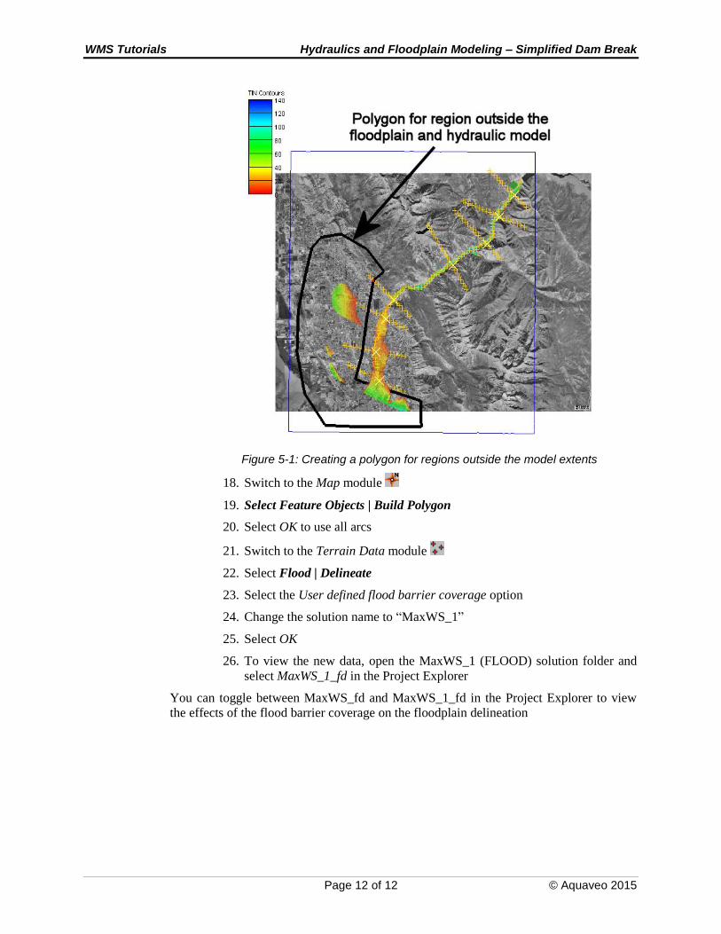
17. Draw an arc representing a polygon around the extra data that needs to be
deleted. This includes areas clearly outside of the floodplain and areas
where data does not exist to give accurate results, such as outside the
extents of the hydraulic model (see Figure 5-1). WMS will ignore the areas
inside this polygon when delineating your floodplain. Be sure your arc
forms a closed loop.
WMS Tutorials Hydraulics and Floodplain Modeling – Simplified Dam Break
Page 12 of 12 © Aquaveo 2015
Figure 5-1: Creating a polygon for regions outside the model extents
18. Switch to the Map module
19. Select Feature Objects | Build Polygon
20. Select OK to use all arcs
21. Switch to the Terrain Data module
22. Select Flood | Delineate
23. Select the User defined flood barrier coverage option
24. Change the solution name to “MaxWS_1”
25. Select OK
26. To view the new data, open the MaxWS_1 (FLOOD) solution folder and
select MaxWS_1_fd in the Project Explorer
You can toggle between MaxWS_fd and MaxWS_1_fd in the Project Explorer to view
the effects of the flood barrier coverage on the floodplain delineation


