
1
CESIS Electronic Working Paper Series
Paper No. 11
Sources of Finance, R&D Investment and Productivity: Correlation or Causality? 1
Almas Heshmati and Hans Lööf
(CESIS, INFRA)
First version September 2004, Revised version June 2005.
The Royal Institute of technology Centre of Excellence for Science and Innovation Studies
http://www.infra.kth.se/cesis/research/workpap.htm Corresponding author: [email protected]

2
Sources of Finance, R&D Investment and Productivity: Correlation or Causality?
Almas Heshmati♦ and Hans Lööf∗
First version September 2004, Revised June 2005
Abstract
In general there is an agreement about the positive impacts of R&D on performance of firms
measured as productivity growth, profitability and growth. However, the opposite relationship
is less obvious and very little attention has been paid on examining the feedback from
performance on R&D investment. This study contributes to the empirical analysis of a two-
way causal relationship between R&D investment and performance at the firm level. We
examine the interaction between a number of financial indicators represented by investments
in R&D and tangible capital and a number of performance variables including sales, value
added, profit, cash flow, capital structure and employment. Empirical results are based on a
large panel data set of Swedish manufacturing firms over the period 1992-2000. The results
show evidence of weak feedback effects from performance on investment.
Keywords: R&D investment, productivity, financial constraints, panel data
JEL Classification: C23, C33, G32, L19, O33
♦ Corresponding author: Almas Heshmati, Techno-Economics Policy Program, College of Engineering, Seoul National University, San 56-1 Shinlim-dong Kwanak-gu, Bldg #38, Seoul 151-742, Korea, E-mail: [email protected] ∗ Centre of excellence for Science and Innovation Studies, Royal Institute of Technology, Stockholm Sweden, Teknikringen 78, 100 44 Stockholm, Sweden, E-mail: Hans.Löö[email protected]. We are grateful to Bronwyn Hall for her encouragement, comments and suggestions.
3
1. INTRODUCTION
It the economic literature it is well recognized that R&D makes a vital contribution to the
level of productivity (Cohen and Klepper, Griliches, 1998, Sutton, 1998).1 However, the
innovation and growth literature still lack robust empirical evidence on a possible reverse link
from productivity to the R&D activities. A priori it can be assumed that such a relationship is
very likely to exist. The presence of a reversal link is suggested by several economists.
Baumol and Wollf (1983), and Pakes and Griliches (1984) are among the pioneering
contributors. Firm performance affects the availability of internal resources through retained
profits. It improves also access to external resources through securities for investments in
general and for investments in R&D in particular.
This study contributes to the lacking empirical analysis of the two-way causal relationship
between investment and performance at the firm level. We examine the interaction between a
set of financial indicators represented by investments in R&D and tangible capital and a set of
performance variables including sales, value added, profit, cash flow, capital structure and
employment. The objective is to shed lights on the concerns about the above causality
relationship by using new data and new estimation methods that account for potential biases
induced by simultaneity, omitted variables, and unobserved firm-specific heterogeneity
effects that can bias the analysis of the link between investment and growth. Empirical results
are based on a large panel data set of Swedish manufacturing firms over the period 1992-
2000. The results show evidence of a weak feedback effects from performance on investment.
Methodologically the paper uses several different approaches including simple cross-sectional
instrumental variable regressions aiming to serve as a benchmark for the panel data analysis.
In the causality part we compare results from pooled models including fixed effects models
accounting for firm-specific effects and allowed to be correlated with explanatory variables.
In addition the variables are expressed both in intensity, i.e. per employee, as well as per firm
levels. Furthermore, we compare investment in tangible and intangible assets.
We compare our results with findings on the issues of causality presented in Mairesse and
Hall (1996), Hall, Mairesse, Branstatter and Crepon (1998), Bond, Harhoff and Van Reenen
(1999), Levine, Loayza and Beck (2000), Gholami, Tom-Lee and Heshmati (2003), and
others. Our approach is an improvement of approaches employed in previous studies listed in
above by applying a multivariate approach on an extensive data set. Thereby, it strengthens 1 Productivity here refers to set of indicators such as value added or sales per employee.
4
the evidence on the dynamic relationship between finance, investment and growth. We are
using a panel data version of the Vector Auto Regressive (VAR) methodology for testing the
causal relationship between indicators/measures of financial performance on one side and
investment in tangible and intangible assets on the other side.
Rest of the paper is organized as follows. The next section presents a brief review of findings
from the recent literature on financial constraints and investment at the firm level. Section 3
describes the data used. In Section 4, the empirical model along with estimation procedures is
discussed. Results from empirical analysis of causality relationship from application of
various cross-sectional and panel data approaches are presented in Section 5. Final section
concludes this study and provides guidelines for future studies of causal relationship between
performance and investment.
2. FINANCING INNOVATION
Corporate governance and financial institutions play an important role to the way that firms’
investment decision and industrial dynamics might have impacts on firms’ performance. For
pioneering contributions on this issue see Schumpeter (1942), Nelson (1959) and Arrow
(1962). The efficiency of the financial system to distribute and reallocate resources to the
economy’s most productive users is an important driving force to Schumpeterian waves of
creative destruction and economic growth. The capacity to channel resources to young and
dynamic firms with growing potential and to R&D-intensive firms is identified to be of
particular importance.
For the American economy, Hall (2002) finds that the capital structure of R&D intensive
firms customarily exhibits less leverage than that of other firms. The reasons is that banks
and other debt holders prefer to use physical assets to secure loans and are reluctant to lend
when projects involves substantial R&D-investments. As a consequence, external financing
will be relatively more expensive for R&D investment than for normal investment suggesting
a close relationship between firms’ performance such as profit, productivity or cash flow on
the one hand and their R&D investment decisions on the other.
Partly influenced by recent improvements in econometric modeling of causal relationships by
Holtz-Eakin, Newly and Rosen (1988, 1990), the Arellano and Bond (1991), and Blundell and
Bond (1998) these approaches have increasingly been used in different areas of economic
analysis. Investigating the relationship between stock markets, banks and growth, Rousseau
5
and Wachtel (2000) use a difference panel data estimator to omitted variable bias and
simultaneity bias and report that both banking sector and stock market development explains
subsequent growth, even after controlling for reverse causality. Gholami, Tom-Lee and
Heshmati (2003) apply Granger causality test and explored the simultaneous causal
relationship between investment in information and communication technology (ICT) and
inflow of foreign direct investment (FDI). They report that in developed countries the existing
ICT infrastructure attracts FDI, while the direction of causality goes the other way around in
developing countries.
Hall, Mairesse, Bransetter and Crepon (1998) contributed to the innovation and growth
literature by applying the Holz-Eakin influenced Newly and Rosen (1990) methodology on
cross-country data sets in evaluating whether cash flow and sales cause physical investment
and R&D. The main findings show that the direction of causality differs between the
investigated countries, suggesting the importance of institutional differences between the
“market based” Anglo-Saxon countries (United States, United Kingdom and Canada) and the
“bank-based” financial systems such as those of France, Germany and Japan.
3. THE DATA AND DESCRIPTIVE STATISTICS
Having reviewed the literature on financing innovation this section presents the innovation
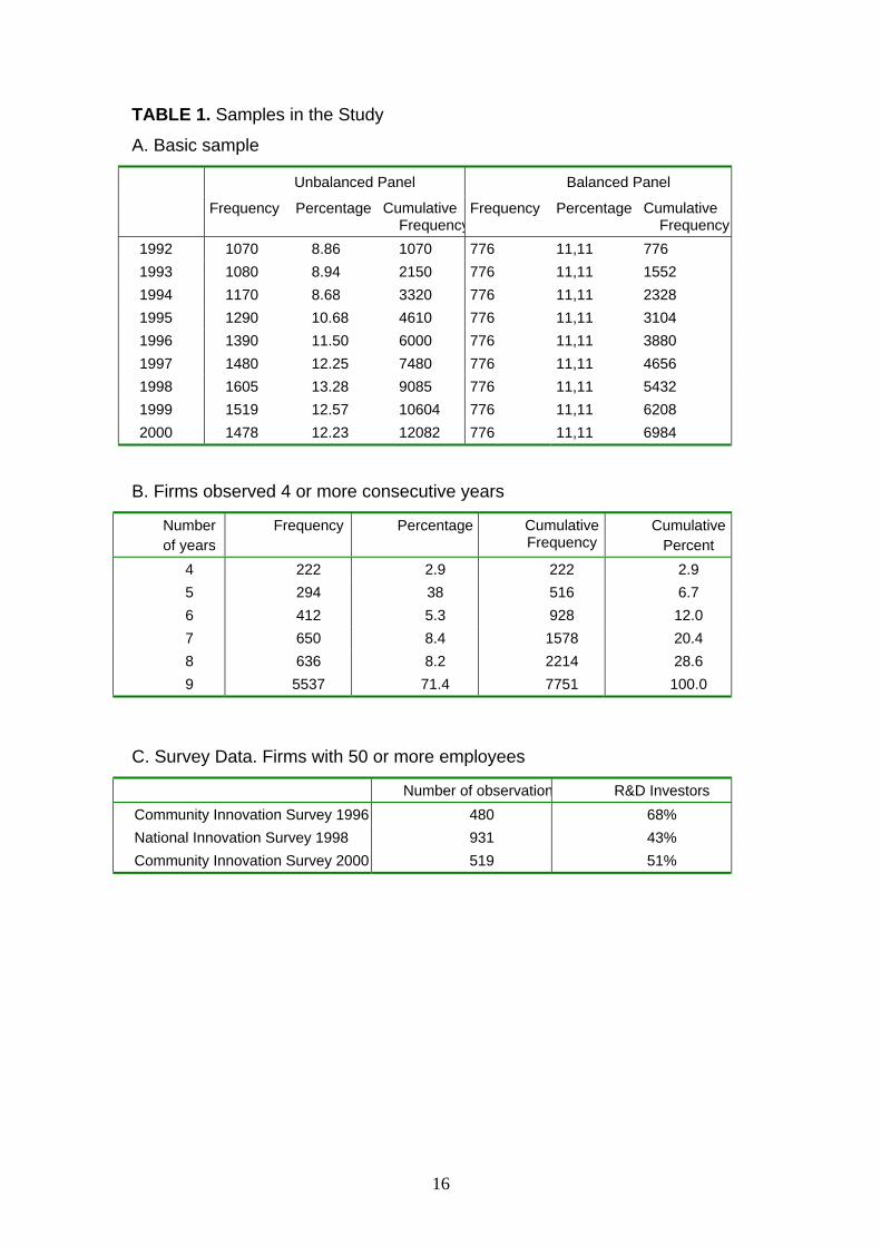
data used in the empirical analysis. In Table 1 we present summary of the sample of
manufacturing firms used in the paper. The point of departure for the study is three
consecutive Community Innovation Surveys (CIS) conducted in Sweden in 1996, 1998 and
2000 (for details see Panel A of Table 1). In order to merge the survey sub-samples with
register data containing R&D information the final data is restricted to firms with 50 or more
employees. This results in 480, 931 and 519 observations respectively for the three periods
and sub-samples. It should be noted that these three series are only partially overlapping. For
each of these sub-samples we have access to register data covering the entire period of 1992-
2000. However, finally we only use the panel data based on the richest data set namely the
1998-survey. It should be noted that samples are stratified and the resulting data here
correspond to more than 75% of all the existing manufacturing firms in Sweden with 50 or
more employees.
In Table 1, panel B we show summaries of both unbalanced and balanced versions of the data.
The former consists of 12,082 observations while the latter 6,984 observations. Since, we use

6
lag variables to establish causal relationship between the variables of interest, the unbalanced
panel consisting of firms observed at least 4 consecutive years is reduced to 7751
observations (see Panel C of Table 1). The unbalanced panel, despite increased data
management and estimation complications, is of course preferred as it allows for both entry
and exit of firms to the market and it has the advantage that it allows to avoid sample
selection bias.
The key variables in the panel data analysis are presented in Table 2. The financial
performance variables include sales, value added, gross profit, cash flows and capital structure
or degree of indebtedness. The investment variables are represented by investment in tangible
assets and R&D investments. In analyzing causal relationship between the two sets of
financial performance and investment variables we control for human capital measured as
share of employment with a university degree and the knowledge intensive technology used at
the firm level.
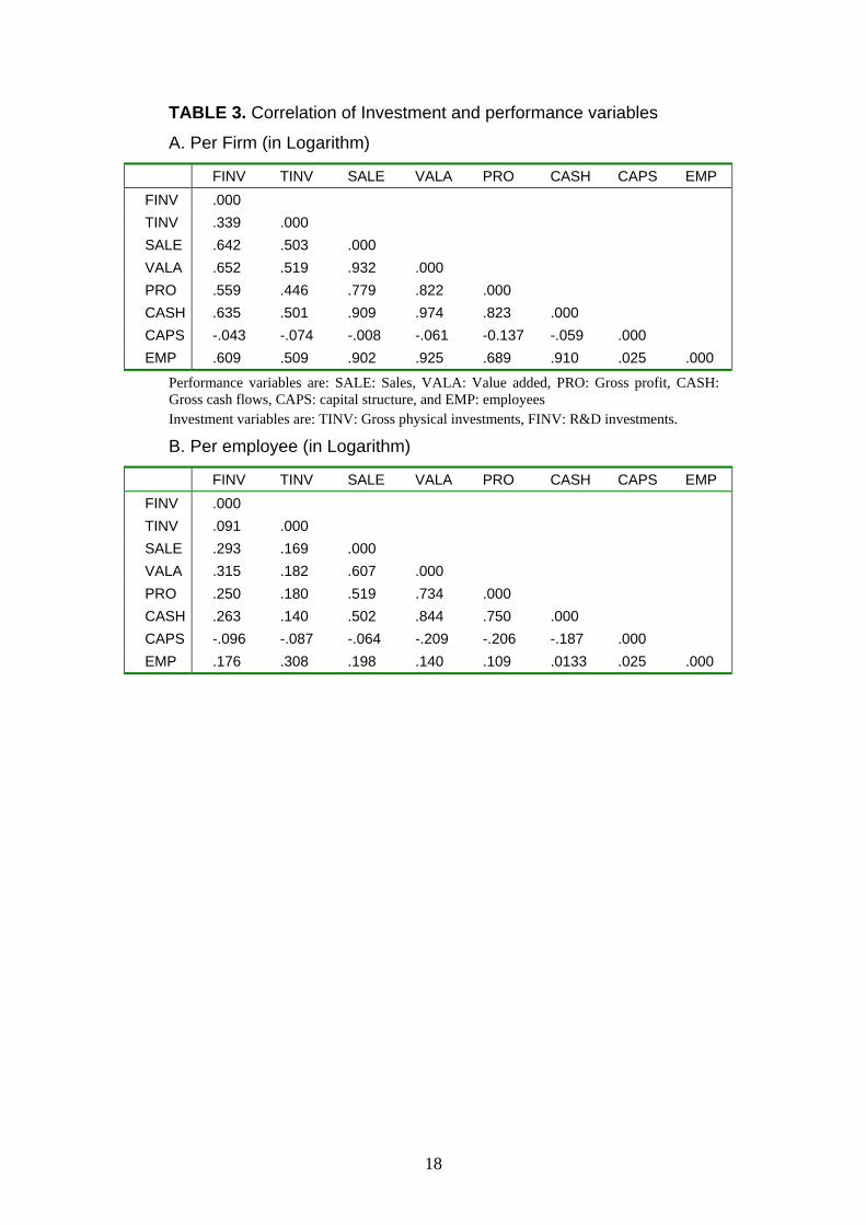
The correlation between investment variables and financial performance variables measured
at firm and per employee levels are shown in Table 3. Starting with Panel A of Table 3, sales,
value added and cash flows exhibit high correlation with R&D investment. The correlation
between these three financial variables and investment is somewhat lower when we substitute
R&D for investment in tangible assets. Capital structure measured as the ratio of debt to sum
of debt and equity is negatively associated to both types of investment. The correlation
coefficients for variables measured in form of intensity, i.e. per employee shows a similar
pattern as the aggregate firm level, but considerably with lower level of correlation.
4. THE EMPIRICAL MODEL AND ESTIMATION PROCEDURES
While overwhelming evidence show that R&D is a good predictor of productivity most results
do not take into account the issue of causality. However, systematic testing and determination
of causal directions become possible after Granger (1969) and Sims (1972) developed an
operational framework. Stylized Facts on R&D, productivity and innovation based on robust
Empirical evidence from the literature are as follows2:
R&D-investments and Productivity
• At the between firms, R&D and of productivity are positively related
2 See more details see Cohen and Klepper (1996) and Klette and Kortum (2002).

7
• At the within-firms, across-time R&D and growth rate of productivity are
unrelated.
R&D investments and Innovation
• Level of R&D (flow) and level of innovation output (measured as patent and sales)
across firms are positively related
• There are diminishing returns to R&D in the longitudinal dimension
• Performing R&D on a permanent basis is positively related to innovation output
However, the existence of a relationship between the variables in above does not prove
causality or the direction of influence. To explain the granger test for causality, we will
consider the question: Is it R&D that “causes” the increased productivity )( yx → or is it the
increased productivity that causes R&D )( xy → . A variable x is said to Granger causes a
variable y if, given the past values of y, past values of x is useful in predicting y. The Granger
causality (Granger 1969) test assumes that the information relevant to the prediction of the
respective variables, R&D and productivity, is contained solely in the time dimension of the
data on these variables.
A common method for testing Granger causality is to regress the variable y on its own lagged
values and on lagged values of x variable, and to test the null hypothesis that the estimated
coefficients on the lagged values of x are jointly zero. Failure to reject the null hypothesis is
equivalent to failing to reject the null hypothesis that x does not Granger causes y. It should
be noted that in testing for causal relationship between two or more variables one could
account for heterogeneity (labelled as z-variables) not reflected in the lag of variables of
interest. The test involves the estimating of the following pairs of variables:
(1) tjtj
n
j
iti
n
i
t uYDRY 1
11
& ++= −
=
−
=∑∑ βα
(2) tjtj
n
j
iti
n
i
t uYDRDR 2
11
&& ++= −
=
−
=∑∑ γλ
where it is assumed that the disturbances tu1 and tu2 are uncorrelated. For the panel data
analysis we will apply the Granger causality test and examine presence of a two-way causal
relationship based on estimation results where the models are estimated jointly using least
square method applied to pooled data as well within estimation method accounting for
8
unobservable firm-specific effects. Moreover, for the reasons of sensitivity analysis of the
results we will also compare results based on variables expressed in intensity (per employee)
and also in non-intensity (firm level) terms, as well as cases where investment is decomposed
into tangible and intangible capital components.
In order to check the robustness of the panel data we will employ an instrumental variable
version of the so-called Crepon, Duguet and Mairesse (1998) known as CDM- model on data
from three consecutive innovation surveys. The model consists of four equations. In this four-
equation model we introduce financial variables in forms of profit, equity and debt in the
R&D equation.3
5. EMPIRICAL RESULTS
5.1 Instrumental variables estimates
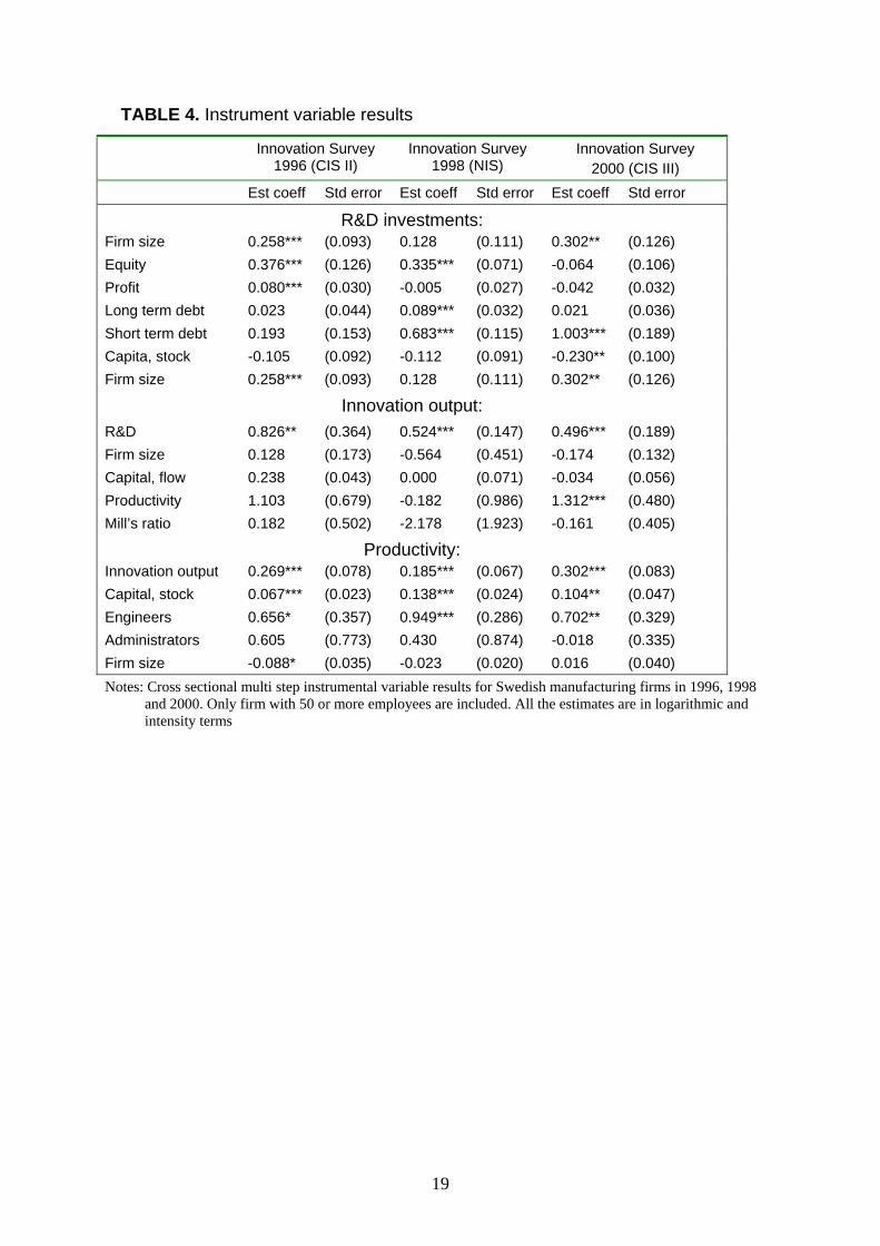
The results from testing for causal relationship between R&D investment and performance
variables including innovation output and productivity are reported in Table 4. The results are
organized in the following way. The top panel shows the R&D equation for the three cross
sectional consecutive CIS innovation surveys. The middle panel presents the innovation
output estimates for each survey separately. Finally, the bottom panel shows the productivity
equation again separately for each sample survey. The key finding can be summarized as
following: (i) the main estimation results are consistent with those reported in previous studies
using different versions of the CDM-model in a cross sectional framework, (ii) introducing
information on equity, debt and profit from register data in the R&D equation reveals some
contradictory results.
In considering first the CIS survey II from 1998 results to the left side of the table, we find
that equity as well as profit has a positive and highly significant impact on R&D investment.
On the contrary, neither the long term debt nor short term debt is associated with R&D effort.
A tentative conclusion is that firms prefer to finance R&D by retaining earning or through the
stock market. This pattern is consistent with what we a priori would expect to find based on
both theoretical and empirical literatures of liquidity constraints and corporate governance 3 The model consists of four equations including: propensity to invest in innovation activities, innovation input, innovation output and productivity. The first two equations are estimated using generalized tobit model, while the last two equations are estimated in a simultaneous equations system. The estimation procedure accounts for both selectivity and simultaneity biases. For details on the specification and estimation of the model, see Lööf and Heshmati (2002 and 2005).
9
(See, Hall (2002) for a recent review of the literature). However, the middle part of the Table
4 shows a close correlation between our both debt measures and R&D-investment. Still the
equity variable is positive and highly significant, but using the year 1998 observations, we
find no relationship at all between profit and intangible investments. Finally, the right hand
side of Table 4 (based on CIS survey III related to year 2000), exhibits negative estimates for
both equity and profit, however they are statistically insignificant. For the average
manufacturing firm with 50 or more employees, observed in the CIS-survey, R&D-investment
per employee increases with short-term debt, while we find no significant relationship
between long-term debt and R&D investment.
The puzzling results reported in the three different cross-sectional R&D-equations of the first
step of the CDM-model indicate the importance of using a dynamic approach when analyzing
the determinants R&D. In the following we will rely on panel data methodology to establish
the causal relationships outlined in above and they are derived from following up the selected
sample in the year 1998 innovation survey for the period 1992 to 2000. The choice of period
of study is determined by data availability.
5.2 Forward and backward development of the data
Table 5 gives simple description of the merged CIS and register data covering 1992-2000.
Here by forward we mean that the CIS survey used as bases for merging the innovation
survey with register data is the innovation survey in 1992. The sample firms observed in 1992
are then followed forward until year 2000. For the backward the sample used as bases for the
merging of innovation and register data is the innovation survey from year 2000. These firms
are then followed backward until 1992. For the third sample observed in 1998 the sample
firms are followed up both forward and backward covering 1992-2000. We compare the
development of the key variables by R&D intensity both forward and backward by using
1998 as reference point.
The sample is divided into three subgroups distinguished by the size of investment: zero
investment, moderate R&D investment rate (0.1-2.0% as a share of sales) and high investment
rate (more than 2%). The left hand side of the Table 5 shows that the initial R&D intensity is
a fairly good predictor of the growth rate of sales, value added, profit, cash flows and
employment during 1992-2000. The growth rates of all of these five performance indicators
were highest for the R&D intensive sub-sample and lowest for the non R&D firms. The

10
growth rate of debt was considerably lower for R&D intensive firms with investment rate
exceeding 2% of their sales compared to the two other groups of firm.
In looking backward with reference to 1998, the right hand part of Table 5 starts from year
2000 and follows the firms back until 1992. With the exception of the growth rate of
employment the backward expanded data shows similar pattern as the forward expanded data:
The growth rate of profit, sales, value added and cash flows during 1992-2000 increases with
the year 2000 R&D-intensity, and the growth rate of equity and debt per employee decreases
with R&D intensity. The annual growth of employment was not related to R&D intensity.
5.3 Multivariate Granger causality tests
In investigation of the causal relationships between investment and financial variables at the
firm level in a cross-sectional framework dimension and application of a bivariate framework
Hall et al. (1998) report mixed results when the lags variables chosen are 1-4 years. The
present analysis is an extension of the Hall et al. study in the sense that we are conducting a
multivariate analysis and also include some additional performance measures to the
specification.
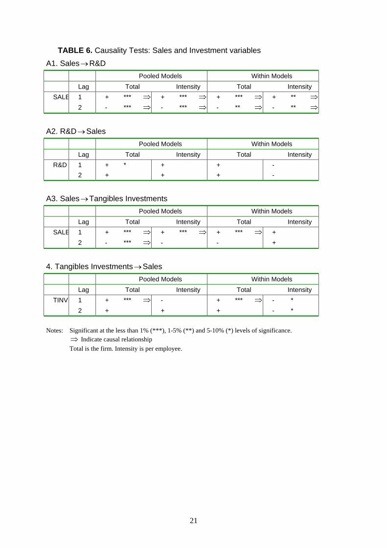
Table 6 presents the summary of results of the causality tests for three performance measures
namely, sales, employment and profitability and two investment measures of tangible and
intangible assets. In Panels A to D of Table 6 the main finings are shown for pooled models
and those estimated with within estimation method, further divided into results based firm
level and per employee levels data. It is to be noted that here we have chosen to use two lags.
The data is unbalanced and allow for entry and exit of firm to the market. The minimum
number of years required for a firm to be observed consecutively due to the used lagged
variables is set to 4 years.
Causality test results reported in Panel A1 and A3 of Table 6 indicate that both R&D-
investment and physical investment are highly sensitive to the level of lagged sales. However
the sign of the coefficient estimates for sales alters. It changes from positive to negative when
two lags are considered.
Panel A2 and A4 of Table 6 display the causal effect from investment to sales. Somewhat
unexpectedly both of the pooled model and the within model results show evidence of a weak
feedback effect from R&D to sales. Considering the tangible investment both models shows
highly significant and positive influence from tangible investment when our measurement unit
11
is the firm level and numbers of lags are 1. Otherwise we find that no causal relationships can
be established between investment and sales variables.
In Table 6B the causality tests between profitability and investments are reported. Looking
first at the two upper panels we see different patterns between pooled and within models. The
pooled model results shows that profit Granger causes R&D when 1 lag is considered, and
that 2 lags of R&D causes profitability. The within models results are all insignificant at the
les than 5% levels of significance. The lower part of Table 6B shows that profitability
typically causes tangible investments, however the impact from tangible investments on
profitability is more mixed. One lag of tangible investment has a significant negative
influence on profitability, while two lags of tangible investments Granger causes profitability
in the pooled models. The within models results are statistically insignificant.
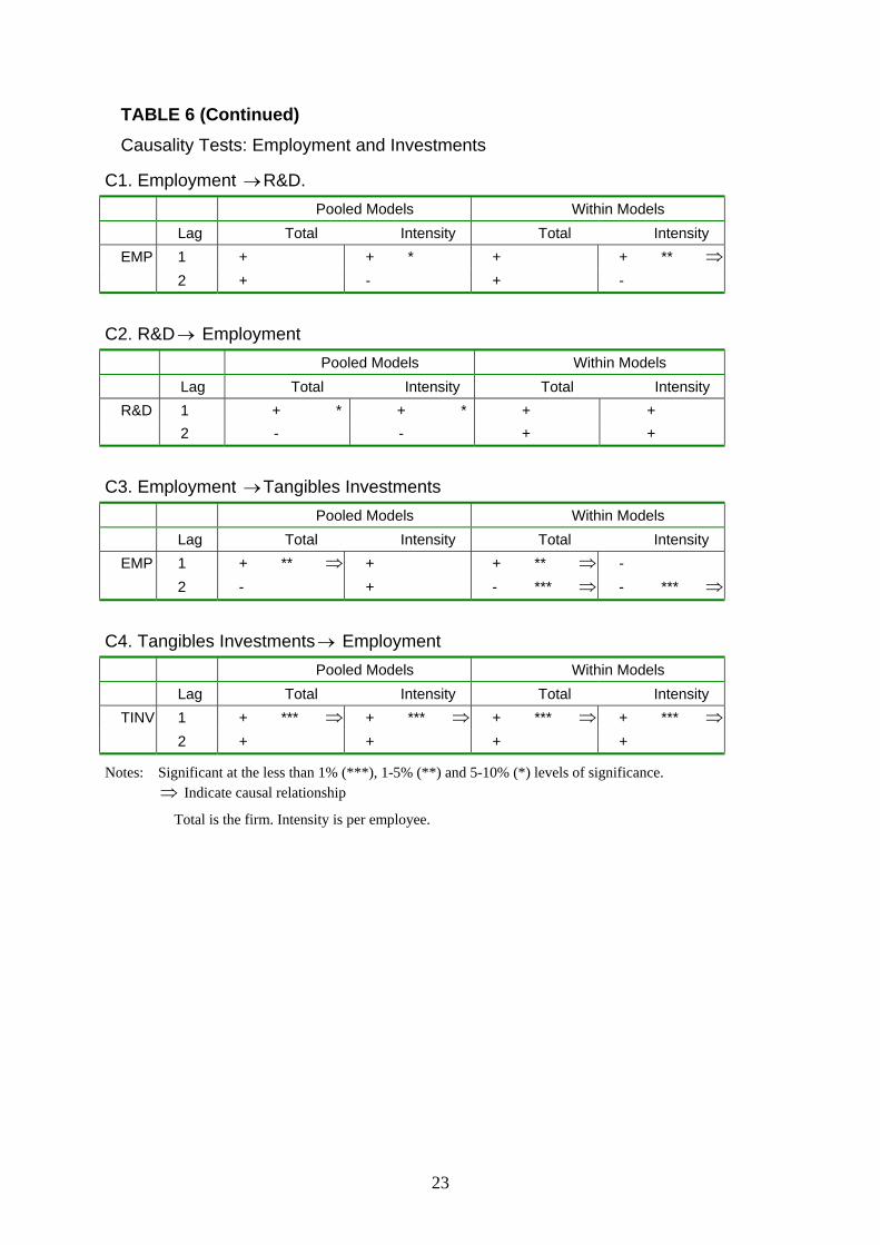
The results in Table 6C show that the relation between R&D and employment which typically
is positive in both directions but each one turned out statistically insignificant. On the contrary
the results here indicate that tangible investment causes growth in employment.
The upper part of Table 6D revels that tangible investments have a negative impact on R&D
in the short run (when using 1 Lag) indicating presence of financial constraints. In the 2-lag
perspective, however the feedback effect from physical investment on R&D is positive but
only significant in the pooled model case.
Panel D2 of Table 6 shows that R&D-investment has positive but insignificant impact on
tangible investment.
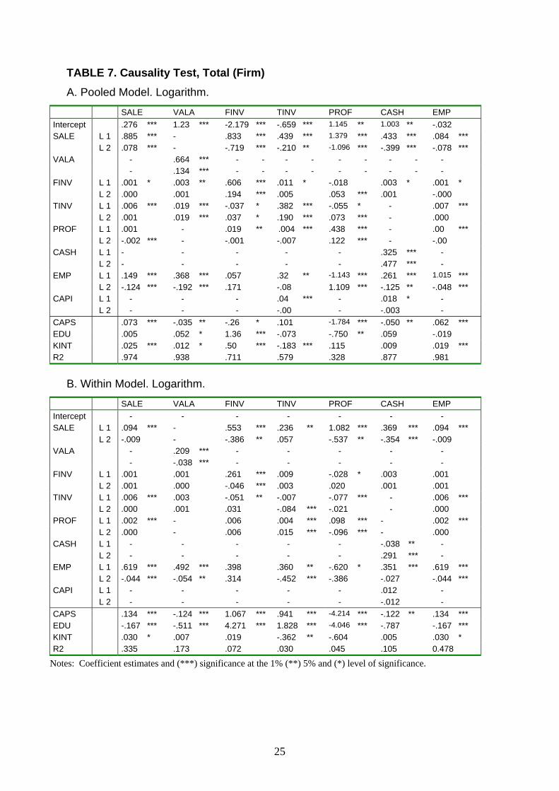
5.4 The full model results
Table 7 provides detailed information on the multivariate causality results partly summarized
in different parts of Table 6. In sum the regression results for 7 different equations are
reported. Panel A and Panel B show results for aggregate firm level data using pooled and
within models, respectively. Panel 7C and Panel 7D display the pooled and within models
results where the variables are measured in intensity or per employee terms.
Not surprisingly, all seven dependent variables (5 firm performance variables and 2
investment variables) show a strong and highly significant relationship with their own lag
variables, however the signs are mixed. The pooled model confirms the findings by Hall
(2002) on a negative association between capital structure and R&D-investments. However in
12
the within models the relationship is positive and highly significant. The explanation for the
latter might be found in the large differences between the financial markets in the U.S. and
Sweden (see also Lööf, 2004) as well as the share of the total variations divided into with and
between components.
The education variable (measured as share of the employment with university degree) which
serves as a proxy for human capital is strongly correlated with R&D-investment and one may
suspect endogeneity problem between these two variables.
The results in Table 7 display quite weak predictive power of R&D for sales, value added,
profit, employment and physical investment and the reverse causal influence is also typically
not found to be strong.
6. CONCLUSIONS
Does a better financial performance of firms exert a positive influence on their R&D
investments? While previous research in this area have shown that the level of R&D is a good
predictor of financial performance across firms, they are far from being able to establish the
nature of causal relationships between the key investment and performance variables. The
well documented (see e.g., Klette and Kortum 2002) fragile and typically insignificant
relationship between firms’ (within-firm, across time) R&D and their productivity growth
suggest that the issues of causality is of great importance to economists in their evaluation as
well as for policymakers in their decisions.
This paper first examined the cross-sectional nature of the R&D and firm performance
relationships. The empirical results are based on data from three consecutive Swedish
innovation surveys and using a common multi-step estimation approach which accounts for
both simultaneity and selection biases. As expected the results showed evidence of a strong
and highly significant relationship between R&D and productivity through innovation output
measured as share of sales associated with new product and processes.
Next we conducted the time dimension analysis by a simple forward backward analysis and
found that R&D is a good predictor of future growth in foremost profit and employment, but
also sales, value added and cash flows. Moreover, no R&D or only moderate R&D intensity
predicts growing debt. The backward analysis indicate that the growth rate of profit, value
added and sales are fairly good predictors on future R&D-intensity, while the growth rate of

13
both equity and debt is negatively related to the future R&D-intensity. The capital stock is
found to be neutral to R&D in the simple descriptive statistical forward and backward
analysis.
In the Granger causality analysis we conducted causality tests based on both pooled and
within estimation analysis. We compared the results for the key variables with regards to
measurement in form intensity (per employee) as well as the average manufacturing firm
levels, and we also explored different performance measures and the two main types of
investment; the tangible and intangible investments.
The results suggest a large and highly significant causal influence from sales to R&D but not
the reverse causality. The feedback on R&D from profit is mostly positive, however only
weakly significant or in some cases statistically insignificant. The causal relationship between
employment and R&D turned out to be fragile and statistically insignificant.
Somewhat unexpectedly our results revealed a stronger association between tangible capital
and profit, and tangible capital and employment, than was expected between R&D and profit
and R&D and employment, respectively. Considering the both categories of capital we found
a stronger impact on R&D from physical investment than the reserve causal effect.
We find it important to conclude this study with a few suggestions for future research on the
causality between R&D investment and performance. One import step is to extend the
relatively short panel data to a longer time period. This gives a better base for applying system
of equations and alternative estimation methods such as Generalized Methods of Moment
(GMM) for dynamic panel data analysis. Another extension is to perform stationarity tests in
the data sets prior to the causality tests. Unfortunately none of these extensions are possible
by the current data sets with short time coverage.

14
REFERENCES
Arellano, M. and S. Bond (1991), Some test of specification for panel data: Monte Carlo
evidence and application to employment equations, The Review of Economic Studies
58: 277-97.
Arrow, K. J. (1962), Economic Welfare and the Allocation of Resources for Invention, In
Richard Nelson (ed.), The Rate and Direction on Inventive Activity. Princeton, N.J.:
Princeton University Press.
Baumol, W, and E. Wolff, (1983), Feedback from Productivity Growth to R&D,
Scandinavian Journal of Economics, 85 (2).
Blundell, R. S., and S. Bond (1998), Initial Conditions and Moment Restrictions in Dynamic
Panel data Models, Journal of Econometrics 87: 115-143.
Bond, S., D. Harhoff, and J Van Reenen. (1999), Investment, R&D and Financial Constraints
in Britain and Germany. Institute of Fiscal Studies Working Paper no 99/5.
Brown, W. (1997) R&D Intensity and Finance: Are Innovative Firms Financially
Constrained? London School of Economics Financial market Group.
Cohen, W and S. Klepper (1996), A reprise of size and R&D. Economic Journal, 106, 925-
51.
Crépon, B., E. Duguet and J. Mairesse (1998), Research, Innovation, and Productivity: An
Econometric Analysis at the Firm Level, NBER Working Paper No. 6696.
Granger, C. W. (1969), Investigating causal relations by econometric models and cross-
spectral methods, Econometrica 37 (3): 424-38.
Griliches, Z. (1998), R&D and Productivity. The Econometric Evidence. The University of
Chicago Press.
Gholami, R., Tom-Lee S-Y. and A. Heshmati (2003), The Causal
Relationship Between Information and Communication Technology and Foreign
Direct Investment, WIDER Discussion Paper 2003:30.
Hall, B. H., J. Mairesse, L. Branstetter, and B. Crepon (1999), Does Cash Flow Cause
Investment and R&D: An Exploration using Panel Data for French, Japanese, and
United States Firms in the Scientific Sector, in: Audretsch, D, and A. R. Thurik (eds.),
Innovation, Industry Evolution and Employment. Cambridge, UK: Cambridge
University Press.
Hall, B. H. (2002), The Financing of Research and Development, NBER No 8773.
Holtz-Eakin, D., W. Newey and H. Rosen (1990), Estimating Vector Autoregressions with
Panel data, Econometrica 56, 1371-95.

15
Klette, T.J. and S. Kortum (2002), Innovating Firms and Aggregate Innovation, NBER
Working Paper 8819.
Levine, R,. N Loayza, and T. Beck (2000), Financial Intermediation and Growth: Causality
and Causes, Journal of Monetary Economics, 46, 31-77.
Lööf, H. (2004), Dynamic Optimal Capital Structure and Technical Change, Structural
Change and Economic Dynamics 15(4), 449-468.
Lööf, H., and A. Heshmati (2005), On the Relationship Between Innovation and
Performance: A Sensitivity Analysis, Economics of Innovation and New Technology,
forthcoming.
Mairesse J., and B.H. Hall (1996), Estimating the Productivity of Research and Development
in French and United States Manufacturing Firms: An Exploration of Simultaneity
Issues with GMM, in: van Ark, Bart and Karin Wagner (eds.), International
Productivity Differences, Measurement, and Explanations. Amsterdam:
Elsevier_north-Holland.
Nelson, R. R. (1959), The Simple Economics of Basic Science Research, Journal of Political
Economy 49, 297-306.
Pakes, A. and Z. Griliches (1984), Patents and R&D at the Firm Level. A First Look. In
Griliches (ed), R&D, patents, and productivity. Chicago: University of Chicago Press.
Rousseau, P. L. and P. Wachtel (2000), Equity Markets and Growth: Cross-Country Evidence
on Timing and Outcomes, 1980-1995, Journal of Business and Finance, November
2000, 24: 1933-57.
Sims, C. (1972), Money, Income and Causality, American Economic Review 62: 540-52.
Sutton, J. (1998), Market Structure and Technology. Cambridge, Mass. MIT Press.
Schumpeter, J.A. (1911) The Theory of Economic Development. Cambridge, MA: Harvard
University Press.
Schumpeter, J.A., (1942), Capitalism, Socialism and Democracy, New York: Harper and
Row.
16
TABLE 1. Samples in the Study
A. Basic sample
Unbalanced Panel Balanced Panel
Frequency Percentage Cumulative Frequency
Frequency Percentage Cumulative Frequency
1992 1070 8.86 1070 776 11,11 776 1993 1080 8.94 2150 776 11,11 1552 1994 1170 8.68 3320 776 11,11 2328 1995 1290 10.68 4610 776 11,11 3104 1996 1390 11.50 6000 776 11,11 3880 1997 1480 12.25 7480 776 11,11 4656 1998 1605 13.28 9085 776 11,11 5432 1999 1519 12.57 10604 776 11,11 6208 2000 1478 12.23 12082 776 11,11 6984
B. Firms observed 4 or more consecutive years
Number of years
Frequency Percentage Cumulative Frequency
Cumulative Percent
4 222 2.9 222 2.9 5 294 38 516 6.7 6 412 5.3 928 12.0 7 650 8.4 1578 20.4 8 636 8.2 2214 28.6 9 5537 71.4 7751 100.0
C. Survey Data. Firms with 50 or more employees
Number of observation R&D Investors Community Innovation Survey 1996 480 68% National Innovation Survey 1998 931 43% Community Innovation Survey 2000 519 51%

17
TABLE 2. Summary statistics of the variables
Variable Mean Std. Dev Min Max
SALE 100 0.0 100 100 VALA 36.5 12.1 0.1 86.7 PRO 6.0 7.8 -80.9 71.6 CASH 36.2 12.3 0.0 100 CAPI 23.4 22.6 0.0 658.8 DEBT 43.3 36.7 1.0 1185.5 EQUI 20.0 26.7 -23.1 713.2 TINV 4.9 8.1 0.0 334.7 FINV 1.3 3.1 0.0 52.9 CAPS 70.9 19.3 5.1 100 EDU 14.1 10.8 0,0 77.6 KINT 29.1 45.5 0.0 100
Notes: Definition of the variables. SALE: Sales, VALA: Value added, PRO: Gross profit, CASH: Gross cash flows, CAPI: Physical capital, DEBT: Total dent, EQUI: Equity, TINV: Gross physical investments, FINV: R&D investments, CAPS: Capital structure (debt/(debt+equity)), EDU: Share of the employee with university degree, KINT: Share of knowledge intensive firms.
With the exception of education and knowledge intensity all other variables are expressed as share of sales.
18
TABLE 3. Correlation of Investment and performance variables
A. Per Firm (in Logarithm)
FINV TINV SALE VALA PRO CASH CAPS EMP FINV .000 TINV .339 .000 SALE .642 .503 .000 VALA .652 .519 .932 .000 PRO .559 .446 .779 .822 .000 CASH .635 .501 .909 .974 .823 .000 CAPS -.043 -.074 -.008 -.061 -0.137 -.059 .000 EMP .609 .509 .902 .925 .689 .910 .025 .000
Performance variables are: SALE: Sales, VALA: Value added, PRO: Gross profit, CASH: Gross cash flows, CAPS: capital structure, and EMP: employees Investment variables are: TINV: Gross physical investments, FINV: R&D investments.
B. Per employee (in Logarithm)
FINV TINV SALE VALA PRO CASH CAPS EMP FINV .000 TINV .091 .000 SALE .293 .169 .000 VALA .315 .182 .607 .000 PRO .250 .180 .519 .734 .000 CASH .263 .140 .502 .844 .750 .000 CAPS -.096 -.087 -.064 -.209 -.206 -.187 .000 EMP .176 .308 .198 .140 .109 .0133 .025 .000
19
TABLE 4. Instrument variable results
Innovation Survey 1996 (CIS II)
Innovation Survey 1998 (NIS)
Innovation Survey 2000 (CIS III)
Est coeff Std error Est coeff Std error Est coeff Std error
R&D investments: Firm size 0.258*** (0.093) 0.128 (0.111) 0.302** (0.126) Equity 0.376*** (0.126) 0.335*** (0.071) -0.064 (0.106) Profit 0.080*** (0.030) -0.005 (0.027) -0.042 (0.032) Long term debt 0.023 (0.044) 0.089*** (0.032) 0.021 (0.036) Short term debt 0.193 (0.153) 0.683*** (0.115) 1.003*** (0.189) Capita, stock -0.105 (0.092) -0.112 (0.091) -0.230** (0.100) Firm size 0.258*** (0.093) 0.128 (0.111) 0.302** (0.126)
Innovation output: R&D 0.826** (0.364) 0.524*** (0.147) 0.496*** (0.189) Firm size 0.128 (0.173) -0.564 (0.451) -0.174 (0.132) Capital, flow 0.238 (0.043) 0.000 (0.071) -0.034 (0.056) Productivity 1.103 (0.679) -0.182 (0.986) 1.312*** (0.480) Mill’s ratio 0.182 (0.502) -2.178 (1.923) -0.161 (0.405)
Productivity: Innovation output 0.269*** (0.078) 0.185*** (0.067) 0.302*** (0.083) Capital, stock 0.067*** (0.023) 0.138*** (0.024) 0.104** (0.047) Engineers 0.656* (0.357) 0.949*** (0.286) 0.702** (0.329) Administrators 0.605 (0.773) 0.430 (0.874) -0.018 (0.335) Firm size -0.088* (0.035) -0.023 (0.020) 0.016 (0.040) Notes: Cross sectional multi step instrumental variable results for Swedish manufacturing firms in 1996, 1998
and 2000. Only firm with 50 or more employees are included. All the estimates are in logarithmic and intensity terms

20
TABLE 5. Forward and backward descriptive statistics:
Annual growth rate 1992-2000
Forward: Growth ratea after R&D intensityb in year 1992
Backward: Growth ratea after R&D intensityb in year 2000
n=349 N=279 N=158 n=407 n=239 n=140
0.0 0.1 - 2.0 2.1 - 0.0 0.1 - 2.0 2.1 -
Employment 0.3 0.6 1.3 0.3 0.5 0.3 Sales 5.6 6.2 8.6 5.9 6.4 8.0 Value added 4.9 6.5 7.0 5.2 6.4 6.9 Profit 10.5 17.7 18.6 12.6 15.3 19.8
Cash flow 5.6 7.1 7.6 6.0 6.9 7.7 Capital (stock 4.8 4.5 5.0 4.6 5.0 4.4 Equity 9.4 9.4 8.5 11.3 8.1 7.6 Debt 5.0 5.2 1.8 5.4 4.7 1.3
Notes: (a) Growth rate per employee. Variables measured in monetary value are current values. (b) R&D as a proportion of sales
21
TABLE 6. Causality Tests: Sales and Investment variables A1. Sales →R&D
Pooled Models Within Models Lag Total Intensity Total Intensity SALE 1 + *** ⇒ + *** ⇒ + *** ⇒ + ** ⇒ 2 - *** ⇒ - *** ⇒ - ** ⇒ - ** ⇒
A2. R&D →Sales
Pooled Models Within Models Lag Total Intensity Total Intensity R&D 1 + * + + - 2 + + + -
A3. Sales →Tangibles Investments
Pooled Models Within Models Lag Total Intensity Total Intensity SALE 1 + *** ⇒ + *** ⇒ + *** ⇒ + 2 - *** ⇒ - - +
4. Tangibles Investments →Sales
Pooled Models Within Models Lag Total Intensity Total Intensity TINV 1 + *** ⇒ - + *** ⇒ - * 2 + + + - *
Notes: Significant at the less than 1% (***), 1-5% (**) and 5-10% (*) levels of significance. ⇒ Indicate causal relationship Total is the firm. Intensity is per employee.

22
TABLE 6 (Continued) Causality Tests: Profitability and Investment variables
B1. Profitability→R&D Pooled Models Within Models Lag Total Intensity Total Intensity PRO 1 + ** ⇒ + ** ⇒ + + 2 - - + +
B2. R&D → Profitability
Pooled Models Within Models Lag Total Intensity Total Intensity R&D 1 - + - * - 2 + *** ⇒ + *** ⇒ + +
B3. Profitability →Tangibles Investments
Pooled Models Within Models Lag Total Intensity Total Intensity PRO 1 + *** ⇒ + *** ⇒ + *** ⇒ + *** ⇒ 2 - - ** ⇒ + *** ⇒ + *** ⇒
B4. Tangibles Investments → Profitability
Pooled Models Within Models Lag Total Intensity Total Intensity TINV 1 - * - ** ⇒ - *** ⇒ - *** ⇒ 2 + *** ⇒ + *** ⇒ + -
Notes: Significant at the less than 1% (***), 1-5% (**) and 5-10% (*) levels of significance. ⇒ Indicate causal relationship Total is the firm. Intensity is per employee.
23
TABLE 6 (Continued) Causality Tests: Employment and Investments
C1. Employment →R&D. Pooled Models Within Models Lag Total Intensity Total Intensity EMP 1 + + * + + ** ⇒ 2 + - + -
C2. R&D → Employment
Pooled Models Within Models Lag Total Intensity Total Intensity R&D 1 + * + * + + 2 - - + +
C3. Employment →Tangibles Investments
Pooled Models Within Models Lag Total Intensity Total Intensity EMP 1 + ** ⇒ + + ** ⇒ - 2 - + - *** ⇒ - *** ⇒
C4. Tangibles Investments → Employment
Pooled Models Within Models Lag Total Intensity Total Intensity TINV 1 + *** ⇒ + *** ⇒ + *** ⇒ + *** ⇒ 2 + + + +
Notes: Significant at the less than 1% (***), 1-5% (**) and 5-10% (*) levels of significance. ⇒ Indicate causal relationship
Total is the firm. Intensity is per employee.

24
TABLE 6 (Continued) Causality Tests: Tangible investments and R&D
D1. Tangible Investments →R&D Pooled Models Within Models Lag Total Intensity Total Intensity TINV 1 - * - ** ⇒ - ** ⇒ - *** ⇒ 2 + * + ** ⇒ + +
D2. R&D → Tangible Investments
Pooled Models Within Models Lag Total Intensity Total Intensity R&D 1 + * + + + 2 + + + +
Notes: Significant at the less than 1% (***), 1-5% (**) and 5-10% (*) levels of significance. ⇒ Indicate causal relationship
Total is the firm. Intensity is per employee.
25
TABLE 7. Causality Test, Total (Firm) A. Pooled Model. Logarithm.
SALE VALA FINV TINV PROF CASH EMP Intercept .276 *** 1.23 *** -2.179 *** -.659 *** 1.145 ** 1.003 ** -.032
L 1 .885 *** - .833 *** .439 *** 1.379 *** .433 *** .084 *** SALE L 2 .078 *** - -.719 *** -.210 ** -1.096 *** -.399 *** -.078 ***
VALA - .664 *** - - - - - - - - - - .134 *** - - - - - - - - -
L 1 .001 * .003 ** .606 *** .011 * -.018 .003 * .001 * FINV L 2 .000 .001 .194 *** .005 .053 *** .001 -.000 L 1 .006 *** .019 *** -.037 * .382 *** -.055 * - .007 *** TINV L 2 .001 .019 *** .037 * .190 *** .073 *** - .000 L 1 .001 - .019 ** .004 *** .438 *** - .00 *** PROF L 2 -.002 *** - -.001 -.007 .122 *** - -.00 L 1 - - - - - .325 *** - CASH L 2 - - - - - .477 *** -
EMP L 1 .149 *** .368 *** .057 .32 ** -1.143 *** .261 *** 1.015 *** L 2 -.124 *** -.192 *** .171 -.08 1.109 *** -.125 ** -.048 *** CAPI L 1 - - - .04 *** - .018 * - L 2 - - - -.00 - -.003 - CAPS .073 *** -.035 ** -.26 * .101 -1.784 *** -.050 ** .062 *** EDU .005 .052 * 1.36 *** -.073 -.750 ** .059 -.019 KINT .025 *** .012 * .50 *** -.183 *** .115 .009 .019 *** R2 .974 .938 .711 .579 .328 .877 .981
B. Within Model. Logarithm.
SALE VALA FINV TINV PROF CASH EMP Intercept - - - - - - -
L 1 .094 *** - .553 *** .236 ** 1.082 *** .369 *** .094 *** SALE L 2 -.009 - -.386 ** .057 -.537 ** -.354 *** -.009
VALA - .209 *** - - - - - - -.038 *** - - - - -
L 1 .001 .001 .261 *** .009 -.028 * .003 .001 FINV L 2 .001 .000 -.046 *** .003 .020 .001 .001 L 1 .006 *** .003 -.051 ** -.007 -.077 *** - .006 *** TINV L 2 .000 .001 .031 -.084 *** -.021 - .000 L 1 .002 *** - .006 .004 *** .098 *** - .002 *** PROF L 2 .000 - .006 .015 *** -.096 *** - .000 L 1 - - - - - -.038 ** - CASH L 2 - - - - - .291 *** -
EMP L 1 .619 *** .492 *** .398 .360 ** -.620 * .351 *** .619 *** L 2 -.044 *** -.054 ** .314 -.452 *** -.386 -.027 -.044 *** CAPI L 1 - - - - - .012 - L 2 - - - - - -.012 - CAPS .134 *** -.124 *** 1.067 *** .941 *** -4.214 *** -.122 ** .134 *** EDU -.167 *** -.511 *** 4.271 *** 1.828 *** -4.046 *** -.787 -.167 *** KINT .030 * .007 .019 -.362 ** -.604 .005 .030 * R2 .335 .173 .072 .030 .045 .105 0.478
Notes: Coefficient estimates and (***) significance at the 1% (**) 5% and (*) level of significance.

26
TABLE 7. Causality Test, Intensity (Per Employee) C. Pooled Model. Logarithm.
SALE VALA FINV TINV PROF CASH EMP Intercept .300 *** 1.307 *** -2.105 *** -.546 ** .517 *** 1.155 *** -.024
L 1 .800 *** - .706 *** .264 *** .735 *** .345 *** .077 ***SALE L 2 .161 *** - -.616 *** -.078 -.524 *** -.313 *** -.075 ***
VALA - .604 *** - - - - - - .177 *** - - - - -
L 1 .001 .001 * .605 *** .009 .000 .002 .001 * FINV L 2 .001 .002 * .194 *** .005 .018 *** .001 -.000 L 1 -.000 .001 -.045 ** .374 *** -.029 ** - .006 ***TINV L 2 .001 .010 *** .037 ** .190 *** .038 *** - .000 L 1 -.004 *** - .040 ** .097 *** .494 *** - .008 ***PROF L 2 -.006 *** - -.005 -.022 ** .128 *** - .000 L 1 - - - - - .298 *** - CASH L 2 - - - - - .473 *** -
EMP L 1 -.067 *** -.065 *** .347 * .050 -.277 ** -.090 *** 1.108 L 2 .079 *** .080 *** -.171 .054 .268 ** .098 *** CAPI L 1 - - - - - .001 - L 2 - - - - - .009 - CAPS .008 -.092 *** -.311 ** .075 -.875 *** -.108 *** .065 ***EDU .028 * .081 *** 1.381 *** -.072 -.159 .091 ** -.021 KINT .005 -.008 .487 *** -.204 *** .032 -.011 .019 ***R2 .918 .610 .653 .329 .392 0.415 0.981
D. Within Model. Logarithm.
SALE VALA FINV TINV PROF CASH EMP Intercept - - - - - - -
L 1 .351 *** - .458 ** .071 .540 *** .278 *** .089 ***SALE L 2 .017 - -.373 ** .056 -.359 *** -.335 *** -.008
VALA - 0.140 *** - - - - - - -.039 *** - - - - -
L 1 -.000 .000 .260 *** .008 -.004 .002 .001 FINV L 2 -.000 -.001 -.047 *** .001 .004 -.000 .001 L 1 -.002 * -.002 -.057 *** -.013 -.043 *** - .006 ***TINV L 2 -.002 * .002 .030 -.083 *** -.019 - .000 L 1 -.004 *** - .006 .080 *** .130 *** - .006 ***PROF L 2 -.002 ** - 0.010 0.031 *** -.086 *** - .001 L 1 - - - - - -.067 *** - CASH L 2 - - - - - .277 *** -
EMP L 1 -.039 ** -.011 .444 ** -.113 -.097 -.039 .722 *** L 2 0.004 -.037 * -.028 -.394 *** -.556 *** -.035 -.051 ***CAPI L 1 - - - - - -.009 - L 2 - - - - - -.001 - CAPS .0219 -.254 *** 0.932 *** 0.833 *** -2.098 *** -.255 *** 0.136 ***EDU .289 -.393 *** 4.427 *** 2.053 *** -1.962 *** -.642 *** -.157 ***KINT -.125 -.018 -.013 -.394 ** -.371 * -.021 .030 * R2 .127 .034 .069 0.029 0.059 .048 .478
Notes: Coefficient estimates and (***) significance at the 1% (**) 5% and (*) level of significance.


