
AMIR HOSSEIN GHAREHGOZLI
Developing New Methods for Efficient ContainerStacking Operations
AMIR HOSSEIN GHAREHGOZLI
- Developing New M
ethods fo
r Efficie
nt C
ontainer S
tacking Operatio
ns
ERIM PhD SeriesResearch in Management
Erasm
us Research Institute of Management-
269
ERIM
De
sig
n &
la
you
t: B
&T
On
twe
rp e
n a
dvi
es
(w
ww
.b-e
n-t
.nl)
Pri
nt:
Ha
vek
a
(w
ww
.ha
vek
a.n
l)DEVELOPING NEW METHODS FOR EFFICIENT CONTAINER STACKING OPERATIONS
Containerized transportation has become an essential part of the intermodal freighttransport. Millions of containers pass through container terminals on an annual basis.Handling a large number of containers arriving and leaving terminals by differentmodalities including the new mega-size ships significantly affects the performance ofterminals. Container terminal operators are always looking for new technologies andsmart solutions to maintain efficiency. They need to know how different operations at theterminal interact and affect the performance of the terminal as a whole. Among alloperations, the stacking area is of special importance since almost every container must bestacked in this area for a period of time. If the stacking operations of the terminal are notwell managed, then the response time of the terminal significantly increases andconsequently the performance decreases. In this dissertation, we propose, develop, andtest optimization methods to support the decisions of container terminal operators in thestacking area. First, we study how to sequence storage and retrieval containers to becarried out by a single or two automated stacking cranes in a block of containers. Theobjective is to minimize the makespan of the cranes. Finally, we study how to minimize theexpected number of reshuffles when incoming containers have to be stacked in a block ofcontainers. A reshuffle is the removal of a container stacked on top of a desired container.Reshuffling containers is one of the daily operations at a container terminal which is timeconsuming and increases a ship's berthing time.
The Erasmus Research Institute of Management (ERIM) is the Research School (Onder -zoek school) in the field of management of the Erasmus University Rotterdam. The foundingparticipants of ERIM are the Rotterdam School of Management (RSM), and the ErasmusSchool of Econo mics (ESE). ERIM was founded in 1999 and is officially accre dited by theRoyal Netherlands Academy of Arts and Sciences (KNAW). The research under taken byERIM is focused on the management of the firm in its environment, its intra- and interfirmrelations, and its busi ness processes in their interdependent connections.
The objective of ERIM is to carry out first rate research in manage ment, and to offer anad vanced doctoral pro gramme in Research in Management. Within ERIM, over threehundred senior researchers and PhD candidates are active in the different research pro -grammes. From a variety of acade mic backgrounds and expertises, the ERIM commu nity isunited in striving for excellence and working at the fore front of creating new businessknowledge.
Erasmus Research Institute of Management - Rotterdam School of Management (RSM)Erasmus School of Economics (ESE)Erasmus University Rotterdam (EUR)P.O. Box 1738, 3000 DR Rotterdam, The Netherlands
Tel. +31 10 408 11 82Fax +31 10 408 96 40E-mail [email protected] www.erim.eur.nl
Tue Oct 02 2012 - B&T12609_ERIM_Omslag_Gharehgozli_2okt12.pdf
Developing New Methods for Efficient Container
Stacking Operations


Developing New Methods for Efficient Container Stacking
Operations
Ontwikkelen van nieuwe methoden voor efficient container in- en uitslaan operaties
Thesis
to obtain the degree of doctor from
Erasmus University Rotterdam
by the command of
rector magnificus
Prof.dr. H.G. Schmidt
and in accordance with the decision of the Doctoral Board
The public defense shall be held on
Tuesday 27 November 2012 at 13:30 hours
by
Amir Hossein Gharehgozli
born in Tehran, Iran
Doctoral Committee
Promotor: Prof.dr.ir. M.B.M de Koster
Other members: Prof.dr.ir. R. Dekker
Prof.dr. G. Laporte
Prof.dr. I.F.A. Vis
Copromotor: Dr. Y. Yu
Erasmus Research Institute of Management – ERIM
The joint research institute of the Rotterdam School of Management (RSM)
and the Erasmus School of Economics (ESE) at the Erasmus University Rotterdam
Internet: http://www.erim.eur.nl
ERIM Electronic Series Portal: http://hdl.handle.net/1765/1
ERIM PhD Series in Research in Management, 269
ERIM reference number: EPS-2012-269-LIS
ISBN 978-90-5892-315-8
�2012, Amir Hossein Gharehgozli
Design: B&T Ontwerp en advies www.b-en-t.nl
This publication (cover and interior) is printed by haveka.nl on recycled paper, Revive�.
The ink used is produced from renewable resources and alcohol free fountain solution.
Certifications for the paper and the printing production process: Recycle, EU Flower, FSC, ISO14001.
More info: http://www.haveka.nl/greening
All rights reserved. No part of this publication may be reproduced or transmitted in any form or by
any means, electronic or mechanical, including photocopying, recording, or by any information storage
and retrieval system, without permission in writing from the author.

To my parents and sister

Acknowledgement
Many people were helping, supporting and encouraging me so that you can see this dissertation as what it is
right now. I would like to take this opportunity to express my special debt of gratitude to them.
First of all I would like to thank my promoter Rene de koster. Rene is one of the (few) people who are
truly committed and enthusiastic in everything he does, no matter if it is interacting with students, carrying
out a research, teaching or even running at seven o’clock in the morning. He is hardworking, knowledgeable,
and dedicated. His great practical knowledge and mature experience helped me a lot to make my dissertation
close to the real world. He has not only supervised my PhD trajectory but also taught me the ethics and
necessary requirements for survival in an academic environment. I am also grateful to my co-promoter Yugang
Yu. I could have not finished this dissertation without his help. Every meeting, from the very first ones when
we were both newbies in the world of container yard operations to the last more friendly ones, was full of
inspiration, new ideas, and loads of new tasks for the next meeting. His meticulousness and writing style have
helped me a lot in different parts of this dissertation. He hosted me for three wonderful months at University
of Science and Technology of China in Hefei. This gave me the chance to meet some well-know Chinese
scholars and get to know the modern living style in cultural, historical, sceneful, and of course industrial
China.
I thank Jan Tijmen Udding, one of my co-authors and a member of my PhD defense committee, who was
really helpful in the beginning of my PhD trajectory and made me familiar with the world of container yard
operations. He has a deep knowledge of maritime logistics due to a long history of close collaboration with
container terminals. He played an important role in refining the second and fifth chapters of this dissertation.
I also owe special thanks to Gilbert Laporte who kindly hosted me for four months at CIRRELT in Montreal.
The fourth chapter of this dissertation is the result of my collaboration with him. He was also kind enough
to accept to be a member of my PhD defense committee. Moreover, I would like to thank the other members
of the committee: Rommert Dekker, Iris Vis, Rob Zuidwijk, and Bart Kuipers, who spent time and effort to
review my dissertation.
I would like to thank my colleagues at Rotterdam School of Management, Smart Port Forum, Material
Handling Forum, TRAIL, and especially, the Department of Management of Technology and Innovation. I
am extremely grateful to Carmen who has been always there to handle my all kinds of issues and devote a
part of her busy schedule to our friendly chats. Furthermore, I have to specifically thank Rob Zuidwijk and
i
ii Acknowledgement
Albert Veenstra who included my as one of the researchers in the Ultimate Project. This helped me a lot
in order to develop a deep insight of container yard operations by attending multiple meetings and visiting
many container terminals.
I am also so grateful to my friends. My special thanks go to Jose for being such a wonderful friend, to
Sandra for all the coffee breaks and friendly chats, to Anne, Adnan, Andreas, Basak, Baris, Colin, Daniel,
Dirk, Evgenia, Evsen, Ezgi, Inga, Ioannis, Irene, Ivana, Jaco, Jelmer, Jorien, Judith, Lameez, Manuel,
Mark, Mathijn, Merlijn, Mashiho, Melek, Nathan, Pano, Pitosh, Pooyan, Oguz, Ruben, Sebastian, Shiko,
Stefanie, Susan, Teng, Teodor, Thomas, Twan, Willem, Yinyi, Zeynep and many others at Erasmus University
Rotterdam. I would like to specially thank Morteza, Nima, and Farzad, the member of our small Iranian
group. They have been such great friends and have not let me down by sharing their moments, joys and
laughters. The size of our group has been in fluctuation along the way when many great friends joined and
left us including Mahdi Mahdavi, Mahdi Sharif, Pouria, Reza, Sahar, sholeh, Sepideh, and Zahra. I would
like to extend my thanks to Marlou, Max, Myrthe, Peyman, Rutger, Sander, my South American friends,
and many other ones outside the university.
My great thanks goes to my lovely girlfriend, Azita, who has been accompanying me through ups and
downs. Our get togethers in the city of love, Paris, under the Eiffel Tower, up on the Sacree Couer hill, in
the Champs Elysees street were all a source of peace necessary for the busy weeks ahead.
Finally, I owe special thanks to my family: Mahmoud, Iran and Orkideh. They have been always
supporting me from the beginning of my life. During the past years, I have been constantly missing them.
Without my sweet childhood memories, their kind words during our phone calls, and my occasional visits,
coming to the point where I stand now would not be possible.
Amir Hossein Gharehgozli
Rotterdam, Summer 2012
Contents
Acknowledgement i
Contents iii
List of Tables vii
List of Figures ix
1 Introduction 1
1.1 Container terminal operations . . . . . . . . . . . . . . . . . . . . . . . . . . . . . . . . . . . . 4
1.2 Focus of the dissertation . . . . . . . . . . . . . . . . . . . . . . . . . . . . . . . . . . . . . . . 8
1.3 Literature review . . . . . . . . . . . . . . . . . . . . . . . . . . . . . . . . . . . . . . . . . . . 9
1.3.1 Yard crane scheduling . . . . . . . . . . . . . . . . . . . . . . . . . . . . . . . . . . . . 10
1.3.2 Minimizing container reshuffling . . . . . . . . . . . . . . . . . . . . . . . . . . . . . . 11
1.4 Outline of the dissertation . . . . . . . . . . . . . . . . . . . . . . . . . . . . . . . . . . . . . . 13
2 Scheduling a Single Yard Crane with Given Storage Locations 15
2.1 Problem description and model . . . . . . . . . . . . . . . . . . . . . . . . . . . . . . . . . . . 18
2.1.1 Problem description . . . . . . . . . . . . . . . . . . . . . . . . . . . . . . . . . . . . . 19
2.1.2 Mathematical model . . . . . . . . . . . . . . . . . . . . . . . . . . . . . . . . . . . . . 21
2.2 Solution method . . . . . . . . . . . . . . . . . . . . . . . . . . . . . . . . . . . . . . . . . . . 23
2.2.1 Merging algorithm . . . . . . . . . . . . . . . . . . . . . . . . . . . . . . . . . . . . . . 23
2.2.2 Branch-and-bound algorithm . . . . . . . . . . . . . . . . . . . . . . . . . . . . . . . . 28
2.3 Computational expriments . . . . . . . . . . . . . . . . . . . . . . . . . . . . . . . . . . . . . . 32
2.4 Conclusion . . . . . . . . . . . . . . . . . . . . . . . . . . . . . . . . . . . . . . . . . . . . . . 36
Appendix 2.A Proof of Theorem 2.1 . . . . . . . . . . . . . . . . . . . . . . . . . . . . . . . . . . . 38
Appendix 2.B Proof of Theorem 2.2 . . . . . . . . . . . . . . . . . . . . . . . . . . . . . . . . . . . 38
Appendix 2.C Proof of Theorem 2.3 . . . . . . . . . . . . . . . . . . . . . . . . . . . . . . . . . . . 38
iii
iv Contents
3 Scheduling a Single Yard Crane with Flexible Storage Locations 41
3.1 Problem description and model . . . . . . . . . . . . . . . . . . . . . . . . . . . . . . . . . . . 44
3.2 Solution method . . . . . . . . . . . . . . . . . . . . . . . . . . . . . . . . . . . . . . . . . . . 48
3.2.1 Simplifying the problem to an ATSP . . . . . . . . . . . . . . . . . . . . . . . . . . . . 49
3.2.2 Optimal GATSP solution in two special cases . . . . . . . . . . . . . . . . . . . . . . . 52
3.2.3 Optimal GATSP solution in the other cases . . . . . . . . . . . . . . . . . . . . . . . . 53
3.2.4 Near-optimal heuristic for large-scale problems . . . . . . . . . . . . . . . . . . . . . . 54
3.3 Computational experiments . . . . . . . . . . . . . . . . . . . . . . . . . . . . . . . . . . . . . 54
3.3.1 Evaluating the performance of the three-phase solution method . . . . . . . . . . . . . 55
3.3.2 Evaluating the performance of the heuristic algorithm . . . . . . . . . . . . . . . . . . 57
3.4 Conclusion . . . . . . . . . . . . . . . . . . . . . . . . . . . . . . . . . . . . . . . . . . . . . . 59
Appendix 3.A Proof of Theorem 3.1 . . . . . . . . . . . . . . . . . . . . . . . . . . . . . . . . . . . 61
4 Scheduling Two Non-Passing Yard Cranes 63
4.1 Problem description and model . . . . . . . . . . . . . . . . . . . . . . . . . . . . . . . . . . . 64
4.1.1 Problem description . . . . . . . . . . . . . . . . . . . . . . . . . . . . . . . . . . . . . 65
4.1.2 Mathematical Model . . . . . . . . . . . . . . . . . . . . . . . . . . . . . . . . . . . . . 67
4.2 Adaptive large neighborhood search heuristic . . . . . . . . . . . . . . . . . . . . . . . . . . . 70
4.2.1 Removal operators . . . . . . . . . . . . . . . . . . . . . . . . . . . . . . . . . . . . . . 71
4.2.2 Insertion operators . . . . . . . . . . . . . . . . . . . . . . . . . . . . . . . . . . . . . . 72
4.2.3 Choosing a removal operator or a insertion operator . . . . . . . . . . . . . . . . . . . 73
4.2.4 Acceptance of the new solution and stop criterion . . . . . . . . . . . . . . . . . . . . 73
4.3 Computational experiments . . . . . . . . . . . . . . . . . . . . . . . . . . . . . . . . . . . . . 74
4.3.1 Tuning and initial solution . . . . . . . . . . . . . . . . . . . . . . . . . . . . . . . . . 74
4.3.2 Computational results . . . . . . . . . . . . . . . . . . . . . . . . . . . . . . . . . . . . 75
4.4 Conclusion . . . . . . . . . . . . . . . . . . . . . . . . . . . . . . . . . . . . . . . . . . . . . . 79
5 Minimizing the Expected Number of Reshuffles 81
5.1 Problem description and model . . . . . . . . . . . . . . . . . . . . . . . . . . . . . . . . . . . 83
5.1.1 Problem description and notations . . . . . . . . . . . . . . . . . . . . . . . . . . . . . 83
5.1.2 Dynamic programming (DP) model . . . . . . . . . . . . . . . . . . . . . . . . . . . . 84
5.2 Decision-tree heuristic . . . . . . . . . . . . . . . . . . . . . . . . . . . . . . . . . . . . . . . . 86
5.2.1 Step 1. Representing the optimal results of the DP by basic decision trees . . . . . . . 88
5.2.2 Step 2. Building generalized decision trees . . . . . . . . . . . . . . . . . . . . . . . . . 90
5.2.3 Step 3. Improving the generalized decision trees . . . . . . . . . . . . . . . . . . . . . 92
5.3 Numerical experiments . . . . . . . . . . . . . . . . . . . . . . . . . . . . . . . . . . . . . . . . 94
5.3.1 Algorithm performance evaluation . . . . . . . . . . . . . . . . . . . . . . . . . . . . . 94
Contents v
5.3.2 Case study . . . . . . . . . . . . . . . . . . . . . . . . . . . . . . . . . . . . . . . . . . 98
5.4 Conclusion and future research . . . . . . . . . . . . . . . . . . . . . . . . . . . . . . . . . . . 99
Appendix 5.A Proof of Theorem 5.1 . . . . . . . . . . . . . . . . . . . . . . . . . . . . . . . . . . . 101
6 Conclusions and Further Research 103
6.1 Conclusions . . . . . . . . . . . . . . . . . . . . . . . . . . . . . . . . . . . . . . . . . . . . . . 103
6.2 Future research . . . . . . . . . . . . . . . . . . . . . . . . . . . . . . . . . . . . . . . . . . . . 106
Bibliography 109
About the author 121
Summary 123
Samenvatting (Summary in Dutch) 125
ERIM Ph.D. Series Research in Management 127

List of Tables
1.1 Container specifications . . . . . . . . . . . . . . . . . . . . . . . . . . . . . . . . . . . . . . . 2
1.2 Container and TEU traffics in the Port of Rotterdam . . . . . . . . . . . . . . . . . . . . . . 4
2.1 Computation of pairwise travel times (tij) . . . . . . . . . . . . . . . . . . . . . . . . . . . . . 21
2.2 Inputs of the simulation study . . . . . . . . . . . . . . . . . . . . . . . . . . . . . . . . . . . . 33
2.3 The results of the solution method . . . . . . . . . . . . . . . . . . . . . . . . . . . . . . . . . 34
2.4 Comparing the FCFS and NN heuristics with the optimal solution . . . . . . . . . . . . . . . 35
2.5 Comparing the two-phase solution method and truncated CPLEX . . . . . . . . . . . . . . . 36
3.1 Calculation of pairwise travel times of the travel time matrix, T . . . . . . . . . . . . . . . . . 47
3.2 Calculation of pairwise travel times of the redefined travel time matrix, T ′ . . . . . . . . . . . 50
3.3 The results of the three-phase solution method . . . . . . . . . . . . . . . . . . . . . . . . . . 56
3.4 The effect of the set intersections on the performance of the algorithm . . . . . . . . . . . . . 56
3.5 Comparing the three-phase solution method and truncated CPLEX . . . . . . . . . . . . . . . 57
3.6 Performance of our heuristic algorithm for large-scale problems . . . . . . . . . . . . . . . . . 58
3.7 Comparing our heuristic with the FCFS and NN heuristics . . . . . . . . . . . . . . . . . . . 59
4.1 Computation of pairwise travel times for ASCs . . . . . . . . . . . . . . . . . . . . . . . . . . 66
4.2 Results of the ALNS and CPLEX for Experiments 1, 2, and 3 . . . . . . . . . . . . . . . . . . 76
4.3 Results of the ALNS and CPLEX for Experiments 4, 5, and 6 . . . . . . . . . . . . . . . . . . 77
4.4 Results of the ALNS and CPLEX for Experiments 7, 8, and 9 . . . . . . . . . . . . . . . . . . 77
4.5 Solution gaps between the ALNS and exact solution values for the mAGTSP and AGTSP . . 78
4.6 Effect of removing removal and insertion operators on the performance of the ALNS . . . . . 78
4.7 Comparing the ALNS with the LNS . . . . . . . . . . . . . . . . . . . . . . . . . . . . . . . . 79
4.8 Solution gaps between the ALNS and heuristic solution values for several constructive heuristics 80
5.1 A schematic illustration of a state of a block . . . . . . . . . . . . . . . . . . . . . . . . . . . . 84
5.2 Optimal objective values of some states of the DP model . . . . . . . . . . . . . . . . . . . . . 86
5.3 A comparison of different generalized trees and Bc7, c ∈ {1, 2, 3} . . . . . . . . . . . . . . . . . 95
vii
viii List of Tables
5.4 A comparison of Gc6, B
c6, c ∈ {1, 2, 3} and decision trees proposed by Kim et al. (2000) . . . . 96
5.5 Decisions made by the DP model and GcV , V = 2, . . . , 7, c ∈ {1, 2, 3} in different states of the
block . . . . . . . . . . . . . . . . . . . . . . . . . . . . . . . . . . . . . . . . . . . . . . . . . . 97
List of Figures
1.1 An ocean freight container . . . . . . . . . . . . . . . . . . . . . . . . . . . . . . . . . . . . . 1
1.2 Different modalities participating in intermodal freight transport . . . . . . . . . . . . . . . . 2
1.3 The intermodal freight transport supply chain . . . . . . . . . . . . . . . . . . . . . . . . . . . 3
1.4 A top view of a container terminal and material handling equipment . . . . . . . . . . . . . . 5
1.5 Loading and unloading processes of containers at a typical container terminal . . . . . . . . . 6
1.6 Schematic representation of a container terminal layout . . . . . . . . . . . . . . . . . . . . . 6
2.1 A top view of a block with storage and retrieval locations . . . . . . . . . . . . . . . . . . . . 20
2.2 (a) An optimal AP solution consisting of subtours 1, 2 and 3, (b) Carrying and non-carrying
moves of subtours 1 and 2, (c) Merging subtours 1 and 2 using the swappable arcs x41 and x02 24
2.3 (a) Subtour 1+2 and subtour 3, (b) Carrying and non-carrying moves of arcs x50′ and x67
with replaceable visiting I/O points in subtours 1+2 and 3, (c) Merging subtours 1+2 and 3
by replacing x50′ = x67 = 1 with x57 = x60′ = 1 . . . . . . . . . . . . . . . . . . . . . . . . . . 26
2.4 The basic B&B algorithm . . . . . . . . . . . . . . . . . . . . . . . . . . . . . . . . . . . . . . 30
2.5 (a) The child nodes of node 1 generated by the basic B&B algorithm, (b) Fathoming node 1
by the modified B&B algorithm . . . . . . . . . . . . . . . . . . . . . . . . . . . . . . . . . . . 32
3.1 Schematic representation of a container yard layout . . . . . . . . . . . . . . . . . . . . . . . . 42
3.2 A top view of a block with storage, retrieval and I/O locations . . . . . . . . . . . . . . . . . 46
3.3 (a) A top view of a block of containers with four exemplary arcs, (b) The carrying and non-
carrying moves, (c) An infeasible solution of the GATSP. . . . . . . . . . . . . . . . . . . . . 51
4.1 Bird’s eye view of a block of containers with storage and retrieval locations . . . . . . . . . . 69
5.1 A part of B12 . . . . . . . . . . . . . . . . . . . . . . . . . . . . . . . . . . . . . . . . . . . . . 89
5.2 A part of (a) simplified tree B12, and (b) generalized tree G12 . . . . . . . . . . . . . . . . . . 91
5.3 A part of (a) generalized tree G12, (b) basic tree B13, and (c) improved generalized tree G13 . 93
ix
x List of Figures
5.4 (a) Percentage difference in expected number of reshuffles between the optimal and heuristic
DT solution based on V piles for a seven-pile problem, (b) Computation time of the DP and
DT heuristic solution based on V piles (in seconds) . . . . . . . . . . . . . . . . . . . . . . . . 98
5.5 Comparing the DS and SS policies . . . . . . . . . . . . . . . . . . . . . . . . . . . . . . . . . 99
5.6 The comparison of the performance of the DT and vertical stacking heuristics . . . . . . . . . 100
Chapter 1
Introduction
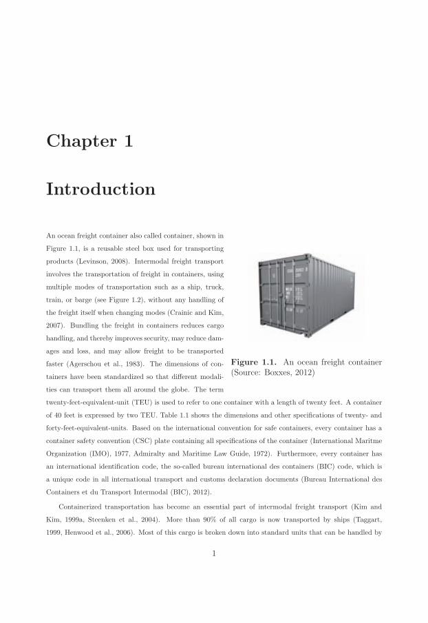
Figure 1.1. An ocean freight container(Source: Boxxes, 2012)
An ocean freight container also called container, shown in
Figure 1.1, is a reusable steel box used for transporting
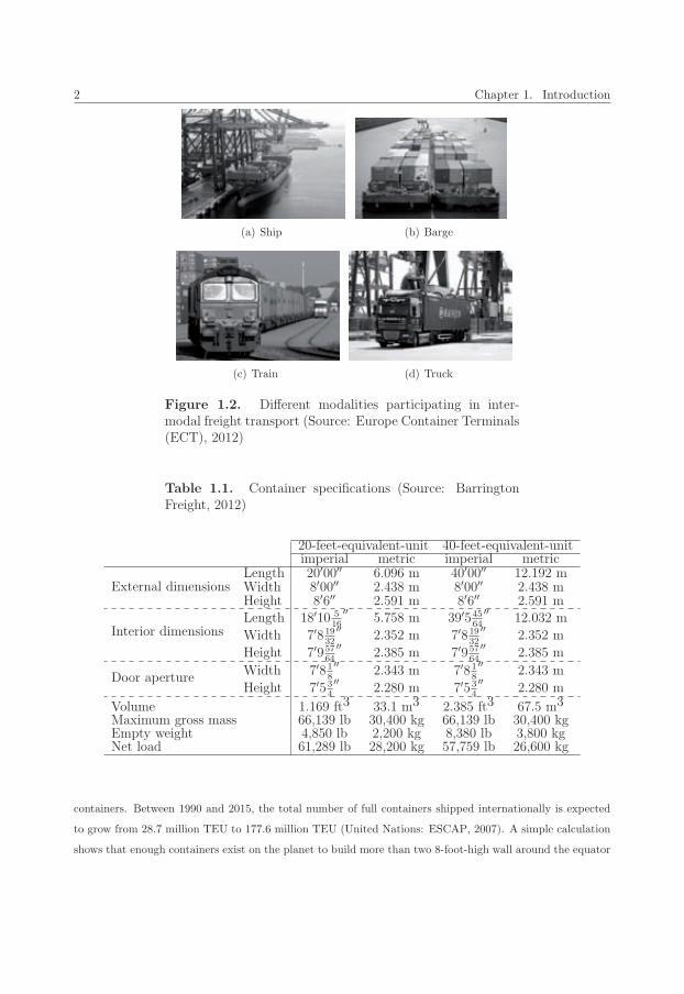
products (Levinson, 2008). Intermodal freight transport
involves the transportation of freight in containers, using
multiple modes of transportation such as a ship, truck,
train, or barge (see Figure 1.2), without any handling of
the freight itself when changing modes (Crainic and Kim,
2007). Bundling the freight in containers reduces cargo
handling, and thereby improves security, may reduce dam-
ages and loss, and may allow freight to be transported
faster (Agerschou et al., 1983). The dimensions of con-
tainers have been standardized so that different modali-
ties can transport them all around the globe. The term
twenty-feet-equivalent-unit (TEU) is used to refer to one container with a length of twenty feet. A container
of 40 feet is expressed by two TEU. Table 1.1 shows the dimensions and other specifications of twenty- and
forty-feet-equivalent-units. Based on the international convention for safe containers, every container has a
container safety convention (CSC) plate containing all specifications of the container (International Maritme
Organization (IMO), 1977, Admiralty and Maritime Law Guide, 1972). Furthermore, every container has
an international identification code, the so-called bureau international des containers (BIC) code, which is
a unique code in all international transport and customs declaration documents (Bureau International des
Containers et du Transport Intermodal (BIC), 2012).
Containerized transportation has become an essential part of intermodal freight transport (Kim and
Kim, 1999a, Steenken et al., 2004). More than 90% of all cargo is now transported by ships (Taggart,
1999, Henwood et al., 2006). Most of this cargo is broken down into standard units that can be handled by
1
2 Chapter 1. Introduction
(a) Ship (b) Barge
(c) Train (d) Truck
Figure 1.2. Different modalities participating in inter-modal freight transport (Source: Europe Container Terminals(ECT), 2012)
Table 1.1. Container specifications (Source: BarringtonFreight, 2012)
20-feet-equivalent-unit 40-feet-equivalent-unitimperial metric imperial metric
External dimensionsLength 20′00′′ 6.096 m 40′00′′ 12.192 mWidth 8′00′′ 2.438 m 8′00′′ 2.438 mHeight 8′6′′ 2.591 m 8′6′′ 2.591 m
Interior dimensionsLength 18′10 5
16
′′5.758 m 39′545
64
′′12.032 m
Width 7′81932
′′2.352 m 7′819
32
′′2.352 m
Height 7′95764
′′2.385 m 7′957
64
′′2.385 m
Door apertureWidth 7′81
8
′′2.343 m 7′81
8
′′2.343 m
Height 7′534
′′2.280 m 7′53
4
′′2.280 m
Volume 1.169 ft3 33.1 m3 2.385 ft3 67.5 m3
Maximum gross mass 66,139 lb 30,400 kg 66,139 lb 30,400 kgEmpty weight 4,850 lb 2,200 kg 8,380 lb 3,800 kgNet load 61,289 lb 28,200 kg 57,759 lb 26,600 kg
containers. Between 1990 and 2015, the total number of full containers shipped internationally is expected
to grow from 28.7 million TEU to 177.6 million TEU (United Nations: ESCAP, 2007). A simple calculation
shows that enough containers exist on the planet to build more than two 8-foot-high wall around the equator
3
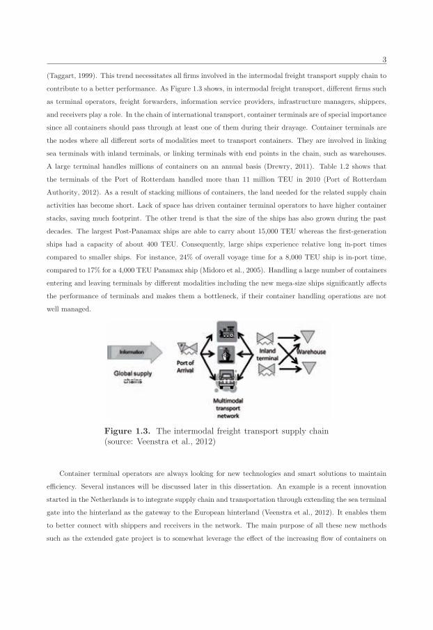
(Taggart, 1999). This trend necessitates all firms involved in the intermodal freight transport supply chain to
contribute to a better performance. As Figure 1.3 shows, in intermodal freight transport, different firms such
as terminal operators, freight forwarders, information service providers, infrastructure managers, shippers,
and receivers play a role. In the chain of international transport, container terminals are of special importance
since all containers should pass through at least one of them during their drayage. Container terminals are
the nodes where all different sorts of modalities meet to transport containers. They are involved in linking
sea terminals with inland terminals, or linking terminals with end points in the chain, such as warehouses.
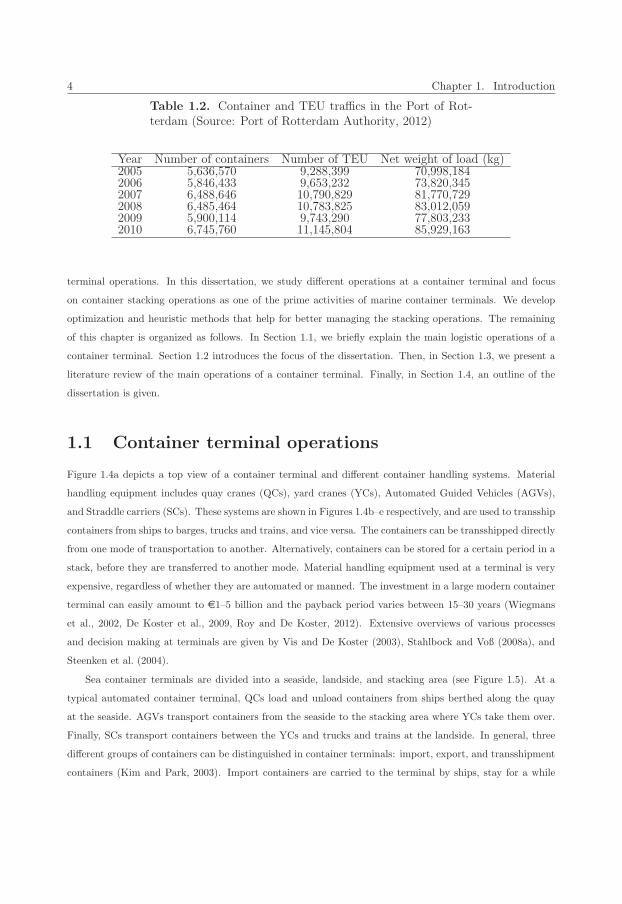
A large terminal handles millions of containers on an annual basis (Drewry, 2011). Table 1.2 shows that
the terminals of the Port of Rotterdam handled more than 11 million TEU in 2010 (Port of Rotterdam
Authority, 2012). As a result of stacking millions of containers, the land needed for the related supply chain
activities has become short. Lack of space has driven container terminal operators to have higher container
stacks, saving much footprint. The other trend is that the size of the ships has also grown during the past
decades. The largest Post-Panamax ships are able to carry about 15,000 TEU whereas the first-generation
ships had a capacity of about 400 TEU. Consequently, large ships experience relative long in-port times
compared to smaller ships. For instance, 24% of overall voyage time for a 8,000 TEU ship is in-port time,
compared to 17% for a 4,000 TEU Panamax ship (Midoro et al., 2005). Handling a large number of containers
entering and leaving terminals by different modalities including the new mega-size ships significantly affects
the performance of terminals and makes them a bottleneck, if their container handling operations are not
well managed.
Figure 1.3. The intermodal freight transport supply chain(source: Veenstra et al., 2012)
Container terminal operators are always looking for new technologies and smart solutions to maintain
efficiency. Several instances will be discussed later in this dissertation. An example is a recent innovation
started in the Netherlands is to integrate supply chain and transportation through extending the sea terminal
gate into the hinterland as the gateway to the European hinterland (Veenstra et al., 2012). It enables them
to better connect with shippers and receivers in the network. The main purpose of all these new methods
such as the extended gate project is to somewhat leverage the effect of the increasing flow of containers on
4 Chapter 1. Introduction
Table 1.2. Container and TEU traffics in the Port of Rot-terdam (Source: Port of Rotterdam Authority, 2012)
Year Number of containers Number of TEU Net weight of load (kg)2005 5,636,570 9,288,399 70,998,1842006 5,846,433 9,653,232 73,820,3452007 6,488,646 10,790,829 81,770,7292008 6,485,464 10,783,825 83,012,0592009 5,900,114 9,743,290 77,803,2332010 6,745,760 11,145,804 85,929,163
terminal operations. In this dissertation, we study different operations at a container terminal and focus
on container stacking operations as one of the prime activities of marine container terminals. We develop
optimization and heuristic methods that help for better managing the stacking operations. The remaining
of this chapter is organized as follows. In Section 1.1, we briefly explain the main logistic operations of a
container terminal. Section 1.2 introduces the focus of the dissertation. Then, in Section 1.3, we present a
literature review of the main operations of a container terminal. Finally, in Section 1.4, an outline of the
dissertation is given.
1.1 Container terminal operations
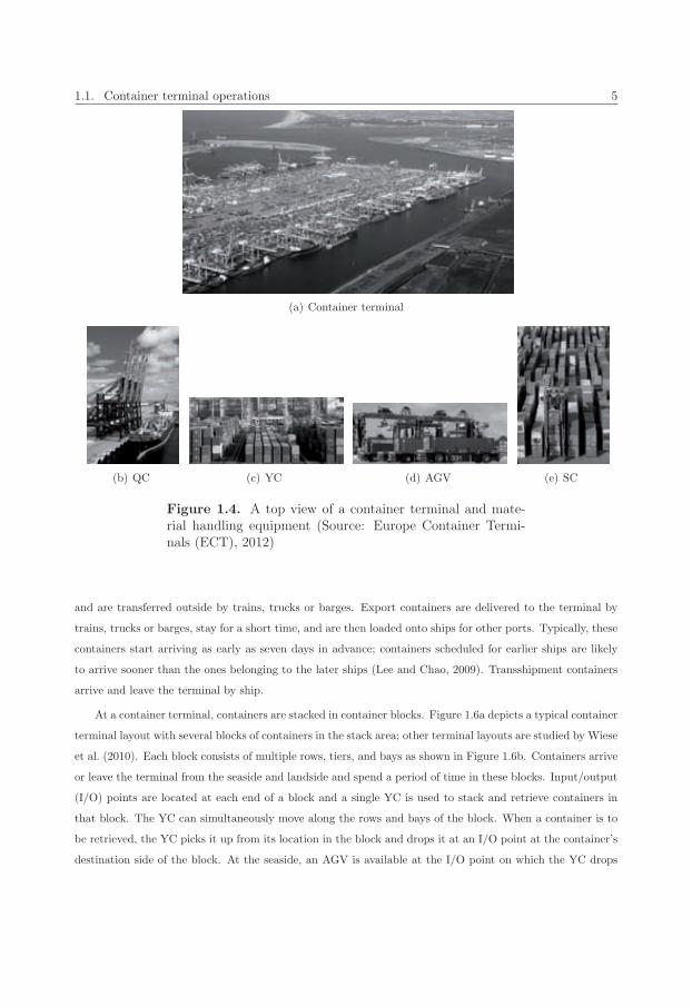
Figure 1.4a depicts a top view of a container terminal and different container handling systems. Material
handling equipment includes quay cranes (QCs), yard cranes (YCs), Automated Guided Vehicles (AGVs),
and Straddle carriers (SCs). These systems are shown in Figures 1.4b–e respectively, and are used to transship
containers from ships to barges, trucks and trains, and vice versa. The containers can be transshipped directly
from one mode of transportation to another. Alternatively, containers can be stored for a certain period in a
stack, before they are transferred to another mode. Material handling equipment used at a terminal is very
expensive, regardless of whether they are automated or manned. The investment in a large modern container
terminal can easily amount to e1–5 billion and the payback period varies between 15–30 years (Wiegmans
et al., 2002, De Koster et al., 2009, Roy and De Koster, 2012). Extensive overviews of various processes
and decision making at terminals are given by Vis and De Koster (2003), Stahlbock and Voß (2008a), and
Steenken et al. (2004).
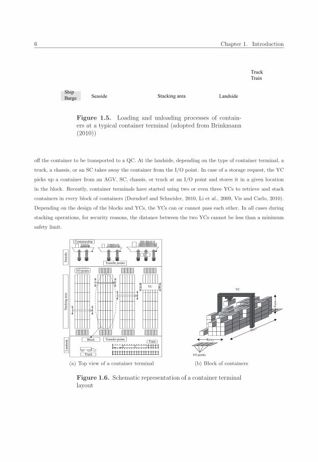
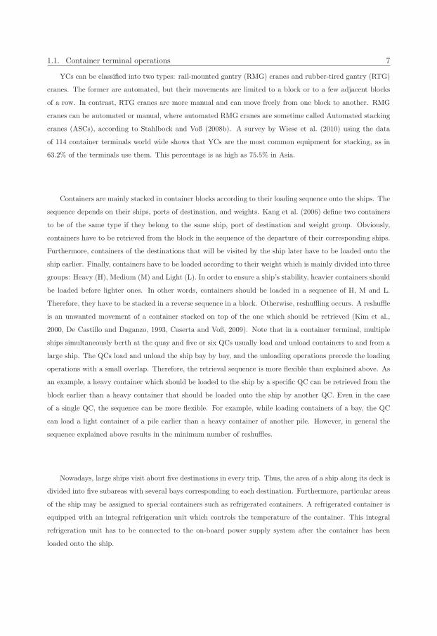
Sea container terminals are divided into a seaside, landside, and stacking area (see Figure 1.5). At a
typical automated container terminal, QCs load and unload containers from ships berthed along the quay
at the seaside. AGVs transport containers from the seaside to the stacking area where YCs take them over.
Finally, SCs transport containers between the YCs and trucks and trains at the landside. In general, three
different groups of containers can be distinguished in container terminals: import, export, and transshipment
containers (Kim and Park, 2003). Import containers are carried to the terminal by ships, stay for a while
1.1. Container terminal operations 5
(a) Container terminal
(b) QC (c) YC (d) AGV (e) SC
Figure 1.4. A top view of a container terminal and mate-rial handling equipment (Source: Europe Container Termi-nals (ECT), 2012)
and are transferred outside by trains, trucks or barges. Export containers are delivered to the terminal by
trains, trucks or barges, stay for a short time, and are then loaded onto ships for other ports. Typically, these
containers start arriving as early as seven days in advance; containers scheduled for earlier ships are likely
to arrive sooner than the ones belonging to the later ships (Lee and Chao, 2009). Transshipment containers
arrive and leave the terminal by ship.
At a container terminal, containers are stacked in container blocks. Figure 1.6a depicts a typical container
terminal layout with several blocks of containers in the stack area; other terminal layouts are studied by Wiese
et al. (2010). Each block consists of multiple rows, tiers, and bays as shown in Figure 1.6b. Containers arrive
or leave the terminal from the seaside and landside and spend a period of time in these blocks. Input/output
(I/O) points are located at each end of a block and a single YC is used to stack and retrieve containers in
that block. The YC can simultaneously move along the rows and bays of the block. When a container is to
be retrieved, the YC picks it up from its location in the block and drops it at an I/O point at the container’s
destination side of the block. At the seaside, an AGV is available at the I/O point on which the YC drops
6 Chapter 1. Introduction
Figure 1.5. Loading and unloading processes of contain-ers at a typical container terminal (adopted from Brinkmann(2010))
off the container to be transported to a QC. At the landside, depending on the type of container terminal, a
truck, a chassis, or an SC takes away the container from the I/O point. In case of a storage request, the YC
picks up a container from an AGV, SC, chassis, or truck at an I/O point and stores it in a given location
in the block. Recently, container terminals have started using two or even three YCs to retrieve and stack
containers in every block of containers (Dorndorf and Schneider, 2010, Li et al., 2009, Vis and Carlo, 2010).
Depending on the design of the blocks and YCs, the YCs can or cannot pass each other. In all cases during
stacking operations, for security reasons, the distance between the two YCs cannot be less than a minimum
safety limit.
(a) Top view of a container terminal (b) Block of containers
Figure 1.6. Schematic representation of a container terminallayout
1.1. Container terminal operations 7
YCs can be classified into two types: rail-mounted gantry (RMG) cranes and rubber-tired gantry (RTG)
cranes. The former are automated, but their movements are limited to a block or to a few adjacent blocks
of a row. In contrast, RTG cranes are more manual and can move freely from one block to another. RMG
cranes can be automated or manual, where automated RMG cranes are sometime called Automated stacking
cranes (ASCs), according to Stahlbock and Voß (2008b). A survey by Wiese et al. (2010) using the data
of 114 container terminals world wide shows that YCs are the most common equipment for stacking, as in
63.2% of the terminals use them. This percentage is as high as 75.5% in Asia.
Containers are mainly stacked in container blocks according to their loading sequence onto the ships. The
sequence depends on their ships, ports of destination, and weights. Kang et al. (2006) define two containers
to be of the same type if they belong to the same ship, port of destination and weight group. Obviously,
containers have to be retrieved from the block in the sequence of the departure of their corresponding ships.
Furthermore, containers of the destinations that will be visited by the ship later have to be loaded onto the
ship earlier. Finally, containers have to be loaded according to their weight which is mainly divided into three
groups: Heavy (H), Medium (M) and Light (L). In order to ensure a ship’s stability, heavier containers should
be loaded before lighter ones. In other words, containers should be loaded in a sequence of H, M and L.
Therefore, they have to be stacked in a reverse sequence in a block. Otherwise, reshuffling occurs. A reshuffle
is an unwanted movement of a container stacked on top of the one which should be retrieved (Kim et al.,
2000, De Castillo and Daganzo, 1993, Caserta and Voß, 2009). Note that in a container terminal, multiple
ships simultaneously berth at the quay and five or six QCs usually load and unload containers to and from a
large ship. The QCs load and unload the ship bay by bay, and the unloading operations precede the loading
operations with a small overlap. Therefore, the retrieval sequence is more flexible than explained above. As
an example, a heavy container which should be loaded to the ship by a specific QC can be retrieved from the
block earlier than a heavy container that should be loaded onto the ship by another QC. Even in the case
of a single QC, the sequence can be more flexible. For example, while loading containers of a bay, the QC
can load a light container of a pile earlier than a heavy container of another pile. However, in general the
sequence explained above results in the minimum number of reshuffles.
Nowadays, large ships visit about five destinations in every trip. Thus, the area of a ship along its deck is
divided into five subareas with several bays corresponding to each destination. Furthermore, particular areas
of the ship may be assigned to special containers such as refrigerated containers. A refrigerated container is
equipped with an integral refrigeration unit which controls the temperature of the container. This integral
refrigeration unit has to be connected to the on-board power supply system after the container has been
loaded onto the ship.
8 Chapter 1. Introduction
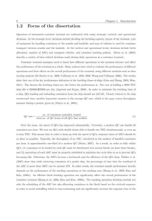
1.2 Focus of the dissertation
Operators of automated container terminal are confronted with many strategic, tactical, and operational
decisions. At the strategic level, decisions include deciding the berthing capacity, layout of the terminal, type
of equipment for handling containers at the seaside and landside, and type of vehicles to used for container
transport between seaside and the landside. At the tactical and operational levels, decisions include berth
allocation, number of ASCs and transport vehicles, and container stacking policies. Murty et al. (2005)
describe a variety of inter-related decisions made during daily operations at a container terminal.
Container terminal managers need to know how different operations at the terminal interact and affect
the performance of the terminal as a whole. Many authors have tried to evaluate the performance of different
operations and their effects on the overall performance of the terminal, using different methods such as data
envelop analysis (De Koster et al., 2009, Cullinane et al., 2005, 2006, Wang and Cullinane, 2006). The results
show that one of the key performance indicators is the berthing times of ships (Linn and Zhang, 2003, Bose,
2011). The shorter the berthing times are, the better the performance is. The cost of holding a 2000 TEU
ship idle is �20000-�25000 per day (Agarwal and Ergun, 2008). In order to minimize the berthing time of
a ship, QCs loading and unloading containers from the ship should not fall idle. Closely related to the ship
turnaround time, another important measure is the average QC rate, which is the quay cranes throughput
measure during a period, given by (Murty et al., 2005):
QC rate =no. of containers unloaded, loaded
total no. of QC hours of all QCs that worked(1)
Over the years, the speed of QCs has improved substantially. Currently, a modern QC can handle 35
containers per hour. We now see QCs with double hoists able to handle two TEU simultaneously, or even up
to four TEU. This means that in order to keep up with the speed of QCs, response times of ASCs should be
as short as possible. Typically, the throughput of an ASC, calculated as the number of handled containers
per hour, is approximately one-third of a modern QC (Murty, 2007). As a result, in order to fully utilize
QCs, (1) containers to be loaded by each QC must be distributed over several blocks (at least three blocks),
and (2) operations of each ASC must be properly scheduled to minimize the cycle time so as to prevent QCs
becoming idle. Otherwise, the ASCs become a bottleneck and the efficiency of the QCs drop. Dekker et al.
(2007) show that while retrieving containers of a jumbo ship, the percentage of time that the workload of
the ASC is more than 100% can be around 10%. In other words, the terminal seaside performance heavily
depends on the performance of the stacking operations at the stacking area (Zhang et al., 2002, Kim and
Kim, 1999a). An efficient block stacking operation can significantly affect the overall performance of the
container terminal (Zhang et al., 2002, Kim and Kim, 1999a). The stacking operation decisions include not
only the scheduling of the ASC but also allocating containers in the block based on the retrieval sequence
in order to avoid reshuffling which is time-consuming and can significantly increase the response time of the
1.3. Literature review 9
ASC.
The importance of stacking operation decisions becomes more clear considering the fact that while re-
trieving containers for a ship, each ASC also should retrieve containers leaving the terminal by truck and train
at the landside. In addition, it should stack containers arriving at the I/O points of the block by AGVs from
the seaside or by trucks and trains from the landside. Stacking operations of the ASC should be optimized to
prevent it from becoming a bottleneck. Otherwise, not only the berthing time of the ship may significantly
increase but also the waiting times of trucks, and trains. It is therefore important to minimize the makespan
of all requests to be performed by the ASC by optimally sequencing them. In practice, usually simple ASC
scheduling rules are deployed, such as nearest neighbor (NN) or first-come-first-served (FCFS). In the NN
heuristic, the ASC carries out the nearest container, and in the FCFS heuristic, it carries out the containers
based on their arrival sequence. A more proper schedule might considerably reduce the total travel time of
the ASC, which consequently reduces the makespan of ships and waiting times of trucks, barges, and trains.
In case of a container terminal with multiple rows and a straddle carrier to store and retrieve containers, Vis
and Roodbergen (2009) show that the time difference between the optimal and FCFS sequence is at least
30%. Although an ASC operates differently from a straddle carrier, substantial travel time reduction may
be gained for the ASC as well.
This dissertation focuses on the operations at the stacking area of a container terminal. More specifically,
we consider the problem of scheduling ASCs to stack and retrieve containers. We also study where storage
containers have to be stacked not only from the viewpoint of reducing the ASC travel time but also to
minimize the number of reshuffles. In the next section, we review the previous theoretical papers on these
topics, and then in Section 1.4, the outline of the dissertation is explained.
1.3 Literature review
The literature on tactical and operational decision problems at container terminals is dense (see, for example,
Gunther and Kim, 2005, Steenken et al., 2004, Stahlbock and Voß, 2008a). In some research papers, the
interaction between different systems at a container terminal is discussed, whereas in the other papers the
focus is on improving the performance of an individual operation. Simulation is the prime tool to analyze the
integration and interaction of different systems (Petering and Murty, 2009, Petering et al., 2009, Petering,
2011a, 2010, Liu et al., 2002, 2004, Roy and De Koster, 2012). More than 40 papers on simulation models
can be found in the literature which range from strategic to operational decision making (Petering et al.,
2009).
Exact and heuristic methods are more common when it comes to analyzing the individual processes at
a container terminal. For example, routing and dispatching AGVs are studied by Kim and Bae (2004), Vis
et al. (2001), Evers and Koppers (1996), Vis et al. (2005), Briskorn et al. (2006), Lehmann et al. (2006),
and Meersmans (2002). Scheduling SCs is studied by Vis and Roodbergen (2009), Kim and Kim (1999c,b),
10 Chapter 1. Introduction
Kozan and Preston (1999), and Kozan (2000). Scheduling QCs can be found in Daganzo (1989), Kang et al.
(2008), Goodchild and Daganzo (2006), Choo et al. (2010), and Zhen et al. (2011). Some papers focus on the
berth allocation problem. The problem involves the allocation of ships to berth places in time in order to
optimize a certain objective function. In most of the reported studies, the objective is to minimize each ship’s
turnaround time (Hendriks et al., 2010, Kim and Moon, 2003, Guan and Cheung, 2004, Cordeau et al., 2005,
Imai et al., 2005, Monaco and Sammarra, 2007, Moorthy and Teo, 2006). A limited number of studies consider
a multi-objective problem, where besides the turnaround times, the weighted deviations from predetermined
berth positions are minimized (Wang and Lim, 2007, Hansen et al., 2008). Last but not least, scheduling
and routing ships are studied by Agarwal and Ergun (2008), Christiansen et al. (2004), Sherali et al. (1999),
Brown et al. (1987), Appelgren (1969, 1971), Ronen (1983) and Ronen (1993).
Since this dissertation focuses on the ASC scheduling and the container reshuffling problem, we particulary
pay attention to these two sections of the literature in the following subsections. Surprisingly, in spite of the
importance of these issues for daily terminal operations, relatively little research attention has been given to
these topics.
1.3.1 Yard crane scheduling
ASC, or yard crane (YC) scheduling, has not been studied well. Most of the relevant papers do not specify
any special type of YC (i.e. manual or automated RMG or RTG crane) and as such the models and solution
methods developed are applicable to all sorts of YC. However, the assumptions considered often show that
the models are more suitable for a special type of crane and must be tweaked in different ways in order to
be used to schedule another type of crane. All in all, since most papers do not specifically mention the type
of crane, we use the general term “yard crane (YC)” to review the literature.
Kim and Kim (1999a) schedule a YC to retrieve containers from several blocks in the stacking area of a
terminal. They propose a discrete time network model in which the objective is to minimize the total travel
time of the crane to carry out all retrieval requests. Narasimhan and Palekar (2002) also study a model in
which a single YC retrieves containers from a single block. Containers are classified into several types and
while retrieving a container of a specific type, the ASC selects one of the containers of that type available in
different locations of the block. They prove that the problem is NP-hard and develop a branch-and-bound
algorithm. For large size instances, they propose a heuristic with a worst-case performance ratio of 1.5. Ng
(2005) schedules several YCs to carry out a set of retrieval requests with different ready times in a yard zone,
defined as multiple blocks located behind each other in a row. The YCs cannot pass each other and cannot
exit the zone. They propose a discrete time mixed integer model and solve it by means of a heuristic based
on dynamic programming. The objective function is to minimize the total completion time. Ng and Mak
(2005) have later proposed an exact branch-and-bound algorithm for the same problem, but with a single
crane. The objective function is to minimize the total waiting time of all requests.
In more recent papers, retrieval and storage requests are considered simultaneously. Zhang et al. (2002)
1.3. Literature review 11
propose a discrete time mixed integer linear model for a problem in which several YCs carry out a given
workload in multiple blocks. Based on their definition, a workload can consist of storage and retrieval requests.
The objective is to minimize the total unfinished workload at the end of each time period. They propose
a Lagrangian relaxation model and a heuristic method to solve the problem. Cheung et al. (2002) study a
similar problem and prove that it is NP-hard in the strong sense. In order to solve the problem, they propose
a Lagrangian relaxation exact algorithm, as well as an approximation method which formulates the problem
as a network flow model with a piecewise-linear objective function.
Since the use of twin cranes limited to a block of containers is a new technology, scheduling models for such
configurations can only be found in more recent papers. Li et al. (2009) introduce a discrete time model to
schedule two ASCs carrying out the storage and retrieval requests in a single block with an I/O point located
at one side of the block along the bays. The ASCs cannot pass each other and must be separated by a safety
distance. The requests have different due times and the objective is to minimize a weighted combination of
earliness and lateness of all requests, compared to their due times. They introduce a rolling horizon algorithm
in which a horizon of a specific length is defined, and all requests falling within this horizon are considered
and optimized by CPLEX. The horizon is updated whenever all its requests have been scheduled. Vis and
Carlo (2010) also consider a similar setting. However, in their problem the ASCs can pass each other but
cannot work on the same bay simultaneously. In their problem, requests do not have any due time and can
be scheduled in any sequence. They formulate the problem as a continuous time model and minimize the
makespan of the ASCs. They solve it by a simulated annealing algorithm and use the single-row method
proposed by Vis (2006) to compute a lower bound.
Note that some papers focus on scheduling SCs (Vis and Roodbergen, 2009, Hartmann, 2004, Steenken
et al., 1993, Kim and Kim, 1999c,b). An SC can only operate on a single row of containers, where containers
of that row pass a landside or seaside I/O point located at the end of it depending on the side of destination.
Since traveling from one row to another one is time-consuming, the SC completes all requests associated
with a given row consecutively. Based on this property of the problem, Vis and Roodbergen (2009) first
use dynamic programming to route the SC among the rows of containers and then use a single-row-method
proposed by Vis (2006) to optimally route the SC in each row in a polynomial time.
Finally, in order to increase the performance of a container terminal, YCs and QCs not only must be
scheduled optimally but also must be synchronized with AGVs. In this regard, some authors deal with
optimizing the number of AGVs or synchronizing them with other material handling equipment at the
terminal (Vis et al., 2001, 2005, Bish et al., 2005, Kim and Bae, 2004, Li and Vairaktarakis, 2004, Roy and
De Koster, 2012).
1.3.2 Minimizing container reshuffling
Papers dealing with container reshuffling study three main subjects: (1) estimating the number of reshuffles,
(2) pre-marshalling, and (3) stacking methods to reduce the number of reshuffles. As it will be discussed
12 Chapter 1. Introduction
later in this section, due to the complexity of the models concerning these issues, many focus on only a single
bay with few piles for stacking or pre-marshalling containers (Froyland et al., 2008). In order to solve a
single-bay problem, some authors try to increase the quality and speed of their algorithms by local search
methods (Caserta and Voß, 2009, Lee and Chao, 2009). As a result, the need for studying a holistic problem
which considers a whole block of containers exists.
In order to estimate the expected number of reshuffles which results from a given number of storage
handlings, Kang et al. (2006) use simulated annealing assuming that containers belong to a single ship. Based
on this, they introduce a probabilistic formula to estimate the total expected number of reshuffles. Kim (1997)
proposes a method based on dynamic programming in combination with two heuristic algorithms to estimate
the total number of reshuffles. In a recent paper, Lee and Kim (2010) employ this estimation in a model to
optimize the block size taking into consideration the required throughput of YCs. De Castillo and Daganzo
(1993) also develop general expressions to calculate the expected number of reshuffles to retrieve a container
under segregation and non-segregation stacking strategies. Under the segregation strategy, containers are
separated based on their duration of stay. They assume no new container will be stacked.
Some researchers focus on how to reduce the number of reshuffles by pre-marshaling containers in a way
that fits the ships’ stowage plans. Pre-marshaling is the repositioning of containers of the block prior to the
ship arrival so that no or few reshuffles are needed when containers are loaded onto the ships. Lee and Hsu
(2007) propose an integer programming model for a container pre-marshaling problem preventing reshuffling.
They develop a multi-commodity network flow model for obtaining a plan on how to pre-marshal containers
stacked in some piles of containers. They also propose a simple heuristic for large-scale problems. Lee and
Chao (2009) develop a neighborhood-based heuristic model to pre-marshal containers of a single bay in order
to find a desirable final bay plan. Caserta and Voß (2009) also study a similar container pre-marshaling
problem. They propose a dynamic programming model to pre-marshal containers of a single bay. In order to
quickly find the solution, they propose a corridor method. In this local search method, when a container is
being pre-marshaled it can only be stacked in a corridor which consist of the next few predecessor or successor
piles of the bay with a specific limit on the number of empty locations.
Some papers focus on how to avoid reshuffling by proposing methods to properly locate incoming con-
tainers in a container block. Dekker et al. (2007) investigate different stacking policies, using simulation
based on real data. They allocate the containers to the block based on the containers’ expected duration
of stay. Kim and Park (2003) also propose a heuristic algorithm based on the containers’ duration of stay
to locate containers. Kim et al. (2000) propose a stochastic dynamic programming model for determining
storage positions of export containers in a single bay of a block. To avoid solving a time-consuming dynamic
programming model for each incoming container, they build decision trees, using the optimal solutions of
the dynamic programming model. The trees tell where to store an incoming container. The validity of the
recursive function of the dynamic programming model is proven by Zhang et al. (2010).
1.4. Outline of the dissertation 13
1.4 Outline of the dissertation
Motivated by the discussions in section 1.2 and the literature in section 1.3, this dissertation proposes,
develops, and tests optimization methods to support the decisions of container terminal operators in the
stacking area of a terminal. We focus on operational stacking problems, which are treated in four chapters.
The first three chapters focus on sequencing a given set of container storage and retrieval requests in a single
block. All three problems are complex and modeled as continuous time integer programming models. The
objective is to minimize the makespan to carry out all requests. As discussed in section 1.2, we can improve
the performance of the terminal by minimizing the makespan. We try to optimally solve the problems as long
as the complexity allows it. Otherwise, heuristic algorithms are developed to obtain near-optimal solutions.
The last chapter links indirectly to the first three and will be discussed later. Although some theoretical
studies have already addressed parts of the problems considered in this dissertation, our specific models
incorporating the constraints that are faced in practice have, to the best of our knowledge, not yet been
addressed in literature.
In Chapter 2, we minimize the travel time of a single ASC to carry out all requests. The ASC must move
retrieval containers from the block to the I/O points, and must move storage containers from the I/O points
to the block. Locations as well as destination sides of retrieval containers and I/O points of storage containers
are known. The problem is formulated as an asymmetric traveling salesman problem (ATSP). The objective
is to minimize the total travel time of the ASC to perform all requests. Different than the literature discussed
above, we optimally solve the ATSP model for instances of all sizes. In most of the previous research papers,
discrete time models are proposed and mainly heuristics are used to solve the models.
In Chapter 3, we consider a similar problem with the difference that storage locations are not given. In
other words, in case of a storage request, the ASC picks up a container from an I/O point, and drops it
off in a location selected from a set of open locations suitable for stacking the container. Since container
terminal operators often separate containers based on several criteria such as destination and weight, a set
of open suitable locations is in many cases available to stack the container. We formulate the problem as a
generalized asymmetric traveling salesman problem (GATSP). Similar to the previous problem, we minimize
the total travel time of the ASC to perform all requests. In this problem, a single location may be suitable
for stacking different containers, and thus sets of open locations may overlap. Locations in the intersection
of multiple sets make the problem complex. Extra constraints are necessary to stack at most one container
in such a location. In the literature, no continuous time model for such problem is proposed. We formulate
the problem and solve it for small and medium instances. For large instances, we use a heuristic algorithm
to obtain near-optimal solutions.
Chapter 4 considers a problem in which two ASCs carry out the requests. The ASCs can never pass each
other and must operate sufficiently far from each other. Furthermore, the storage locations are not given and,
in addition, containers can have different priorities in order to be stacked or retrieved. The most important
reasons for this are as follows:
14 Chapter 1. Introduction
� The performance of a container terminal is often evaluated based on the berthing times of ships (Bose,
2011). Therefore, seaside containers usually have a higher priority than landside containers.
� To ensure the stability of ships, heavy containers must be loaded before light containers, in lower tiers
on the ship and must therefore be retrieved earlier (see, for example, Gharehgozli et al., 2012c, Kim
et al., 2000, Sammarra et al., 2007, Dekker et al., 2007).
� Trucks, trains and ships arrive at a container terminal to deliver or pick up containers at different
points in time (see, for example, Froyland et al., 2008, Petering, 2011b, Newman and Yano, 2000),
which induces precedence constraints on the stacking and retrieving of containers.
Preventing reshuffling also imposes additional precedence constraints on the operations. A precedence
constraint can prohibit a container to be stacked in a pile before retrieving a container located in the same
pile, or it can force containers stacked on top of a specific container to be retrieved earlier.
We formulate this multi-crane problem as a multiple asymmetric generalized traveling salesman problem
with precedence constraints (mAGTSP-PC), which generalizes the single version of the problem without such
constraints (see, for example, Laporte et al., 1987, Noon and Bean, 1991). The objective is to minimize the
makespan of the two ASCs. The model also contains additional constraints regarding the interactions of
the ASCs and the selection of open storage locations which lie in the intersection of multiple sets. Stacking
problems with two ASCs have hardly researched. The combination with precedence constraints, and multiple
open locations for storage containers is new. The new extra constraints make the problem so complex that
we develop an adaptive large neighborhood search heuristic to solve the problem.
In these chapters, the storage locations can be selected from sets of open locations. However, it is assumed
that these locations are still determined beforehand at a higher level in the decision making hierarchy. Chapter
5 is an attempt to find proper locations among all available empty locations when containers arrive at the
container terminal. The objective function is to minimize the expected number of reshuffles.
Chapter 2
Scheduling a Single Yard Crane with
Given Storage Locations∗
Container terminals play a vital role in the organization of efficient global trade (Taggart, 1999, Henwood
et al., 2006). A large terminal handles millions of containers annually, which are transported by deep-sea
vessels of increasingly larger sizes (Drewry, 2011). Containers arriving at a terminal are stored in a very large
yard until they can be loaded onto proper outbound transport modes, like other deep-sea ships, barges, trains
or trucks. At a terminal, containers are stacked in container blocks, each operated by a single automated
stacking crane (ASC) (see Chapter 1). The stack decouples flows between different transport modes, like
deepsea and shortsea vessels, barges, trains, and trucks, in time. Particulary for large vessels, it is known some
time in advance which containers have to be unloaded and loaded, to and from which position in the stack.
Modes with smaller drop sizes, such as barges and trucks have to be scheduled in between the large-scale
operations of deep-sea vessels. Minimizing the makespan of deep-sea vessels is a prime overall objective at a
container terminal. However, the ASc has to handle requests for other modes as well within the given time
frame. Since the ASC is often a heavily utilized resource at a container terminal, it is necessary to schedule
the stacking operations over a given horizon with throughput time minimization as a prime objective (Bose,
2011). In practice, storage and retrieval requests are often executed in a first-come-first-served (FCFS) order
or by the nearest neighbor (NN) search, as provided by commercial software companies (for example, Cosmos
NV and Modality Software solutions b.v.). A more proper schedule can considerably reduce the total travel
time of the ASC, which consequently reduces the makespan of ships and waiting times of trucks, barges, and
trains.
We consider the problem of sequencing a given set of requests to be stacked or retrieved by an ASC in a
single block. The objective is to minimize the travel time of the ASC to carry out the requests. We formulate
∗This chapter is based on Gharehgozli et al. (2012d).
15
16 Chapter 2. Scheduling a Single Yard Crane with Given Storage Locations
this problem with multiple I/O points as a special kind of an asymmetric traveling salesman problem (ATSP),
in which to travel between two request locations in the block, the ASC, in most cases, must visit an I/O
point. We show that due to the existence of multiple I/O points and the special movements of the ASC,
the problem is so complex and in a special case is NP-hard. For quickly solving the problem, we propose a
two-phase solution method. In the first phase of the solution, we develop a new merging algorithm to patch
subtours of an optimal solution of the assignment problem (AP) relaxation of the problem without adding
extra travel time. In this phase, we first search for two arcs from every two different subtours visiting a
common I/O point, and swap the destinations of them to merge the subtours. Next, based on the fact that in
some arcs, the ASC has multiple I/O point options with the same travel time to visit, we can create further
opportunities to merge more subtours. We show that the first phase runs in a polynomial time, and often
finds an optimal solution. Otherwise, a branch-and-bound (B&B) algorithm is used in the second phase to
find an optimal solution of the problem. In this phase, the merging algorithm is again used in each node of
the B&B tree to save computation time.
The numerical results show the two-phase solution method is quite efficient. For instances up to 200
requests, an optimal solution can be obtained in less than a second. Furthermore, we show that the travel
time reduction between the optimal and FCFS sequence is around 30%, on average. The reduction is around
14%, in case the NN heuristic is used to find the sequence. Finally, in order to evaluate the complexity of
the problem and the performance of our algorithm, we compare our results with CPLEX results. The results
show that the two-phase solution method can obtain significantly better results than CPLEX truncated after
five hours. For instances with 100 requests, CPLEX cannot obtain a feasible solution after five hours.
In general, scheduling a yard crane to carry out storage and retrieval requests can be modeled as an
ATSP or one of its special cases such as the rural postman problem, or Chinese postman problem, depending
on the properties of the problem (Vis and Roodbergen, 2009). Simply stated, the ATSP is a combinatorial
problem in which from a given list of locations with given pairwise travel times, a tour must be determined
passing every location exactly once in such a way that the total travel time is minimized (Lawler et al.,
1985). In general, ATSP is proved to be NP-hard (see, for example, Srour and Van de Velde, 2011). Several
algorithms have been proposed to solve the ATSP. Among the most efficient ones is the B&B algorithm
based on the subtour elimination approach proposed by Carpaneto and Toth (1980) and later improved by
Carpaneto et al. (1995) and Miller and Pekny (1991). The core idea of the B&B algorithm in all three studies
is the AP relaxation. In each node of the B&B tree, an AP with some extra constraints is solved. Constraints
exclude a number of arcs and require some others to appear in the AP solution so that some subtours can be
avoided. Carpaneto et al. (1995) and Miller and Pekny (1991) also propose two merging algorithms. In these
algorithms, the reduced costs of the arcs are used to merge subtours, and they are thus time consuming.
Therefore, Carpaneto et al. (1995) for example use the merging algorithm in every node if the number of
zero-reduced cost arcs is more than a threshold. In addition, the objective value may increase after merging
subtours. These issues make their algorithms different than the one developed in this chapter, in a sense that
17
our algorithm uses swappable arcs with common visiting I/O points to quickly patch subtours without extra
travel time.
Reviewing the papers on scheduling a single crane to carry out storage and retrieval requests of containers
at a container terminal (Vis and Roodbergen, 2009) or of unit loads in a warehouse (Ratliff and Rosenthal,
1983, De Koster and Van der Poort, 1998, Van den Berg and Gademann, 1999) reveals that specific properties
of each individual problem, modeled as a form of ATSP, determine whether a polynomial solution method
can be developed. These properties are: (1) the number of I/O points, and (2) the number of rows in which
containers are stored or retrieved. The literature can therefore be categorized based on these properties as
follows.
In case of a single I/O points, polynomial solution methods can be developed (see Burkard et al. (1998)
for solvable TSP cases). In this case, all subtours of an optimal solution of an AP relaxation to the ATSP
can be merged as a complete Hamiltonian tour, since the crane returns to the same I/O point for every
request. Having returned to the I/O point, the crane can select any storage request. It can also select a
retrieval request in case in the optimal AP solution that retrieval request is sequenced after another retrieval
request. Therefore, all subtours can be merged without adding extra travel time. Nevertheless, by increasing
the number of I/O points, the problem becomes more complex. In fact, we show that the general problem
with multiple I/O points is NP-hard.Van den Berg and Gademann (1999) discuss a problem with both an output point and an input point,
which is a special case of a problem with a single I/O point. As a result, although locations are spread in
multiple rows, an optimal solution can efficiently be found. They formulate the problem as a transportation
problem using a bipartite graph and prove that each feasible solution of the transportation problem corre-
sponds to a retrieval and storage sequence of the main problem. Note that they assume storage requests are
executed in a FCFS order. The problem is to find which retrieval requests must be interleaved after each
storage.
Vis and Roodbergen (2009) consider a problem with a single block where the block corresponds to
multiple rows separated by aisles. Each row has one I/O point at each end which serve that row. A single
straddle carrier stores or retrieves all containers in the rows, where each container passes an appropriate I/O
point of its row. The straddle carrier must exit the current row at the end in order to travel from one row to
the other one, which is time-consuming. Therefore, it usually finishes all requests in that row before traveling
to another. Based on this specific characteristic of straddle carriers, they can decompose the problem with
multiple rows into several problems with one row and two I/O points and solve them separately. They
propose a solution method based on dynamic programming to determine the shortest path for the straddle
carrier crossing multiple rows. The dynamic programming allows multiple visits of a single row. It uses an
optimal storage and retrieval request sequence in each row. Using an optimal AP solution to sequence the
requests in a row with two I/O points results in maximum two subtours. They prove that these subtours
can be optimally merged by enumerating and exchanging arcs in O(N) time because in case of a single row
18 Chapter 2. Scheduling a Single Yard Crane with Given Storage Locations
and two I/O points, because the travel time matrix has the properties of a Monge matrix (see Gilmore and
Gomory, 1964). Vis and Carlo (2010) also use the same method to find a lower bound for their container
sequencing problem with a single block and two ASCs. To obtain the lower bound, they collapse all rows of
the block together as a single row and assume that a single ASC carries out all requests. Considering two
ASCs to carry out the requests makes the problem complex that they resort to a metaheuristic to solve the
problem.
Vis and Roodbergen (2009) extend the models proposed by Ratliff and Rosenthal (1983) and De Koster
and Van der Poort (1998) for routing an orderpicker in a warehouse. Ratliff and Rosenthal (1983) consider
a warehouse with parallel aisles (comparable to a container terminal with parallel rows), a central I/O point
and no storage request, whereas De Koster and Van der Poort (1998) consider the same situation but the
warehouse can have an I/O point at the end of each aisle. Dynamic programming is used in both studies to
decompose and solve the problems.
Different from the previous line of research, in this paper, a continuous time integer programming model
is proposed to stack and retrieve containers in a block with multiple I/O points and rows densely located
together. Since the ASC can simultaneously move across the rows and does not return to the row ends
to switch rows, the problem is more complex. Compared to the current ASC position, many locations in
neighbor rows have identical travel times. In order to obtain the optimal solution, all rows and I/O points
must be considered at the same time in the solution method. Decomposing the block into multiple single-row
blocks for adopting the methods proposed by Vis and Roodbergen (2009), De Koster and Van der Poort
(1998), Ratliff and Rosenthal (1983) is not possible, since returning to an I/O point located at either end
of each row is essential in the proposed network models and solution methods. Extra arcs are necessary
in the network to model switching rows without returning to the I/O points. Even if the block is divided
into multiple single-row blocks, the optimal solution of each row cannot be obtained using the enumerative
method. The reason is that containers are not dropped off or picked up at dedicated I/O points at the end of
the row. Some requests are connected to other I/O points, which means that by solving an AP, the number
of subtours is not necessarily two and can be more.
The rest of this chapter is organized as follows. In Section 2.1, we describe the technical aspects of the
problem and present the mathematical model. In Section 2.2, the solution method is developed. Section 2.3
presents numerical results and Section 2.4 contains the conclusions.
2.1 Problem description and model
This section describes the research problem, introduces notations, and then formulates the problem.
2.1. Problem description and model 19
2.1.1 Problem description
We study how to sequence N container storage and retrieval requests in a single block of containers consisting
of X rows, Y bays, Z tiers, and M I/O points. Let I/Om, m = 1, . . . ,Ms, be the location of the mth I/O
point at the seaside whereas I/Om, m = Ms+1, . . . ,M , be the location of the mth I/O point at the landside.
A single ASC moves n storage containers from the I/O points to given locations in the block and moves
N − n retrieval containers from the block to the I/O points. The objective is to minimize the total travel
time of the ASC. From a given starting point, the ASC can carry out the requests in any sequence in order
to minimize total travel time. We denote by 0 and 0′, respectively, the starting and ending locations of the
ASC. These locations can be anywhere in the block. The ASC can only carry a single container at a time
and containers must not be dropped off at temporary locations. Storage and retrieval containers can be of
different sizes (i.e. 20 or 40 feet) and leave or arrive at the container terminal by truck, train or ship.
We denote by V = {1, . . . , N, 0, 0′} the set of all storage and retrieval locations including the ASC starting
and ending locations. Note that every request corresponds to a unique location in the block and a unique
container. Thus, for ease of notation, we use their notations interchangeably as follows. Container i of
storage request i is currently located at an I/O point and is waiting to be stored in location i in the block,
i = 1, . . . , n. Container j of retrieval request j is already stacked in location j in the block, j = n+1, . . . , N ,
and is waiting to be delivered to an I/O point either at the seaside or landside, depending on whether they
should be transported by truck/train, or by ship, respectively. Due to the abundance of internal transport
vehicles (like AGVs and chassis) to pick up containers at the seaside and landside, retrieved containers can
be delivered to any I/O point at the landside or the seaside.
Locations as well as destination sides of retrieval containers and I/O points of storage containers are
known; in practice, they are determined at a higher hierarchical planning level. This level focuses on min-
imizing the number of reshufflings (De Castillo and Daganzo, 1993, Kim et al., 2000) and speeding up the
loading and unloading process of a ship (Kim and Kim, 1999a, Vis and Roodbergen, 2009). Due to the
abundance of internal transport vehicles (like AGVs and chassis) to pick up containers at the seaside and
landside, retrieved containers can be delivered to any I/O point at each side. Because of the same reason,
retrieval containers can be quickly moved away from all I/O points, and they can therefore be delivered to
the same I/O point that a storage container has to be picked up. The other issue is that storage and retrieval
locations do not coincide. This is a reasonable assumption as N is usually much smaller than the block size,
the block utilization is often fairly low, and container terminal operators usually separate containers based on
destination and type. Finally, we assume that containers do not have explicit precedence constraints. This
assumption can be explained based on the fact that all containers are categorized into several precedence
groups (for example, based on their latest departure times) and we can consider the sequencing problem
group by group. In Chapter 4, we present an extension of the problem in which precedence constraints are
considered.
Figure 2.1 shows a top view of a small block (X = 7, Y = 10, and Z = 4) of containers with three
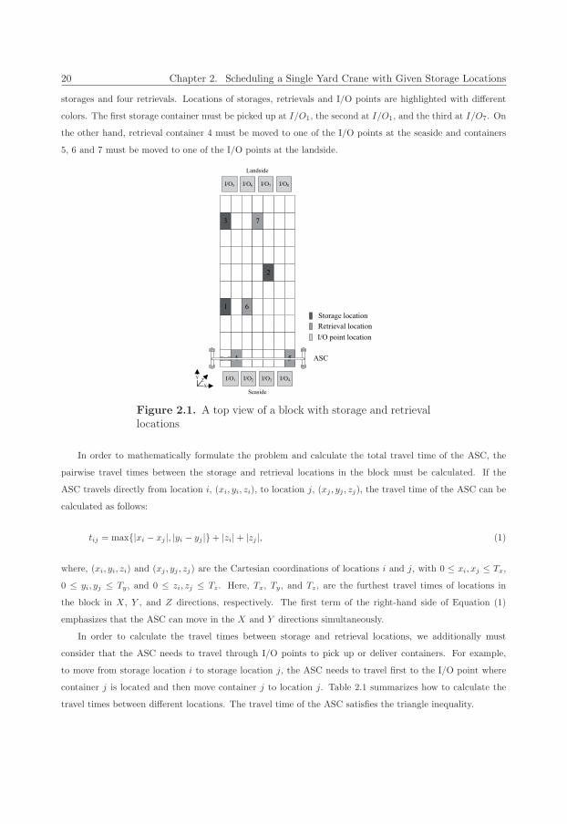
20 Chapter 2. Scheduling a Single Yard Crane with Given Storage Locations
storages and four retrievals. Locations of storages, retrievals and I/O points are highlighted with different
colors. The first storage container must be picked up at I/O1, the second at I/O1, and the third at I/O7. On
the other hand, retrieval container 4 must be moved to one of the I/O points at the seaside and containers
5, 6 and 7 must be moved to one of the I/O points at the landside.
Figure 2.1. A top view of a block with storage and retrievallocations
In order to mathematically formulate the problem and calculate the total travel time of the ASC, the
pairwise travel times between the storage and retrieval locations in the block must be calculated. If the
ASC travels directly from location i, (xi, yi, zi), to location j, (xj , yj , zj), the travel time of the ASC can be
calculated as follows:
tij = max{|xi − xj |, |yi − yj |}+ |zi|+ |zj |, (1)
where, (xi, yi, zi) and (xj , yj , zj) are the Cartesian coordinations of locations i and j, with 0 ≤ xi, xj ≤ Tx,
0 ≤ yi, yj ≤ Ty, and 0 ≤ zi, zj ≤ Tz. Here, Tx, Ty, and Tz, are the furthest travel times of locations in
the block in X, Y , and Z directions, respectively. The first term of the right-hand side of Equation (1)
emphasizes that the ASC can move in the X and Y directions simultaneously.
In order to calculate the travel times between storage and retrieval locations, we additionally must
consider that the ASC needs to travel through I/O points to pick up or deliver containers. For example,
to move from storage location i to storage location j, the ASC needs to travel first to the I/O point where
container j is located and then move container j to location j. Table 2.1 summarizes how to calculate the
travel times between different locations. The travel time of the ASC satisfies the triangle inequality.
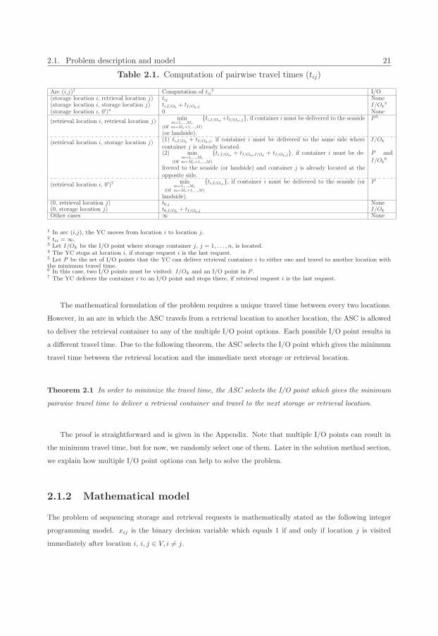
2.1. Problem description and model 21
Table 2.1. Computation of pairwise travel times (tij)
Arc (i,j)1 Computation of tij2 I/O
(storage location i, retrieval location j) tij None(storage location i, storage location j) ti,I/Ok
+ tI/Ok,j I/Ok3
(storage location i, 0′)4 0 None
(retrieval location i, retrieval location j) minm=1,...,Ms
(or m=Ms+1,...,M)
{ti,I/Om+tI/Om,j}, if container imust be delivered to the seaside
(or landside).
P 5
(retrieval location i, storage location j) (1) ti,I/Ok+ tI/Ok,j, if container i must be delivered to the same side where
container j is already located.I/Ok
(2) minm=1,...,Ms
(or m=Ms+1,...,M)
{ti,I/Om + tI/Om,I/Ok+ tI/Ok,j}, if container i must be de-
livered to the seaside (or landside) and container j is already located at theopposite side.
P andI/Ok
6
(retrieval location i, 0′)7 minm=1,...,Ms
(or m=Ms+1,...,M)
{ti,I/Om}, if container i must be delivered to the seaside (or
landside).
P
(0, retrieval location j) t0,j None(0, storage location j) t0,I/Ok
+ tI/Ok,j I/Ok
Other cases ∞ None
1 In arc (i,j), the YC moves from location i to location j.2 tii = ∞.3 Let I/Ok be the I/O point where storage container j, j = 1, . . . , n, is located.4 The YC stops at location i, if storage request i is the last request.5 Let P be the set of I/O points that the YC can deliver retrieval container i to either one and travel to another location withthe minimum travel time.6 In this case, two I/O points must be visited: I/Ok and an I/O point in P .7 The YC delivers the container i to an I/O point and stops there, if retrieval request i is the last request.
The mathematical formulation of the problem requires a unique travel time between every two locations.
However, in an arc in which the ASC travels from a retrieval location to another location, the ASC is allowed
to deliver the retrieval container to any of the multiple I/O point options. Each possible I/O point results in
a different travel time. Due to the following theorem, the ASC selects the I/O point which gives the minimum
travel time between the retrieval location and the immediate next storage or retrieval location.
Theorem 2.1 In order to minimize the travel time, the ASC selects the I/O point which gives the minimum
pairwise travel time to deliver a retrieval container and travel to the next storage or retrieval location.
The proof is straightforward and is given in the Appendix. Note that multiple I/O points can result in
the minimum travel time, but for now, we randomly select one of them. Later in the solution method section,
we explain how multiple I/O point options can help to solve the problem.
2.1.2 Mathematical model
The problem of sequencing storage and retrieval requests is mathematically stated as the following integer
programming model. xij is the binary decision variable which equals 1 if and only if location j is visited
immediately after location i, i, j ∈ V, i �= j.
22 Chapter 2. Scheduling a Single Yard Crane with Given Storage Locations
The objective function is to minimize the total travel time of the ASC:
minimize Z =∑
i∈V \{j,0′}
∑j∈V \{0}
tijxij . (2)
The model has the following constraints.
Visiting all locations and carrying out all requests : Each location must be entered and exited exactly
once. Of course, the starting point has no ingoing arc and the ending point has no outgoing arc:
∑i∈V \{j}
xij = 1, ∀j ∈ V \{0}. (3)
∑j∈V \{i}
xij = 1, ∀i ∈ V \{0′}. (4)
Subtour elimination constraints: The ASC must avoid traveling subtours. Therefore, for any subset of
locations O ⊆ V \{0, 0′}, O �= ∅ where |O| is the size of O, we have the following constraint:
∑i,j∈O
xij ≤ |O| − 1. (5)
All the variables are binary:
xij ∈ {0, 1}, ∀i, j ∈ V. (6)
The problem is defined as an ATSP (tij �= tji), consisting of assignment constraints plus subtour elimina-
tion constraints. In this problem, containers are dispatched on a plane (the block), are picked up or dropped
off at different I/O points located at two ends of the plane, and the crane carrying out the containers can
simultaneously move along the X and Y directions of the plane. Therefore, the travel times are defined based
on the Chebyshev distance (see equation (1)) and the properties of Monge matrix do not hold. As a result,
even in the case of a limited number of I/O points, the enumerative methods which merge subtours by ex-
haustively exchanging arcs among subtours and find the one with the minimum amount of extra travel time
are not applicable. In fact, the complexity of the problem increases in the number of I/O points and requests.
A special case of the problem, where the number of I/O points is not limited (N = M), is NP-hard. This canbe easily proved by polynomial time reduction of the stacker crane problem with uninterrupted movements
on a general graph which has been proven to be NP-hard (Frederickson et al., 1978).
2.2. Solution method 23
2.2 Solution method
A relaxation of the problem is an AP that can be efficiently solved in O(N3) steps where N is the number
of requests (Kuhn, 1955). An optimal AP solution often contains subtours since the subtour elimination
constraint (Equation (5)) may not be satisfied. In order to merge subtours to obtain an optimal solution of
our problem, we first develop some unique properties of the problem. Using these properties, an algorithm
is developed in subsection 2.2.1 to merge subtours. If all subtours have been merged into a single tour,
an optimal solution is found. Otherwise, some subtours have not been merged, and a B&B algorithm is
developed in subsection 2.2.2 to merge all remaining subtours to obtain an optimal solution of our problem.
2.2.1 Merging algorithm
In this phase, we first in subsection 2.2.1 explain how to patch subtours of an optimal AP solution two by
two by swapping arcs visiting a common I/O point. Then, in subsection 2.2.1, we introduce arcs in which
the ASC can has multiple I/O point options to travel from the origins to the destinations of the arcs. These
arcs can be used to create more opportunities to merge subtours. Finally, in subsection 2.2.1, we present the
merging algorithm. We show that the objective value does not change after this merging.
Merging subtours based on an optimal AP solution
In this section, we find some properties of the problem to merge subtours of the AP solution without adding
extra travel time.
Definition 1 The visiting I/O point of an arc is the I/O point that the ASC needs to travel through either
to pick up or to deliver a container in order to travel the arc connecting two requests.
In order to visualize the visiting I/O point of an arc, we need to distinguish carrying and non-carrying
moves. In case of a retrieval request, the ASC starts with a non-carrying move from a storage location (or
an I/O point) to the retrieval location, and then continues with a carrying move from the retrieval location
to an I/O point. In case of a storage request, the ASC starts with a carrying move from an I/O point to the
storage location, and then continues with a non-carrying move from the storage location to an I/O point or
retrieval location. This property is implicitly considered in travel time of different arcs connecting requests,
based on the calculations summarized in Table 2.1.
Figure 2.2b shows carrying and non-carrying moves of the arcs of an optimal AP solution presented in
Figure 2.2a. For clarity, in Figure 2.2b, only the first and second subtours are considered. For example,
storage request 1 is connected to I/O1 by a carrying move and to retrieval request 4 by a non-carrying move.
Furthermore, retrieval request 4 is connected to I/O1 by a carrying move and to storage request 1 by a
non-carrying move. As a result, I/O1 is the visiting I/O point of arc 4x41=1−−−−→ 1.
Arcs in two different subtours that have a common visiting I/O point can be swapped between those
subtours resulting in a merged subtour without extra travel time. These so-called swappable arcs have the
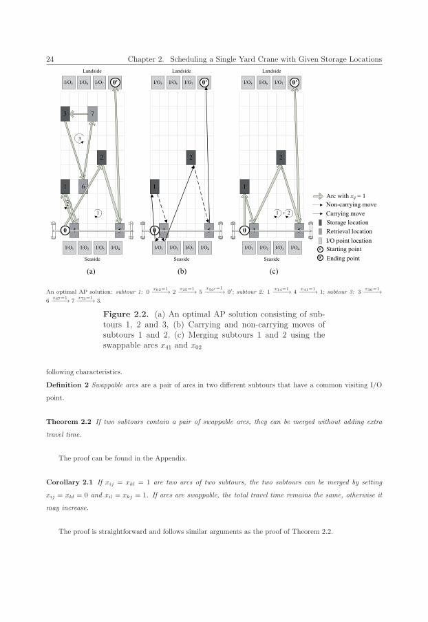
24 Chapter 2. Scheduling a Single Yard Crane with Given Storage Locations
An optimal AP solution: subtour 1: 0x02=1−−−−→ 2
x25=1−−−−→ 5x50′=1−−−−−→ 0′; subtour 2: 1
x14=1−−−−→ 4x41=1−−−−→ 1; subtour 3: 3
x36=1−−−−→6
x67=1−−−−→ 7x73=1−−−−→ 3.
Figure 2.2. (a) An optimal AP solution consisting of sub-tours 1, 2 and 3, (b) Carrying and non-carrying moves ofsubtours 1 and 2, (c) Merging subtours 1 and 2 using theswappable arcs x41 and x02
following characteristics.
Definition 2 Swappable arcs are a pair of arcs in two different subtours that have a common visiting I/O
point.
Theorem 2.2 If two subtours contain a pair of swappable arcs, they can be merged without adding extra
travel time.
The proof can be found in the Appendix.
Corollary 2.1 If xij = xkl = 1 are two arcs of two subtours, the two subtours can be merged by setting
xij = xkl = 0 and xil = xkj = 1. If arcs are swappable, the total travel time remains the same, otherwise it
may increase.
The proof is straightforward and follows similar arguments as the proof of Theorem 2.2.
2.2. Solution method 25
In the optimal AP solution presented in Figure 2.2a, x41 and x02 define a pair of swappable arcs because
both arcs visit I/O1 (follow the carrying moves in Figure 2.2b). Therefore, based on Theorem 2.2, replacing
them with x42 and x01 results in merging subtours 1 and 2 without adding extra travel time. Merged subtour
1+2 is shown in Figure 2.2c: 0x01=1−−−−→ 1
x14=1−−−−→ 4x42=1−−−−→ 2
x25=1−−−−→ 5x50′=1−−−−→ 0′.
Merging subtours using replaceable I/O points
In the previous section, we used the following type of swappable arcs in Theorem 2.2 to patch subtours of an
optimal AP solution.
Definition 3 An arc with a single irreplaceable visiting I/O point is an arc in which the ASC has a unique
visiting I/O point option with the minimum travel time to visit and travel from the origin to the destination
of the arc.
The assumption that all arcs have a single irreplaceable visiting I/O point results in missing some merging
opportunitis. As the last column of Table 2.1 shows, in some arcs, the ASC may be able to visit one of multiple
I/O points with the same travel time. Arcs without any I/O point such as moving from a storage location
to a retrieval location are not a matter of attention here because swappable arcs need to have a common
visiting I/O points. Therefore, we can introduce the following type of arcs.
Definition 4 An arc with replaceable visiting I/O points is an arc in which the ASC has multiple visiting
I/O point options with the minimum travel time to visit and travel from the origin to the destination of the
arc.
Based on the last column of Table 2.1, an arc with replaceable visiting I/O points can be realized if the
request corresponding to the location at the origin of an arc is a retrieval request. The retrieved container
must be delivered to an I/O point which results in the minimum travel time for the ASC in order to travel
from the origin to the destination of the arc (Theorem 2.1). In some cases, multiple I/O points may give
the same minimum travel time one of which can be chosen. Arcs with replaceable visiting I/O points create
extra opportunities to merge subtours.
During the merging algorithm, we check each arc to find out the number of visiting I/O points. However,
in order to speed up the algorithm, we introduce the following theorem which can be used to identify the
types of arcs that always have a single irreplaceable visiting I/O point. The other arcs may have replaceable
or irreplaceable I/O points.
Theorem 2.3 Arc ixij=1−−−−→ j has a single irreplaceable visiting I/O point if:
1. i and j are both storage requests, or
2. i is a retrieval request, j is a storage request and retrieval container i must be delivered to the same
side where storage container j must be picked up.
The proof is given in the Appendix.
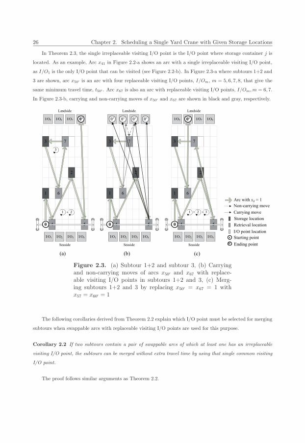
26 Chapter 2. Scheduling a Single Yard Crane with Given Storage Locations
In Theorem 2.3, the single irreplaceable visiting I/O point is the I/O point where storage container j is
located. As an example, Arc x41 in Figure 2.2-a shows an arc with a single irreplaceable visiting I/O point,
as I/O1 is the only I/O point that can be visited (see Figure 2.2-b). In Figure 2.3-a where subtours 1+2 and
3 are shown, arc x50′ is an arc with four replaceable visiting I/O points, I/Om, m = 5, 6, 7, 8, that give the
same minimum travel time, t50′ . Arc x67 is also an arc with replaceable visiting I/O points, I/Om,m = 6, 7.
In Figure 2.3-b, carrying and non-carrying moves of x50′ and x67 are shown in black and gray, respectively.
Figure 2.3. (a) Subtour 1+2 and subtour 3, (b) Carryingand non-carrying moves of arcs x50′ and x67 with replace-able visiting I/O points in subtours 1+2 and 3, (c) Merg-ing subtours 1+2 and 3 by replacing x50′ = x67 = 1 withx57 = x60′ = 1
The following corollaries derived from Theorem 2.2 explain which I/O point must be selected for merging
subtours when swappable arcs with replaceable visiting I/O points are used for this purpose.
Corollary 2.2 If two subtours contain a pair of swappable arcs of which at least one has an irreplaceable
visiting I/O point, the subtours can be merged without extra travel time by using that single common visiting
I/O point.
The proof follows similar arguments as Theorem 2.2.
2.2. Solution method 27
Corollary 2.3 discusses a more general case of this theorem when both swappable arcs have replaceable
visiting I/O points.
Corollary 2.3 If two subtours contain a pair of swappable arcs, both with replaceable visiting I/O points,
using any of the common visiting I/O points, the subtours can be merged without extra travel time.
The proof follows similar arguments as Theorem 2.2.
Corollaries 2.2 and 2.3 state that arcs replacing the swappable arcs should visit one of the common
visiting I/O points. Visiting other I/O points will increase the total travel time, thus these I/O points must
be omitted. An example of Corollary 2.2 is merging subtours 1 and 2 using swappable arcs x41 and x02 where
the single common visiting I/O point is I/O1 (see Figure 2.2). An example of Corollary 2.3 is presented in
Figure 2.3. Swappable arcs of subtours 1+2 and 3 shown in Figure 2.3a are x67 and x50′ . The carrying,
non-carrying moves and replaceable visiting I/O points of these arcs are shown with different colors in Figure
2.3b. Based on Corollary 2.3, common visiting I/O points, I/Om, m = 6, 7, can be used to merge subtours
1+2 and 3. A complete tour is shown in Figure 2.3c. In this solution, I/O6 is for example selected to deliver
the retrieved container 6.
Merging algorithm steps
Having considered different properties of the problem, the merging algorithm can be presented. In the
algorithm, merging subtours will be carried out by using the following arcs consecutively: (1) swappable arcs
with a single irreplaceable visiting I/O point, (2) swappable arcs with replaceable visiting I/O points, and
(3) swappable arcs of which one has a single irreplaceable visiting I/O point and the other has replaceable
visiting I/O points. The reason behind this sequence is as follows:
In case both swappable arcs have a single irreplaceable visiting I/O point, merging two subtours results
in a merged subtour in which the same common visiting I/O point will be visited by the new arcs replacing
the swappable arcs (based on corollary 2.2). This is the ideal case because the subtours are merged without
omitting any I/O point. In the other two cases, the number of common I/O points that will be kept in
the merged subtours determines the sequences. In case swappable arcs have replaceable I/O points, the two
related subtours can be merged using one of the common I/O points (based on corollary 2.3). On the other
hand, in the third case, arcs replacing the swappable arcs visit only a single irreplaceable common visiting
I/O point (based on corollary 2.2). In other words, in the third case only a single common visiting I/O point
can be used to join the merged subtour to the other subtours whereas in the second case at least one common
visiting I/O point exist. Therefore, the second case has priority in subtour merging over the third case.
In the Algorithm (1), Um and U ′m are the sets of all arcs in an optimal AP solution with irreplaceable
and replaceable visiting I/O points respectively, which visit I/Om, m = 1, . . . ,M .
The merging algorithm complexity is O(MN), where N is the total number of requests and M is the
number of I/O points. The complexity of the algorithm comes from identifying each type of arc. We need to
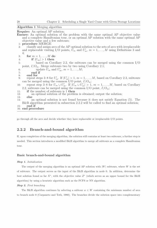
28 Chapter 2. Scheduling a Single Yard Crane with Given Storage Locations
Algorithm 1 Merging algorithm
Require: An optimal AP solution;Ensure: An optimal solution of the problem with the same optimal AP objective value
and a complete Hamiltonian tour, or an optimal AP solution with the same optimal APobjective value and a few subtours;
1: procedure MERGE2: classify and assign arcs of the AP optimal solution to the sets of arcs with irreplaceable
and replaceable visiting I/O points, Um and U ′m, m = 1, . . . ,M using Definitions 3 and
4;3: for m = 1, . . . ,M do4: if |Um| > 1 then5: based on Corollary 2.2, the subtours can be merged using the common I/O
point, I/Om. Merge subtours two by two using Corollary 2.1;6: update Um and U ′
m, m = 1, . . . ,M ;7: end if8: end for9: repeat steps 3–8 for U ′
m. If |U ′m| > 1, m = 1, . . . ,M , based on Corollary 2.3, subtours
can be merged using the common I/O point, I/Om;10: repeat step 3–8 for Um ∪ U ′
m. If |Um ∪ U ′m| > 1, m = 1, . . . ,M , based on Corollary
2.2, subtours can be merged using the common I/O point, I/Om;11: if the number of subtours is 1 then12: an optimal solution of the problem is obtained; output the solution;13: else14: an optimal solution is not found because it does not satisfy Equation (5). The
B&B algorithm presented in subsection 2.2.2 will be called to find an optimal solution;15: end if16: end procedure
go through all the arcs and decide whether they have replaceable or irreplaceable I/O points.
2.2.2 Branch-and-bound algorithm
If, upon completion of the merging algorithm, the solution still contains at least two subtours, a further step is
needed. This section introduces a modified B&B algorithm to merge all subtours as a complete Hamiltonian
tour.
Basic branch-and-bound algorithm
Step 1. Initialization
The output of the merging algorithm is an optimal AP solution with |W | subtours, where W is the set
of subtours. The output serves as the input of the B&B algorithm in node 0. In addition, determine the
best solution found so far X∗, with the objective value Z∗ (which serves as an upper bound for the B&B
algorithm) by using a heuristic algorithm such as the FCFS or NN algorithm.
Step 2. First branching
The B&B algorithm continues by selecting a subtour w ∈ W containing the minimum number of arcs
to branch node 0 (Carpaneto and Toth, 1980). The branches divide the solution space into complementary
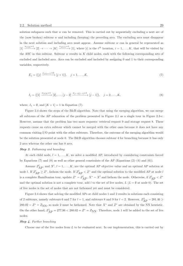
2.2. Solution method 29
solution subspaces such that w can be removed. This is carried out by sequentially excluding a next arc of
the (now broken) subtour w and including (keeping) the preceding arcs. The excluding arcs must disappear
in the next solution and including arcs must appear. Assume subtour w can in general be represented as
[1]x[1][2]=1−−−−−→ [2] → · · · → [K]
x[K][1]=1−−−−−−→ [1], where [i] is the ith location, i = 1, . . . ,K, that will be visited by
the ASC in this subtour. Subtour w results in K child nodes, each with the following corresponding sets of
excluded and included arcs. Arcs can be excluded and included by assigning 0 and 1 to their corresponding
variables, respectively.
Ej = {[j]x[j][j+1]=0−−−−−−−→ [j + 1]}, j = 1, . . . ,K, (7)
Ij = {[1]x[1][2]=1−−−−−→ [2], . . . , [j − 2]
x[j−2][j−1]=1−−−−−−−−→ [j − 1]}, j = 2, . . . ,K, (8)
where, I1 = ∅, and [K + 1] = 1 in Equation (7).
Figure 2.4 shows the steps of the B&B algorithm. Note that using the merging algorithm, we can merge
all subtours of the AP relaxation of the problem presented in Figure 2.1 as a single tour in Figure 2.3-c.
However, assume that the problem has two more requests: retrieval request 9 and storage request 8. These
requests cause an extra subtour which cannot be merged with the other ones because it does not have any
common visiting I/O point with the other subtours. Therefore, the outcome of the merging algorithm would
be the solution presented at node 0. The B&B algorithm chooses subtour 4 for branching because it has only
2 arcs whereas the other one has 8 arcs.
Step 3. Fathoming and bounding
At each child node, l = 1, . . . ,K, we solve a modified AP, introduced by considering constraints forced
by Equations (7) and (8) as well as other general constraints of the AP (Equations (2)–(4) and (6)).
Assume ZlAP, and X l, l = 1, . . . ,K, are the optimal AP objective value and an optimal AP solution at
node l. If ZlAP ≥ Z∗, fathom the node. If Zl
AP < Z∗ and the optimal solution to the modified AP at node l
is a complete Hamiltonian tour, update Z∗ = ZlAP, X
∗ = X l and fathom the node. Otherwise, if ZlAP < Z∗
and the optimal solution is not a complete tour, add l to the set of live nodes, L (L = ∅ at node 0). The set
of live nodes is the set of nodes that are not fathomed yet and must be considered.
Figure 2.4 shows that solving the modified APs at child nodes 1 and 2 results in solutions each consisting
of 2 subtours, namely subtours 6 and 7 for l = 1, and subtours 8 and 9 for l = 2. However, Z2AP = 281.46 ≥
280.02 = Z∗ = ZNN, so node 2 must be fathomed. Note that X∗ and Z∗ are obtained by the NN heuristic.
On the other hand, Z1AP = 277.96 < 280.02 = Z∗ = ZNN. Therefore, node 1 will be added to the set of live
nodes.
Step 4. Further branching
Choose one of the live nodes from L to be evaluated next. In our implementation, this is carried out by
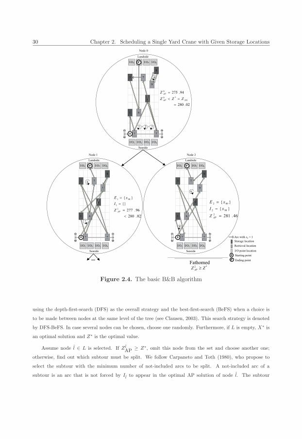
30 Chapter 2. Scheduling a Single Yard Crane with Given Storage Locations
Figure 2.4. The basic B&B algorithm
using the depth-first-search (DFS) as the overall strategy and the best-first-search (BeFS) when a choice is
to be made between nodes at the same level of the tree (see Clausen, 2003). This search strategy is denoted
by DFS-BeFS. In case several nodes can be chosen, choose one randomly. Furthermore, if L is empty, X∗ is
an optimal solution and Z∗ is the optimal value.
Assume node l ∈ L is selected. If Z lAP ≥ Z∗, omit this node from the set and choose another one;
otherwise, find out which subtour must be split. We follow Carpaneto and Toth (1980), who propose to
select the subtour with the minimum number of not-included arcs to be split. A not-included arc of a
subtour is an arc that is not forced by Il to appear in the optimal AP solution of node l. The subtour
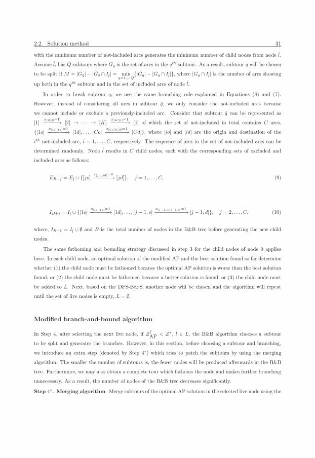
2.2. Solution method 31
with the minimum number of not-included arcs generates the minimum number of child nodes from node l.
Assume l, has Q subtours where Gq is the set of arcs in the qth subtour. As a result, subtour q will be chosen
to be split if M = |Gq| − |Gq ∩ Il| = minq=1,...Q
{|Gq| − |Gq ∩ Il|}, where |Gq ∩ Il| is the number of arcs showing
up both in the qth subtour and in the set of included arcs of node l.
In order to break subtour q, we use the same branching rule explained in Equations (8) and (7).
However, instead of considering all arcs in subtour q, we only consider the not-included arcs because
we cannot include or exclude a previously-included arc. Consider that subtour q can be represented as
[1]x[1][2]=1−−−−−→ [2] → · · · → [K]
x[K][1]=1−−−−−−→ [1] of which the set of not-included in total contains C arcs,
{[1o] x[1o][1d]=1−−−−−−−→ [1d], . . . , [Co]x[Co][Cd]=1−−−−−−−→ [Cd]}, where [io] and [id] are the origin and destination of the
ith not-included arc, i = 1, . . . , C, respectively. The sequence of arcs in the set of not-included arcs can be
determined randomly. Node l results in C child nodes, each with the corresponding sets of excluded and
included arcs as follows:
EB+j = El ∪ {[jo]x[jo][jd]=0−−−−−−→ [jd]}, j = 1, . . . , C, (9)
IB+j = Il ∪ {[1o]x[1o][1d]=1−−−−−−−→ [1d], . . . , [j − 1, o]
x[j−1,o][j−1,d]=1−−−−−−−−−−→ [j − 1, d]}, j = 2, . . . , C, (10)
where, IB+1 = Il ∪ ∅ and B is the total number of nodes in the B&B tree before generating the new child
nodes.
The same fathoming and bounding strategy discussed in step 3 for the child nodes of node 0 applies
here. In each child node, an optimal solution of the modified AP and the best solution found so far determine
whether (1) the child node must be fathomed because the optimal AP solution is worse than the best solution
found, or (2) the child node must be fathomed because a better solution is found, or (3) the child node must
be added to L. Next, based on the DFS-BeFS, another node will be chosen and the algorithm will repeat
until the set of live nodes is empty, L = ∅.
Modified branch-and-bound algorithm
In Step 4, after selecting the next live node, if Z lAP < Z∗, l ∈ L, the B&B algorithm chooses a subtour
to be split and generates the branches. However, in this section, before choosing a subtour and branching,
we introduce an extra step (denoted by Step 4∗) which tries to patch the subtours by using the merging
algorithm. The smaller the number of subtours is, the fewer nodes will be produced afterwards in the B&B
tree. Furthermore, we may also obtain a complete tour which fathoms the node and makes further branching
unnecessary. As a result, the number of nodes of the B&B tree decreases significantly.
Step 4∗. Merging algorithm. Merge subtours of the optimal AP solution in the selected live node using the
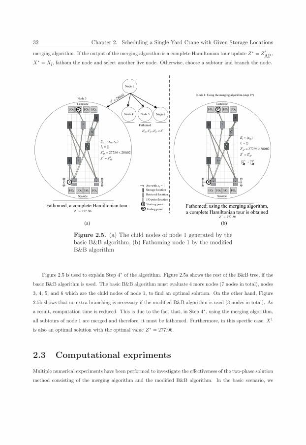
32 Chapter 2. Scheduling a Single Yard Crane with Given Storage Locations
merging algorithm. If the output of the merging algorithm is a complete Hamiltonian tour update Z∗ = Z lAP,
X∗ = Xl, fathom the node and select another live node. Otherwise, choose a subtour and branch the node.
Figure 2.5. (a) The child nodes of node 1 generated by thebasic B&B algorithm, (b) Fathoming node 1 by the modifiedB&B algorithm
Figure 2.5 is used to explain Step 4∗ of the algorithm. Figure 2.5a shows the rest of the B&B tree, if the
basic B&B algorithm is used. The basic B&B algorithm must evaluate 4 more nodes (7 nodes in total), nodes
3, 4, 5, and 6 which are the child nodes of node 1, to find an optimal solution. On the other hand, Figure
2.5b shows that no extra branching is necessary if the modified B&B algorithm is used (3 nodes in total). As
a result, computation time is reduced. This is due to the fact that, in Step 4∗, using the merging algorithm,
all subtours of node 1 are merged and therefore, it must be fathomed. Furthermore, in this specific case, X1
is also an optimal solution with the optimal value Z∗ = 277.96.
2.3 Computational expriments
Multiple numerical experiments have been performed to investigate the effectiveness of the two-phase solution
method consisting of the merging algorithm and the modified B&B algorithm. In the basic scenario, we
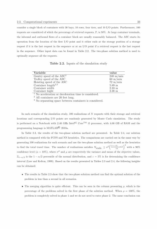
2.3. Computational expriments 33
consider a single block of containers with 30 bays, 10 rows, four tiers, and 10 I/O points. Furthermore, 100
requests are considered of which the percentage of retrieval requests, P, is 50%. At large container terminals,
the inbound and outbound flows of a container block are usually reasonably balanced. The ASC starts its
operation from the location of the first I/O point and it either ends at the storage position of a storage
request if it is the last request in the sequence or at an I/O point if a retrieval request is the last request
in the sequence. Other input data can be found in Table 2.2. The two-phase solution method is used to
optimally sequence all the requests.
Table 2.2. Inputs of the simulation study
Variable valueGantry speed of the ASC1 240 m/minTrolley speed of the ASC 60 m/minHoisting speed of the ASC 72 m/minContainer length2,3 5.89 mContainer width 2.33 mContainer hight 2.38 m1 No acceleration or deceleration time is considered.2 All containers are 20 feet long.3 No separating space between containers is considered.
In each scenario of the simulation study, 100 realizations of N requests with their storage and retrieval
locations and corresponding I/O points are randomly generated by Monte Carlo simulation. The study
is performed on a Notebook with 2.40 GHz Intel� CoreTM i5 processor, with 4.00 GB of RAM and the
programming language is MATLAB� 2010a.
In Table 2.3, the results of the two-phase solution method are presented. In Table 2.4, our solution
method is compared with the FCFS and NN heuristics. The comparisons are carried out in the same way by
generating 100 realizations for each scenario and use the two-phase solution method as well as the heuristics
to find the total travel time. The number of realizations satisfies Nrealz. ≥ σ2(
(1+ε)Z1−α/2
εμ
)2
with a 90%
confidence level (α = 10%), where σ2 and μ are respectively the variance and mean of the objective values,
Z1−α/2 is the 1 − α/2 percentile of the normal distribution, and ε = 5% is for determining the confidence
interval (Law and Kelton, 1999). Based on the results presented in Tables 2.3 and 2.4, the following insights
can be obtained:
� The results in Table 2.3 show that the two-phase solution method can find the optimal solution of the
problem in less than a second in all scenarios.
� The merging algorithm is quite efficient. This can be seen in the column presenting ρ, which is the
percentage of the problems solved in the first phase of the solution method. When ρ = 100%, the
problem is completely solved in phase 1 and we do not need to enter phase 2. The same conclusion can
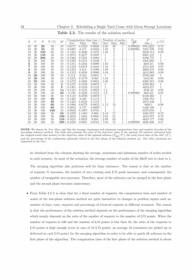
34 Chapter 2. Scheduling a Single Yard Crane with Given Storage Locations
Table 2.3. The results of the solution method
X Y N P (%) MComputation time (sec.) Number of nodes Z∗
APZ∗
Z∗ρ (%)
Ave Max Min Ave Max Min (Sec.)10 30 20 50 10 0.0177 0.1353 0.0049 3.88 39 1 0.999923 976.4222 0.7310 30 50 50 10 0.0397 0.171 0.0256 1.32 9 1 0.999995 2325.709 0.9310 30 100 50 10 0.1321 0.3936 0.1072 1.04 5 1 1 4650.213 0.9910 30 150 50 10 0.2973 0.3377 0.2397 1 1 1 1 6965.121 110 30 200 50 10 0.5462 0.7231 0.4062 1 1 1 1 9190.737 15 30 100 50 10 0.1295 0.1554 0.1038 1 1 1 1 4595.805 16 30 100 50 10 0.1315 0.4104 0.0999 1.04 5 1 1 4605.67 0.997 30 100 50 10 0.1419 0.6872 0.1034 1.16 9 1 1 4551.678 0.978 30 100 50 10 0.1353 0.413 0.1086 1.08 5 1 1 4609.479 0.989 30 100 50 10 0.1312 0.3934 0.0968 1.04 5 1 1 4612.963 0.9910 20 100 50 10 0.112 0.165 0.0851 1 1 1 1 3788.589 110 40 100 50 10 0.1215 0.3179 0.094 1.04 5 1 1 5410.98 0.9910 50 100 50 10 0.1272 0.4288 0.0931 1.08 5 1 1 6360.285 0.9810 30 100 50 2 0.1237 0.1593 0.0878 1 1 1 1 4760.263 110 30 100 50 8 0.1301 0.1524 0.1123 1 1 1 1 4633.471 110 30 100 50 14 0.1415 0.4124 0.0923 1.2 5 1 1 4592.33 0.9510 30 100 50 20 0.139 0.4238 0.1054 1.2 5 1 0.999998 4645.63 0.9510 30 100 0 10 0.1147 0.3789 0.0978 1 1 1 1 6130.303 110 30 100 20 10 0.1401 0.248 0.1113 1 1 1 1 5330.784 110 30 100 40 10 0.1324 0.2342 0.1116 1 1 1 1 4672.246 110 30 100 60 10 0.1068 0.8279 0.0822 1.12 13 1 1 4800.1 0.9910 30 100 80 10 0.0952 0.137 0.0809 1 1 1 1 5436.168 110 30 100 100 10 0.0942 0.1807 0.0781 1 1 1 1 6197.658 110 30 100 50 50 0.1976 1.1485 0.093 2.44 17 1 1 4595.972 0.7510 30 100 50 100 0.2034 1.3404 0.0865 2.62 21 1 1 4624.975 0.7910 30 100 50 150 0.3221 4.5623 0.084 4.88 83 1 1 4633.177 0.6810 30 100 50 200 0.4459 3.8641 0.0761 7.02 75 1 0.999999 4620.406 0.57
NOTE. We denote by Ave, Max, and Min the average, maximum and minimum computation time and number of nodes of thetwo-phase solution method. The table also presents the ratio of the objective value of the optimal AP solution (obtained fromthe original travel time matrix) to the objective value of the optimal solution (Z∗
AP/Z∗), the total travel time of the ASC (Z∗),
and the percentage of the realizations optimally solved in the first phase of the solution method (ρ). The other notations areexplained in the text.
be obtained from the columns showing the average, maximum and minimum number of nodes needed
in each scenario. In most of the scenarios, the average number of nodes of the B&B tree is close to 1.
The merging algorithm also performs well for large instances. The reason is that as the number
of requests N increases, the number of arcs visiting each I/O point increases, and consequently the
number of swappable arcs increases. Therefore, most of the subtours can be merged in the first phase
and the second phase becomes unnecessary.
� From Table 2.3 it is clear that for a fixed number of requests, the computation time and number of
nodes of the two-phase solution method are quite insensitive to changes in problem inputs such as:
number of bays, rows, requests and percentage of retrieval requests in different scenarios. The reason
is that the performance of the solution method depends on the performance of the merging algorithm
which mainly depends on the ratio of the number of requests to the number of I/O points. When the
number of requests is 100 and the number of I/O points is less than 10, the ratio of the requests to
I/O points is high enough (even in case of 10 I/O points, on average 10 containers are picked up or
delivered at each I/O point) for the merging algorithm in order to be able to patch all subtours in the
first phase of the algorithm. The computation time of the first phase of the solution method is about
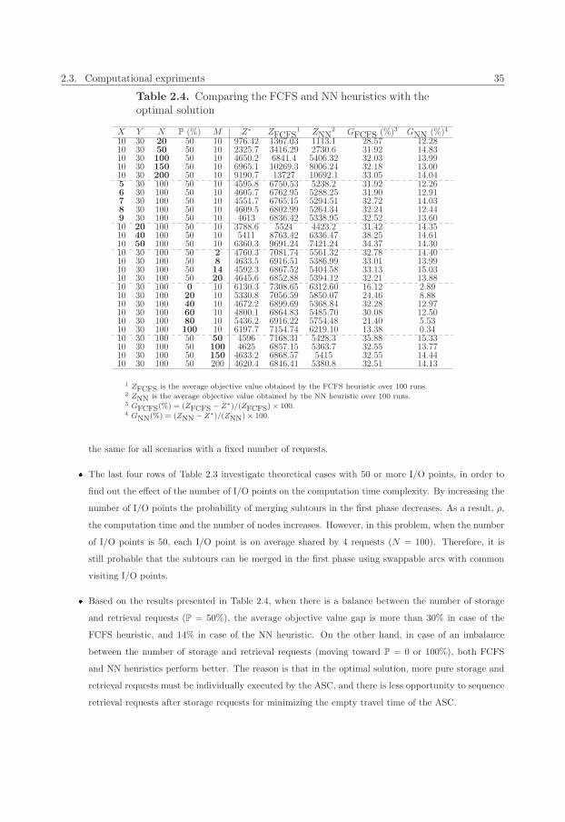
2.3. Computational expriments 35
Table 2.4. Comparing the FCFS and NN heuristics with theoptimal solution
X Y N P (%) M Z∗ ZFCFS1 ZNN
2 GFCFS (%)3 GNN (%)4
10 30 20 50 10 976.42 1367.03 1113.1 28.57 12.2810 30 50 50 10 2325.7 3416.29 2730.6 31.92 14.8310 30 100 50 10 4650.2 6841.4 5406.32 32.03 13.9910 30 150 50 10 6965.1 10269.3 8006.24 32.18 13.0010 30 200 50 10 9190.7 13727 10692.1 33.05 14.045 30 100 50 10 4595.8 6750.53 5238.2 31.92 12.266 30 100 50 10 4605.7 6762.95 5288.25 31.90 12.917 30 100 50 10 4551.7 6765.15 5294.51 32.72 14.038 30 100 50 10 4609.5 6802.99 5264.34 32.24 12.449 30 100 50 10 4613 6836.42 5338.95 32.52 13.6010 20 100 50 10 3788.6 5524 4423.2 31.42 14.3510 40 100 50 10 5411 8763.42 6336.47 38.25 14.6110 50 100 50 10 6360.3 9691.24 7421.24 34.37 14.3010 30 100 50 2 4760.3 7081.74 5561.32 32.78 14.4010 30 100 50 8 4633.5 6916.51 5386.99 33.01 13.9910 30 100 50 14 4592.3 6867.52 5404.58 33.13 15.0310 30 100 50 20 4645.6 6852.88 5394.12 32.21 13.8810 30 100 0 10 6130.3 7308.65 6312.60 16.12 2.8910 30 100 20 10 5330.8 7056.59 5850.07 24.46 8.8810 30 100 40 10 4672.2 6899.69 5368.84 32.28 12.9710 30 100 60 10 4800.1 6864.83 5485.70 30.08 12.5010 30 100 80 10 5436.2 6916.22 5754.48 21.40 5.5310 30 100 100 10 6197.7 7154.74 6219.10 13.38 0.3410 30 100 50 50 4596 7168.31 5428.3 35.88 15.3310 30 100 50 100 4625 6857.15 5363.7 32.55 13.7710 30 100 50 150 4633.2 6868.57 5415 32.55 14.4410 30 100 50 200 4620.4 6846.41 5380.8 32.51 14.13
1 ZFCFS is the average objective value obtained by the FCFS heuristic over 100 runs.2 ZNN is the average objective value obtained by the NN heuristic over 100 runs.3 GFCFS(%) = (ZFCFS − Z∗)/(ZFCFS)× 100.4 GNN(%) = (ZNN − Z∗)/(ZNN)× 100.
the same for all scenarios with a fixed number of requests.
� The last four rows of Table 2.3 investigate theoretical cases with 50 or more I/O points, in order to
find out the effect of the number of I/O points on the computation time complexity. By increasing the
number of I/O points the probability of merging subtours in the first phase decreases. As a result, ρ,
the computation time and the number of nodes increases. However, in this problem, when the number
of I/O points is 50, each I/O point is on average shared by 4 requests (N = 100). Therefore, it is
still probable that the subtours can be merged in the first phase using swappable arcs with common
visiting I/O points.
� Based on the results presented in Table 2.4, when there is a balance between the number of storage
and retrieval requests (P = 50%), the average objective value gap is more than 30% in case of the
FCFS heuristic, and 14% in case of the NN heuristic. On the other hand, in case of an imbalance
between the number of storage and retrieval requests (moving toward P = 0 or 100%), both FCFS
and NN heuristics perform better. The reason is that in the optimal solution, more pure storage and
retrieval requests must be individually executed by the ASC, and there is less opportunity to sequence
retrieval requests after storage requests for minimizing the empty travel time of the ASC.
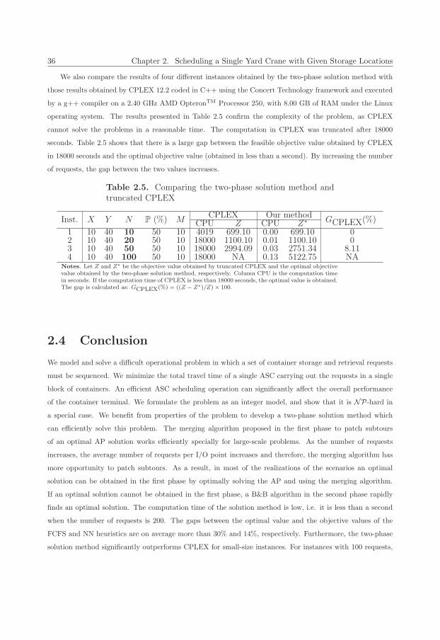
36 Chapter 2. Scheduling a Single Yard Crane with Given Storage Locations
We also compare the results of four different instances obtained by the two-phase solution method with
those results obtained by CPLEX 12.2 coded in C++ using the Concert Technology framework and executed
by a g++ compiler on a 2.40 GHz AMD OpteronTM Processor 250, with 8.00 GB of RAM under the Linux
operating system. The results presented in Table 2.5 confirm the complexity of the problem, as CPLEX
cannot solve the problems in a reasonable time. The computation in CPLEX was truncated after 18000
seconds. Table 2.5 shows that there is a large gap between the feasible objective value obtained by CPLEX
in 18000 seconds and the optimal objective value (obtained in less than a second). By increasing the number
of requests, the gap between the two values increases.
Table 2.5. Comparing the two-phase solution method andtruncated CPLEX
Inst. X Y N P (%) MCPLEX Our method
GCPLEX(%)CPU Z CPU Z∗1 10 40 10 50 10 4019 699.10 0.00 699.10 02 10 40 20 50 10 18000 1100.10 0.01 1100.10 03 10 40 50 50 10 18000 2994.09 0.03 2751.34 8.114 10 40 100 50 10 18000 NA 0.13 5122.75 NA
Notes. Let Z and Z∗ be the objective value obtained by truncated CPLEX and the optimal objectivevalue obtained by the two-phase solution method, respectively. Column CPU is the computation timein seconds. If the computation time of CPLEX is less than 18000 seconds, the optimal value is obtained.The gap is calculated as: GCPLEX(%) = ((Z − Z∗)/Z)× 100.
2.4 Conclusion
We model and solve a difficult operational problem in which a set of container storage and retrieval requests
must be sequenced. We minimize the total travel time of a single ASC carrying out the requests in a single
block of containers. An efficient ASC scheduling operation can significantly affect the overall performance
of the container terminal. We formulate the problem as an integer model, and show that it is NP-hard in
a special case. We benefit from properties of the problem to develop a two-phase solution method which
can efficiently solve this problem. The merging algorithm proposed in the first phase to patch subtours
of an optimal AP solution works efficiently specially for large-scale problems. As the number of requests
increases, the average number of requests per I/O point increases and therefore, the merging algorithm has
more opportunity to patch subtours. As a result, in most of the realizations of the scenarios an optimal
solution can be obtained in the first phase by optimally solving the AP and using the merging algorithm.
If an optimal solution cannot be obtained in the first phase, a B&B algorithm in the second phase rapidly
finds an optimal solution. The computation time of the solution method is low, i.e. it is less than a second
when the number of requests is 200. The gaps between the optimal value and the objective values of the
FCFS and NN heuristics are on average more than 30% and 14%, respectively. Furthermore, the two-phase
solution method significantly outperforms CPLEX for small-size instances. For instances with 100 requests,
2.4. Conclusion 37
CPLEX cannot obtain a feasible solution after five hours.
The model developed in this paper can be extended in several directions. We assume that containers
do not have any precedence constraints. However, in reality, many issues such as the priority of seaside
operations to landside operations, the arrival time of different modes of transport, and ensuring the stability
of the ship impose precedence constraints to the model. Furthermore, we consider that all storage containers
are available at the I/O points and a retrieval container can be dropped off at the same I/O point from where
another container has to be stacked in the block. But safety regulations and space availability cause some
limitations. Extra constraints are required to model reality. Finally, one may study an online version of the
model where the list of requests is updated in some time periods. Some of these issues are tackled in the
next chapters.
38 Chapter 2. Scheduling a Single Yard Crane with Given Storage Locations
Appendix
2.A Proof of Theorem 2.1
Choosing the I/O point which minimizes the travel time doesn’t affect the optimal sequence of requests.
Let tij be the travel time between locations i and j in an optimal solution. If tij , is larger than t′ij , then
the optimal solution can be improved by replacing tij with t′ij . As a result, in order to have the minimum
objective value, the minimum travel time must be always selected for every arc. �
2.B Proof of Theorem 2.2
Consider two subtours resulting from an optimal AP solution with the swappable arcs xkl = 1 and xrs = 1
and the common visiting I/O point, I/Om. By setting arcs xkl = xrs = 0 and xks = xrl = 1, we can show
that subtours are merged without extra travel time.
The objective function of the problem can be shown as follows:
minZ =∑
i∈V \{j,0′,r,k}
∑j∈V \{0,l,s}
tijxij + tklxkl + trsxrs + tksxks + trlxrl, (11)
Before merging, xkl = xrs = 1 and xks = xrl = 0, so ZBefore =∑
i∈V \{j,0′,r,k}∑
j∈V \{0,l,s} tijxij + tkl +
trs. On the other hand, from Table 2.1, tkl = tk,I/Om+ tI/Om,l and trs = tr,I/Om
+ tI/Om,s. Consequently,
ZBefore =∑
i∈V \{j,0′,r,k}∑
j∈V \{0,l,s} tijxij + tkl + trs =∑
i∈V \{j,0′,r,k}∑
j∈V \{0,l,s} tijxij +
tk,I/Om+ tI/Om,l + tr,I/Om
+ tI/Om,s.
After merging, xkl = xrs = 0 and xks = xrl = 1, so ZAfter =∑
i∈V \{j,0′,r,k}∑
j∈V \{0,l,s} tijxij +
tks + trl. From Table 2.1, we have tks = tk,I/Om+ tI/Om,s and trl = tr,I/Om
+ tI/Om,l, therefore ZAfter =∑i∈V \{j,0′,r,k}
∑j∈V \{0,l,s} tijxij + tk,I/Om
+ tI/Om,s + tr,I/Om+ tI/Om,l = ZBefore. �
2.C Proof of Theorem 2.3
The proof follows from the calculations of Table 2.1. Each case will be proven separately. Note that this
theorem is not bi-conditional, which means that if an arc has a single visiting I/O point, it is not necessarily
the following types of arcs.
Case 1: consider storage request j is immediately after storage request i. Furthermore, I/Ol is the I/O
point where container j must be picked up. Obviously, traveling to an I/O point, I/Ol′ , doesn’t give the
minimum travel time because the ASC must travel to I/Ol, and tI/Ol,I/Ol′ will be added to the total travel
time of the ASC.
2.C. Proof of Theorem 2.3 39
Case 2: consider storage request j is immediately after retrieval request i. Furthermore I/Ol is the I/O
point where container j must be picked up and I/Ol′ is the I/O point where container i will be delivered.
If container i must be delivered into the same side that the storage container is currently located in an I/O
point, the travel time of the ASC is minimum, if I/Ol = I/Ol′ . In words, the container must be delivered to
the same I/O point where the other container must be picked up. If I/Ol �= I/Ol′ , then we add tI/Ol,I/Ol′
to the total travel time of the ASC. �

Chapter 3
Scheduling a Single Yard Crane with
Flexible Storage Locations∗
In Chapter 2, we studied the problem of scheduling an automated stacking crane (ASC) to carry out a set
of storage and retrieval requests in a single block of containers. We considered that in the case of a retrieval
request, the ASC picks up a container from a location in the block and drops it off in an input/output (I/O)
point, whereas in the case of a storage request, the ASC picks up a container from an I/O point and drops
it off at a given location. In this chapter, we study an extension where multiple open locations are available
to stack the storage container. Since container yard operators often physically separate containers based on
criteria such as destination and weight, a set of suitable open locations are available to stack the container.
Obviously, a single location may be suitable for stacking different containers, and thus sets of open locations
may overlap. Figure 3.1b is a top view of a block of containers with multiple storage and retrieval locations.
The sets of open locations available for different storage containers are highlighted by the contours.
We study where to stack storage containers while sequencing a given number of requests in a single
block of containers. The objective is to minimize the travel time of the ASC carrying out the requests. We
formulate the problem as a generalized asymmetric traveling salesman problem (GATSP). In this formulation,
locations in the overlap of multiple sets make the problem more complex. For such open locations, we need
extra constraints to avoid selecting one of them for stacking more than a single storage container. The
GATSP is NP-hard, and the extra constraints increase the complexity even more. We propose a three-phase
solution method to optimally solve the problem. The main idea of the algorithm is to simplify the problem
to an ATSP and use its optimal solution to obtain an optimal GATSP solution. An optimal ATSP solution
can be quickly obtained by the solution method proposed in Chapter 2, which uses the particular structure
of the problem, namely the I/O points to obtain a complete tour. In the first phase of our algorithm, we
∗This chapter is based on Gharehgozli et al. (2012b)
41
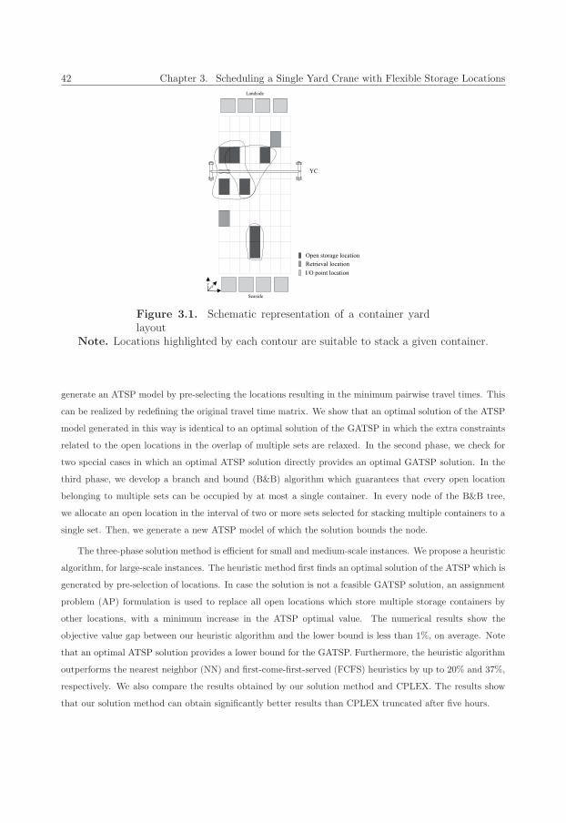
42 Chapter 3. Scheduling a Single Yard Crane with Flexible Storage Locations
Figure 3.1. Schematic representation of a container yardlayout
Note. Locations highlighted by each contour are suitable to stack a given container.
generate an ATSP model by pre-selecting the locations resulting in the minimum pairwise travel times. This
can be realized by redefining the original travel time matrix. We show that an optimal solution of the ATSP
model generated in this way is identical to an optimal solution of the GATSP in which the extra constraints
related to the open locations in the overlap of multiple sets are relaxed. In the second phase, we check for
two special cases in which an optimal ATSP solution directly provides an optimal GATSP solution. In the
third phase, we develop a branch and bound (B&B) algorithm which guarantees that every open location
belonging to multiple sets can be occupied by at most a single container. In every node of the B&B tree,
we allocate an open location in the interval of two or more sets selected for stacking multiple containers to a
single set. Then, we generate a new ATSP model of which the solution bounds the node.
The three-phase solution method is efficient for small and medium-scale instances. We propose a heuristic
algorithm, for large-scale instances. The heuristic method first finds an optimal solution of the ATSP which is
generated by pre-selection of locations. In case the solution is not a feasible GATSP solution, an assignment
problem (AP) formulation is used to replace all open locations which store multiple storage containers by
other locations, with a minimum increase in the ATSP optimal value. The numerical results show the
objective value gap between our heuristic algorithm and the lower bound is less than 1%, on average. Note
that an optimal ATSP solution provides a lower bound for the GATSP. Furthermore, the heuristic algorithm
outperforms the nearest neighbor (NN) and first-come-first-served (FCFS) heuristics by up to 20% and 37%,
respectively. We also compare the results obtained by our solution method and CPLEX. The results show
that our solution method can obtain significantly better results than CPLEX truncated after five hours.
43
Scheduling an ASC to carry out storage and retrieval requests can generally be modeled as an ATSP
or one of its special cases such as the rural postman problem, or Chinese postman problem, depending
on the properties of the problem (see Chapter 2). These papers merely focus on sequencing storage and
retrieval requests and assume that storage locations are already selected by other models (for example, see
Kim et al., 2000, Dekker et al., 2007). However, the decisions made in one problem substantially affect the
decisions in the other problem. Intuitively, given different storage locations may result in different sequences
of performing requests, and vice versa. Scheduling an ASC to carry out storage and retrieval requests in a
block with multiple open locations incorporating the storage location problem can be modeled as a GATSP.
Contrary to the dense literature of the ATSP and symmetric TSP (see for example Applegate et al. (2007)
and Laporte (1992) for an overview on the TSP or Burkard et al. (1998) for an overview on solvable cases),
the GATSP problem has been only considered in a few papers (Fischetti et al., 1997, Laporte et al., 1987,
Noon and Bean, 1991). In the GATSP, multiple sets of locations exist and the problem calls for a tour
passing at least one location of each set in such a way that the total travel time is minimized. If the tour
is forced to pass exactly a single location of each set, the resulting problem is sometimes called E-GATSP,
where E stands for equality. Note that in this chapter, sets of open locations can overlap. In previous more
theoretical papers, sets of open locations either do not overlap, or if they do, all of the overlapping sets are
visited simultaneously by selecting one of the locations in the overlap of some sets. However, in our problem,
a separate location of each set has to appear in a feasible solution.
Laporte et al. (1987) are among the pioneers to study the GATSP. They propose a B&B algorithm to
solve the problem. The core idea of the B&B algorithm is solving the AP relaxation of the problem and
removing the infeasibility. An optimal AP solution may generate an infeasible GATSP solution because (1)
some sets are not visited, and/or (2) multiple subtours exist in the solution. Laporte et al. (1987) force the
tour to visit a not-visited set by requiring a location of that set in the solution. A subtour is avoided by
forbidding one of its arcs and requiring the others to appear in the solution. As a result, in each node of the
B&B algorithm, an AP requiring and forbidding some nodes and arcs is solved. The algorithm is designed
to first include all sets and then remove subtours. In fact, the B&B algorithm is an extension of the B&B
algorithm previously proposed by Carpaneto and Toth (1980) to solve the ATSP by removing the subtours
of the AP relaxation. The latter algorithm was later improved by Miller and Pekny (1991) and Carpaneto
et al. (1995) who propose two merging algorithms to patch subtours in each node and decrease the number
of branches. Noon and Bean (1991) also propose a similar B&B algorithm to solve the GATSP. To enhance
the performance of the B&B algorithm, they first use Lagrangian relaxation to improve the ATSP and AP
bounds. Second, in order to reduce the density of the distance matrix, some of the locations and arcs are
eliminated using the reduced costs. Furthermore, they develop a heuristic algorithm to obtain an upper
bound to fathom some of the nodes.
Fischetti et al. (1995) study the facial structure of the GTSP and E-GTSP polytopes where sets of
locations do not overlap and pairwise travel times are symmetric. Using the theoretical foundation of the
44 Chapter 3. Scheduling a Single Yard Crane with Flexible Storage Locations
paper, they then develop a branch-and-cut algorithm to solve the GTSP (Fischetti et al., 1997). The solution
method uses a B&B scheme. In each node, an LP relaxation of the problem is solved while adding some valid
inequalities. Valid inequalities tighten the solution space of the problem in order to obtain a feasible integer
solution.
The main contribution of this chapter is twofold. We model and solve the simultaneous request scheduling
and storage location selection problem, which is relevant in practice to use the highly utilized ASC efficiently.
The algorithm proposed to solve the problem is new. In the first phase of the algorithm, we use the I/O
points to simplify the problem to an ATSP model by preselecting open locations, which differs from previous
methods (for example, see Dimitrijevic and Saric, 1997, Lien et al., 1993). Furthermore, the specific structure
of the problem, which requires a distinct open location for each storage container, allows us to define a new
B&B algorithm in the third phase of the solution method. In our B&B algorithm, branching is carried
out in order to assign a location in the overlap of multiple sets selected for storing multiple containers to a
single set, so that a separate location of each set can be selected. The method is fast for different sizes of
the problem if sets of open locations do not overlap. An accurate heuristic algorithm is proposed to solve
large-scale problems. The methods are sufficiently general to be applied to other GATSP problems with a
similar structure.
The rest of this chapter is organized as follows. In Section 3.1, we describe the technical aspects of the
problem and present the mathematical model. In Section 3.2, the solution method is developed. Section 3.3
presents numerical results. Finally, in Section 3.4, we conclude the chapter.
3.1 Problem description and model
We seek to determine the sequence to carry out n storage requests and N − n retrieval requests in a single
block of containers consisting of X rows, Y bays, Z tiers and M I/O points. I/Om is the location of the mth
I/O point at the seaside, m = 1, . . . ,Ms, or at the landside, m = Ms + 1, . . . ,M . Let R be the set of all
storage and retrieval requests. The objective is to minimize the total travel time of a single ASC performing
these requests. The ASC can only carry a single container at a time. From a given starting point, the ASC
can perform the requests in any sequence in order to minimize total travel time. We denote by 0 and 0′,
respectively, the starting and ending locations of the ASC which can be anywhere in the block. Containers
can be of different sizes (i.e. 20 or 40 feet) and leave or arrive at the container terminal by truck, train or
ship. In addition, containers should not be dropped off in temporary locations within the block.
Every storage or retrieval request r ∈ R = {1, . . . , N} corresponds to a unique container. For storage
request r, a ASC moves a container from the I/O point where it is initially located to a location i in the block
selected from a given set Lr of available open locations. For retrieval request r, a ASC moves a container
from location j in the block to an I/O point at its destination side. For ease of notation, we write that
location j of retrieval request r belongs to Lr. Thus, the set V of all locations can be defined as:
3.1. Problem description and model 45
V = {1, . . . , |L1|︸ ︷︷ ︸L1
, |L1|+ 1, . . . , |L1|+ |L2|︸ ︷︷ ︸L2
, . . . ,n−1∑i=1
|Li|+ 1, . . . ,n∑
i=1
|Li|︸ ︷︷ ︸Ln
,
n∑i=1
|Li|+ 1
︸ ︷︷ ︸Ln+1
, . . . ,
n∑i=1
|Li|+N − n
︸ ︷︷ ︸LN
,
0︸︷︷︸L0
, 0′︸︷︷︸L0′
}.
in which Lr consists of |Lr| ≥ 1 locations for r = 1, . . . , n, but only one location for r = n+1, . . . , N . For each
storage location in V lying in the overlap of multiple sets, a copy is created for each set to which it belongs.
The copy locations will be used in the next section to model the constraints associated with locations in the
overlap areas.
Storage and retrieval locations as well as destination sides of retrieval containers and I/O points of
storage containers are known; in practice, they are determined at a higher hierarchical planning level. This
level focuses on minimizing the number of reshufflings (De Castillo and Daganzo, 1993, Kim et al., 2000)
and speeding up the loading and unloading process of a ship (Kim and Kim, 1999a, Vis and Roodbergen,
2009). Due to the abundance of internal transport vehicles (like AGVs and chassis) to pick up containers at
the seaside and landside, retrieved containers can be delivered to any I/O point at each side. Because of the
same reason, retrieval containers can be quickly moved away from all I/O points, and they can therefore be
delivered to the same I/O point that a storage container has to be picked up. The other issue is that storage
and retrieval locations do not coincide. This is reasonable since N is usually much smaller than the block size,
the block utilization is often fairly low, and container terminal operators usually separate containers based
on destination and type. Finally, we assume that containers do not have explicit precedence constraints.
This assumption is based on the fact that all containers are categorized into several precedence groups (for
example, based on their latest departure times) and we can consider the sequencing problem group by group.
In Chapter 4, we present an extension of the problem in which precedence constraints are considered.
We use figure 3.2 to explain some of the notations. This figure shows a top view of a block (X = 7,
Y = 10, and Z = 4) with 3 storages, and 2 retrievals. For storage requests 1, 2, and 3, the sets of open
storage locations are L1 = {1, 2}, L2 = {3, 4, 5, 6}, and L3 = {7, 8, 9}, respectively. Location 7 is a copy of
location 4 and location 8 is a copy of location 6. For retrieval requests 4 and 5, L4 = {10}, and L5 = {11},respectively.
In order to mathematically formulate the problem and calculate the total travel time of the ASC, we
must first calculate the pairwise travel times between the storage and retrieval locations in the block. If the
ASC travels directly from location i, (xi, yi, zi), to location j, (xj , yj , zj), the travel time of the ASC can be
calculated as follows:
tij = max{|xi − xj |, |yi − yj |}+ |zi|+ |zj |, (1)
where, (xi, yi, zi) and (xj , yj , zj) are the Cartesian coordinates of locations i and j, with 0 ≤ xi, xj ≤ Tx,
0 ≤ yi, yj ≤ Ty, and 0 ≤ zi, zj ≤ Tz. Here, Tx, Ty, and Tz, are the farthest travel times of the ASC in
the block in X, Y , and Z directions, respectively. The maximum in the first term of the right-hand side
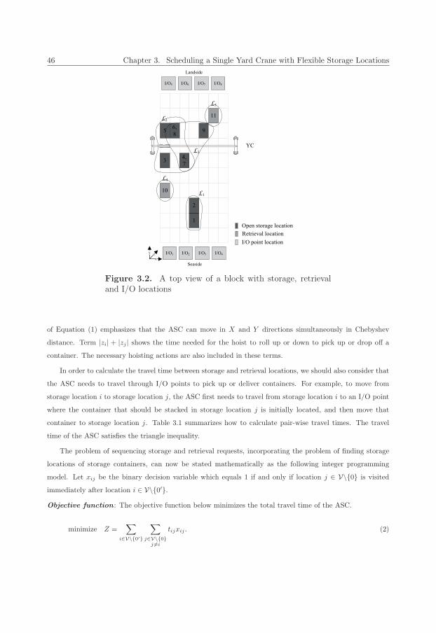
46 Chapter 3. Scheduling a Single Yard Crane with Flexible Storage Locations
Figure 3.2. A top view of a block with storage, retrievaland I/O locations
of Equation (1) emphasizes that the ASC can move in X and Y directions simultaneously in Chebyshev
distance. Term |zi| + |zj | shows the time needed for the hoist to roll up or down to pick up or drop off a
container. The necessary hoisting actions are also included in these terms.
In order to calculate the travel time between storage and retrieval locations, we should also consider that
the ASC needs to travel through I/O points to pick up or deliver containers. For example, to move from
storage location i to storage location j, the ASC first needs to travel from storage location i to an I/O point
where the container that should be stacked in storage location j is initially located, and then move that
container to storage location j. Table 3.1 summarizes how to calculate pair-wise travel times. The travel
time of the ASC satisfies the triangle inequality.
The problem of sequencing storage and retrieval requests, incorporating the problem of finding storage
locations of storage containers, can now be stated mathematically as the following integer programming
model. Let xij be the binary decision variable which equals 1 if and only if location j ∈ V\{0} is visited
immediately after location i ∈ V\{0′}.Objective function : The objective function below minimizes the total travel time of the ASC.
minimize Z =∑
i∈V\{0′}
∑j∈V\{0}
j �=i
tijxij . (2)
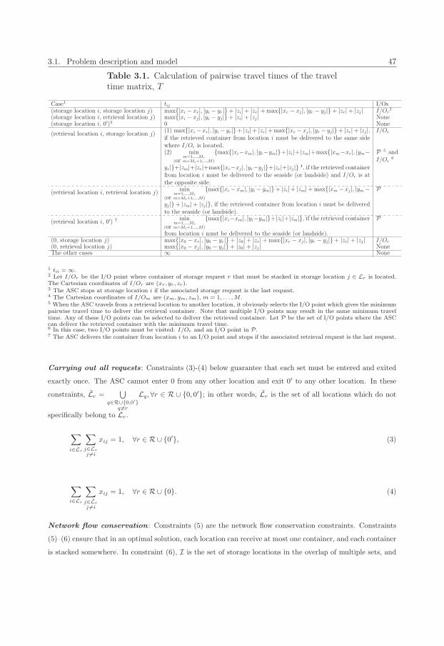
3.1. Problem description and model 47
Table 3.1. Calculation of pairwise travel times of the traveltime matrix, T
Case1 tij I/Os(storage location i, storage location j) max{|xi − xr|, |yi − yr|}+ |zi|+ |zr|+max{|xr − xj|, |yr − yj|}+ |zr|+ |zj| I/Or
2
(storage location i, retrieval location j) max{|xi − xj|, |yi − yj|}+ |zi|+ |zj| None(storage location i, 0′)3 0 None
(retrieval location i, storage location j)(1) max{|xi− xr|, |yi− yr|}+ |zi|+ |zr|+max{|xr − xj|, |yr − yj|}+ |zr|+ |zj|,if the retrieved container from location i must be delivered to the same sidewhere I/Or is located.
I/Or
(2) minm=1,...,Ms
(or m=Ms+1,...,M)
{max{|xi−xm|, |yi−ym|}+|zi|+|zm|+max{|xm−xr|, |ym−
yr|}+|zm|+|zr|+max{|xr−xj|, |yr−yj|}+|zr|+|zj|} 4, if the retrieved containerfrom location i must be delivered to the seaside (or landside) and I/Or is atthe opposite side.
P 5 andI/Or
6
(retrieval location i, retrieval location j)min
m=1,...,Ms
(or m=Ms+1,...,M)
{max{|xi − xm|, |yi − ym|}+ |zi|+ |zm|+max{|xm − xj|, |ym −
yj|}+ |zm|+ |zj|}, if the retrieved container from location i must be deliveredto the seaside (or landside).
P
(retrieval location i, 0′) 7 minm=1,...,Ms
(or m=Ms+1,...,M)
{max{|xi−xm|, |yi−ym|}+|zi|+|zm|}, if the retrieved container
from location i must be delivered to the seaside (or landside).
P
(0, storage location j) max{|x0 − xr|, |y0 − yr|}+ |z0|+ |zr|+max{|xr − xj|, |yr − yj|}+ |zr|+ |zj| I/Or
(0, retrieval location j) max{|x0 − xj|, |y0 − yj|}+ |z0|+ |zj| NoneThe other cases ∞ None
1 tii = ∞.2 Let I/Or be the I/O point where container of storage request r that must be stacked in storage location j ∈ Lr is located.The Cartesian coordinates of I/Or are (xr, yr, zr).3 The ASC stops at storage location i if the associated storage request is the last request.4 The Cartesian coordinates of I/Om are (xm, ym, zm), m = 1, . . . ,M .5 When the ASC travels from a retrieval location to another location, it obviously selects the I/O point which gives the minimumpairwise travel time to deliver the retrieval container. Note that multiple I/O points may result in the same minimum traveltime. Any of these I/O points can be selected to deliver the retrieved container. Let P be the set of I/O points where the ASCcan deliver the retrieved container with the minimum travel time.6 In this case, two I/O points must be visited: I/Or and an I/O point in P.7 The ASC delivers the container from location i to an I/O point and stops if the associated retrieval request is the last request.
Carrying out all requests: Constraints (3)-(4) below guarantee that each set must be entered and exited
exactly once. The ASC cannot enter 0 from any other location and exit 0′ to any other location. In these
constraints, Lr =⋃
q∈R∪{0,0′}q �=r
Lq, ∀r ∈ R ∪ {0, 0′}; in other words, Lr is the set of all locations which do not
specifically belong to Lr.
∑i∈Lr
∑j∈Lrj �=i
xij = 1, ∀r ∈ R ∪ {0′}, (3)
∑i∈Lr
∑j∈Lrj �=i
xij = 1, ∀r ∈ R ∪ {0}. (4)
Network flow conservation : Constraints (5) are the network flow conservation constraints. Constraints
(5)–(6) ensure that in an optimal solution, each location can receive at most one container, and each container
is stacked somewhere. In constraint (6), I is the set of storage locations in the overlap of multiple sets, and
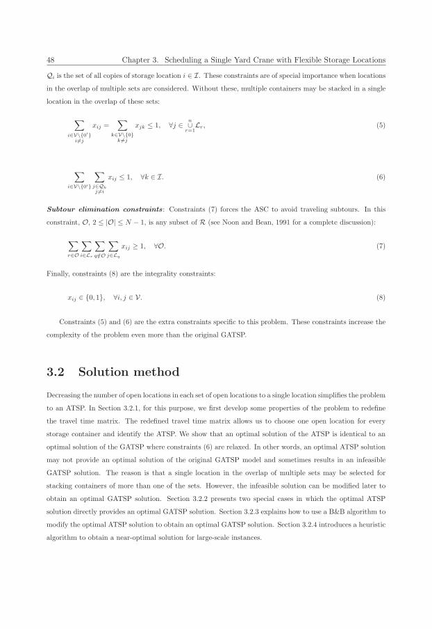
48 Chapter 3. Scheduling a Single Yard Crane with Flexible Storage Locations
Qi is the set of all copies of storage location i ∈ I. These constraints are of special importance when locations
in the overlap of multiple sets are considered. Without these, multiple containers may be stacked in a single
location in the overlap of these sets:
∑i∈V\{0′}
i�=j
xij =∑
k∈V\{0}k �=j
xjk ≤ 1, ∀j ∈ n∪r=1Lr, (5)
∑i∈V\{0′}
∑j∈Qkj �=i
xij ≤ 1, ∀k ∈ I. (6)
Subtour elimination constraints: Constraints (7) forces the ASC to avoid traveling subtours. In this
constraint, O, 2 ≤ |O| ≤ N − 1, is any subset of R (see Noon and Bean, 1991 for a complete discussion):
∑r∈O
∑i∈Lr
∑q/∈O
∑j∈Lq
xij ≥ 1, ∀O. (7)
Finally, constraints (8) are the integrality constraints:
xij ∈ {0, 1}, ∀i, j ∈ V. (8)
Constraints (5) and (6) are the extra constraints specific to this problem. These constraints increase the
complexity of the problem even more than the original GATSP.
3.2 Solution method
Decreasing the number of open locations in each set of open locations to a single location simplifies the problem
to an ATSP. In Section 3.2.1, for this purpose, we first develop some properties of the problem to redefine
the travel time matrix. The redefined travel time matrix allows us to choose one open location for every
storage container and identify the ATSP. We show that an optimal solution of the ATSP is identical to an
optimal solution of the GATSP where constraints (6) are relaxed. In other words, an optimal ATSP solution
may not provide an optimal solution of the original GATSP model and sometimes results in an infeasible
GATSP solution. The reason is that a single location in the overlap of multiple sets may be selected for
stacking containers of more than one of the sets. However, the infeasible solution can be modified later to
obtain an optimal GATSP solution. Section 3.2.2 presents two special cases in which the optimal ATSP
solution directly provides an optimal GATSP solution. Section 3.2.3 explains how to use a B&B algorithm to
modify the optimal ATSP solution to obtain an optimal GATSP solution. Section 3.2.4 introduces a heuristic
algorithm to obtain a near-optimal solution for large-scale instances.
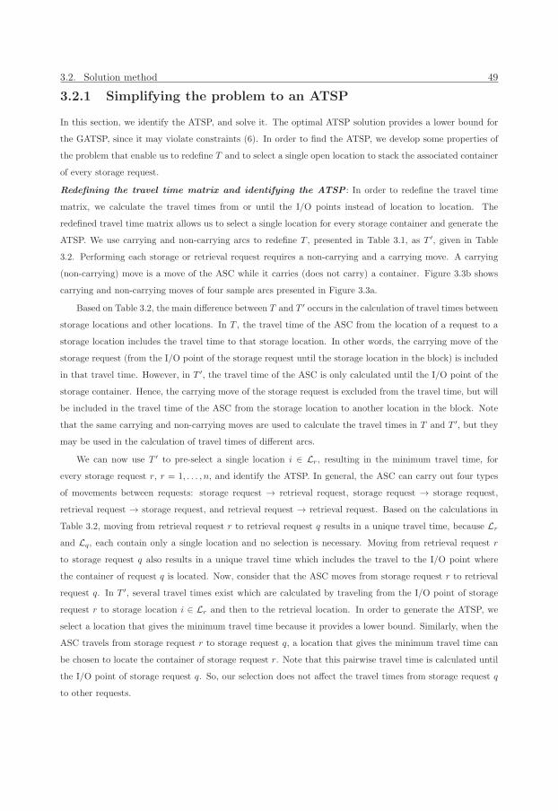
3.2. Solution method 49
3.2.1 Simplifying the problem to an ATSP
In this section, we identify the ATSP, and solve it. The optimal ATSP solution provides a lower bound for
the GATSP, since it may violate constraints (6). In order to find the ATSP, we develop some properties of
the problem that enable us to redefine T and to select a single open location to stack the associated container
of every storage request.
Redefining the travel time matrix and identifying the ATSP : In order to redefine the travel time
matrix, we calculate the travel times from or until the I/O points instead of location to location. The
redefined travel time matrix allows us to select a single location for every storage container and generate the
ATSP. We use carrying and non-carrying arcs to redefine T , presented in Table 3.1, as T ′, given in Table
3.2. Performing each storage or retrieval request requires a non-carrying and a carrying move. A carrying
(non-carrying) move is a move of the ASC while it carries (does not carry) a container. Figure 3.3b shows
carrying and non-carrying moves of four sample arcs presented in Figure 3.3a.
Based on Table 3.2, the main difference between T and T ′ occurs in the calculation of travel times between
storage locations and other locations. In T , the travel time of the ASC from the location of a request to a
storage location includes the travel time to that storage location. In other words, the carrying move of the
storage request (from the I/O point of the storage request until the storage location in the block) is included
in that travel time. However, in T ′, the travel time of the ASC is only calculated until the I/O point of the
storage container. Hence, the carrying move of the storage request is excluded from the travel time, but will
be included in the travel time of the ASC from the storage location to another location in the block. Note
that the same carrying and non-carrying moves are used to calculate the travel times in T and T ′, but they
may be used in the calculation of travel times of different arcs.
We can now use T ′ to pre-select a single location i ∈ Lr, resulting in the minimum travel time, for
every storage request r, r = 1, . . . , n, and identify the ATSP. In general, the ASC can carry out four types
of movements between requests: storage request → retrieval request, storage request → storage request,
retrieval request → storage request, and retrieval request → retrieval request. Based on the calculations in
Table 3.2, moving from retrieval request r to retrieval request q results in a unique travel time, because Lr
and Lq, each contain only a single location and no selection is necessary. Moving from retrieval request r
to storage request q also results in a unique travel time which includes the travel to the I/O point where
the container of request q is located. Now, consider that the ASC moves from storage request r to retrieval
request q. In T ′, several travel times exist which are calculated by traveling from the I/O point of storage
request r to storage location i ∈ Lr and then to the retrieval location. In order to generate the ATSP, we
select a location that gives the minimum travel time because it provides a lower bound. Similarly, when the
ASC travels from storage request r to storage request q, a location that gives the minimum travel time can
be chosen to locate the container of storage request r. Note that this pairwise travel time is calculated until
the I/O point of storage request q. So, our selection does not affect the travel times from storage request q
to other requests.
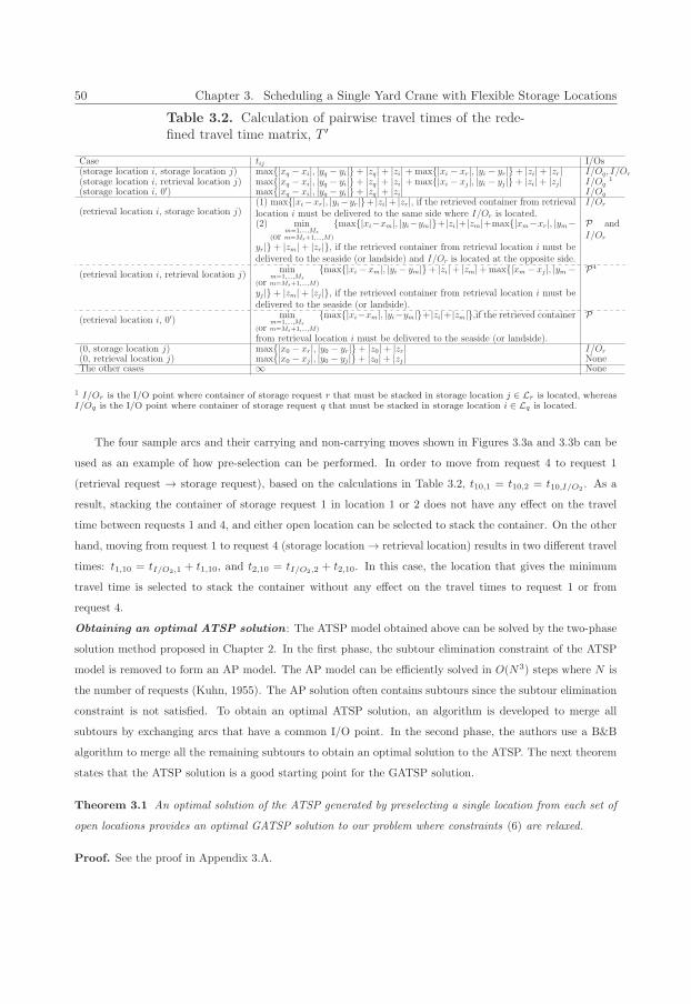
50 Chapter 3. Scheduling a Single Yard Crane with Flexible Storage Locations
Table 3.2. Calculation of pairwise travel times of the rede-fined travel time matrix, T ′
Case tij I/Os(storage location i, storage location j) max{|xq − xi|, |yq − yi|}+ |zq|+ |zi|+max{|xi − xr|, |yi − yr|}+ |zi|+ |zr| I/Oq, I/Or
(storage location i, retrieval location j) max{|xq − xi|, |yq − yi|}+ |zq|+ |zi|+max{|xi − xj|, |yi − yj|}+ |zi|+ |zj| I/Oq1
(storage location i, 0′) max{|xq − xi|, |yq − yi|}+ |zq|+ |zi| I/Oq
(retrieval location i, storage location j)(1) max{|xi−xr|, |yi−yr|}+ |zi|+ |zr|, if the retrieved container from retrievallocation i must be delivered to the same side where I/Or is located.
I/Or
(2) minm=1,...,Ms
(or m=Ms+1,...,M)
{max{|xi−xm|, |yi−ym|}+|zi|+|zm|+max{|xm−xr|, |ym−
yr|}+ |zm|+ |zr|}, if the retrieved container from retrieval location i must bedelivered to the seaside (or landside) and I/Or is located at the opposite side.
P andI/Or
(retrieval location i, retrieval location j)min
m=1,...,Ms
(or m=Ms+1,...,M)
{max{|xi − xm|, |yi − ym|}+ |zi|+ |zm|+max{|xm − xj|, |ym −
yj|}+ |zm|+ |zj|}, if the retrieved container from retrieval location i must bedelivered to the seaside (or landside).
P4
(retrieval location i, 0′) minm=1,...,Ms
(or m=Ms+1,...,M)
{max{|xi−xm|, |yi−ym|}+|zi|+|zm|},if the retrieved container
from retrieval location i must be delivered to the seaside (or landside).
P
(0, storage location j) max{|x0 − xr|, |y0 − yr|}+ |z0|+ |zr| I/Or
(0, retrieval location j) max{|x0 − xj|, |y0 − yj|}+ |z0|+ |zj| NoneThe other cases ∞ None
1 I/Or is the I/O point where container of storage request r that must be stacked in storage location j ∈ Lr is located, whereasI/Oq is the I/O point where container of storage request q that must be stacked in storage location i ∈ Lq is located.
The four sample arcs and their carrying and non-carrying moves shown in Figures 3.3a and 3.3b can be
used as an example of how pre-selection can be performed. In order to move from request 4 to request 1
(retrieval request → storage request), based on the calculations in Table 3.2, t10,1 = t10,2 = t10,I/O2. As a
result, stacking the container of storage request 1 in location 1 or 2 does not have any effect on the travel
time between requests 1 and 4, and either open location can be selected to stack the container. On the other
hand, moving from request 1 to request 4 (storage location→ retrieval location) results in two different travel
times: t1,10 = tI/O2,1 + t1,10, and t2,10 = tI/O2,2 + t2,10. In this case, the location that gives the minimum
travel time is selected to stack the container without any effect on the travel times to request 1 or from
request 4.
Obtaining an optimal ATSP solution : The ATSP model obtained above can be solved by the two-phase
solution method proposed in Chapter 2. In the first phase, the subtour elimination constraint of the ATSP
model is removed to form an AP model. The AP model can be efficiently solved in O(N3) steps where N is
the number of requests (Kuhn, 1955). The AP solution often contains subtours since the subtour elimination
constraint is not satisfied. To obtain an optimal ATSP solution, an algorithm is developed to merge all
subtours by exchanging arcs that have a common I/O point. In the second phase, the authors use a B&B
algorithm to merge all the remaining subtours to obtain an optimal solution to the ATSP. The next theorem
states that the ATSP solution is a good starting point for the GATSP solution.
Theorem 3.1 An optimal solution of the ATSP generated by preselecting a single location from each set of
open locations provides an optimal GATSP solution to our problem where constraints (6) are relaxed.
Proof. See the proof in Appendix 3.A.
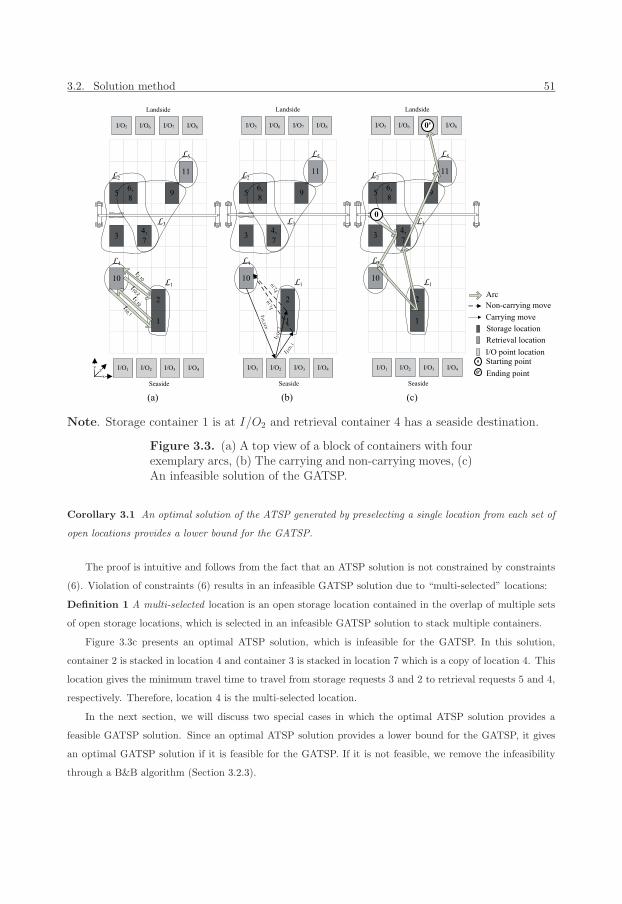
3.2. Solution method 51
Note. Storage container 1 is at I/O2 and retrieval container 4 has a seaside destination.
Figure 3.3. (a) A top view of a block of containers with fourexemplary arcs, (b) The carrying and non-carrying moves, (c)An infeasible solution of the GATSP.
Corollary 3.1 An optimal solution of the ATSP generated by preselecting a single location from each set of
open locations provides a lower bound for the GATSP.
The proof is intuitive and follows from the fact that an ATSP solution is not constrained by constraints
(6). Violation of constraints (6) results in an infeasible GATSP solution due to “multi-selected” locations:
Definition 1 A multi-selected location is an open storage location contained in the overlap of multiple sets
of open storage locations, which is selected in an infeasible GATSP solution to stack multiple containers.
Figure 3.3c presents an optimal ATSP solution, which is infeasible for the GATSP. In this solution,
container 2 is stacked in location 4 and container 3 is stacked in location 7 which is a copy of location 4. This
location gives the minimum travel time to travel from storage requests 3 and 2 to retrieval requests 5 and 4,
respectively. Therefore, location 4 is the multi-selected location.
In the next section, we will discuss two special cases in which the optimal ATSP solution provides a
feasible GATSP solution. Since an optimal ATSP solution provides a lower bound for the GATSP, it gives
an optimal GATSP solution if it is feasible for the GATSP. If it is not feasible, we remove the infeasibility
through a B&B algorithm (Section 3.2.3).
52 Chapter 3. Scheduling a Single Yard Crane with Flexible Storage Locations
3.2.2 Optimal GATSP solution in two special cases
In the following two cases, the optimal ATSP solution provides an optimal GATSP solution.
Case 1: no overlap among every two sets of open locations: Assume sets of open locations do
not overlap. In this case, the optimal ATSP solution cannot contain multi-selected locations, since a multi-
selected location only appears in the overlap of two or more sets. The following theorem states that in this
case an optimal ATSP solution directly provides an optimal GATSP solution:
Theorem 3.2 If sets of open locations of storage requests do not overlap, an optimal ATSP solution is an
optimal GATSP solution.
The proof is intuitive. When sets of open locations do not overlap, no multi-selected location can appear
in the solution. In other words, the optimal ATSP solution satisfies constraints (6), and is thus a feasible
GATSP solution. According to Corollary (3.1), the optimal ATSP solution is an optimal GATSP solution.
Case 2: multi-selected locations can all be replaced by alternative open locations: If sets of open
locations overlap, an optimal ATSP solution may consist of multi-selected locations. In this case, we may still
be able to fix the optimal ATSP solution to obtain an optimal GATSP solution by replacing all multi-selected
locations with other open locations. Because of simultaneous movements of the ASC over the bays and rows
of the block as well as properties of Chebyshev distance, the travel time of the ASC in the horizontal direction
calculated in equation (1) is the maximum travel time in the X and Y directions. As a result, when the ASC
moves from a storage request to another request, multiple open locations may result in the minimum travel
time. We call these locations “alternative open” locations and define them as follows:
Definition 2 Alternative open locations are two or more open locations within a set of open locations which
result in the minimum ASC travel time when used for stacking the storage container followed by traveling to
a next location.
In order to use alternative open locations and remove multi-selected locations, we develop an AP model.
The AP assures that every storage container will be located in a different alternative open location. In this
way, we avoid generating new multi-selected locations while we remove the other ones. The cost matrix of
the AP model is established by using the travel times of the alternative open locations. If a location is an
alternative open location for a storage request, then the cost equals the travel time, otherwise infinity. Note
that the cost matrix includes all storage requests with sets of open locations that overlap with other sets.
These storage requests are either already involved in a multi-selected locations or may result in a multi-
selected location if not included in the AP model. Obviously, storage requests with sets of open locations
which do not overlap with other sets do not cause multi-selected locations. Therefore, they do not need to
be included in the model.
If the AP has an optimal solution less than infinity, a separate alternative open location can be found for
each storage container. Therefore, we can remove all multi-selected locations and obtain an optimal GATSP
solution. Otherwise, the number of alternative open locations is smaller than the number of storage requests,
3.2. Solution method 53
and thus an optimal solution of the GATSP cannot be obtained using the optimal ATSP solution. We then
use the B&B algorithm discussed in Section 3.2.3 to remove the multi-selected locations.
3.2.3 Optimal GATSP solution in the other cases
The input of this section is the optimal ATSP solution which is not a feasible GATSP solution even after using
the alternative open locations algorithm. We develop a B&B algorithm to remove multi-selected locations
and to find a complete tour. The B&B algorithm forbids a single multi-selected location to appear in the
solution, one at a time. This is carried out by keeping and removing locations from sets of open locations in
different nodes. Next, we first explain the main steps of the B&B algorithm, and then present the algorithm.
Branching : We design a branching rule to remove one multi-selected location at a time. The branches divide
the solution space into complementary solution subspaces such that the multi-selected location cannot appear
in any of them. The branching works by keeping the multi-selected location, selected to stack containers of
several sets in the previous solution, in a single set at a time and removing that location from the other ones.
We select the multi-selected location that is in the overlap of more numbers of sets to perform the branching.
Suppose that in a node, the multi-selected location i is in the overlap of U sets of which some have caused
the multi-selected location. The branching rule produces U child nodes. In each child node u ∈ {1, . . . , U},location i appears in only one set and all its copies belonging to Qi are removed from all the other sets. Sets
of open locations that do not contain this specific location remain the same as the parent node.
Bounding and selection of a live node : In section 3.2.2, we solved an ATSP which provides a lower
bound for the GATSP and serves as the input for the B&B algorithm in node 0, if it contains multi-selected
locations. In all the other nodes of the B&B tree, the travel time matrix of the parent node must be
modified first considering the changes in sets of open locations forced by the branching rule, and then an
AP is solved. If an optimal AP objective value is more than the incumbent objective value, the node is
fathomed. Otherwise, alternative open locations and the two-phase solution method proposed in Chapter 2
are consecutively used to remove multi-selected locations and subtours. This method results in a complete
tour but may increase the objective function. Using alternative open locations does not increase the objective
function, but multi-selected locations may still exist in the solution (see Section 3.2.2). As a result, we need to
check for the objective value and multi-selected locations. If the objective value is more than the incumbent
objective value, the node is fathomed; if not, presence of multi-selected locations must be checked. If no
multi-selected location exists, a new incumbent solution is obtained, and the node must be fathomed. If at
least one multi-selected location exists, the node is added to the set of live nodes, E.
Selecting a live node, e, from E is carried out by using the depth-first-search (DFS) as the overall strategy
and the best-first-search (BeFS) when choice is to be made between nodes at the same level of the tree. We
mention this strategy as DFS-BeFS. Clausen (2003) mentions that in the DFS strategy, we select the live
node with the highest level. The level of a specific node in the B&B tree is defined as the number of nodes
between that node and the root node. In the BeFS strategy, the next node to be evaluated is the one with
54 Chapter 3. Scheduling a Single Yard Crane with Flexible Storage Locations
the lowest bound among all the live nodes.
3.2.4 Near-optimal heuristic for large-scale problems
The three-phase solution method can find an optimal GATSP solution. However, the computation time can
be long if the number of requests is large (N ≥ 100). Therefore, instead of solving the problem to optimality,
we use the following heuristic algorithm to quickly find a near-optimal solution. This solution can also serve
as an upper bound for the B&B algorithm.
The heuristic algorithm uses the optimal ATSP solution obtained in Section 3.2.1 and tries to find a
feasible GATSP solution by stacking containers in locations other than the multi-selected locations. Note
that in Section 3.2.2, we have already tried to find alternative open locations and to remove multi-selected
ones. In this algorithm, locations that are chosen are not necessarily alternative open locations, and may
increase the total travel time.
The heuristic algorithm performs very much like the alternative open locations algorithm presented in
Section 3.2.2. It tries to remove multi-selected locations using an AP model. However, in order to establish
the cost matrix of the AP model, instead of the travel times of the alternative open locations, all open
locations of the sets are included. An AP solution results in removing multi-selected locations and obtaining
a feasible GATSP solution with the minimum increase in the total travel time of the ATSP solution. Note
that we always have enough locations to stack all containers; otherwise, the GATSP model does not have a
feasible solution. The gap between the new feasible GATSP solution and the optimal ATSP solution which
is a lower bound to the problem provides a good indicator to evaluate the performance of the heuristic.
3.3 Computational experiments
We conducted multiple numerical experiments to evaluate the performance of the three-phase solution method
and the heuristic algorithm. In each scenario, we consider a single block of containers with 40 or 50 bays,
10 or 20 rows, four tiers, and two, 10, or 20 I/O points. Other inputs regarding the size of containers
and the speed of the ASC can be found in Table 2.2 in Chapter 2. The general data is provided by one
of the largest container terminals in the Port of Rotterdam. The number of storage and retrieval requests
are N = 20, 50, 100, 150 and 200. Their locations and corresponding I/O points are randomly generated by
Monte Carlo simulation. Storage requests have multiple open locations, but the number of potential open
locations per storage request in each scenario is equal and is set to one, four, seven, or 10. All locations are
uniformly distributed over the block, and an equal number of requests have to be picked up or delivered to
the landside and the seaside. The ASC starts its operation from the location of I/O1, and it either ends
at the storage location of a storage request if it is the last request in the sequence, or at an I/O point if a
retrieval request is the last request in the sequence.
3.3. Computational experiments 55
The study is performed on a Notebook with 2.40 GHz Intel� CoreTM i5 processor, with 4.00 GB of
RAM and the programming language is MATLAB� 2010a.
3.3.1 Evaluating the performance of the three-phase solution method
In this section, we evaluate the performance of the three-phase solution method. Table 3.3 shows the results
of the three-phase solution method. The results are categorized into small-scale (20 requests), medium-scale
(50 requests), and large-scale (100 requests) problems. For small-scale and medium-scale problems, 100
realizations are randomly generated for each scenario. Due to the long computation time for large-scale
problems, we randomly generate 20 realizations for each scenario and terminate the computation after 500
seconds. As explained in chapter 2, the number of realizations satisfies Nrealz. ≥ σ2(
(1+ε)Z1−α/2
εμ
)2
with a
90% confidence level (α = 10%), where σ2 and μ are respectively the variance and mean of the objective
values, Z1−α/2 is the 1 − α/2 percentile of the normal distribution, and ε = 5% is for determining the
confidence interval (Law and Kelton, 1999).
The results in Table 3.3 show that the three-phase solution method can quickly obtain the optimal
solution to small-scale (N ≤ 20) and medium-scale (N ≤ 50) problems. Average computation time is less
than 10.45 seconds. Still, by increasing the number of requests, the computation time becomes longer. The
solution to large-scale problems with more than 100 requests cannot be found in a reasonable time. If sets of
open locations have a single member (|Lr| = 1, ∀r ∈ R), we have an ATSP instead of a GATSP. Therefore, the
problem can be solved in less than a second by obtaining an optimal ATSP solution. The first four scenarios
of each problem size in Table 3.3. In addiction, column 11 shows that the minimum number of nodes of the
B&B tree in some realizations is 1. These are the special cases where sets of open locations do not overlap
(case 1 in Section 3.2.2), or alternative open locations can be found (case 2 in Section 3.2.2). The solution
can be obtained rapidly because an optimal ATSP solution directly provides an optimal GATSP solution.
Table 3.4 is used to evaluate how the locations in the set intersections affect the complexity of the problem
and the total travel time of the ASC. We consider an instance with 20 requests in which the number of storage
and retrieval requests is in balance. The number of open locations is also set to 20. Let I be the percentage
of locations that are in the intersection of all sets. The other locations do not belong to any intersection
and are randomly dispatched among all sets. Thus, |Lr| ≥ 20 × I, r = {1, . . . , n}. The results show that
by increasing the number of locations in the set intersections, the computation time significantly grow. On
the other hand, by increasing I, the ASC has more flexibility to stack every container which can be used to
decrease the total travel time.
We also compare the results of 17 randomly selected instances obtained by the three-phase solution
method with those results obtained by CPLEX 12.2. Due to the long computation time of CPLEX to find an
optimal solution of the problem, we truncated the computation after 18000 seconds. The results presented
in Table 3.5 show a large gap between the feasible objective value obtained by CPLEX in 18000 seconds and
the optimal objective value (obtained in less than a second). By increasing the number of requests, the gap
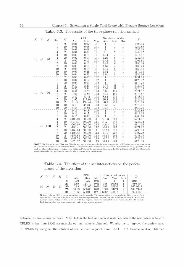
56 Chapter 3. Scheduling a Single Yard Crane with Flexible Storage Locations
Table 3.3. The results of the three-phase solution method
X Y N |Lr| 1 MCPU Number of nodes
Z∗Ave Max Min Ave Max Min
10 40 20
1 2 0.01 0.02 0.01 1 1 1 1303.441 10 0.01 0.08 0.01 1 1 1 1285.891 20 0.01 0.08 0.01 1 1 1 1255.184 2 0.01 0.08 0.01 1.3 7 1 1248.874 10 0.02 0.14 0.01 1.44 7 1 1214.374 20 0.02 0.10 0.01 1.29 8 1 1237.487 2 0.02 0.16 0.01 1.42 9 1 1207.817 10 0.03 0.13 0.01 1.45 6 1 1180.387 20 0.03 0.10 0.01 1.35 4 1 1186.7410 2 0.03 0.13 0.01 1.45 6 1 1180.3810 10 0.03 0.21 0.01 1.52 7 1 1174.1310 20 0.04 0.32 0.01 1.61 8 1 1156.86
10 40 50
1 2 0.03 0.06 0.02 1 1 1 3231.641 10 0.04 0.12 0.02 1 1 1 3126.321 20 0.04 0.63 0.02 1 1 1 3179.744 2 0.30 2.26 0.03 4.79 41 1 3024.504 10 0.35 3.42 0.03 5.56 37 1 2920.334 20 0.41 10.28 0.03 6.01 139 1 2971.377 2 1.84 64.96 0.03 8.46 195 1 2978.877 10 2.42 87.44 0.03 8.62 239 1 2948.987 20 2.97 117.80 0.03 10.8 334 1 2930.6310 2 10.45 198.26 0.03 20.9 293 1 2920.6810 10 3.10 48.34 0.03 6.58 50 1 2875.1110 20 5.54 55.94 0.04 9.37 79 1 2859.76
10 40 100
1 2 0.13 0.18 0.09 1 1 1 6526.891 10 0.12 0.17 0.08 1 1 1 6313.351 20 0.15 0.30 0.09 1 1 1 6266.784 2 >108.60 500.00 0.11 >133 803 1 6271.074 10 >97.59 500.00 0.11 >127 740 1 5736.324 20 >209.69 500.00 0.12 >243 621 1 6114.367 2 >186.41 500.00 0.12 >96.4 307 1 5971.927 10 >169.14 500.00 0.11 >82.4 320 1 5790.947 20 >126.58 500.00 0.13 >71 228 1 6007.7910 2 >157.83 500.00 0.13 >62.5 204 1 6088.7810 10 >241.55 500.00 0.19 >87.6 330 1 5522.1210 20 >223.97 500.00 0.19 >73.7 204 1 6120.98
NOTE. We denote by Ave, Max, and Min the average, maximum and minimum computation (CPU) time and number of nodesof the solution method over 100 realizations. Computation time is calculated in seconds. Furthermore, let |Lr| be the size ofeach set of open locations, r = 1, 2, . . . , n. Column Z∗ shows the average optimal value for the instances with 20 and 50 requestsand it shows the average feasible value for the instances with 100 requests.
Table 3.4. The effect of the set intersections on the perfor-mance of the algorithm
X Y N M ICPU Number of nodes
Z∗Ave Max Min Ave Max Min
10 40 20 10
0 0.02 0.25 0.01 1 1 1 1045.1525 4.89 114.70 0.01 758 16563 1 980.7050 6.85 272.05 0.01 691 24833 1 945.934575 26.38 500.00 0.07 1969 33474 4 944.7448100 151.65 500.00 0.20 6762 24413 5 924.63
Notes. Column CPU is the computation time in seconds. The computation is truncated after 500 seconds. Eachinstance has the same number of retrieval and storage requests. For the last two scenarios, column Z∗ shows theaverage feasible value for the instances with 100 requests since the computation is truncated after 500 seconds.Each instance has the same number of retrieval and storage requests.
between the two values increases. Note that in the first and second instances where the computation time of
CPLEX is less than 18000 seconds the optimal value is obtained. We also try to improve the performance
of CPLEX by using set the solution of our heuristic algorithm and the CPLEX feasible solution obtained
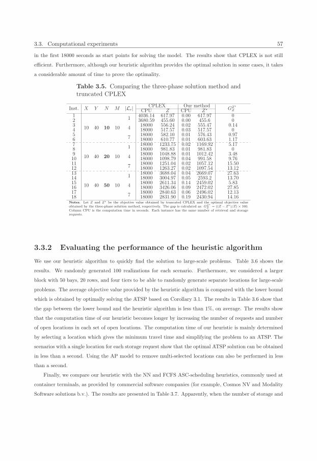
3.3. Computational experiments 57
in the first 18000 seconds as start points for solving the model. The results show that CPLEX is not still
efficient. Furthermore, although our heuristic algorithm provides the optimal solution in some cases, it takes
a considerable amount of time to prove the optimality.
Table 3.5. Comparing the three-phase solution method andtruncated CPLEX
Inst. X Y N M |Lr| CPLEX Our methodGZ∗
ZCPU Z CPU Z∗1
10 40 10 10
14036.14 617.97 0.00 617.97 0
2 3680.59 455.60 0.00 455.6 03
418000 556.24 0.02 555.47 0.14
4 18000 517.57 0.03 517.57 05
718000 582.10 0.01 576.43 0.97
6 18000 610.77 0.01 603.63 1.177
10 40 20 10
118000 1233.75 0.02 1169.92 5.17
8 18000 981.83 0.01 981.83 09
418000 1048.88 0.01 1012.42 3.48
10 18000 1098.79 0.04 991.58 9.7611
718000 1251.04 0.02 1057.12 15.50
12 18000 1263.27 0.02 1097.54 13.1213
10 40 50 10
118000 3688.04 0.04 2669.07 27.63
14 18000 3004.97 0.05 2593.2 13.7015
418000 2611.34 0.14 2459.02 5.83
16 18000 3426.06 0.09 2472.02 27.8517
718000 2840.63 0.06 2496.02 12.13
18 18000 2831.90 0.19 2430.94 14.16Notes. Let Z and Z∗ be the objective value obtained by truncated CPLEX and the optimal objective valueobtained by the three-phase solution method, respectively. The gap is calculated as: GZ∗
Z = ((Z − Z∗)/Z) × 100.Column CPU is the computation time in seconds. Each instance has the same number of retrieval and storagerequests.
3.3.2 Evaluating the performance of the heuristic algorithm
We use our heuristic algorithm to quickly find the solution to large-scale problems. Table 3.6 shows the
results. We randomly generated 100 realizations for each scenario. Furthermore, we considered a larger
block with 50 bays, 20 rows, and four tiers to be able to randomly generate separate locations for large-scale
problems. The average objective value provided by the heuristic algorithm is compared with the lower bound
which is obtained by optimally solving the ATSP based on Corollary 3.1. The results in Table 3.6 show that
the gap between the lower bound and the heuristic algorithm is less than 1%, on average. The results show
that the computation time of our heuristic becomes longer by increasing the number of requests and number
of open locations in each set of open locations. The computation time of our heuristic is mainly determined
by selecting a location which gives the minimum travel time and simplifying the problem to an ATSP. The
scenarios with a single location for each storage request show that the optimal ATSP solution can be obtained
in less than a second. Using the AP model to remove multi-selected locations can also be performed in less
than a second.
Finally, we compare our heuristic with the NN and FCFS ASC-scheduling heuristics, commonly used at
container terminals, as provided by commercial software companies (for example, Cosmos NV and Modality
Software solutions b.v.). The results are presented in Table 3.7. Apparently, when the number of storage and
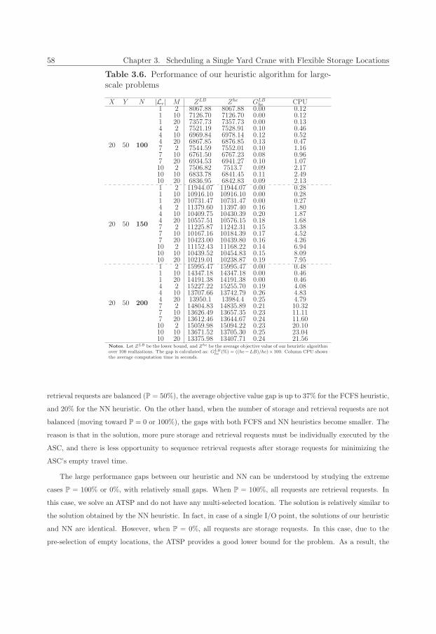
58 Chapter 3. Scheduling a Single Yard Crane with Flexible Storage Locations
Table 3.6. Performance of our heuristic algorithm for large-scale problems
X Y N |Lr| M ZLB Zhe GLBhe CPU
20 50 100
1 2 8067.88 8067.88 0.00 0.121 10 7126.70 7126.70 0.00 0.121 20 7357.73 7357.73 0.00 0.134 2 7521.19 7528.91 0.10 0.464 10 6969.84 6978.14 0.12 0.524 20 6867.85 6876.85 0.13 0.477 2 7544.59 7552.01 0.10 1.167 10 6761.50 6767.23 0.08 0.967 20 6934.53 6941.27 0.10 1.0710 2 7506.82 7513.7 0.09 2.1710 10 6833.78 6841.45 0.11 2.4910 20 6836.95 6842.83 0.09 2.13
20 50 150
1 2 11944.07 11944.07 0.00 0.281 10 10916.10 10916.10 0.00 0.281 20 10731.47 10731.47 0.00 0.274 2 11379.60 11397.40 0.16 1.804 10 10409.75 10430.39 0.20 1.874 20 10557.51 10576.15 0.18 1.687 2 11225.87 11242.31 0.15 3.387 10 10167.16 10184.39 0.17 4.527 20 10423.00 10439.80 0.16 4.2610 2 11152.43 11168.22 0.14 6.9410 10 10439.52 10454.83 0.15 8.0910 20 10219.01 10238.87 0.19 7.95
20 50 200
1 2 15995.47 15995.47 0.00 0.481 10 14347.18 14347.18 0.00 0.461 20 14191.38 14191.38 0.00 0.464 2 15227.22 15255.70 0.19 4.084 10 13707.66 13742.79 0.26 4.834 20 13950.1 13984.4 0.25 4.797 2 14804.83 14835.89 0.21 10.327 10 13626.49 13657.35 0.23 11.117 20 13612.46 13644.67 0.24 11.6010 2 15059.98 15094.22 0.23 20.1010 10 13671.52 13705.30 0.25 23.0410 20 13375.98 13407.71 0.24 21.56
Notes. Let ZLB be the lower bound, and Zhe be the average objective value of our heuristic algorithmover 100 realizations. The gap is calculated as: GLB
he (%) = ((he−LB)/he)×100. Column CPU showsthe average computation time in seconds.
retrieval requests are balanced (P = 50%), the average objective value gap is up to 37% for the FCFS heuristic,
and 20% for the NN heuristic. On the other hand, when the number of storage and retrieval requests are not
balanced (moving toward P = 0 or 100%), the gaps with both FCFS and NN heuristics become smaller. The
reason is that in the solution, more pure storage and retrieval requests must be individually executed by the
ASC, and there is less opportunity to sequence retrieval requests after storage requests for minimizing the
ASC’s empty travel time.
The large performance gaps between our heuristic and NN can be understood by studying the extreme
cases P = 100% or 0%, with relatively small gaps. When P = 100%, all requests are retrieval requests. In
this case, we solve an ATSP and do not have any multi-selected location. The solution is relatively similar to
the solution obtained by the NN heuristic. In fact, in case of a single I/O point, the solutions of our heuristic
and NN are identical. However, when P = 0%, all requests are storage requests. In this case, due to the
pre-selection of empty locations, the ATSP provides a good lower bound for the problem. As a result, the
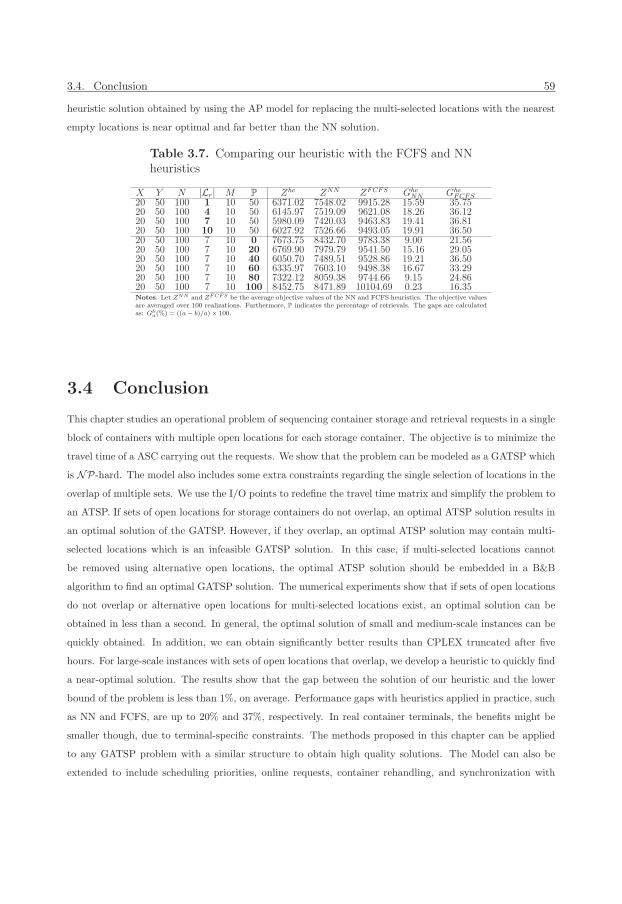
3.4. Conclusion 59
heuristic solution obtained by using the AP model for replacing the multi-selected locations with the nearest
empty locations is near optimal and far better than the NN solution.
Table 3.7. Comparing our heuristic with the FCFS and NNheuristics
X Y N |Lr| M P Zhe ZNN ZFCFS GheNN Ghe
FCFS20 50 100 1 10 50 6371.02 7548.02 9915.28 15.59 35.7520 50 100 4 10 50 6145.97 7519.09 9621.08 18.26 36.1220 50 100 7 10 50 5980.09 7420.03 9463.83 19.41 36.8120 50 100 10 10 50 6027.92 7526.66 9493.05 19.91 36.5020 50 100 7 10 0 7673.75 8432.70 9783.38 9.00 21.5620 50 100 7 10 20 6769.90 7979.79 9541.50 15.16 29.0520 50 100 7 10 40 6050.70 7489.51 9528.86 19.21 36.5020 50 100 7 10 60 6335.97 7603.10 9498.38 16.67 33.2920 50 100 7 10 80 7322.12 8059.38 9744.66 9.15 24.8620 50 100 7 10 100 8452.75 8471.89 10104.69 0.23 16.35Notes. Let ZNN and ZFCFS be the average objective values of the NN and FCFS heuristics. The objective valuesare averaged over 100 realizations. Furthermore, P indicates the percentage of retrievals. The gaps are calculatedas: Gb
a(%) = ((a− b)/a)× 100.
3.4 Conclusion
This chapter studies an operational problem of sequencing container storage and retrieval requests in a single
block of containers with multiple open locations for each storage container. The objective is to minimize the
travel time of a ASC carrying out the requests. We show that the problem can be modeled as a GATSP which
is NP-hard. The model also includes some extra constraints regarding the single selection of locations in the
overlap of multiple sets. We use the I/O points to redefine the travel time matrix and simplify the problem to
an ATSP. If sets of open locations for storage containers do not overlap, an optimal ATSP solution results in
an optimal solution of the GATSP. However, if they overlap, an optimal ATSP solution may contain multi-
selected locations which is an infeasible GATSP solution. In this case, if multi-selected locations cannot
be removed using alternative open locations, the optimal ATSP solution should be embedded in a B&B
algorithm to find an optimal GATSP solution. The numerical experiments show that if sets of open locations
do not overlap or alternative open locations for multi-selected locations exist, an optimal solution can be
obtained in less than a second. In general, the optimal solution of small and medium-scale instances can be
quickly obtained. In addition, we can obtain significantly better results than CPLEX truncated after five
hours. For large-scale instances with sets of open locations that overlap, we develop a heuristic to quickly find
a near-optimal solution. The results show that the gap between the solution of our heuristic and the lower
bound of the problem is less than 1%, on average. Performance gaps with heuristics applied in practice, such
as NN and FCFS, are up to 20% and 37%, respectively. In real container terminals, the benefits might be
smaller though, due to terminal-specific constraints. The methods proposed in this chapter can be applied
to any GATSP problem with a similar structure to obtain high quality solutions. The Model can also be
extended to include scheduling priorities, online requests, container rehandling, and synchronization with

60 Chapter 3. Scheduling a Single Yard Crane with Flexible Storage Locations
other material handling equipment at the terminal.
3.A. Proof of Theorem 3.1 61
Appendix
3.A Proof of Theorem 3.1
Suppose that in an optimal GATSP solution, an open location is chosen that does not give the minimum
time in order to travel from the associated storage request to a next following request. Then, the total travel
time between these two requests can be reduced by replacing this open location with another open location
which gives a shorter travel time. However, replacing all such travel times in the optimal GATSP solution
with minimum travel times results in an optimal solution to the ATSP model in which open locations that
result in the minimum travel time are pre-selected. Of course, this may not be a feasible GATSP solution,
since constraints (6) may be violated and a location in the overlap of multiple sets may be chosen to locate
multiple containers. �

Chapter 4
Scheduling Two Non-Passing Yard
Cranes∗
In this chapter, we study an extension of chapter 2 and 3 where we minimize the makespan of the two
non-passing automated stacking cranes (ASCs) carrying out a set of storage and retrieval requests in a block
of containers. In addition to determining the order in which to carry out the requests, we determine a
location for each storage request under the following operational constraints. When a container is to be
retrieved to the seaside, the seaside ASC picks it up from its location in the block and drops it at the seaside
input/output (I/O) point. When a storage request is to be stacked from the seaside, the seaside ASC picks
it up and stores it in a location in the block, selected from a set of available open locations specified for that
request. Each open storage location can be occupied by at most one container. Landside operations can be
carried out similarly. The ASCs can carry out single cycle or double cycle movements to carry out requests.
In a single cycle movement, the ASC carries out a single storage or retrieval request and returns to the I/O
point to carry out another request, whereas in a double cycle, the ASC combines a storage request with a
retrieval request in order to reduce the empty travel time (Goodchild and Daganzo, 2006, 2007). The ASCs
can never pass each other and must operate sufficiently far from each other. Since the ASCs cannot pass
each other, seaside requests are carried out by the seaside ASC and landside requests are carried out by the
landside ASC. Containers should not be dropped off in any location other than their final locations since this
requires additional ASC movements which are time-consuming. We consider different priorities in stacking
or retrieving containers. The most important reasons for this are as follows:
� The performance of a container terminal is often evaluated based on the berthing times of ships (Bose,
2011). Therefore, seaside containers usually have a higher priority than landside containers.
� To ensure the stability of ships, heavy containers must be loaded before light containers, in lower tiers
∗This chapter is based on Gharehgozli et al. (2012a).
63
64 Chapter 4. Scheduling Two Non-Passing Yard Cranes
on the ship and must therefore be retrieved earlier (see, for example, Chapter 5, Kim et al., 2000,
Sammarra et al., 2007, Dekker et al., 2007).
� Trucks, trains and ships arrive at a container yard to deliver or pick up containers in different time
windows (see, for example, Froyland et al., 2008, Petering, 2011b, Newman and Yano, 2000), which
induces precedence constraints on the stacking and retrieving of containers.
Preventing reshuffles also imposes additional precedence constraints on the operations. A reshuffle is an
unwanted movement of a container stacked on top of another one that has to be retrieved (Kim et al., 2000,
De Castillo and Daganzo, 1993, Caserta and Voß, 2009). For example, a precedence constraint can prohibit
a container to be stacked in a pile before retrieving a container located in the same pile, or it can force
containers stacked on top of a specific container to be retrieved earlier.
We formulate this multi-crane problem as a multiple asymmetric generalized traveling salesman problem
with precedence constraints (mAGTSP-PC), which generalizes the single version of the problem without such
constraints (see, for example, Laporte et al., 1987, Noon and Bean, 1991). The model also contains additional
constraints regarding the interactions of the ASCs and the selection of open storage locations which lie in
the intersection of multiple sets. We will elaborate on these constraints in the problem description section.
We develop an adaptive large neighborhood search heuristic for this problem.
Our scientific contribution is to develop and solve a continuous time model to schedule two interacting
ASCs working in a single block of containers. Our model incorporates precedence constraints, ASC interac-
tion constraints, and constraints that assign each container to a storage location selected from a given set.
Considering these constraints is valuable not only from a theoretical standpoint but also from a practical
point of view. In practice, containers have different priorities, and a set of suitable open locations is available
for each container that has to be stacked. The mAGTSP and its variants have been shown to be NP-hard(see, for example, Cheung et al., 2002, Narasimhan and Palekar, 2002) and the new features introduced in
this study make the problem even more difficult to solve.
The remainder of this chapter is organized as follows. In Section 4.1, we describe the technical aspects of
the problem and present our mathematical model. Section 4.2 describes the heuristic. Section 4.3 presents
numerical results, and Section 4.4 contains the conclusions.
4.1 Problem description and model
This section describes the research problem, introduces notations, and then formulates the problem as an
mAGTSP-PC.
4.1. Problem description and model 65
4.1.1 Problem description
We seek to determine the sequence to stack containers of n storage requests and retrieve containers of N −n
retrieval requests in a single block of containers consisting of X rows, Y bays, Z tiers and two I/O points,
one at each end of the block. We denote by S and L the seaside and landside I/O points, respectively. Let
R be the set of all requests, whereas Rs and Rl be the sets of requests that must be picked up or dropped
off at S and L, respectively.
The objective is to minimize the makespan of the two ASCs carrying out these requests. We denote
by ASCs the seaside ASC assigned to Rs, and by ASCl the landside ASC assigned to Rl. Each ASC can
carry only one container at a time. From a given starting point, each ASC can execute its requests in any
sequence in order to minimize its total travel time. We denote by 0s and 0′s, respectively, the starting and
ending locations of ASCs, whereas 0l and 0′l are the corresponding locations for ASCl. These locations can
be anywhere in the block. The ASCs cannot pass each other and have to be be separated by a distance
taking τ time units to travel. The storage and retrieval containers can be of different sizes (20 or 40 feet)
and leave or arrive at the container terminal by truck, train or ship. Containers should not be dropped off
at temporary locations. Finally, the speed of an empty or full ASC is the same.
Every storage or retrieval request r ∈ R = {1, . . . , N} corresponds to a unique container. For storage
request r, an ASC moves a container from the I/O point where it is located to a location i in the block
selected from a given set Lr of available open locations. For retrieval request r, an ASC moves a container
from location j in the block to a specified I/O point. For ease of notation, we write that the location j of
retrieval request r belongs to Lr. Thus, the set V of all locations can be defined as:
V = {1, 2, . . . , |L1|︸ ︷︷ ︸L1
, |L1|+ 1, |L1|+ 2, . . . , |L1|+ |L2|︸ ︷︷ ︸L2
, . . . ,n−1∑i=1
|Li|+ 1,n−1∑i=1
|Li|+ 2, . . . ,n∑
i=1
|Li|︸ ︷︷ ︸Ln
,
n∑i=1
|Li|+ 1
︸ ︷︷ ︸Ln+1
, . . . ,
n∑i=1
|Li|+N − n
︸ ︷︷ ︸LN
, 0s︸︷︷︸L0s
, 0l︸︷︷︸L0l
, 0′s︸︷︷︸L0′s
, 0′l︸︷︷︸L0′
l
}.
For each storage location in V lying in the intersection of multiple sets, a copy is created for each set
to which it belongs. The copy locations will be used in the model to avoid stacking multiple containers in
the same location. The same as the previous two chapters, we assume that storage and retrieval locations as
well as destination sides of retrieval containers and I/O points of storage containers are known; in practice,
they are determined at a higher hierarchical planning level. This level focuses on minimizing the number of
reshufflings (De Castillo and Daganzo, 1993, Kim et al., 2000) and speeding up the loading and unloading
process of a ship (Kim and Kim, 1999a, Vis and Roodbergen, 2009). Furthermore, due to the abundance of
internal transport vehicles (like AGVs and chassis) to pick up containers at the seaside and landside, retrieved
containers can be delivered to any I/O point at each side. Because of the same reason, retrieval containers
can be quickly moved away from all I/O points, and they can therefore be delivered to the same I/O point
that a storage container has to be picked up. The other issue is that storage and retrieval locations do not
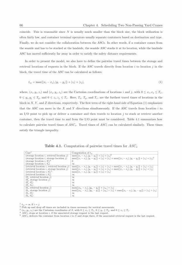
66 Chapter 4. Scheduling Two Non-Passing Yard Cranes
coincide. This is reasonable since N is usually much smaller than the block size, the block utilization is
often fairly low, and container terminal operators usually separate containers based on destination and type.
Finally, we do not consider the collaboration between the ASCs. In other words, if a container comes from
the seaside and has to be stacked at the landside, the seaside ASC stacks it at its location, while the landside
ASC has moved sufficiently far away in order to satisfy the safety distance requirements.
In order to present the model, we also have to define the pairwise travel times between the storage and
retrieval locations of requests in the block. If the ASC travels directly from location i to location j in the
block, the travel time of the ASC can be calculated as follows:
tij = max{|xi − xj |, |yi − yj |}+ |zi|+ |zj |, (1)
where, (xi, yi, zi) and (xj , yj , zj) are the Cartesian coordinations of locations i and j, with 0 ≤ xi, xj ≤ Tx,
0 ≤ yi, yj ≤ Ty, and 0 ≤ zi, zj ≤ Tz. Here, Tx, Ty, and Tz, are the furthest travel times of locations in the
block in X, Y , and Z directions, respectively. The first term of the right-hand side of Equation (1) emphasizes
that the ASC can move in the X and Y directions simultaneously. If the ASC travels from location i to
an I/O point to pick up or deliver a container and then travels to location j to stack or retrieve another
container, then the travel time to and from the I/O point must be considered. Table 4.1 summarizes how
to calculate pairwise travel times of ASCs. Travel times of ASCl can be calculated similarly. These times
satisfy the triangle inequality.
Table 4.1. Computation of pairwise travel times for ASCs
Case1 Computation of tij(storage location i, retrieval location j) max{|xi − xj|, |yi − yj|}+ |zi|+ |zj|2(storage location i, storage location j) max{|xi − xs|, |yi − ys|}+ |zi|+ |zs|+max{|xs − xj|, |ys − yj|}+ |zs|+ |zj|3(storage location i, 0′s)
4 0(storage location i, 0s) ∞(retrieval location i, retrieval location j) max{|xi − xs|, |yi − ys|}+ |zi|+ |zs|+max{|xs − xj|, |ys − yj|}+ |zs|+ |zj|(retrieval location i, storage location j) max{|xi − xs|, |yi − ys|}+ |zi|+ |zs|+max{|xs − xj|, |ys − yj|}+ |zs|+ |zj|(retrieval location i, 0′s)
5 max{|xi − xs|, |yi − ys|}+ |zi|+ |zs|(retrieval location i, 0s) ∞(0′s, retrieval location j) ∞(0′s, storage location j) ∞(0′s, 0
′s) ∞
(0′s, 0s) ∞(0s, retrieval location j) max{|x0s − xj|, |y0s − yj|}+ |z0s |+ |zj|(0s, storage location j) max{|x0s − xs|, |y0s − ys|}+ |z0s |+ |zs|+max{|xs − xj|, |ys − yj|}+ |zs|+ |zj|(0s, 0
′s) ∞
(0s, 0s) ∞
1 tij = ∞ if i = j.2 Pick up and drop off times are included in times necessary for vertical movements.3 (xs, ys, zs) are the Cartesian coordinates of S, with 0 ≤ xs ≤ Tx, 0 ≤ ys ≤ Ty , and 0 ≤ zs ≤ Tz .4 ASCs stops at location i, if the associated storage request is the last request.5 ASCs delivers the container from location i to S and stops there, if the associated retrieval request is the last request.
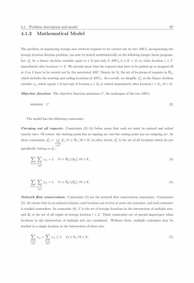
4.1. Problem description and model 67
4.1.2 Mathematical Model
The problem of sequencing storage and retrieval requests to be carried out by two ASCs, incorporating the
storage location decision problem, can now be stated mathematically as the following integer linear program.
Let xkij be a binary decision variable equal to 1 if and only if ASCk, k ∈ K = {l, s} visits location j ∈ V
immediately after location i ∈ V. We already know that the requests that have to be picked up or dropped off
at S or L have to be carried out by the associated ASC. Denote by Vk the set of locations of requests in Rk,
which includes the starting and ending locations of ASCk. As a result, we simplify xkij as the binary decision
variable xij which equals 1 if and only if location j ∈ Vk is visited immediately after location i ∈ Vk, ∀k ∈ K.
Objective function : The objective function minimizes C, the makespan of the two ASCs:
minimize C (2)
The model has the following constraints.
Carrying out all requests : Constraints (3)–(4) below mean that each set must be entered and exited
exactly once. Of course, the starting point has no ingoing arc and the ending point has no outgoing arc. In
these constraints, L′r =
⋃e∈Rke�=r
Le, ∀r ∈ Rk, ∀k ∈ K; in other words, L′r is the set of all locations which do not
specifically belong to Lr:
∑i∈L′
r
∑j∈Lrj �=i
xij = 1, ∀r ∈ Rk\{0k}, ∀k ∈ K, (3)
∑i∈Lr
∑j∈L′
rj �=i
xij = 1, ∀r ∈ Rk\{0′k}, ∀k ∈ K. (4)
Network flow conservation : Constraints (5) are the network flow conservation constraints. Constraints
(5)–(6) ensure that in an optimal solution, each location can receive at most one container, and each container
is stacked somewhere. In constraint (6), I is the set of storage locations in the intersection of multiple sets,
and Qi is the set of all copies of storage location i ∈ I. These constraints are of special importance when
locations in the intersection of multiple sets are considered. Without these, multiple containers may be
stacked in a single location in the intersection of these sets:
∑i∈Vki�=j
xij =∑l∈Vkl �=j
xjl ≤ 1, ∀j ∈ Vk, ∀k ∈ K, (5)
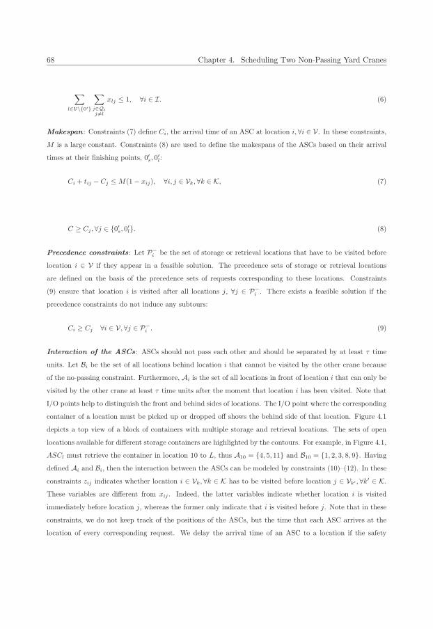
68 Chapter 4. Scheduling Two Non-Passing Yard Cranes
∑l∈V\{0′}
∑j∈Qij �=l
xlj ≤ 1, ∀i ∈ I. (6)
Makespan : Constraints (7) define Ci, the arrival time of an ASC at location i, ∀i ∈ V. In these constraints,
M is a large constant. Constraints (8) are used to define the makespans of the ASCs based on their arrival
times at their finishing points, 0′s, 0′l:
Ci + tij − Cj ≤M(1− xij), ∀i, j ∈ Vk, ∀k ∈ K, (7)
C ≥ Cj , ∀j ∈ {0′s, 0′l}. (8)
Precedence constraints: Let P−i be the set of storage or retrieval locations that have to be visited before
location i ∈ V if they appear in a feasible solution. The precedence sets of storage or retrieval locations
are defined on the basis of the precedence sets of requests corresponding to these locations. Constraints
(9) ensure that location i is visited after all locations j, ∀j ∈ P−i . There exists a feasible solution if the
precedence constraints do not induce any subtours:
Ci ≥ Cj ∀i ∈ V, ∀j ∈ P−i . (9)
Interaction of the ASCs: ASCs should not pass each other and should be separated by at least τ time
units. Let Bi be the set of all locations behind location i that cannot be visited by the other crane because
of the no-passing constraint. Furthermore, Ai is the set of all locations in front of location i that can only be
visited by the other crane at least τ time units after the moment that location i has been visited. Note that
I/O points help to distinguish the front and behind sides of locations. The I/O point where the corresponding
container of a location must be picked up or dropped off shows the behind side of that location. Figure 4.1
depicts a top view of a block of containers with multiple storage and retrieval locations. The sets of open
locations available for different storage containers are highlighted by the contours. For example, in Figure 4.1,
ASCl must retrieve the container in location 10 to L, thus A10 = {4, 5, 11} and B10 = {1, 2, 3, 8, 9}. Havingdefined Ai and Bi, then the interaction between the ASCs can be modeled by constraints (10)–(12). In these
constraints zij indicates whether location i ∈ Vk, ∀k ∈ K has to be visited before location j ∈ Vk′ , ∀k′ ∈ K.These variables are different from xij . Indeed, the latter variables indicate whether location i is visited
immediately before location j, whereas the former only indicate that i is visited before j. Note that in these
constraints, we do not keep track of the positions of the ASCs, but the time that each ASC arrives at the
location of every corresponding request. We delay the arrival time of an ASC to a location if the safety
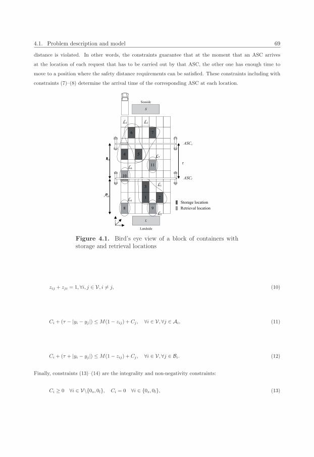
4.1. Problem description and model 69
distance is violated. In other words, the constraints guarantee that at the moment that an ASC arrives
at the location of each request that has to be carried out by that ASC, the other one has enough time to
move to a position where the safety distance requirements can be satisfied. These constraints including with
constraints (7)–(8) determine the arrival time of the corresponding ASC at each location.
Figure 4.1. Bird’s eye view of a block of containers withstorage and retrieval locations
zij + zji = 1, ∀i, j ∈ V, i �= j, (10)
Ci + (τ − |yi − yj |) ≤M(1− zij) + Cj , ∀i ∈ V, ∀j ∈ Ai, (11)
Ci + (τ + |yi − yj |) ≤M(1− zij) + Cj , ∀i ∈ V, ∀j ∈ Bi. (12)
Finally, constraints (13)–(14) are the integrality and non-negativity constraints:
Ci ≥ 0 ∀i ∈ V\{0s, 0l}, Ci = 0 ∀i ∈ {0s, 0l}, (13)
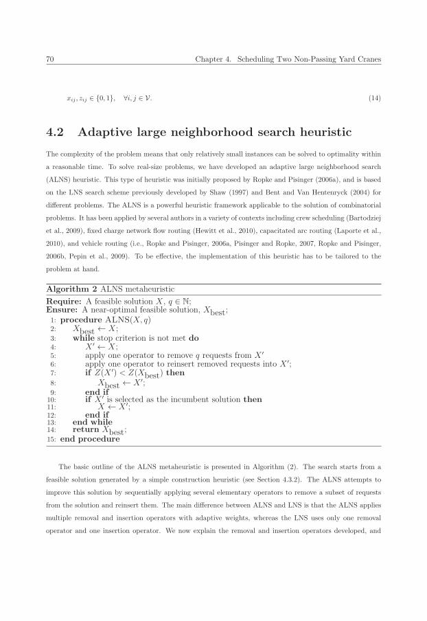
70 Chapter 4. Scheduling Two Non-Passing Yard Cranes
xij , zij ∈ {0, 1}, ∀i, j ∈ V. (14)
4.2 Adaptive large neighborhood search heuristic
The complexity of the problem means that only relatively small instances can be solved to optimality within
a reasonable time. To solve real-size problems, we have developed an adaptive large neighborhood search
(ALNS) heuristic. This type of heuristic was initially proposed by Ropke and Pisinger (2006a), and is based
on the LNS search scheme previously developed by Shaw (1997) and Bent and Van Hentenryck (2004) for
different problems. The ALNS is a powerful heuristic framework applicable to the solution of combinatorial
problems. It has been applied by several authors in a variety of contexts including crew scheduling (Bartodziej
et al., 2009), fixed charge network flow routing (Hewitt et al., 2010), capacitated arc routing (Laporte et al.,
2010), and vehicle routing (i.e., Ropke and Pisinger, 2006a, Pisinger and Ropke, 2007, Ropke and Pisinger,
2006b, Pepin et al., 2009). To be effective, the implementation of this heuristic has to be tailored to the
problem at hand.
Algorithm 2 ALNS metaheuristic
Require: A feasible solution X, q ∈ N;Ensure: A near-optimal feasible solution, Xbest;1: procedure ALNS(X, q)2: Xbest ← X;3: while stop criterion is not met do4: X ′ ← X;5: apply one operator to remove q requests from X ′6: apply one operator to reinsert removed requests into X ′;7: if Z(X ′) < Z(Xbest) then8: Xbest ← X ′;9: end if10: if X ′ is selected as the incumbent solution then11: X ← X ′;12: end if13: end while14: return Xbest;15: end procedure
The basic outline of the ALNS metaheuristic is presented in Algorithm (2). The search starts from a
feasible solution generated by a simple construction heuristic (see Section 4.3.2). The ALNS attempts to
improve this solution by sequentially applying several elementary operators to remove a subset of requests
from the solution and reinsert them. The main difference between ALNS and LNS is that the ALNS applies
multiple removal and insertion operators with adaptive weights, whereas the LNS uses only one removal
operator and one insertion operator. We now explain the removal and insertion operators developed, and
4.2. Adaptive large neighborhood search heuristic 71
then in Section 4.2.3, we describe how to update and use the weights to select a removal and an insertion
operator in each iteration.
4.2.1 Removal operators
We have developed several removal operators, all of which are applied to a feasible solution. Note that in
this problem, one of the ASCs needs to visit a unique location for each request. In our operators, we refer to
corresponding requests of locations.
Relatedness removal (Shaw removal): The Shaw operator, initially introduced by Shaw (1997), is one
of the most widely used removal operators. It removes the requests which are somewhat related to each
other and can be inserted interchangeably in different positions of the solution. In our implementation, the
relatedness of requests r and e is defined as:
R(r, e) = ϕ|typer − typee|+ χ|sider − sidee|+ ψ||Pr| − |Pe||+ ω|vr − ve|, (15)
where, typer equals 1 if request r is a storage request, and 0 otherwise; sider equals 1 if request r has to be
picked up or dropped of at S, and 0 otherwise; Pr is the set of requests that must appear either before or after
request r; and vr is the location associated with request r. In order to apply equation (15), all variables are
scaled to take values between 0 and 1. The smaller R(r, e) is, the more related r and e are. The complexity
of this operator is O(N).
Random removal : In this type of removal, q requests are randomly removed from the solution. The
complexity of this operator is O(1) and it is repeated q times.
Worst removal : Assume that Δ(r,X) is the travel time of request r to its predecessor and successor
requests in the solution. The worst removal operator removes q requests with the largest Δ(r,X). Note that
we do not define Δ(r,X) as the effect of removing request r in the objective function. Indeed, because of
the interactions between the ASCs, and because of the precedence constraints, fully evaluating the objective
function for each partial solution is rather time consuming. Our simplified approach avoids this computation.
The complexity of this operator stems from the sorting process involved in the operator which is O(N2).
Precedence constraint removal : This operator sorts the requests of the solution in non-decreasing order
of |Pr|, and then selects the first q requests. The rationale is that since these requests have smaller number
of predecessors and successors, their reinsertion in the solution is likely to be easier. The complexity of this
operator is O(N2).
Group removal : In the group removal operator, either q storage requests or q retrieval requests are removed
from the solution. The idea is that storage or retrieval requests can be used to generate double cycles when
72 Chapter 4. Scheduling Two Non-Passing Yard Cranes
they are reinserted in the solution. In our implementation, we choose the first q storage or retrieval requests
in the solution. However, one may remove those with the largest Δ(r,X) or |Pr|. The complexity of this
operator is O(N) and it is repeated q times.
Single cycle removal : This operator removes q single cycles from the current solution. It is expected that
better double cycles than the current ones in terms of the objective function can be generated by reinserting
their requests in the solution. In this operator, as in the group removal operator, we remove the first q
single cycles, but one can alternatively remove those with the largest Δ(r,X) or |Pr|. If there is no single
cycle location, the random removal operator removes requests until a new single cycle can be found. The
complexity of this operator is O(N) and it is repeated q times.
Location removal : One of the features of our problem is the presence of sets of open locations to stack
storage containers. In the heuristic used to generate a feasible initial solution, the location for each storage
container is randomly selected from its set of available open locations. If no operator is applied to assign new
locations, the selected locations do not change, which results in lost opportunities to improve the solution. The
location removal operator, randomly selects max{n, q} storage requests and removes the locations assigned
to them. A location insertion operator then selects other locations for these requests (see the next section).
The complexity of this operator is O(N) and it is repeated max{n, q} times.
4.2.2 Insertion operators
We have developed four operators to reinsert the q requests that have been removed by one of the above
operators. The insertion operators regain solution feasibility, by sequencing all requests, while satisfying the
precedence and interaction constraints.
Greedy reinsertion : Let Δfr be the travel time of request r to its predecessor and successor request by
inserting it in its best position. The greedy operator inserts the request minimizing Δfr, over all removed
requests. After inserting a request, the operator updates the Δfr values and is reapplied. The complexity of
this operator is O(N) and it is repeated q times.
Random reinsertion : This operator randomly reinserts the requests into the partial solution. The com-
plexity of this operator is O(1) and it is repeated q times.
Interaction insertion : The main idea of this operator is to insert seaside and landside requests in the
partial solution so as to minimize the interaction of the corresponding ASCs. When a request is inserted in
a position, the operator counts the immediate requests after and before the request that have to be delivered
to the same side. It then inserts the request in a position yielding the largest number. The complexity of
this operator is O(N) and it is repeated q times.
4.2. Adaptive large neighborhood search heuristic 73
Location insertion : The location removal operator described in Section 4.2.1 can only be followed by the
location insertion operator. For each storage request with a removed location, this operator randomly selects
a new location from its set of available open locations. The complexity of this operator is O(1) and it is
repeated max{n, q} times.
4.2.3 Choosing a removal operator or a insertion operator
We run the ALNS algorithm for a preset number of iterations. At each iteration, the selection of a removal
or insertion operator is governed by a roulette-wheel mechanism which selects operator o from the set of
removal or insertion operators with probability wo/∑O
o′=1 wo′ , where wo is the weight of operator o, and O
is the number of operators of the set.
In the ALNS, an initial weight is assigned to each operator and the weights are then updated after every
δ iterations of the algorithm. The updates are based on the score that each operator has gained during
the past δ iterations. At each iteration, the score of each operator is updated based on its performance:
the weight of each removal or insertion operator used in the current iteration is incremented by σ1 if their
application result in a new best solution; by σ2 if result in a better incumbent solution; and by σ3 if result
in a solution which is not better than the best solution found and incumbent solution but is accepted, where
σ1 ≥ σ2 ≥ σ3. Let πo and θo be the total score of operator o and the number of times it has been selected after
δ iterations, respectively. Furthermore, let ζo ≥ 1 be a normalization factor which reflects the computational
effort that operator o requires (see Ropke and Pisinger, 2006b). The weight of operator o is then updated
as wo ← wo(1 − ρ) + ρπo/ζoθo, where ρ ∈ [0, 1] is the reaction factor which controls how quickly the weight
adjustment reacts to changes in the operator performance. Note that wo does not change if θo = 0.
4.2.4 Acceptance of the new solution and stop criterion
In order to produce sufficient diversification in the search process, the ALNS metaheuristic is executed
within a simulated annealing (SA) framework (Kirkpatrick et al., 1983), which has proven to work well for
the solution of several combinatorial problems (e.g., Vis and Carlo, 2010, Bozer and Carlo, 2008, Wilhelm
and Ward, 1987). In the SA framework, if the solution found at the current iteration is better than the
current solution, it is accepted. Otherwise, it is accepted with probability e−(Z(S′)−Z(S∗))/T , where T is
the temperature, Z(S′) and Z(S∗) are the objective values of the solution at the current iteration and best
solution, respectively. The temperature starts at Tstart and is updated at each iteration as T ← Tφ, where
0 < φ < 1 is a cooling rate.
74 Chapter 4. Scheduling Two Non-Passing Yard Cranes
4.3 Computational experiments
Extensive numerical experiments were performed to assess the effectiveness of our ALNS metaheuristic. In
Section 4.3.1, we discuss how its parameters were tuned. Section 4.3.2 compares the results of the ALNS
with those results of the LNS, truncated CPLEX, and some other simple heuristics.
The ALNS and the other heuristics were coded in C++ using Microsoft Visual Studio 2008 and were
executed on a Notebook with 2.40 GHz Intel� CoreTM i5 processor, with 4.00 GB of RAM. Exact results
were obtained by CPLEX 12.2 coded in C++ using the Concert Technology framework and executed by
a g++ compiler on a 2.40 GHz AMD OpteronTM Processor 250, with 8.00 GB of RAM under the Linux
operating system.
4.3.1 Tuning and initial solution
In our experiments, we consider a single block of containers with 40 bays, 10 rows, and four tiers. The
number N of requests is set to 10, 25 and 45, which is approximately the workload of a single ASC without
any interaction in a common 40 to 180 minute planning horizon (Vis and Carlo, 2010). We assume an equal
number of open locations |Lr| for storage requests r = 1, . . . , n, and we set |Lr| equal to 1, 3, or 5. As a
result we perform nine basic experiments, numbered as one to nine, on five randomly generated instances in
each case. Each instance has the same number of retrieval and storage requests. All locations are uniformly
distributed over the block, and an equal number of requests have to be picked up or delivered to the landside
and the seaside. The landside ASC starts its operations from L and ends either at the storage position of a
storage request if this is the last request in the sequence, or at L if a retrieval request is the last request in
the sequence. Similarly, the seaside ASC starts from S and either finishes in a storage position or at S.
We assume that the containers are categorized in five priority levels of decreasing importance. In addition,
we consider a sixth priority level dedicated to containers that can be moved at any time. Since the seaside
process time of a terminal has a relatively higher importance, the seaside containers have to be moved before
the other ones, which gives them the priority levels 1, 2, and 3. Eighty percent of remaining containers are
categorized with the priority levels 4 to 6 and 20% with the priority levels 1 to 3. Other inputs regarding the
size of containers and the speed of the ASC can be found in Table 2.2 in Chapter 2.
We have used the first instance of Experiment 5 with 25 requests and three open locations for each storage
requests to tune the parameters of the ALNS. As Ropke and Pisinger (2006a) suggest, we have applied an
ad hoc trial and error strategy to set the parameters. To this end, we have fixed all parameters and changed
only one parameter at a time. The ALNS was applied five times and the parameter value resulting in the best
objective was selected. The parameters used for all scenarios are as follows: (ϕ, χ, ψ, ω, σ1, σ2, σ3, ρ, φ, δ) =
(4, 2, 3, 6, 33, 13, 9, 0.2, 0.94, 200). In our implementation, we have used ζo = 1 for all removal and insertion
operators except for the single cycle and worst removal where ζo = 5. We set the number of ALNS iterations to
25000. The insertion or removal operators have equal weights at the first iteration. The starting temperature
4.3. Computational experiments 75
of the SA was set in such a way that a solution 30% worse than the initial solution should be accepted
with probability 0.5. In the first third of all scenarios, the number of q requests to be removed and inserted
was randomly drawn from the interval [1, 0.5N ], using a semi-triangular distributions with a negative slope.
The interval was narrowed down to [1, 0.25N ] and [1, 0.1N ] for the second and third tiers of the iterations,
respectively.
4.3.2 Computational results
The results obtained by the ALNS are now compared with those results obtained by truncated CPLEX and
with other heuristics.
Comparing ALNS and truncated CPLEX
Tables 4.2, 4.3, and 4.4 compare the makespan and computation time of the ALNS and truncated CPLEX
over different instances. For each instance, we apply the ALNS 20 times each with a different random
initial solution and calculate the minimum, average, and maximum makespan, in addition to the average
computation time. The CPLEX algorithm is applied to each instance only once in order to find a solution
for the mAGTSP-PC and mAGTSP which is a relaxed problem without the precedence constraints and the
ASC interaction constraints. The computation time of CPLEX for finding an optimal or even a feasible
solution for the mAGTSP-PC is very high and we therefore truncate the computation after 14400 seconds.
On the other hand, the mAGTSP can be quickly solved. The reason is that when |Lr| = 1, r = 1, . . . , n,
by relaxing the precedence and ASC constraints we can easily find an optimal solution of the mAGTSP
by solving an assignment problem (AP). Since there is only a single I/O point for each ASC, by using it
all subtours obtained by the AP can be easily merged. When |Lr| > 1, r = 1, . . . , n, the situation is more
complicated since we have to choose a location for each storage container. However, since the number of
requests is relatively small in our instances, we can quickly find the optimal solution with CPLEX. The
optimal mAGTSP solution value provides a lower bound for the original problem.
Table 4.2 compares the optimal results obtained by CPLEX with the ALNS results for small instances.
Column GZAve shows that the ALNS objective values are on average within 0.34% of the optimal values. On
the other hand, as column GLBZ shows, even on small-size instances, the gap between the lower bound and
the optimal mAGTSP-PC solution is large. The gap stems from the fact that the precedence constraints and
interaction constraints significantly affect the sequence of requests carried out by the ASCs and increase the
objective function. Omitting these constraints results in a relaxed problem whose optimal solution provides
a very poor lower bound for the original problem. This suggests that although the gap between the average
ALNS solution value and the lower bound may be large in some cases, this does not necessarily reflect on the
quality of the ALNS algorithm. Therefore, column GAveLB which shows the gap between the lower bound and
average ALNS solution is omitted from the table. A fair assessment is to compare the average result of the
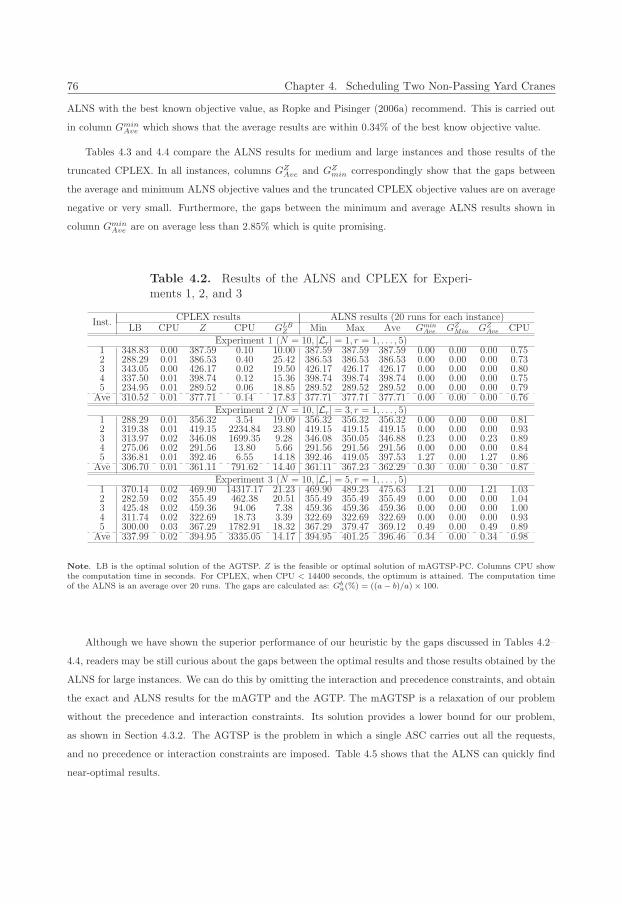
76 Chapter 4. Scheduling Two Non-Passing Yard Cranes
ALNS with the best known objective value, as Ropke and Pisinger (2006a) recommend. This is carried out
in column GminAve which shows that the average results are within 0.34% of the best know objective value.
Tables 4.3 and 4.4 compare the ALNS results for medium and large instances and those results of the
truncated CPLEX. In all instances, columns GZAve and GZ
min correspondingly show that the gaps between
the average and minimum ALNS objective values and the truncated CPLEX objective values are on average
negative or very small. Furthermore, the gaps between the minimum and average ALNS results shown in
column GminAve are on average less than 2.85% which is quite promising.
Table 4.2. Results of the ALNS and CPLEX for Experi-ments 1, 2, and 3
Inst.CPLEX results ALNS results (20 runs for each instance)
LB CPU Z CPU GLBZ Min Max Ave Gmin
Ave GZMin GZ
Ave CPU
Experiment 1 (N = 10, |Lr| = 1, r = 1, . . . , 5)1 348.83 0.00 387.59 0.10 10.00 387.59 387.59 387.59 0.00 0.00 0.00 0.752 288.29 0.01 386.53 0.40 25.42 386.53 386.53 386.53 0.00 0.00 0.00 0.733 343.05 0.00 426.17 0.02 19.50 426.17 426.17 426.17 0.00 0.00 0.00 0.804 337.50 0.01 398.74 0.12 15.36 398.74 398.74 398.74 0.00 0.00 0.00 0.755 234.95 0.01 289.52 0.06 18.85 289.52 289.52 289.52 0.00 0.00 0.00 0.79
Ave 310.52 0.01 377.71 0.14 17.83 377.71 377.71 377.71 0.00 0.00 0.00 0.76
Experiment 2 (N = 10, |Lr| = 3, r = 1, . . . , 5)1 288.29 0.01 356.32 3.54 19.09 356.32 356.32 356.32 0.00 0.00 0.00 0.812 319.38 0.01 419.15 2234.84 23.80 419.15 419.15 419.15 0.00 0.00 0.00 0.933 313.97 0.02 346.08 1699.35 9.28 346.08 350.05 346.88 0.23 0.00 0.23 0.894 275.06 0.02 291.56 13.80 5.66 291.56 291.56 291.56 0.00 0.00 0.00 0.845 336.81 0.01 392.46 6.55 14.18 392.46 419.05 397.53 1.27 0.00 1.27 0.86
Ave 306.70 0.01 361.11 791.62 14.40 361.11 367.23 362.29 0.30 0.00 0.30 0.87
Experiment 3 (N = 10, |Lr| = 5, r = 1, . . . , 5)1 370.14 0.02 469.90 14317.17 21.23 469.90 489.23 475.63 1.21 0.00 1.21 1.032 282.59 0.02 355.49 462.38 20.51 355.49 355.49 355.49 0.00 0.00 0.00 1.043 425.48 0.02 459.36 94.06 7.38 459.36 459.36 459.36 0.00 0.00 0.00 1.004 311.74 0.02 322.69 18.73 3.39 322.69 322.69 322.69 0.00 0.00 0.00 0.935 300.00 0.03 367.29 1782.91 18.32 367.29 379.47 369.12 0.49 0.00 0.49 0.89
Ave 337.99 0.02 394.95 3335.05 14.17 394.95 401.25 396.46 0.34 0.00 0.34 0.98
Note. LB is the optimal solution of the AGTSP. Z is the feasible or optimal solution of mAGTSP-PC. Columns CPU showthe computation time in seconds. For CPLEX, when CPU < 14400 seconds, the optimum is attained. The computation timeof the ALNS is an average over 20 runs. The gaps are calculated as: Gb
a(%) = ((a− b)/a)× 100.
Although we have shown the superior performance of our heuristic by the gaps discussed in Tables 4.2–
4.4, readers may be still curious about the gaps between the optimal results and those results obtained by the
ALNS for large instances. We can do this by omitting the interaction and precedence constraints, and obtain
the exact and ALNS results for the mAGTP and the AGTP. The mAGTSP is a relaxation of our problem
without the precedence and interaction constraints. Its solution provides a lower bound for our problem,
as shown in Section 4.3.2. The AGTSP is the problem in which a single ASC carries out all the requests,
and no precedence or interaction constraints are imposed. Table 4.5 shows that the ALNS can quickly find
near-optimal results.
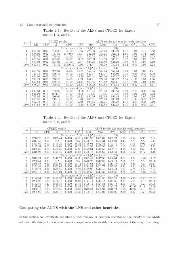
4.3. Computational experiments 77
Table 4.3. Results of the ALNS and CPLEX for Experi-ments 4, 5, and 6
Inst.CPLEX results ALNS results (20 runs for each instance)
LB CPU Z CPU GLBZ Min Max Ave Gmin
Ave GZMin GZ
Ave CPU
Experiment 4 (N = 25, |Lr| = 1, r = 1, . . . , 13)1 660.26 0.02 728.36 14400 9.35 728.36 756.00 739.19 1.47 0.00 0.11 3.502 608.06 0.02 747.62 11730.83 18.67 747.62 789.15 761.44 1.81 0.00 0.14 3.263 733.75 0.02 749.54 14400 2.11 749.54 776.57 758.57 1.19 0.00 0.09 3.354 675.55 0.01 805.03 14400 16.08 805.03 812.33 806.77 0.22 0.00 0.02 2.975 809.92 0.02 827.04 14400 2.07 826.78 854.89 834.26 0.90 -0.03 0.07 3.12
Ave 697.51 0.02 771.52 13866.17 9.66 771.47 797.79 780.05 1.12 -0.01 0.09 3.24
Experiment 5 (N = 25, |Lr| = 3, r = 1, . . . , 13)1 653.96 0.07 952.04 14400 31.31 952.04 952.04 952.04 0.00 0.00 0.00 4.412 715.18 0.06 846.43 14400 15.51 842.57 849.37 845.80 0.38 -0.46 -0.01 4.423 624.06 0.06 869.14 14400 28.20 869.14 906.20 885.17 1.81 0.00 0.16 4.094 738.29 0.06 776.28 14400 4.89 767.41 824.80 809.12 5.15 -1.16 0.33 4.965 659.84 0.06 860.45 14400 23.31 860.45 870.99 863.61 0.37 0.00 0.03 4.66
Ave 678.27 0.06 860.87 14400 20.64 858.32 880.68 871.15 1.54 -0.32 0.10 4.51
Experiment 6 (N = 25, |Lr| = 5, r = 1, . . . , 13)1 618.33 0.16 763.93 14400 19.06 713.34 773.40 733.86 2.80 -7.09 -0.30 5.062 641.96 0.15 1071.37 14400 40.08 1071.37 1071.37 1071.37 0.00 0.00 0.00 5.723 706.86 0.16 886.09 14400 20.23 886.09 920.08 893.48 0.83 0.00 0.07 6.194 688.31 0.16 715.19 14400 3.76 705.01 725.63 708.63 0.51 -1.44 -0.07 4.775 667.79 0.15 721.13 14400 7.40 693.15 722.71 703.08 1.41 -4.04 -0.18 5.10
Ave 664.65 0.16 831.54 14400 18.10 813.79 842.64 822.08 1.11 -2.51 -0.09 5.37
Table 4.4. Results of the ALNS and CPLEX for Experi-ments 7, 8, and 9
Inst.CPLEX results ALNS results (20 runs for each instance)
LB CPU Z CPU GLBZ Min Max Ave Gmin
Ave GZMin GZ
Ave CPU
Experiment 7 (N = 45, |Lr| = 1, r = 1, . . . , 23)1 1240.20 0.03 1326.44 14400 6.50 1321.95 1367.07 1339.21 1.29 -0.34 0.95 12.642 1341.59 0.03 NA 14400 NA 1406.13 1503.34 1456.24 3.44 NA NA 11.443 1451.60 0.03 1775.20 14400 18.23 1778.04 1832.83 1791.75 0.77 0.16 0.92 11.984 1187.91 0.03 1418.68 14400 16.27 1401.92 1447.53 1425.19 1.63 -1.20 0.46 13.225 1368.85 0.03 1461.50 14400 6.34 1422.84 1542.50 1469.79 3.19 -2.72 0.56 13.00
Ave 1318.03 0.03 1495.46 14400 11.83 1466.18 1538.65 1496.44 2.06 -1.02 0.72 12.46
Experiment 8 (N = 45, |Lr| = 3, r = 1, . . . , 23)1 1313.27 0.31 1441.71 14400 8.91 1392.42 1477.36 1436.01 3.04 -3.54 -0.40 19.072 1250.54 0.31 NA 14400 NA 1516.23 1610.82 1556.11 2.56 NA NA 20.303 1260.58 0.30 1597.99 14400 21.11 1464.64 1583.35 1511.18 3.08 -9.10 -5.74 20.444 1132.84 0.30 1392.69 14400 18.66 1284.52 1401.77 1335.53 3.82 -8.42 -4.28 14.305 1178.74 0.30 1515.75 14400 22.23 1439.96 1513.48 1465.41 1.74 -5.26 -3.44 17.64
Ave 1227.19 0.30 1487.04 14400 17.73 1419.55 1517.36 1460.85 2.85 -6.58 -3.46 18.35
Experiment 9 (N = 45, |Lr| = 5, r = 1, . . . , 23)1 1188.81 1.26 1468.33 14400 19.04 1350.82 1424.86 1395.43 3.20 -8.70 -5.22 27.312 1203.28 1.28 1486.10 14400 19.03 1414.11 1515.43 1444.65 2.11 -5.09 -2.87 28.563 1162.50 1.27 1519.36 14400 23.49 1406.12 1524.84 1443.78 2.61 -8.05 -5.23 27.084 1120.03 1.27 1433.51 14400 21.87 1262.19 1333.39 1285.71 1.83 -13.57 -11.50 22.305 1370.13 1.28 1788.55 14400 23.39 1612.51 1686.91 1640.71 1.72 -10.92 -9.01 28.37
Ave 1208.95 1.27 1539.17 14400 21.36 1409.15 1497.09 1442.06 2.29 -9.27 -6.77 26.72
Comparing the ALNS with the LNS and other heuristics
In this section, we investigate the effect of each removal or insertion operator on the quality of the ALNS
solution. We also perform several numerical experiments to identify the advantages of the adaptive strategy
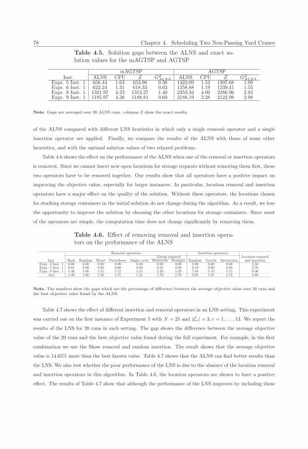
78 Chapter 4. Scheduling Two Non-Passing Yard Cranes
Table 4.5. Solution gaps between the ALNS and exact so-lution values for the mAGTSP and AGTSP
mAGTSP AGTSPInst. ALNS CPU Z GZ
ALNS ALNS CPU Z GZALNS
Expr. 5 Inst. 1 656.44 1.63 653.96 0.38 1322.09 1.52 1307.68 1.09Expr. 6 Inst. 1 622.24 1.31 618.33 0.63 1258.88 1.19 1239.41 1.55Expr. 8 Inst. 1 1331.97 4.23 1313.27 1.40 2353.34 4.00 2286.96 2.82Expr. 9 Inst. 1 1195.97 4.38 1188.81 0.60 2188.19 3.28 2122.98 2.98
Note. Gaps are averaged over 20 ALNS runs. columns Z show the exact results.
of the ALNS compared with different LNS heuristics in which only a single removal operator and a single
insertion operator are applied. Finally, we compare the results of the ALNS with those of some other
heuristics, and with the optimal solution values of two relaxed problems.
Table 4.6 shows the effect on the performance of the ALNS when one of the removal or insertion operators
is removed. Since we cannot insert new open locations for storage requests without removing them first, these
two operators have to be removed together. Our results show that all operators have a positive impact on
improving the objective value, especially for larger instances. In particular, location removal and insertion
operators have a major effect on the quality of the solution. Without these operators, the locations chosen
for stacking storage containers in the initial solution do not change during the algorithm. As a result, we lose
the opportunity to improve the solution by choosing the other locations for storage containers. Since most
of the operators are simple, the computation time does not change significantly by removing them.
Table 4.6. Effect of removing removal and insertion opera-tors on the performance of the ALNS
Removal operators Insertion operatorsGroup removal Location removal
Inst. Shaw Random Worst Precedence Single cycle Retrievals Storages Random Greedy Interaction and insertionExpr. 2 Inst. 1 0.00 0.00 0.00 0.00 0.00 0.00 0.00 3.90 0.00 0.00 3.58Expr. 5 Inst. 1 0.01 0.00 0.00 0.00 0.00 0.01 0.00 0.19 0.00 0.00 2.76Expr. 8 Inst. 1 4.46 4.98 4.51 5.12 4.54 5.26 5.29 7.64 5.43 5.15 8.06
Ave 1.49 1.66 1.50 1.71 1.51 1.76 1.76 3.91 1.81 1.72 4.80
Note. The numbers show the gaps which are the percentage of difference between the average objective value over 20 runs andthe best objective value found by the ALNS.
Table 4.7 shows the effect of different insertion and removal operators in an LNS setting. This experiment
was carried out on the first instance of Experiment 5 with N = 25 and |Lr| = 3, r = 1, . . . , 13. We report the
results of the LNS for 20 runs in each setting. The gap shows the difference between the average objective
value of the 20 runs and the best objective value found during the full experiment. For example, in the first
combination we use the Shaw removal and random insertion. The result shows that the average objective
value is 14.65% more than the best known value. Table 4.7 shows that the ALNS can find better results than
the LNS. We also test whether the poor performance of the LNS is due to the absence of the location removal
and insertion operators in this algorithm. In Table 4.6, the location operators are shown to have a positive
effect. The results of Table 4.7 show that although the performance of the LNS improves by including these
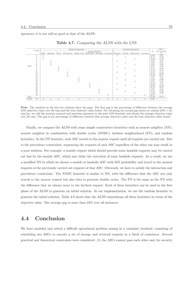
4.4. Conclusion 79
operators, it is not still as good as that of the ALNS.
Table 4.7. Comparing the ALNS with the LNS
Comb.Removal operators Insertion operators
GLNS +
group removal loc rem/insShaw Random Worst Precedence Single cycle Retrievals Storages Location Random Greedy Interaction Location G
LNS
1 � � 14.65 9.972 � � 21.18 16.963 � � 18.86 14.494 � � 3.43 0.015 � � 8.09 2.956 � � 2.92 0.497 � � 6.13 4.638 � � 15.11 10.249 � � 11.32 9.1910 � � 11.55 11.2111 � � 23.29 22.5812 � � 19.42 16.1113 � � 4.21 1.5614 � � 13.28 10.9615 � � 8.72 5.9516 � � 11.02 7.8217 � � 18.85 16.4818 � � 20.70 18.6719 � � 7.99 6.2420 � � 19.19 14.4221 � � 14.63 13.3822 � � 22.07
Ave 13.48 10.74ALNS 23 � � � � � � � � � � � � 0.00
Note. The numbers in the last two columns show the gaps. The first gap is the percentage of difference between the averageLNS objective value over 20 runs and the best objective value found. For obtaining the second gap shown in column LNS + locrem/ins, we add the location removal and insertion operators to the pure LNS heuristic and obtain the average objective valueover 20 runs. The gap is the percentage of difference between this average objective value and the best objective value found.
Finally, we compare the ALNS with some simple constructive heuristics such as nearest neighbor (NN),
nearest neighbor in combination with double cycles (NNDC), farthest neighborhood (FN), and random
heuristics. In the NN heuristic, each ASC travels to the nearest request until all requests are carried out. Due
to the precedence constraints, sequencing the requests of each ASC regardless of the other one may result in
a poor solution. For example, a seaside request which should precede some landside requests may be carried
out last by the seaside ASC, which may delay the execution of some landside requests. As a result, we use
a modified NN in which we choose a seaside or landside ASC with 50% probability and travel to the nearest
requests of the previously carried out requests of that ASC. Obviously, we have to satisfy the interaction and
precedence constraints. The NNDC heuristic is similar to NN, with the difference that the ASC not only
travels to the nearest request but also tries to generate double cycles. The FN is the same as the NN with
the difference that we always move to the farthest request. Each of these heuristics can be used in the first
phase of the ALNS to generate an initial solution. In our implementation, we use the random heuristic to
generate the initial solution. Table 4.8 shows that the ALNS outperforms all these heuristics in terms of the
objective value. The average gap is more than 24% over all instances.
4.4 Conclusion
We have modeled and solved a difficult operational problem arising in a container terminal, consisting of
scheduling two ASCs to execute a set of storage and retrieval requests in a block of containers. Several
practical and theoretical constraints were considered: (1) the ASCs cannot pass each other and, for security
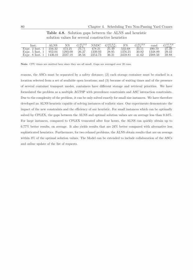
80 Chapter 4. Scheduling Two Non-Passing Yard Cranes
Table 4.8. Solution gaps between the ALNS and heuristicsolution values for several constructive heuristics
Inst. ALNS NN GALNSNN NNDC GALNS
NNDC FN GALNSFN rand GALNS
randExpr. 2 Inst. 1 356.32 473.25 24.71 478.21 25.49 532.68 33.11 490.70 27.39Expr. 5 Inst. 1 952.04 1293.09 26.37 1339.93 28.95 1376.21 30.82 1348.89 29.42Expr. 8 Inst. 1 1436.01 2337.18 38.56 2254.73 36.31 2459.81 41.62 2388.56 39.88
Note. CPU times are omitted here since they are all small. Gaps are averaged over 20 runs.
reasons, the ASCs must be separated by a safety distance; (2) each storage container must be stacked in a
location selected from a set of available open locations; and (3) because of waiting times and of the presence
of several container transport modes, containers have different storage and retrieval priorities. We have
formulated the problem as a multiple AGTSP with precedence constraints and ASC interaction constraints.
Due to the complexity of the problem, it can be only solved exactly for small size instances. We have therefore
developed an ALNS heuristic capable of solving instances of realistic sizes. Our experiments demonstrate the
impact of the new constraints and the efficiency of our heuristic. For small instances which can be optimally
solved by CPLEX, the gaps between the ALNS and optimal solution values are on average less than 0.34%.
For large instances, compared to CPLEX truncated after four hours, the ALNS can quickly obtain up to
6.77% better results, on average. It also yields results that are 24% better compared with alternative less
sophisticated heuristics. Furthermore, for two relaxed problems, the ALNS obtain results that are on average
within 3% of the optimal solution values. The Model can be extended to include collaboration of the ASCs
and online update of the list of requests.
Chapter 5
Minimizing the Expected Number of
Reshuffles ∗
As a result of the exponential container handling growth in the last decades, containers should be stacked
multi-high at container terminals, using handling equipment like straddle carriers, rubber-tired gantry (RTG)
cranes, or rail-mounted gantry (RMG) cranes. Stacking containers multi-high often leads to reshuffling. A
reshuffle is the removal of a container stacked on top of a desired container. Containers are commonly stacked
in sequence of their arrivals which can conflict with the retrieval sequence required by the ships’ stowage plans.
This results in a number of reshuffles. Containers of a ship are usually classified into different classes based
on their weights and ports of destination. In order to ensure the ship’s stability, heavier containers should be
stacked in lower tiers of a ship. In addition, containers of ports of destination that will be visited by the ship
later should be loaded onto the ship earlier. It is therefore beneficial if containers are stacked in a reverse
sequence in every pile of the block. Moreover, if containers of multiple ships and ports of destination are
mixed in a pile, a container leaving earlier should be stacked at a higher tier in order to avoid reshuffling.
It is rather difficult, or even impossible, to control the arrival sequence of containers at the terminal, as
many containers arrive one by one by individual trucks or by internal transport trucks from rail or barge
terminals. Therefore, they should be stacked onto piles as they arrive, which makes later reshuffling inevitable.
Since reshuffling is time consuming and increases berthing times of ships, reducing the number of reshuffles,
while retrieving containers, is a top concern for stacking containers (Kim, 1997, Zhao and Goodchild, 2010).
We study how to stack incoming containers in a container block with the objective of minimizing the
expected number of reshuffles. We develop a heuristic algorithm to quickly find near-optimal solutions for
large-scale problems with a realistic block size (expressed in number of piles). Our heuristic algorithm uses the
results of a stochastic dynamic programming (DP) model built on work of Kim et al. (2000). We show that
∗This chapter is based on Gharehgozli et al. (2012c).
81
82 Chapter 5. Minimizing the Expected Number of Reshuffles
the total number of states of the DP model increases exponentially in the dimensions of the block and types
of containers. It follows that optimal solution of only small-scale problems can be obtained in a reasonable
time. Therefore, we develop the heuristic algorithm in a way that the solution of large-scale problems can be
quickly obtained. The algorithm maps all the states of the DP model for small-scale problems onto decision
trees which help to recognize the correlation between the decisions made by the DP model for different states
of the block. We are then able to simplify and generalize the trees into generalized decision trees using these
similarities. The simplification and generalization significantly reduce the complexity of the trees compared
to the original ones. As a result, the generalized trees can quickly locate incoming containers in a block with
a real number of piles. We can always improve the decisions made by the generalized trees as long as DP
results of larger-scale problems are available. The numerical experiments show that the decisions can be made
in less than a second. The decisions are optimal for small-scale and near-optimal for large scale problems.
The results obtained by the proposed heuristic are significantly better than the results obtained by stacking
policies commonly used in practice. Using these trees, we also study the effect of a shared-stacking (SS)
policy on reducing the expected number of reshuffles. An SS policy allows containers of multiple ships to be
stacked on top of each other in a pile. This differs from a dedicated-stacking (DS) policy, where containers
of a single ship cannot be mixed in a pile. Finally, the decision trees can be used to determine the storage
locations in the models developed in the previous three chapters.
The decision tree (DT) heuristic is novel and differs from the one proposed by Kim et al. (2000) in
several aspects. (1) Our method uses the DP results differently as our method maps all the states of DP
solutions in the decision trees as nodes and branches and then simplifies and generalizes them, while Kim
et al. (2000) use “machine learning logic” which produces the branches of decision trees one by one based
on the amount of information each branch will provide for making decision on where to locate an incoming
container. (2) Our heuristic can optimally solve small-scale problems. Furthermore, it can quickly find the
solution of large-scale problems with a realistic number of piles that cannot be solved by the DP while Kim
et al. (2000) solve problems up to six piles only. The quality of their solution even in case of six piles depends
on the CV P . (3) Our decision trees are open for further improvements; when a larger problem is solved by
the DP, our decision trees can be extended to include the new information provided by the DP and more
accurately solve larger problems. Kim et al. (2000) need to rerun the algorithm to find new decision trees as
their trees are not open to extension.
The rest of this chapter is organized as follows. In Section 5.1, we formulate a stochastic DP model to
locate incoming containers. In Section 5.2, a heuristic solution algorithm is developed. Section 5.3 presents
numerical results. Finally, in Section 5.4, we conclude the chapter and present possible future research topics.
5.1. Problem description and model 83
5.1 Problem description and model
This section describes the research problem, introduces notations, and then formulates the problem as a
stochastic DP model.
5.1.1 Problem description and notations
We study how to stack containers in a single container block by minimizing the expected number of reshuffles.
We use the following notations and assumptions.
� Containers are of the same size (i.e. 20 feet) and are to be loaded onto S ships. Let Qs be the total
number of containers belonging to ship s = 1, 2, . . . , S, and Q =∑S
s=1 Qs.
� In Section 1, we explained that to maintain the weight stability of a ship, heavier containers of that ship
should be loaded onto lower tiers of the ship. Furthermore, ports of destination of containers should
be taken into consideration when they are loaded onto the ship. Finally, we study a problem where
containers of multiple ships can be stacked on top of each other in each pile of the block. Obviously,
containers should be loaded onto the ships in the sequence of the departure of their corresponding
ships.
In order to satisfy the constraints mentioned above, we define C as the set of all types of incoming
containers. Containers of type c must be retrieved earlier than containers of type c + 1, ∀c ∈ C.
Containers of the same type can be retrieved in any order. The size of the set of all container types
depends on the number of ships, number of weight groups and the number of ports of destination.
Assume that ws and ds are the numbers of weight groups and ports of destination of ship s, s =
1, 2, . . . , S. Then, |C| = ∑Ss=1(ws × ds) is the cardinality of C.
� Containers arrive at the container block individually and randomly and they are stored in the block
based on a first-come-first-served (FCFS) sequence. The probability P(c) of receiving a container
of type c ∈ C is a function of its weight group, port of destination and the size of the corre-
sponding ship. We assume uniform probabilities of receiving a container of type c of ship s, or
P(c) = Qs∑Sj=1(wj×dj)×
∑Si=1 Qi
. Obviously,∑
c∈C P(c) = 1. The probabilities do not change by receiving
containers.
� Each pile can be shared by containers of different ships up to T tiers. We distinguish the type of a
pile, Pct, according to the type of its first-leaving container (not necessarily the topmost container),
and the number of open slots available above the upmost container, t, 1 ≤ t ≤ T − 1. Pile types with
t = 0 and T are denoted as PF (full pile) and PE (empty pile), respectively.
� The block has B bays, R rows and T tiers. The total number of piles, V = B × R. Let Vct,
VF and VE denote the numbers of pile types Pct, PF and PE , respectively. Then, we have V =∑c∈C
∑T−1t=1 Vct + VF + VE .
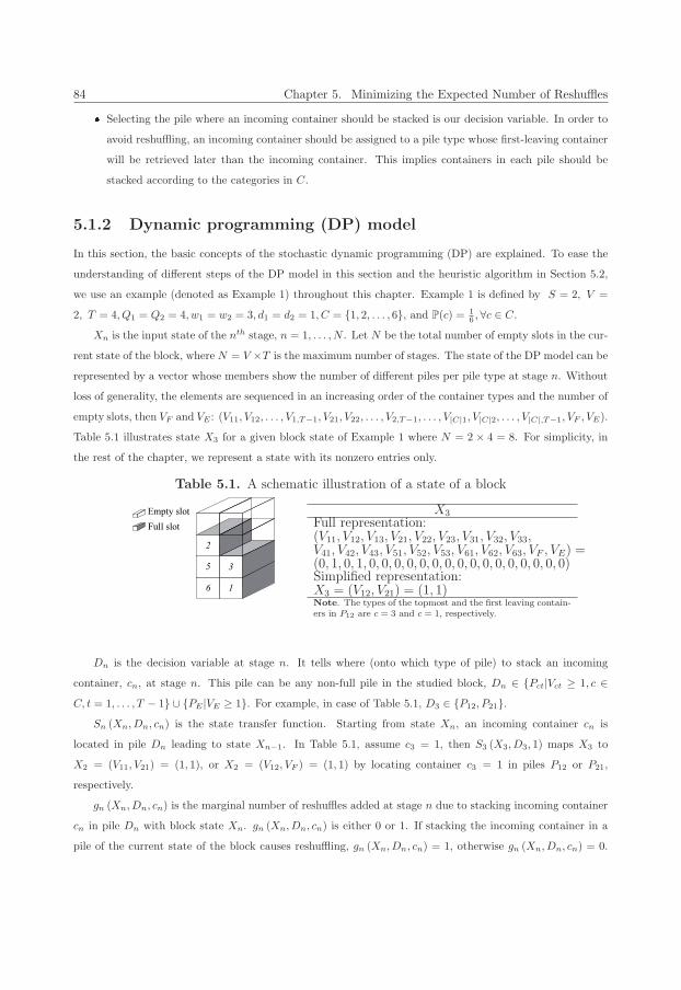
84 Chapter 5. Minimizing the Expected Number of Reshuffles
� Selecting the pile where an incoming container should be stacked is our decision variable. In order to
avoid reshuffling, an incoming container should be assigned to a pile type whose first-leaving container
will be retrieved later than the incoming container. This implies containers in each pile should be
stacked according to the categories in C.
5.1.2 Dynamic programming (DP) model
In this section, the basic concepts of the stochastic dynamic programming (DP) are explained. To ease the
understanding of different steps of the DP model in this section and the heuristic algorithm in Section 5.2,
we use an example (denoted as Example 1) throughout this chapter. Example 1 is defined by S = 2, V =
2, T = 4, Q1 = Q2 = 4, w1 = w2 = 3, d1 = d2 = 1, C = {1, 2, . . . , 6}, and P(c) = 16 , ∀c ∈ C.
Xn is the input state of the nth stage, n = 1, . . . , N . Let N be the total number of empty slots in the cur-
rent state of the block, where N = V ×T is the maximum number of stages. The state of the DP model can be
represented by a vector whose members show the number of different piles per pile type at stage n. Without
loss of generality, the elements are sequenced in an increasing order of the container types and the number of
empty slots, then VF and VE : (V11, V12, . . . , V1,T−1, V21, V22, . . . , V2,T−1, . . . , V|C|1, V|C|2, . . . , V|C|,T−1, VF , VE).
Table 5.1 illustrates state X3 for a given block state of Example 1 where N = 2 × 4 = 8. For simplicity, in
the rest of the chapter, we represent a state with its nonzero entries only.
Table 5.1. A schematic illustration of a state of a block
X3Full representation:(V11, V12, V13, V21, V22, V23, V31, V32, V33,V41, V42, V43, V51, V52, V53, V61, V62, V63, VF , VE) =(0, 1, 0, 1, 0, 0, 0, 0, 0, 0, 0, 0, 0, 0, 0, 0, 0, 0, 0, 0)Simplified representation:X3 = (V12, V21) = (1, 1)Note. The types of the topmost and the first leaving contain-ers in P12 are c = 3 and c = 1, respectively.
Dn is the decision variable at stage n. It tells where (onto which type of pile) to stack an incoming
container, cn, at stage n. This pile can be any non-full pile in the studied block, Dn ∈ {Pct|Vct ≥ 1, c ∈C, t = 1, . . . , T − 1} ∪ {PE |VE ≥ 1}. For example, in case of Table 5.1, D3 ∈ {P12, P21}.
Sn (Xn, Dn, cn) is the state transfer function. Starting from state Xn, an incoming container cn is
located in pile Dn leading to state Xn−1. In Table 5.1, assume c3 = 1, then S3 (X3, D3, 1) maps X3 to
X2 = (V11, V21) = (1, 1), or X2 = (V12, VF ) = (1, 1) by locating container c3 = 1 in piles P12 or P21,
respectively.
gn (Xn, Dn, cn) is the marginal number of reshuffles added at stage n due to stacking incoming container
cn in pile Dn with block state Xn. gn (Xn, Dn, cn) is either 0 or 1. If stacking the incoming container in a
pile of the current state of the block causes reshuffling, gn (Xn, Dn, cn) = 1, otherwise gn (Xn, Dn, cn) = 0.
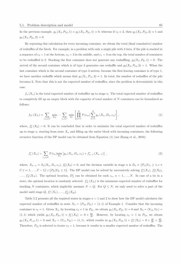
5.1. Problem description and model 85
In the previous example, g3 (X3, P12, 1) = g3 (X3, P21, 1) = 0, whereas if c3 = 2, then g3 (X3, P12, 2) = 1 and
g3 (X3, P21, 2) = 0.
By repeating this calculation for every incoming container, we obtain the total (final cumulative) number
of reshuffles of the block. For example, in a problem with only a single pile with 3 tiers, if the pile is stacked in
a sequence of c3 = 1 at the bottom, c2 = 3 in the middle, and c1 = 3 on the top, the total number of containers
to be reshuffled is 2. Stacking the first container does not generate any reshuffling, g3(X3, PE , 1) = 0. The
arrival of the second container which is of type 3 generates one reshuffle and g2(X2, P12, 3) = 1. When the
last container which is the second container of type 3 arrives, because the first-leaving container is of type 1,
we have another reshuffle which means that g1(X1, P11, 3) = 1. In total, the number of reshuffles of the pile
becomes 2. Note that this is not the expected number of reshuffles, since the problem is deterministic in this
case.
fn (Xn) is the total expected number of reshuffles up to stage n. The total expected number of reshuffles
to completely fill up an empty block with the capacity of total number of N containers can be formulated as
follows:
fN (XN ) =∑
cN∈C
minDN
· · ·∑c1∈C
minD1
[N∏
m=1
P (cm)N∑
n=1
gn (Xn, Dn, cn)
], (1)
where, f∗0 (X0) = 0. It can be concluded that in order to minimize the total expected number of reshuffles
up to stage n, starting from state Xn and filling up the entire block with incoming containers, the following
recursive function of the DP model can be obtained from Equation (1) (see Zhang et al., 2010).
f∗n (Xn) =
∑cn∈C
P (cn)minDn
[gn (Xn, Dn, cn) + f∗
n−1 (Xn−1)], (2)
where, Xn−1 = Sn(Xn, Dn, cn), f∗0 (X0) = 0, and the decision variable in stage n is Dn ∈ {Pct|Vct ≥ 1, c ∈
C, t = 1, . . . , T − 1} ∪ {PE |VE ≥ 1}. The DP model can be solved by successively solving f∗1 (X1), f
∗2 (X2),
. . . , f∗N (XN ). The optimal location, D∗
n can be obtained for each cn, n = 1, . . . , N . In case of a tie in a
state, the optimal location is randomly selected. f∗N (XN ) is the minimum expected number of reshuffles for
stacking N containers, which implicitly assumes N = Q. For Q ≤ N , we only need to solve a part of the
model until stage Q, f∗1 (X1) , . . . , f
∗Q (XQ).
Table 5.2 presents all the required states in stages n = 1 and 2 to show how the DP model calculates the
expected number of reshuffles in state X3 = (P12, P21) = (1, 1) of Example 1. Consider that the incoming
container is c3 = 1. Given X3, by locating c3 = 1 in P21, we obtain g3 (X3, P21, 1) = 0 and X2 = (V12, VF ) =
(1, 1) which yields g3 (X3, P21, 1) + f∗2 (X2) = 0 + 60
36 . However, by locating c3 = 1 in P12, we obtain
g3 (X3, P1,2, 1) = 0 and X2 = (V11, V21) = (1, 1) , which results in g3 (X3, P12, 1) + f∗2 (X2) = 0 + 49
36 < 6036 .
Therefore, P12 is selected to locate c3 = 1, because it results in a smaller expected number of reshuffles. The
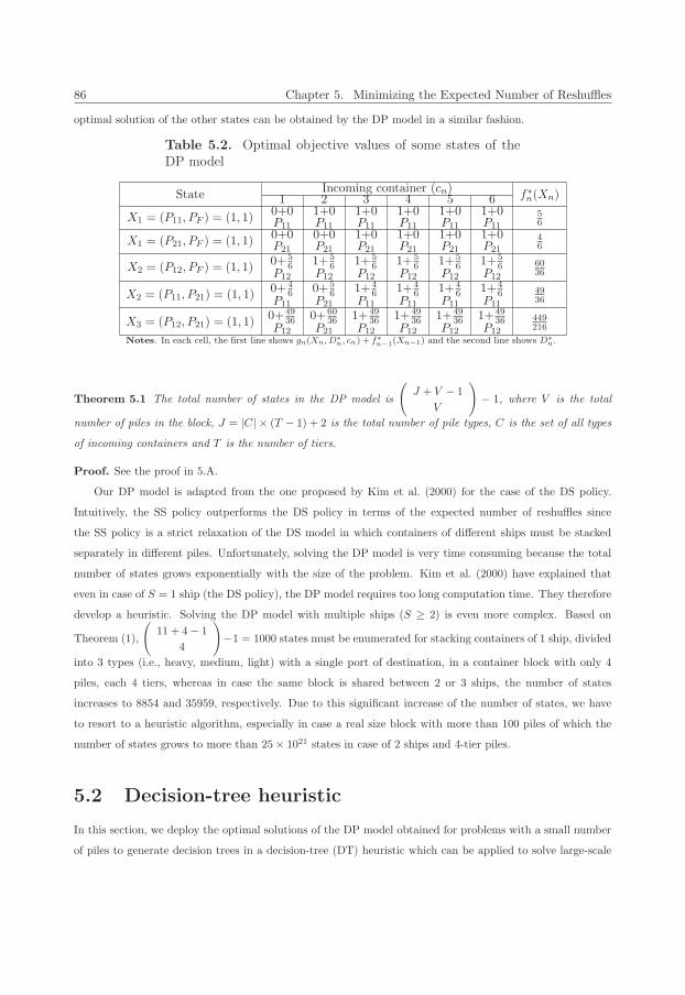
86 Chapter 5. Minimizing the Expected Number of Reshuffles
optimal solution of the other states can be obtained by the DP model in a similar fashion.
Table 5.2. Optimal objective values of some states of theDP model
StateIncoming container (cn) f∗
n(Xn)1 2 3 4 5 6
X1 = (P11, PF ) = (1, 1)0+0 1+0 1+0 1+0 1+0 1+0 5
6P11 P11 P11 P11 P11 P11
X1 = (P21, PF ) = (1, 1)0+0 0+0 1+0 1+0 1+0 1+0 4
6P21 P21 P21 P21 P21 P21
X2 = (P12, PF ) = (1, 1)0+5
6 1+56 1+5
6 1+56 1+5
6 1+56 60
36P12 P12 P12 P12 P12 P12
X2 = (P11, P21) = (1, 1)0+4
6 0+56 1+4
6 1+46 1+4
6 1+46 49
36P11 P21 P11 P11 P11 P11
X3 = (P12, P21) = (1, 1)0+49
36 0+6036 1+49
36 1+4936 1+49
36 1+4936 449
216P12 P21 P12 P12 P12 P12Notes. In each cell, the first line shows gn(Xn, D∗
n, cn) + f∗n−1(Xn−1) and the second line shows D∗
n.
Theorem 5.1 The total number of states in the DP model is
(J + V − 1
V
)− 1, where V is the total
number of piles in the block, J = |C| × (T − 1) + 2 is the total number of pile types, C is the set of all types
of incoming containers and T is the number of tiers.
Proof. See the proof in 5.A.
Our DP model is adapted from the one proposed by Kim et al. (2000) for the case of the DS policy.
Intuitively, the SS policy outperforms the DS policy in terms of the expected number of reshuffles since
the SS policy is a strict relaxation of the DS model in which containers of different ships must be stacked
separately in different piles. Unfortunately, solving the DP model is very time consuming because the total
number of states grows exponentially with the size of the problem. Kim et al. (2000) have explained that
even in case of S = 1 ship (the DS policy), the DP model requires too long computation time. They therefore
develop a heuristic. Solving the DP model with multiple ships (S ≥ 2) is even more complex. Based on
Theorem (1),
(11 + 4− 1
4
)−1 = 1000 states must be enumerated for stacking containers of 1 ship, divided
into 3 types (i.e., heavy, medium, light) with a single port of destination, in a container block with only 4
piles, each 4 tiers, whereas in case the same block is shared between 2 or 3 ships, the number of states
increases to 8854 and 35959, respectively. Due to this significant increase of the number of states, we have
to resort to a heuristic algorithm, especially in case a real size block with more than 100 piles of which the
number of states grows to more than 25× 1021 states in case of 2 ships and 4-tier piles.
5.2 Decision-tree heuristic
In this section, we deploy the optimal solutions of the DP model obtained for problems with a small number
of piles to generate decision trees in a decision-tree (DT) heuristic which can be applied to solve large-scale
5.2. Decision-tree heuristic 87
problems with an a realistic number of piles. A tree classifies a database (i.e., the DP results) and helps to
make fast and comprehensible decisions (Quinlan, 1986). It consists of nodes where a logical decision must
be made and connecting branches that are chosen according to the result of this decision. The nodes and
branches that are followed constitute a sequential path through a decision tree that reaches a final decision
in the end.
The intuition for using the DT approach is as follows. Every state of a block can be represented by a
path, where the decision where to locate the next incoming container in that state is given by the last node
in that path. Collecting all these paths together constructs a decision tree. By increasing the size of the
problem in terms of the number of piles, the number of paths grows exponentially fast. The reason is that
we need to represent every state of the block with an individual path and according to Theorem (5.1), the
number of states in the DP model increases exponentially. So, it is difficult to find a specific path in the tree
to make a quick decision. We therefore simplify the tree by merging some of its paths. We then generalize
the merged paths so that they can represent the states of a larger scale problem. These trees however, might
lead to rather poor solutions as not all paths are represented, so we improve them with better paths, if the
optimal DP results are available. The three types of trees that result from this approach are called Basic,
Simplified and Generalized trees, and are more formally defined in the following three steps:
1. Step 1. Representing the optimal results of the DP as basic decision trees: In this phase, we represent
all states of the DP model for small-scale problems as basic decision trees. In these trees, each state and
its corresponding decision is illustrated by a path where nodes represent the pile types and weighted
links represent the number of piles per pile type in the current state. Decisions can be found in the
last node of each path. The basic decision trees are quite helpful for solving small-scale problems.
However, the number of paths of the trees grows exponentially and solving the problem becomes time
consuming as the size of the problem increases.
2. Step 2. Simplifying and generalizing the basic decision trees: This phase simplifies the basic decision
trees, generated in the previous step so that the solution can be obtained more quickly. Furthermore,
we generalize them to blocks with a larger number of piles. The simplification can be carried out by
clustering multiple paths of the decision trees with the same decision as a single path. Simplifying
the decision trees significantly decreases the number of paths. These trees can be used for quickly
solving small-scale problems which are already solved by the DP model. We need to generalize them
so that they can solve real-scale problems. Generalizing is realized by using the decisions of simplified
decision trees for problems with larger number of piles. The generalized decision trees can quickly
make decisions for large-scale problems since they have few paths, whereas the DP model needs to
evaluate an enormous number of states.
3. Step 3. Improving the generalized decision trees: If the DP results for larger size problems are available,
the generalized decision trees generated in step 2 can be improved to more precisely solve larger
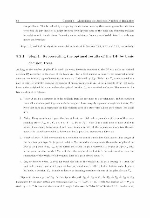
88 Chapter 5. Minimizing the Expected Number of Reshuffles
size problems. This is realized by comparing the decisions made by the current generalized decision
trees and the DP model of a larger problem for a specific state of the block and removing possible
inconsistencies in the decisions. Removing an inconsistency from a generalized decision tree adds new
nodes and branches.
Steps 1, 2, and 3 of the algorithm are explained in detail in Sections 5.2.1, 5.2.2, and 5.2.3, respectively.
5.2.1 Step 1. Representing the optimal results of the DP by basic
decision trees
As long as the number of piles V is small, for every incoming container c, the DP can make an optimal
decision D∗n according to the state of the block Xn. For a fixed number of piles V , we construct a basic
decision tree for every type of incoming container c ∈ C, denoted by BcV . Each state Xn is represented as a
path in this tree basically counting the number of piles of each type in Xn. A path consists of the root node,
inner nodes, weighted links, and defines the optimal decision D∗n in a so-called leaf node. The elements of a
tree are defined as follows:
1. Paths. A path is a sequence of nodes and links from the root node to a decision node. In basic decision
trees, all nodes in a path together with the weighted links uniquely represent a single block state, Xn.
Note that each path represents the full representation of a state with all the zero entries (see Table
5.1).
2. Nodes. Every node in each path that has at least one child node represents a pile type of the corre-
sponding state (Pnt, n ∈ C, 1 ≤ t ≤ T − 1, PF or PE). Node B is a child node of node A if it is
located immediately below node A and linked to node A. We call the topmost node of a tree the root
node. It is the reference point to follow and find a path that represents a DP state.
3. Weighted links. A link corresponds to a condition to branch a node into child nodes. The weight of
the link from pile type Pnt (a parent node) to Pml (a child node) represents the number of piles of the
type of the parent node, Vnt, in the current state that the path represents. If no pile of type Pnt exist
in the path, in other words if Vnt = 0, then the weight of the link is 0. In basic decision trees, the
summation of the weights of all weighted links in a path always equals V .
4. Leaf or decision nodes. A node for which the sum of the weights in the path leading to it from the
root node equals V and which does not have any child node is called a leaf or decision node. In every
leaf node, a decision, Dn, is made to locate an incoming container c in one of the piles of state Xn.
Figure 5.1 shows a part of B12. In this figure, the path P130→ P12
1→ P110→ P23
0→ P220→ P21
1→ P12
highlighted by the gray dotted arcs represents state X3 = (V12, V21) = (1, 1) with the decision D∗3 = P 12 to
stack c3 = 1. This is one of the states of Example 1 discussed in Table 5.1 of Section 5.1.2. Furthermore,
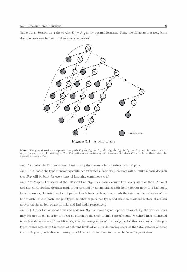
5.2. Decision-tree heuristic 89
Table 5.2 in Section 5.1.2 shows why D∗3 = P 12 is the optimal location. Using the elements of a tree, basic
decision trees can be built in 4 sub-steps as follows:
Figure 5.1. A part of B12
Note. The gray dotted arcs represent the path P130→ P12
1→ P110→ P23
0→ P220→ P21
1→ P12, which corresponds toX3 = (V12, V21) = (1, 1) with D∗
3 = P12. The paths in the contour specify the states in which V13 > 1. In all these sates, theoptimal decision is P13.
Step 1.1. Solve the DP model and obtain the optimal results for a problem with V piles.
Step 1.2. Choose the type of incoming container for which a basic decision trees will be built: a basic decision
tree BcV will be built for every type of incoming container c ∈ C.
Step 1.3. Map all the states of the DP model on BcV : in a basic decision tree, every state of the DP model
and the corresponding decision made is represented by an individual path from the root node to a leaf node.
In other words, the total number of paths of each basic decision tree equals the total number of states of the
DP model. In each path, the pile types, number of piles per type, and decision made for a state of a block
appear on the nodes, weighted links and leaf node, respectively.
Step 1.4. Order the weighted links and nodes on BcV : without a good representation of Xn, the decision trees
may become large. In order to speed up searching the trees to find a specific state, weighted links connected
to each node, are sorted from left to right in decreasing order of their weights. Furthermore, we sort the pile
types, which appear in the nodes of different levels of BcV , in decreasing order of the total number of times
that each pile type is chosen in every possible state of the block to locate the incoming container.
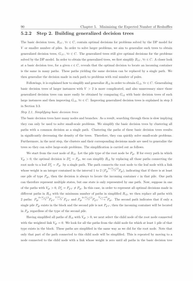
90 Chapter 5. Minimizing the Expected Number of Reshuffles
5.2.2 Step 2. Building generalized decision trees
The basic decision trees, BcV , ∀c ∈ C, contain optimal decisions for problems solved by the DP model for
V or smaller number of piles. In order to solve larger problems, we aim to generalize such trees to obtain
generalized decision trees, GcV , ∀c ∈ C. The generalized trees still give optimal decisions for the problems
solved by the DP model. In order to obtain the generalized trees, we first simplify BcV , ∀c ∈ C. A closer look
at a basic decision tree, for a given c ∈ C, reveals that the optimal decision to locate an incoming container
is the same in many paths. These paths yielding the same decision can be replaced by a single path. We
then generalize the decision made in each path to problems with real number of pules.
Followings, it is explained how to simplify and generalize Bc2 in order to obtain Gc2, ∀c ∈ C. Generalizing
basic decision trees of larger instances with V > 2 is more complicated, and also unnecessary since those
generalized decision trees can more easily be obtained by comparing Gc2 with basic decision trees of such
large instances and then improving Gc2, ∀c ∈ C. Improving generalized decision trees is explained in step 3
in Section 3.3.
Step 2.1. Simplifying basic decision trees
The basic decision trees have many nodes and branches. As a result, searching through them is slow implying
they can only be used to solve small-scale problems. We simplify the basic decision trees by clustering all
paths with a common decision as a single path. Clustering the paths of these basic decision trees results
in significantly decreasing the density of the trees. Therefore, they can quickly solve small-scale problems.
Furthermore, in the next step, the clusters and their corresponding decisions made are used to generalize the
trees so they can solve large-scale problems. The simplification is carried out as follows.
We start from the root node of Bc2. Let the pile type of the root node be Pqt. If for every path in which
Vqt > 0, the optimal decision is D∗n = Pqt, we can simplify Bc2 by replacing all those paths connecting the
root node to a leaf D∗n = Pqt by a single path. The path connects the root node to the leaf node with a link
whose weight is an integer contained in the interval 1 to 2 (Pqt0<Vqt≤2−→ Pqt), indicating that if there is at least
one pile of type Pqt, then the decision is always to locate the incoming container c in that pile. One path
can therefore represent multiple states, but one state is only represented by one path. Now, suppose in one
of the paths with Vqt > 0, D∗n = Pq′t′ �= Pqt. In this case, in order to represent all optimal decisions made in
different paths in Bc2 with the minimum number of paths in simplified Bc2, we then replace all paths with
2 paths: Pqt0<Vqt≤2−→ Pq′t′
1≤Vq′t′−→ Pq′t′ and Pqt0<Vqt≤2−→ Pq′t′
Vq′t′=0−→ Pqt. The second path indicates that if only a
single pile Pqt exists in the block and the second pile is not Pq′t′ , then the incoming container will be located
in Pqt regardless of the type of the second pile.
Having simplified all paths of Bc2 with Vqt > 0, we next select the child node of the root node connected
with the weighted link Vqt = 0. We look for all the paths from the child node for which at least 1 pile of that
type exists in the block. These paths are simplified in the same way as we did for the root node. Note that
only that part of the path connected to this child node will be simplified. This is repeated by moving to a
node connected to the child node with a link whose weight is zero until all paths in the basic decision tree
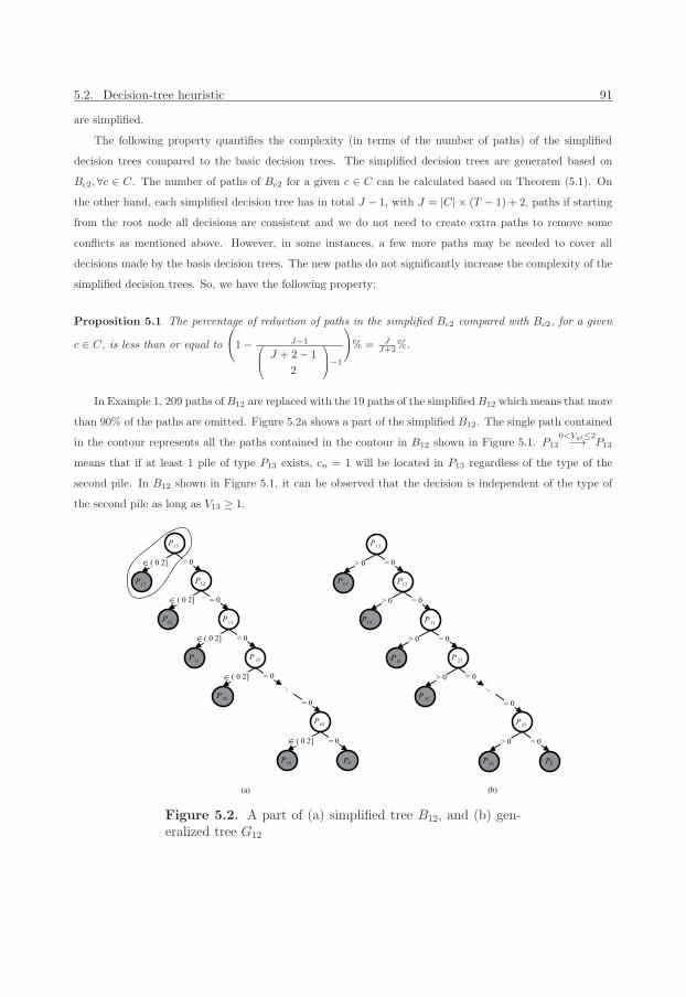
5.2. Decision-tree heuristic 91
are simplified.
The following property quantifies the complexity (in terms of the number of paths) of the simplified
decision trees compared to the basic decision trees. The simplified decision trees are generated based on
Bc2, ∀c ∈ C. The number of paths of Bc2 for a given c ∈ C can be calculated based on Theorem (5.1). On
the other hand, each simplified decision tree has in total J − 1, with J = |C| × (T − 1) + 2, paths if starting
from the root node all decisions are consistent and we do not need to create extra paths to remove some
conflicts as mentioned above. However, in some instances, a few more paths may be needed to cover all
decisions made by the basis decision trees. The new paths do not significantly increase the complexity of the
simplified decision trees. So, we have the following property:
Proposition 5.1 The percentage of reduction of paths in the simplified Bc2 compared with Bc2, for a given
c ∈ C, is less than or equal to
(1− J−1⎛
⎜⎝J + 2− 1
2
⎞⎟⎠−1
)% = J
J+2%.
In Example 1, 209 paths of B12 are replaced with the 19 paths of the simplified B12 which means that more
than 90% of the paths are omitted. Figure 5.2a shows a part of the simplified B12. The single path contained
in the contour represents all the paths contained in the contour in B12 shown in Figure 5.1. P130<Vqt≤2−→ P13
means that if at least 1 pile of type P13 exists, cn = 1 will be located in P13 regardless of the type of the
second pile. In B12 shown in Figure 5.1, it can be observed that the decision is independent of the type of
the second pile as long as V13 ≥ 1.
Figure 5.2. A part of (a) simplified tree B12, and (b) gen-eralized tree G12
92 Chapter 5. Minimizing the Expected Number of Reshuffles
Step 2.2. Generalizing simplified basic decision trees
Simplified decision trees cannot be used to solve small-scale problems. The reason is that all weighted links
are limited to at most two piles and the summation of the weights of all weighted links in a path always
equals two piles. We aim to generalize decisions made by the simplified decision trees so that we can solve
a block with a large number of piles. As a result, one obvious solution to generalize the simplified decision
trees is to remove the upper bounds. The generalized decision trees generated in this way can be used to
solve larger problems with more than two piles. These trees still give optimal decisions for the problems with
two piles.
Figure 5.2b depicts G12 of Example 1. This trees is generated by removing the upper bounds from the
weighted links of B12. In this tree, to make decision for any state of the block with any number of piles, we
start from the root node. If V13 > 0 in the block, an incoming container of type 1 will be located in P13
regardless of the number of piles in the block (V > 2). Otherwise, we check P12, if V12 > 0, the incoming
container will be located there; otherwise, we will continue further down the tree until we find a pile type of
which at least one pile exists in the block.
The following property quantifies the complexity (in terms of the number of paths) of Gc2, compared
to BcV , for a given c ∈ C and a realistic number of piles. The number of paths of BcV , ∀c ∈ C, can be
calculated based on Theorem (5.1), since each of them includes all paths from the DP model. The number
of paths in Gc2, for a give c ∈ C, is in total J − 1, if the corresponding simplified Bc2 does not have extra
branches to cover all decisions of Bc2. Extra branches however do not significantly increase the complexity.
We can formulate this as follows.
Proposition 5.2 The percentage of reduction of paths in Gc2, generated based on the simplified Bc2, com-
pared with BcV , for a given c ∈ C, is less than or equal to
(1− J−1⎛
⎜⎝J + V − 1
V
⎞⎟⎠−1
)%.
In Example 1, G12 shown in Figure 5.2b has 19 paths, whereas B13 and B14 have 1539 and 8854 paths,
respectively. As a result, G12 can make decision for problems with three and four piles where the number of
paths in G12 is 98% and 99% less than B13 and B14, respectively. Similarly, the complexity of larger basic
decision trees can be compared with G12.
5.2.3 Step 3. Improving the generalized decision trees
A generalized decision tree, Gci, ∀c ∈ C, can be improved using a basic decision tree, BcV , ∀c ∈ C, with
V > 2. In general, Gci, i > 2, is generated by comparing Gc,i−1 and Bci, and removing all inconsistencies.
An inconsistency occurs when the decisions made by a generalized decision tree and the optimal decision
made by a basic tree differ for the same state. There is no theoretic limit on the number of piles used to
improve the generalized decision trees. The improvement can consider all the piles in the block. However, the
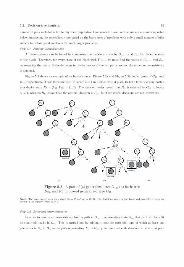
5.2. Decision-tree heuristic 93
number of piles included is limited by the computation time needed. Based on the numerical results reported
below, improving the generalized trees based on the basic trees of problems with only a small number of piles
suffices to obtain good solutions for much larger problems.
Step 3.1. Finding inconsistencies
An inconsistency can be found by comparing the decisions made by Gc,i−1 and Bci for the same state
of the block. Therefore, for every state of the block with V = i, we must find the paths in Gc,i−1 and Bci,
representing that state. If the decisions in the leaf nodes of the two paths are not the same, an inconsistency
is detected.
Figure 5.3 shows an example of an inconsistency. Figure 5.3a and Figure 5.3b depict parts of G12, and
B13, respectively. These trees are used to locate c = 1 in a block with 3 piles. In both trees the gray dotted
arcs depict state X5 = (V21, V22) = (1, 2). The decision nodes reveal that P21 is selected by G12 to locate
c5 = 1, whereas B13 shows that the optimal decision is P22. In other words, decisions are not consistent.
Figure 5.3. A part of (a) generalized tree G12, (b) basic treeB13, and (c) improved generalized tree G13
Note. The gray dotted arcs show state X5 = (V21, V22) = (1, 2). The decisions made by the basic and generalized trees areshown in the squares when c5 = 1.
Step 3.2. Removing inconsistencies
In order to remove an inconsistency from a path in Gc,i−1 representing state Xn, that path will be split
into multiple paths in Gci. This is carried out by adding a node for each pile type of which at least one
pile exists in Xn in Bci to the path representing Xn in Gc,i−1, in case that node does not exist in that path
94 Chapter 5. Minimizing the Expected Number of Reshuffles
in Gc,i−1. Each of these nodes presenting a pile type of Xn will have two links in Gci of which the weight
of one is larger than or equal to the number of piles of that type in Xn in Bci, and the other one has a
weight smaller than this number. Using only two weighted links allows us to remove the inconsistency with
a minimum increase in density of the generalized trees. Finally, to comply with the optimal decision made
by Bci, the decision in the leaf node of the path representing Xn will be the decision made by Bci and the
decision of others will be the decision made by Gc,i−1.
In order to remove the inconsistency from G12 shown in Figure 5.3a, we need to add a node for all the
pile types in X5 = (V21, V22) = (1, 2) to P130→ . . .
0→ P21>0−→ P21, which represents X5 in G12. Therefore,
P22 must be added to the path since P21 already exists in the path. In G13, the node representing P21 has
two links with the weights ≥ 1 and 0 (< 1) because V21 = 1 in X5. Furthermore, the node representing
P22 has two links with the weights ≥ 2 and < 2, as V22 = 2 in X5. Finally, the decision in the path
P130→ . . .
0→ P21≥1−→ P21
≥2−→ P22 changes to P22, since B13 has the optimal decision for X5. A part of G13
is shown in Figure 5.3c. In order to speed up the search to find a solution, we try to obtain simpler trees by
generating a smaller number of branches. Therefore, we only add and branch a node for the first and last
pile types in a state. Note that different pile types in all states are sequenced. For example, if other pile
types also exist between P21 and P22, only these two are again added and branched.
5.3 Numerical experiments
Multiple numerical experiments have been performed to evaluate the performance of the DT heuristic. In
Section 5.3.1, we compare the results of the DT heuristic with the results of the DP model. Then, through a
simulations study, we compare the SS and DS policies. In Section 5.3.2, through a case study, we show that
the DT heuristic outperforms heuristics commonly used at large container terminals in terms of the expected
number of reshuffles for real-scale problems.
The study is performed on a Notebook with 2.40 GHz Intel� CoreTM i5 processor, with 4.00 GB of
RAM and the programming language is MATLAB� 2010a.
5.3.1 Algorithm performance evaluation
In this section, we evaluate the performance of generalized decision trees by comparing them with optimal
results. We focus on a small-scale problem with seven piles and four tiers where containers of three types
should be stacked upon each other.
Table 5.3 presents the results of comparing GcV , V = 2, . . . , 7, with Bc7, c ∈ {1, 2, 3} which contains all
the states and optimal decisions for a seven pile problem. As explained in Section 5.2, Gc7 also contains all
the optimal decisions in Bc7, c ∈ {1, 2, 3} for every state. Table 5.3 shows that Gc7, c ∈ {1, 2, 3} leads to the
same decisions as Bc7, c ∈ {1, 2, 3} for stacking incoming containers in different states of the block. Using
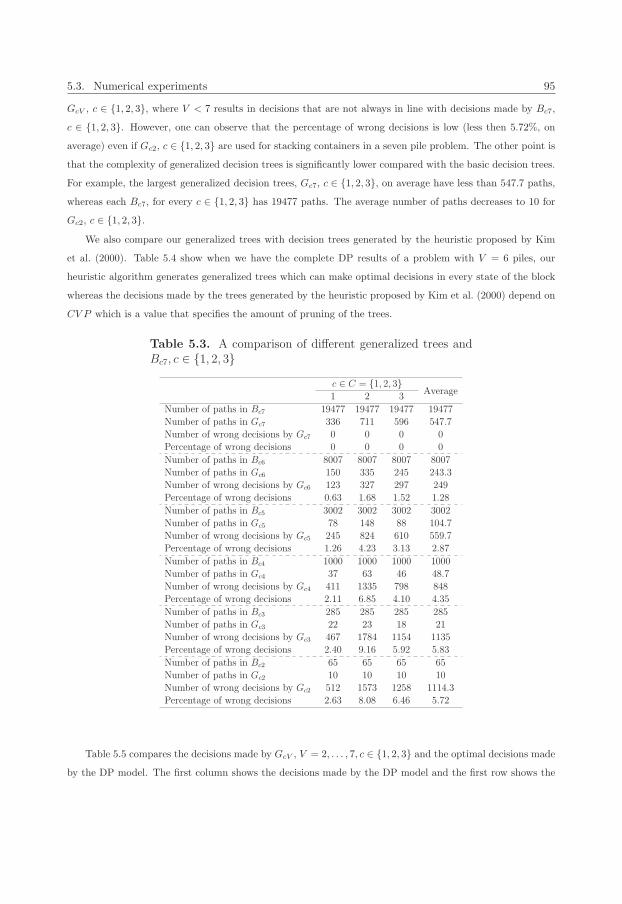
5.3. Numerical experiments 95
GcV , c ∈ {1, 2, 3}, where V < 7 results in decisions that are not always in line with decisions made by Bc7,
c ∈ {1, 2, 3}. However, one can observe that the percentage of wrong decisions is low (less then 5.72%, on
average) even if Gc2, c ∈ {1, 2, 3} are used for stacking containers in a seven pile problem. The other point is
that the complexity of generalized decision trees is significantly lower compared with the basic decision trees.
For example, the largest generalized decision trees, Gc7, c ∈ {1, 2, 3}, on average have less than 547.7 paths,
whereas each Bc7, for every c ∈ {1, 2, 3} has 19477 paths. The average number of paths decreases to 10 for
Gc2, c ∈ {1, 2, 3}.We also compare our generalized trees with decision trees generated by the heuristic proposed by Kim
et al. (2000). Table 5.4 show when we have the complete DP results of a problem with V = 6 piles, our
heuristic algorithm generates generalized trees which can make optimal decisions in every state of the block
whereas the decisions made by the trees generated by the heuristic proposed by Kim et al. (2000) depend on
CV P which is a value that specifies the amount of pruning of the trees.
Table 5.3. A comparison of different generalized trees andBc7, c ∈ {1, 2, 3}
c ∈ C = {1, 2, 3}Average
1 2 3
Number of paths in Bc7 19477 19477 19477 19477
Number of paths in Gc7 336 711 596 547.7
Number of wrong decisions by Gc7 0 0 0 0
Percentage of wrong decisions 0 0 0 0
Number of paths in Bc6 8007 8007 8007 8007
Number of paths in Gc6 150 335 245 243.3
Number of wrong decisions by Gc6 123 327 297 249
Percentage of wrong decisions 0.63 1.68 1.52 1.28
Number of paths in Bc5 3002 3002 3002 3002
Number of paths in Gc5 78 148 88 104.7
Number of wrong decisions by Gc5 245 824 610 559.7
Percentage of wrong decisions 1.26 4.23 3.13 2.87
Number of paths in Bc4 1000 1000 1000 1000
Number of paths in Gc4 37 63 46 48.7
Number of wrong decisions by Gc4 411 1335 798 848
Percentage of wrong decisions 2.11 6.85 4.10 4.35
Number of paths in Bc3 285 285 285 285
Number of paths in Gc3 22 23 18 21
Number of wrong decisions by Gc3 467 1784 1154 1135
Percentage of wrong decisions 2.40 9.16 5.92 5.83
Number of paths in Bc2 65 65 65 65
Number of paths in Gc2 10 10 10 10
Number of wrong decisions by Gc2 512 1573 1258 1114.3
Percentage of wrong decisions 2.63 8.08 6.46 5.72
Table 5.5 compares the decisions made by GcV , V = 2, . . . , 7, c ∈ {1, 2, 3} and the optimal decisions made
by the DP model. The first column shows the decisions made by the DP model and the first row shows the
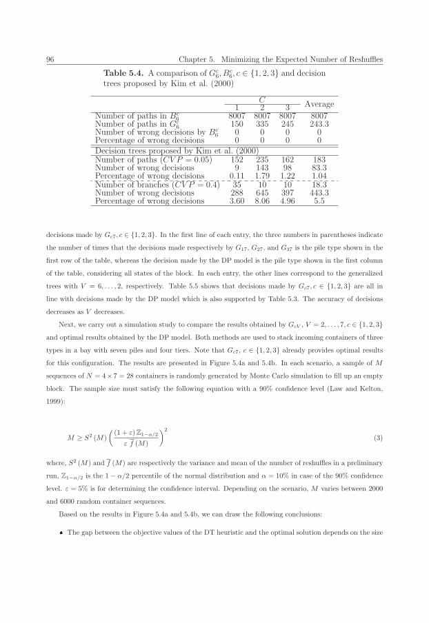
96 Chapter 5. Minimizing the Expected Number of Reshuffles
Table 5.4. A comparison of Gc6, B
c6, c ∈ {1, 2, 3} and decision
trees proposed by Kim et al. (2000)
C Average1 2 3Number of paths in Bc
6 8007 8007 8007 8007Number of paths in Gc
6 150 335 245 243.3Number of wrong decisions by Bc
6 0 0 0 0Percentage of wrong decisions 0 0 0 0Decision trees proposed by Kim et al. (2000)Number of paths (CV P = 0.05) 152 235 162 183Number of wrong decisions 9 143 98 83.3Percentage of wrong decisions 0.11 1.79 1.22 1.04Number of branches (CV P = 0.4) 35 10 10 18.3Number of wrong decisions 288 645 397 443.3Percentage of wrong decisions 3.60 8.06 4.96 5.5
decisions made by Gc7, c ∈ {1, 2, 3}. In the first line of each entry, the three numbers in parentheses indicate
the number of times that the decisions made respectively by G17, G27, and G37 is the pile type shown in the
first row of the table, whereas the decision made by the DP model is the pile type shown in the first column
of the table, considering all states of the block. In each entry, the other lines correspond to the generalized
trees with V = 6, . . . , 2, respectively. Table 5.5 shows that decisions made by Gc7, c ∈ {1, 2, 3} are all in
line with decisions made by the DP model which is also supported by Table 5.3. The accuracy of decisions
decreases as V decreases.
Next, we carry out a simulation study to compare the results obtained by GcV , V = 2, . . . , 7, c ∈ {1, 2, 3}and optimal results obtained by the DP model. Both methods are used to stack incoming containers of three
types in a bay with seven piles and four tiers. Note that Gc7, c ∈ {1, 2, 3} already provides optimal results
for this configuration. The results are presented in Figure 5.4a and 5.4b. In each scenario, a sample of M
sequences of N = 4×7 = 28 containers is randomly generated by Monte Carlo simulation to fill up an empty
block. The sample size must satisfy the following equation with a 90% confidence level (Law and Kelton,
1999):
M ≥ S2 (M)
((1 + ε)Z1−α/2
ε f (M)
)2
(3)
where, S2 (M) and f (M) are respectively the variance and mean of the number of reshuffles in a preliminary
run, Z1−α/2 is the 1− α/2 percentile of the normal distribution and α = 10% in case of the 90% confidence
level. ε = 5% is for determining the confidence interval. Depending on the scenario, M varies between 2000
and 6000 random container sequences.
Based on the results in Figure 5.4a and 5.4b, we can draw the following conclusions:
� The gap between the objective values of the DT heuristic and the optimal solution depends on the size
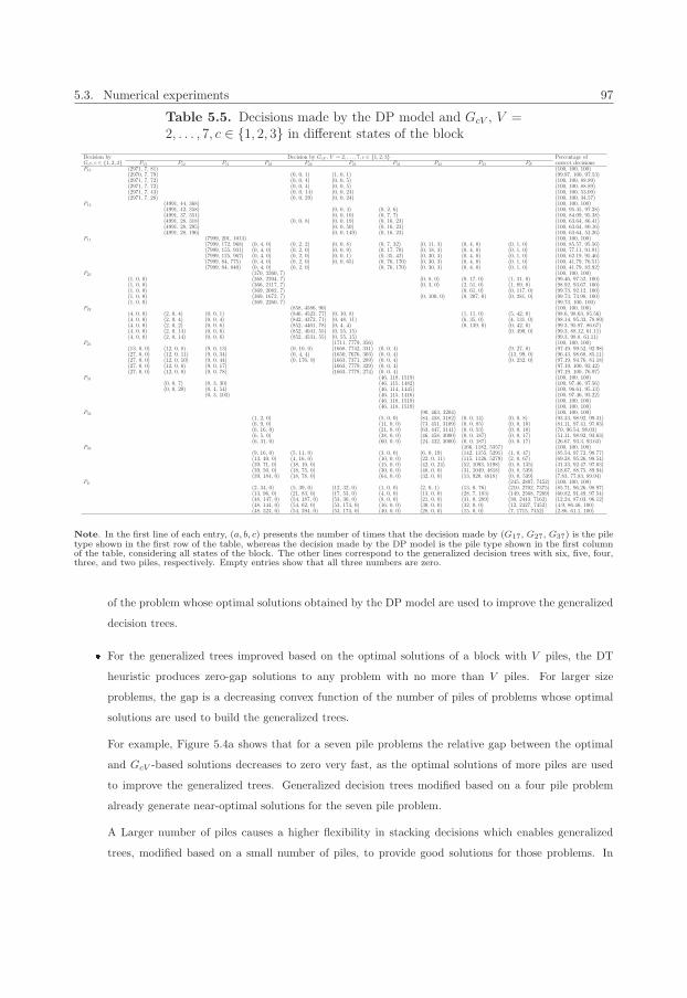
5.3. Numerical experiments 97
Table 5.5. Decisions made by the DP model and GcV , V =2, . . . , 7, c ∈ {1, 2, 3} in different states of the block
Decision by Decision by GcV , V = 2, . . . , 7, c ∈ {1, 2, 3} Percentage ofGc7, c ∈ {1, 2, 3} P13 P12 P11 P23 P22 P21 P31 P32 P33 PE correct decisionsP13 (2971, 7, 81) (100, 100, 100)
(2970, 7, 79) (0, 0, 1) (1, 0, 1) (99.97, 100, 97.53)(2971, 7, 72) (0, 0, 4) (0, 0, 5) (100, 100, 88.89)(2971, 7, 72) (0, 0, 4) (0, 0, 5) (100, 100, 88.89)(2971, 7, 43) (0, 0, 14) (0, 0, 24) (100, 100, 53.09)(2971, 7, 28) (0, 0, 29) (0, 0, 24) (100, 100, 34.57)
P12 (4991, 44, 368) (100, 100, 100)(4991, 42, 358) (0, 0, 4) (0, 2, 6) (100, 95.45, 97.28)(4991, 37, 351) (0, 0, 10) (0, 7, 7) (100, 84.09, 95.38)(4991, 28, 318) (0, 0, 8) (0, 0, 19) (0, 16, 23) (100, 63.64, 86.41)(4991, 28, 295) (0, 0, 50) (0, 16, 23) (100, 63.64, 80.16)(4991, 28, 196) (0, 0, 149) (0, 16, 23) (100, 63.64, 53.26)
P11 (7999, 201, 1013) (100, 100, 100)(7999, 172, 968) (0, 4, 0) (0, 2, 2) (0, 0, 8) (0, 7, 32) (0, 11, 3) (0, 4, 0) (0, 1, 0) (100, 85.57, 95.56)(7999, 155, 931) (0, 4, 0) (0, 2, 0) (0, 0, 9) (0, 17, 70) (0, 18, 3) (0, 4, 0) (0, 1, 0) (100, 77.11, 91.91)(7999, 125, 967) (0, 4, 0) (0, 2, 0) (0, 0, 1) (0, 35, 42) (0, 30, 3) (0, 4, 0) (0, 1, 0) (100, 62.19, 95.46)(7999, 84, 775) (0, 4, 0) (0, 2, 0) (0, 0, 65) (0, 76, 170) (0, 30, 3) (0, 4, 0) (0, 1, 0) (100, 41.79, 76.51)(7999, 84, 840) (0, 4, 0) (0, 2, 0) (0, 76, 170) (0, 30, 3) (0, 4, 0) (0, 1, 0) (100, 41.79, 82.92)
P23 (370, 2260, 7) (100, 100, 100)(1, 0, 0) (368, 2204, 7) (0, 8, 0) (0, 17, 0) (1, 31, 0) (99.46, 97.52, 100)(1, 0, 0) (366, 2117, 7) (0, 3, 0) (2, 51, 0) (1, 89, 0) (98.92, 93.67, 100)(1, 0, 0) (369, 2082, 7) (0, 61, 0) (0, 117, 0) (99.73, 92.12, 100)(1, 0, 0) (369, 1672, 7) (0, 100, 0) (0, 207, 0) (0, 281, 0) (99.73, 73.98, 100)(1, 0, 0) (369, 2260, 7) (99.73, 100, 100)
P22 (858, 4586, 90) (100, 100, 100)(4, 0, 0) (2, 0, 4) (0, 0, 1) (846, 4523, 77) (0, 10, 8) (1, 11, 0) (5, 42, 0) (98.6, 98.63, 85.56)(4, 0, 0) (2, 0, 4) (0, 0, 4) (842, 4372, 71) (0, 48, 11) (6, 35, 0) (4, 131, 0) (98.14, 95.33, 78.89)(4, 0, 0) (2, 0, 2) (0, 0, 6) (852, 4401, 78) (0, 4, 4) (0, 139, 0) (0, 42, 0) (99.3, 95.97, 86.67)(4, 0, 0) (2, 0, 14) (0, 0, 6) (852, 4041, 55) (0, 55, 15) (0, 490, 0) (99.3, 88.12, 61.11)(4, 0, 0) (2, 0, 14) (0, 0, 6) (852, 4531, 55) (0, 55, 15) (99.3, 98.8, 61.11)
P21 (1711, 7779, 356) (100, 100, 100)(13, 0, 0) (12, 0, 8) (9, 0, 13) (0, 10, 0) (1668, 7742, 331) (0, 0, 4) (9, 27, 0) (97.49, 99.52, 92.98)(27, 0, 0) (12, 0, 11) (9, 0, 34) (0, 4, 4) (1650, 7676, 303) (0, 0, 4) (13, 99, 0) (96.43, 98.68, 85.11)(27, 0, 0) (12, 0, 10) (9, 0, 44) (0, 176, 9) (1663, 7371, 289) (0, 0, 4) (0, 232, 0) (97.19, 94.76, 81.18)(27, 0, 0) (12, 0, 6) (9, 0, 17) (1663, 7779, 329) (0, 0, 4) (97.19, 100, 92.42)(27, 0, 0) (12, 0, 0) (9, 0, 78) (1663, 7779, 274) (0, 0, 4) (97.19, 100, 76.97)
P31 (46, 118, 1519) (100, 100, 100)(0, 0, 7) (0, 3, 30) (46, 115, 1482) (100, 97.46, 97.56)(0, 0, 20) (0, 4, 54) (46, 114, 1445) (100, 96.61, 95.13)
(0, 3, 103) (46, 115, 1416) (100, 97.46, 93.22)(46, 118, 1519) (100, 100, 100)(46, 118, 1519) (100, 100, 100)
P32 (90, 463, 3204) (100, 100, 100)(1, 2, 0) (5, 0, 0) (84, 458, 3182) (0, 0, 14) (0, 0, 8) (93.33, 98.92, 99.31)(6, 9, 0) (11, 0, 0) (73, 451, 3109) (0, 0, 85) (0, 0, 10) (81.11, 97.41, 97.03)(6, 16, 0) (21, 0, 0) (63, 447, 3141) (0, 0, 53) (0, 0, 10) (70, 96.54, 98.03)(6, 5, 0) (38, 0, 0) (46, 458, 3000) (0, 0, 187) (0, 0, 17) (51.11, 98.92, 93.63)(6, 31, 0) (60, 0, 0) (24, 432, 3000) (0, 0, 187) (0, 0, 17) (26.67, 93.3, 93.63)
P33 (166, 1182, 5357) (100, 100, 100)(9, 16, 0) (5, 11, 0) (3, 0, 0) (6, 0, 19) (142, 1155, 5291) (1, 0, 47) (85.54, 97.72, 98.77)(13, 40, 0) (4, 16, 0) (10, 0, 0) (22, 0, 11) (115, 1126, 5279) (2, 0, 67) (69.28, 95.26, 98.54)(39, 71, 0) (18, 10, 0) (15, 0, 0) (42, 0, 24) (52, 1093, 5198) (0, 8, 135) (31.33, 92.47, 97.03)(39, 50, 0) (18, 75, 0) (30, 0, 0) (48, 0, 0) (31, 1049, 4818) (0, 8, 539) (18.67, 88.75, 89.94)(39, 184, 0) (18, 78, 0) (64, 0, 0) (32, 0, 0) (13, 920, 4818) (0, 0, 539) (7.83, 77.83, 89.94)
PE (245, 2807, 7452) (100, 100, 100)(2, 34, 0) (5, 39, 0) (12, 32, 0) (1, 0, 0) (2, 0, 1) (13, 0, 76) (210, 2702, 7375) (85.71, 96.26, 98.97)(13, 96, 0) (21, 83, 0) (17, 53, 0) (4, 0, 0) (13, 0, 0) (28, 7, 183) (149, 2568, 7269) (60.82, 91.49, 97.54)(48, 147, 0) (54, 187, 0) (53, 30, 0) (8, 0, 0) (21, 0, 0) (31, 0, 289) (30, 2443, 7163) (12.24, 87.03, 96.12)(48, 144, 0) (54, 62, 0) (53, 174, 0) (16, 0, 0) (30, 0, 0) (32, 0, 0) (12, 2427, 7452) (4.9, 86.46, 100)(48, 524, 0) (54, 394, 0) (53, 174, 0) (40, 0, 0) (28, 0, 0) (15, 0, 0) (7, 1715, 7452) (2.86, 61.1, 100)
Note. In the first line of each entry, (a, b, c) presents the number of times that the decision made by (G17, G27, G37) is the piletype shown in the first row of the table, whereas the decision made by the DP model is the pile type shown in the first columnof the table, considering all states of the block. The other lines correspond to the generalized decision trees with six, five, four,three, and two piles, respectively. Empty entries show that all three numbers are zero.
of the problem whose optimal solutions obtained by the DP model are used to improve the generalized
decision trees.
� For the generalized trees improved based on the optimal solutions of a block with V piles, the DT
heuristic produces zero-gap solutions to any problem with no more than V piles. For larger size
problems, the gap is a decreasing convex function of the number of piles of problems whose optimal
solutions are used to build the generalized trees.
For example, Figure 5.4a shows that for a seven pile problems the relative gap between the optimal
and GcV -based solutions decreases to zero very fast, as the optimal solutions of more piles are used
to improve the generalized trees. Generalized decision trees modified based on a four pile problem
already generate near-optimal solutions for the seven pile problem.
A Larger number of piles causes a higher flexibility in stacking decisions which enables generalized
trees, modified based on a small number of piles, to provide good solutions for those problems. In
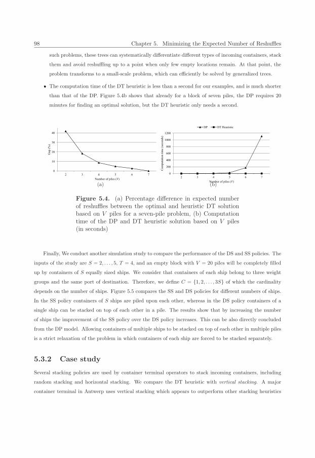
98 Chapter 5. Minimizing the Expected Number of Reshuffles
such problems, these trees can systematically differentiate different types of incoming containers, stack
them and avoid reshuffling up to a point when only few empty locations remain. At that point, the
problem transforms to a small-scale problem, which can efficiently be solved by generalized trees.
� The computation time of the DT heuristic is less than a second for our examples, and is much shorter
than that of the DP. Figure 5.4b shows that already for a block of seven piles, the DP requires 20
minutes for finding an optimal solution, but the DT heuristic only needs a second.
(a) (b)
Figure 5.4. (a) Percentage difference in expected numberof reshuffles between the optimal and heuristic DT solutionbased on V piles for a seven-pile problem, (b) Computationtime of the DP and DT heuristic solution based on V piles(in seconds)
Finally, We conduct another simulation study to compare the performance of the DS and SS policies. The
inputs of the study are S = 2, . . . , 5, T = 4, and an empty block with V = 20 piles will be completely filled
up by containers of S equally sized ships. We consider that containers of each ship belong to three weight
groups and the same port of destination. Therefore, we define C = {1, 2, . . . , 3S} of which the cardinality
depends on the number of ships. Figure 5.5 compares the SS and DS policies for different numbers of ships.
In the SS policy containers of S ships are piled upon each other, whereas in the DS policy containers of a
single ship can be stacked on top of each other in a pile. The results show that by increasing the number
of ships the improvement of the SS policy over the DS policy increases. This can be also directly concluded
from the DP model. Allowing containers of multiple ships to be stacked on top of each other in multiple piles
is a strict relaxation of the problem in which containers of each ship are forced to be stacked separately.
5.3.2 Case study
Several stacking policies are used by container terminal operators to stack incoming containers, including
random stacking and horizontal stacking. We compare the DT heuristic with vertical stacking. A major
container terminal in Antwerp uses vertical stacking which appears to outperform other stacking heuristics
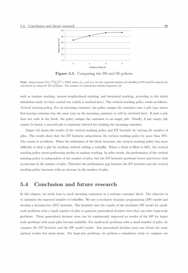
5.4. Conclusion and future research 99
Figure 5.5. Comparing the DS and SS policies
Note. Improvement (%)= fDS−fSSfDS
×100% where fDS and fSS are the expected number of reshuffles of DS and SS respectively
calculated by using the DT heuristic. The number of realizations satisfies Equation (3).
such as random stacking, nearest-neighborhood stacking, and horizontal stacking, according to the initial
simulation study we have carried out (which is omitted here). The vertical stacking policy works as follows:
Vertical stacking policy. For an incoming container, the policy assigns the container onto a pile type whose
first-leaving container has the same type as the incoming container or will be retrieved later. If such a pile
does not exist in the block, the policy assigns the container to an empty pile. Finally, if any empty pile
cannot be found, a non-full pile is randomly selected for stacking the incoming container.
Figure 5.6 shows the results of the vertical stacking policy and DT heuristic by varying the number of
piles. The results show that the DT heuristic outperforms the vertical stacking policy by more than 70%.
The reason is as follows. When the utilization of the block increases, the vertical stacking policy has more
difficulty to find a pile for stacking without adding a reshuffle. When a block is filled to 80%, the vertical
stacking policy starts performing similar to random stacking. In other words, the performance of the vertical
stacking policy is independent of the number of piles, but the DT heuristic performs better and better with
an increase in the number of piles. Therefore the performance gap between the DT heuristic and the vertical
stacking policy increases with an increase in the number of piles.
5.4 Conclusion and future research
In this chapter, we study how to stack incoming containers in a real-size container block. The objective is
to minimize the expected number of reshuffles. We use a stochastic dynamic programming (DP) model and
develop a decision-tree (DT) heuristic. The heuristic uses the results of the stochastic DP model for small-
scale problems with a small number of piles to generate generalized decision trees that can solve large-scale
problems. These generalized decision trees can be continuously improved as results of the DP for larger
scale problems with more piles become available. For small-scale problems with a small number of piles, we
compare the DT heuristic and the DP model results. Our generalized decision trees can obtain the same
optimal results but much faster. For large-size problems, we perform a simulation study to compare our
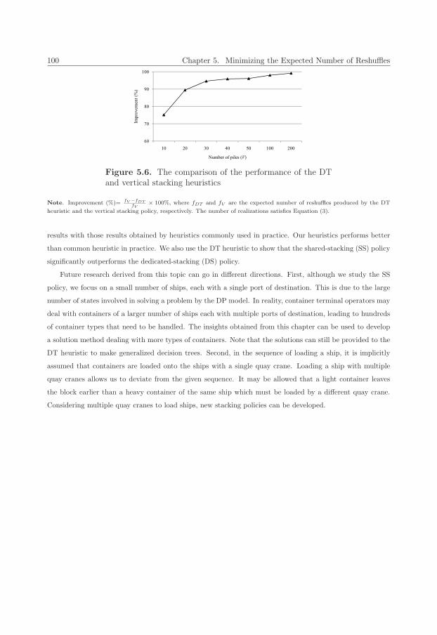
100 Chapter 5. Minimizing the Expected Number of Reshuffles
Figure 5.6. The comparison of the performance of the DTand vertical stacking heuristics
Note. Improvement (%)= fV −fDTfV
× 100%, where fDT and fV are the expected number of reshuffles produced by the DT
heuristic and the vertical stacking policy, respectively. The number of realizations satisfies Equation (3).
results with those results obtained by heuristics commonly used in practice. Our heuristics performs better
than common heuristic in practice. We also use the DT heuristic to show that the shared-stacking (SS) policy
significantly outperforms the dedicated-stacking (DS) policy.
Future research derived from this topic can go in different directions. First, although we study the SS
policy, we focus on a small number of ships, each with a single port of destination. This is due to the large
number of states involved in solving a problem by the DP model. In reality, container terminal operators may
deal with containers of a larger number of ships each with multiple ports of destination, leading to hundreds
of container types that need to be handled. The insights obtained from this chapter can be used to develop
a solution method dealing with more types of containers. Note that the solutions can still be provided to the
DT heuristic to make generalized decision trees. Second, in the sequence of loading a ship, it is implicitly
assumed that containers are loaded onto the ships with a single quay crane. Loading a ship with multiple
quay cranes allows us to deviate from the given sequence. It may be allowed that a light container leaves
the block earlier than a heavy container of the same ship which must be loaded by a different quay crane.
Considering multiple quay cranes to load ships, new stacking policies can be developed.
5.A. Proof of Theorem 5.1 101
Appendix
5.A Proof of Theorem 5.1
In our problem, we have V piles of containers and J = | {Pct|c ∈ C, t = 1, . . . , T − 1} ∪ {PE , PF } | = |C| ×(T − 1) + 2 types of piles. In each state of the block, each pile of containers has a specific type. Obviously,
multiple piles may have the same type. The number of different states of the DP model can be calculated
using the following classic combinatorial problem where a combination of size V must be chosen from J
objects and repetition is allowed (Rosen et al., 2000). The total number of combinations is
(J + V − 1
V
).
However, the total number of states of the DP model is one less. The reason is that repetition is allowed and
considering J as the total number of pile types means that in one of the states all the piles can be full which
is not feasible as no container can be located there. �

Chapter 6
Conclusions and Further Research
Container terminal operators have to make a large number of decisions every day. Among these, decisions
made regarding stacking operations at the stacking area of the terminal are studied in this dissertation. All
containers arriving from the seaside and landside must remain in this area for a period of time. Without
properly controling the stacking operations in this area, it may become a bottleneck and consequently reduce
the performance of the whole container terminal. With this motivation, in this dissertation four models have
been developed in order to make (near-) optimal decisions to deal with stacking operations.
6.1 Conclusions
In Chapter 2, we studied an automated stacking crane (ASC), stacking and retrieving containers from a
single block of containers. The block has multiple input/output (I/O) points at both seaside and landside.
The ASC moves storage containers from I/O points to the block, whereas it moves the retrieval containers
from the block to the I/O points. We formulate the problem as an asymmetrical traveling salesman problem
(ATSP) and propose a two-phase solution method to optimally solve it. In the first phase of the solution,
we develop a new merging algorithm to patch subtours of an optimal solution of the assignment problem
(AP) relaxation of the problem without adding extra travel time. In this phase, we first search for two arcs
from every two different subtours visiting a common I/O point, and swap the destinations of them to merge
the subtours. Next, based on the fact that in some arcs the ASC has multiple I/O point options with the
same travel time to visit, we can create further opportunities to merge more subtours. We show that the
first phase runs in a polynomial time, and often finds an optimal solution. Otherwise, a branch-and-bound
(B&B) algorithm is used in the second phase to find an optimal solution of the problem. In this phase, the
merging algorithm is again used in each node of the B&B tree to save computation time. The takeaways of
Chapter 2 are as follows:
� Not only the number of requests but also the number of I/O points affects the complexity of the
103
104 Chapter 6. Conclusions and Further Research
problem. The problem is NP-hard in the number of requests and I/O points.
� I/O pints can be used to develop a merging algorithm which results in efficiently solving the problem.
Since all containers have to be moved by the ASC to an I/O point or from an I/O point, the merging
algorithm can successfully solve many instances of the problem, especially larger instances. Given a
limited number of I/O points, by increasing the number of requests, the number of requests connected
to each I/O point will increase. Thus, the merging algorithm has more opportunities to patch subtours.
� The numerical experiments show that problems up to 200 requests can be optimally solved in less
than a second. Furthermore, the travel time reduction between the optimal and first-come-first-served
(FCFS) sequence is around 30%, on average. The reduction is around 14%, in case the nearest neighbor
(NN) heuristic is used to find the sequence.
In Chapter 3, we extend the problem by considering sets of open locations for storing containers. In the
case of a storage request, the ASC picks up the container from an I/O point, and drops it off in an open
storage location in the block. We formulate the problem as a generalized asymmetrical traveling salesman
problem (GATSP). However, locations in the intersection of multiple sets make the problem more complex.
Extra constraints are necessary to stack at most one container in such a location. The GATSP is NP-hard,and the new constraints increase the complexity even more. We propose a three-phase solution method to
optimally solve the problem. The main idea of the algorithm is to simplify the problem to an ATSP and
use its optimal solution to obtain an optimal GATSP solution. An optimal ATSP solution can be quickly
obtained using the solution method studied in Chapter 2. In the first phase of the algorithm, we generate
a corresponding ATSP model by pre-selecting the locations resulting in the minimum pairwise travel times.
This can be realized by redefining the original travel time matrix. In the original travel time matrix, the
pairwise travel times between two locations are calculated from the first location until the other one, whereas
in the redefined travel time matrix, the pairwise travel times are calculated from or until I/O points in an
arc, if available. We show that an optimal result of the ATSP model generated in this way is identical to an
optimal solution of the GATSP in which the new extra constraints are relaxed. In other words, an optimal
ATSP solution provides a lower bound for the problem, since pre-selection may result in a solution that one
location in the intersection of multiple sets is selected to stack multiple containers. In the second phase, we
present two special cases in which an optimal ATSP solution directly provides an optimal GATSP solution.
In the first case, sets of open locations do not overlap. In the second case, locations in the intersection of
multiple sets selected to stack containers of more than one set can be replaced with alternative open locations.
Otherwise, in the third phase, we embed the optimal ATSP solution in a B&B algorithm which tries to avoid
stacking containers of more than one set in a location by assigning it to a single set in each node. The
takeaways of Chapter 3 are as follows:
� The larger the cardinality of sets of open locations is, the harder it is to solve the problem. In fact, if
the cardinality is one for every set of open locations, the GATSP simplifies to the ATSP discussed in
6.1. Conclusions 105
Chapter 2. The ATSP can be solved in less than a second.
� The other important factor for quickly solving problems is the locations in the intersections of sets.
If there is no overlap between any two pairs of sets, no matter what the sizes of the sets are, we can
simplify the problem to an ATSP. An optimal ATSP solution directly provides an optimal GATSP
solution. As a result, it is important not only to limit the number of locations in every set but also
the locations in the overlap of the sets.
� The proposed three-phase solution method is efficient for small and medium instances. For large
instances with more than 100 requests, we propose a heuristic algorithm. The heuristic method first
finds an optimal solution of the ATSP which is generated by pre-selection of locations. In case the
solution is not a feasible GATSP solution, an AP will be used to replace all locations which are selected
to store more than one storage container by other locations with the minimum increase in the ATSP
optimal value. The numerical results show the objective value gap between our heuristic algorithm
and the lower bound is less than 1%, on average. Note that an optimal ATSP solution provides a
lower bound for the GATSP.
� Compared to the NN and FCFS heuristics used in practice, travel time savings of up to 20% and 37%,
respectively can be achieved.
� The high quality of the heuristic method is due to the fact that the ASC moves over the bays and
rows simultaneously. When the ASC moves from a storage request to another request, multiple open
locations associated to the storage request result in the minimum travel time or different travel times
which are close to each other. Therefore, the ATSP model generated by pre-selecting the empty
locations provides a good lower bound for the problem. As a result, the heuristic solution obtained
by using the AP model for replacing the multi-selected locations with the nearest empty locations is
near optimal.
In Chapter 4, we extend the problem further. In the problem studied there, two ASCs carry out the
requests, which have different priorities. We model the problem as a multiple generalized asymmetrical travel-
ing salesman problem (mGATSP-PC) including the precedence constraints and some other extra constraints.
Several practical and theoretical constraints were considered: (1) the ASCs cannot pass each other and, for
safety reasons, the ASCs must be separated by a safety distance; (2) each storage container must be stacked
in a location selected from a set of available open locations; and (3) because of waiting times and of the
presence of several container transport modes, containers have different storage and retrieval priorities. Due
to the complexity of the problem, it can only be solved exactly for small size instances. We have therefore
developed an adaptive large neighborhood search (ALNS) heuristic capable of solving instances of realistic
sizes. The takeaways of Chapter 4 are as follows:
� The ALNS is a very powerful heuristic to solve combinatorial problems. Our experiments demonstrate
the impact of the new constraints and the efficiency of our heuristic. For small instances which
106 Chapter 6. Conclusions and Further Research
can be optimally solved by CPLEX (a high-performance mathematical programming solver for linear
programming, mixed integer programming, and quadratic programming), the gaps between the ALNS
and optimal solution values are on average less than 0.34%. For large instances, compared to CPLEX
truncated after four hours, the ALNS can quickly obtain up to 6.77% better results, on average. It also
yields results that are 24% better compared with alternative less sophisticated heuristics. Furthermore,
for two relaxed problems, the ALNS obtains results that are on average within 3% of the optimal
solution values.
� The precedence constraints substantially affect the objective value. There is a big gap between the
mGATSP-PC and the mGATSP where the precedence constraints are relaxed.
In Chapter 5, we study a different problem which is indirectly related to the previous ones. The problem
is how to stack incoming containers in a real-size container block shared by containers of multiple ships. The
objective is to minimize the expected number of reshuffles. We use a stochastic dynamic programming (DP)
model and develop a decision-tree (DT) heuristic. The heuristic uses the results of the stochastic DP model
for small-scale problems with a small number of piles to generate generalized decision trees that can solve
large-scale problems. These generalized decision trees can be continuously improved as results of the DP for
larger scale problems with more piles become available. The takeaways of Chapter 5 are as follows:
� For small-scale problems with a small number of piles, we show that the gap between the optimal and
DT heuristic solutions is a decreasing convex function of the number of piles of problems of which
optimal solutions are used to improve the generalized trees. For larger scale problems, these trees
also provide near-optimal solutions since a larger number of piles results in a higher flexibility to
stack containers and to avoid reshuffling. In addition, the DT heuristic is compared with the vertical
stacking policy which is one of the good heuristics commonly used in practice. We show that the DT
heuristic significantly outperforms vertical stacking.
� Furthermore, we also use the DT heuristic to show that the shared policy significantly outperforms
the dedicated policy in which containers of a single ship are stacked on top of each other. The
shared stacking policy allows to increase the utilization of the block, whereas in the dedicated policy,
containers of only one ship can be stacked in the block.
6.2 Future research
Container terminals have received an increasing attention from the academic community due to the oppor-
tunities and challenges they offer in research. In this dissertation, some of the operational problems in the
stacking area of a container terminal are studied. The results show that major improvements can be achieved,
using the exact and heuristic models developed in this dissertation. However, there is still enough room for
conducting further research. Container terminals have seen major developments over the last decades. These
6.2. Future research 107
developments impact container terminal operations and create new opportunities for research studies. Fol-
lowings, we discuss some new research directions that are interesting from both theoretical and practical
perspectives.
Role of container terminals in networks: handling millions of containers arriving at and leaving
from the deep-sea terminals introduces many challenges such as: congestion, delay, and pollution. This has
driven container terminals to transform their static supply chains into adaptive business networks to increase
their competitiveness and robustness (Vervest and Li, 2009, Heinrich and Betts, 2003). An example is a
recent project started in the Netherlands to integrate supply chain and transportation through extending
the sea terminal gate into the hinterland as the gateway to the European hinterland Veenstra et al. (2012).
These initiatives thus shift container terminals, in addition to all their container handling activities, from
being a stock point to a flow operator. The result is a better connection between the shippers and receivers
in the network. This change comes with serious and unexplored challenges, but it also provide a tremendous
opportunity to develop a sustainable competitive advantage. The seamless flow of goods from seaports
to locations far into the hinterland will be a major enabler to prevent negative external effects from the
transport, such as congestion in seaports, congestion on motorways due to too much trucking, and enhance
the competitiveness of multimodal inland nodes for warehousing and value added activities. On the other
hand, network configurations give rise to several strategic and operational problems such as the selection
of hinterland terminals to be included in the network, the number of modalities required for transporting
containers, the percentage of containers that have to be handseled by each modality, the path that each
modality has to travel, and the terminals that each modality has to visit in its path.
Sustainable container terminals: sustainability, next to efficiency, has caught the attention of aca-
demic and professional communities during the last decade. The world has become aware of the limited
resources of the earth and the necessity to preserve the environment. Therefore, many companies are look-
ing for new methods to manage their operations more sustainably considering the environmental, economic,
and social impacts of every decision. Although with a delay, container terminals have also started to move
toward more sustainable operations. Container terminal operators are currently involved in redesigning their
operations considering that while profitable, their operations should not harm the society and environment.
As a result, traditional models in the literature which consider only profitability and efficiency have to be
modified in order to include broader considerations of the terminal’s internal and external stakeholders and
environmental impacts. The result is many new operational problems in which it is tried to reduce the
internal and external energy use, make the operations eco-friendly, and design durable facilities and handling
systems.
New technologies and automation: nowadays, traditional manual container terminals are transform-
ing into modern automated terminals which are much faster and safer. For example, manual yard cranes are
replaced with single, double, or even triple automated yard cranes to stack and retrieve containers, straddle
carriers are automated and are able to lift two TEU at the same time, modern quay cranes and yard cranes
108 Chapter 6. Conclusions and Further Research
are capable of simultaneous lifting of four TEU, traditional truck appointment systems are replaced with gate
appointment system, and etc. However, in order to be efficient, the new modern technologies and method-
ologies need careful planning. New exact or heuristic models which consider all features and constraints
introduced by automation and new technologies have to be developed.
Security and safety: security and safety are among the most important and least studied topics in
container terminal operations. Many containers daily pass through a container terminal. Handling these
containers involve many sorts of security risks such as terroristic attack and smuggling. Although the proba-
bility of such incidents is low, but the cost is extremely high. As an example, Abt (2003) estimates that the
cost of the detonation of a nuclear device in a port is within �55–�220 billion. A promising solution to avoid
these risks is inspecting all containers arriving and leaving container terminals. However, the 100% screening
is costly and time consuming, and therefore other more efficient screening policies can be developed (Bakshi
et al., 2011). Other methods such as isolating some parts of the terminal which limits access only to certified
workers may also reduce the security risk. All in all, considering the cost involved in occupance of these
incidents requires the container terminal operators and scholars to consider security at container terminals
more thoroughly. Safety on the other hand requires other measures. Container terminal operators have al-
ready acquired different methods to increase the safety in their terminals. For example, terminals ask drivers
to exit their cabs and stand inside a booth before yard cranes can load their chassis. Furthermore, many
terminals feature remotely controlled cranes which minimize exposure to potential safety hazards. However,
in order to increase the safety at terminals, many other safety regulations can be still developed.
Bibliography
Abt, C. C. (2003). The economic impact of nuclear terrorist attacks on freight transport systems in
an age of seaport vulnerability . Abt Associates, Cambridge, MA.
Admiralty and Maritime Law Guide (1972). International convention for safe containers. Re-
trieved April 04, 2012, from Admiralty and Maritime Law Guide: http://www.admiraltylawguide.
com/conven/containers1972.html.
Agarwal, R., Ergun, O (2008). Ship scheduling and network design for cargo routing in liner
shipping . Transportation Science, 42(2):175–196.
Agerschou, H., Lundgren, H., Sorensen, T., Ernst, T., Korsgaard, J., Schmidt, L. R.,
Chi, W. K. (1983). Planning and Design of Ports and Marine Terminals . John Wiley and Sons,
Chichester.
Appelgren, L. H. (1969). A column generation algorithm for a ship scheduling problem. Transporta-
tion Science, 3(1):53–68.
——– (1971). Integer programming methods for a vessel scheduling problem. Transportation Science,
5(1):64–78.
Applegate, D. L., Bixby, R. E., Chvatal, V., Cook, W. J. (2007). The Traveling Salesman
Problem: A Computational Study (Princeton Series in Applied Mathematics). Princeton University
Press.
Bakshi, N., Flynn, S. E., Gans, N. (2011). Estimating the operational impact of container inspec-
tions at international ports. Management Science, 57(1):1–20.
Barrington Freight (2012). Retrieved April 04, 2012, from Barrington Freight: http://www.
shippingtoflorida.com/florida-container-sizes.php.
Bartodziej, P., Derigs, U., Malcherek, D., Vogel, U. (2009). Models and algorithms for
solving combined vehicle and crew scheduling problems with rest constraints : an application to road
feeder service planning in air cargo transportation. OR Spectrum, 31(2):405–429.
109
110 Bibliography
Bent, R., Van Hentenryck, P. (2004). A two-stage hybrid local search for the vehicle routing
problem with time windows. Transportation Science, 38(4):515–530.
Bish, E. K., Chen, F. Y., Leong, Y. T., Nelson, B. L., Ng, J. W. C., Simchi-Levi, D. (2005).
Dispatching vehicles in a mega container terminal . OR Spectrum, 27:491–506.
Bose, J. W. (2011). Handbook of Terminal Planning . Springer, New York.
Boxxes (2012). Retrieved April 04, 2012, from Barrington Freight: http://www.boxxes.nl/.
Bozer, Y. A., Carlo, H. J. (2008). Optimizing inbound and outbound door assignments in less-
than-truckload crossdocks. IIE Transactions, 40(11):1007–1018.
Brinkmann, B. (2010). Operations systems of container terminals: A compendious overview . vol-
ume 49 of Handbook of Terminal Planning , pages 25–39. Springer Berlin / Heidelberg.
Briskorn, D., Drexl, A., Hartmann, S (2006). Inventory-based dispatching of automated guided
vehicles on container terminals. OR Spectrum, 28:611–630.
Brown, Gerald G., Graves, Glenn W., Ronen, David (1987). Scheduling ocean transportation
of crude oil . Management Science, 33(3):335–346.
Bureau International des Containers et du Transport Intermodal (BIC) (2012). Presen-
tation of the bic codes. Retrieved April 04, 2012, from BIC: http://www.bic-code.org/.
Burkard, R. E., Deineko, V. G., Van Dal, R., Van der Veen, J. A. A., Woeginger,
G. J. (1998). Well-solvable special cases of the traveling salesman problem: A survey . SIAM Re-
view, 40(3):496–546.
Carpaneto, G., Dell’Amico, M., Toth, P. (1995). Exact solution of large-scale, asymmetric
traveling salesman problems. ACM Transaction on Mathematical Software, 21(4):394–409.
Carpaneto, G., Toth, P. (1980). Some new branching and bounding criteria for the asymmetric
travelling salesman problem. Management Science, 26(7):736–743.
Caserta, M., Voß, S. (2009). A corridor method-based algorithm for the pre-marshalling problem. In
Giacobini, M., Brabazon, A., Cagnoni, S., Di Caro, G. A., Ekart, A., Esparcia-Alcazar,
A., Farooq, M., Fink, A., Machado, P. (editors), Applications of Evolutionary Computing , volume
5484 of Lecture Notes in Computer Science, pages 788–797. Springer Berlin / Heidelberg.
Cheung, R. K., Li, C. L., Lin, W. (2002). Interblock crane deployment in container terminals.
Transportation Science, 36(1):79–93.
Choo, S., Klabjan, D., Simchi-Levi, D. (2010). Multiship crane sequencing with yard congestion
constraints. Transportation Science, 44(1):98–115.
Bibliography 111
Christiansen, M., Fagerholt, K., Ronen, D. (2004). Ship routing and scheduling: Status and
perspectives. Transportation Science, 38(1):1–18.
Clausen, J. (2003). Branch and bound algorithms - principles and examples. Department of Computer
Science, University of Copenhagen.
Cordeau, J. F., Laporte, G., Legato, P., Moccia, L. (2005). Models and tabu search heuristics
for the berth-allocation problem. Transportation Science, 39:526–538.
Cosmos NV (2012). http://www.cosmosworldwide.com/ .
Crainic, G. T., Kim, K. H. (2007). Chapter 8 intermodal transportation. In Barnhart, C., La-
porte, G. (editors), Transportation, volume 14 of Handbooks in Operations Research and Management
Science, pages 467–537. Elsevier.
Cullinane, K., Song, D. W., Wang, T. F. (2005). The application of mathematical program-
ming approaches to estimating container port production efficiency . Journal of Productivity Analysis,
24(1):73–92.
Cullinane, K., Wang, T. F., Song, D. W., Ji, P. (2006). The technical efficiency of container
ports: Comparing data envelopment analysis and stochastic frontier analysis. Transportation Research
Part A: Policy and Practice, 40(4):354–374.
Daganzo, C. F. (1989). The crane scheduling problem. Transportation Research Part B: Method-
ological, 23(3):159–175.
De Castillo, B., Daganzo, C. F. (1993). Handling strategies for import containers at marine
terminals . Transportation Research Part B: Methodological, 27(2):151–166.
De Koster, R., Balk, B. M., Van Nus, W. T. I. (2009). On using dea for benchmarking container
terminals . International Journal of Operations & Production Management, 29(11):1140–1155.
De Koster, R., Van der Poort, E. (1998). Routing orderpickers in a warehouse: a comparison
between optimal and heuristic solutions . IIE Transactions, 30:469–480.
Dekker, R., Voogd, P., Asperen, E. (2007). Advanced methods for container stacking . In Kim,
K. H., Gunther, H. O. (editors), Container Terminals and Cargo Systems, pages 131–154. Springer
Berlin / Heidelberg.
Dimitrijevic, V., Saric, Z. (1997). An efficient transformation of the generalized traveling salesman
problem into the traveling salesman problem on digraphs . Information Sciences, 102(1-4):105–110.
Dorndorf, U., Schneider, F. (2010). Scheduling automated triple cross-over stacking cranes in a
container yard . OR Spectrum, 32(3):617–632.
Drewry (2011). Container Forecaster . Drewery Publications, London.
112 Bibliography
Europe Container Terminals (ECT) (2012). Retrieved April 04, 2012, from ECT: http://www.
ect.nl/imagegallery/pages/Gallery.aspx .
Evers, J. J. M., Koppers, S. A. J. (1996). Automated guided vehicle traffic control at a container
terminal . Transportation Research Part A: Policy and Practice, 30(1):21–34. ISSN 0965-8564.
Fischetti, M., Gonzalez, J. J. S., Toth, P. (1997). A branch-and-cut algorithm for the symmetric
generalized traveling salesman problem. Operations Research, 45(3):378–394.
Fischetti, M., Gonzlez, J. J. S., Toth, P. (1995). The symmetric generalized traveling salesman
polytope. Networks, 26(2):113–123.
Frederickson, G. N., Hecht, M. S., Kim, C. E. (1978). Approximation algorithms for some
routing problems . SIAM Journal on Computing, 7(2):178–193.
Froyland, G., Koch, T., Megow, N., Duane, E., Wren, H. (2008). Optimizing the landside
operation of a container terminal . OR Spectrum, 30(1):53–75.
Gharehgozli, A. H., Laporte, G., Yu, Y., De Koster, R. (2012a). Scheduling two yard cranes
handling requests with precedences in a container block with multiple open locations . Technical report,
Rotterdam.
Gharehgozli, A. H., Yu, Y., De Koster, R. (2012b). Sequencing storage and retrieval requests
in a container block with multiple open locations. Technical report, Rotterdam.
Gharehgozli, A. H., Yu, Y., De Koster, R., Udding, J. T. (2012c). A decision-tree stacking
heuristic minimizing the expected number of reshuffles at a container yard . Technical report, Rotter-
dam.
——– (2012d). Sequencing storage and retrieval requests at a container terminal . Technical report,
Rotterdam.
Gilmore, P. C., Gomory, R. E. (1964). Sequencing a One State-Variable Machine: A Solvable
Case of the Traveling Salesman Problem. Operations Research, 12(5):655–679.
Goodchild, A. V., Daganzo, C. F. (2006). Double-cycling strategies for container ships and their
effect on ship loading and unloading operations . Transportation Science, 40(4):473–483.
——– (2007). Crane double cycling in container ports: Planning methods and evaluation. Transporta-
tion Research Part B: Methodological, 41(8):875–891.
Guan, Yongpei, Cheung, RaymondK. (2004). The berth allocation problem: models and solution
methods. OR Spectrum, 26:75–92.
Gunther, H. O., Kim, K. H. (2005). Container Terminals and Automated Transport Systems -
Logistics Control Issues and Quantitative Decision Support . Springer Berlin / Heidelberg.
Bibliography 113
Hansen, P., Oguz, C., Mladenovic, N. (2008). Variable neighborhood search for minimum cost
berth allocation. European Journal of Operational Research, 191(3):636–649.
Hartmann, S. (2004). A general framework for scheduling equipment and manpower at container
terminals . OR Spectrum, 26:51–74.
Heinrich, C., Betts, B. (2003). Adapt or Die Transforming Your Supply Chain into an Adaptive
Business Network . John Wiley & Sons, New Jersey.
Hendriks, M., Laumanns, M., Lefeber, E., Udding, J. T. (2010). Robust cyclic berth planning
of container vessels . OR Spectrum, 32:501–517.
Henwood, R., Tan, T. H., Singapore Logistics Association (2006). The Practitioner’s Defini-
tive Guide: Seafreight Forwarding . SNP Reference for Institute of Policy Studies, Singapore.
Hewitt, M., Nemhauser, G. L., Savelsbergh, M. W. P. (2010). Combining exact and heuristic
approaches for the capacitated fixed-charge network flow problem. INFORMS Journal on Computing,
22(2):314–325.
Imai, A., Sun, X., Nishimura, E., Papadimitriou, S. (2005). Berth allocation in a container
port: using a continuous location space approach. Transportation Research Part B: Methodological,
39(3):199–221.
International Maritme Organization (IMO) (1977). International convention for safe con-
tainers (csc). Retrieved April 04, 2012, from IMO: http://www.imo.org/About/Conventions/
ListOfConventions/Pages/International-Convention-for-Safe-Containers-(CSC).aspx.
Kang, J., Ryu, K., Kim, K. H. (2006). Deriving stacking strategies for export containers with
uncertain weight information. Journal of Intelligent Manufacturing, 17:399–410.
Kang, S., Medina, J. C., Ouyang, Y. (2008). Optimal operations of transportation fleet for un-
loading activities at container ports. Transportation Research Part B: Methodological, 42(10):970–984.
Kim, K. H. (1997). Evaluation of the number of rehandles in container yards. Computers & Industrial
Engineering, 32(4):701–711.
Kim, K. H., Bae, J. W. (2004). A look-ahead dispatching method for automated guided vehicles in
automated port container terminals. Transportation Science, 38:224–234.
Kim, K. H., Kim, K. Y. (1999a). An optimal routing algorithm for a transfer crane in port container
terminals . Transportation Science, 33(1):17–33.
——– (1999b). Routing straddle carriers for the loading operation of containers using a beam search
algorithm. Computers & Industrial Engineering, 36(1):109–136.
114 Bibliography
Kim, K. H., Moon, K. C. (2003). Berth scheduling by simulated annealing . Transportation Research
Part B: Methodological, 37(6):541–560.
Kim, K. H., Park, K. T. (2003). A note on a dynamic space-allocation method for outbound con-
tainers . European Journal of Operational Research, 148(1):92–101.
Kim, K. H., Park, Y. M., Ryu, K. R. (2000). Deriving decision rules to locate export containers in
container yards . European Journal of Operational Research, 124(1):89–101.
Kim, K. Y., Kim, K. H. (1999c). A routing algorithm for a single straddle carrier to load export
containers onto a containership. International Journal of Production Economics, 59(1-3):425–433.
Kirkpatrick, S., Gelatt, C. D., Vecchi, M. P. (1983). Optimization by simulated annealing .
Science, 220(4598):671–680.
Kozan, E. (2000). Optimising container transfers at multimodal terminals . Mathematical and Com-
puter Modelling, 31(10-12):235–43.
Kozan, E., Preston, P. (1999). Genetic algorithms to schedule container transfers at multimodal
terminals . International Transactions in Operational Research, 6(3):311–329.
Kuhn, H. W. (1955). The Hungarian method for the assignment problem. Naval Research Logistic
Quarterly, 2:83–97.
Laporte, G. (1992). The traveling salesman problem: An overview of exact and approximate algo-
rithms. European Journal of Operational Research, 59(2):231–247.
Laporte, G., Mercure, H., Nobert, Y. (1987). Generalized travelling salesman problem through
n sets of nodes: the asymmetrical case. Discrete Applied Mathematics, 18(2):185–197.
Laporte, G., Musmanno, R., Vocaturo, F. (2010). An adaptive large neighbourhood search
heuristic for the capacitated arc-routing problem with stochastic demands. Transportation Science,
44(1):125–135.
Law, A. M., Kelton, D. M. (1999). Simulation Modeling and Analysis . McGraw-Hill Higher
Education, Boston, Massachusetts, 3rd edition.
Lawler, E. L., Lenstra, J. K., Rinnooy Kan, A. H. G., Shmoys, D. B. (1985). The Traveling
Salesman Problem, a Guided Tour of Combinatorial Optimization. John Wiley & Sons, Chichester,
UK.
Lee, B. K., Kim, K. H. (2010). Optimizing the block size in container yards . Transportation Research
Part E: Logistics and Transportation Review, 46(1):120–135.
Lee, Y., Chao, S. L. (2009). A neighborhood search heuristic for pre-marshalling export containers .
European Journal of Operational Research, 196(2):468–475.
Bibliography 115
Lee, Y., Hsu, N. Y. (2007). An optimization model for the container pre-marshalling problem.
Computers & Operations Research, 34(11):3295–3313.
Lehmann, M., Grunow, M., Gunther, H. O. (2006). Deadlock handling for real-time control of
agvs at automated container terminals. OR Spectrum, 28:631–657.
Levinson, M. (2008). The Box: How the Shipping Container Made the World Smaller and the World
Economy Bigger . Princeton University Press, Princeton, NJ.
Li, C. L., Vairaktarakis, G. L. (2004). Loading and unloading operations in container terminals.
IIE Transactions, 36(4):287–297.
Li, W., Wu, Y., Petering, M. E. H., Goh, M., de Souza, R. (2009). Discrete time model and
algorithms for container yard crane scheduling . European Journal of Operational Research, 198(1):165–
172.
Lien, Y. N., Ma, E., Wah, B. W. S. (1993). Transformation of the generalized traveling-salesman
problem into the standard traveling-salesman problem. Information Sciences, 74(1-2):177–189.
Linn, R. J., Zhang, C. Q. (2003). A heuristic for dynamic yard crane deployment in a container
terminal . IIE Transactions, 35(2):161–174.
Liu, C. I., Jula, H., Ioannou, P. A. (2002). Design, simulation, and evaluation of automated
container terminals. IEEE Transactions on Intelligent Transportation Systems, 3(1):12–26.
Liu, C. I., Jula, H., Vukadinovic, K., Ioannou, P. (2004). Automated guided vehicle system for
two container yard layouts . Transportation Research Part C: Emerging Technologies, 12(5):349–368.
Meersmans, P. J. M. (2002). Optimization of container handling systems . Ph.D. thesis, Erasmus
Research Institute of Management (ERIM), Erasmus University Rotterdam (ERIM is the joint re-
searchinstitute of the Rotterdam School of Management, Erasmus University and the Erasmus School
of Economics (ESE) at Erasmus University Rotterdam).
Midoro, R., Musso, E., Parola, F. (2005). Maritime liner shipping and the stevedoring industry:
market structure and competition strategies . Maritime Policy & Management, 32(2):89–106.
Miller, D. L., Pekny, J. F. (1991). Exact solution of large asymmetric traveling salesman problems.
Science, 251(4995):754–761.
Modality Software solutions b.v. (2012). http://www.modality.nl/products.php?lang=en.
Monaco, M. F., Sammarra, M. (2007). The berth allocation problem: A strong formulation solved
by a lagrangean approach.. Transportation Science, 41(2):265–280.
Moorthy, R., Teo, C. P. (2006). Berth management in container terminal: the template design
problem. OR Spectrum, 28:495–518.
116 Bibliography
Murty, K. G. (2007). Yard crane pools and optimum layouts for storage yards of container terminals.
Journal of Industrial and Systems Engineering, 1:190–199.
Murty, K. G., Liu, J., Wan, Y. W., Linn, R. (2005). A decision support system for operations in
a container terminal . Decision Support Systems, 39(3):309–332.
Narasimhan, A., Palekar, U. S. (2002). Analysis and algorithms for the transtainer routing problem
in container port operations. Transportation Science, 36(1):63–78.
Newman, A. M., Yano, C. A. (2000). Scheduling direct and indirect trains and containers in an
intermodal setting . Transportation Science, 34(3):256–270.
Ng, W. C. (2005). Crane scheduling in container yards with inter-crane interference. European
Journal of Operational Research, 164(1):64–78.
Ng, W. C., Mak, K. L. (2005). Yard crane scheduling in port container terminals. Applied Mathe-
matical Modelling, 29(3):263–276.
Noon, C. E., Bean, J. C. (1991). A Lagrangian based approach for the asymmetric generalized
traveling salesman problem. Operations Research, 39(4):623–632.
Pepin, A. S., Desaulniers, G., Hertz, A., Huisman, D. (2009). A comparison of five heuristics
for the multiple depot vehicle scheduling problem. Journal of Scheduling, 12:17–30.
Petering, M. E. H. (2010). Development and simulation analysis of real-time, dual-load yard truck
control systems for seaport container transshipment terminals . OR Spectrum, 32:633–661. ISSN 0171-
6468.
——– (2011a). Decision support for yard capacity, fleet composition, truck substitutability, and scalabil-
ity issues at seaport container terminals. Transportation Research Part E: Logistics and Transportation
Review, 47(1):85–103.
——– (2011b). Decision support for yard capacity, fleet composition, truck substitutability, and scalabil-
ity issues at seaport container terminals. Transportation Research Part E: Logistics and Transportation
Review, 47(1):85–103.
Petering, M. E. H., Murty, K. G. (2009). Effect of block length and yard crane deployment sys-
tems on overall performance at a seaport container transshipment terminal . Computers & Operations
Research, 36(5):1711–1725.
Petering, M. E. H., Wu, Y., Li, W., Goh, M., de Souza, R. (2009). Development and simulation
analysis of real-time yard crane control systems for seaport container transshipment terminals . OR
Spectrum, 31:801–835. ISSN 0171-6468.
Pisinger, D., Ropke, S. (2007). A general heuristic for vehicle routing problems . Computers &
Operations Research, 34(8):2403–2435.
Bibliography 117
Port of Rotterdam Authority (editor) (2012). Port Statistics. Port of Rotterdam Authority,
Rotterdam.
Quinlan, J. R. (1986). Induction of decision trees. Machine Learning, 1:81–106. ISSN 0885-6125.
Ratliff, H. D., Rosenthal, A. S. (1983). Order-Picking in a Rectangular Warehouse: A Solvable
Case of the Traveling Salesman Problem. Operations Research, 31(3):507–521.
Ronen, D. (1983). Cargo ships routing and scheduling: Survey of models and problems. European
Journal of Operational Research, 12(2):119–126.
——– (1993). Ship scheduling: The last decade. European Journal of Operational Research, 71(3):325–
333.
Ropke, S., Pisinger, D. (2006a). An adaptive large neighborhood search heuristic for the pickup and
delivery problem with time windows. Transportation Science, 40(4):455–472.
——– (2006b). A unified heuristic for a large class of vehicle routing problems with backhauls. European
Journal of Operational Research, 171(3):750–775.
Rosen, K. H., Michaels, J. G., Gross, J. L., Grossman, J. W., Shier, D. R. (editors) (2000).
Handbook of Discrete and Combinatorial Mathematics. CRC press LLC, Boca Raton, Florida.
Roy, D., De Koster, R. (2012). Modeling and design of container terminal operations. Technical
report, Rotterdam.
Sammarra, M., Cordeau, J.-F., Laporte, G., Monaco, M. F. (2007). A tabu search heuristic
for the quay crane scheduling problem. Journal of Scheduling, 10:327–336.
Shaw, P. (1997). A new local search algorithm providing high quality solutions to vehicle routing
problems. Technical report, Glasgow.
Sherali, H. D., Al-Yakoob, S. M., Hassan, M. M. (1999). Fleet management models and algo-
rithms for an oil-tanker routing and scheduling problem. IIE Transactions, 31:395–406.
Srour, F. Jordan, Van de Velde, S. (2011). Are stacker crane problems easy? a statistical study .
Computers & Operations Research, (0):–.
Stahlbock, R., Voß, S. (2008a). Operations research at container terminals: a literature update.
OR Spectrum, 30(1):1–52.
——– (2008b). Vehicle routing problems and container terminal operations an update of research. The
Vhicle Routing Problem: Latest Advances And New Challenges, 43(3):551–589.
Steenken, D., Henning, A., Freigang, S., Voß, S. (1993). Routing of straddle carriers at a
container terminal with the special aspect of internal moves. OR Spectrum, 15:167–172.
118 Bibliography
Steenken, D., Voß, S., Stahlbock, R. (2004). Container terminal operation and operations
research - a classification and literature review . OR Spectrum, (26):3–49.
Taggart, S. (1999). The 20-ton packet . Wired Magazine, 7(10):246.
United Nations: ESCAP (2007). Regional Shipping and Port Development: Container Traffic
Forecast 2007 Update. United Nations: Economic and Social Comission for Asia and the Pacific
(ESCAP), New York.
Van den Berg, J. P., Gademann, A. J. R. M. (1999). Optimal routing in an automated stor-
age/retrieval system with dedicated storage. IIE Transactions, 31(5):407.
Veenstra, A., Zuidwijk, R., Van Asperen, E. (2012). The extended gate concept for container
terminals: Expanding the notion of dry ports. Maritime Econ Logistics, 14:1479–2931.
Vervest, P., Li, Z. (2009). The Network Experience New Value From Smart Business Networks .
Springer, Berlin, Germany.
Vis, I. F. A. (2006). A comparative analysis of storage and retrieval equipment at a container terminal .
International Journal of Production Economics, 103(2):680–693.
Vis, I. F. A., Carlo, H. J. (2010). Sequencing two cooperating automated stacking cranes in a
container terminal . Transportation Science, 44(2):169–182.
Vis, I. F. A., De Koster, R. (2003). Transshipment of containers at a container terminal: An
overview . European Journal of Operational Research, 147(1):1–16.
Vis, I. F. A., De Koster, R., Peeters, L. W. P. (2001). Determination of the number of automated
guided vehicles required at a semi-automated container terminal . Journal of Operational Research
Society, 52:409–417.
Vis, I. F. A., De Koster, R., Savelsbergh, M. W. P. (2005). Minimum vehicle fleet size under
time-window constraints at a container terminal . Transportation Science, 39(2):249–260.
Vis, I. F. A., Roodbergen, K. J. (2009). Scheduling of container storage and retrieval . Operations
Research, 57(2):456–467.
Wang, F., Lim, A. (2007). A stochastic beam search for the berth allocation problem. Decision
Support Systems, 42:2186–2196.
Wang, T. F., Cullinane, K. (2006). The efficiency of european container terminals and implications
for supply chain management . Maritime Economics and Logistics, 8(1):82–99.
Wiegmans, B. W., Ubbels, B., Rietveld, P., Nijkamp, P. (2002). Investments in container
terminals: Public private partnerships in europe. International Journal of MAritime Econmics, 4:1–20.
Bibliography 119
Wiese, J., Suhl, L., Kliewer, N. (2010). Mathematical models and solution methods for optimal
container terminal yard layouts . OR Spectrum, 32(3):427–452.
Wilhelm, M. R., Ward, T. L. (1987). Solving quadratic assignment problems by simulated annealing .
IIE Transactions, 19(1):107–119.
Zhang, C., Chen, W., Shi, L., Zheng, L. (2010). A note on deriving decision rules to locate export
containers in container yards. European Journal of Operational Research, 205(2):483–485.
Zhang, C., Wan, Y. W., Liu, J., Linn, R. J. (2002). Dynamic crane deployment in container
storage yards . Transportation Research Part B: Methodological, 36(6):537–555.
Zhao, W., Goodchild, A. V. (2010). The impact of truck arrival information on container terminal
rehandling . Transportation Research Part E: Logistics and Transportation Review, 46(3):327–343.
Zhen, L., Chew, E. P., Lee, L. H. (2011). An integrated model for berth template and yard template
planning in transshipment hubs . Transportation Science, 45(4):483–504.

About the author
Amir Hossein Gharehgozli (1983) received his BSc in Industrial Engi-
neering from Sharif University of Technology in 2005 and his MSc in In-
dustrial Engineering from University of Tehran in 2008 both in Tehran,
Iran. In September 2008, he joined Rotterdam School of Management,
Erasmus University Rotterdam. His research interests include: con-
tainer yard operations, transportation, logistics and supply chain man-
agement. His research findings has been presented in many international
conferences including INFORMS Annual Meetings (2009, 2011), and Eu-
ropean Conference on Operational Research (2009). He is currently a
Postdoctoral fellow at Rotterdam School of Management, Erasmus Uni-
versity Rotterdam. He was a visiting scholar from June 2011 until September 2011 in the Department of
Information Management and Decision Science, University of Science and Technology of China, Hefei, Anhui,
China. Furthermore, he was a visiting scholar from September 2011 until December 2011 at Center Interuni-
versitaire de Recherche sur les Reseaux d’Entreprise, la Logistique et le Transport (CIRRELT), Montreal,
Quebec, Canada, where he was working with Prof. Gilbert Laporte.
121

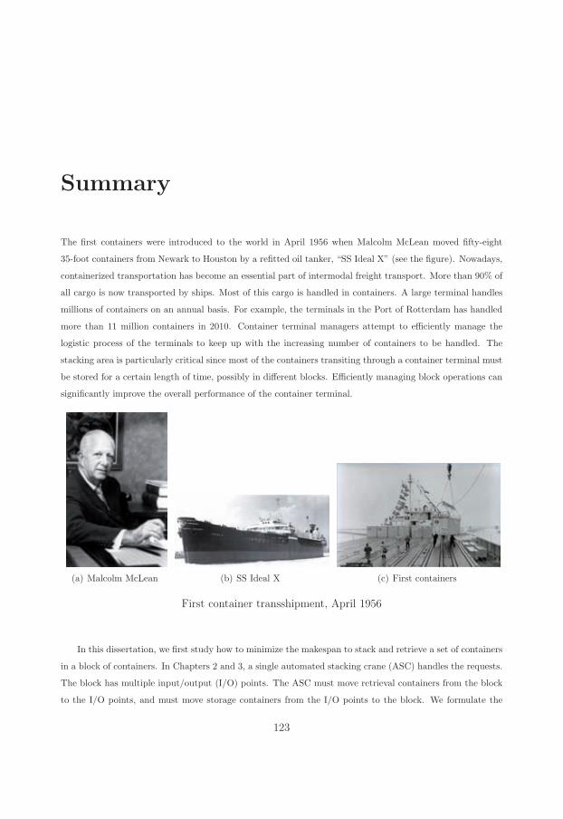
Summary
The first containers were introduced to the world in April 1956 when Malcolm McLean moved fifty-eight
35-foot containers from Newark to Houston by a refitted oil tanker, “SS Ideal X” (see the figure). Nowadays,
containerized transportation has become an essential part of intermodal freight transport. More than 90% of
all cargo is now transported by ships. Most of this cargo is handled in containers. A large terminal handles
millions of containers on an annual basis. For example, the terminals in the Port of Rotterdam has handled
more than 11 million containers in 2010. Container terminal managers attempt to efficiently manage the
logistic process of the terminals to keep up with the increasing number of containers to be handled. The
stacking area is particularly critical since most of the containers transiting through a container terminal must
be stored for a certain length of time, possibly in different blocks. Efficiently managing block operations can
significantly improve the overall performance of the container terminal.
(a) Malcolm McLean (b) SS Ideal X (c) First containers
First container transshipment, April 1956
In this dissertation, we first study how to minimize the makespan to stack and retrieve a set of containers
in a block of containers. In Chapters 2 and 3, a single automated stacking crane (ASC) handles the requests.
The block has multiple input/output (I/O) points. The ASC must move retrieval containers from the block
to the I/O points, and must move storage containers from the I/O points to the block. We formulate the
123
124 Summary
problems as continuous time integer programming models and propose exact and heuristic solution methods
to solve them. The numerical experiments reveal that the optimal makespan results are significantly shorter
than results obtained by heuristics commonly used in practice such as first-come-first-served and selecting
the nearest request. In Chapter 4, two ASCs carry out the requests. The ASCs can never pass each other and
must operate sufficiently far from each other. We formulate this problem as an integer programming model
and propose a metaheuristic algorithm to solve it. The results show that the proposed algorithm significantly
outperforms other heuristics and truncated CPLEX.
In Chapters 2–4, we consider that locations as well as destination sides of retrieval containers and I/O
points of storage containers are known. Note that in Chapter 2, each storage location has a given storage
location in the block. In contrast, in Chapters 3 and 4, each storage container can be stacked in a location
selected from a set of open locations suitable for stacking that container. Storage locations can be determined
using the methodology discussed in Chapter 5, where we use a stochastic dynamic programming model to
decide where to stack each incoming container in a block. The objective is to minimize the expected number
of reshuffles. The number of states of the dynamic programming model is overwhelming. We propose a
decision-tree heuristic algorithm to solve real instances. The heuristic uses the results of the exact model
for small-scale problems to generate generalized decision trees. These trees can be used to solve problems
with a realistic number of piles. For small-scale problems, the trees can quickly make optimal decisions. For
large-scale problems, the decision-tree heuristic significantly outperforms stacking policies commonly used
in practice. Those policies perform well as long as the utilization of the block is low. However, since they
are myopic, as the utilization increases, they start performing similar to random stacking which results in
reshuffles. Using the decision trees, we can compare the performance of a shared-stacking policy, which
allows containers of multiple ships to be stacked on top of each other, with a dedicated-stacking policy.
Shared-stacking appears to outperform dedicated-stacking.
Finally, in chapter 6, we conclude the dissertation and summarize the contributions and findings. To-
gether, the exact and heuristic methods developed in this dissertation can be used by container terminal
operators to increase the performance at the stacking area, which consequently affects the whole terminal
performance.
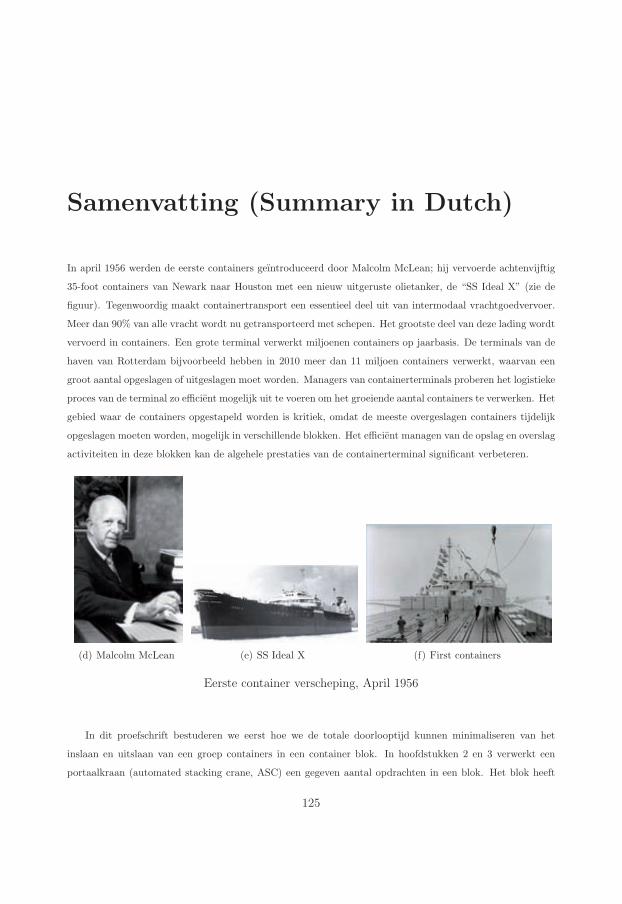
Samenvatting (Summary in Dutch)
In april 1956 werden de eerste containers geıntroduceerd door Malcolm McLean; hij vervoerde achtenvijftig
35-foot containers van Newark naar Houston met een nieuw uitgeruste olietanker, de “SS Ideal X” (zie de
figuur). Tegenwoordig maakt containertransport een essentieel deel uit van intermodaal vrachtgoedvervoer.
Meer dan 90% van alle vracht wordt nu getransporteerd met schepen. Het grootste deel van deze lading wordt
vervoerd in containers. Een grote terminal verwerkt miljoenen containers op jaarbasis. De terminals van de
haven van Rotterdam bijvoorbeeld hebben in 2010 meer dan 11 miljoen containers verwerkt, waarvan een
groot aantal opgeslagen of uitgeslagen moet worden. Managers van containerterminals proberen het logistieke
proces van de terminal zo efficient mogelijk uit te voeren om het groeiende aantal containers te verwerken. Het
gebied waar de containers opgestapeld worden is kritiek, omdat de meeste overgeslagen containers tijdelijk
opgeslagen moeten worden, mogelijk in verschillende blokken. Het efficient managen van de opslag en overslag
activiteiten in deze blokken kan de algehele prestaties van de containerterminal significant verbeteren.
(d) Malcolm McLean (e) SS Ideal X (f) First containers
Eerste container verscheping, April 1956
In dit proefschrift bestuderen we eerst hoe we de totale doorlooptijd kunnen minimaliseren van het
inslaan en uitslaan van een groep containers in een container blok. In hoofdstukken 2 en 3 verwerkt een
portaalkraan (automated stacking crane, ASC) een gegeven aantal opdrachten in een blok. Het blok heeft
125
126 Samenvatting (Summary in Dutch)
meerdere in- en output (I/O) punten. De ASC moet de uitslag containers verplaatsen van het blok naar
een I/O punt, en moet opslagcontainers verplaatsen van een I/O punt naar locaties binnen het blok. We
formuleren de problemen als continue tijd integer programmeringsmodellen en doen een voorstel voor exacte
en heuristische oplossingsmethoden om ze op te lossen. De numerieke experimenten tonen dat de optimale
doorlooptijd significant korter is dan de resultaten verkregen met in de praktijk gebruikelijke heuristieken zoals
“first-come-first-served” en het selecteren can de “nearest neighbor” container. In hoofdstuk 4 wordt het blok
bediend door twee ASC’s. De ASC’s kunnen elkaar niet passeren en moeten met voldoende afstand van elkaar
opereren. We formuleren dit probleem als een integer programmeringsmodel en stellen een meta-heuristisch
algoritme voor om dit op te lossen. Het resultaat laat zien dat het voorgestelde algoritme significant beter is
dan de andere heuristieken en CPLEX dat afgekapt wordt na een bepaalde rekentijd.
In hoofdstuk 2–4 beschouwen we locaties en bestemmingen van uitslag containers en I/O punten van
opslagcontainers als bekend. In hoofdstuk 2 had iedere opslagcontainer een gegeven opslag locatie in het
blok. In hoofdstuk 3 en 4 kan elke opslagcontainer gestapeld worden op een locatie geselecteerd uit een
aantal open locaties passend voor het opstapelen van die container. Opslaglocaties kunnen bepaald worden
met de methodologie besproken in hoofdstuk 5, waar we een stochastische dynamische programmeringsmodel
gebruiken om te bepalen waar elke inkomende container in een blok opgestapeld dient te worden. Het doel is
het minimaliseren van het verwachte aantal interne verplaatsingen (verkassingen). Het aantal toestanden van
het dynamische programmeringsmodel is overweldigend. Als oplossing introduceren we een beslissingsboom
met heuristisch algoritme om realistische cases op te lossen. De heuristiek gebruikt de resultaten van het
exacte model voor kleinschalige problemen om “generalized” beslissingsbomen te genereren. Deze bomen
kunnen gebruikt worden om problemen op te lossen met een realistisch aantal containerstapels. Voor klein-
schalige problemen kunnen deze bomen snel optimale beslissingen nemen. Voor grootschalige problemen is de
beslisboom-heuristiek significant beter dan de huidige stapelmethoden. De huidige methoden presteren goed
zolang de benutting van het blok laag is. Echter, door hun myopische werking gaan ze, zodra de blok benutting
toeneemt, steeds meer lijken op een willekeurige stapeling, wat resulteert in extra verkassingen. Gebruik mak-
end van beslisbomen, kunnen we de resultaten vergelijken van een “shared-stacking policy”, welke toestaat
dat containers van meerdere schepen op elkaar containerstapels kunnen vormen, en een “dedicated-stacking
policy”. Shared stapeling blijkt minder verkassingen te geven dan dedicated stapeling.
Tenslotte worden in hoofdstuk 6 conclusies getrokken met betrekking tot de bevindingen en bijdragen van
dit proefschrift. De exacte en heuristische methoden ontwikkeld in dit proefschrift kunnen gebruikt worden
door container terminal operators om de prestaties te verhogen in de container blok, waarmee de prestaties
van de hele terminal bınvloed kunnen worden.
ERIM Ph.D. Series Research in
Management
ERASMUS RESEARCH INSTITUTE OF MANAGEMENT
The ERIM PhD Series contains PhD dissertations in the field of Research in Management defended at Erasmus
University Rotterdam and supervised by senior researchers affiliated to the Erasmus Research Institute of
Management (ERIM). All dissertations in the ERIM PhD Series are available in full text through the ERIM
Electronic Series Portal: http://hdl.handle.net/1765/1. ERIM is the joint research institute of the Rotterdam
School of Management (RSM) and the Erasmus School of Economics at the Erasmus University Rotterdam
(EUR).
Acciaro, M., Bundling Strategies in Global Supply Chains, Promoter(s): Prof.dr. H.E. Haralambides,
EPS-2010-197-LIS, http://hdl.handle.net/1765/19742
Agatz, N.A.H., Demand Management in E-Fulfillment, Promoter(s): Prof.dr.ir. J.A.E.E. van Nunen,
EPS-2009-163-LIS, http://hdl.handle.net/1765/15425
Alexiev, A., Exploratory Innovation: The Role of Organizational and Top Management Team Social
Capital, Promoter(s): Prof.dr. F.A.J. van den Bosch & Prof.dr. H.W. Volberda, EPS-2010-208-STR,
http://hdl.handle.net/1765/20632
Asperen, E. van, Essays on Port, Container, and Bulk Chemical Logistics Optimization, Promoter(s):
Prof.dr.ir. R. Dekker, EPS-2009-181-LIS, http://hdl.handle.net/1765/17626
Assem, M.J. van den, Deal or No Deal? Decision Making under Risk in a Large-Stake TV
Game Show and Related Experiments, Promoter(s): Prof.dr. J. Spronk, EPS-2008-138-F&A,
http://hdl.handle.net/1765/13566
127
128 ERIM Ph.D. Series Research in Management
Benning, T.M., A Consumer Perspective on Flexibility in Health Care: Priority Access Pric-
ing and Customized Care, Promoter(s): Prof.dr.ir. B.G.C. Dellaert, EPS-2011-241-MKT,
http://hdl.handle.net/1765/23670
Betancourt, N.E., Typical Atypicality: Formal and Informal Institutional Conformity, Deviance, and Dy-
namics, Promoter(s): Prof.dr. B. Krug, EPS-2012-262-ORG, http://hdl.handle.net/1765/32345
Bezemer, P.J., Diffusion of Corporate Governance Beliefs: Board Independence and the Emergence of a
Shareholder Value Orientation in the Netherlands, Promoter(s): Prof.dr.ing. F.A.J. van den Bosch &
Prof.dr. H.W. Volberda, EPS-2009-192-STR, http://hdl.handle.net/1765/18458
Binken, J.L.G., System Markets: Indirect Network Effects in Action, or Inaction, Promoter(s): Prof.dr. S.
Stremersch, EPS-2010-213-MKT, http://hdl.handle.net/1765/21186
Blitz, D.C., Benchmarking Benchmarks, Promoter(s): Prof.dr. A.G.Z. Kemna & Prof.dr. W.F.C. Ver-
schoor, EPS-2011-225-F&A, http://hdl.handle.net/1765/22624
Boer-Sorban, K., Agent-Based Simulation of Financial Markets: A modular, Continuous-Time Approach,
Promoter(s): Prof.dr. A. de Bruin, EPS-2008-119-LIS, http://hdl.handle.net/1765/10870
Boon, C.T., HRM and Fit: Survival of the Fittest!?, Promoter(s): Prof.dr. J. Paauwe & Prof.dr. D.N. den
Hartog, EPS-2008-129-ORG, http://hdl.handle.net/1765/12606
Borst, W.A.M., Understanding Crowdsourcing: Effects of Motivation and Rewards on Participation and
Performance in Voluntary Online Activities, Promoter(s): Prof.dr.ir. J.C.M. van den Ende & Prof.dr.ir.
H.W.G.M. van Heck, EPS-2010-221-LIS, http://hdl.handle.net/1765/ 21914
Braun, E., City Marketing: Towards an Integrated Approach, Promoter(s): Prof.dr. L. van den Berg,
EPS-2008-142-MKT, http://hdl.handle.net/1765/13694
Brumme, W.-H., Manufacturing Capability Switching in the High-Tech Electronics Technology Life Cycle,
Promoter(s): Prof.dr.ir. J.A.E.E. van Nunen & Prof.dr.ir. L.N. Van Wassenhove, EPS-2008-126-LIS,
http://hdl.handle.net/1765/12103
Budiono, D.P., The Analysis of Mutual Fund Performance: Evidence from U.S. Equity Mutual Funds,
Promoter(s): Prof.dr. M.J.C.M. Verbeek, EPS-2010-185-F&A, http://hdl.handle.net/1765/18126
Burger, M.J., Structure and Cooptition in Urban Networks, Promoter(s): Prof.dr. G.A. van der Knaap &
Prof.dr. H.R. Commandeur, EPS-2011-243-ORG, http://hdl.handle.net/1765/26178
Burgers, J.H., Managing Corporate Venturing: Multilevel Studies on Project Autonomy, Integration,
Knowledge Relatedness, and Phases in the New Business Development Process, Promoter(s): Prof.dr.ir.
F.A.J. Van den Bosch & Prof.dr. H.W. Volberda, EPS-2008-136-STR, http://hdl.handle.net/1765/13484
ERIM Ph.D. Series Research in Management 129
Camacho, N.M., Health and Marketing; Essays on Physician and Patient Decision-making, Promoter(s):
Prof.dr. S. Stremersch, EPS-2011-237-MKT, http://hdl.handle.net/1765/23604
Carvalho de Mesquita Ferreira, L., Attention Mosaics: Studies of Organizational Attention, Pro-
moter(s): Prof.dr. P.M.A.R. Heugens & Prof.dr. J. van Oosterhout, EPS-2010-205-ORG,
http://hdl.handle.net/1765/19882
Chen, C.-M., Evaluation and Design of Supply Chain Operations Using DEA, Promoter(s): Prof.dr.
J.A.E.E. van Nunen, EPS-2009-172-LIS, http://hdl.handle.net/1765/16181
Chen, H., Individual Mobile Communication Services and Tariffs, Promoter(s): Prof.dr. L.F.J.M. Pau,
EPS-2008-123-LIS, http://hdl.handle.net/1765/11141
Defilippi Angeldonis, E.F., Access Regulation for Naturally Monopolistic Port Terminals: Lessons
from Regulated Network Industries, Promoter(s): Prof.dr. H.E. Haralambides, EPS-2010-204-LIS,
http://hdl.handle.net/1765/19881
Deichmann, D., Idea Management: Perspectives from Leadership, Learning, and Network Theory, Pro-
moter(s): Prof.dr.ir. J.C.M. van den Ende, EPS-2012-255-ORG, http://hdl.handle.net/1765/ 31174
Derwall, J.M.M., The Economic Virtues of SRI and CSR, Promoter(s): Prof.dr. C.G. Koedijk, EPS-2007-
101-F&A, http://hdl.handle.net/1765/8986
Desmet, P.T.M., In Money we Trust? Trust Repair and the Psychology of Financial Compen-
sations, Promoter(s): Prof.dr. D. De Cremer & Prof.dr. E. van Dijk, EPS-2011-232-ORG,
http://hdl.handle.net/1765/23268
Diepen, M. van, Dynamics and Competition in Charitable Giving, Promoter(s): Prof.dr. Ph.H.B.F.
Franses, EPS-2009-159-MKT, http://hdl.handle.net/1765/14526
Dietvorst, R.C., Neural Mechanisms Underlying Social Intelligence and Their Relationship with the
Performance of Sales Managers, Promoter(s): Prof.dr. W.J.M.I. Verbeke, EPS-2010-215-MKT,
http://hdl.handle.net/1765/21188
Dietz, H.M.S., Managing (Sales)People towards Perfomance: HR Strategy, Leadership & Teamwork, Pro-
moter(s): Prof.dr. G.W.J. Hendrikse, EPS-2009-168-ORG, http://hdl.handle.net/1765/16081
Doorn, S. van, Managing Entrepreneurial Orientation, Promoter(s): Prof.dr. J.J.P. Jansen, Prof.dr.ing.
F.A.J. van den Bosch & Prof.dr. H.W. Volberda, EPS-2012-258-STR, http://hdl.handle.net/1765/32166
Douwens-Zonneveld, M.G., Animal Spirits and Extreme Confidence: No Guts, No Glory, Promoter(s):
Prof.dr. W.F.C. Verschoor, EPS-2012-257-F&A, http://hdl.handle.net/1765/31914
Duca, E., The Impact of Investor Demand on Security Offerings, Promoter(s): Prof.dr. A. de Jong,
EPS-2011-240-F&A, http://hdl.handle.net/1765/26041
130 ERIM Ph.D. Series Research in Management
Eck, N.J. van, Methodological Advances in Bibliometric Mapping of Science, Promoter(s): Prof.dr.ir. R.
Dekker, EPS-2011-247-LIS, http://hdl.handle.net/1765/26509
Eijk, A.R. van der, Behind Networks: Knowledge Transfer, Favor Exchange and Performance,
Promoter(s): Prof.dr. S.L. van de Velde & Prof.dr.drs. W.A. Dolfsma, EPS-2009-161-LIS,
http://hdl.handle.net/1765/14613
Elstak, M.N., Flipping the Identity Coin: The Comparative Effect of Perceived, Projected and Desired Or-
ganizational Identity on Organizational Identification and Desired Behavior, Promoter(s): Prof.dr. C.B.M.
van Riel, EPS-2008-117-ORG, http://hdl.handle.net/1765/10723
Erken, H.P.G., Productivity, R&D and Entrepreneurship, Promoter(s): Prof.dr. A.R. Thurik, EPS-2008-
147-ORG, http://hdl.handle.net/1765/14004
Essen, M. van, An Institution-Based View of Ownership, Promoter(s): Prof.dr. J. van Oosterhout &
Prof.dr. G.M.H. Mertens, EPS-2011-226-ORG, http://hdl.handle.net/1765/22643
Feng, L., Motivation, Coordination and Cognition in Cooperatives, Promoter(s): Prof.dr. G.W.J. Hen-
drikse, EPS-2010-220-ORG, http://hdl.handle.net/1765/21680
Gertsen, H.F.M., Riding a Tiger without Being Eaten: How Companies and Analysts Tame Financial
Restatements and Influence Corporate Reputation, Promoter(s): Prof.dr. C.B.M. van Riel, EPS-2009-171-
ORG, http://hdl.handle.net/1765/16098
Gijsbers, G.W., Agricultural Innovation in Asia: Drivers, Paradigms and Performance, Promoter(s):
Prof.dr. R.J.M. van Tulder, EPS-2009-156-ORG, http://hdl.handle.net/1765/14524
Ginkel-Bieshaar, M.N.G. van, The Impact of Abstract versus Concrete Product Communications on
Consumer Decision-making Processes, Promoter(s): Prof.dr.ir. B.G.C. Dellaert, EPS-2012-256-MKT,
http://hdl.handle.net/1765/31913
Gong, Y., Stochastic Modelling and Analysis of Warehouse Operations, Promoter(s): Prof.dr. M.B.M. de
Koster & Prof.dr. S.L. van de Velde, EPS-2009-180-LIS, http://hdl.handle.net/1765/16724
Greeven, M.J., Innovation in an Uncertain Institutional Environment: Private Software Entrepreneurs in
Hangzhou, China, Promoter(s): Prof.dr. B. Krug, EPS-2009-164-ORG, http://hdl.handle.net/1765/15426
Guenster, N.K., Investment Strategies Based on Social Responsibility and Bubbles, Promoter(s): Prof.dr.
C.G. Koedijk, EPS-2008-175-F&A, http://hdl.handle.net/1765/16209
Hakimi, N.A, Leader Empowering Behavior: The Leader’s Perspective: Understanding the Motivation
behind Leader Empowering Behavior, Promoter(s): Prof.dr. D.L. van Knippenberg, EPS-2010-184-ORG,
http://hdl.handle.net/1765/17701
ERIM Ph.D. Series Research in Management 131
Halderen, M.D. van, Organizational Identity Expressiveness and Perception Management: Princi-
ples for Expressing the Organizational Identity in Order to Manage the Perceptions and Behavioral
Reactions of External Stakeholders, Promoter(s): Prof.dr. S.B.M. van Riel, EPS-2008-122-ORG,
http://hdl.handle.net/1765/10872
Hensmans, M., A Republican Settlement Theory of the Firm: Applied to Retail Banks in England and the
Netherlands (1830-2007), Promoter(s): Prof.dr. A. Jolink & Prof.dr. S.J. Magala, EPS-2010-193-ORG,
http://hdl.handle.net/1765/19494
Hernandez Mireles, C., Marketing Modeling for New Products, Promoter(s): Prof.dr. P.H. Franses, EPS-
2010-202-MKT, http://hdl.handle.net/1765/19878
Hessels, S.J.A., International Entrepreneurship: Value Creation Across National Borders, Promoter(s):
Prof.dr. A.R. Thurik, EPS-2008-144-ORG, http://hdl.handle.net/1765/13942
Heyden, M.L.M., Essays on Upper Echelons & Strategic Renewal: A Multilevel Contingency Ap-
proach, Promoter(s): Prof.dr. F.A.J. van den Bosch & Prof.dr. H.W. Volberda, EPS-2012-259-STR,
http://hdl.handle.net/1765/32167
Hoedemaekers, C.M.W., Performance, Pinned down: A Lacanian Analysis of Subjectivity at
Work, Promoter(s): Prof.dr. S. Magala & Prof.dr. D.H. den Hartog, EPS-2008-121-ORG,
http://hdl.handle.net/1765/10871
Hoogendoorn, B., Social Entrepreneurship in the Modern Economy: Warm Glow, Cold Feet, Promoter(s):
Prof.dr. H.P.G. Pennings & Prof.dr. A.R. Thurik, EPS-2011-246-STR, http://hdl.handle.net/1765/26447
Hoogervorst, N., On The Psychology of Displaying Ethical Leadership: A Behavioral Ethics Ap-
proach, Promoter(s): Prof.dr. D. De Cremer & Dr. M. van Dijke, EPS-2011-244-ORG,
http://hdl.handle.net/1765/26228
Huang, X., An Analysis of Occupational Pension Provision: From Evaluation to Redesigh,
Promoter(s): Prof.dr. M.J.C.M. Verbeek & Prof.dr. R.J. Mahieu, EPS-2010-196-F&A,
http://hdl.handle.net/1765/19674
Hytonen, K.A., Context Effects in Valuation, Judgment and Choice, Promoter(s): Prof.dr.ir. A. Smidts,
EPS-2011-252-MKT, http://hdl.handle.net/1765/30668
Jalil, M.N., Customer Information Driven After Sales Service Management: Lessons from Spare Parts
Logistics, Promoter(s): Prof.dr. L.G. Kroon, EPS-2011-222-LIS, http://hdl.handle.net/1765/22156
Jaspers, F.P.H., Organizing Systemic Innovation, Promoter(s): Prof.dr.ir. J.C.M. van den Ende, EPS-
2009-160-ORG, http://hdl.handle.net/1765/14974
132 ERIM Ph.D. Series Research in Management
Jennen, M.G.J., Empirical Essays on Office Market Dynamics, Promoter(s): Prof.dr. C.G. Koedijk &
Prof.dr. D. Brounen, EPS-2008-140-F&A, http://hdl.handle.net/1765/13692
Jiang, T., Capital Structure Determinants and Governance Structure Variety in Franchising, Promoter(s):
Prof.dr. G. Hendrikse & Prof.dr. A. de Jong, EPS-2009-158-F&A, http://hdl.handle.net/1765/14975
Jiao, T., Essays in Financial Accounting, Promoter(s): Prof.dr. G.M.H. Mertens, EPS-2009-176-F&A,
http://hdl.handle.net/1765/16097
Kaa, G. van, Standard Battles for Complex Systems: Empirical Research on the Home Network,
Promoter(s): Prof.dr.ir. J. van den Ende & Prof.dr.ir. H.W.G.M. van Heck, EPS-2009-166-ORG,
http://hdl.handle.net/1765/16011
Kagie, M., Advances in Online Shopping Interfaces: Product Catalog Maps and Recommender Systems,
Promoter(s): Prof.dr. P.J.F. Groenen, EPS-2010-195-MKT, http://hdl.handle.net/1765/19532
Kappe, E.R., The Effectiveness of Pharmaceutical Marketing, Promoter(s): Prof.dr. S. Stremersch, EPS-
2011-239-MKT, http://hdl.handle.net/1765/23610
Karreman, B., Financial Services and Emerging Markets, Promoter(s): Prof.dr. G.A. van der Knaap &
Prof.dr. H.P.G. Pennings, EPS-2011-223-ORG, http://hdl.handle.net/1765/ 22280
Klein, M.H., Poverty Alleviation through Sustainable Strategic Business Models: Essays on Poverty
Alleviation as a Business Strategy, Promoter(s): Prof.dr. H.R. Commandeur, EPS-2008-135-STR,
http://hdl.handle.net/1765/13482
Krauth, E.I., Real-Time Planning Support: A Task-Technology Fit Perspective, Promoter(s): Prof.dr. S.L.
van de Velde & Prof.dr. J. van Hillegersberg, EPS-2008-155-LIS, http://hdl.handle.net/1765/14521
Kwee, Z., Investigating Three Key Principles of Sustained Strategic Renewal: A Longitudinal Study of
Long-Lived Firms, Promoter(s): Prof.dr.ir. F.A.J. Van den Bosch & Prof.dr. H.W. Volberda, EPS-2009-
174-STR, http://hdl.handle.net/1765/16207
Lam, K.Y., Reliability and Rankings, Promoter(s): Prof.dr. P.H.B.F. Franses, EPS-2011-230-MKT,
http://hdl.handle.net/1765/22977
Lander, M.W., Profits or Professionalism? On Designing Professional Service Firms, Promoter(s): Prof.dr.
J. van Oosterhout & Prof.dr. P.P.M.A.R. Heugens, EPS-2012-253-ORG, http://hdl.handle.net/1765/30682
Langhe, B. de, Contingencies: Learning Numerical and Emotional Associations in an Uncertain
World, Promoter(s): Prof.dr.ir. B. Wierenga & Prof.dr. S.M.J. van Osselaer, EPS-2011-236-MKT,
http://hdl.handle.net/1765/23504
ERIM Ph.D. Series Research in Management 133
Larco Martinelli, J.A., Incorporating Worker-Specific Factors in Operations Management Mod-
els, Promoter(s): Prof.dr.ir. J. Dul & Prof.dr. M.B.M. de Koster, EPS-2010-217-LIS,
http://hdl.handle.net/1765/21527
Li, T., Informedness and Customer-Centric Revenue Management, Promoter(s): Prof.dr. P.H.M. Vervest
& Prof.dr.ir. H.W.G.M. van Heck, EPS-2009-146-LIS, http://hdl.handle.net/1765/14525
Liere, D.W. van, Network Horizon and the Dynamics of Network Positions: A Multi-Method Multi-Level
Longitudinal Study of Interfirm Networks, Promoter(s): Prof.dr. P.H.M. Vervest, EPS-2007-105-LIS,
http://hdl.handle.net/1765/10181
Lovric, M., Behavioral Finance and Agent-Based Artificial Markets, Promoter(s): Prof.dr. J. Spronk &
Prof.dr.ir. U. Kaymak, EPS-2011-229-F&A, http://hdl.handle.net/1765/ 22814
Maas, A.A., van der, Strategy Implementation in a Small Island Context: An Integrative Framework,
Promoter(s): Prof.dr. H.G. van Dissel, EPS-2008-127-LIS, http://hdl.handle.net/1765/12278
Maas, K.E.G., Corporate Social Performance: From Output Measurement to Impact Measurement, Pro-
moter(s): Prof.dr. H.R. Commandeur, EPS-2009-182-STR, http://hdl.handle.net/1765/17627
Markwat, T.D., Extreme Dependence in Asset Markets Around the Globe, Promoter(s): Prof.dr. D.J.C.
van Dijk, EPS-2011-227-F&A, http://hdl.handle.net/1765/22744
Meuer, J., Configurations of Inter-Firm Relations in Management Innovation: A Study in
China’s Biopharmaceutical Industry, Promoter(s): Prof.dr. B. Krug, EPS-2011-228-ORG,
http://hdl.handle.net/1765/22745
Mihalache, O.R., Stimulating Firm Innovativeness: Probing the Interrelations between Managerial and
Organizational Determinants, Promoter(s): Prof.dr. J.J.P. Jansen, Prof.dr.ing. F.A.J. van den Bosch &
Prof.dr. H.W. Volberda, EPS-2012-260-S&E, http://hdl.handle.net/1765/32343
Moitra, D., Globalization of R&D: Leveraging Offshoring for Innovative Capability and Organizational
Flexibility, Promoter(s): Prof.dr. K. Kumar, EPS-2008-150-LIS, http://hdl.handle.net/1765/14081
Moonen, J.M., Multi-Agent Systems for Transportation Planning and Coordination, Promoter(s): Prof.dr.
J. van Hillegersberg & Prof.dr. S.L. van de Velde, EPS-2009-177-LIS, http://hdl.handle.net/1765/16208
Nalbantov G.I., Essays on Some Recent Penalization Methods with Applications in Finance and Marketing,
Promoter(s): Prof. dr P.J.F. Groenen, EPS-2008-132-F&A, http://hdl.handle.net/1765/13319
Nederveen Pieterse, A., Goal Orientation in Teams: The Role of Diversity, Promoter(s): Prof.dr. D.L.
van Knippenberg, EPS-2009-162-ORG, http://hdl.handle.net/1765/15240
Nguyen, T.T., Capital Structure, Strategic Competition, and Governance, Promoter(s): Prof.dr. A. de
Jong, EPS-2008-148-F&A, http://hdl.handle.net/1765/14005
134 ERIM Ph.D. Series Research in Management
Nielsen, L.K., Rolling Stock Rescheduling in Passenger Railways: Applications in Short-term Plan-
ning and in Disruption Management, Promoter(s): Prof.dr. L.G. Kroon, EPS-2011-224-LIS,
http://hdl.handle.net/1765/22444
Niesten, E.M.M.I., Regulation, Governance and Adaptation: Governance Transformations in the Dutch and
French Liberalizing Electricity Industries, Promoter(s): Prof.dr. A. Jolink & Prof.dr. J.P.M. Groenewegen,
EPS-2009-170-ORG, http://hdl.handle.net/1765/16096
Nieuwenboer, N.A. den, Seeing the Shadow of the Self, Promoter(s): Prof.dr. S.P. Kaptein, EPS-2008-151-
ORG, http://hdl.handle.net/1765/14223
Nijdam, M.H., Leader Firms: The Value of Companies for the Competitiveness of the Rotterdam Seaport
Cluster, Promoter(s): Prof.dr. R.J.M. van Tulder, EPS-2010-216-ORG, http://hdl.handle.net/1765/21405
Noordegraaf-Eelens, L.H.J., Contested Communication: A Critical Analysis of Central Bank Speech, Pro-
moter(s): Prof.dr. Ph.H.B.F. Franses, EPS-2010-209-MKT, http://hdl.handle.net/1765/21061
Nuijten, I., Servant Leadership: Paradox or Diamond in the Rough? A Multidimensional Mea-
sure and Empirical Evidence, Promoter(s): Prof.dr. D.L. van Knippenberg, EPS-2009-183-ORG,
http://hdl.handle.net/1765/21405
Oosterhout, M., van, Business Agility and Information Technology in Service Organizations, Promoter(s):
Prof,dr.ir. H.W.G.M. van Heck, EPS-2010-198-LIS, http://hdl.handle.net/1765/19805
Oostrum, J.M., van, Applying Mathematical Models to Surgical Patient Planning, Promoter(s): Prof.dr.
A.P.M. Wagelmans, EPS-2009-179-LIS, http://hdl.handle.net/1765/16728
Osadchiy, S.E., The Dynamics of Formal Organization: Essays on Bureaucracy and Formal Rules, Pro-
moter(s): Prof.dr. P.P.M.A.R. Heugens, EPS-2011-231-ORG, http://hdl.handle.net/1765/23250
Otgaar, A.H.J., Industrial Tourism: Where the Public Meets the Private, Promoter(s): Prof.dr. L. van den
Berg, EPS-2010-219-ORG, http://hdl.handle.net/1765/21585
Ozdemir, M.N., Project-level Governance, Monetary Incentives and Performance in Strate-
gic R&D Alliances, Promoter(s): Prof.dr.ir. J.C.M. van den Ende, EPS-2011-235-LIS,
http://hdl.handle.net/1765/23550
Peers, Y., Econometric Advances in Diffusion Models, Promoter(s): Prof.dr. Ph.H.B.F. Franses, EPS-
2011-251-MKT, http://hdl.handle.net/1765/ 30586
Pince, C., Advances in Inventory Management: Dynamic Models, Promoter(s): Prof.dr.ir. R. Dekker,
EPS-2010-199-LIS, http://hdl.handle.net/1765/19867
Porras Prado, M., The Long and Short Side of Real Estate, Real Estate Stocks, and Equity, Promoter(s):
Prof.dr. M.J.C.M. Verbeek, EPS-2012-254-F&A, http://hdl.handle.net/1765/30848
ERIM Ph.D. Series Research in Management 135
Potthoff, D., Railway Crew Rescheduling: Novel Approaches and Extensions, Promoter(s): Prof.dr. A.P.M.
Wagelmans & Prof.dr. L.G. Kroon, EPS-2010-210-LIS, http://hdl.handle.net/1765/21084
Poruthiyil, P.V., Steering Through: How Organizations Negotiate Permanent Uncertainty and Unresolv-
able Choices, Promoter(s): Prof.dr. P.P.M.A.R. Heugens & Prof.dr. S. Magala, EPS-2011-245-ORG,
http://hdl.handle.net/1765/26392
Pourakbar, M., End-of-Life Inventory Decisions of Service Parts, Promoter(s): Prof.dr.ir. R. Dekker,
EPS-2011-249-LIS, http://hdl.handle.net/1765/30584
Prins, R., Modeling Consumer Adoption and Usage of Value-Added Mobile Services, Promoter(s): Prof.dr.
Ph.H.B.F. Franses & Prof.dr. P.C. Verhoef, EPS-2008-128-MKT, http://hdl.handle.net/1765/12461
Quak, H.J., Sustainability of Urban Freight Transport: Retail Distribution and Local Regulation in Cities,
Promoter(s): Prof.dr. M.B.M. de Koster, EPS-2008-124-LIS, http://hdl.handle.net/1765/11990
Quariguasi Frota Neto, J., Eco-efficient Supply Chains for Electrical and Electronic Products, Pro-
moter(s): Prof.dr.ir. J.A.E.E. van Nunen & Prof.dr.ir. H.W.G.M. van Heck, EPS-2008-152-LIS,
http://hdl.handle.net/1765/14785
Radkevitch, U.L, Online Reverse Auction for Procurement of Services, Promoter(s): Prof.dr.ir. H.W.G.M.
van Heck, EPS-2008-137-LIS, http://hdl.handle.net/1765/13497
Rijsenbilt, J.A., CEO Narcissism; Measurement and Impact, Promoter(s): Prof.dr. A.G.Z. Kemna &
Prof.dr. H.R. Commandeur, EPS-2011-238-STR, http://hdl.handle.net/1765/ 23554
Roelofsen, E.M., The Role of Analyst Conference Calls in Capital Markets, Promoter(s): Prof.dr. G.M.H.
Mertens & Prof.dr. L.G. van der Tas RA, EPS-2010-190-F&A, http://hdl.handle.net/1765/18013
Rook, L., Imitation in Creative Task Performance, Promoter(s): Prof.dr. D.L. van Knippenberg, EPS-
2008-125-ORG, http://hdl.handle.net/1765/11555
Rosmalen, J. van, Segmentation and Dimension Reduction: Exploratory and Model-Based Approaches,
Promoter(s): Prof.dr. P.J.F. Groenen, EPS-2009-165-MKT, http://hdl.handle.net/1765/15536
Roza, M.W., The Relationship between Offshoring Strategies and Firm Performance: Impact of Innovation,
Absorptive Capacity and Firm Size, Promoter(s): Prof.dr. H.W. Volberda & Prof.dr.ing. F.A.J. van den
Bosch, EPS-2011-214-STR, http://hdl.handle.net/1765/22155
Rus, D., The Dark Side of Leadership: Exploring the Psychology of Leader Self-serving Behavior, Pro-
moter(s): Prof.dr. D.L. van Knippenberg, EPS-2009-178-ORG, http://hdl.handle.net/1765/16726
Samii, R., Leveraging Logistics Partnerships: Lessons from Humanitarian Organizations, Pro-
moter(s): Prof.dr.ir. J.A.E.E. van Nunen & Prof.dr.ir. L.N. Van Wassenhove, EPS-2008-153-LIS,
http://hdl.handle.net/1765/14519
136 ERIM Ph.D. Series Research in Management
Schaik, D. van, M&A in Japan: An Analysis of Merger Waves and Hostile Takeovers, Promoter(s): Prof.dr.
J. Spronk & Prof.dr. J.P.M. Groenewegen, EPS-2008-141-F&A, http://hdl.handle.net/1765/13693
Schauten, M.B.J., Valuation, Capital Structure Decisions and the Cost of Capital, Promoter(s): Prof.dr.
J. Spronk & Prof.dr. D. van Dijk, EPS-2008-134-F&A, http://hdl.handle.net/1765/13480
Schellekens, G.A.C., Language Abstraction in Word of Mouth, Promoter(s): Prof.dr.ir. A. Smidts, EPS-
2010-218-MKT, ISBN: 978-90-5892-252-6, http://hdl.handle.net/1765/21580
Sotgiu, F., Not All Promotions are Made Equal: From the Effects of a Price War to Cross-chain Can-
nibalization, Promoter(s): Prof.dr. M.G. Dekimpe & Prof.dr.ir. B. Wierenga, EPS-2010-203-MKT,
http://hdl.handle.net/1765/19714
Srour, F.J., Dissecting Drayage: An Examination of Structure, Information, and Control in Drayage
Operations, Promoter(s): Prof.dr. S.L. van de Velde, EPS-2010-186-LIS, http://hdl.handle.net/1765/18231
Stam, D.A., Managing Dreams and Ambitions: A Psychological Analysis of Vision Communication, Pro-
moter(s): Prof.dr. D.L. van Knippenberg, EPS-2008-149-ORG, http://hdl.handle.net/1765/14080
Stienstra, M., Strategic Renewal in Regulatory Environments: How Inter- and Intra-organisational Institu-
tional Forces Influence European Energy Incumbent Firms, Promoter(s): Prof.dr.ir. F.A.J. Van den Bosch
& Prof.dr. H.W. Volberda, EPS-2008-145-STR, http://hdl.handle.net/1765/13943
Sweldens, S.T.L.R., Evaluative Conditioning 2.0: Direct versus Associative Transfer of Affect to Brands,
Promoter(s): Prof.dr. S.M.J. van Osselaer, EPS-2009-167-MKT, http://hdl.handle.net/1765/16012
Szkudlarek, B.A., Spinning the Web of Reentry: [Re]connecting reentry training theory and practice, Pro-
moter(s): Prof.dr. S.J. Magala, EPS-2008-143-ORG, http://hdl.handle.net/1765/13695
Tempelaar, M.P., Organizing for Ambidexterity: Studies on the Pursuit of Exploration and Exploitation
through Differentiation, Integration, Contextual and Individual Attributes, Promoter(s): Prof.dr.ing. F.A.J.
van den Bosch & Prof.dr. H.W. Volberda, EPS-2010-191-STR, http://hdl.handle.net/1765/18457
Tiwari, V., Transition Process and Performance in IT Outsourcing: Evidence from a Field Study and
Laboratory Experiments, Promoter(s): Prof.dr.ir. H.W.G.M. van Heck & Prof.dr. P.H.M. Vervest, EPS-
2010-201-LIS, http://hdl.handle.net/1765/19868
Troster, C., Nationality Heterogeneity and Interpersonal Relationships at Work, Promoter(s): Prof.dr. D.L.
van Knippenberg, EPS-2011-233-ORG, http://hdl.handle.net/1765/23298
Tuk, M.A., Is Friendship Silent When Money Talks? How Consumers Respond to Word-of-Mouth
Marketing, Promoter(s): Prof.dr.ir. A. Smidts & Prof.dr. D.H.J. Wigboldus, EPS-2008-130-MKT,
http://hdl.handle.net/1765/12702
ERIM Ph.D. Series Research in Management 137
Tzioti, S., Let Me Give You a Piece of Advice: Empirical Papers about Advice Taking in Market-
ing, Promoter(s): Prof.dr. S.M.J. van Osselaer & Prof.dr.ir. B. Wierenga, EPS-2010-211-MKT,
hdl.handle.net/1765/21149
Vaccaro, I.G., Management Innovation: Studies on the Role of Internal Change Agents, Promoter(s):
Prof.dr. F.A.J. van den Bosch & Prof.dr. H.W. Volberda, EPS-2010-212-STR, hdl.handle.net/1765/21150
Verheijen, H.J.J., Vendor-Buyer Coordination in Supply Chains, Promoter(s): Prof.dr.ir. J.A.E.E. van
Nunen, EPS-2010-194-LIS, http://hdl.handle.net/1765/19594
Verwijmeren, P., Empirical Essays on Debt, Equity, and Convertible Securities, Promoter(s): Prof.dr. A.
de Jong & Prof.dr. M.J.C.M. Verbeek, EPS-2009-154-F&A, http://hdl.handle.net/1765/14312
Vlam, A.J., Customer First? The Relationship between Advisors and Consumers of Financial Products,
Promoter(s): Prof.dr. Ph.H.B.F. Franses, EPS-2011-250-MKT, http://hdl.handle.net/1765/30585
Waard, E.J. de, Engaging Environmental Turbulence: Organizational Determinants for Repetitive Quick
and Adequate Responses, Promoter(s): Prof.dr. H.W. Volberda & Prof.dr. J. Soeters, EPS-2010-189-STR,
http://hdl.handle.net/1765/18012
Wall, R.S., Netscape: Cities and Global Corporate Networks, Promoter(s): Prof.dr. G.A. van der Knaap,
EPS-2009-169-ORG, http://hdl.handle.net/1765/16013
Waltman, L., Computational and Game-Theoretic Approaches for Modeling Bounded Rational-
ity, Promoter(s): Prof.dr.ir. R. Dekker & Prof.dr.ir. U. Kaymak, EPS-2011-248-LIS,
http://hdl.handle.net/1765/26564
Wang, Y., Information Content of Mutual Fund Portfolio Disclosure, Promoter(s): Prof.dr. M.J.C.M.
Verbeek, EPS-2011-242-F&A, http://hdl.handle.net/1765/26066
Weerdt, N.P. van der, Organizational Flexibility for Hypercompetitive Markets: Empirical Evidence of
the Composition and Context Specificity of Dynamic Capabilities and Organization Design Parameters,
Promoter(s): Prof.dr. H.W. Volberda, EPS-2009-173-STR, http://hdl.handle.net/1765/16182
Wubben, M.J.J., Social Functions of Emotions in Social Dilemmas, Promoter(s): Prof.dr. D. De Cremer
& Prof.dr. E. van Dijk, EPS-2009-187-ORG, http://hdl.handle.net/1765/18228
Xu, Y., Empirical Essays on the Stock Returns, Risk Management, and Liquidity Creation of Banks,
Promoter(s): Prof.dr. M.J.C.M. Verbeek, EPS-2010-188-F&A, http://hdl.handle.net/1765/18125
Yang, J., Towards the Restructuring and Co-ordination Mechanisms for the Architecture of
Chinese Transport Logistics, Promoter(s): Prof.dr. H.E. Harlambides, EPS-2009-157-LIS,
http://hdl.handle.net/1765/14527
138 ERIM Ph.D. Series Research in Management
Yu, M., Enhancing Warehouse Perfromance by Efficient Order Picking, Promoter(s): Prof.dr. M.B.M. de
Koster, EPS-2008-139-LIS, http://hdl.handle.net/1765/13691
Zhang, D., Essays in Executive Compensation, Promoter(s): Prof.dr. I. Dittmann, EPS-2012-261-F&A,
http://hdl.handle.net/1765/32344
Zhang, X., Scheduling with Time Lags, Promoter(s): Prof.dr. S.L. van de Velde, EPS-2010-206-LIS,
http://hdl.handle.net/1765/19928
Zhou, H., Knowledge, Entrepreneurship and Performance: Evidence from Country-level and Firm-
level Studies, Promoter(s): Prof.dr. A.R. Thurik & Prof.dr. L.M. Uhlaner, EPS-2010-207-ORG,
http://hdl.handle.net/1765/20634
Zwan, P.W. van der, The Entrepreneurial Process: An International Analysis of Entry and
Exit, Promoter(s): Prof.dr. A.R. Thurik & Prof.dr. P.J.F. Groenen, EPS-2011-234-ORG,
http://hdl.handle.net/1765/23422
Zwart, G.J. de, Empirical Studies on Financial Markets: Private Equity, Corporate Bonds and Emerg-
ing Markets, Promoter(s): Prof.dr. M.J.C.M. Verbeek & Prof.dr. D.J.C. van Dijk, EPS-2008-131-F&A,
http://hdl.handle.net/1765/12703
AMIR HOSSEIN GHAREHGOZLI
Developing New Methods for Efficient ContainerStacking Operations
AMIR HOSSEIN GHAREHGOZLI
- Developing New M
ethods fo
r Efficie
nt C
ontainer S
tacking Operatio
ns
ERIM PhD SeriesResearch in Management
Erasm
us Research Institute of Management-
269
ERIM
De
sig
n &
la
you
t: B
&T
On
twe
rp e
n a
dvi
es
(w
ww
.b-e
n-t
.nl)
Pri
nt:
Ha
vek
a
(w
ww
.ha
vek
a.n
l)DEVELOPING NEW METHODS FOR EFFICIENT CONTAINER STACKING OPERATIONS
Containerized transportation has become an essential part of the intermodal freighttransport. Millions of containers pass through container terminals on an annual basis.Handling a large number of containers arriving and leaving terminals by differentmodalities including the new mega-size ships significantly affects the performance ofterminals. Container terminal operators are always looking for new technologies andsmart solutions to maintain efficiency. They need to know how different operations at theterminal interact and affect the performance of the terminal as a whole. Among alloperations, the stacking area is of special importance since almost every container must bestacked in this area for a period of time. If the stacking operations of the terminal are notwell managed, then the response time of the terminal significantly increases andconsequently the performance decreases. In this dissertation, we propose, develop, andtest optimization methods to support the decisions of container terminal operators in thestacking area. First, we study how to sequence storage and retrieval containers to becarried out by a single or two automated stacking cranes in a block of containers. Theobjective is to minimize the makespan of the cranes. Finally, we study how to minimize theexpected number of reshuffles when incoming containers have to be stacked in a block ofcontainers. A reshuffle is the removal of a container stacked on top of a desired container.Reshuffling containers is one of the daily operations at a container terminal which is timeconsuming and increases a ship's berthing time.
The Erasmus Research Institute of Management (ERIM) is the Research School (Onder -zoek school) in the field of management of the Erasmus University Rotterdam. The foundingparticipants of ERIM are the Rotterdam School of Management (RSM), and the ErasmusSchool of Econo mics (ESE). ERIM was founded in 1999 and is officially accre dited by theRoyal Netherlands Academy of Arts and Sciences (KNAW). The research under taken byERIM is focused on the management of the firm in its environment, its intra- and interfirmrelations, and its busi ness processes in their interdependent connections.
The objective of ERIM is to carry out first rate research in manage ment, and to offer anad vanced doctoral pro gramme in Research in Management. Within ERIM, over threehundred senior researchers and PhD candidates are active in the different research pro -grammes. From a variety of acade mic backgrounds and expertises, the ERIM commu nity isunited in striving for excellence and working at the fore front of creating new businessknowledge.
Erasmus Research Institute of Management - Rotterdam School of Management (RSM)Erasmus School of Economics (ESE)Erasmus University Rotterdam (EUR)P.O. Box 1738, 3000 DR Rotterdam, The Netherlands
Tel. +31 10 408 11 82Fax +31 10 408 96 40E-mail [email protected] www.erim.eur.nl
Tue Oct 02 2012 - B&T12609_ERIM_Omslag_Gharehgozli_2okt12.pdf


