Photo-Induced Electron Transfer Studies in Donor-Bridge-Acceptor Molecules by Subhasis Chakrabarti BS, Presidency College, Calcutta University, India, 2000 MS, Indian Institute of Technology, Mumbai, India, 2002 Submitted to the Graduate Faculty of Arts and Science in partial fulfillment of the requirements for the degree of Doctor of Philosophy University of Pittsburgh 2008
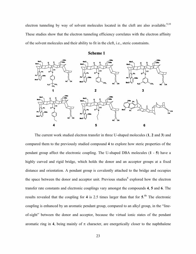
Transcript
Photo-Induced Electron Transfer Studies in Donor-Bridge-Acceptor Molecules
by
Subhasis Chakrabarti
BS, Presidency College, Calcutta University, India, 2000
MS, Indian Institute of Technology, Mumbai, India, 2002
Submitted to the Graduate Faculty of
Arts and Science in partial fulfillment
of the requirements for the degree of
Doctor of Philosophy
University of Pittsburgh
2008
UNIVERSITY OF PITTSBURGH
FACULTY OF ARTS AND SCIENCES
This dissertation was presented
by
Subhasis Chakrabarti
It was defended on
September 8, 2008
and approved by
Dr. David Pratt, Professor, Chemistry
Dr. Sunil Saxena, Professor, Chemistry
Dr. Hyung J. Kim, Professor, Chemistry
Dissertation Advisor: Dr. David H. Waldeck, Professor, Chemistry
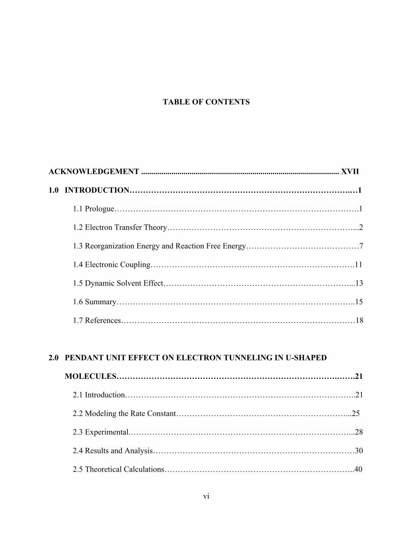
Scheme 1. Kinetic scheme for the forward and backward electron transfer.......................7 Scheme 2. Different U-shaped Donor-Bridge-Acceptor Molecules..................................23 Scheme 3. Different U-shaped molecules..........................................................................59
xvii
ACKNOWLEDGEMENT
I would like to express my deep and sincere gratitude to my supervisor, Professor David H.
Waldeck, Ph.D., Chair of the Department of Chemistry, University of Pittsburgh. His wide
knowledge and his way of thinking towards a scientific problem had a great impact on my
approach towards problem solving. His understanding, encouragements, and personal
guidance have provided a good basis for the present thesis. His constant help and support
from year 2001 (when I was a student in India) until today is something I can not express in
words. I thank him for everything from the core of my heart.
I am deeply grateful to Professor David Pratt for providing me with his valuable comments
and suggestions during my stay in Pittsburgh. He also introduced me to the field of Modern
Quantum Mechanics when I took a course under him in my first year of graduate study.
I owe my most sincere gratitude to Professor Sunil Saxena for his help throughout this study.
He also introduced me to the world of high resolution spectroscopy.
I thank Prof. Kim and Prof. Walker for their support and help.
I thank Professor Alex Star, who gave me the opportunity to work on my proposal under his
guidance. I also thank Prof. Hutchison for his untiring help during my proposal.
xviii
I warmly thank Dr. Min Liu, for her detailed and constructive comments, for her help, and for
her important support when I was a new graduate student and was learning about TCSPC and
electron transfer theory.
During this work I have collaborated with many colleagues for whom I have great regard, and
I wish to extend my warmest thanks to all those who have helped me with my work,
especially Prof. Christian Schafmeister in the Department of Chemistry at the Temple
University and Prof. M. Paddon-Row at the University of South Wales, Australia.
I owe my loving thanks to my fellow group members Lei Wang, Palwinder Kaur, Amit Paul,
Angie Wu, Matt Kofke, Alex Clemens, and Dan Lamont for the lovely moments I had with
them.
I like to thank my family and friends. Without their encouragement and understanding it
would have been impossible for me to finish this work.
I warmly thank the expert staff in the Glass shop, the Electronic shop, and the Machine shop
at University of Pittsburgh for their valuable advice and friendly help.
The financial support from NSF and University of Pittsburgh is gratefully acknowledged.
Pittsburgh, September 2008
Subhasis Chakrabarti
xix
1
1.0 FIRST CHAPTER
1. Introduction
1.1 Prologue
Electron transfer reactions are one of the most fundamental prototype reactions in
science and technology. The modern era of electron transfer reactions started after World War
II with the study of self exchange reactions using isotopes. In 1950, Huang, Rhys and Kubo
advanced a theory of non-radiative transitions of a localized electron from an electronically
excited bound state to the ground electronic state in ionic crystals (in which the electron
transfer is the dominating and central part).1 Their pioneering work first quantitatively
described the nuclear thermally averaged Franck-Condon (FC) vibrational overlap factor in a
single frequency configurational diagram. Later in 1952, Willard Libby described the
significance of nuclear reorganization in electron transfer reactions.2 It was Marcus’ landmark
work, beginning from 1956, that built the foundation for much of what has been learned in the
intervening decades about electron transfer and provided the quantitative description of the
classical high temperature FC factor for outer sphere electron transfer.3,4 In recent years,
scientists have successfully used well-designed Donor-Bridge-Acceptor (DBA) molecules in
order to address the important issues in electron transfer by systematically manipulating the
molecular properties.5,6,7
1.2 Electron transfer theory
1.2.1 Origin and background
Electron transfer involves the movement of an electron from a donor molecule to an
acceptor molecule. A simple example of electron transfer is the self exchange reaction.
Fe2+ + Fe3+↔ Fe3+ + Fe2+ 1
This simple example can be explained easily in terms of Marcus’s classical two parabola
model (two parabolas with same energy). In DBA molecules, the process of electron transfer
is far more complex and we need to use the semiclassical electron transfer theory to describe
the electron transfer process.
The semiclassical electron transfer theory model begins with Fermi’s golden
rule expression for the transition rate.
2
(2 / )k V FCW DS 2
where / 2h ; h = Planck’s constant, V is the electronic coupling matrix element and
FCWDS is the Franck-Condon weighted density of states (thermally averaged vibrational
Franck-Condon factor).8,9 The FCWDS term includes the structural and environmental
variables in the system. This equation satisfies the following conditions.
1. Electron transfer is described as a radiationless process.
2. The Born-Oppenheimer separability of electronic and nuclear motion applies,
allowing for the description of the system in terms of diabatic potential surfaces.
3. The dynamics are described fully by microscopic ET rates which is basically the
non-radiative decay rate of an initial state to the final quasi-degenerate state.
2
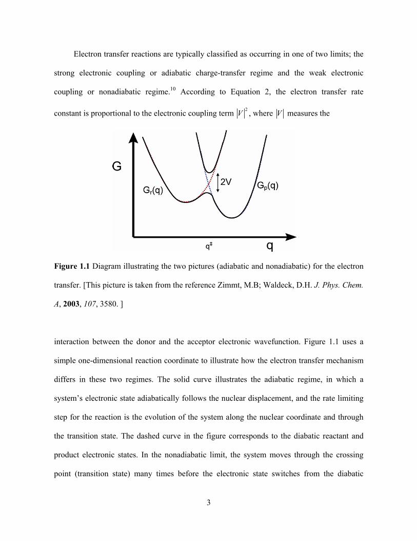
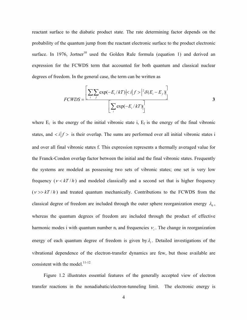
Electron transfer reactions are typically classified as occurring in one of two limits; the
strong electronic coupling or adiabatic charge-transfer regime and the weak electronic
coupling or nonadiabatic regime.10 According to Equation 2, the electron transfer rate
constant is proportional to the electronic coupling term 2
V , where V measures the
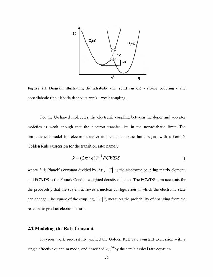
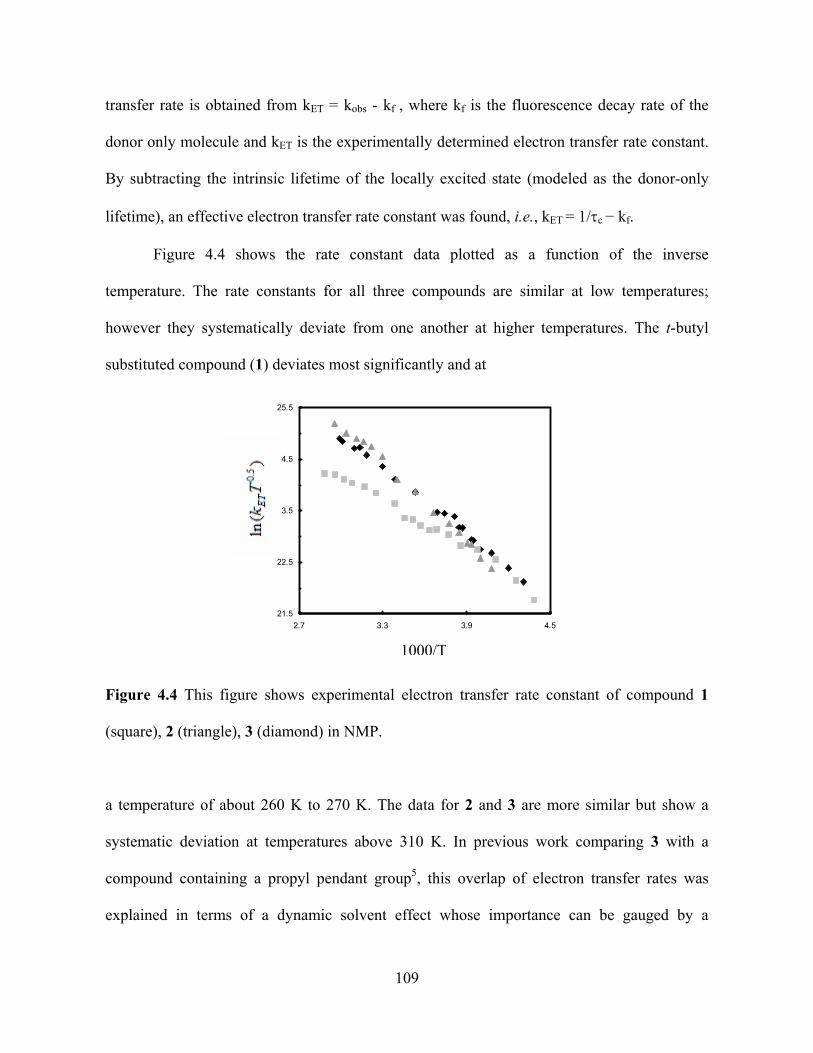
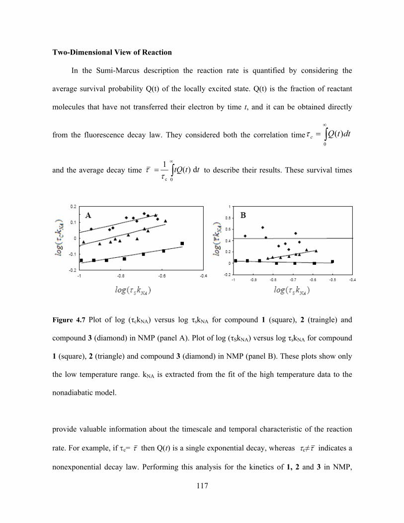
Figure 1.1 Diagram illustrating the two pictures (adiabatic and nonadiabatic) for the electron
transfer. [This picture is taken from the reference Zimmt, M.B; Waldeck, D.H. J. Phys. Chem.
A, 2003, 107, 3580. ]
interaction between the donor and the acceptor electronic wavefunction. Figure 1.1 uses a
simple one-dimensional reaction coordinate to illustrate how the electron transfer mechanism
differs in these two regimes. The solid curve illustrates the adiabatic regime, in which a
system’s electronic state adiabatically follows the nuclear displacement, and the rate limiting
step for the reaction is the evolution of the system along the nuclear coordinate and through
the transition state. The dashed curve in the figure corresponds to the diabatic reactant and
product electronic states. In the nonadiabatic limit, the system moves through the crossing
point (transition state) many times before the electronic state switches from the diabatic
3
reactant surface to the diabatic product state. The rate determining factor depends on the
probability of the quantum jump from the reactant electronic surface to the product electronic
surface. In 1976, Jortner10 used the Golden Rule formula (equation 1) and derived an
expression for the FCWDS term that accounted for both quantum and classical nuclear
degrees of freedom. In the general case, the term can be written as
2exp( / ) ( )
exp( / )
i ii f
ii
E kT i f E E
FCWDS
E kT
f
3
where Ei is the energy of the initial vibronic state i, Ef is the energy of the final vibronic
states, and i f is their overlap. The sums are performed over all initial vibronic states i
and over all final vibronic states f. This expression represents a thermally averaged value for
the Franck-Condon overlap factor between the initial and the final vibronic states. Frequently
the systems are modeled as possessing two sets of vibronic states; one set is very low
frequency ( /kT h ) and modeled classically and a second set that is higher frequency
( /kT h ) and treated quantum mechanically. Contributions to the FCWDS from the
classical degree of freedom are included through the outer sphere reorganization energy 0 ,
whereas the quantum degrees of freedom are included through the product of effective
harmonic modes i with quantum number ni and frequencies i . The change in reorganization
energy of each quantum degree of freedom is given by i . Detailed investigations of the
vibrational dependence of the electron-transfer dynamics are few, but those available are
consistent with the model.11-12
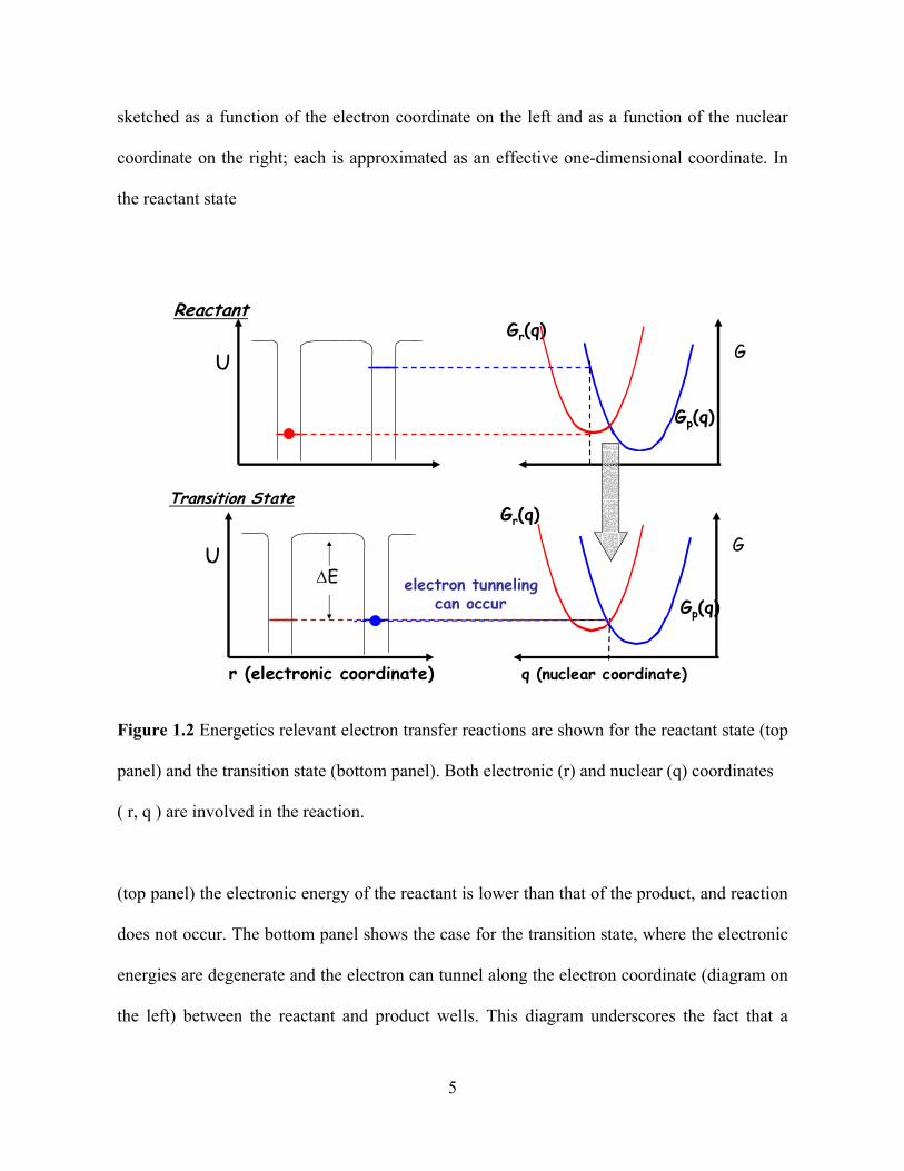
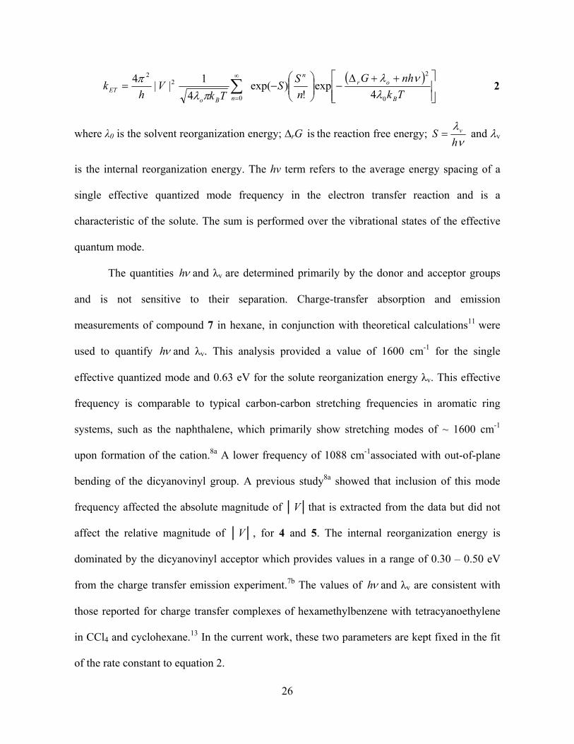
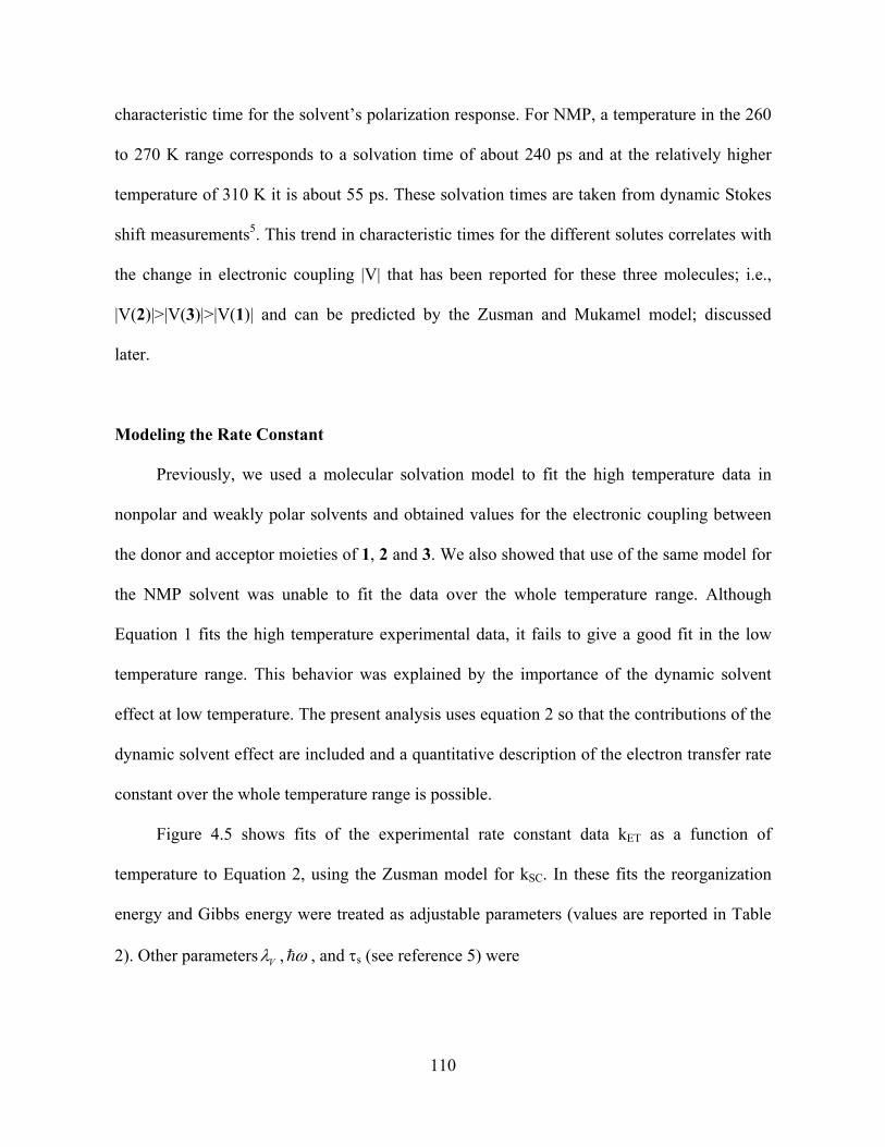
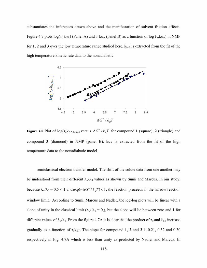
Figure 1.2 illustrates essential features of the generally accepted view of electron
transfer reactions in the nonadiabatic/electron-tunneling limit. The electronic energy is
4
sketched as a function of the electron coordinate on the left and as a function of the nuclear
coordinate on the right; each is approximated as an effective one-dimensional coordinate. In
the reactant state
Reactant
Transition State
Gp(q)
G
q (nuclear coordinate)
Gr(q)
U
r (electronic coordinate)
ΔE
Gp(q)
GGr(q)
U
electron tunnelingcan occur
Figure 1.2 Energetics relevant electron transfer reactions are shown for the reactant state (top
panel) and the transition state (bottom panel). Both electronic (r) and nuclear (q) coordinates
( r, q ) are involved in the reaction.
(top panel) the electronic energy of the reactant is lower than that of the product, and reaction
does not occur. The bottom panel shows the case for the transition state, where the electronic
energies are degenerate and the electron can tunnel along the electron coordinate (diagram on
the left) between the reactant and product wells. This diagram underscores the fact that a
5
successful electron transfer reaction requires motion along the nuclear coordinate(s) to the
transition state and motion along the electronic coordinate from the reactant to the product. If
the electronic interaction between the product and reactant curves at the transition state is
weak enough (pure nonadiabatic limit), the electron transfer rate is controlled by the
electronic motion (tunneling from the reactant to product states). In this limit, the rate
constant kET,NA is given by equation 2. For the DBA molecules studied in this work, a
semiclassical expression, with a single quantized nuclear mode, has been found to provide an
adequate description of the rate constant. In the analysis a coarser representation of the
quantized modes is used. With only one quantum mode, 13 the rate expression becomes
22
2 0
0 00
(4 1exp( ) .exp
! 44
nr
etn BB
G nhSk V S
h nk T
)
k T
4
where is the effective frequency for the quantized vibrational mode, is the reaction
free energy, S is the Huang-Rhys factor
rG
/i h , and the i is the total inner sphere
reorganization energy for all of the relevant modes. The summand n refers to the product’s
vibrational quantum levels. For the systems studied below, the first few terms in the sum over
product vibrational states provide an accurate evaluation of the rate constant, and equation 4
affords a reasonable description of the rate constant.
The electron transfer rate constant predicted by equation 4 is a strong function of the
parameter set used, and an accurate determination of these parameters is necessary when
drawing comparisons with experimental rate data. The quantities h and i are typically
evaluated using a combination of experimental charge-transfer spectra and ab-initio
calculations. Usually, is estimated through experimental redox data and dielectric
continuum corrections to the solvation energy. This approach is not appropriate for weakly
rG
6
polar or non-polar solvents; however, in this study, rG is obtained in non-polar aromatic
solvents from an analysis of the kinetic data using a two-state model (scheme 2).14, 15 This
two- state model assumes that equilibrium exists between the locally excited state and the
charge-separated state and permits the evaluation of the forward and backward electron
transfer rate constants. These data are used to calibrate a molecular-based solvation model
that is able to reproduce experimental ( )rG T values. The same model is used to predict the
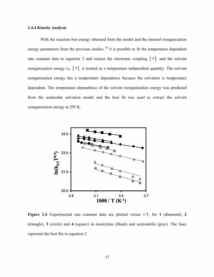
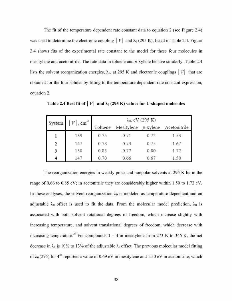
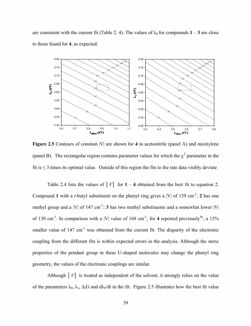
temperature dependence of 0 . The electronic coupling V and 0 (295K) are obtained by
fitting the experimental rate constant data using the rG and 0d
dT
values from the model in
conjunction with i and values (taken from charge transfer spectra of similar molecule).
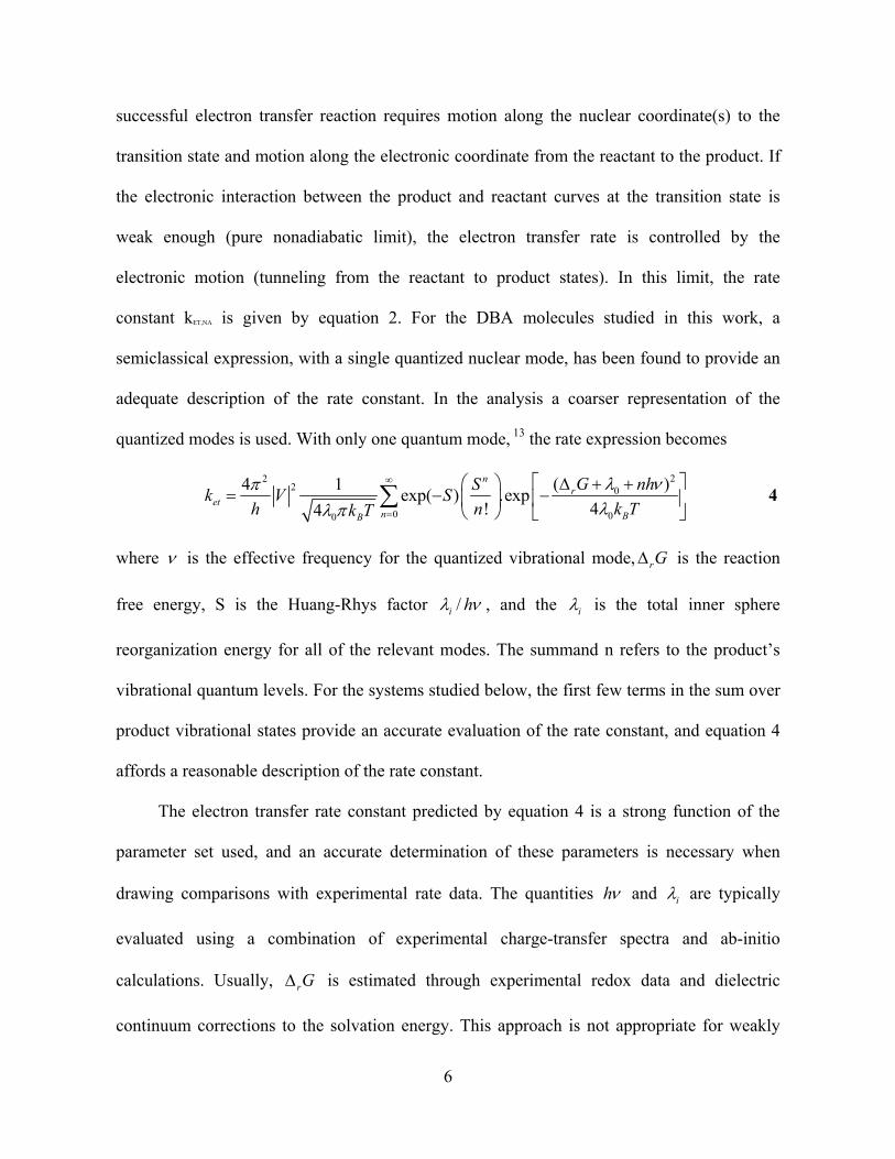
Scheme 1. Kinetic scheme for the forward and backward electron transfer.
1.3 Reorganization energy and reaction free energy
The reorganization energy is a combination of two contributions ( 0V ). V (Internal
reorganization energy) comes from the structural change of the reactant and the product state
from their equilibrium configuration. So V is related to the local changes of the geometry of
7
the reactant and the product state during electron transfer. In a single–mode semiclassical
expression, the interaction with the solvent is modeled classically and the solute vibrations
which are expressed as a single effective high-frequency mode are modeled quantum
mechanically. Previous studies have shown that the internal reorganization energy V and the
effective mode frequency do not have a significant solvent dependence. For typical organic
DBA systems (the molecules used for this study), one finds that the characteristic vibrational
frequencies in the range of 1400-1600 cm-1 constitute a major fraction of the reorganization
energy changes in the high frequency modes. This reflects the changes in the carbon-carbon
bond lengths in these aromatic molecules during electron transfer. From charge transfer
spectra (if available) and quantum chemistry calculations one can quantify the high frequency
mode parameters. For systems in which charge transfer spectra are detected, free energy and
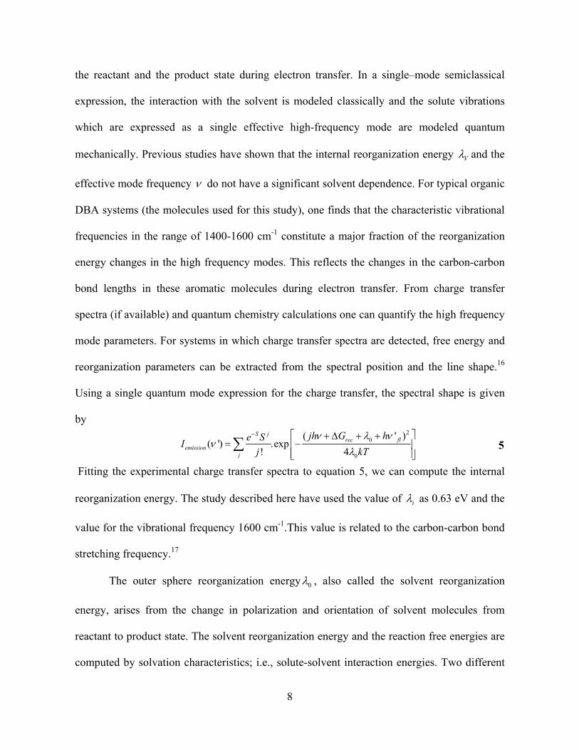
reorganization parameters can be extracted from the spectral position and the line shape.16
Using a single quantum mode expression for the charge transfer, the spectral shape is given
by
5 2
0( ') .exp! 4
rec flemission
e SI
j kT
0
( ' )S j
j
jh G h
Fitting the experimental charge transfer spectra to equation 5, we can compute the internal
reorganization energy. The study described here have used the value of i as 0.63 eV and the
value for the vibrational frequency 1600 cm-1.This value is related to the carbon-carbon bond
stretching frequency.17
The outer sphere reorganization energy 0 , also called the solvent reorganization
energy, arises from the change in polarization and orientation of solvent molecules from
reactant to product state. The solvent reorganization energy and the reaction free energies are
computed by solvation characteristics; i.e., solute-solvent interaction energies. Two different
8
models can be used to treat the solute-solvent interactions; a dielectric continuum model and a
molecular solvation model. The simple dielectric continuum model calculates solvation
energies using a static dielectric constant S and a high-frequency dielectric constant .18-20
The solute is treated as a spherical (or even ellipsoidal) cavity containing a point source. In
the case of bimolecular reactions, the model includes two spherical cavities, each containing a
point charge, whereas for intramolecular electron transfer reactions, it is more convenient to
consider the solute as a cavity having a permanent dipole moment.
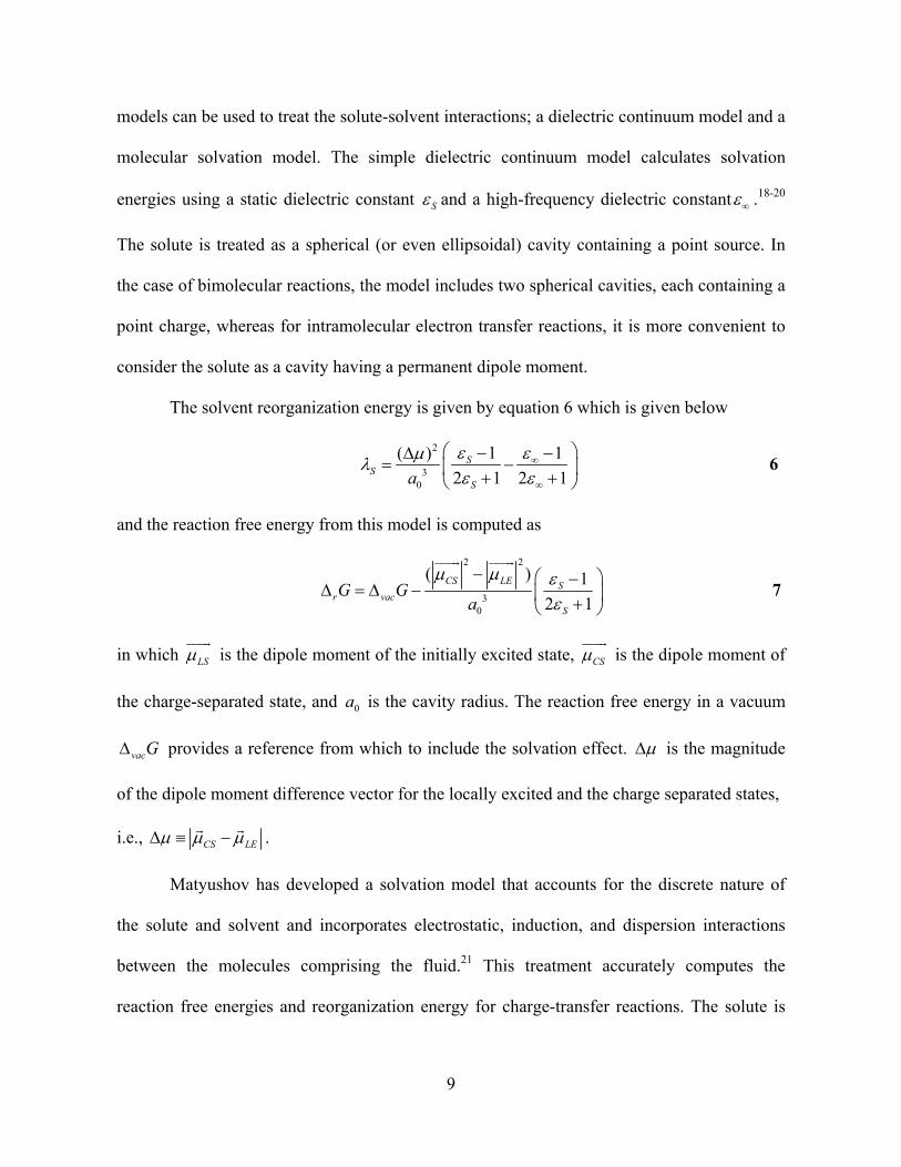
The solvent reorganization energy is given by equation 6 which is given below
2
30
( )
1 1
2 1 2 1S
SSa
6
and the reaction free energy from this model is computed as
2 2
30
( ) 1
2 1
CS LE Sr vac
S
G Ga
7
in which LS
is the dipole moment of the initially excited state, CS
is the dipole moment of
the charge-separated state, and is the cavity radius. The reaction free energy in a vacuum
provides a reference from which to include the solvation effect.
0a
vacG is the magnitude
of the dipole moment difference vector for the locally excited and the charge separated states,
i.e., CS LE
.
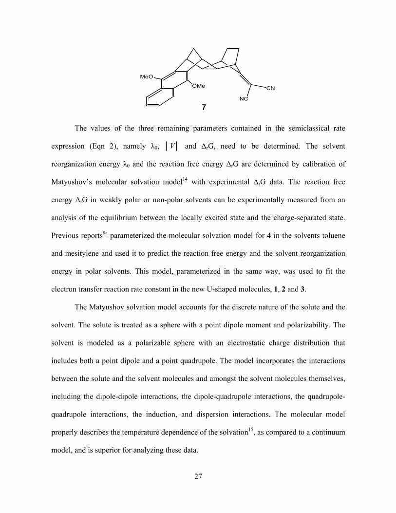
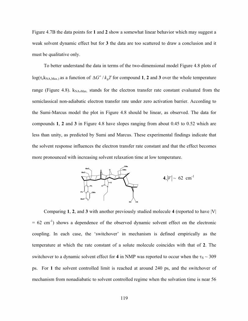
Matyushov has developed a solvation model that accounts for the discrete nature of
the solute and solvent and incorporates electrostatic, induction, and dispersion interactions
between the molecules comprising the fluid.21 This treatment accurately computes the
reaction free energies and reorganization energy for charge-transfer reactions. The solute is
9
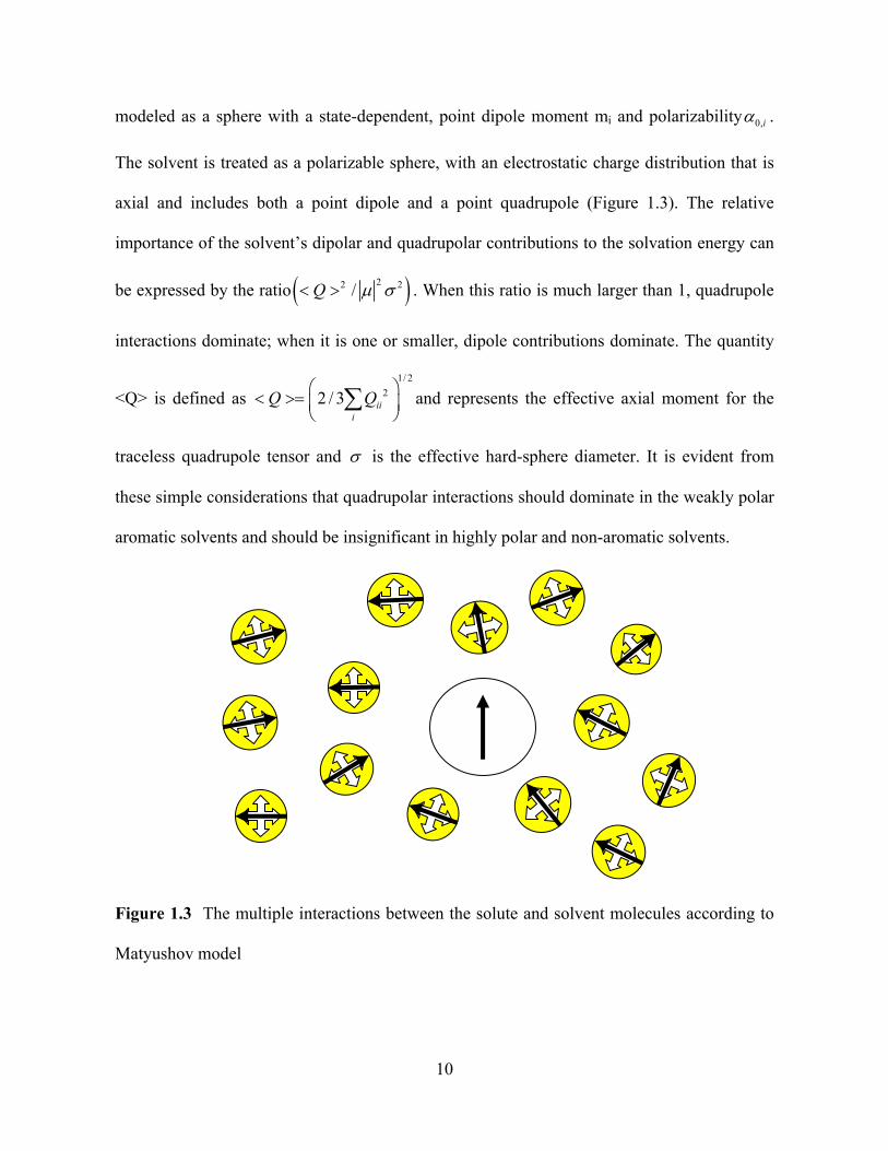
modeled as a sphere with a state-dependent, point dipole moment mi and polarizability 0,i .
The solvent is treated as a polarizable sphere, with an electrostatic charge distribution that is
axial and includes both a point dipole and a point quadrupole (Figure 1.3). The relative
importance of the solvent’s dipolar and quadrupolar contributions to the solvation energy can
be expressed by the ratio 22 /Q 2 . When this ratio is much larger than 1, quadrupole
interactions dominate; when it is one or smaller, dipole contributions dominate. The quantity
<Q> is defined as and represents the effective axial moment for the
traceless quadrupole tensor and
1/ 2
22 / 3 iii
Q Q
is the effective hard-sphere diameter. It is evident from
these simple considerations that quadrupolar interactions should dominate in the weakly polar
aromatic solvents and should be insignificant in highly polar and non-aromatic solvents.
Figure 1.3 The multiple interactions between the solute and solvent molecules according to
Matyushov model
10
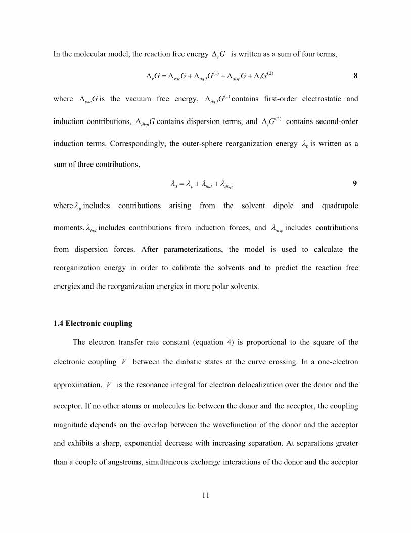
In the molecular model, the reaction free energy rG is written as a sum of four terms,
8 (1) (2),r vac dq i disp iG G G G G
where is the vacuum free energy, contains first-order electrostatic and
induction contributions, contains dispersion terms, and contains second-order
induction terms. Correspondingly, the outer-sphere reorganization energy
vacG (1),dq iG
dispG (2)iG
0 is written as a
sum of three contributions,
0 p ind disp 9
where p includes contributions arising from the solvent dipole and quadrupole
moments, ind includes contributions from induction forces, and disp includes contributions
from dispersion forces. After parameterizations, the model is used to calculate the
reorganization energy in order to calibrate the solvents and to predict the reaction free
energies and the reorganization energies in more polar solvents.
1.4 Electronic coupling
The electron transfer rate constant (equation 4) is proportional to the square of the
electronic coupling V between the diabatic states at the curve crossing. In a one-electron
approximation, V is the resonance integral for electron delocalization over the donor and the
acceptor. If no other atoms or molecules lie between the donor and the acceptor, the coupling
magnitude depends on the overlap between the wavefunction of the donor and the acceptor
and exhibits a sharp, exponential decrease with increasing separation. At separations greater
than a couple of angstroms, simultaneous exchange interactions of the donor and the acceptor
11
with the intervening pendant group (non-bonded contact), or inclusion of the solvent molecule
in the cleft, mediates the electronic coupling, generating larger interaction energies than the
direct exchange interaction. In the U-shaped DBA molecules the electronic coupling is found
to be solvent independent. The rotation and conformation of the intervening pendant group
can also affect the magnitude of the electronic coupling.
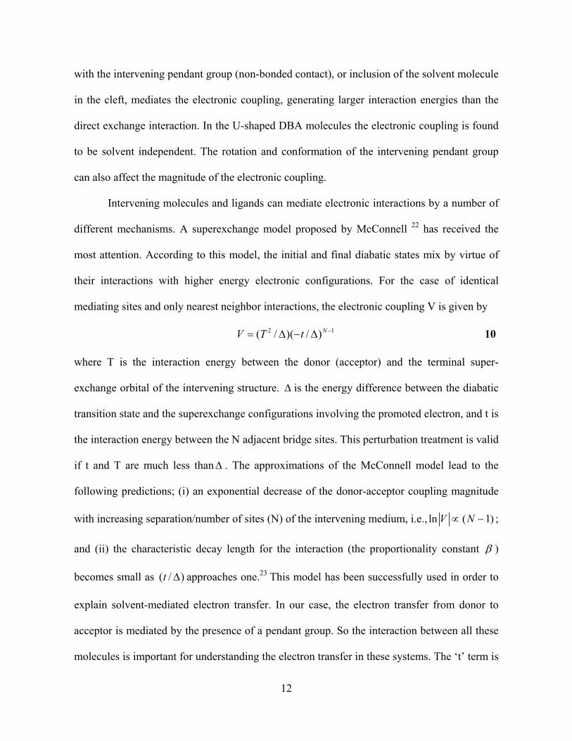
Intervening molecules and ligands can mediate electronic interactions by a number of
different mechanisms. A superexchange model proposed by McConnell 22 has received the
most attention. According to this model, the initial and final diabatic states mix by virtue of
their interactions with higher energy electronic configurations. For the case of identical
mediating sites and only nearest neighbor interactions, the electronic coupling V is given by
2( / )( / )NV T t 1 10
where T is the interaction energy between the donor (acceptor) and the terminal super-
exchange orbital of the intervening structure. is the energy difference between the diabatic
transition state and the superexchange configurations involving the promoted electron, and t is
the interaction energy between the N adjacent bridge sites. This perturbation treatment is valid
if t and T are much less than . The approximations of the McConnell model lead to the
following predictions; (i) an exponential decrease of the donor-acceptor coupling magnitude
with increasing separation/number of sites (N) of the intervening medium, i.e.,
ln ( 1)V N ;
and (ii) the characteristic decay length for the interaction (the proportionality constant )
becomes small as ( / approaches one.23 This model has been successfully used in order to
explain solvent-mediated electron transfer. In our case, the electron transfer from donor to
acceptor is mediated by the presence of a pendant group. So the interaction between all these
molecules is important for understanding the electron transfer in these systems. The ‘t’ term is
)t
12
not important here as the electron tunnels through the non-covalent contacts (through space),
not through the bridge. So the magnitude of the term t/Δ is very low. At the same time the
value of N reduced to unity as there will be one pendant molecule between donor and
acceptor and the size, rotation and the orientation of the pendant molecule plays an important
role in the electronic coupling. Hence, for fixed donor-spacer-acceptor molecules, different
pendant groups can modulate the electronic coupling.
1.5 Dynamic Solvent Effect
A solvent molecule can change the energetics of the electron transfer reaction either
by interacting with the reactant and product or by actively participating in the reaction in a
more dynamic way by exchanging energy and momentum with reacting species. This effect is
known as a solvent dynamic effect. Dynamic solvent effects are mainly associated with the
dielectric friction of the polar solvents. These dynamical features of polar interactions can
play an important role in determining the electron transfer reaction rates. The molecular
mechanism of dynamic solvation can be viewed as the reorientation of dipolar solvent
molecules around the solute molecules due to the newly distributed charge of a solute. The
more polar the solvent, the stronger is the coupling between the molecules. The polarization
responses also depend on the intermolecular solvent interactions. Zusman24 first considered
this effect, which has since been studied by several other groups.25-30
One approach to study solvation dynamic effects are “continuum” models.31-36 These
models treat the solute as a point dipole in a spherical cavity that is immersed in solvent
which is treated as a continuum, frequency-dependent dielectric. Simple continuum models
13
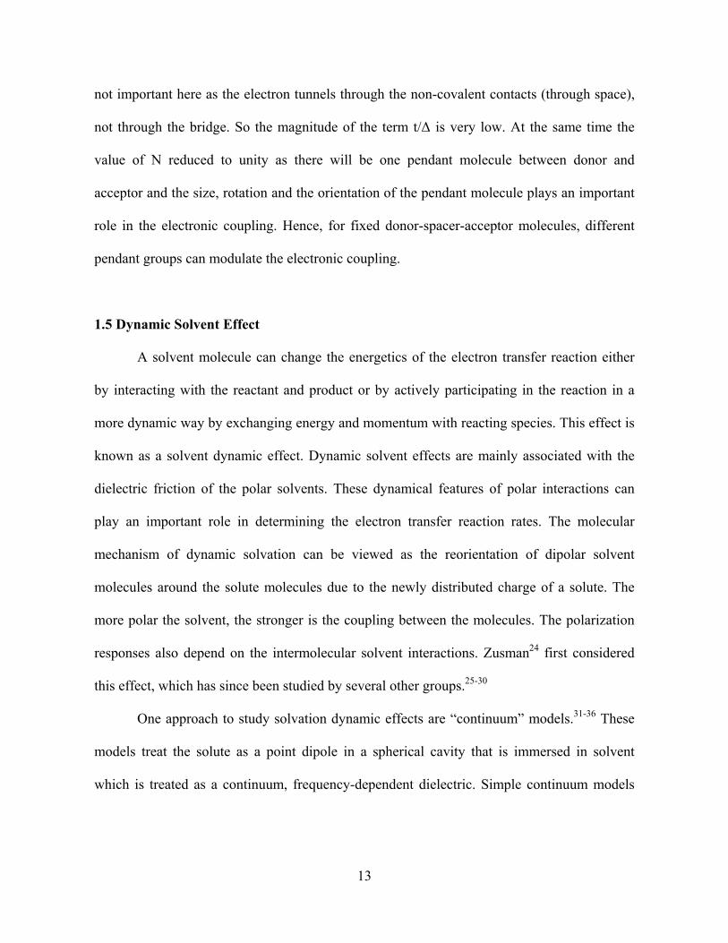
predict that the solvent has an exponential solvation response function, given by the following
equation
)/exp()( LttS 11
The dynamic solvation time is equal to the longitudinal relaxation time ( L ) of the solvent
0
DL 12
where ε0 is the static dielectric constant, is the high-frequency dielectric constant, and D
is the dielectric (or Debye) relaxation time.
In intramolecular electron transfer reactions, when the electron tunneling rate is much
faster than the reorientation time of the solvent, then the solvent reorientation can become the
rate limiting step of the reaction. In this case, the electron transfer rate is limited by the
relaxation rate of the solvent and the reaction is a solvent-controlled electron transfer reaction.
In contrast, when the solvent reorientation rate is much faster than the electron transfer rate,
the relaxation time of solvent has no effect on the electron transfer and it is a nonadiabatic
electron transfer reaction.
For non Debye solvents, which are characterized by more than one relaxation time
scale, people have used the correlation time of the solvent relaxation which is defined as
0
( )S t dt
13
This correlation time is a measure of the solvation time.
14
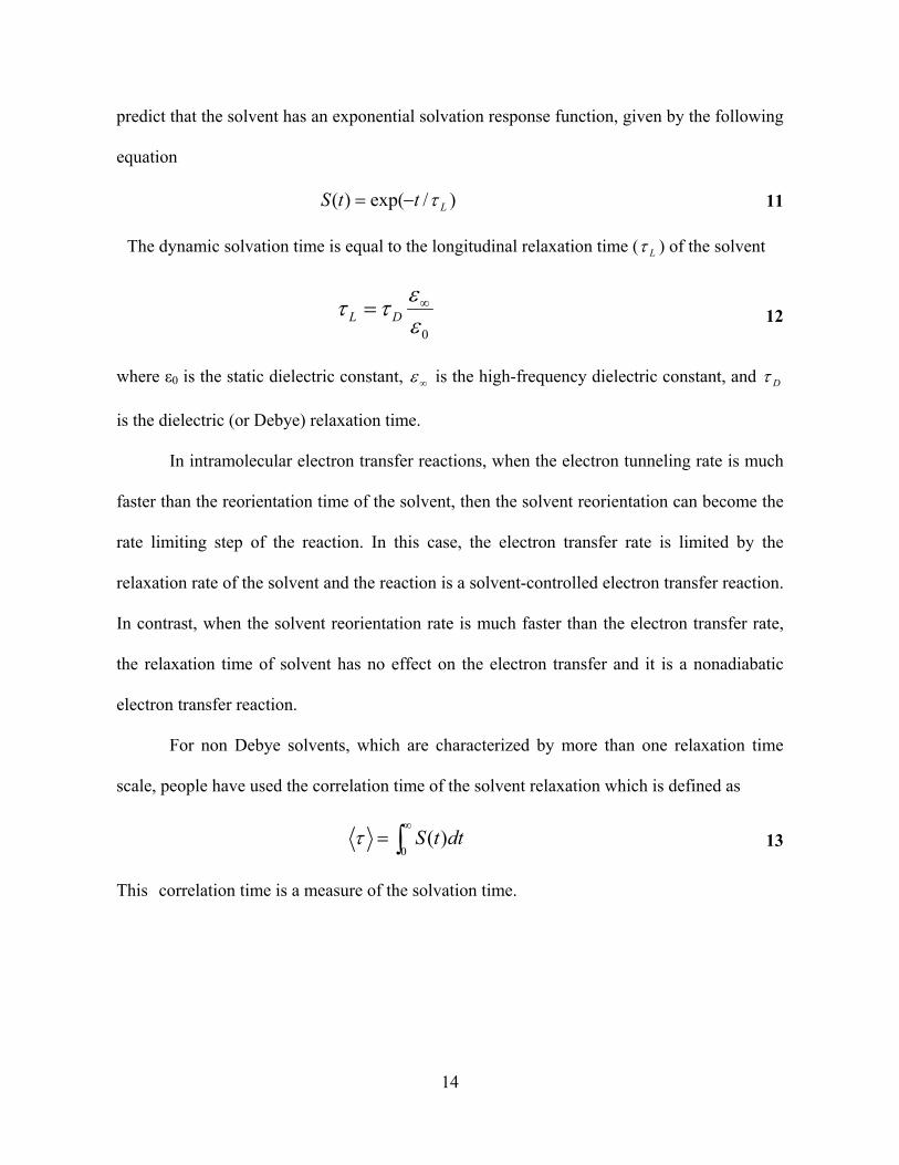
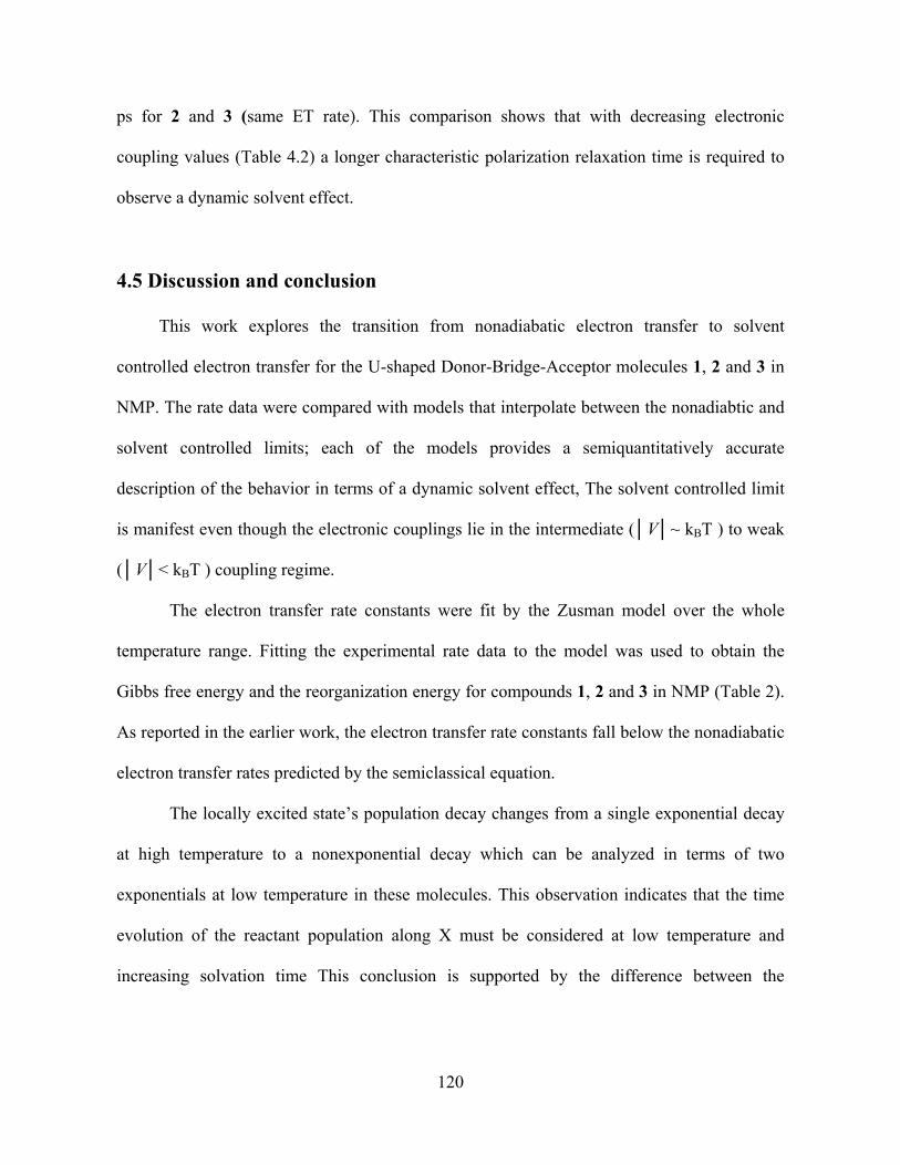
1.6 Summary
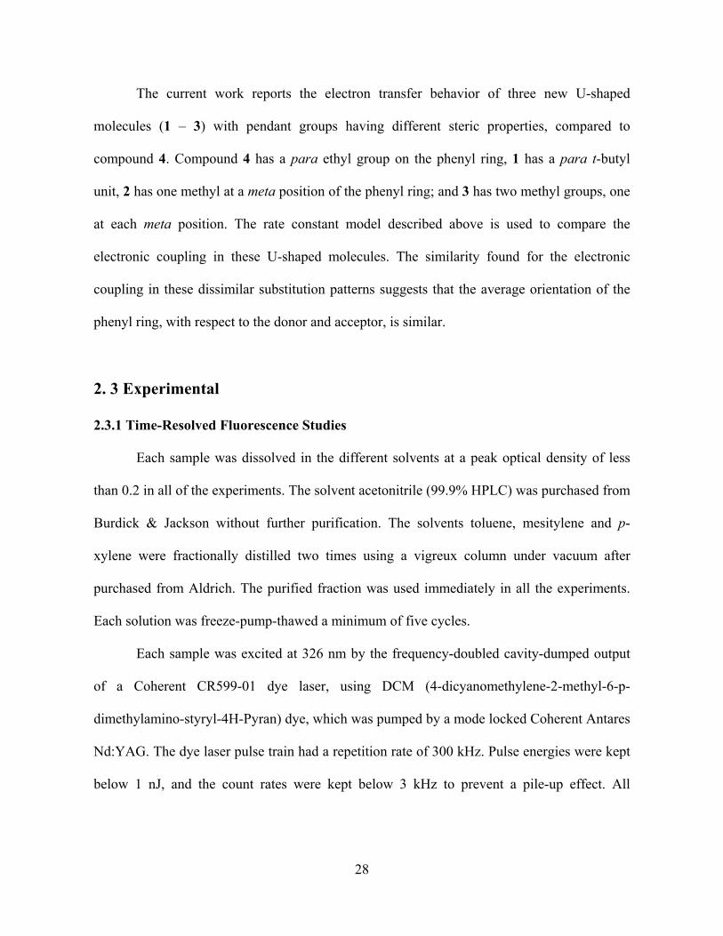
This thesis probes the electron transfer mechanism and kinetics in different DBA
molecular systems in detail. Chapter 2 and 3 use different U-shaped Donor-Bridge-Acceptor
molecules to illustrate how the electron transfer mechanism and kinetics depends on the
nature of the pendant unit present in the “line of sight” between the donor and acceptor
moieties (Figure 1.4). The experimental results are compared with the semiclassical equation
and molecular solvation model. The results prove that the electronic coupling depends on the
nature of the substituent groups on the phenyl ring present in the cavity. Electron
O O
NC CN
OMeOMeMeO
MeO
NOO
CH3
Ph
Ph OMe
MeO
H3CCH3
O O
NC CN
OMe
OMeMeO
MeO
NOO
Ph
Ph OMe
MeO
O O
NC CN
OMeOMeMeO
MeO
NOO
Ph
Ph OMe
MeOCH3
O O
NC CN
OMe
OMeMeO
MeO
NOO
Ph
Ph OMe
MeOH3C CH3
O O
NC CN
OMeOMeMeO
MeO
NOO
Ph
Ph OMe
MeO
OMe
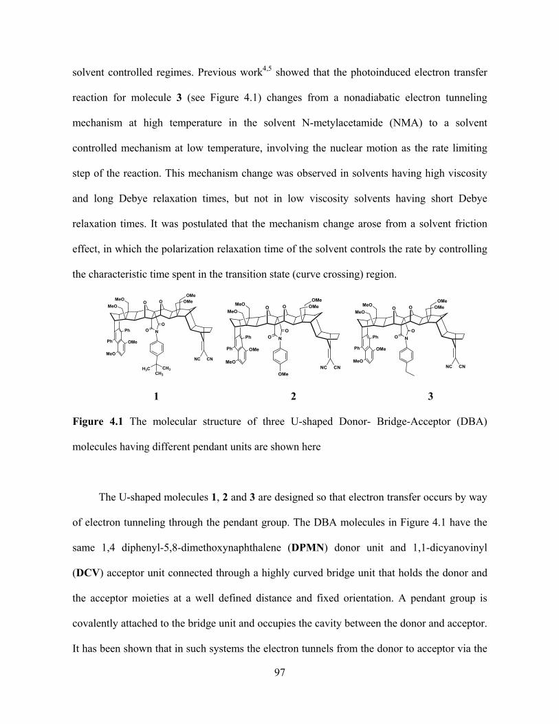
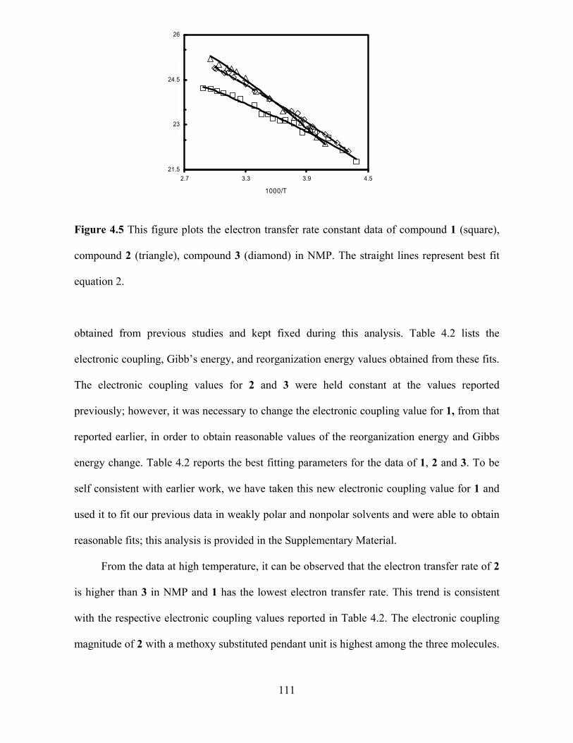
Figure 1.4 U-shaped Donor-Bridge-Acceptor molecules studied in chapter 2, 3 and 4
donating groups present in the aromatic ring do not change the electronic coupling values
whereas the presence of electron withdrawing groups present in the ring can enhance the
electronic coupling a lot and hence the electron transfer rate. Chapter 4 demonstrates that a
switchover of electron transfer mechanism occur from a nonadiabatic electron transfer
15
towards an “adiabatic” electron transfer in highly viscous and slowly relaxing solvent NMP.
The experimental results were analyzed in terms of different theoretical models to explain the
dynamic solvent effect observed in our system.
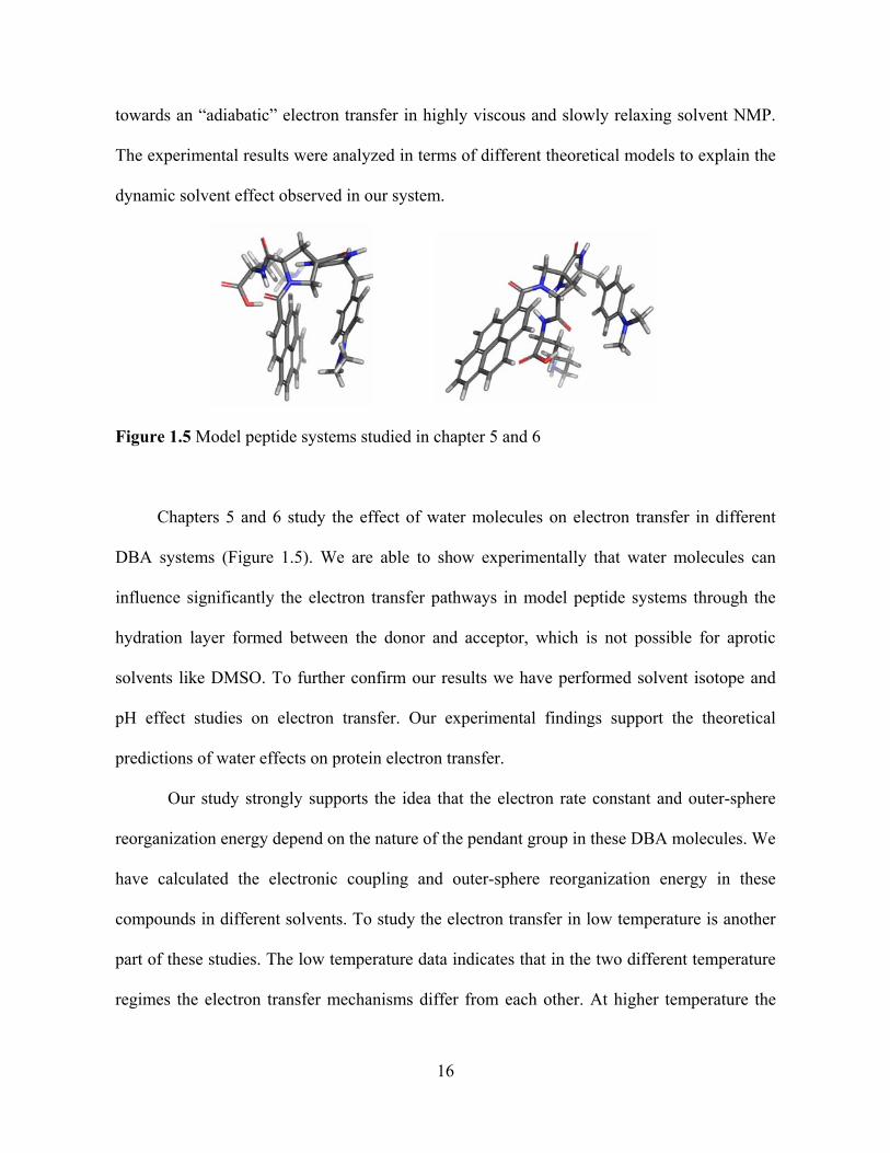
Figure 1.5 Model peptide systems studied in chapter 5 and 6
Chapters 5 and 6 study the effect of water molecules on electron transfer in different
DBA systems (Figure 1.5). We are able to show experimentally that water molecules can
influence significantly the electron transfer pathways in model peptide systems through the
hydration layer formed between the donor and acceptor, which is not possible for aprotic
solvents like DMSO. To further confirm our results we have performed solvent isotope and
pH effect studies on electron transfer. Our experimental findings support the theoretical
predictions of water effects on protein electron transfer.
Our study strongly supports the idea that the electron rate constant and outer-sphere
reorganization energy depend on the nature of the pendant group in these DBA molecules. We
have calculated the electronic coupling and outer-sphere reorganization energy in these
compounds in different solvents. To study the electron transfer in low temperature is another
part of these studies. The low temperature data indicates that in the two different temperature
regimes the electron transfer mechanisms differ from each other. At higher temperature the
16
electronic tunneling mechanism dominates and at lower temperature the rate is limited by
solvent dynamical effects. The last part of this thesis studies how water molecules affect the
electron transfer kinetics. The results show that water molecules can greatly influence the
electron transfer rate.
17
1.7 References
1. Bixon, M.; Jortner, J. Adv. Chem. Phys. 1999, 106, 35.
2. Libby, W. F. J. Phys. Chem. 1952, 56, 863.
3. Marcus, R. A. J. Chem. Phys. 1956, 24, 966.
4. (a) Zimmt, M. B.; Waldeck, D. H. J. Phys. Chem. A. 2003, 107, 3850.(b) Paddon- Row,
M. N. Acc. Chem. Res. 1994, 27, 18. (c) Balzani, V., Ed. Electron Transfer in Chemistry,
Vol. 3; Wiley-VCH: Weinhein, 2001. (d) Johnson, M. D.; Miller, J. R.; Green, N. S.;
Closs, G. L. J. Phys. Chem. 1989, 93, 1173.
5. (a) Zeng, Y.; Zimmt, M. B. J. Phys. Chem. 1992, 96, 8395. (b) Oliver, A. M.; Paddon-
Row, M. N.; Kroon, J.; Verhoeven, J. W. Chem. Phys. Lett. 1992, 191, 371.
6. Closs, G. L.; Miller, J. R. Science 1988, 240, 440.
7. Zener, C. Proc. R. Lond. A. 1932, 137, 969.
8. Landau, L. Phys. Z. Sowj. U. 1932, 1, 88.
9. (a) Zusman, L. D. Z. Phys. Chem. 1994, 186, 1. (b) Onuchic, J. N.; Beratan, D. N.;
Hopfield, J. J. J. Phys. Chem. 1986, 90, 3707.
10. Jortner, J. J. Chem. Phys. 1976, 64, 4860.
11. (a) Kelly, A. M. J. Phys. Chem. A. 1999, 103, 6891. (b) Wang, C.; Mohney, B. K.;
Williams, R.; Hupp, J. T.; Walker, G. C. J. Am. Chem. Soc. 1998, 120, 5848 (c) Markel,
F.; Ferris, N. S.; Gould, I. R.; Myers, A. B. J. Am. Chem. Soc. 1992, 114, 6208.
12. Barbara, P. F.; Meyer, T. J.; Ratner, M. A. J. Phys. Chem. 1996, 100, 13148.
13. Gu, Y.; Kumar, K.; Lin, Z.; Read, I.; Zimmat, M. B.; Waldeck, D. J. Photochem.
Photobiol. A. 1997, 105, 189.
18
14. Read, I.; Napper, A.; Kaplan, R.; Zimmat, M. B.; Waldeck, D.H. J. Am. Chem. Soc. 1999,
121, 10976.
15. (a) Marcus, R. A. J. Phys. Chem. 1989, 93, 3078. (b) Cortes, J.; Heitele, H.; Jortner, J. J.
Phys. Chem. 1994, 98, 2527.
16. Napper, A. M.; Head, N. J.; Oliver, A. M.; Shephard, M. J.; Paddon-Row, M. N.; Read, I.;
Waldeck, D. H. J. Am. Chem. Soc. 2002, 124, 10171,
17. Newton, M. D.; Basilevsky, M. V.; Rostov, I. V. Chem. Phys. 1998, 232, 201.
Komaromi, I.; Martin, R. L.; Fox, D. J.; Keith, T.; Al-Laham, M. A.; Peng, C. Y.;
Nanayakkara, A.; Challacombe, M.; Gill, P. M. W.; Johnson, B.; Chen, W.; Wong, M.
W.; Gonzalez, C.; Pople, J. A. Gaussian, Inc., Pittsburgh PA, 2003
25. Rothenfluh, D. F.; Paddon-Row, M. N. J. Chem. Soc. Perkin Trans. 1996, 2, 639.
26. Jordan, K. D.; Michejda, J. A.; Burrow, P. D. J. Am. Chem. Soc. 1976, 98, 1295.
27. a) Napper, A. M.; Read, I.; Kaplan, R.; Zimmt, M. B.; Waldeck, D. H. J. Phys. Chem. A.
2002, 106, 5288.b) Kaplan, R.; Napper, A. M.; Waldeck, D. H.; Zimmt, M. B. J. Phys.
Chem. A. 2002, 106, 1917.
28. Koeberg, M.; de Groot, M.; Verhoeven, J. W.; Lokan, N. R.; Shephard, M. J.; Paddon-
Row, M. N. J. Phys. Chem. A. 2001, 105, 3417. b) Goes, M. de Groot, M.; Koeberg, M.;
Verhoeven, J. W.; Lokan, N. R.; Shephard, M. J.; Paddon-Row, M. N. J. Phys. Chem. A.
2002, 106 , 2129.
55
3.0 CHAPTER THREE
Competing Electron Transfer Pathways in Hydrocarbon Frameworks:
Short-Circuiting Through-Bond Coupling by Non-Bonded Contacts in
Rigid U-Shaped Norbornylogous Systems Containing a Cavity-Bound
Aromatic Pendant Group
This work has been published as S. Chakrabarti, D. H. Waldeck, A. M. Oliver, and M.
Paddon-Row J. Am. Chem. Soc. 2007, 129, 3247-3256
This work explores electron transfer through non-bonded contacts in two U-shaped DBA
molecules 1DBA and 2DBA by measuring electron transfer rates in organic solvents of
different polarities. These molecules have identical U-shaped norbornylogous frameworks,
twelve bonds in length and with diphenyldimethoxynaphthalene (DPMN) donor and
dicyanovinyl (DCV) acceptor groups fused at the ends. The U-shaped cavity of each molecule
contains an aromatic pendant group of different electronic character, namely p-ethylphenyl, in
1DBA, and p-methoxyphenyl, in 2DBA. Electronic coupling matrix elements, Gibbs free
energy, and reorganization energy were calculated from experimental photophysical data for
these compounds, and the experimental results were compared with computational values.
56
The magnitude of the electronic coupling for photoinduced charge separation, CSV , in 1DBA
and 2DBA were found to be 147 and 274 cm-1, respectively, and suggests that the origin of
this difference lies in the electronic nature of the pendant aromatic group and charge
separation occurs by tunneling through the pendant group, rather than through the bridge.
2DBA, but not 1DBA, displayed charge transfer (CT) fluorescence in nonpolar and weakly
polar solvents and this observation enabled the electronic coupling for charge recombination,
CRV , in 2DBA to be made, the magnitude of which is ~ 500 cm-1, significantly larger than
that for charge separation. This difference is explained by changes in the geometry of the
molecule in the relevant states; because of electrostatic effects, the donor and acceptor
chromophores are about 1Å closer to the pendant group in the charge-separated state than in
the locally excited state. Consequently the through-pendant-group electronic coupling is
stronger in the charge-separated state – which controls the CT fluorescence process – than in
the locally excited state – which controls the charge separation process. The magnitude of
CRV for 2DBA is almost two orders of magnitude greater than that in DMN-12-DCV, having
the same length bridge as for the former molecule, but lacking a pendant group. This result
unequivocally demonstrates the operation of the through-pendant-group mechanism of
electron transfer in the pendant-containing U-shaped systems of the type 1DBA and 2DBA.
3.1 Introduction
Electron transfer reactions are a fundamental reaction type and are of intrinsic
importance in biology, chemistry and the emerging field of nanoscience.1 Donor-Bridge-
Acceptor (DBA) molecules allow systematic manipulation of the molecular properties2,3,4 and
provide an avenue to address important fundamental issues in electron transfer. For example,
57
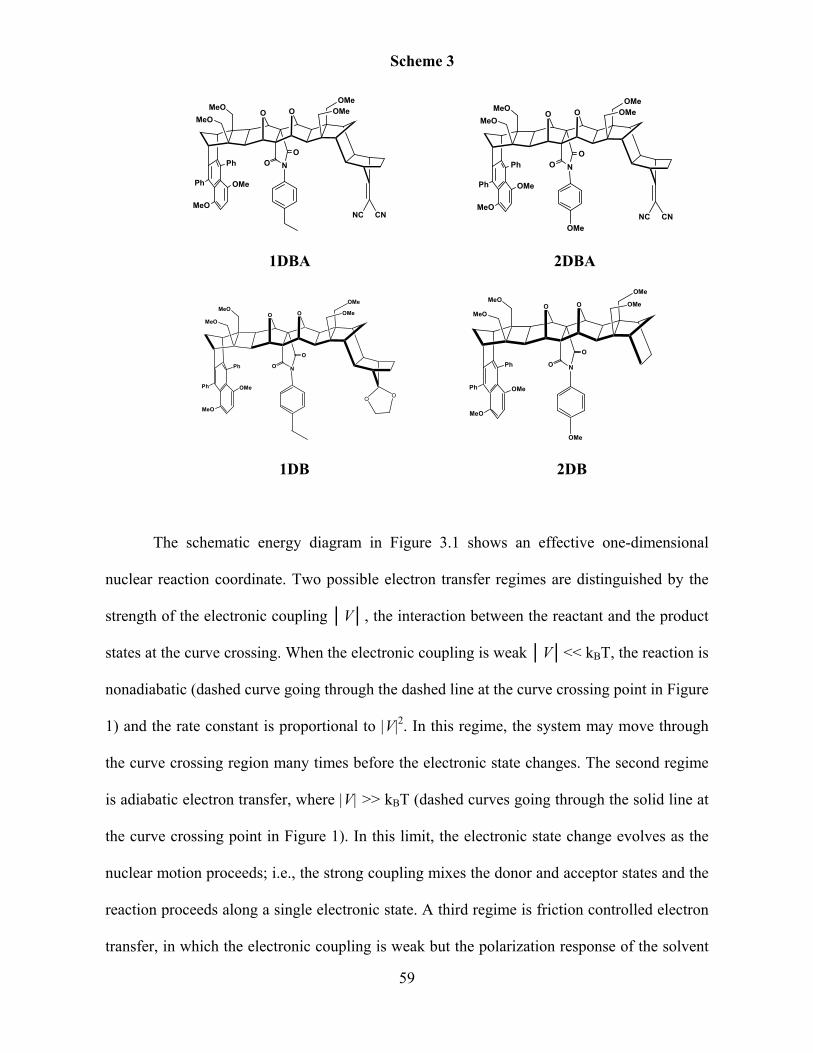
the U-shaped DBA molecules (in Scheme 1) hold the donor and the acceptor units at a fixed
distance and conformation by a rigid hydrocarbon bridge and allow one to study the electron
tunneling over a 5 to 10 angstrom distance scale. Placement of a pendant group in the cleft
changes the electronic tunneling probability (electronic coupling magnitude) between the
donor and acceptor, thereby changing the electron transfer rate. Previous work has shown that
using an aromatic group as a pendant unit increases the electron tunneling probability, as
compared to an aliphatic pendant,5 but that different alkyl substituted phenyl groups have
similar electronic couplings.6
The current work investigates the photoinduced electron transfer kinetics and charge-
transfer emission spectra of the U-shaped DBA molecule 2DBA, bearing a p-methoxyphenyl
pendant group in different aromatic solvents, and compares it with the previously studied
molecule 1DBA, having an ethyl substituted phenyl group (Scheme 1). This allows us to
explore how the electronic nature of the pendant group affects the electronic coupling. The
molecules 1DBA and 2DBA have the same 1,4 diphenyl-5,8-dimethoxynaphthalene (DPMN)
donor unit and 1,1-dicyanovinyl (DCV) acceptor unit connected through a highly curved
bridge unit which holds the donor and the acceptor moieties at a particular distance and
orientation. A pendant group is covalently attached to the bridge and occupies the space
between the donor and the acceptor. It has been shown that the electron tunnels from the
donor to the acceptor unit through the “ line-of-sight ” noncovalent linkage between the donor
and the acceptor.7 It has been established that the electron transfer mechanism in 1DBA is
non-adiabatic at high temperature and in solvents with rapid solvation responses. In this
mechanistic limit, the electron tunneling probability is proportional to the square of the
electronic coupling,2
V .
58
O O
NC CN
OMeOMeMeO
MeO
NOO
Ph
Ph OMe
MeO
O O
NC CN
OMeOMeMeO
MeO
NOO
Ph
Ph OMe
MeO
OMe
1DBA 2DBA
O O
OMe
OMeMeO
MeO
NO
O
Ph
Ph OMe
MeO
OO
O O
OMe
OMeMeO
MeO
NO
O
Ph
Ph OMe
MeO
OMe
1DB 2DB
Scheme 3
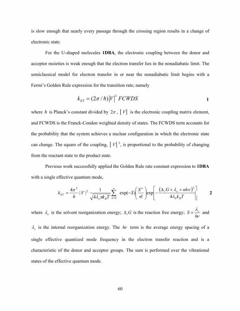
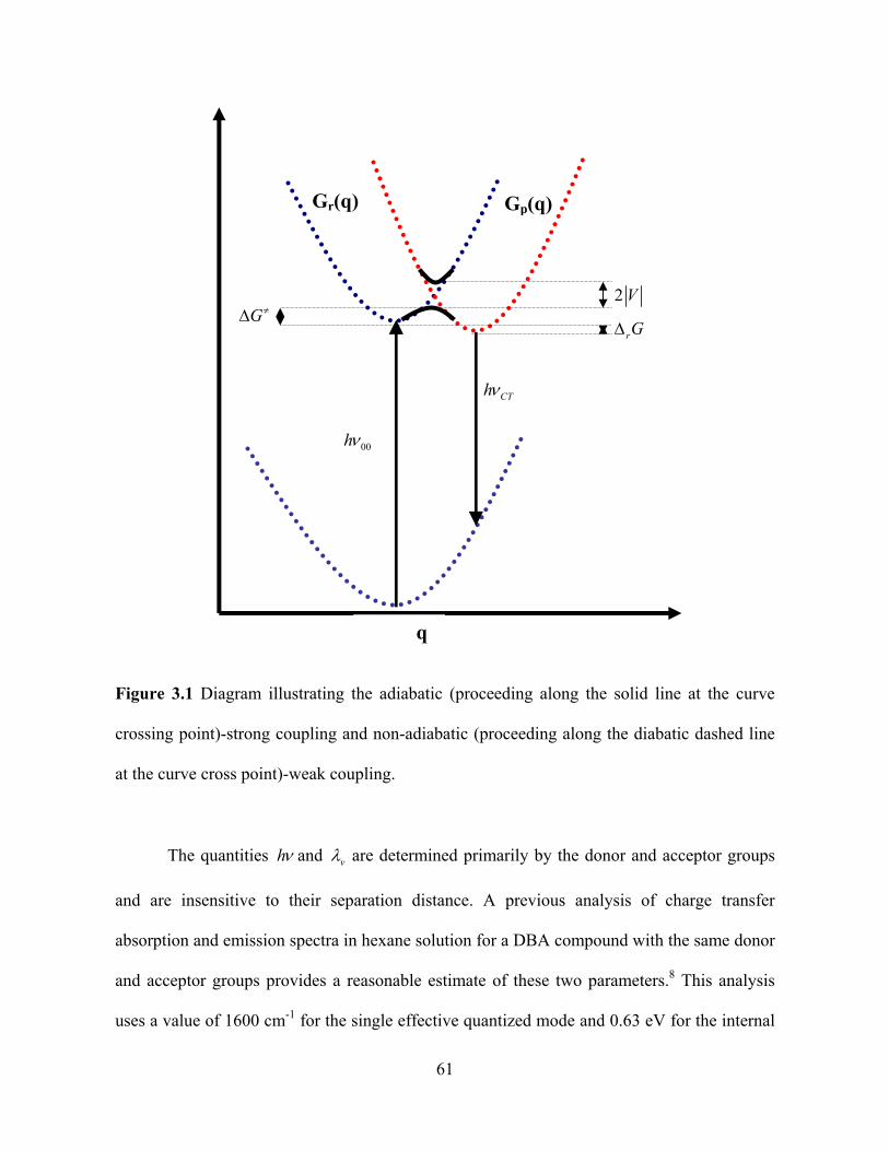
The schematic energy diagram in Figure 3.1 shows an effective one-dimensional
nuclear reaction coordinate. Two possible electron transfer regimes are distinguished by the
strength of the electronic coupling │V│, the interaction between the reactant and the product
states at the curve crossing. When the electronic coupling is weak │V│<< kBT, the reaction is
nonadiabatic (dashed curve going through the dashed line at the curve crossing point in Figure
1) and the rate constant is proportional to |V|2. In this regime, the system may move through
the curve crossing region many times before the electronic state changes. The second regime
is adiabatic electron transfer, where |V| >> kBT (dashed curves going through the solid line at
the curve crossing point in Figure 1). In this limit, the electronic state change evolves as the
nuclear motion proceeds; i.e., the strong coupling mixes the donor and acceptor states and the
reaction proceeds along a single electronic state. A third regime is friction controlled electron
transfer, in which the electronic coupling is weak but the polarization response of the solvent
59
is slow enough that nearly every passage through the crossing region results in a change of
electronic state.
For the U-shaped molecules 1DBA, the electronic coupling between the donor and
acceptor moieties is weak enough that the electron transfer lies in the nonadiabatic limit. The
semiclassical model for electron transfer in or near the nonadiabatic limit begins with a
Fermi’s Golden Rule expression for the transition rate; namely
2
(2 / )ETk V FC WDS 1
where is Planck’s constant divided by 2 , │V│ is the electronic coupling matrix element,
and FCWDS is the Franck-Condon weighted density of states. The FCWDS term accounts for
the probability that the system achieves a nuclear configuration in which the electronic state
can change. The square of the coupling, │V│2, is proportional to the probability of changing
from the reactant state to the product state.
Previous work successfully applied the Golden Rule rate constant expression to 1DBA
with a single effective quantum mode,
Tk
nhG
n
SS
TkV
hk
B
orn
nBo
ET0
2
0
22
4exp
!)exp(
4
1||
4
2
where o is the solvent reorganization energy; rG is the reaction free energy; vSh
and
v is the internal reorganization energy. The h term is the average energy spacing of a
single effective quantized mode frequency in the electron transfer reaction and is a
characteristic of the donor and acceptor groups. The sum is performed over the vibrational
states of the effective quantum mode.
60
Gr(q) Gp(q)
Figure 3.1 Diagram illustrating the adiabatic (proceeding along the solid line at the curve
crossing point)-strong coupling and non-adiabatic (proceeding along the diabatic dashed line
at the curve cross point)-weak coupling.
The quantities h and v are determined primarily by the donor and acceptor groups
and are insensitive to their separation distance. A previous analysis of charge transfer
absorption and emission spectra in hexane solution for a DBA compound with the same donor
and acceptor groups provides a reasonable estimate of these two parameters.8 This analysis
uses a value of 1600 cm-1 for the single effective quantized mode and 0.63 eV for the internal
00h
CTh
2 V
rGG
q
61
reorganization energy v . This effective frequency is comparable to typical carbon-carbon
stretching frequencies in aromatic ring systems, such as the naphthalene. A detailed analysis
of how this choice affects the│V│extracted from the data and the impact of introducing a
lower frequency mode, such as 1088 cm-1 for out-of-plane bending of the dicyanovinyl group,
on the absolute magnitude of │V│ has been reported.9
In previous work, the three remaining parameters contained in the semiclassical rate
expression (Equation 2), namely λ0, │V│ and rG , were determined by measuring the
temperature dependence of kET and using Matyushov’s molecular solvation model.10,11 The
reaction Gibbs energy of 1DBA in toluene, mesitylene and p-xylene were
experimentally measured from an analysis of the equilibrium between the locally excited state
and the charge-separated state, and they were used to calibrate the molecular solvation
model.6,12 The solvation model, parameterized in this way, was also used to fit the
photoinduced electron transfer reaction rate constant in 1DBA. This rate constant model is
used to analyze the photo-induced electron transfer behavior of 2DBA and 1DBA in different
aromatic solvents and obtain the electronic coupling for charge separation (
rG
CSV ) in these two
compounds. In marked contrast to 1DBA, compound 2DBA displayed charge transfer
emission bands in nonpolar solvents, thereby providing the opportunity to determine the
Gibbs energy, reorganization energy and the electronic coupling for charge recombination
process ( CRV ) in 2DBA. The results obtained from the charge transfer emission band
analysis are compared to the results obtained from the temperature dependent rate analysis
and molecular solvation model analysis. These analyses show that the magnitude of the
electronic coupling for charge separation; CSV for 2DBA is greater than that for 1DBA. We
62
also found that the strength of the electronic coupling for charge recombination; CRV from
the charge-separated state to the ground state in 2DBA is greater than that for charge
separation, CSV , for the same molecule. This finding may be attributed to differences in
molecular geometry in the charge separated and ground state of these molecules.
3.2 Experimental
3.2.1 Steady-State and Time-Resolved Fluorescence Studies
Each sample was dissolved in the solvent at a concentration that gave a peak optical
density of less than 0.2 at 330 nm. The solvent acetonitrile (99.9% HPLC) was purchased
from Burdick & Jackson and used without further purification. The solvents toluene,
mesitylene and p-xylene were fractionally distilled two times using a vigreux column under
vacuum after being purchased from Aldrich. The purified fraction was used immediately in all
the experiments. Nonpolar solvent methylcyclohexane (MCH) was purchased from Aldrich
and was used without purification. Each solution was freeze-pump-thawed a minimum of five
cycles.
Each sample was excited at 330 nm by the frequency-doubled cavity-dumped output
of a Coherent CR599-01 dye laser, using DCM (4-dicyanomethylene-2-methyl-6-p-
dimethylamino-styryl-4H-Pyran) dye, which was pumped by a mode locked Vanguard 2000-
HM532 Nd:YAG laser purchased from Spectra-Physics. The dye laser pulse train had a
repetition rate of 300 kHz. Pulse energies were kept below 1 nJ, and the count rates were kept
below 3 kHz to prevent pile up effects. All fluorescence measurements were made at the
magic angle, and data were collected until a standard maximum count of 10,000 was observed
at the peak channel.
63
The steady-state and time-resolved fluorescence kinetics for 1DBA and 2DBA and
their donor only analogues (compound 1DB and 2DB) were carried out in different solvents
as a function of temperature (O.D ~ 0.10). The temperature ranged from 273 K to a high of
346 K. The experimental temperature was controlled by an ENDOCAL RTE-4 chiller and the
temperature was measured using a Type-K thermocouple (Fisher-Scientific), accurate to
within 0.1 ºC.
The instrument response function was measured using a sample of colloidal BaSO4.
The fluorescence decay curve was fit by a convolution and compare method using IBH-DAS6
analysis software. Independent experiments on individual donor only molecules at the
measured temperatures, always a single exponential fluorescence decay, was used to
determine the intrinsic fluorescence decay rate of the locally excited state. The DBA
molecules, 1DBA and 2DBA have a small amount of donor only impurity. The measurement
of the donor only molecule’s fluorescence decay characteristic for each solvent and
temperature allowed their contribution to be subtracted from the decay law of the DBA
molecules. The decay law of 1DBA in acetonitrile was a single exponential function, but in
the weakly polar and nonpolar solvents toluene, mesitylene and p-xylene it was a double
exponential function. The decay law for 2DBA was single exponential in acetonitrile, and was
nearly single exponential in the weakly polar and nonpolar solvents; i.e. the fit to a double
exponential was superior but the dominant component exceeded 99% in all cases.
Fitting of the charge transfer emission spectra and rate constant to the semiclassical
equation (Equation 2) was performed using Microsoft Excel 2003. In fits to a molecular
solvation model the electronic coupling was treated as an adjustable parameter for each solute
molecule and the reorganization energy at 295K was treated as an adjustable parameter for
64
each solvent type. The internal reorganization parameters were obtained from the charge
transfer spectra of the similar compound 6 and were kept fixed since the solute has the same
donor and acceptor group. The reaction Gibbs energy for 1DBA was obtained from the
experimental data except in the polar solvent acetonitrile. The experimental data were
used to parameterize the molecular solvation model and predict the for 1DBA in
acetonitrile and the for 2DBA. The charge transfer emission spectral analysis of 2DBA
was also used to determine the Gibbs energy, electronic coupling and the reorganization
energy in different aromatic solvents.
rG
rG
rG
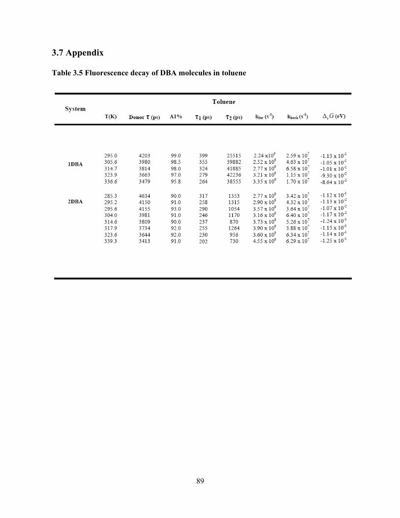
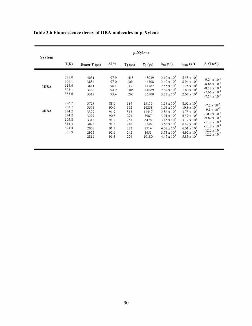
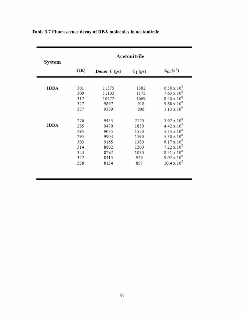
3.3 Results
3.3.1 Emission Spectroscopy:
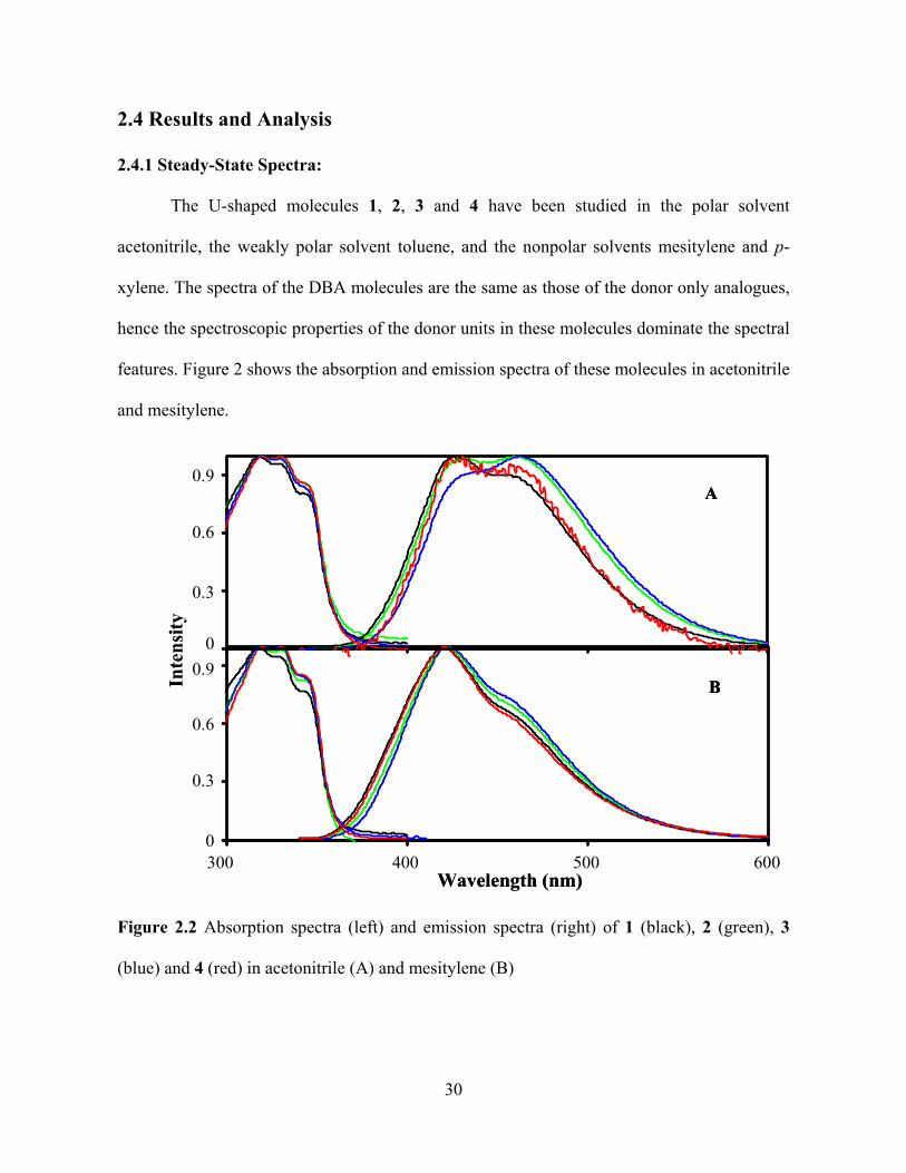
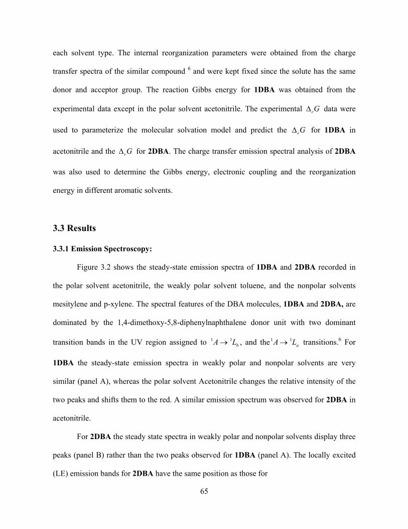
Figure 3.2 shows the steady-state emission spectra of 1DBA and 2DBA recorded in
the polar solvent acetonitrile, the weakly polar solvent toluene, and the nonpolar solvents
mesitylene and p-xylene. The spectral features of the DBA molecules, 1DBA and 2DBA, are
dominated by the 1,4-dimethoxy-5,8-diphenylnaphthalene donor unit with two dominant
transition bands in the UV region assigned to 1 , and the1 transitions.6 For
1DBA the steady-state emission spectra in weakly polar and nonpolar solvents are very
similar (panel A), whereas the polar solvent Acetonitrile changes the relative intensity of the
two peaks and shifts them to the red. A similar emission spectrum was observed for 2DBA in
acetonitrile.
1bA L 1
aA L
For 2DBA the steady state spectra in weakly polar and nonpolar solvents display three
peaks (panel B) rather than the two peaks observed for 1DBA (panel A). The locally excited
(LE) emission bands for 2DBA have the same position as those for
65
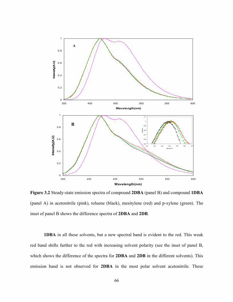
Figure 3.2 Steady-state emission spectra of compound 2DBA (panel B) and compound 1DBA
(panel A) in acetonitrile (pink), toluene (black), mesitylene (red) and p-xylene (green). The
inset of panel B shows the difference spectra of 2DBA and 2DB.
1DBA in all these solvents, but a new spectral band is evident to the red. This weak
red band shifts further to the red with increasing solvent polarity (see the inset of panel B,
which shows the difference of the spectra for 2DBA and 2DB in the different solvents). This
emission band is not observed for 2DBA in the most polar solvent acetonitrile. These
0
0.2
0.8
1
350 400 450 500 550 600
Wavelength(nm)
A
0.4
0.6
Inte
nsi
ty(A
.U)
0
0.2
0.4
0.6
0.8
1
350 400 450 500 550 600
Wavelength(nm)
Inte
nsi
ty(A
.U)
0.5
0.6
0.7
0.8
0.9
1
1.1
2.1 2.2 2.3 2.4 2.5 2.6 2.7
Energy (eV)
Inte
nsit
y
B
66
properties indicate that this emission is a charge-transfer ( ) emission band.12,13
Difference spectra of 2DBA and 2DB in different solvents are shown in the inset of figure 3.2
(also see Fig. 3.3) and were used to calculate values of
0CS S
max . The solvent parameters and the
resulting max values are listed in Table 3.1.
We have analyzed the solvent dependence of the CT fluorescence maximum of
compound 2DBA in terms of the well-known Lippert-Mataga relation (equation 3).14,15 The
frequency of the CT emission band’s maximum intensity is given by
2
0max max3
2f
hca
3
where f = 2 2( 1) /(2 1) ( 1) /(4 2)n n , max is in cm-1; 0
max is the emission
maximum for , a is the effective radius of a spherical cavity that the donor-acceptor
molecule occupies in the solvent,
0f
0CS S
is the difference in dipole moments of the
charge separated state and the ground state, is the Planck constant, c is the velocity of light
in vacuum,
h
is the solvent dielectric constant; and n is the refractive index of the solvent.
This result also incorporates the polarizability of the solute, which was taken equal to 31
3a .
The solvent parameter, f , depends on the static dielectric constant ( S ) and refractive index
(n) of the solvent, and it increases with increasing solvent polarity (see Table 3.1 and also
Fig.3.3). The f parameter quantifies the solvent’s ability to produce a macroscopic
polarization in response to the newly formed charge distribution of the charge separated state.
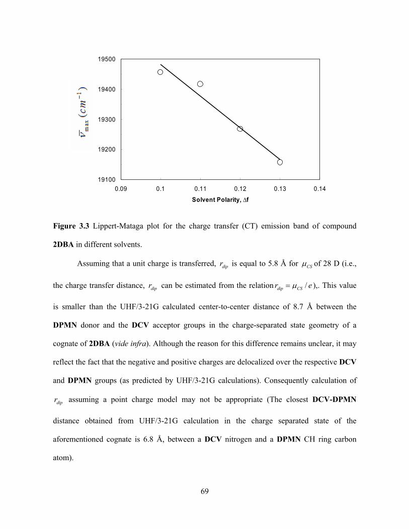
Figure 3.3 shows a Lippert-Mataga plot for 2DBA in the four solvents, where
67
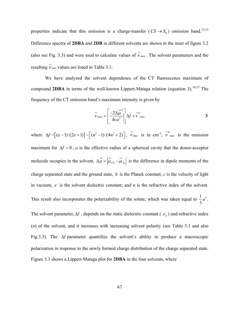
Table 3.1 Charge Transfer (CT) Emission Maxima ( max ) of 2DBA in different solvents
at 295 K and Solvent Parameters, n, S (295K) and f for each solvent
max of the charge transfer band decreases as a function of increasing polarity, or f . A
reasonable linear fit to the data provides a slope of -10500 cm-1. To estimate
from this
slope and Equation 3, a cavity radius, a, of 7.66 Å was used. This value was chosen because
previous work found it as a best fit to the rG data of 1DBA to the molecular solvation
model. Solving equation 3 for
gives a value of 22 D for the difference between the
charge-separated state and the ground state dipole moments. Using 5.75 D for the ground state
dipole moment5 and assuming that the dipoles are collinear, the dipole moment of the charge
separated state is ~28 D, which is close to the dipole moment of the charge separated state
used in the molecular solvation model analysis. This value is also in good agreement with the
HF/3-21G calculated value of 28.6 D for a simulacrum of the charge separated state of 1DBA
(the dipole moments of the charge-separated states of 1DBA and 2DBA should be similar).
68
19100
19200
19300
19400
19500
0.09 0.1 0.11 0.12 0.13 0.14
Solvent Polarity, ∆f
Figure 3.3 Lippert-Mataga plot for the charge transfer (CT) emission band of compound
2DBA in different solvents.
Assuming that a unit charge is transferred, is equal to 5.8 Å for dipr CS of 28 D (i.e.,
the charge transfer distance, can be estimated from the relationdipr /Sdip Cr e ),. This value
is smaller than the UHF/3-21G calculated center-to-center distance of 8.7 Å between the
DPMN donor and the DCV acceptor groups in the charge-separated state geometry of a
cognate of 2DBA (vide infra). Although the reason for this difference remains unclear, it may
reflect the fact that the negative and positive charges are delocalized over the respective DCV
and DPMN groups (as predicted by UHF/3-21G calculations). Consequently calculation of
assuming a point charge model may not be appropriate (The closest DCV-DPMN
distance obtained from UHF/3-21G calculation in the charge separated state of the
aforementioned cognate is 6.8 Å, between a DCV nitrogen and a DPMN CH ring carbon
atom).
dipr
69
3.3.2 Analysis of Charge-Transfer Emission Spectra of 2DBA to obtain and r G 0
The charge recombination driving force for 2DBA was estimated by simulation of the
charge transfer emission lineshape predicted by Marcus16 ; i.e.
2
0
0
(( ) .exp
! 4
S jrec CS
emission CSj
jh G he SI
j kT
)
4
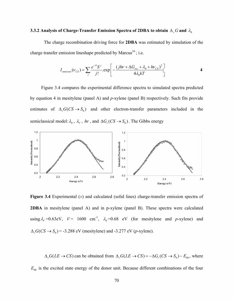
Figure 3.4 compares the experimental difference spectra to simulated spectra predicted
by equation 4 in mesitylene (panel A) and p-xylene (panel B) respectively. Such fits provide
estimates of and other electron-transfer parameters included in the
semiclassical model:
0(rG CS S
0
)
, V , h , and 0(rG CS S ) . The Gibbs energy
0.2
0.4
0.6
0.8
1
1.2
2 2.2 2.4 2.6 2.8
Energy (eV)
Inte
nsit
y(N
orm
alis
ed)
0.2
0.4
0.6
0.8
1
1.2
2 2.2 2.4 2.6
Energy (eV)
Inte
nsit
y(N
orm
alis
ed)
2.8
Figure 3.4 Experimental (o) and calculated (solid lines) charge-transfer emission spectra of
2DBA in mesitylene (panel A) and in p-xylene (panel B). These spectra were calculated
using V =0.63eV, = 1600 cm-1, 0 =0.68 eV (for mesitylene and p-xylene) and
= -3.288 eV (mesitylene) and -3.277 eV (p-xylene). 0(r S )
) 0
G CS
(rG LE CS can be obtained from 0 0( ) ( )r rG LE CS G CS S E , where
is the excited state energy of the donor unit. Because different combinations of the four 00E
70
parameters can accurately reproduce the experimental line shapes, the fitting parameters were
constrained in the following way. The fits in fig. 3.4 were done with a constant value 0.63 eV
for the V parameter and a value of ~1600 cm-1; these values were used previously for
similar molecules and were chosen for consistency with earlier work. Only 0 and
were adjusted in different solvents to optimize the fit. 0rG C S ( S )
2
0 ( )eV
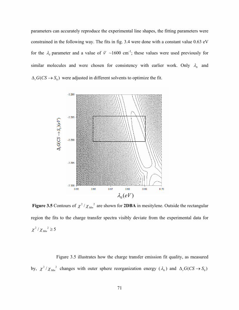
Figure 3.5 Contours of 2 / Min are shown for 2DBA in mesitylene. Outside the rectangular
region the fits to the charge transfer spectra visibly deviate from the experimental data for
2 2/ 5Mi
2
n
2 /
Figure 3.5 illustrates how the charge transfer emission fit quality, as measured
by, Min changes with outer sphere reorganization energy ( 0 ) and 0( )rG C SS
71
values used in the fitting. The Min represents the smallest value of obtained from the
fitting. The boxed region in this case identifies the range for 0 and over
which the difference between the experimental and theoretical charge transfer emission
spectra deviate visibly with a change of the . Table 3.2 lists the different values
of and
0( )rG CS S
2 2/ Min 5
0( )rG CS S 0 obtained from the CT spectral fitting for different solvents. The
line-shape derived estimates of 0 increases with increasing solvent dielectric constant.
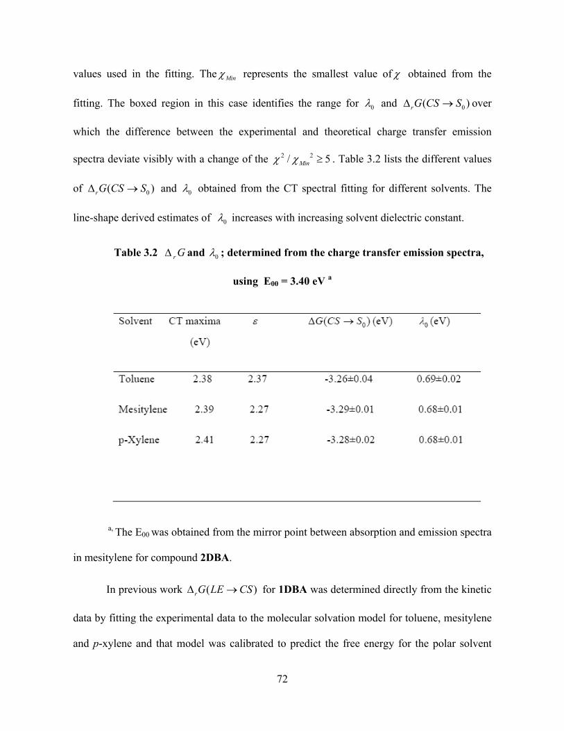
Table 3.2 and r G 0 ; determined from the charge transfer emission spectra,
using E00 = 3.40 eV a
a, The E00 was obtained from the mirror point between absorption and emission spectra
in mesitylene for compound 2DBA.
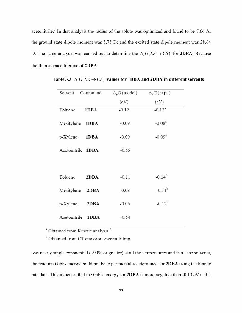
In previous work for 1DBA was determined directly from the kinetic
data by fitting the experimental data to the molecular solvation model for toluene, mesitylene
and p-xylene and that model was calibrated to predict the free energy for the polar solvent
( )G L CS r E
72
acetonitrile.6 In that analysis the radius of the solute was optimized and found to be 7.66 Å;
the ground state dipole moment was 5.75 D; and the excited state dipole moment was 28.64
D. The same analysis was carried out to determine the ( )rG LE CS for 2DBA. Because
the fluorescence lifetime of 2DBA
Table 3.3 values for 1DBA and 2DBA in different solvents (rG LE CS )
was nearly single exponential (~99% or greater) at all the temperatures and in all the solvents,
the reaction Gibbs energy could not be experimentally determined for 2DBA using the kinetic
rate data. This indicates that the Gibbs energy for 2DBA is more negative than -0.13 eV and it
73
can not be determined directly form the experiment. This observation implies that for
2DBA is more negative than that for 1DBA. The charge transfer fit parameters of 2DBA in
different solvents were used to determine the
r G
( )rG LE CS for 2DBA. Table 3.3 compares
the of 1 DBA and 2DBA. The Gibbs energy becomes more negative as the solvent
becomes more polar, progressing from mesitylene and p-xylene, which have the least
negative , to toluene which is more negative, and finally to acetonitrile which
is the most negative. Table 3.3 also reveals a reasonable agreement between the Gibbs energy
for 2DBA obtained from the charge transfer emission spectral fitting and that predicted from
the molecular solvation model.
r G
( )rG LE CS
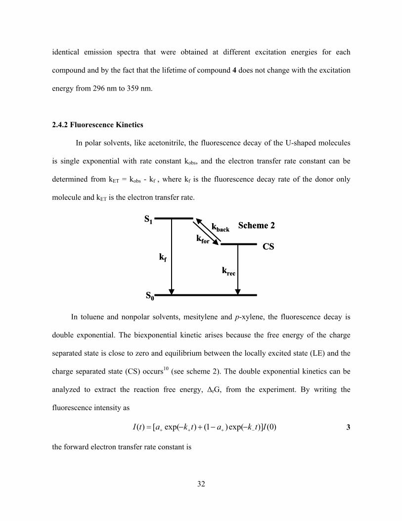
3.3.3 Kinetic analysis
With the reaction free energy and the internal reorganization energy parameters from
the previous studies, it is possible to fit the temperature dependent rate constant data and
extract the electronic coupling │VCS│ and the solvent reorganization energy λ0 for the charge
separation process. │VCS│ is treated as a temperature independent quantity, whereas the
solvent reorganization energy has a temperature dependence because the solvation is
temperature dependent. The temperature dependence of the solvent reorganization energy was
predicted from the molecular solvation model and the best fit was used to extract the solvent
reorganization energy at 295 K, as described previously. The fit of the temperature dependent
rate constant data was used to determine the electronic coupling │VCS│ and λ0 (295 K), listed
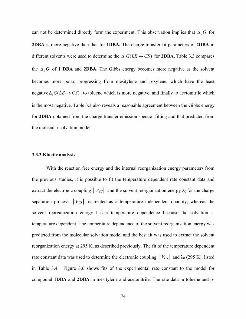
in Table 3.4. Figure 3.6 shows fits of the experimental rate constant to the model for
compound 1DBA and 2DBA in mesitylene and acetonitrile. The rate data in toluene and p-
74
xylene behave similarly. The reverse order of the electron transfer rate for 1DBA and 2DBA
in mesitylene and acetonitrile can be explained by their different reorganization energy
value.1
Figure 3.6 Experimental rate constant data are plotted versus 1/T, for 1DBA in mesitylene
(▲) and acetonitrile (●), and for 2DBA in mesitylene (∆) and in acetonitrile (o). The line
represe
puted using the
charge transfer emission spectra (Table 3.4), as described in the next section
nts the best fits to semiclassical equation.
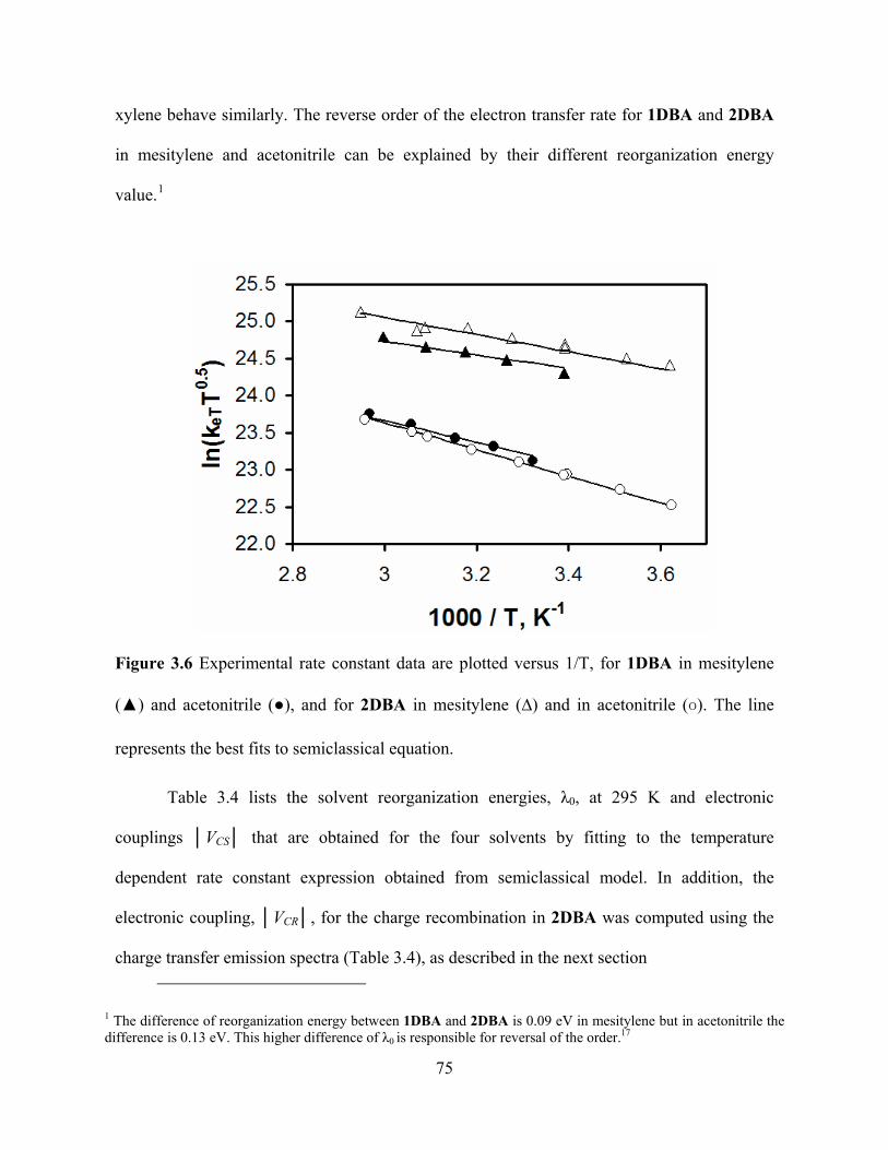
Table 3.4 lists the solvent reorganization energies, λ0, at 295 K and electronic
couplings │VCS│ that are obtained for the four solvents by fitting to the temperature
dependent rate constant expression obtained from semiclassical model. In addition, the
electronic coupling, │VCR│, for the charge recombination in 2DBA was com
1 The difference of reorganization energy between 1DBA and 2DBA is 0.09 eV in mesitylene but in acetonitrile the difference is 0.13 eV. This higher difference of λ0 is responsible for reversal of the order.17
75
Ta from the
kinetic fit and from CT emission spectra) for 1DBA and 2DBA.
ble 3.4 Best fit of electronic coupling and reorganization energy (
ng obtained form the CT emission spectral analysis using the distance
d Reorganization energy obtained from the CT emission spectra fit.
a Coupling obtained from the best fit rate data
b Coupli
5.8 Å
c Reorganization energy obtained from best fit rate data
76
.
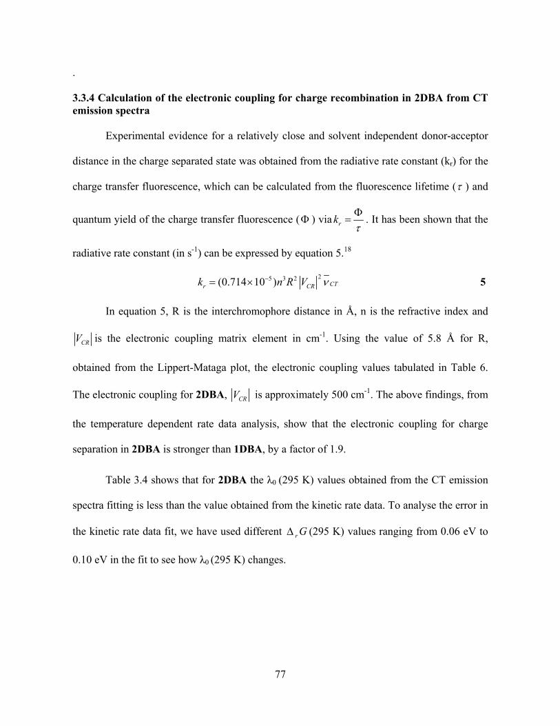
3.3.4 Calculation of the electronic coupling for charge recombination in 2DBA from CT emissio
d the flu
n spectra
Experimental evidence for a relatively close and solvent independent donor-acceptor
distance in the charge separated state was obtained from the radiative rate constant (kr) for the
charge transfer fluorescence, which can be calculate from orescence lifetime ( ) and
quantum yield of the charge transfer fluorescence ( ) via rk
. It has been shown that the
radiativ can be expressed by equation 5e rate constant (in s-1) .18
2 5 3 2(0.714 10 ) CTr CRk n R V 5
In equation 5, R is the interchromophore distance in Å, n is the refractive index and
CRV is the electronic coupling matrix element in cm-1. Using the value of 5.8 Å for R,
obtained from the Lippert-Mataga plot, the electronic coupling values tabulated in Table 6.
The electronic coupling for 2DBA, CRV is approximately 500 cm-1. The above findings, from
the temperature dependent rate data analysis, show that the electronic coupling for charge
separat
the
ion in 2DBA is stronger than 1DBA, by a factor of 1.9.
Table 3.4 shows that for 2DBA the λ0 (295 K) values obtained from the CT emission
spectra fitting is less than the value obtained from kinetic rate data. To analyse the error in
the kinetic rate data fit, we have used different r G (295 K) values ranging from 0.06 eV to
0.10 eV in the fit to see how λ0 (295 K) changes.
77
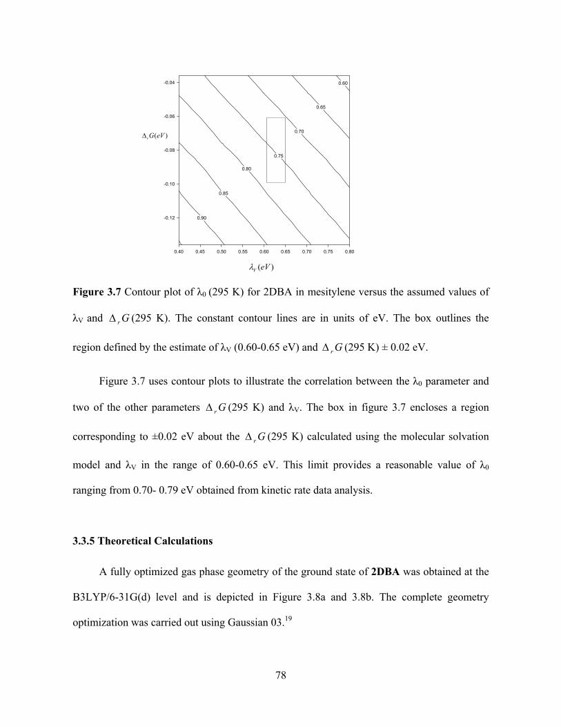
.7 C
outlines the
Figure 3 ontour plot of λ0 (295 K) for 2DBA in mesitylene versus the assumed values of
λV and r G (295 K). The constant contour lines are in units of eV. The box
region defined by the estim
0.60
0.65
0.70
0.75
0.80
0.85
0.90
0.40 0.45 0.50 0.55 0.60 0.65 0.70 0.75 0.80
-0.12
-0.10
-0.08
-0.06
-0.04
( )rG eV
( )V eV
ate of λV (0.60-0.65 eV) and r G (295 K) ± 0.02 eV.
Figure 3.7 uses contour plots to illustrate the correlation between the λ0 parameter and
two of the other parameters r G (295 K) and λV. The box in figure 3.7 encloses a region
corresponding to ±0.02 eV about the r G (295 K) calculated using the molecular solvation
model and λV in the range of 0.60-0.65 eV. This limit provides a reasonable value of λ0
ranging from 0.70- 0.79 eV obtained from kinetic rate data analysis.
e 3.8a and 3.8b. The complete geometry
optimization was carried out using Gaussian 03.19
3.3.5 Theoretical Calculations
A fully optimized gas phase geometry of the ground state of 2DBA was obtained at the
B3LYP/6-31G(d) level and is depicted in Figur
78
o
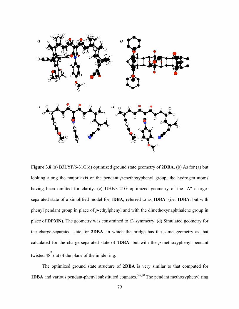
Figure 3.8 (a) B3LYP/6-31G(d) optimized ground state geometry of 2DBA. (b) As for (a) but
looking along the major axis of the pendant p-methoxyphenyl group; the hydrogen atoms
having been omitted for clarity. (c) UHF/3-21G optimized geometry of the 1A'' charge-
separated state of a simplified model for 1DBA, referred to as 1DBA' (i.e. 1DBA, but with
phenyl pendant group in place of p-ethylphenyl and with the dimethoxynaphthalene group in
place of DPMN). The geometry was constrained to CS symmetry. (d) Simulated geometry for
the charge-separated state for 2DBA, in which the bridge has the same geometry as that
calculated for the charge-separated state of 1DBA' but with the p-methoxyphenyl pendant
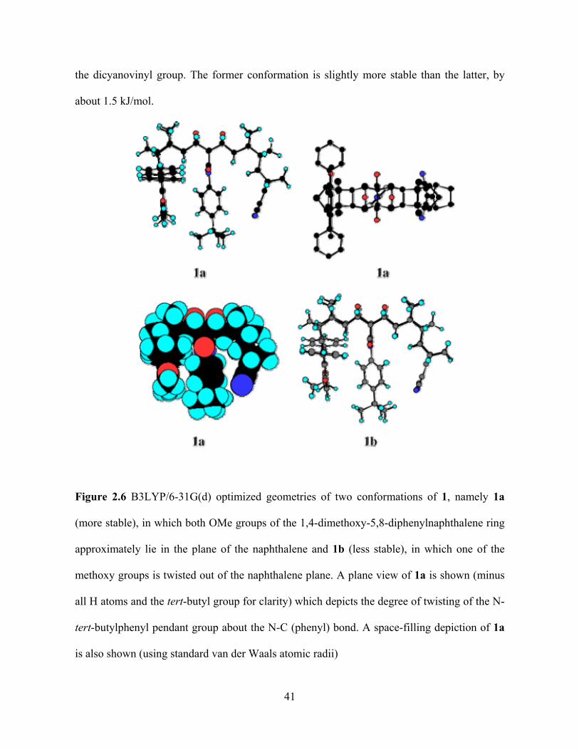
twisted 48 out of the plane of the imide ring.
The optimized ground state structure of 2DBA is very similar to that computed for
1DBA and various pendant-phenyl substituted cognates.5,6,20 The pendant methoxyphenyl ring
79
is twisted 48o
with respect to the plane of the imide ring, the closest distance between the
DPMN and DCV chromophore units is 9.2 Å which is between a CH carbon atom of the
former and an N atom of the latter, and the closest distances between the pendant group and
the DPMN and DCV chromophore units are 3.8 - 3.9 Å (c.f. 47o
, 9.4 Å and 3.8 - 3.9 Å,
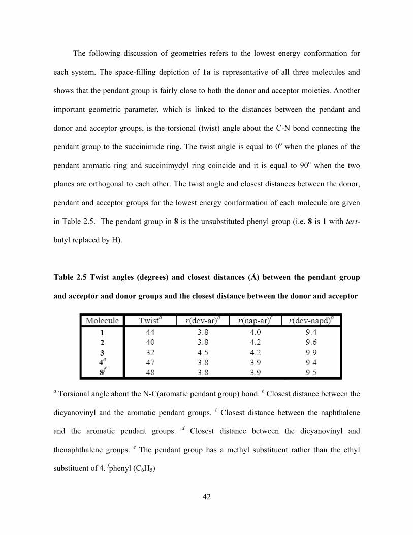
respectively for the compound having methylphenyl as pendant group).
Because of the large sizes of these U-shaped molecules, it was not feasible to compute
the optimized geometry of the locally excited state of 2DBA, which is relevant to the
mechanism of photoinduced charge separation, using the CIS method. The strong similarities
found between the ground state geometries of 1DBA and 2DBA most likely holds for the
locally excited states of these systems. Consequently, the greater magnitude of the electronic
coupling for photoinduced charge separation in 2DBA, compared to 1DBA, is unlikely to be
caused by structural differences in the two systems. Two important classes of virtual ionic
states namely +DPMN-pendant- and +pendant-DCV- contribute to the coupling for
photoinduced electron transfer in these systems. However, for charge transfer from the locally
excited state of the donor to the acceptor, the former ionic state is expected to be more
important. Comparison with experimental data on monosubstituted benzenes suggests that the
pendant groups’ electron affinities (EA) (anisole EA= -1.09 eV and ethyl benzene EA= -1.17
eV21) are similar, but that 2DBA should have a larger electronic coupling than 1DBA. It may
be that the second virtual ionic state +pendant-DCV- contributes, when the pendant group has
a low ionization potential (IP) value. The IP for toluene and anisole are 8.83 and 8.39 eV
respectively.22 Whether one coupling mechanism dominates over the other, could, in
principle, be resolved by studying a U-shaped system in which an electron withdrawing group
is attached to the pendant aromatic ring at position 3 or 4. Unfortunately, all attempts to
80
synthesize such a system have so far met with failure.
Earlier UHF/3-21G gas phase calculations of charge-separated states revealed
remarkable electrostatically driven changes in their geometries, compared to their ground
state structures.5,18,23 Regarding the U-shaped systems discussed in this paper, we were
successful only in optimizing, at the UHF/3-21G level, the geometry of the charge-separated
state of a cognate of 1DBA, termed as 1DBA', in which the pendant group was phenyl and the
dimethoxynaphthalene group, DMN, was the donor moiety (in place of DPMN).
Furthermore, the geometry of the charge-separated state of 1DBA' was constrained to possess
CS symmetry;24
within this constraint, the electronic state of this charge-separated state is 1A'',
thereby preventing collapse of the wavefunction to the 1A' ground state during the geometry
optimization.23,24 The resulting optimized gas phase structure for the charge-separated state of
1DBA' is shown in Fig. 3.8c, a particularly noteworthy feature being the strong
pyramidalization of the DCV anion radical towards the DPMN cation radical whose rings are
slightly bent, in the direction of the DCV moiety. Due to the imposed CS symmetry constraint,
the phenyl pendant group is roughly parallel to the imide ring. Such a conformation, in which
the phenyl ring eclipses the imide carbonyl groups should be unstable, as it is in the ground
state, and the relaxed phenyl-imide conformation in the charge separated state of 1DBA'
should resemble that computed for the ground state structure, i.e. with the phenyl ring twisted
480 with respect to the imide plane as depicted by the simulated structure in Fig. 3.8d.
The calculated UHF/3-21G dipole moment of 1DBA' is 28.6 D5 which is in good
accord with the value of 28 D for 2DBA, determined from the Lippert-Mataga plot. Also the
distance between the centroids of the DPMN and DCV chromophore units in 1DBA' was
calculated to be 8.7 Å, although the closest contact between non-hydrogen atoms of the donor
81
and acceptor groups is only 6.8 Å. The closest non-hydrogen atom contacts between the
pendant group in the charge-separated state of 1DBA' and the DMN and DCV chromophores
are 3.6 and 3.2 Å respectively and these are even smaller in the more reasonable structure
depicted in Fig. 3.8d: 2.65 and 2.7 Å respectively. The significantly smaller chromophore-
pendant contacts of 2.7 Å in the simulated charge-separated state (Fig.8d), compared to 3.8 Å
in the ground state of 1DBA (Fig. 3.8a) could well be responsible for the observed stronger
electronic coupling of 453-512 cm-1 for charge recombination compare to charge separation,
which is 274 cm-1 in 2DBA.
3.4 Discussion
The electron transfer rate constant from the locally excited state of DPMN to DCV for
2DBA is larger than that for 1DBA in toluene, mesitylene and p-xylene solvents. This
increase arises from the greater magnitude of the electronic coupling in 2DBA, as found from
analysis of the temperature dependent rate data. It is important to note that the electronic
coupling obtained from the CT emission is the coupling between the charge separated state
and the ground state (the charge recombination pathway) whereas the kinetic rate data provide
the coupling between the locally excited state and the charge separated state. Whereas 1DBA
does not display charge transfer fluorescence, 2DBA does, presumably because the magnitude
of CRV for 2DBA is substantially larger than for 1DBA. Although the CT emission for 2DBA
is also not observed in acetonitrile, it is likely due to the non-radiative charge recombination
82
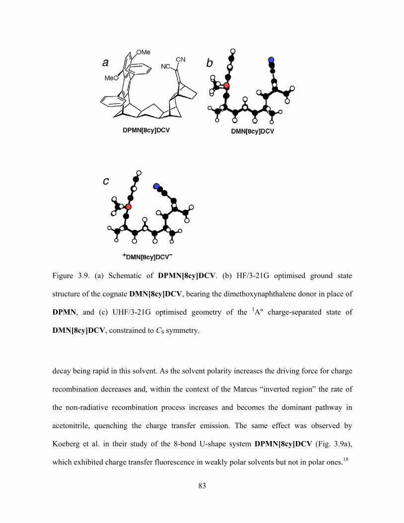
Figure 3.9. (a) Schematic of DPMN[8cy]DCV. (b) HF/3-21G optimised ground state
structure of the cognate DMN[8cy]DCV, bearing the dimethoxynaphthalene donor in place of
DPMN, and (c) UHF/3-21G optimised geometry of the 1A'' charge-separated state of
DMN[8cy]DCV, constrained to CS symmetry.
decay being rapid in this solvent. As the solvent polarity increases the driving force for charge
recombination decreases and, within the context of the Marcus “inverted region” the rate of
the non-radiative recombination process increases and becomes the dominant pathway in
acetonitrile, quenching the charge transfer emission. The same effect was observed by
Koeberg et al. in their study of the 8-bond U-shape system DPMN[8cy]DCV (Fig. 3.9a),
which exhibited charge transfer fluorescence in weakly polar solvents but not in polar ones.18
83
It is illuminating to compare the strength of the electronic coupling for CT fluorescence
of ~500 cm-1 for 2DBA with the value of 374 cm-1 (in benzene) for DPMN[8cy]DCV.18 Both
systems possess similar U-shape configurations, but the latter lacks a pendant group. Even
though the DPMN and DCV chromophores are connected by twelve bonds in 2DBA,
compared to only eight bonds in DPMN[8cy]DCV (see Fig. 3.9a), the electronic coupling
strength for CT fluorescence in the former molecule is larger than that for the latter. This
observation is best understood if the charge recombination (and charge separation) in 2DBA
takes place by the through-pendant mechanism, rather than by a through-bridge (i.e. through-
bond) mechanism. The charge recombination mechanism in DPMN[8cy]DCV is discussed
below.
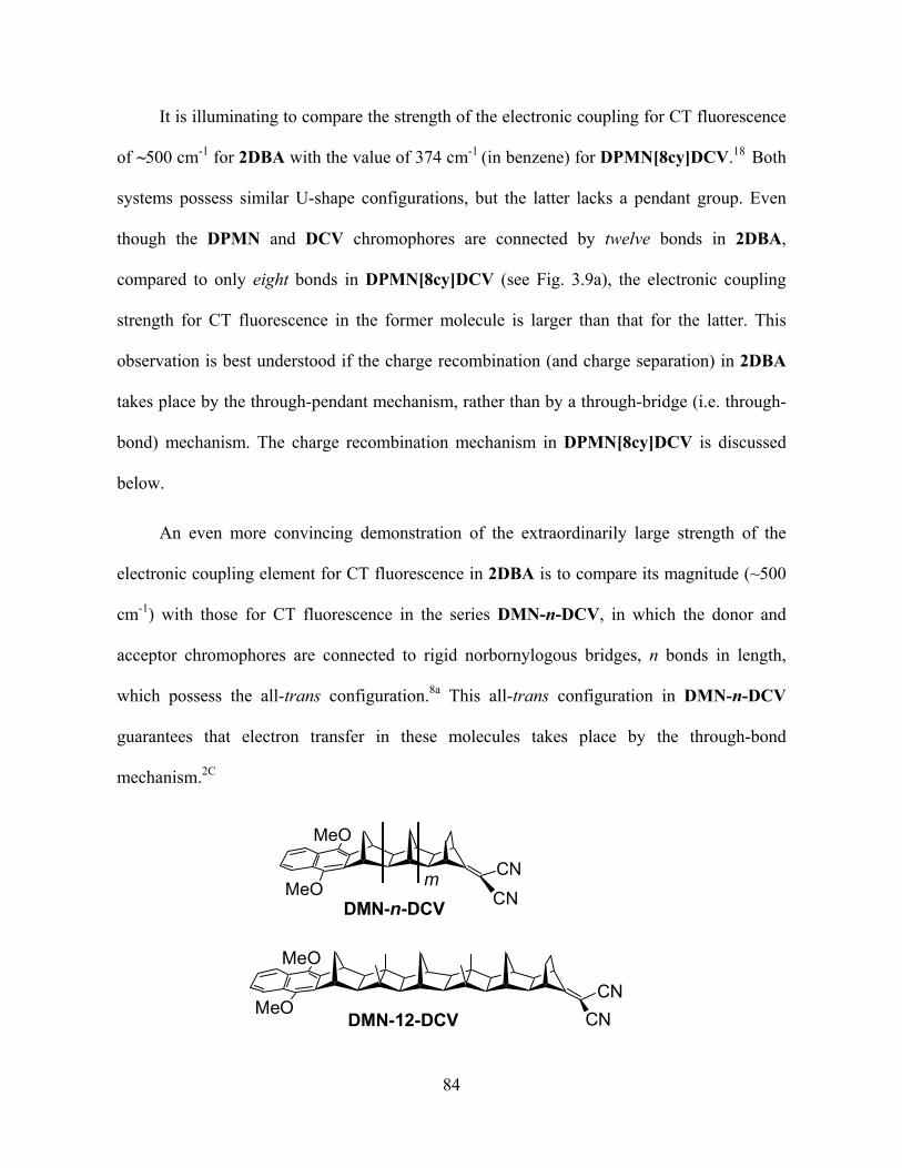
An even more convincing demonstration of the extraordinarily large strength of the
electronic coupling element for CT fluorescence in 2DBA is to compare its magnitude (~500
cm-1) with those for CT fluorescence in the series DMN-n-DCV, in which the donor and
acceptor chromophores are connected to rigid norbornylogous bridges, n bonds in length,
which possess the all-trans configuration.8a This all-trans configuration in DMN-n-DCV
guarantees that electron transfer in these molecules takes place by the through-bond
mechanism.2C
MeO
MeOCN
CNDMN-12-DCV
CN
CN
MeO
MeO m
DMN-n-DCV
84
Extrapolating the experimental CRV values for the 4-, 6-, 8- and 10-bond systems leads to a
predicted CRV value of ~6 cm-1 for the 12-bond system DMN-12-DCV. Because the 12-bond
norbornylogous bridge in 2DBA possesses two cisoid kinks, through-bridge-mediated
electronic coupling in this molecule should be significantly weaker than that through the all-
trans bridge in DMN-12-DCV.2b,2c In fact CRV for 2DBA is ~90 times stronger than that
estimated for DMN-12-DCV. Clearly, charge recombination from the charge- separated state
of 2DBA is not taking place by a through-bridge-mediated mechanism. These findings,
together with the observation that the strength of the electronic coupling for photoinduced
charge separation for 2DBA is greater than that for 1DBA leads to the unequivocal conclusion
that charge separation and charge recombination processes must be taking place via the
pendant aromatic ring in both 2DBA and 1DBA.
There is strong evidence that charge recombination in DPMN[8cy]DCV takes place
directly, through-space, between the two chromophores, which is facilitated by the
electrostatically enforced proximity of the two chromophores in the charge-separated state of
this species (see Fig. 3.9c). Thus, the distance between the two centroids in the charge-
separated state of DPMN[8cy]DCV, based on a model system (Fig. 3.9c), is only 4.4 Å,18
which is sufficiently small to promote strong through-space interchromophore coupling in this
species.25
The distances between the pendant group and DPMN and DCV chromophores in
the charge-separated state of 1DBA' are between 3.4 Å and 2.7 Å, depending on the twist
angle of the pendant phenyl ring (see previous section). These distances are significantly
smaller than the aforementioned value computed for the charge-separated state of
DPMN[8cy]DCV. Thus, the finding that the strength of the electronic coupling for CT
85
fluorescence is substantially larger for 2DBA, compared to that for DPMN[8cy]DCV, is
understandable.
A fit of the rate constant data as a function of temperature to Equation 2 was used to
extract values for the solvent reorganization energy (see Table 3.4) for 1DBA and 2DBA. The
solvent reorganization energy values of 2DBA are higher than 1DBA in all the solvents. The
difference between their solvent reorganization energy values is highest for the most polar
solvent acetonitrile and least for p-xylene. Since the pendant groups in 1DBA and 2DBA have
comparable sizes, the difference is likely caused by differences in the polarities of the pendant
groups in these molecules, the electronegative oxygen atom making the methoxyphenyl
pendant group in 2DBA more polar than ethylphenyl group in 1DBA. The CT emission fit
was also used to determine the solvent reorganization energy for charge recombination in
2DBA (Table 3.4). The values obtained from CT emission spectra fitting is somewhat smaller
than the values obtained from the kinetic rate data and correlates with more negative values of
obtained from CT emission fit (Table 3.3). rG
The values for 1DBA were obtained from the kinetic fit of the experimental data
to the molecular solvation model whereas fitting to the CT emission was used to calculate
values of 2DBA experimentally in different solvents. The magnitude of is least
negative in p-xylene and is most negative in polar solvent acetonitrile. The for 2DBA
can not be determined from kinetic fit as
rG
rG rG
Gr
rG is too negative (from CT emission fitting);
however the estimated free energy obtained from the molecular solvation model for 2DBA is
somewhat lower than the free energy of 1DBA. This finding indicates that there is some error
associated with the fitting. To estimate the error we have used the contour plot of
86
reorganization energy values as a function of different free energy values in the fit in
mesitylene (Fig. 3.7). The plot provides reasonable values for the reorganization energy
ranging from 0.70-0.79 eV and values close to the values obtained from the CT emission
fit.
rG
3. 5 Conclusion
The electron transfer in U-shaped molecules 1DBA and 2DBA containing two different
pendant groups in the cleft between the donor and acceptor group was studied. 2DBA shows
CT emission in nonpolar and weakly polar solvents. The magnitude of the electronic coupling
for photoinduced charge separation in 1DBA and 2DBA were found to be 147 and 274 cm-1,
respectively. The origin of this difference lies in the electronic nature of the pendant aromatic
group, since charge separation occurs by tunneling through the pendant group, rather than
through the bridge. The charge transfer fluorescence for 2DBA in non-polar solvents was
used to determine the electronic coupling for charge recombination, CRV , the magnitude of
which is ~ 500 cm-1, much larger than that for charge separation. This difference can be
explained by changes in the geometry of the molecule in the relevant states; because of
electrostatic effects, the DPMN and DCV chromophores are about 1Å closer to the pendant
group in the CS state than in the locally excited state. Consequently the through-pendant-
group electronic coupling is stronger in the CS state – which controls the CT fluorescence
process – than in the locally excited state – which controls the CS process. The magnitude of
CRV for 2DBA is almost two orders of magnitude greater than that in DMN-12-DCV, having
the same length bridge as for the former molecule, but lacking a pendant group. This result
unequivocally demonstrates the operation of the through-pendant-group mechanism of
electron transfer in the pendant-containing U-shaped systems of the type 1DBA and 2DBA.
87
Our observation of the modulation of the strength of electronic coupling in the U-shaped
system 2DBA, brought about by electrostatically driven changes in molecular geometry,
suggests an intriguing approach to the generation of long-lived charge-separated species:
build a U-shaped system possessing a doubly positively chaged acceptor, D-B-A2+ (e.g. A2+ =
viologen). Photoinduced electron transfer should generate D+-B-A+. Repulsive electrostatic
interactions should drive the singly positively chaged chromophores further apart, thereby
weakening the electronic coupling for charge recombination. Such an effect has been
observed and explained in terms of this mechanism.26
3. 6 Acknowledgement
We acknowledge financial support from the Australian Research Council and the US
National Science Foundation (CHE-041545).
88
3.7 Appendix
Table 3.5 Fluorescence decay of DBA molecules in toluene
89
Table 3.6 Fluorescence decay of DBA molecules in p-Xylene
90
Table 3.7 Fluorescence decay of DBA molecules in acetonitrile
91
3. 8 References
1. (a) Barbara, P. F.; Meyer, T. J.; Ratner, M. A. J. Phys. Chem. 1996, 100, 13148. (b)
Electron Transfer-From Isolated Molecules to Biomolecules, Adv. Chem. Phys. Jortner, J.;
Bixon, M., Eds.; Wiley: New York, 1999.
2. (a) Hush, N. S.; Paddon-Row, M. N.; Cotsaris, E.; Oevering, H.; Verhoeven, J. W.;
Heppener, M. Chem. Phys. Lett. 1985, 117, 8. (b) Oliver, A. M.; Craig, D. C.; Paddon-
Row, M. N.; Kroon, J.; Verhoeven, J. W. Chem. Phys. Lett. 1988, 150, 366. (c) Paddon-
Row, M. N. Acc. Chem. Res. 1994, 27, 18.
3. (a) Zeng, Y.; Zimmt, M. B. J. Phys. Chem. 1992, 96, 8395. (b) Oliver, A. M.; Paddon-
Row, M. N.; Kroon, J.; Verhoeven, J. W. Chem. Phys. Lett. 1992, 191, 371.
4. (a) Closs, G. L.; Miller, J. R. Science 1988, 240, 440. (b) Guldi, D. M.; Luo, C.; Prato, M.;
Troisi, A.; Zerbetto, F.; Scheloske, M.; Dietel, E.; Bauer, W.; Hirsch, A.; J. Am. Chem.
Soc. 2001, 123, 9166.
5. Napper, A. M.; Head, N. J.; Oliver, A. M.; Shephard, M. J.; Paddon-Row, M. N.; Read, I.;
Waldeck, D. H. J. Am. Chem. Soc. 2002, 124, 10171.
6. Liu, M.; Chakrabarti, S.; Waldeck, D. H.; Oliver, A. M.; Paddon-Row, M. N. Chem. Phys.
2006, 324, 72.
7. Napper, A. M.; Read, I.; Waldeck, D. H.; Head, N.J.; Oliver, A. M.; Paddon-Row, M. N.
J. Am. Chem. Soc. 2000, 122, 5220.
92
8. (a) Oevering, H.; Verhoeven, J. W.; Paddon-Row, M. N.; Warman, J. M.
Tetrahedron 1989, 45, 4751. (b) Oevering, M. N.; Paddon-Row, M. N.; Heppener,
H.; Oliver, A. M.; Cotsaris, E.; Verhoeven, J. H.; Hush, N. S. J. Am. Chem. Soc.
1987, 109, 3258.
9. Kumar, K.; Kurnikov, I. V.; Beratan, D. N.; Waldeck, D. H.; Zimmt, M. B.
J. Phys. Chem. A, 1998, 102, 5529.
10. Read, I.; Napper, A. M.; Zimmt, M. B.; Waldeck, D. H. J. Phys. Chem. A 2000,
104, 9385.
11. Matyushov, D. V.; Voth, G. A. J. Chem. Phys. 1999, 111, 3630.
12. (a) Paddon-Row, M. N.; Oliver, A. M.; Warman, J. M.; Smit, K. J.; de Hass, M.
P.; Oevering, H.; Verhoeven, J. W. J. Phys. Chem. 1988, 92, 6958. (b) Warman, J.
M.; Smit, K. J.; de Hass, M. P.; Jonker, S. A.; Paddon-Row, M. N.; Oliver, A. M.;
Kroon, J.; Oevering, H.; Verhoeven, J. W. J. Phys. Chem. 1991, 95, 1979.
13. Wasielewski, M. R.; Minsek, D. W.; Niemczyk, M. P.; Svec, W. A.; Yang, N. C.
J. Am. Chem. Soc. 1990, 112, 2823.
14. Morais, J.; Huang, R. R.; Grabowski, J. J.; Zimmt, M. B. J. Phys. Chem. 1993, 97, 13138.