Recommendation ITU-R M.1849-1 (09/2015)

Technical and operational aspects of ground-based meteorological radars

M Series

Mobile, radiodetermination, amateur

and related satellite services

ii Rep. ITU-R M.1849-1

Foreword

The role of the Radiocommunication Sector is to ensure the rational, equitable, efficient and economical use of the radio-

frequency spectrum by all radiocommunication services, including satellite services, and carry out studies without limit

of frequency range on the basis of which Recommendations are adopted.

The regulatory and policy functions of the Radiocommunication Sector are performed by World and Regional

Radiocommunication Conferences and Radiocommunication Assemblies supported by Study Groups.

Policy on Intellectual Property Right (IPR)

ITU-R policy on IPR is described in the Common Patent Policy for ITU-T/ITU-R/ISO/IEC referenced in Annex 1 of

Resolution ITU-R 1. Forms to be used for the submission of patent statements and licensing declarations by patent holders

are available from http://www.itu.int/ITU-R/go/patents/en where the Guidelines for Implementation of the Common

Patent Policy for ITU-T/ITU-R/ISO/IEC and the ITU-R patent information database can also be found.

Series of ITU-R Recommendations

(Also available online at http://www.itu.int/publ/R-REC/en)

Series Title

BO Satellite delivery

BR Recording for production, archival and play-out; film for television

BS Broadcasting service (sound)

BT Broadcasting service (television)

F Fixed service

M Mobile, radiodetermination, amateur and related satellite services

P Radiowave propagation

RA Radio astronomy

RS Remote sensing systems

S Fixed-satellite service

SA Space applications and meteorology

SF Frequency sharing and coordination between fixed-satellite and fixed service systems

SM Spectrum management

SNG Satellite news gathering

TF Time signals and frequency standards emissions

V Vocabulary and related subjects

Note: This ITU-R Recommendation was approved in English under the procedure detailed in Resolution ITU-R 1.

Electronic Publication

Geneva, 2015

ITU 2015

All rights reserved. No part of this publication may be reproduced, by any means whatsoever, without written permission of ITU.

Rec. ITU-R M.1849-1 1

RECOMMENDATION ITU-R M.1849-1*

Technical and operational aspects of ground-based meteorological radars

(2009-2015)

Scope

This Recommendation addresses the important technical and operational characteristics of

meteorological radars, describes the related products provided, highlights their major specificities,

discusses the effects of interference on meteorological radars and develops related interference

protection criteria. This text is limited to ground-based weather radars and does not include wind

profiler radars, also used for meteorological purposes, which are covered in a separate

ITU-R Recommendation.

Keywords

Radar, meteorological, protection

Abbreviations/Glossary

CASA Centre for collaborative adaptive sensing of the atmosphere

GC Ground clutter

Pd Probability of detection

PRF Pulse repetition frequency

PRT Pulse repetition time

SAR Synthetic aperture radar

VAD Vertical azimuth display

VCP Volume coverage pattern

WTC Wind turbine clutter

The ITU Radiocommunication Assembly,

considering

a) that antenna, signal propagation, target detection, and large necessary bandwidth

characteristics of radar to achieve their functions are optimum in certain frequency bands;

b) that representative technical and operational characteristics of meteorological radars are

required to determine the feasibility of introducing new types of systems into frequency bands in

which meteorological radars are operated;

c) that procedures and methodologies are needed to analyse compatibility between

meteorological radars and other services to which the frequency band is allocated;

d) that technical and operational characteristics of meteorological radars are specific compared

to other radar types and justify a separate ITU-R Recommendation;

* This Recommendation should be brought to the attention of the World Meteorological Organization

(WMO).

2 Rep. ITU-R M.1849-1

e) that meteorological radars mainly operate in the frequency bands 2 700-2 900 MHz, 5 250-

5 725 MHz and 9 300-9 500 MHz;

f) that meteorological radars are key observation stations used for meteorological observing

and environmental monitoring;

g) that meteorological radars play a crucial role in providing warnings of imminent severe

weather conditions, such as flooding, cyclones and hurricanes, that can endanger populations and

damage strategic economic infrastructure;

h) that the application of protection criteria requires consideration for inclusion of the statistical

nature of the criteria and other elements of the methodology for performing compatibility studies

(e.g. antenna scanning and propagation path loss). Further development of these statistical

considerations may be incorporated into future revisions of this Recommendation, as appropriate,

recognizing

a) that No. 5.423 of the Radio Regulations (RR) states that ground-based meteorological radars

in the frequency band 2 700-2 900 MHz are authorized to operate on a basis of equality with stations

of the aeronautical radionavigation service;

b) that RR No. 5.452 states that ground-based meteorological radars in the frequency band

5 600-5 650 MHz are authorized to operate on a basis of equality with stations of the maritime

radionavigation service;

c) that RR No. 5.475B states that ground-based meteorological radars in the frequency band

9 300-9 500 MHz have priority over other radiolocation uses,

noting

a) that Recommendation ITU-R M.1461 is also used as a guideline in analysing the

compatibility between radars and other services to which the frequency band is allocated;

b) that radar protection criteria depend on the specific types of interfering signals, such as those

described in Annex 1,

recommends

1 that the technical and operational aspects of meteorological radars described in Annex 1 and

the characteristics given in Annex 2 should be considered when conducting sharing studies;

2 that the aggregate protection criteria for ground-based meteorological radars should be an I/N

of –10 dB.

Annex 1

Technical and operational aspects of ground-based meteorological radars

1 Introduction

Ground-based meteorological radars are used for operational meteorology and weather prediction,

atmospheric research, and aeronautical and maritime navigation, and play a crucial role in the

immediate meteorological and hydrological alert processes. These radars are also in operation

Rec. ITU-R M.1849-1 3

continuously 24 h/day. Meteorological radar networks represent the last line of detection of weather

that can cause loss of life and property in flash flood or severe storms events.

The theory of operation and the products generated by meteorological radars are remarkably different

from other radars. These differences are important to understand when evaluating the compatibility

between meteorological radars and other services to which the frequency band is allocated. The

technical and operational characteristics of meteorological radars result in different effects from

permissible interference in comparison to other radar systems.

2 Overview

Meteorological radars are used to sense the conditions of the atmosphere for routine forecasting,

severe weather detection, wind and precipitation detection, precipitation estimates, detection of

aircraft icing conditions and avoidance of severe weather for navigation.

Meteorological radars transmit horizontally polarized pulses which measure the horizontal dimension

of a cloud (cloud water and cloud ice) and precipitation (snow, ice pellets, hail and rain particles).

Polarimetric radars, also called dual-polarization radars, transmit pulses in both horizontal and

vertical polarizations. These radars provide significant improvements in rainfall estimation,

precipitation classification, data quality and weather hazard detection over non-polarimetric systems.

Meteorological radars are not an individual radio service within the ITU-R, but fall under the

radiolocation and/or radionavigation service in the RR. The determination of whether radiolocation

and/or radionavigation apply depends on how the particular radar is used. A ground-based

meteorological radar used for atmospheric research or weather forecasting would be operated under

the radiolocation service. Airborne meteorological radar on a commercial aircraft would operate

under the radionavigation service. A ground-based meteorological radar can also operate under the

radionavigation service if, for example, it is used by air traffic control for routing aircraft around

severe weather. As a result, meteorological radars could operate in a variety of allocated radiolocation

and radionavigation frequency bands, as long as the use is consistent with the radio service definition.

The RR contain three specific references to meteorological radars in the Table of Frequency

Allocations. The three references are contained in footnotes associated with the frequency bands

2 700-2 900 MHz (RR No. 5.423), 5 600-5 650 MHz (RR No. 5.452) and 9 300-9 500 MHz

(RR No. 5.475).

2.1 Radar equation for single target1

Meteorological radars do not track point targets. However, the radar equation can be adapted to be

used with meteorological radars. The amount of power returned from a volume scan performed by

the meteorological radar determines if weather phenomena will be detectable. The radar range

equation expresses the relationship between the power returned from a target, and characteristics of

the particular target and the transmitting radar.

The typical point target will have the following radar equation variables:

PR: received power by the radar

PT: radar peak transmit power

AT: area of target

R: range of target from radar

1 Information and derivation of the equations in these sections is found in YAU, M. K. and ROGERS, R. R.

[1 January 1989] A Short Course in Cloud Physics, Chapter 11.

4 Rep. ITU-R M.1849-1

G: gain of the transmit antenna.

These variables combine to create the general radar equation for a point target:

TT

R Ar

GPP

43

22

4

The above equation assumes isotropic radiation and an isotropic scatter. However, most targets do

not scatter incident radiation isotropically, and thus the backscatter cross-section, σ, of the target is

necessary:

43

22

4 r

GPP T

R

2.2 Meteorological radar equation

With the equation for a single-point target derived, the next step is to edit the equation above to

account for meteorological radar targets. Raindrops, snowflakes and cloud droplets are examples of

an important radar class of targets, known as distributed targets.

The incident radar pulse creates the transmitted resolution volume of the meteorological radar by

simultaneously illuminating the volume containing weather particles. The mean power received from

weather targets results in the equation below, where Σσ is the sum of the backscatter cross-sections

of all the particles within the resolution volume.

n

TR

r

GPP

43

22

4

Since the volume of the radar beam continues to expand with increasing range, the radar beam

includes more and more targets. The defined volume of the radar beam is equivalent to:

22

2hr

V

where h = cτ is the pulse length and θ is the antenna beamwidth. By combining the general radar

equation with the volume of the radar beam, the mean power returned becomes:

224

2

43

22hr

r

GPP T

R

where η denotes the radar reflectivity per unit volume. The above equation, however, assumes the

antenna gain is uniform within its 3 dB limits, which is untrue. By assuming a Gaussian beam pattern,

the effective volume is more appropriately defined over the radar beam pattern, instead of within the

3 dB limits. Using a Gaussian beam pattern, the mean power returned becomes:

Rec. ITU-R M.1849-1 5

22

222

)2(1n0241 r

hGPP T

R

By accounting for a single spherical particle that is small compared to the radar wavelength, the

backscatter cross section can be represented by σ = 64 π5/λ4|K|2ro2, where K is the complex index of

refraction and ro represents the sphere radius. Weather particles small enough for the Rayleigh

scattering law to apply are known as Rayleigh scatterers. Raindrops and snowflakes are considered

Rayleigh scatterers measured to accurate approximation when the radar wavelength is between 5 cm

and 10 cm, common operating wavelengths for weather radars. At a 3 cm wavelength,

the approximate scattering can still be useful, but is less accurate.

For a group of spherical drops, which are small compared to the radar wavelength, the average

returned power changes to:

n

oT

R rKr

GPP 62

4

5

43

22

644

where Σ is a summation of the spherical radius for each the weather scatterers. By allowing (D/2)6 to

equal 6or , the mean power returned can be reflected in terms of drop diameters for spherical scatterers:

n

TR DK

r

GPP 62

2

5

43

2

4

Thus for spherical scatterers that are considerably smaller than the radar wavelength, the mean power

received by the weather radar is determined by the radar characteristics, range, the scatterer index of

refraction (|K|2), and the diameter of the scatterer (D6).

Finally, the target reflectivity factor, Z, can be introduced as Z = ΣV D6 = ∫ N(D)D6dD, where ΣV is

the summation over a unit volume and N(D)D6 is the number of scatterers per unit volume. The final

form of the radar equation for weather radars, including the corrections made previously to represent

a Gaussian beam pattern, results in:

2

2

2

223

)2(1n0241 r

ZK

GPcP T

R

3 General meteorological radars principles

Meteorological radars primarily perform two types of measurements:

– precipitation measurements;

– wind measurements.

These measurements are performed over pixel grids that allow presenting cartography of the above-

mentioned meteorological events.

3.1 Example of meteorological radar operation in the frequency band 2.7-2.9 GHz

Radar 1 in Annex 2, Table 1 is a system representative of meteorological radars operated at

frequencies around 2.8 GHz. The 0 dBz curve for this radar intersects the receiver noise level

(–113 dBm) at a range of 200 km.

6 Rep. ITU-R M.1849-1

3.1.1 Precipitation estimation

Representative radars operated near 2.8 GHz use a variety of reflectivity-range (Z-R) and reflectivity-

rainfall-rate (Z-S) formulas for precipitation estimation. Depending on the specific algorithm, the

effect of interference on operational range can vary.

Example of meteorological radar operation in the frequency band 5.6-5.65 GHz

On a typical basis, radar coverage extends over 200 km, presenting a pixel resolution of 1 km × 1 km.

In some instances, a more detailed grid is presented over 250 m × 250 m pixels.

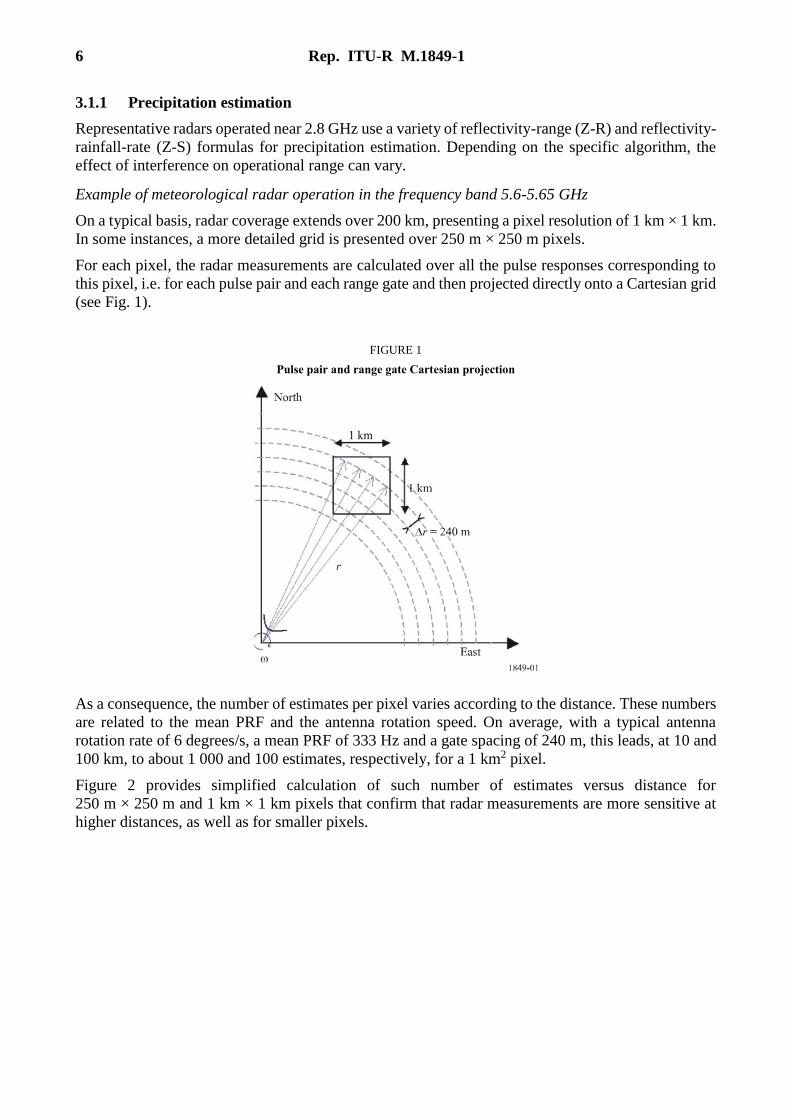
For each pixel, the radar measurements are calculated over all the pulse responses corresponding to

this pixel, i.e. for each pulse pair and each range gate and then projected directly onto a Cartesian grid

(see Fig. 1).

FIGURE 1

Pulse pair and range gate Cartesian projection

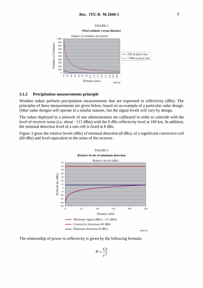
As a consequence, the number of estimates per pixel varies according to the distance. These numbers

are related to the mean PRF and the antenna rotation speed. On average, with a typical antenna

rotation rate of 6 degrees/s, a mean PRF of 333 Hz and a gate spacing of 240 m, this leads, at 10 and

100 km, to about 1 000 and 100 estimates, respectively, for a 1 km2 pixel.

Figure 2 provides simplified calculation of such number of estimates versus distance for

250 m × 250 m and 1 km × 1 km pixels that confirm that radar measurements are more sensitive at

higher distances, as well as for smaller pixels.

Rec. ITU-R M.1849-1 7

FIGURE 2

Pixel estimate versus distance

3.1.2 Precipitation measurements principle

Weather radars perform precipitation measurements that are expressed in reflectivity (dBz). The

principles of these measurements are given below, based on an example of a particular radar design.

Other radar designs will operate in a similar manner, but the signal levels will vary by design.

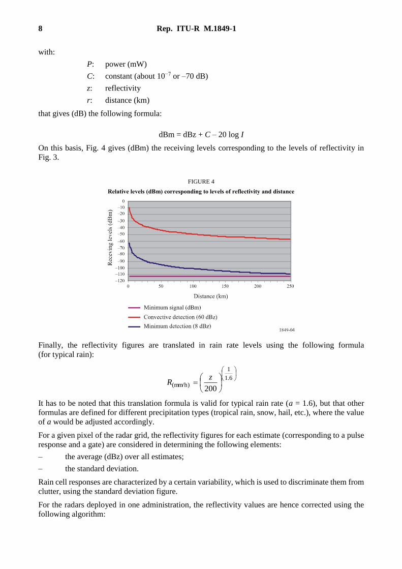
The radars deployed in a network of one administration are calibrated in order to coincide with the

level of receiver noise (i.e. about −113 dBm) with the 0 dBz reflectivity level at 100 km. In addition,

the minimal detection level of a rain cell is fixed at 8 dBz.

Figure 3 gives the relative levels (dBz) of minimal detection (8 dBz), of a significant convective cell

(60 dBz) and level equivalent to the noise of the receiver.

FIGURE 3

Relative levels of minimum detection

The relationship of power to reflectivity is given by the following formula:

2r

CzP

8 Rep. ITU-R M.1849-1

with:

P: power (mW)

C: constant (about 10−7 or –70 dB)

z: reflectivity

r: distance (km)

that gives (dB) the following formula:

dBm = dBz + C – 20 log I

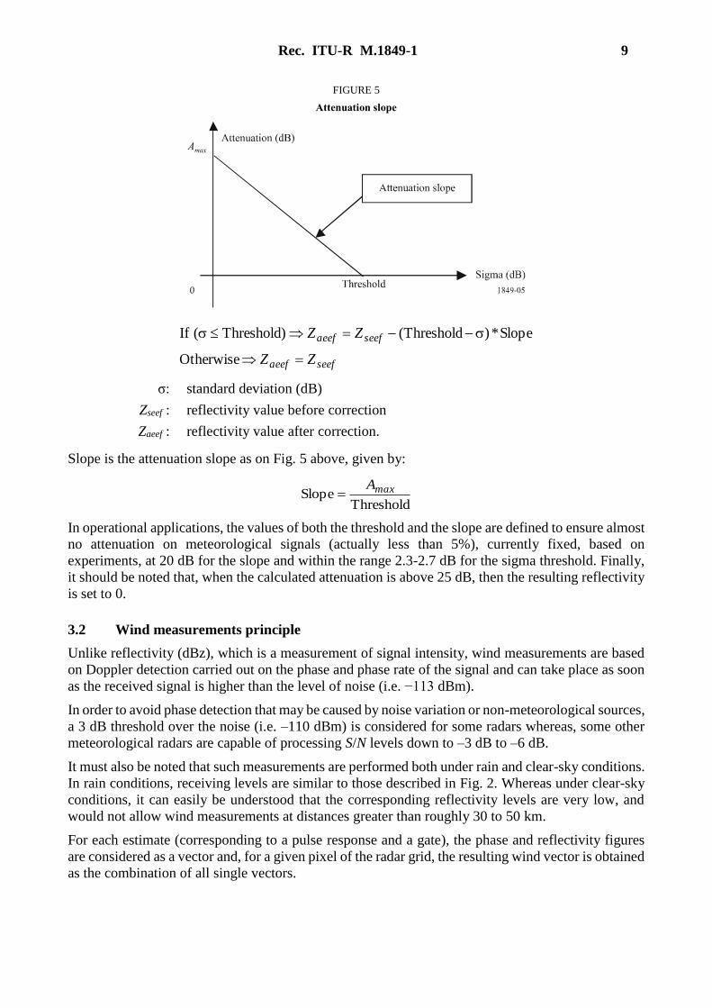
On this basis, Fig. 4 gives (dBm) the receiving levels corresponding to the levels of reflectivity in

Fig. 3.

FIGURE 4

Relative levels (dBm) corresponding to levels of reflectivity and distance

Finally, the reflectivity figures are translated in rain rate levels using the following formula

(for typical rain):

6.1

1

(mm/h)200

zR

It has to be noted that this translation formula is valid for typical rain rate (a = 1.6), but that other

formulas are defined for different precipitation types (tropical rain, snow, hail, etc.), where the value

of a would be adjusted accordingly.

For a given pixel of the radar grid, the reflectivity figures for each estimate (corresponding to a pulse

response and a gate) are considered in determining the following elements:

– the average (dBz) over all estimates;

– the standard deviation.

Rain cell responses are characterized by a certain variability, which is used to discriminate them from

clutter, using the standard deviation figure.

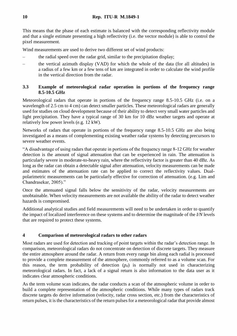
For the radars deployed in one administration, the reflectivity values are hence corrected using the

following algorithm:

Rec. ITU-R M.1849-1 9

FIGURE 5

Attenuation slope

seefaeef

seefaeef

ZZ

ZZ

Otherwise

Slope*)Threshold()Threshold( If

σ: standard deviation (dB)

Zseef : reflectivity value before correction

Zaeef : reflectivity value after correction.

Slope is the attenuation slope as on Fig. 5 above, given by:

Threshold

Slope maxA

In operational applications, the values of both the threshold and the slope are defined to ensure almost

no attenuation on meteorological signals (actually less than 5%), currently fixed, based on

experiments, at 20 dB for the slope and within the range 2.3-2.7 dB for the sigma threshold. Finally,

it should be noted that, when the calculated attenuation is above 25 dB, then the resulting reflectivity

is set to 0.

3.2 Wind measurements principle

Unlike reflectivity (dBz), which is a measurement of signal intensity, wind measurements are based

on Doppler detection carried out on the phase and phase rate of the signal and can take place as soon

as the received signal is higher than the level of noise (i.e. −113 dBm).

In order to avoid phase detection that may be caused by noise variation or non-meteorological sources,

a 3 dB threshold over the noise (i.e. –110 dBm) is considered for some radars whereas, some other

meteorological radars are capable of processing S/N levels down to –3 dB to –6 dB.

It must also be noted that such measurements are performed both under rain and clear-sky conditions.

In rain conditions, receiving levels are similar to those described in Fig. 2. Whereas under clear-sky

conditions, it can easily be understood that the corresponding reflectivity levels are very low, and

would not allow wind measurements at distances greater than roughly 30 to 50 km.

For each estimate (corresponding to a pulse response and a gate), the phase and reflectivity figures

are considered as a vector and, for a given pixel of the radar grid, the resulting wind vector is obtained

as the combination of all single vectors.

10 Rep. ITU-R M.1849-1

This means that the phase of each estimate is balanced with the corresponding reflectivity module

and that a single estimate presenting a high reflectivity (i.e. the vector module) is able to control the

pixel measurement.

Wind measurements are used to derive two different set of wind products:

– the radial speed over the radar grid, similar to the precipitation display;

– the vertical azimuth display (VAD) for which the whole of the data (for all altitudes) in

a radius of a few km or a few tens of km are integrated in order to calculate the wind profile

in the vertical direction from the radar.

3.3 Example of meteorological radar operation in portions of the frequency range

8.5-10.5 GHz

Meteorological radars that operate in portions of the frequency range 8.5-10.5 GHz (i.e. on a

wavelength of 2.5 cm to 4 cm) can detect smaller particles. These meteorological radars are generally

used for studies on cloud development because of their ability to detect very small water particles and

light precipitation. They have a typical range of 30 km for 10 dBz weather targets and operate at

relatively low power levels (e.g. 12 kW).

Networks of radars that operate in portions of the frequency range 8.5-10.5 GHz are also being

investigated as a means of complementing existing weather radar systems by detecting precursors to

severe weather events.

“A disadvantage of using radars that operate in portions of the frequency range 8-12 GHz for weather

detection is the amount of signal attenuation that can be experienced in rain. The attenuation is

particularly severe in moderate-to-heavy rain, where the reflectivity factor is greater than 40 dBz. As

long as the radar can obtain a detectable signal after attenuation, velocity measurements can be made

and estimates of the attenuation rate can be applied to correct the reflectivity values. Dual-

polarimetric measurements can be particularly effective for correction of attenuation. (e.g. Lim and

Chandrasekar, 2005).”

Once the attenuated signal falls below the sensitivity of the radar, velocity measurements are

unobtainable. When velocity measurements are not available the ability of the radar to detect weather

hazards is compromised.

Additional analytical studies and field measurements will need to be undertaken in order to quantify

the impact of localized interference on these systems and to determine the magnitude of the I/N levels

that are required to protect these systems.

4 Comparison of meteorological radars to other radars

Most radars are used for detection and tracking of point targets within the radar’s detection range. In

comparison, meteorological radars do not concentrate on detection of discrete targets. They measure

the entire atmosphere around the radar. A return from every range bin along each radial is processed

to provide a complete measurement of the atmosphere, commonly referred to as a volume scan. For

this reason, the term probability of detection (pd) is normally not used in characterizing

meteorological radars. In fact, a lack of a signal return is also information to the data user as it

indicates clear atmospheric conditions.

As the term volume scan indicates, the radar conducts a scan of the atmospheric volume in order to

build a complete representation of the atmospheric conditions. While many types of radars track

discrete targets do derive information (velocity, radar cross section, etc.) from the characteristics of

return pulses, it is the characteristics of the return pulses for a meteorological radar that provide almost

Rec. ITU-R M.1849-1 11

all the information. Unless the air is absolutely clear, meteorological radars receive and process

returns for almost all of the range bins along a radial.

The criteria for the operational evaluation of a typical weather radar system include:

a) technical aspects;

b) warning performance, and

c) quality and reliability of derived products.

Technical aspects include factors such as coverage at specific altitudes, spatial and temporal

resolution, sensitivity, Doppler coverage and radar availability. Warning performance can be viewed

as an objective measure, but is, in fact, directly linked to detection capability. The quality and the

reliability of the key derived products – reflectivity, mean radial velocity and spectral width-impact

a forecaster’s ability to provide hazardous weather warnings and timely and accurate forecasts.

4.1 Specificities with regards to protection criteria

For radars tracking discrete targets, an I/N = −6 dB, resulting in a 6% reduction of the range detection

is assumed acceptable. In fact, the signal received by these radars is proportional to 1/r4 (r being the

distance), and hence that the achievable free-space range is proportional to the 4th root of the resulting

SNR. An I/N = −6 dB corresponds to a 1 dB increase of the noise power and is a 1.26 factor in power.

Therefore, the resulting free-space range is reduced by a factor of 1/(1.261/4), or 1/1.06, i.e. a range

capability reduction of about 6%.

For meteorological radars, the situation is different for extended targets since, typically, precipitation

often fills the entire narrow radar beam. By using the radar equation developed in § 2.2, extended

targets result in a received signal proportional to 1/r² and a free-space range proportional to the square

root of the resulting SNR. In such cases, a similar acceptable 6% range capability reduction for

meteorological radars requires an interference factor in power of 1.12 (instead of 1.26 for other radar

types), corresponding to a noise increase of 0.5 dB and resulting in an I/N = −10 dB.

Detailed development and justification of this criteria is given in § 8.

4.2 Specificities with regards to emission schemes and scanning strategies

To ensure volume scan processing (typically in a range of 15 min), meteorological radars make use

of a variety of different emission schemes at different elevations, using sets of different pulse width,

PRF and rotation speeds, in so-called “scanning strategies”. There are unfortunately no typical

schemes, as they vary based on a number of factors, such as the radar capabilities and the radar

environment for the required meteorological products.

This has been confirmed following an enquiry on C-Band meteorological radars in Europe that

showed large ranges of different emission scheme parameters:

– Operational elevation ranging from 0° to 90°.

– Pulse width ranging from 0.5 to 2.5 μs (for operational radars). Existing radars are capable

of pulse width up to 3.3 μs for uncompressed pulses, whereas some radars use pulse

compression with pulse width of about 40 μs and expected 100 μs in the future.

– Pulse repetition frequency (PRF) ranging from 250 to 1 200 Hz (for operational radars).

Existing radars are capable of PRF up to 2 400 Hz.

– Rotation speed ranging from 1 to 6 rpm.

– Use on a given radar of different emission schemes mixing different pulse width and PRF,

and in particular the use of fixed, staggered or interleaved PRF (i.e. different PRF during a

single scheme).

12 Rep. ITU-R M.1849-1

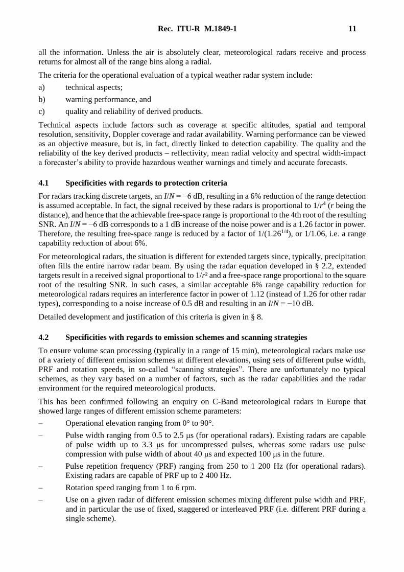
Some examples of such different emission schemes are provided below:

FIGURE 6

Fixed PRF

FIGURE 7

Staggered PRF

FIGURE 8

Double interleaved PRF (double PRT)

FIGURE 9

Triple interleaved PRF (triple PRT)

Rec. ITU-R M.1849-1 13

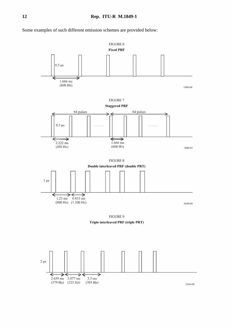
These different emission schemes are used on a number of radars in their scanning strategy, during

which, at different elevations and rotation speeds, one emission scheme is transmitted.

It has to be stressed that, from one radar to another, the PRF and pulse width values associated with

these example schemes vary within the ranges defined above. In addition, for a given scheme, pulse

widths can vary on a pulse to pulse basis.

Below is an example of such scanning strategy:

FIGURE 10

14 Rep. ITU-R M.1849-1

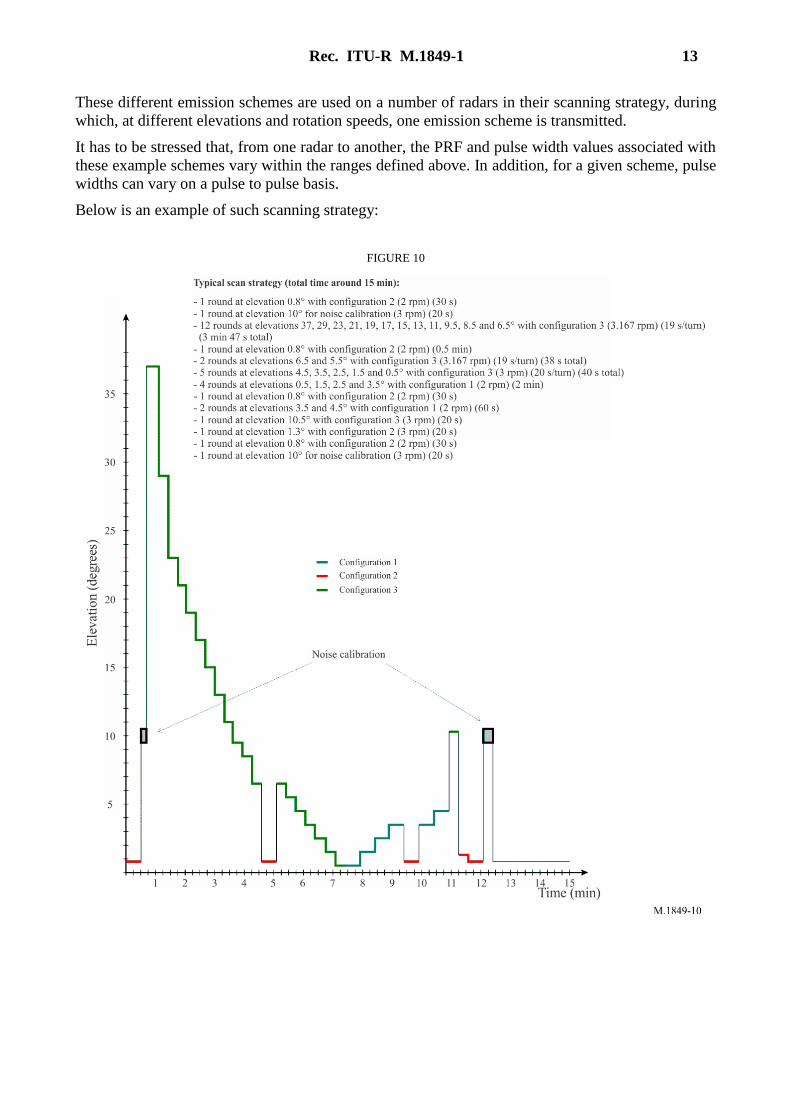
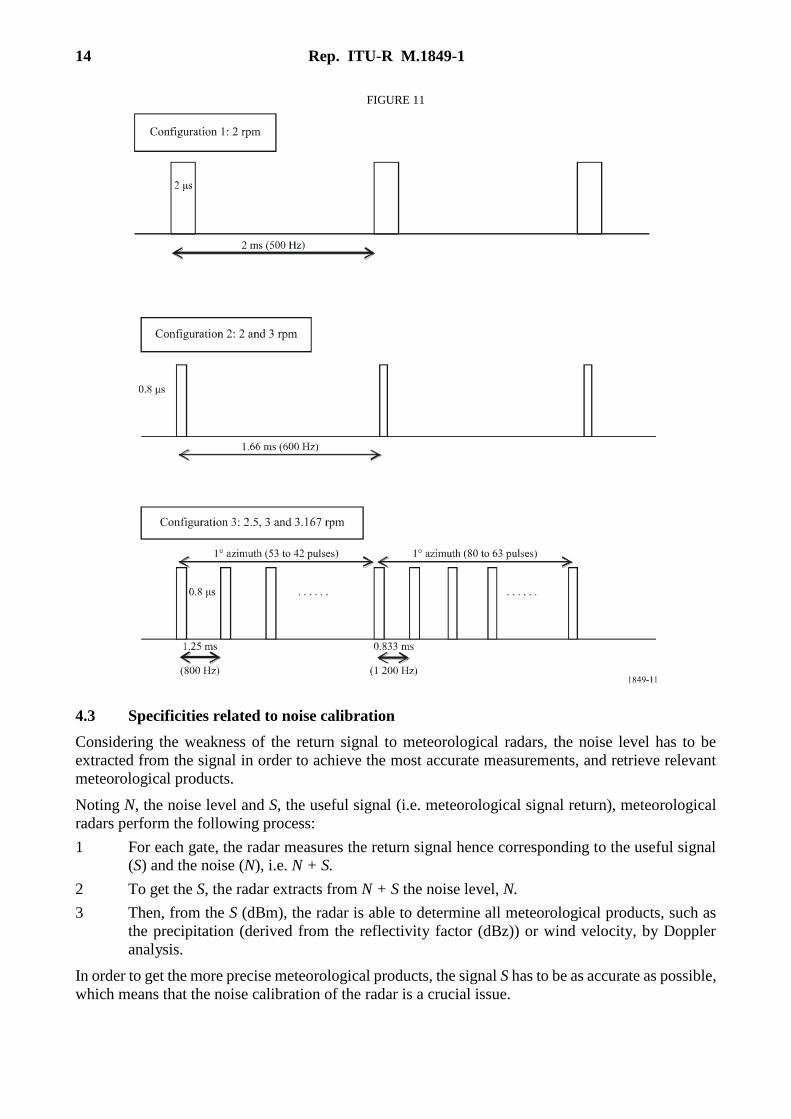
FIGURE 11

4.3 Specificities related to noise calibration

Considering the weakness of the return signal to meteorological radars, the noise level has to be

extracted from the signal in order to achieve the most accurate measurements, and retrieve relevant

meteorological products.

Noting N, the noise level and S, the useful signal (i.e. meteorological signal return), meteorological

radars perform the following process:

1 For each gate, the radar measures the return signal hence corresponding to the useful signal

(S) and the noise (N), i.e. N + S.

2 To get the S, the radar extracts from N + S the noise level, N.

3 Then, from the S (dBm), the radar is able to determine all meteorological products, such as

the precipitation (derived from the reflectivity factor (dBz)) or wind velocity, by Doppler

analysis.

In order to get the more precise meteorological products, the signal S has to be as accurate as possible,

which means that the noise calibration of the radar is a crucial issue.

Rec. ITU-R M.1849-1 15

This noise calibration, also called “Zero Check”, is therefore performed on a regular basis, either

during regular radar emissions (by estimation) or during specific periods of time (see the example

scanning strategy above) during which the noise is measured.

In many cases, this noise measurement is performed without any radar emission (this could in

particular have an impact on the design of certain radio systems that aim at detecting radar signal to

mitigate interference).

In all cases, interference received during the noise check calibration will corrupt all data collection

until the next interference free calibration is performed.

5 Operational modes for meteorological radar

The typical Doppler meteorological radar operates in two user selectable modes: Clear air mode and

precipitation mode. Clear air mode requires manual selection by the user. The precipitation mode

may be selected manually at any time during operation or can be automatically operated whenever

the weather radar detects precipitation (based upon pre-determined values and area coverage of

reflectivity). In general, meteorological radars take advantage of both modes.

5.1 Clear air mode

Clear air mode provides meteorological radars the ability to detect early signs of precipitation activity.

There exist certain variables in low-level velocity and air density that allow for detection of potential

precipitation. The radar utilizes a slow scan rate, coupled with a low pulse repetition frequency (PRF),

to employ a high sensitivity capability. This high sensitivity is ideal for very subtle changes in

atmospheric conditions at long ranges. The clear air mode is especially useful when there is little to

no convective activity within the transmit range of the radar, and is ideally suited for detecting the

signs of developing thunderstorms or other types of severe weather.

Meteorological radar’s high sensitivity is due to the volume scan pattern within the clear air mode.

By selecting a pattern in the clear air mode; the radar antenna is capable of dwelling for an extended

period in any given volume of space and receives multiple returns, while allowing operation at a

lower S/N. The use of a wide pulse width and a low PRF provides approximately 8 dB echo power

for a given dBz of reflectivity.

5.2 Precipitation mode

The precipitation mode performs a distinctly different purpose than the clear air mode. The scan rate

for the precipitation mode is a function of the elevation angle. This dependence allows for the highest

number of elevation angles possible in sampling the total radar volume. The precipitation mode takes

advantage of multiple volume coverage patterns (VCPs) to implement different types of scan

strategies (see example in § 4.2) with different elevation sampling. Weather events normally

monitored in the precipitation mode are associated with the development of precipitation involving

convective storms (rain showers, hail, severe thunderstorms, tornadoes, etc.) and large-scale synoptic

systems.

6 Meteorological radar data products

To provide a better understanding of meteorological radars for the purpose of interference analysis

and spectrum management, two categories of meteorological radar data products must be considered:

base data products and derived data products.

16 Rep. ITU-R M.1849-1

6.1 Conventional meteorological radar base data products

A Doppler meteorological radar generates three categories of base data products from the signal

returns: base reflectivity, mean radial velocity and spectrum width. All higher-level products are

generated from these three base products. The base product accuracy is often specified as a primary

performance requirement for radar design. Without the required accuracy at this low level, the higher-

level derived product accuracy cannot be achieved. In a previous ITU-R study on meteorological

radars, the impact of permissible interference on the base product data was used as a metric for the

protection criteria. For example, a representative radar with the base data accuracies shown in Table

1 was used in a study to determine the interference-to-noise ratio that caused the radar to no longer

meet its design requirements. Section 8.3 and Annex 1 of Report ITU-R M.2136 address the details

of determining meteorological radar protection criteria.

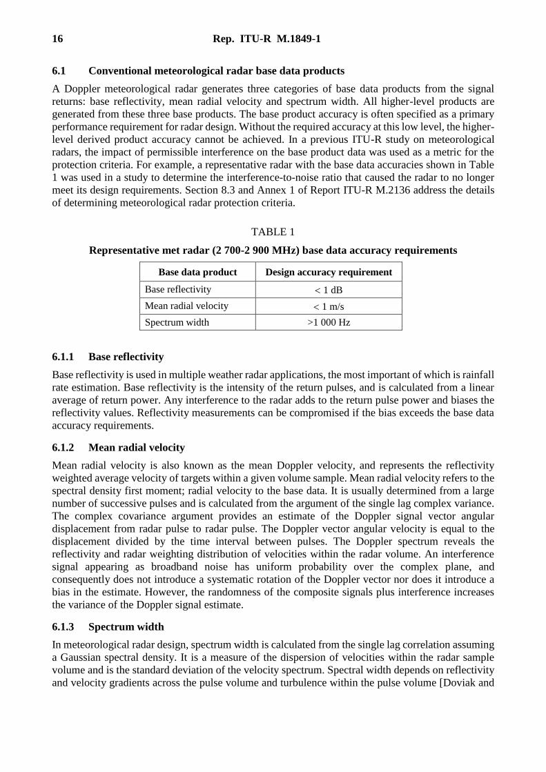
TABLE 1

Representative met radar (2 700-2 900 MHz) base data accuracy requirements

Base data product Design accuracy requirement

Base reflectivity 1 dB

Mean radial velocity 1 m/s

Spectrum width >1 000 Hz

6.1.1 Base reflectivity

Base reflectivity is used in multiple weather radar applications, the most important of which is rainfall

rate estimation. Base reflectivity is the intensity of the return pulses, and is calculated from a linear

average of return power. Any interference to the radar adds to the return pulse power and biases the

reflectivity values. Reflectivity measurements can be compromised if the bias exceeds the base data

accuracy requirements.

6.1.2 Mean radial velocity

Mean radial velocity is also known as the mean Doppler velocity, and represents the reflectivity

weighted average velocity of targets within a given volume sample. Mean radial velocity refers to the

spectral density first moment; radial velocity to the base data. It is usually determined from a large

number of successive pulses and is calculated from the argument of the single lag complex variance.

The complex covariance argument provides an estimate of the Doppler signal vector angular

displacement from radar pulse to radar pulse. The Doppler vector angular velocity is equal to the

displacement divided by the time interval between pulses. The Doppler spectrum reveals the

reflectivity and radar weighting distribution of velocities within the radar volume. An interference

signal appearing as broadband noise has uniform probability over the complex plane, and

consequently does not introduce a systematic rotation of the Doppler vector nor does it introduce a

bias in the estimate. However, the randomness of the composite signals plus interference increases

the variance of the Doppler signal estimate.

6.1.3 Spectrum width

In meteorological radar design, spectrum width is calculated from the single lag correlation assuming

a Gaussian spectral density. It is a measure of the dispersion of velocities within the radar sample

volume and is the standard deviation of the velocity spectrum. Spectral width depends on reflectivity

and velocity gradients across the pulse volume and turbulence within the pulse volume [Doviak and

Rec. ITU-R M.1849-1 17

Zrnic, 1984]2. There is no averaging of samples used in spectrum width calculations. There is

however an accumulation of the real and imaginary parts of the sample series, i.e. the samples taken

over the radial.

6.2 Dual polarization meteorological radar products

6.2.1 Differential reflectivity

Differential reflectivity is a product that is associated with polarimetric meteorological radars, and is

a ratio of the reflected horizontal and vertical power returns. Among other things, it is a good indicator

of drop shape. In turn the shape is a good estimate of average drop size.

6.2.2 Correlation coefficient

Correlation coefficient is a polarimetric meteorological radar product and is a statistical correlation

between the reflected horizontal and vertical power returns. The correlation coefficient describes the

similarities in the backscatter characteristics of the horizontally and vertically polarized echoes. It is

a good indicator of regions where there is a mixture of precipitation types, such as rain and snow.

6.2.3 Linear depolarization ratio

Another polarimetric radar product is linear depolarization ratio, which is a ratio of a vertical power

return from a horizontal pulse or a horizontal power return from a vertical pulse. It, too, is a good

indicator of regions where mixtures of precipitation types occur.

6.2.4 Specific differential phase

The specific differential phase is also a polarimetric meteorological radar product. It is a comparison

of the returned phase difference between the horizontal and vertical pulses. This phase difference is

caused by the difference in the number of wave cycles (or wavelengths) along the propagation path

for horizontal and vertically polarized waves. It should not be confused with the Doppler frequency

shift, which is caused by the motion of the cloud and precipitation particles. Unlike the differential

reflectivity, correlation coefficient and linear depolarization ratio, which are all dependent on

reflected power, the specific differential phase is a “propagation effect”. It is also a very good

estimator of rain rate.

6.3 Derived data products

Using the base data products, the processor produces higher-level derived data products for the radar

user. This text will not address the derived data products in detail as the products vary from radar to

radar and the number of products is quite large. To ensure accuracy of the derived data products, the

base data products need to be accurately maintained.

7 Antenna pattern and antenna dynamics

Meteorological radars typically use parabolic reflector antennas that produce a pencil beam antenna

pattern. Standard ITU antenna patterns for parabolic antennas are not applicable to antennas used for

meteorological radars, as the generated main beam pattern is often much wider than the actual pencil

beam pattern. Use of a broader antenna pattern often provides sharing results indicating more

significant interference problems than an accurate antenna pattern.

2 DOVIAK, R. J. and ZRNIC. D. S. [1984] Doppler and Weather Observations. Academic Press, Inc. San

Diego, United States of America.

18 Rep. ITU-R M.1849-1

7.1 Volume scan antenna movement

The horizontal and vertical coverage required for a volume scan to produce an elevation cut, is

achieved by rotating the antenna in the horizontal plane at a constant elevation angle The antenna

elevation is increased by a preset amount after each elevation cut. The lowest elevation cut is typically

in the range of 0º to 1º, and the highest elevation is in the 20º to 30º range, though some applications

can use elevations up to 60º. Rotation speed of the antenna varies depending on weather conditions

and the product required at the time. The rotation speed as well as range of elevation, intermediate

elevation steps, and pulse repetition frequency, is adjusted for optimum performance. Slow antenna

rotation provides a long per-radial dwell time for maximum sensitivity.

High antenna rotation speed allows the operator to generate a volume scan in a short period of time

when it is desirable to cover the entire volume as quickly as possible. Variation of the elevation steps

and rotation speed can result in volume scan acquisition times ranging from one minute up to 15 min.

The long periods of time for a complete volume scan, compared to other radars that rotate at a constant

elevation, make it necessary to run dynamic simulations much longer to obtain a statistically

significant sampling of results.

7.2 Other antenna movement strategies

Meteorological radars also use other antenna movement strategies for special applications and

research. Sector scans are used to get part of an elevation cut. Sector volume scans perform a volume

scan for a fraction of the 360º azimuth where the antenna takes multiple elevations cuts. The third

mode holds the antenna at a constant azimuth and elevation to monitor a specific point in the

atmosphere. All three strategies allow the radar operator to concentrate on a specific part of the

atmosphere.

7.3 Antenna patterns

Whenever possible, sharing studies should be conducted using the actual antenna pattern of the radar

under study. But in cases where actual antenna pattern data is not available, a generic set of curves or

formulas for deriving representative antenna characteristics would be beneficial.

Three mathematical models for radar antenna patterns are currently used in interference analysis with

radars as given in Recommendations ITU-R F.1245, ITU-R M.1652 and ITU-R F.699. Although

representative of parabolic antennas, these Recommendations tend to overestimate the beamwidth of

a pencil beam antenna pattern, similar to that generally used by meteorological radars.

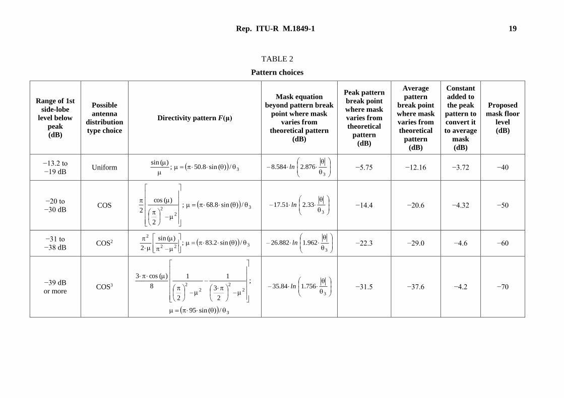
Currently there are no defined radar antenna radiation pattern equations within ITU-R to represent

such pencil beam antennas. If required, generalized antenna radiation pattern models, as outlined in

Table 2, could be used, in the absence of measured data, in interference analyses involving single and

multiple interferers, see also Recommendation ITU-R M.1851. θ3 is the half power beam-width

(degrees).

Rep. ITU-R M.1849-1 19

TABLE 2

Pattern choices

Range of 1st

side-lobe

level below

peak

(dB)

Possible

antenna

distribution

type choice

Directivity pattern F(μ)

Mask equation

beyond pattern break

point where mask

varies from

theoretical pattern

(dB)

Peak pattern

break point

where mask

varies from

theoretical

pattern

(dB)

Average

pattern

break point

where mask

varies from

theoretical

pattern

(dB)

Constant

added to

the peak

pattern to

convert it

to average

mask

(dB)

Proposed

mask floor

level

(dB)

−13.2 to

−19 dB Uniform 3/)(sin8.50;

)(sin

3

876.2584.8– ln −5.75 −12.16 −3.72 −40

−20 to

−30 dB COS 3

22

/)(sin8.68;

–2

)(cos

2

3

33.251.17– ln −14.4 −20.6 −4.32 −50

−31 to

−38 dB COS2 322

2

/)(sin2.83;–

)(sin

2

3

962.1882.26– ln −22.3 −29.0 −4.6 −60

−39 dB

or more COS3

;

–2

3

1–

–2

1

8

)(cos3

22

22

3/)(sin95

3

756.184.35– ln −31.5 −37.6 −4.2 −70

20 Rec. ITU-R M.1849-1

8 Effects of interference and solar noise on meteorological radars

Determining the effects of interference on radars used for detecting point targets is fairly

straightforward. Testing can be accomplished by injecting simulated known targets into the radar,

and visually determining the interference level at which the targets are lost or false targets are

generated. Visual inspection of the derived data products from a meteorological radar volume scan,

as displayed on an operator console, does not provide obvious indication whether interference has

degraded the radar’s performance. For example, if interference were to cause a 1 dB bias in the base

reflectivity data, it will not be obvious on a graphical display of rainfall. However, if the interference

is present for a large part of the volume scan, each and every range bin will be biased within the

affected volume. The cumulative effect is a significant overestimation of rainfall in a geographic

region.

All meteorological radars experience sun strobes during the periods of sunrise and sunset. A sun

strobe is caused whenever the antenna main beam aligns with the sun during a volume scan. The effect

of sun strobes, in the particular case of meteorological radars, results in the total loss of data along

one to two radials in the direction of the sun. It should be noted that the predictability of sun strobes

may allow for the calibration in azimuth of the radars pointing direction.

The effects of the sun are undesirable, but predictable. With other forms of interference and noise the

location and intensity are unknown and cannot be predicted or easily addressed through processing

or operator interpretation.

Base products are affected by interference in two different ways. First, values can be biased which

decreases the accuracy of the system, and second, the variance of the outputs can be affected. In the

presence of interference, reflectivity is sensitive to bias, mean radial velocity is sensitive to variance

errors, and spectrum width is affected by both bias and variance errors. For spectrum width, the errors

due to biasing are more significant than the errors due to variance because the bias, or offset,

represents a velocity measurement error, while the variance represents the uncertainty of the

velocities measured.

8.1 Impact of interference on modes of operation

In the clear air mode, the signal-to-noise-ratio of the returns is the lowest, and the data is most

vulnerable to corruption by interference. Typically when operating in clear air mode,

the meteorologist is looking for the initial signs of convection, as it may develop into severe weather

and possibly tornadoes. Detection of convection requires the detection of fine lines caused by

scatterers, indicating discontinuity boundaries that initiate convection. The width of these areas of

convection is often on the order of one to two radials in width, and interference along those radials

would prevent detection. Therefore interference for even very brief periods of time could result in

loss of detection of forming severe weather. If that information is lost along a critical radial during

a volume scan, detection will be delayed on the order of 10 min until the volume scan returns the

antenna position to that area of the atmosphere.

The precipitation mode is the more demanding mode in terms of communications, radar product

generation, and user processing and display. For the precipitation mode, nearly all of the algorithms

rely on the base data of reflectivity, mean velocity, and spectrum width to generate derived products

for use by the operator.

8.2 Impact of interference upon base products

Base products are affected by interference in two different ways. First, values can be biased, which

decreases the accuracy of the system, and second, the variance of the outputs can be affected. In the

Rec. ITU-R M.1849-1 21

presence of interference, reflectivity is sensitive to bias, mean radial velocity is sensitive to variance

errors, and spectrum width is affected by both bias and variance errors. For spectrum width, the errors

due to biasing are more significant than the errors due to variance because the bias, or offset,

represents a velocity measurement error while the variance represents the uncertainty of the velocities

measured.

Reflectivity is calculated from a linear average of power. In the some meteorological radars

reflectivity estimates are formed for range bins that span 250 m in depth by one radial wide

(approximately 1.0º in azimuth). These systems average range bins to produce a reflectivity estimate

output at specified intervals. This averaging of four to one can further mitigate effects of interference

occurring on a single pulse. Next generation meteorological radar systems have plans to add a “super-

resolution” reflectivity product, which will eliminate the averaging and produce reflectivity estimates

at 250-m intervals. Additionally, the radial will be reduced to half (0.5º), which will use only half the

samples. The total affect will be to reduce the sample size by eight. Thus, interference may be more

pronounced in the “super resolution” reflectivity product than in current estimates.

For Doppler moments the interference effects are non-linear. Velocity is calculated from the complex

covariance argument and spectrum width from the autocorrelation. A mix of signal and interference

does not scale linearly, as with the average for reflectivity. These estimates result from accumulation

of signal measurements consisting of both magnitude and phase angle information. Interfering

sources would likely have random phases with respect to the coherent met radar signal, and their

contribution to the estimate accuracy is difficult to predict.

In terms of spectrum width, interference introduces both a bias and an increase in the variance of the

spectrum width estimation. The bias in the estimation is more detrimental than the increase in

variance.

Measurement errors need to be specified so that radar observations can be properly assimilated for

numerical weather prediction. There are two related aspects to this problem:

1 errors in the original measurements within each radar pulse volume that are in part caused by

interfering signals, and

2 representative of the radar data estimates used in the assimilation process.

For radial velocities, the first error source depends on the strength of the return signal and the spread

or width of the Doppler velocity spectrum. Spectral width in turn depends mainly on reflectivity and

velocity gradients within and across the pulse volume and turbulence within the pulse volume

[Doviak and Zrnic, 1984]. Estimation of these errors is complicated by the fact that the components

needed for reliable error estimation are themselves only measured and, therefore, has inherent

uncertainties.

The concept has been raised that, for a given range resolution cell, meteorological radars average

multiple pulse returns over the dwell time of a radial. It has been suggested that in the case where

interference occurs for a short part of the radial dwell time, the effect of the interference will be

averaged with the interference-free pulse returns, thereby reducing the effects of the interference. For

instance, if the radar operates at an interference to noise ratio well below −10 dB, but the −10 dB is

violated for a short period of time (small percentage of radial dwell time), the effect of the interference

will then be averaged with the interference free-returns. If the –10 dB I/N is violated, but not by a

high level of interference, the possible result is that the reflectivity bias of the averaged returns may

stay within the design objective of the given radar. Unfortunately, this approach can only be effective

if the interfering signal or signals are coherent over the dwell time. Since this does not happen often,

averaging techniques may not be the most effective way of mitigating the effects of interference upon

Doppler moments. However, with the exception of meteorological radars that employ spectral

processing, averaging can be an effective way to mitigate interference given that the average

interference over the dwell time has an I/N of less than −10 dB.

22 Rec. ITU-R M.1849-1

As explained in § 4.2 above, an I/N = −6 dB leads to a range capability reduction of about 12% for

meteorological radars and 6% for other radars. On the other hand, such 6% range capability reduction

(that also relates to a 11% degradation in area coverage) would relate to a noise increase of about

0.5 dB for meteorological radars, and hence corresponds to an I/N = −10 dB. Testing in support of

such I/N of −10 dB figure for constant interference were recently performed (see Annex 2 of Report

ITU-R M.2136).

The impact of interference upon polarimetric or dual-polarization meteorological radar products, such

as differential reflectivity, correlation coefficient, linear depolarization ratio and specific differential

phase, needs additional study from both a mathematical and a measurement based perspective in order

to quantify the protection criteria levels that are required to assure that polarimetric radar products

are not compromised by interference.

It should be concluded that interference to meteorological radars should be minimized, with the

objective of mitigating or preventing all interference. Unlike communication systems that use

redundancy and error correction, meteorological radars cannot reacquire lost information. However,

when considering the use of radar characteristics for ITU-R sharing studies, other factors do need to

be considered and are addressed in the following sections.

8.3 Mathematical derivation of meteorological radar protection criteria

Weather radars perform three basic measurements, which, in conjunction with operator information,

are used to derive meteorological products. The three base products from which other products are

derived are volume reflectivity, radial velocity and spectrum width.

Section 2 of Annex 1 of Report ITU-R M.2136 provides a detailed discussion of mathematically

deriving meteorological radar interference criteria for these three products, further supported by test

results to validate the derivations.

While it is convenient, and often done, a single protection criteria value cannot be accurately applied

to all meteorological radars operating in a single band. Meteorological radars are designed with

varying performance objectives, where those objectives are optimized for specific meteorological

conditions. The base product accuracy and the radar minimum signal-to-noise ratio, S/N, vary from

radar application to radar application. The lower the minimum S/N used by the radar, the lower the

required protection criteria.

Signal processing removes many of the effects of radar system noise from the reflectivity and

spectrum width measurements; as a result, some systems can provide estimates of these products for

signal levels that are below the receivers’ noise level. The radars’ operator selects the signal to noise

threshold3, SNR, which, in some systems, can have a range of −12 dB to 6 dB.

The typical meteorological radar used in the examples developed in § 2 of Annex 1 of Report

ITU-R M.2136 provides useful measurements down to an SNR of −3 dB. Interference at this signal

level and above will degrade the quality of the base products. This highlights the need to establish an

I/N ratio that protects the integrity of these products.

Given the technical specifications and base data accuracy requirements of any given meteorological

radar one can derive the theoretical I/Ns which are required in order to assure that the base products

are not compromised in terms of bias and variance.

3 The SNR threshold is the lowest level for which the return signal is processed.

Rec. ITU-R M.1849-1 23

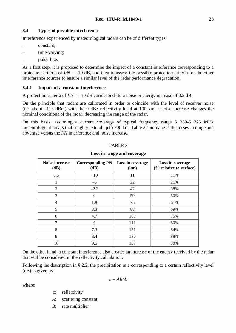
8.4 Types of possible interference

Interference experienced by meteorological radars can be of different types:

– constant;

– time-varying;

– pulse-like.

As a first step, it is proposed to determine the impact of a constant interference corresponding to a

protection criteria of I/N = –10 dB, and then to assess the possible protection criteria for the other

interference sources to ensure a similar level of the radar performance degradation.

8.4.1 Impact of a constant interference

A protection criteria of I/N = –10 dB corresponds to a noise or energy increase of 0.5 dB.

On the principle that radars are calibrated in order to coincide with the level of receiver noise

(i.e. about –113 dBm) with the 0 dBz reflectivity level at 100 km, a noise increase changes the

nominal conditions of the radar, decreasing the range of the radar.

On this basis, assuming a current coverage of typical frequency range 5 250-5 725 MHz

meteorological radars that roughly extend up to 200 km, Table 3 summarizes the losses in range and

coverage versus the I/N interference and noise increase.

TABLE 3

Loss in range and coverage

Noise increase

(dB)

Corresponding I/N

(dB)

Loss in coverage

(km)

Loss in coverage

(% relative to surface)

0.5 –10 11 11%

1 –6 22 21%

2 –2.3 42 38%

3 0 59 50%

4 1.8 75 61%

5 3.3 88 69%

6 4.7 100 75%

7 6 111 80%

8 7.3 121 84%

9 8.4 130 88%

10 9.5 137 90%

On the other hand, a constant interference also creates an increase of the energy received by the radar

that will be considered in the reflectivity calculation.

Following the description in § 2.2, the precipitation rate corresponding to a certain reflectivity level

(dB) is given by:

z = AR^B

where:

z: reflectivity

A: scattering constant

B: rate multiplier

24 Rec. ITU-R M.1849-1

and

z = 10 log z (dBz)

where:

dBz: reflectivity (dB).

Rearranging terms and solving for R yields the following equation:

6.1

1

10

dBz

)(mm/h200

10R

Assuming a constant energy increase, C, the resulting rain rate is:

6.1

1

10

dBz

)mm/h(200

10

C

R

The rain rate increase in percentage is then a constant that is given by:

110100)( 16(mm/h)

C

Rp

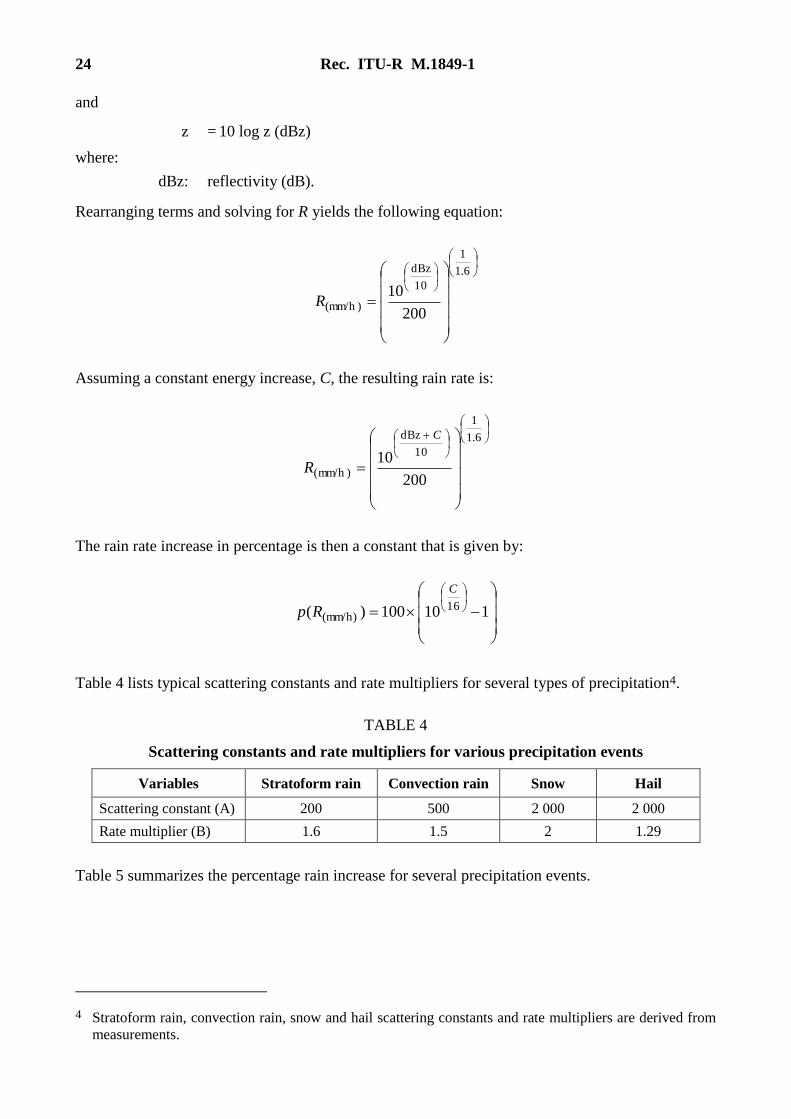
Table 4 lists typical scattering constants and rate multipliers for several types of precipitation4.

TABLE 4

Scattering constants and rate multipliers for various precipitation events

Variables Stratoform rain Convection rain Snow Hail

Scattering constant (A) 200 500 2 000 2 000

Rate multiplier (B) 1.6 1.5 2 1.29

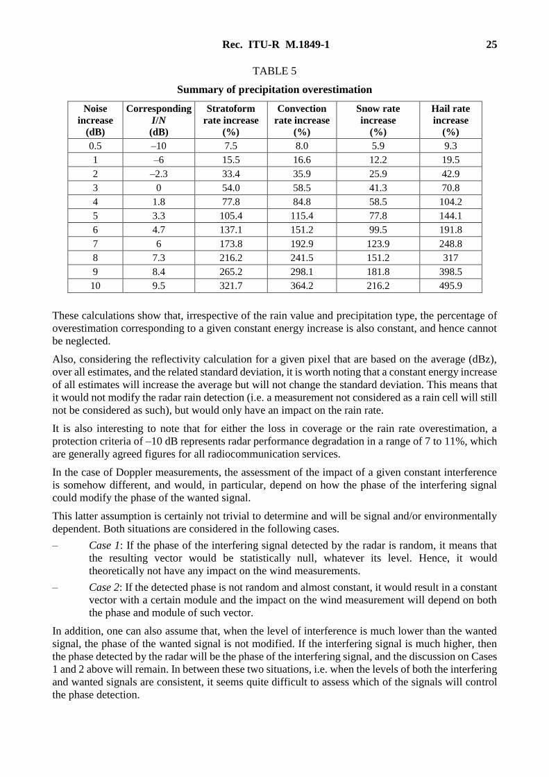
Table 5 summarizes the percentage rain increase for several precipitation events.

4 Stratoform rain, convection rain, snow and hail scattering constants and rate multipliers are derived from

measurements.

Rec. ITU-R M.1849-1 25

TABLE 5

Summary of precipitation overestimation

Noise

increase

(dB)

Corresponding

I/N

(dB)

Stratoform

rate increase

(%)

Convection

rate increase

(%)

Snow rate

increase

(%)

Hail rate

increase

(%)

0.5 –10 7.5 8.0 5.9 9.3

1 –6 15.5 16.6 12.2 19.5

2 –2.3 33.4 35.9 25.9 42.9

3 0 54.0 58.5 41.3 70.8

4 1.8 77.8 84.8 58.5 104.2

5 3.3 105.4 115.4 77.8 144.1

6 4.7 137.1 151.2 99.5 191.8

7 6 173.8 192.9 123.9 248.8

8 7.3 216.2 241.5 151.2 317

9 8.4 265.2 298.1 181.8 398.5

10 9.5 321.7 364.2 216.2 495.9

These calculations show that, irrespective of the rain value and precipitation type, the percentage of

overestimation corresponding to a given constant energy increase is also constant, and hence cannot

be neglected.

Also, considering the reflectivity calculation for a given pixel that are based on the average (dBz),

over all estimates, and the related standard deviation, it is worth noting that a constant energy increase

of all estimates will increase the average but will not change the standard deviation. This means that

it would not modify the radar rain detection (i.e. a measurement not considered as a rain cell will still

not be considered as such), but would only have an impact on the rain rate.

It is also interesting to note that for either the loss in coverage or the rain rate overestimation, a

protection criteria of –10 dB represents radar performance degradation in a range of 7 to 11%, which

are generally agreed figures for all radiocommunication services.

In the case of Doppler measurements, the assessment of the impact of a given constant interference

is somehow different, and would, in particular, depend on how the phase of the interfering signal

could modify the phase of the wanted signal.

This latter assumption is certainly not trivial to determine and will be signal and/or environmentally

dependent. Both situations are considered in the following cases.

– Case 1: If the phase of the interfering signal detected by the radar is random, it means that

the resulting vector would be statistically null, whatever its level. Hence, it would

theoretically not have any impact on the wind measurements.

– Case 2: If the detected phase is not random and almost constant, it would result in a constant

vector with a certain module and the impact on the wind measurement will depend on both

the phase and module of such vector.

In addition, one can also assume that, when the level of interference is much lower than the wanted

signal, the phase of the wanted signal is not modified. If the interfering signal is much higher, then

the phase detected by the radar will be the phase of the interfering signal, and the discussion on Cases

1 and 2 above will remain. In between these two situations, i.e. when the levels of both the interfering

and wanted signals are consistent, it seems quite difficult to assess which of the signals will control

the phase detection.

26 Rec. ITU-R M.1849-1

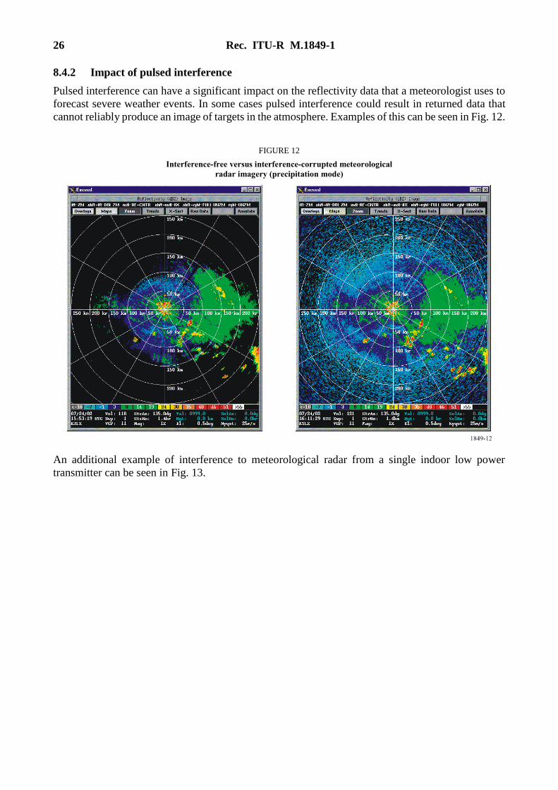
8.4.2 Impact of pulsed interference

Pulsed interference can have a significant impact on the reflectivity data that a meteorologist uses to

forecast severe weather events. In some cases pulsed interference could result in returned data that

cannot reliably produce an image of targets in the atmosphere. Examples of this can be seen in Fig. 12.

FIGURE 12

Interference-free versus interference-corrupted meteorological

radar imagery (precipitation mode)

An additional example of interference to meteorological radar from a single indoor low power

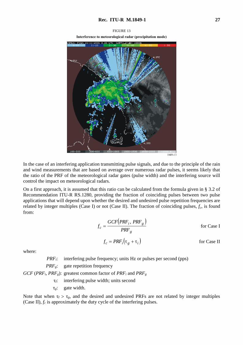
transmitter can be seen in Fig. 13.

Rec. ITU-R M.1849-1 27

FIGURE 13

Interference to meteorological radar (precipitation mode)

In the case of an interfering application transmitting pulse signals, and due to the principle of the rain

and wind measurements that are based on average over numerous radar pulses, it seems likely that

the ratio of the PRF of the meteorological radar gates (pulse width) and the interfering source will

control the impact on meteorological radars.

On a first approach, it is assumed that this ratio can be calculated from the formula given in § 3.2 of

Recommendation ITU-R RS.1280, providing the fraction of coinciding pulses between two pulse

applications that will depend upon whether the desired and undesired pulse repetition frequencies are

related by integer multiples (Case I) or not (Case II). The fraction of coinciding pulses, fc, is found

from:

g

gic

PRF

PRFPRFGCFf

, for Case I

igic PRFf for Case II

where:

PRFi: interfering pulse frequency; units Hz or pulses per second (pps)

PRFg: gate repetition frequency

GCF (PRFi, PRFg): greatest common factor of PRFi and PRFg

τI: interfering pulse width; units second

τg: gate width.

Note that when τI τg, and the desired and undesired PRFs are not related by integer multiples

(Case II), fc is approximately the duty cycle of the interfering pulses.

28 Rec. ITU-R M.1849-1

On this basis, in order to maintain the same level of degradation (about 10%) as for a constant

interference where I/Nconstant = –10 dB applies, it is assumed that the maximum I/N related to a pulse

interference could be given by:

cconstantpulse fI/NI/N log10–

In fact, if the fraction of coinciding pulses is 0.5, meaning that one of two radar estimates will be

polluted by the interference, and that the interfering signal is doubled (+3 dB) compared to the

situation pertaining to an I/N = −10 dB, it is obvious that the average calculated by the radar will be

the same.

On the other hand, the standard deviation will increase which will, in some cases, make

a non-meteorological event be taken as a rain situation. In this case, it is assumed that 10%

degradation would be acceptable, but this still needs to be validated and justified by calculation as

well as by testing.

It has to be noted that the above principle that higher I/N corresponding to peak power of pulsed

interference can be accepted by meteorological radars has been confirmed by recent testing (see

Annex 2 of Report ITU-R M.2136). Even though the above formula was not fully validated in all

cases, it is hence assumed to represent a relevant approach. Further analysis to determine the

relationship between victim and interferer signal characteristics (PRF and pulse width) could,

however, be appropriate.

8.4.2.1 An alternative method for deriving the I/N levels for pulsed interference

Meteorological radars process signal returns to measure precipitation and wind patterns.

The processing involves collecting and processing base products; reflectivity, mean radial velocity,

and spectrum width. In simplest terms, the radar averages a sample of signal returns to derive the

estimates needed for production of meteorological products. The averaging function will provide the

meteorological radar the ability to process higher pulsed interference levels relative to CW or noise-

like interference signals.

Meteorological radars process multiple pulse returns falling within a range bin to form a sample of

a size defined by the user. The multiple pulse returns forming a range bin sample are averaged to

derive the range bin estimate. The proposed EESS systems and meteorological radars operate on

significantly different pulse repetition frequencies, so the likelihood of more than one interfering

pulse falling within a single meteorological radar range bin sample set is small, given a small sample

size. The approach is to determine the maximum level of a single pulse that will not corrupt the

average of the sample size beyond the base data product performance objectives of the radar.

Determination of a protection criterion requires an understanding of the radar’s receiver noise level,

the minimum signal-to-noise ratio used for processing, and the radar’s base products (reflectivity,

man radial velocity and spectrum width) accuracy requirements. Since a variety of meteorological

radars are operated in the frequency band, some assumptions must be made. The radar used in the

analysis has a receiver noise floor of –110 dBm at the narrowest IF bandwidth.

The minimum signal-to-noise ratio is probably the most difficult value to establish without reference

to specific radars. For radars operated in the frequency band 2 700-2 900 MHz signal-to-noise ratios

of 0 to 3 dB are typical, since the lower frequency radars are generally operated for detection at long

ranges. Meteorological radars operated in the frequency band 9 300-9 500 MHz are generally used

for shorter-range, higher-resolution detection, and may operate at higher minimum signal-to-noise

ratios. For this analysis, an S/N of +3 dB and a noise floor of –110 dBm result in the values of the

base data product accuracy requirements which are shown in Table 6.

Rec. ITU-R M.1849-1 29

TABLE 6

Data accuracy requirements

Base data accuracy requirements

Reflectivity estimate 1 dB

Velocity estimate 1 m/s

Spectrum width estimate 1 000 Hz

As shown in Table 6, the maximum reflectivity bias limit for the meteorological radar used in this

example is assumed to be 1 dB; this translates to interference to minimum signal ratio, I/S, of 0.26,

or a power ratio of 1.26. A reflectivity sample size of 25 will be assumed. A sample size larger than

25 is possible, further reducing the effects of a single pulse, but a larger sample size also increases

the probability of a second interfering pulse occurring in the same sample.

8.4.2.2 Calculation of I/N for a pulsed interferer (single hit)

8.4.2.2.1 Assumptions

– The minimum signal level normally recovered has a signal-to-noise-ratio of 2 dB.

– The bias is dependent upon the signal to interference mean power ratio. Therefore it is

dependent upon both interference level and the number of “hits” in the estimate periodogram.

– Maximum interference level for reflectivity is defined by the reflectivity bias.

– A reflectivity bias (Rb) of 1 dB yields a power ratio of 1.2589.

Power Ratio = 10(Rb/10) = 10(0.1) = 1.2589

Subtracting the unbiased power ratio from the power ratio at which a 1 dB bias occurs yields an

interference to signal ratio of 0.2589.

I/S = [10(Rb/10) – 10(Rb/10)] = [1.2589 – 1] = 0.2589

The interference power level can be computed from the following formula:

14.4)2589.0()16()/()( SSINIL s

This value translates to a 6.17 dB signal.

IL (dB) = 10 log (4.14) = 6.17 dB

For a signal-to-noise-ratio of 3 dB, I/N can be computed as follows:

I/N = 6.17 dB + 3 dB = 9.17 dB

Combining these factors into a function that describes I/N in relationship to Ns, I/N and Rb results in

an equation that yields the maximum required I/N for a single “hit”:

NSSINNI s /)]/()[(log10/

where:

Ns: number of samples in the estimate

Smp: signal mean power

S/N: receiver signal-to-noise ratio

I/S: interference-to-signal ratio

30 Rec. ITU-R M.1849-1

and I/S is expressed as:

10/1010/10/ nfb NRSI

where:

Rb: reflectivity bias

Nnf: normalized noise floor level.

Combining the equations yields:

NSNRNNI nfbs /]10/(10[–]10/(10[log10/

An example calculation that is based upon the previous assumptions follows.

8.4.2.2.2 Example calculation

Assumptions:

Ns = 16

S/N = 3 dB

Rb = 1 dB

Nnf = 0 dB5

NSNRNNI nfbs /]10/(10[–]10/(10[log10/

dB17.93]10/0(10[–]10/1(10[16log10/ NI

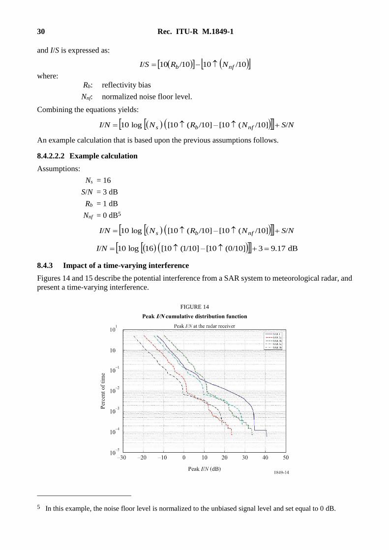
8.4.3 Impact of a time-varying interference

Figures 14 and 15 describe the potential interference from a SAR system to meteorological radar, and

present a time-varying interference.

FIGURE 14

Peak I/N cumulative distribution function

5 In this example, the noise floor level is normalized to the unbiased signal level and set equal to 0 dB.

Rec. ITU-R M.1849-1 31

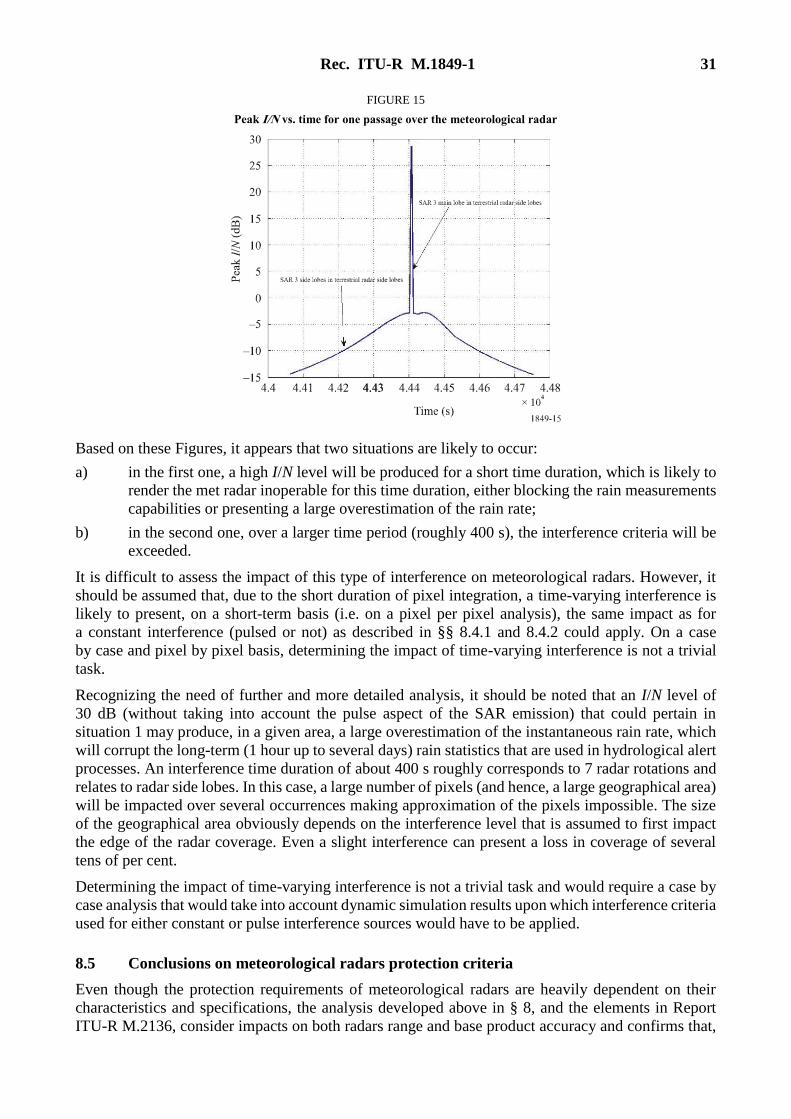
FIGURE 15

Peak I/N vs. time for one passage over the meteorological radar

Based on these Figures, it appears that two situations are likely to occur:

a) in the first one, a high I/N level will be produced for a short time duration, which is likely to

render the met radar inoperable for this time duration, either blocking the rain measurements

capabilities or presenting a large overestimation of the rain rate;

b) in the second one, over a larger time period (roughly 400 s), the interference criteria will be

exceeded.

It is difficult to assess the impact of this type of interference on meteorological radars. However, it

should be assumed that, due to the short duration of pixel integration, a time-varying interference is

likely to present, on a short-term basis (i.e. on a pixel per pixel analysis), the same impact as for

a constant interference (pulsed or not) as described in §§ 8.4.1 and 8.4.2 could apply. On a case

by case and pixel by pixel basis, determining the impact of time-varying interference is not a trivial

task.

Recognizing the need of further and more detailed analysis, it should be noted that an I/N level of

30 dB (without taking into account the pulse aspect of the SAR emission) that could pertain in

situation 1 may produce, in a given area, a large overestimation of the instantaneous rain rate, which

will corrupt the long-term (1 hour up to several days) rain statistics that are used in hydrological alert

processes. An interference time duration of about 400 s roughly corresponds to 7 radar rotations and

relates to radar side lobes. In this case, a large number of pixels (and hence, a large geographical area)

will be impacted over several occurrences making approximation of the pixels impossible. The size

of the geographical area obviously depends on the interference level that is assumed to first impact

the edge of the radar coverage. Even a slight interference can present a loss in coverage of several

tens of per cent.

Determining the impact of time-varying interference is not a trivial task and would require a case by

case analysis that would take into account dynamic simulation results upon which interference criteria

used for either constant or pulse interference sources would have to be applied.

8.5 Conclusions on meteorological radars protection criteria

Even though the protection requirements of meteorological radars are heavily dependent on their

characteristics and specifications, the analysis developed above in § 8, and the elements in Report

ITU-R M.2136, consider impacts on both radars range and base product accuracy and confirms that,

32 Rec. ITU-R M.1849-1

for constant interference, an I/N = −10 dB is relevant and hence should be used to ensure the

protection of meteorological radars. This criterion is consistent with existing

ITU-R Recommendations.

For pulsed interference analysis and tests have shown that, depending on characteristics of the

transmitter and victim system (primarily PRF and pulse width), a higher I/N relating to the peak power

of the pulsed interference. Pending further studies, one of the methods described in §§ 8.4.2 or 8.4.2.1

can be applied to represent an appropriate approximation.

At present, a generic formula for time-varying interference has not yet been developed. Depending

on whether the interference source is continuous or pulsed, is short term (impact on radar radials), or

if the interference is long term (overall volume scan), the analysis should be performed on a case-by-

case basis and from results of dynamic simulations, taking into account the relevant abovementioned

criteria for either constant or pulse like interference.

9 Impact of wind turbines

For accurate weather forecasting, weather radars are designed to look at a relatively narrow altitude

band. Due to the sensitivity of the radars, wind turbines, if deployed with line of site of a weather

radar facility, can block the onward propagation of the radar signals, cause reflectivity clutter returns,

and produce wake-turbulence-induced radar echoes. These interference mechanisms can result in

false radar estimates of precipitation accumulation, false tornadic and mesocycle signatures,

misidentification of thunderstorm features and incorrect storm cell identification. In addition, the

interference mechanisms can result in degraded radar performance and negatively impact forecast

and warning operations.

9.1 Masking

Any geographical feature or structure which lies between the radar and the target will cause

a shadowing or masking effect. It is possible that, depending on their size, wind turbines may cause

shadowing effects. Such shadowing effects may be expected to vary, depending on the turbine

dimensions, the type of transmitting radar and the aspect (height, blade angle, rotation rate, and

position relative to the radar of the turbine).

9.2 Clutter

Radar returns may be received from any radar-reflective surface. In certain geographical areas,

or under particular meteorological conditions, radar performance may be adversely affected by

unwanted returns, which may mask those of interest. Such unwanted returns are known as radar

clutter. For a weather forecaster, a wind turbine or turbines in the vicinity of weather radar can present

operational problems.

Ground clutter signals exhibit large reflectivity, near-zero Doppler shift, small spectrum width,

and are consistently localized. Compared to commonly occurring ground clutter (GC), interference

caused by wind turbines is a much more difficult challenge. Direct reflections will be received from

both the tower (stationary) and the blades (non-stationary). Like GC, the wind turbine clutter (WTC)

signal should still have a significantly large reflectivity, with a possible modulation due to blade

rotation causing a systematic variation in radar cross-section.

The Doppler shift will be affected by several factors, including the blade rotation speed and rotor

orientation with respect to the radar beam. Doppler velocities should be at a maximum when the rotor

is oriented 90° from the radar line-of-sight, and near zero when the rotor is facing either away or

toward the radar. Since the resolution volume of the radar will likely encompass the entire wind

turbine structure, it is expected that the spectrum width will be significantly enlarged. This is due to

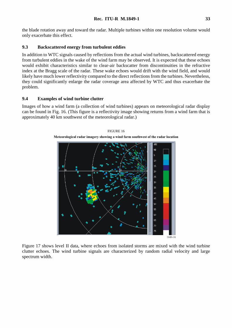
Rec. ITU-R M.1849-1 33

the blade rotation away and toward the radar. Multiple turbines within one resolution volume would

only exacerbate this effect.

9.3 Backscattered energy from turbulent eddies

In addition to WTC signals caused by reflections from the actual wind turbines, backscattered energy

from turbulent eddies in the wake of the wind farm may be observed. It is expected that these echoes

would exhibit characteristics similar to clear-air backscatter from discontinuities in the refractive

index at the Bragg scale of the radar. These wake echoes would drift with the wind field, and would

likely have much lower reflectivity compared to the direct reflections from the turbines. Nevertheless,

they could significantly enlarge the radar coverage area affected by WTC and thus exacerbate the

problem.

9.4 Examples of wind turbine clutter

Images of how a wind farm (a collection of wind turbines) appears on meteorological radar display

can be found in Fig. 16. (This figure is a reflectivity image showing returns from a wind farm that is

approximately 40 km southwest of the meteorological radar.)

FIGURE 16

Meteorological radar imagery showing a wind farm southwest of the radar location

Figure 17 shows level II data, where echoes from isolated storms are mixed with the wind turbine

clutter echoes. The wind turbine signals are characterized by random radial velocity and large

spectrum width.

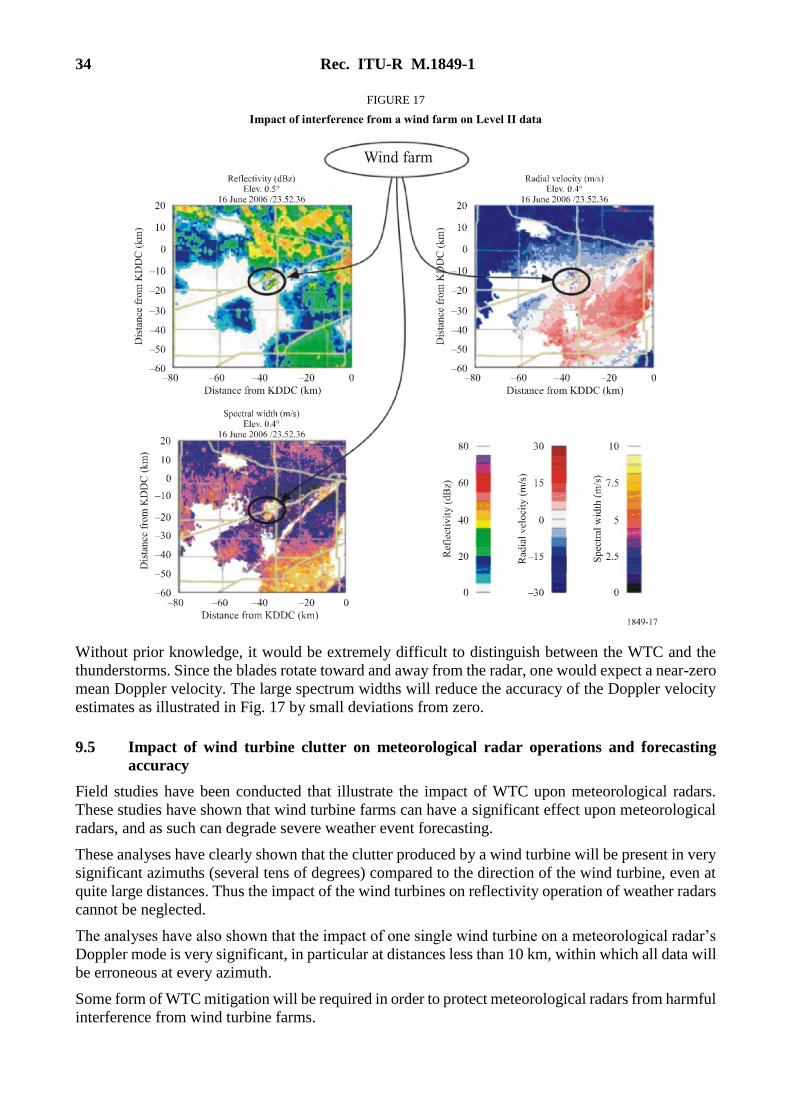
34 Rec. ITU-R M.1849-1

FIGURE 17

Impact of interference from a wind farm on Level II data

Without prior knowledge, it would be extremely difficult to distinguish between the WTC and the

thunderstorms. Since the blades rotate toward and away from the radar, one would expect a near-zero

mean Doppler velocity. The large spectrum widths will reduce the accuracy of the Doppler velocity

estimates as illustrated in Fig. 17 by small deviations from zero.

9.5 Impact of wind turbine clutter on meteorological radar operations and forecasting

accuracy

Field studies have been conducted that illustrate the impact of WTC upon meteorological radars.

These studies have shown that wind turbine farms can have a significant effect upon meteorological

radars, and as such can degrade severe weather event forecasting.

These analyses have clearly shown that the clutter produced by a wind turbine will be present in very

significant azimuths (several tens of degrees) compared to the direction of the wind turbine, even at

quite large distances. Thus the impact of the wind turbines on reflectivity operation of weather radars

cannot be neglected.

The analyses have also shown that the impact of one single wind turbine on a meteorological radar’s

Doppler mode is very significant, in particular at distances less than 10 km, within which all data will

be erroneous at every azimuth.

Some form of WTC mitigation will be required in order to protect meteorological radars from harmful

interference from wind turbine farms.

Rec. ITU-R M.1849-1 35

Before any final conclusions can be made regarding processing methods to mitigate WTC, additional

studies of WTC should be conducted in order to understand the full extent and the impact of WTC

on meteorological radars. Once this has been defined, methods to mitigate WTC may need to be

developed given the expected growth of wind-power based generation systems.

Pending the result of ongoing studies on mitigating WTC interference to meteorological radars,

the current solution to avoid or limit the impact of wind farms is to ensure separation distances

between the two systems. For example, some European countries are currently considering the

following recommendations:

a) that no wind turbine should be deployed at a range from radar antenna lower than:

– 5 km for radars operating in the frequency range 5 250-5 725 MHz;

– 10 km for radars operating in the frequency band 2 700-2 900 MHz;

b) that projects of wind parks should be submitted to an impact study when they concern ranges

lower than:

– 20 km for radars operating in the frequency range 5 250-5 725 MHz;

– 30 km for radars operating in the frequency band 2 700-2 900 MHz.

10 Previous tests of meteorological radar systems

Previous testing was conducted on meteorological radar with the objective of determining the radar’s

protection criteria. The procedure and data analysis methodology is defined in detail in Annex 1 of

Report ITU-R M.2136. The testing involved injecting an interference signal into the receiver at a

known level. The radar was allowed to perform a partial (1 or 2 antenna rotations) or full volume scan

without interference present. The radar would then be reset to perform the same partial or full volume

scan, with the interference signal injected into the receive path using an RF combiner. The base

products data for the non-interference and the interference partial or full volume scan was stored to

disk. The alternating non-interference and interference partial or full volume scans were conducted

at interference signal levels providing interference to noise ratios, I/N, ranging from +6 dB to –15 dB.

Data analysis was then conducted by making an interference-free range bin to interference-present

range bin comparison along each radial. From the regressed data, the I/N level at which the

interference causes the base products accuracy to fall outside acceptable limits could be determined.

The testing provided insight into potential testing improvements. The testing documented in Annex 1

of Report ITU-R M.2136 was performed with the radar collecting data from the atmosphere. The

assumption was the atmospheric conditions would not change significantly in the 3 to 5 minutes

required to perform the non-interference and interference partial or full volume scans. Data analysis

revealed this assumption was not always correct.

It is important to note that, across a broader range of meteorological radars, the sensitivity to

interference may vary as each individual radar’s tolerable interference level is dependent upon the

minimum signal-to-noise ratio of interest, estimate bias, and variance performance requirements.

More recent interference testing was performed to determine, for one type of meteorological radar

operating in the frequency range 5 250-5 725 MHz, interference sensitivity corresponding to different

interference signals (constant, CW or FM and pulsed) and confirmed the above analysis in § 8, as

well as previous testing related to meteorological radars operating in the frequency band 2 700-

2 900 MHz. A summary of these testing results is given in Annex 2 of Report ITU-R M.2136.

36 Rec. ITU-R M.1849-1

11 Future tests

Future testing methods should examine the use of a signal acquisition and regeneration system where

the radar IF or I and Q signals can be captured, digitized and stored to disk. The signals of a single

interference-free volume scan can be captured and digitized.

With use of arbitrary waveform generator(s) and an RF signal generator, the digitized received radar

signal can be recreated and injected into the radar receiver as many times as necessary to conduct the

testing, simulating return signals from the atmosphere. Such an approach may provide identical test

conditions for the non-interference and interference partial or full volume scans.

Testing with pulsed type interference and/or time-varying interference may need to be performed to

assess and confirm susceptibility of meteorological radars to this type of interference. This testing

should be conducted on both non-polarimetric (horizontally polarized) and polarimetric (horizontally

and vertically polarized) meteorological radars.

12 Propagation models

Previous sections discuss the need to minimize the amount of permissible interference received by

meteorological radars. However, it is also recognized that propagation models should be considered

when performing sharing studies and the more advanced propagation models, such as

Recommendations ITU-R P.452 and ITU-R P.526, provide the most accurate results for those studies.

These advanced propagation models require use of an exceedance value other than 0.0%. Additional

study is needed to better define the feasibility of using these advanced propagation models and how

the result should be properly applied in sharing studies.

13 Future trends

Major hardware upgrades to various administrations’ meteorological radar systems are in progress.

The next improvement will be polarimetric radar, which adds vertical polarization to the currently

used horizontal radar waves.

Additional techniques to further improve the performance of meteorological radars are also under

way. Foremost among these are various algorithms for resolving range/velocity ambiguities,

increasing data acquisition speed, reducing the effects of artefacts, decreasing clutter and efficient

processing of signals to provide meteorological estimates that are as accurate as possible. Other

endeavours include combined use of weather and profiling radars. A modest effort is devoted to

studies of lightning and its hazards, to determine whether its onset and termination might be

predictable.

Researchers will soon begin adapting phased array radar technology for use in weather surveillance

applications. The phased array will replace mechanically steered parabolic dish antennas with an

electronically steered array antenna. This change will enable more flexible scanning strategies and

more rapid updates of changing weather conditions. Early tests of the phased array radar system have

proved promising. Phased array technology will increase fundamental understanding of storm

evolution, in turn leading to improved computer models, more accurate forecasts and earlier

warnings. In addition, this technology has the potential to increase the average lead-time for tornado

warnings well beyond the current average of 13 min. No changes in transmitter output power or the

spectrum requirements of existing the system antennas to phased arrays. System enhancements are

more economically implemented via improvements to the receiver and signal processing subsystems.

Although phased array implementation is not anticipated within the next ten years, there is a

possibility that the phased array upgrade (if implemented) will not reuse the existing transmitter,

which will be replaced by distributed transmit/receive modules in the phased array.

Rec. ITU-R M.1849-1 37

A potential does exist for the deployment of CASA (Centre for collaborative adaptive sensing of the

atmosphere) based X-band weather radar systems within the 8 000 MHz to 12 000 MHz portion of

the frequency spectrum. The National Science Foundation established a new engineering research

centre for collaborative adaptive sensing of the atmosphere (CASA) in September 2003 to develop

small, low-cost radars for high-resolution sensing of the lower atmosphere. Meteorological conditions

in the lower troposphere are grossly under-sampled, inhibiting forecasts and model initialization in

the region where storms develop. The high spatial-density CASA radars will have the potential of

detecting evolving weather patterns in the region of the lower atmosphere that often lies below

existing operational Doppler radar coverage (i.e. the lowest three kilometres). CASA radars will be

placed on cell phone towers or other existing infrastructure with large data transmission capabilities.

Unlike the existing pre-programmed radar network, the collaborative CASA radars will communicate

with one another, and adapt their sensing strategies in direct response to the evolving weather and

changing end-user needs. These radar data can be incorporated into numerical weather prediction

models for more complete data initialization.

These future trends will need to be tracked and, as technologies evolve, will have an impact on any

future interference mitigation strategies and protection criteria definitions.

14 Summary

Ground-based meteorological radars operate and process signals differently than other radars, and

produce products much different than other radar types. These differences may affect how

interference analyses should be conducted, and how analysis results should be assessed.

Ground-based meteorological radars are specific, using different antenna movement strategies to

conduct a scan of the atmospheric volume around that radar, where a complete representation of the

atmospheric conditions is measured. In comparison, most other radar types track discrete targets and

are only concerned with returns for range cells that are associated with the targets. In meteorological

radar, all range cells in all radials are processed.

Annex 2

Characteristics of meteorological radars

1 Meteorological radars in the frequency band 2 700-2 900 MHz

The technical characteristics of representative weather radars that operate in the frequency band

2 700-2 900 MHz are depicted in Table 1. However, radar 1 can operate up to 3 000 MHz. These are

the primary weather radar systems which are used for flight planning activities. They are, on a

worldwide basis, often collocated at airports and provide accurate assessments of weather conditions

which are used to manage flight operations. These radars are in operation 24 h/day.

Radar 1 utilizes Doppler radar technology to observe the presence and calculate the speed and

direction of the motion of severe weather elements, such as tornadoes, hurricanes and violent

thunderstorms. Radar 1 also provides quantitative area precipitation measurements that play an

important role in hydrologic forecasting. The severe weather and motion detection capabilities offered

by this radar contribute towards an increase in the accuracy and timeliness of warning services.

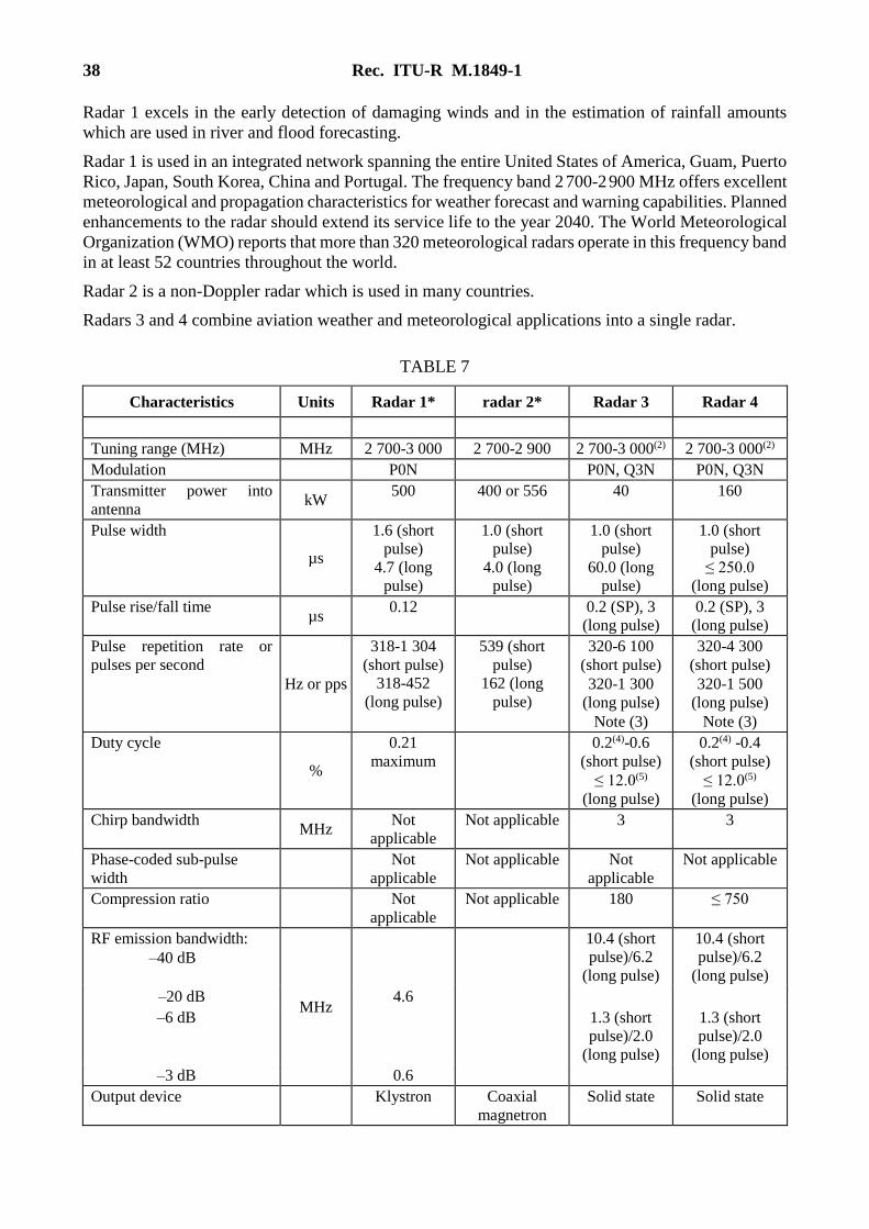
38 Rec. ITU-R M.1849-1

Radar 1 excels in the early detection of damaging winds and in the estimation of rainfall amounts

which are used in river and flood forecasting.

Radar 1 is used in an integrated network spanning the entire United States of America, Guam, Puerto

Rico, Japan, South Korea, China and Portugal. The frequency band 2 700-2 900 MHz offers excellent

meteorological and propagation characteristics for weather forecast and warning capabilities. Planned

enhancements to the radar should extend its service life to the year 2040. The World Meteorological

Organization (WMO) reports that more than 320 meteorological radars operate in this frequency band

in at least 52 countries throughout the world.

Radar 2 is a non-Doppler radar which is used in many countries.

Radars 3 and 4 combine aviation weather and meteorological applications into a single radar.

TABLE 7

Characteristics Units Radar 1* radar 2* Radar 3 Radar 4

Tuning range (MHz) MHz 2 700-3 000 2 700-2 900 2 700-3 000(2) 2 700-3 000(2)

Modulation P0N P0N, Q3N P0N, Q3N

Transmitter power into

antenna kW

500 400 or 556 40 160

Pulse width

µs

1.6 (short

pulse)

4.7 (long

pulse)

1.0 (short

pulse)

4.0 (long

pulse)

1.0 (short

pulse)

60.0 (long

pulse)

1.0 (short

pulse)

≤ 250.0

(long pulse)

Pulse rise/fall time µs

0.12 0.2 (SP), 3

(long pulse)

0.2 (SP), 3

(long pulse)

Pulse repetition rate or

pulses per second

Hz or pps

318-1 304

(short pulse)

318-452

(long pulse)

539 (short

pulse)

162 (long

pulse)

320-6 100

(short pulse)

320-1 300

(long pulse)

Note (3)

320-4 300

(short pulse)

320-1 500

(long pulse)

Note (3)

Duty cycle

%

0.21

maximum

0.2(4)-0.6

(short pulse)

≤ 12.0(5)

(long pulse)

0.2(4) -0.4

(short pulse)

≤ 12.0(5)

(long pulse)

Chirp bandwidth MHz

Not

applicable

Not applicable 3 3

Phase-coded sub-pulse

width

Not

applicable

Not applicable Not

applicable

Not applicable

Compression ratio

Not

applicable

Not applicable 180 ≤ 750

RF emission bandwidth:

–40 dB

MHz

10.4 (short

pulse)/6.2

(long pulse)

10.4 (short

pulse)/6.2

(long pulse)

–20 dB 4.6

–6 dB 1.3 (short

pulse)/2.0

(long pulse)

1.3 (short

pulse)/2.0

(long pulse)

–3 dB 0.6

Output device

Klystron Coaxial

magnetron

Solid state Solid state

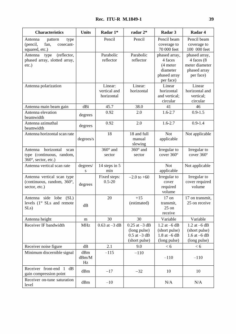
Rec. ITU-R M.1849-1 39

Characteristics Units Radar 1* radar 2* Radar 3 Radar 4

Antenna pattern type

(pencil, fan, cosecant-

squared, etc.)

Pencil Pencil Pencil beam

coverage to

70 000 feet

Pencil beam

coverage to

100 000 feet

Antenna type (reflector,

phased array, slotted array,

etc.)

Parabolic

reflector

Parabolic

reflector

phased array,

4 faces

(4 meter

diameter

phased array

per face)

phased array,

4 faces (8

meter diameter

phased array

per face)

Antenna polarization

Linear:

vertical and

horizontal

Linear:

horizontal

Linear

horizontal

and vertical;

circular

Linear

horizontal and

vertical;

circular

Antenna main beam gain dBi 45.7 38.0 41 46

Antenna elevation

beamwidth degrees

0.92 2.0 1.6-2.7 0.9-1.5

Antenna azimuthal

beamwidth degrees

0.92 2.0 1.6-2.7 0.9-1.4

Antenna horizontal scan rate

degrees/s

18 18 and full

manual

slewing

Not

applicable

Not applicable

Antenna horizontal scan

type (continuous, random,

360°, sector, etc.)

360° and

sector

360° and

sector

Irregular to

cover 360o

Irregular to

cover 360o

Antenna vertical scan rate degrees/

s

14 steps in 5

min

Not

applicable

Not applicable

Antenna vertical scan type

(continuous, random, 360°,

sector, etc.) degrees

Fixed steps:

0.5-20 2.0 to +60 Irregular to

cover

required

volume

Irregular to

cover required

volume

Antenna side lobe (SL)

levels (1st SLs and remote

SLs) dB

20 +15

(estimated)

17 on

transmit,

25 on

receive

17 on transmit,

25 on receive

Antenna height m 30 30 Variable Variable

Receiver IF bandwidth MHz 0.63 at –3 dB 0.25 at –3 dB

(long pulse)

0.5 at –3 dB

(short pulse)

1.2 at –6 dB

(short pulse)

1.8 at –6 dB

(long pulse)

1.2 at –6 dB

(short pulse)

1.6 at –6 dB

(long pulse)

Receiver noise figure dB 2.1 9.0 < 6 < 6

Minimum discernible signal dBm

dBm/M

Hz

–115 110

–110

–110

Receiver front-end 1 dB

gain compression point dBm –17 32 10 10

Receiver on-tune saturation

level dBm –10 N/A N/A

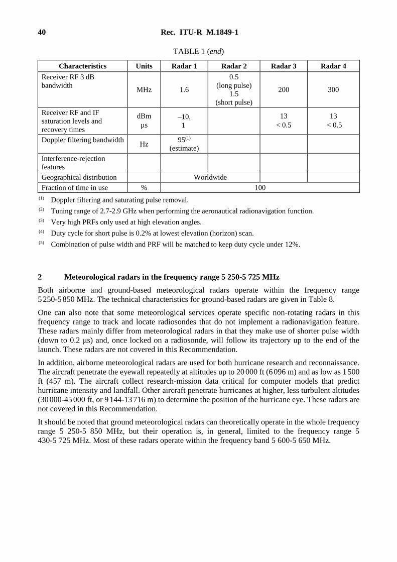
40 Rec. ITU-R M.1849-1

TABLE 1 (end)

Characteristics Units Radar 1 Radar 2 Radar 3 Radar 4

Receiver RF 3 dB

bandwidth MHz 1.6

0.5

(long pulse)

1.5

(short pulse)

200 300

Receiver RF and IF

saturation levels and

recovery times

dBm

µs –10,

1 13

< 0.5

13

< 0.5

Doppler filtering bandwidth Hz

95(1)

(estimate)

Interference-rejection

features

Geographical distribution Worldwide

Fraction of time in use % 100

(1) Doppler filtering and saturating pulse removal.

(2) Tuning range of 2.7-2.9 GHz when performing the aeronautical radionavigation function.

(3) Very high PRFs only used at high elevation angles.

(4) Duty cycle for short pulse is 0.2% at lowest elevation (horizon) scan.

(5) Combination of pulse width and PRF will be matched to keep duty cycle under 12%.

2 Meteorological radars in the frequency range 5 250-5 725 MHz

Both airborne and ground-based meteorological radars operate within the frequency range

5 250-5 850 MHz. The technical characteristics for ground-based radars are given in Table 8.

One can also note that some meteorological services operate specific non-rotating radars in this

frequency range to track and locate radiosondes that do not implement a radionavigation feature.

These radars mainly differ from meteorological radars in that they make use of shorter pulse width

(down to 0.2 μs) and, once locked on a radiosonde, will follow its trajectory up to the end of the

launch. These radars are not covered in this Recommendation.

In addition, airborne meteorological radars are used for both hurricane research and reconnaissance.

The aircraft penetrate the eyewall repeatedly at altitudes up to 20 000 ft (6 096 m) and as low as 1 500

ft (457 m). The aircraft collect research-mission data critical for computer models that predict

hurricane intensity and landfall. Other aircraft penetrate hurricanes at higher, less turbulent altitudes

(30 000-45 000 ft, or 9 144-13 716 m) to determine the position of the hurricane eye. These radars are

not covered in this Recommendation.

It should be noted that ground meteorological radars can theoretically operate in the whole frequency

range 5 250-5 850 MHz, but their operation is, in general, limited to the frequency range 5

430-5 725 MHz. Most of these radars operate within the frequency band 5 600-5 650 MHz.

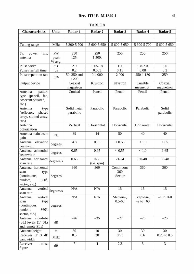
Rec. ITU-R M.1849-1 41

TABLE 8

Characteristics Units Radar 1 Radar 2 Radar 3 Radar 4 Radar 5

Tuning range MHz 5 300-5 700 5 600-5 650 5 600-5 650 5 300-5 700 5 600-5 650

Tx power into

antenna

kW

peak

W avg.

250

125.

250

1 500.

250 250 250

Pulse width µs 2.0 0.05-18 1.1 0.8-2.0 3.0

Pulse rise/fall time µs 0.2 0.005 0.11 0.08 0.3

Pulse repetition rate pps

50, 250 and

1 200

0-4 000 2 000 250-1 180 259

Output device

Coaxial

magnetron

Klystron Klystron Tunable

magnetron

Coaxial

magnetron

Antenna pattern

type (pencil, fan,

cosecant-squared,

etc.)

Conical Pencil Pencil Pencil Pencil

Antenna type

(reflector, phased

array, slotted array,

etc.)

Solid metal

parabolic

Parabolic Parabolic Parabolic Solid

parabolic

Antenna

polarization

Vertical Horizontal Horizontal Horizontal Horizontal

Antenna main beam

gain dBi

39 44 50 40 40

Antenna elevation

beamwidth degrees

4.8 0.95 < 0.55 < 1.0 1.65

Antenna azimuthal

beamwidth degrees

0.65 0.95 < 0.55 < 1.0 1.65

Antenna horizontal

scan rate degrees/s

0.65 0-36

(0-6 rpm)

21-24 30-48 30-48

Antenna horizontal

scan type

(continuous,

random, 360⁰, sector, etc.)

degrees

360 360 Continuous

360

Sector

360 360

Antenna vertical

scan rate degrees/s

N/A N/A 15 15 15

Antenna vertical

scan type

(continuous,

random, 360⁰, sector, etc.)

degrees

N/A N/A Stepwise,

0.5-60

Stepwise,

–2 to +60

–1 to +60

Antenna side-lobe

(SL) levels (1st SLs

and remote SLs)

dB

–26 –35 –27 –25 –25

Antenna height m 30 10 30 30 30

Receiver IF 3 dB

bandwidth MHz

0.5 20 0.91 0.6 0.25 to 0.5

Receiver noise

figure dB

7 4 2.3 3 3

.

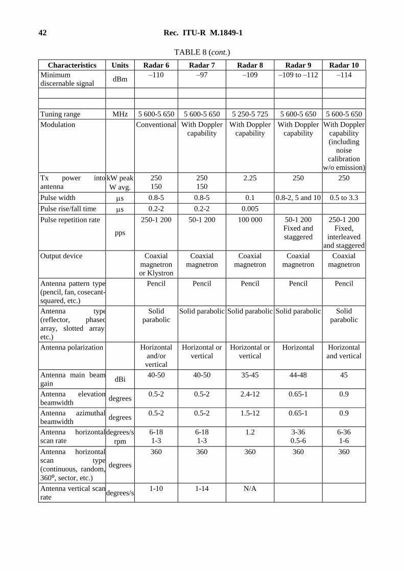
42 Rec. ITU-R M.1849-1

TABLE 8 (cont.)

Characteristics Units Radar 6 Radar 7 Radar 8 Radar 9 Radar 10

Minimum

discernable signal dBm

–110 –97 –109 –109 to –112 –114

Tuning range MHz 5 600-5 650 5 600-5 650 5 250-5 725 5 600-5 650 5 600-5 650

Modulation

Conventional With Doppler

capability

With Doppler

capability

With Doppler

capability

With Doppler

capability

(including

noise

calibration

w/o emission)

Tx power into

antenna

kW peak

W avg.

250

150

250

150

2.25 250 250

Pulse width s 0.8-5 0.8-5 0.1 0.8-2, 5 and 10 0.5 to 3.3

Pulse rise/fall time s 0.2-2 0.2-2 0.005

Pulse repetition rate

pps

250-1 200 50-1 200 100 000 50-1 200

Fixed and

staggered

250-1 200

Fixed,

interleaved

and staggered

Output device

Coaxial

magnetron

or Klystron

Coaxial

magnetron

Coaxial

magnetron

Coaxial

magnetron

Coaxial

magnetron

Antenna pattern type

(pencil, fan, cosecant-

squared, etc.)

Pencil Pencil Pencil Pencil Pencil

Antenna type

(reflector, phased

array, slotted array,

etc.)

Solid

parabolic

Solid parabolic Solid parabolic Solid parabolic Solid

parabolic

Antenna polarization

Horizontal

and/or

vertical

Horizontal or

vertical

Horizontal or

vertical

Horizontal Horizontal

and vertical

Antenna main beam

gain dBi

40-50 40-50 35-45 44-48 45

Antenna elevation

beamwidth degrees

0.5-2 0.5-2 2.4-12 0.65-1 0.9

Antenna azimuthal

beamwidth degrees

0.5-2 0.5-2 1.5-12 0.65-1 0.9

Antenna horizontal

scan rate

degrees/s

rpm

6-18

1-3

6-18

1-3

1.2 3-36

0.5-6

6-36

1-6

Antenna horizontal

scan type

(continuous, random,

360⁰, sector, etc.)

degrees

360 360 360 360 360

Antenna vertical scan

rate degrees/s

1-10 1-14 N/A

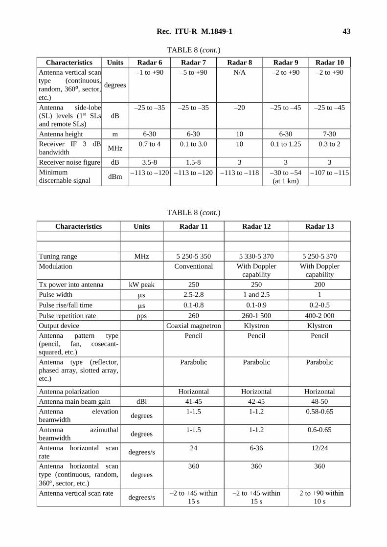
Rec. ITU-R M.1849-1 43

TABLE 8 (cont.)

Characteristics Units Radar 6 Radar 7 Radar 8 Radar 9 Radar 10

Antenna vertical scan

type (continuous,

random, 360⁰, sector,

etc.)

degrees

–1 to +90 –5 to +90 N/A –2 to +90 –2 to +90

Antenna side-lobe

(SL) levels (1st SLs

and remote SLs)

dB

–25 to –35 –25 to –35 –20 –25 to –45 –25 to –45

Antenna height m 6-30 6-30 10 6-30 7-30

Receiver IF 3 dB

bandwidth MHz

0.7 to 4 0.1 to 3.0 10 0.1 to 1.25 0.3 to 2

Receiver noise figure dB 3.5-8 1.5-8 3 3 3

Minimum

discernable signal dBm

113 to 120 113 to 120 113 to 118 30 to 54

(at 1 km)

107 to 115

TABLE 8 (cont.)

Characteristics Units Radar 11 Radar 12 Radar 13

Tuning range MHz 5 250-5 350 5 330-5 370 5 250-5 370

Modulation

Conventional With Doppler

capability

With Doppler

capability

Tx power into antenna kW peak 250 250 200

Pulse width s 2.5-2.8 1 and 2.5 1

Pulse rise/fall time s 0.1-0.8 0.1-0.9 0.2-0.5

Pulse repetition rate pps 260 260-1 500 400-2 000

Output device Coaxial magnetron Klystron Klystron

Antenna pattern type

(pencil, fan, cosecant-

squared, etc.)

Pencil Pencil Pencil

Antenna type (reflector,

phased array, slotted array,

etc.)

Parabolic Parabolic Parabolic

Antenna polarization Horizontal Horizontal Horizontal

Antenna main beam gain dBi 41-45 42-45 48-50

Antenna elevation

beamwidth degrees

1-1.5 1-1.2 0.58-0.65

Antenna azimuthal

beamwidth degrees

1-1.5 1-1.2 0.6-0.65

Antenna horizontal scan

rate degrees/s

24 6-36 12/24

Antenna horizontal scan

type (continuous, random,

360, sector, etc.)

degrees

360 360 360

Antenna vertical scan rate degrees/s

–2 to +45 within

15 s

–2 to +45 within

15 s

−2 to +90 within

10 s

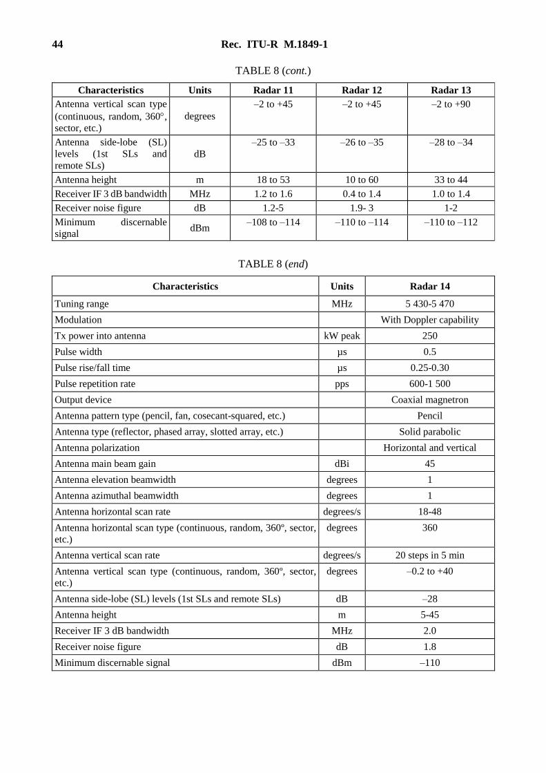
44 Rec. ITU-R M.1849-1

TABLE 8 (cont.)

Characteristics Units Radar 11 Radar 12 Radar 13

Antenna vertical scan type

(continuous, random, 360,

sector, etc.)

degrees

–2 to +45 –2 to +45 –2 to +90

Antenna side-lobe (SL)

levels (1st SLs and

remote SLs)

dB

–25 to –33 –26 to –35 –28 to –34

Antenna height m 18 to 53 10 to 60 33 to 44

Receiver IF 3 dB bandwidth MHz 1.2 to 1.6 0.4 to 1.4 1.0 to 1.4

Receiver noise figure dB 1.2-5 1.9- 3 1-2

Minimum discernable

signal dBm

–108 to –114 –110 to –114 –110 to –112

TABLE 8 (end)

Characteristics Units Radar 14

Tuning range MHz 5 430-5 470

Modulation With Doppler capability

Tx power into antenna kW peak 250

Pulse width µs 0.5

Pulse rise/fall time µs 0.25-0.30

Pulse repetition rate pps 600-1 500

Output device Coaxial magnetron

Antenna pattern type (pencil, fan, cosecant-squared, etc.) Pencil

Antenna type (reflector, phased array, slotted array, etc.) Solid parabolic

Antenna polarization Horizontal and vertical

Antenna main beam gain dBi 45

Antenna elevation beamwidth degrees 1

Antenna azimuthal beamwidth degrees 1

Antenna horizontal scan rate degrees/s 18-48

Antenna horizontal scan type (continuous, random, 360º, sector,

etc.)

degrees 360

Antenna vertical scan rate degrees/s 20 steps in 5 min

Antenna vertical scan type (continuous, random, 360º, sector,

etc.)

degrees –0.2 to +40

Antenna side-lobe (SL) levels (1st SLs and remote SLs) dB –28

Antenna height m 5-45

Receiver IF 3 dB bandwidth MHz 2.0

Receiver noise figure dB 1.8

Minimum discernable signal dBm –110

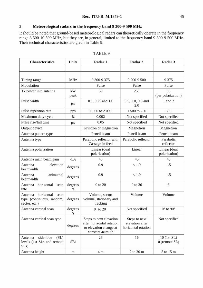
Rec. ITU-R M.1849-1 45

3 Meteorological radars in the frequency band 9 300-9 500 MHz

It should be noted that ground-based meteorological radars can theoretically operate in the frequency

range 8 500-10 500 MHz, but they are, in general, limited to the frequency band 9 300-9 500 MHz.

Their technical characteristics are given in Table 9.

TABLE 9

Characteristics Units Radar 1 Radar 2 Radar 3

Tuning range MHz 9 300-9 375 9 200-9 500 9 375

Modulation Pulse Pulse Pulse

Tx power into antenna kW

peak

50 250 35

(per polarization)

Pulse width s

0.1, 0.25 and 1.0 0.5, 1.0, 0.8 and

2.0

1 and 2

Pulse repetition rate pps 1 000 to 2 000 1 500 to 250 500

Maximum duty cycle % 0.002 Not specified Not specified

Pulse rise/fall time s 0.05 Not specified Not specified

Output device Klystron or magnetron Magnetron Magnetron

Antenna pattern type Pencil beam Pencil beam Pencil beam

Antenna type

Parabolic reflector with

Cassegrain feed

Parabolic reflector Parabolic

reflector

Antenna polarization

Linear (dual

polarization)

Linear Linear (dual

polarization)

Antenna main beam gain dBi 46 45 40

Antenna elevation

beamwidth degrees

0.9 < 1.0 1.5

Antenna azimuthal

beamwidth degrees

0.9 < 1.0 1.5

Antenna horizontal scan rate

degrees/s

0 to 20 0 to 36 6

Antenna horizontal scan

type (continuous, random, sector, etc.)

degrees

Volume, sector

volume, stationary and tracking

Volume Volume

Antenna vertical scan degrees

/s 0° to 20 Not specified 0° to 90°

Antenna vertical scan type

degrees

Steps to next elevation

after horizontal rotation

or elevation change at

constant azimuth

Steps to next

elevation after horizontal rotation

Not specified

Antenna side-lobe (SL)

levels (1st SLs and remote SLs)

dBi

26 16 10 (1st SL)

0 (remote SL)

Antenna height m 4 m 2 to 30 m 5 to 15 m

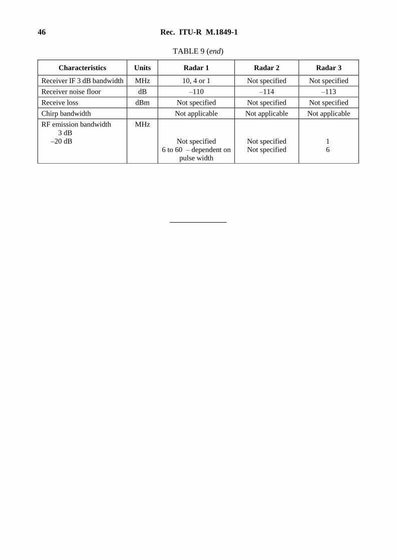
46 Rec. ITU-R M.1849-1

TABLE 9 (end)

Characteristics Units Radar 1 Radar 2 Radar 3

Receiver IF 3 dB bandwidth MHz 10, 4 or 1 Not specified Not specified

Receiver noise floor dB –110 –114 –113

Receive loss dBm Not specified Not specified Not specified

Chirp bandwidth Not applicable Not applicable Not applicable

RF emission bandwidth

3 dB

–20 dB

MHz

Not specified

6 to 60 – dependent on pulse width

Not specified Not specified

1 6