Page 1
-1
Aerodynamic Study of a Small, Ducted VTOL Aerial Vehicle
by
Kyrilian Dyer
S.B. Mechanical Engineering, MIT 2000
Submitted to the Department of Aeronautics and Astronautics in Partial Fulfillment of theRequirements for the Degree of MASTER OF SCIENCE in
AERONAUTICS & ASTRONAUTICS
at the
MASSACHUSETTS INSTITUTE OF TECHNOLOGY
June 2002
© 2002 Kyrilian Dyer. All rights reserved.
The author hereby grants to MIT permission to reproduce and distribute publicly paperand electronic copies of this thesis document in whole or in part.
Signature of Author:
Depart-dnht of Aeronatis & Astronautics
May 2002
Certified by:
Sean George
Charles Stark Draper Laboratory
(' Thesis Sunevisor
Certified by:
Professor John Deyst
Professor of Aeronautics & Astronautics
, J / . I p . Yhesis Advisor
Accepted by:
MASSACHUSETTS STITUTEOF TECHNOLOGY
AUG 1 3 002
LIBRARIES
Wallace E. Vander Velde
Professor of Aeronautics and Astronautics
Chair, Committee on Graduate Students
ARO
A A
Page 2
[ THIS PAGE INTENTIONALLY LEFT BLANK ]
2
Page 3
Aerodynamic Study of a Small, Ducted VTOL Aerial Vehicle
by
Kyrilian G. Dyer
Submitted to the Department of Aeronautics and Astronautics on May 10, 2002 in partial
fulfillment of the requirements for the Degree of Master of Science in
Aeronautics and Astronautics.
Abstract
The Perching Unmanned Aerial Vehicle (PUAV) is a 9-inch diameter ducted vertical takeoff and
landing reconnaissance vehicle with the capability of fast-forward cruise flight. Currently in the
development stage, the program is envisaged to yield a man-portable craft that a foot soldier can
use to provide over-the-hill observation. Several prototypes have been constructed and tested,
with mixed results. Concerns regarding duct aerodynamics led to the proposal for further
aerodynamic study to investigate effects of inlet lip radius and surface area, diffuser area ratio,
blade tip clearance and rotor position on thrust, power and efficiency. This report covers the
theory of rotorcraft and ducted propeller aerodynamics, and outlines the tests performed and
results obtained. It also presents specifications of the test vehicle and methods that can be used in
future ducted aircraft studies.
Large angle diffusers tested showed reduced thrust and efficiency and increased power compared
to smaller diffusers, contrary to theory. Reverse flow within the core appears to disrupt uniform
exit flow and yields a conically divergent turbulent wake. Results of this study will be used in the
redesign of a duct core fairing, which will act to control the airflow and reduce the tendency for
reverse flow at the center where blade thrust is absent. Future studies will also consider twisted,
cambered and tapered rotor blades in an effort to better address spanwise thrust distribution and
optimized airflow.
The test apparatus and methods developed for this report, in addition to results of initial testing,
will be instrumental to further development of small ducted UAVs. Findings and methods are not
limited to exact duplicates of PUAV-like aircraft, but can be used in a wide range of applications
including lift and thrust-producing ducts.
Technical Supervisor: Mr. Sean GeorgeTitle: Charles Stark Draper Laboratory
Thesis Advisor: Professor John DeystTitle: Professor, Aeronautics and Astronautics
3
Page 4
AcknowledgmentsJune, 2002
This thesis was prepared at The Charles Stark Draper Laboratory, Inc., under Internal
Company Sponsored Research Project 3019, Navigating Under the Canopy.
Publication of this thesis does not constitute approval by Draper of the findings or
conclusions contained herein. It is published for the exchange and stimulation of ideas.
j C (Author's signature)
I would like to thank all those who have made this fun little project move forward. I am
grateful to Sean George for devoting his time and wisdom to this project. Thanks to
Jamie Anderson for giving me direction and to John Plump and Neil Gupta for
conceiving the project and giving it life. I have enjoyed the friendship and enthusiasm of
Neil and Paul Eremenko. Thanks also to Tim Barrows and Professor John Deyst for their
input and wisdom. Without the help of Kailas Narendran and Dave Weagle, I wouldn't
have had the hardware to go forward. I've enjoyed sharing a relaxed and friendly office,
thanks to Dave, Kara, Carissa, Jeb and Matt. Of course, thanks to all my friends for their
support and understanding. Finally, thank you Mom and Dad, for your quiet
encouragement and gentle guidance.
4
Page 5
Table of Contents
Chapter 1: Introduction....................................................................................................... 9
Chapter 2: Background and H istory ................................................................................... 13
2.1 D esign Requirem ents .................................................................................................. 13
2.2 Survey of Sim ilar Aircraft............................................................................................ 15
2.2.1 H istory of V ertical Takeoff A ircraft ................................................................... 15
2.2.2 Current V ertical Takeoff U AV s.......................................................................... 16
2.3 PU A V D evelopm ent Evolution................................................................................... 20
2.3.1 Prelim inary D esign .............................................................................................. 22
2.3.2 A lpha Prototype Design ........................................................................................ 23
2.3.3 Beta Prototype Design ......................................................................................... 27
Chapter 3: Theoretical Perform ance................................................................................... 31
3.1 Rotorcraft A erodynam ics ............................................................................................ 31
3.1.1 M om entum Theory .............................................................................................. 31
3.1.2 Blade Elem ent Theory ......................................................................................... 39
3.1.3 Coaxial M om entum Theory .................................................................................. 44
3.1.4 D ucted Rotor Perform ance................................................................................... 46
3.2 Other Inlet and D iffuser Effects ................................................................................... 49
3.2.1 Inlet Thrust Augm entation ................................................................................... 50
3.2.2 Inlet Losses ........................................................................................ . ...... 54
3.2.3 Duct and D iffuser Losses ..................................................................................... 57
3.3 PU A V Num erical M odel......................................................................................... .... 57
Chapter 4: Experimental Test Apparatus.......................................................................... 61
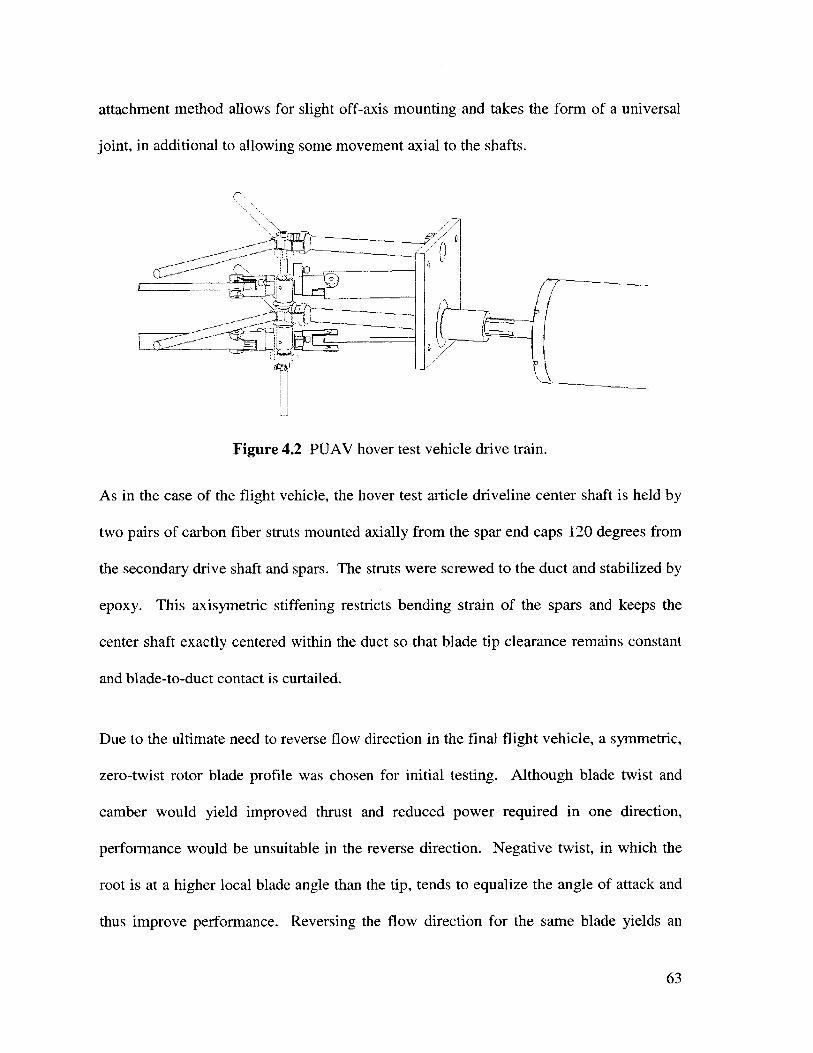
4.1 D rive Train ................................................................................ . -- .. . ---............. 61
4.1.1 Driveline .................................................................................................................. 61
4.1.2 Test M otor................................................................................................................ 67
4.2 D uct Construction ....................................................................................................... 69
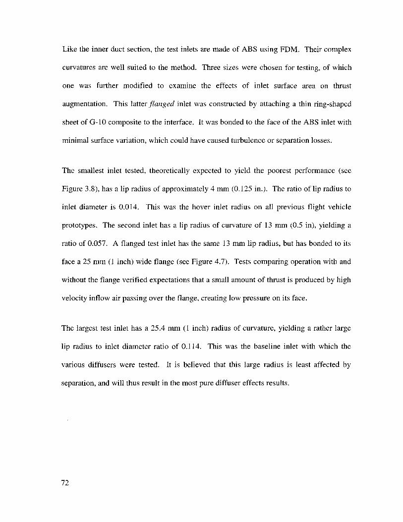
4.2.1 Inlets......................................................................................... . -------------.......... 71
4.2.2 Exit D iffusers ............................................................................. .. .. ..... 73
4.3 D ata A cquisition............................................................................... ... .......... 75
4.3.1 H ardw are...................................................................................--------------------.......... 75
4.3.2 D ata A cquisition Software ................................................................................... 78
5
Page 6
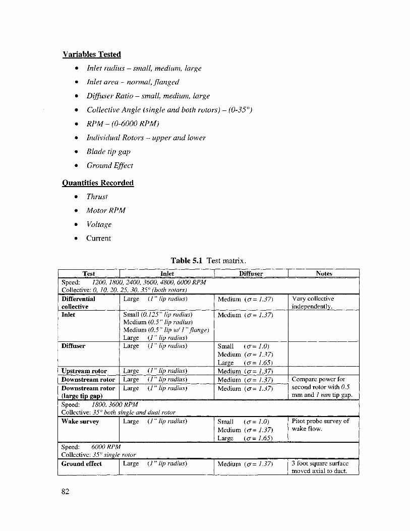
Chapter 5: Data Collection and Analysis ........................................................................... 81
5.1 Test M atrix Design .......................................................................................................... 81
5.2 Calibration....................................................................................................................... 83
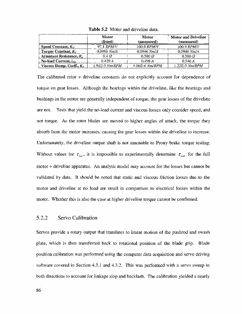
5.2.1 M otor Calibration................................................................................................ 83
5.2.2 Servo Calibration .................................................................................................. 86
5.2.3 Differential Collective......................................................................................... 87
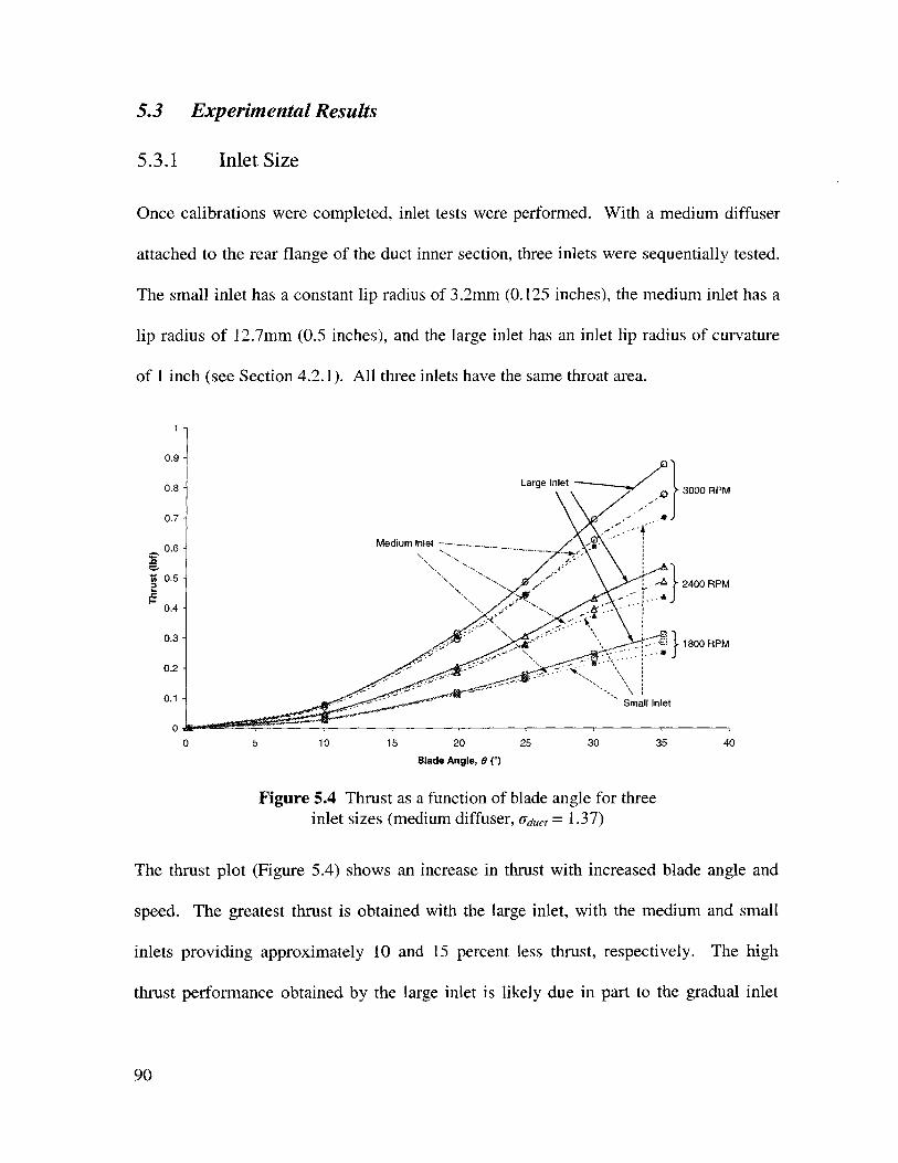
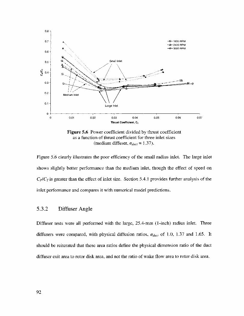
5.3 Experimental Results................................................................................................... 90
5.3.1 Inlet Size .................................................................................................................. 90
5.3.2 Diffuser Angle..................................................................................................... 92
5.3.3 Num ber of Rotors................................................................................................ 95
5.3.4 Blade Tip clearance.............................................................................................. 97
5.3.5 Ground Effect........................................................................................................... 98
5.3.6 W ake Survey ............................................................................................................ 99
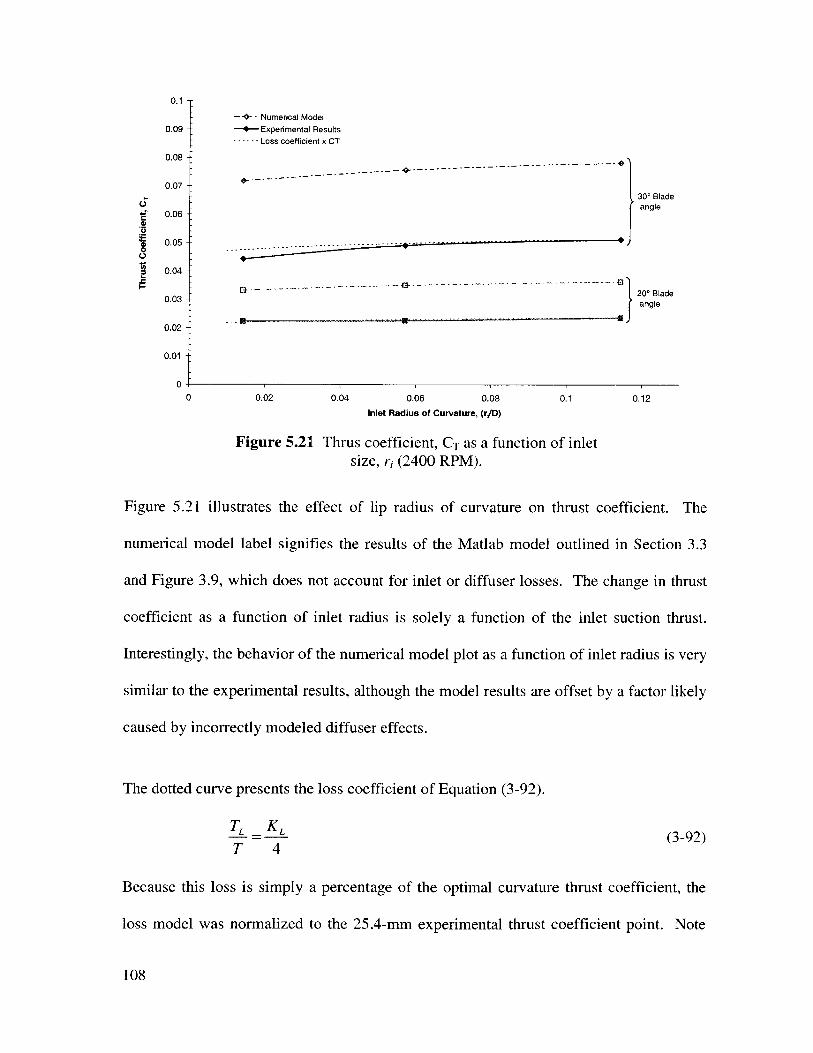
5.4 Results Analysis and M odel Comparison ..................................................................... 105
5.4.1 Inlet Size ................................................................................................................ 105
5.4.2 Diffusion Ratio....................................................................................................... 111
Chapter 6: Conclusion ............................................................................................................ 117
References ................................................................................................................................ 119
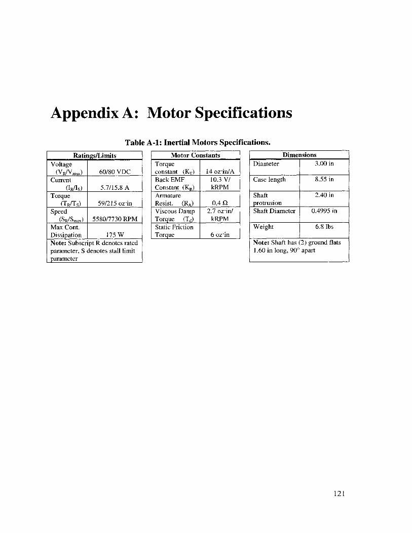
Appendix A : M otor Specifications .......................................................................................... 121
List of Figures
Figure 1.1 The PUAV Alpha II prototype ................................................................................ 10
Figure 1.2 Takeoff (a) and landing (b) of the PUAV ............................... 10
Figure 2.1 MAV deployment from "parent" vehicle system (Gupta [4])................................. 14
Figure 2.2 Sikorsky Cypher.......................................................................................................... 17
Figure 2.3 Allied Aerospace Industries iSTAR (LADF) (a) without and (b) with wings. ........ 19
Figure 2.4 Preliminary PUAV design architecture (from Gupta [4]). .................... 22
Figure 2.5 Alpha I prototype..................................................................................................... 24
Figure 2.6 Alpha I prototype thrust test apparatus (from Gupta [4]).................... 25
Figure 2.7 Alpha II prototype, with redesigned forebody.......................................................... 26
Figure 2.8 Alpha II thrust test apparatus................................................................................... 27
Figure 2.9 Beta prototype. ............................................................................................................ 28
6
Page 7
Figure 3.1 Helicopter rotor control volume............................................................................. 32
Figure 3.2 Theoretical PUAV figure of merit for different diffusion ratios.............................. 38
Figure 3.3 Inflow and force components of a blade element. From above (a) and spanwise (b).40
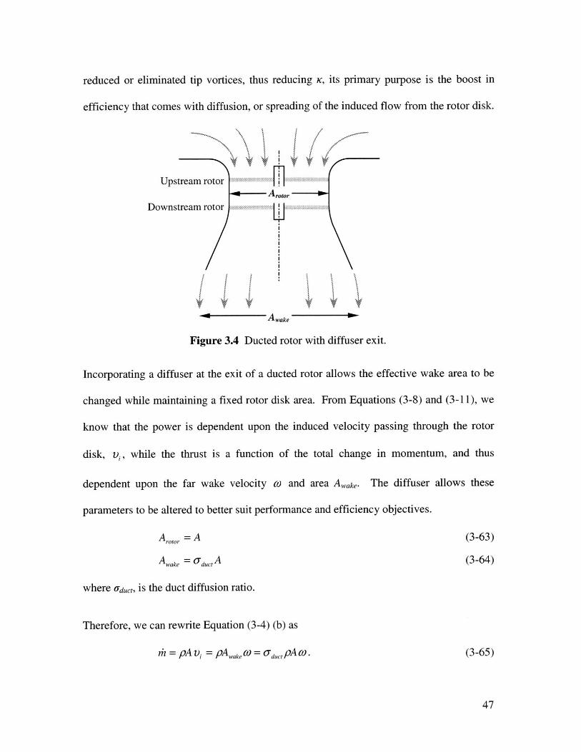
Figure 3.4 Ducted rotor with diffuser exit. ............................................................................... 47
Figure 3.5 Streamlines (a), and pressure distribution (b) over the inlet.................................... 50
Figure 3.6 Inlet surface area geometry. ................................................................................... 52
Figure 3.7 V ena contracta............................................................................................ ..... 55
Figure 3.8 Thrust losses due to sharp inlet curvature. .............................................................. 56
Figure 3.9 Com putational Flowchart......................................................................................... 59
Figure 4.1 Schematic diagram of PUAV hover test vehicle drive train. .................. 62
Figure 4.2 PUAV hover test vehicle drive train. ..................................................................... 63
Figure 4.3 NHP Tail rotor blade sectional lift and drag coefficient. ........................................ 64
Figure 4.4 Rotor collective control diagram..............................................................................66
Figure 4.5 RPM vs. torque available and required. ...................................................................... 68
Figure 4.6 Duct/drive train interface........................................................................................71
Figure 4.7 Section diagrams of four test inlets. ........................................................................ 73
Figure 4.8 Diagram of three test diffusers. ................................................................................... 74
Figure 4.9 Construction of a diffuser....................................................................................... 75
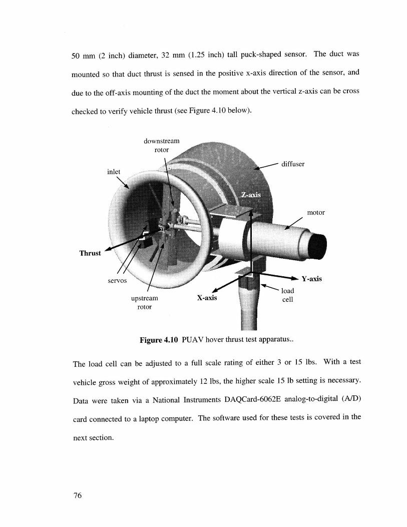
Figure 4.10 PUAV hover thrust test apparatus......................................................................... 76
Figure 4.11 Mechanical (a), and electrical (b) test apparatus layout........................................77
Figure 5.1 Motor test stand and Prony brake........................................................................... 84
Figure 5.2 Servo calibration curves ......................................................................................... 87
Figure 5.3 Differential Collective calibration test results......................................................... 89
Figure 5.4 Thrust as a function of blade angle for three inlet sizes (medium diffuser, aduc, = 1.37)......... 9...............................................90
Figure 5.5 Power as a function of blade angle for three inlet sizes (medium diffuser, oedc = 1.37)
................................................................................................. 91
Figure 5.6 Power coefficient divided by thrust coefficient as a function of thrust coefficient for
three inlet sizes (m edium diffuser, u educ = 1.37)...................................................................... 92
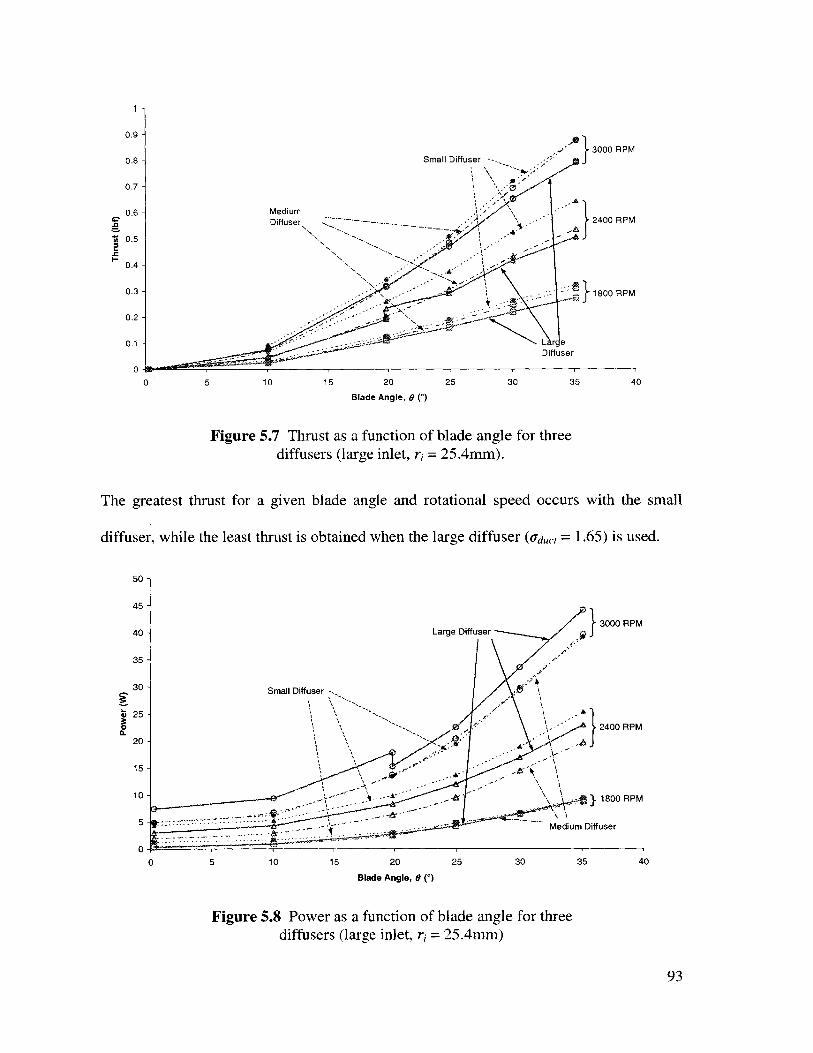
Figure 5.7 Thrust as a function of blade angle for three diffusers (large inlet, ri = 25.4mm).......93
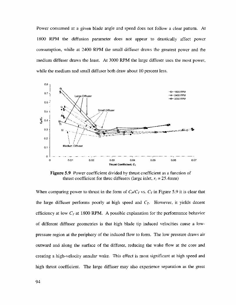
Figure 5.8 Power as a function of blade angle for three diffusers (large inlet, r, = 25.4mm)....... 93
Figure 5.9 Power coefficient divided by thrust coefficient as a function of thrust coefficient for
three diffusers (large inlet, r = 25.4mm)........................................................................... 94
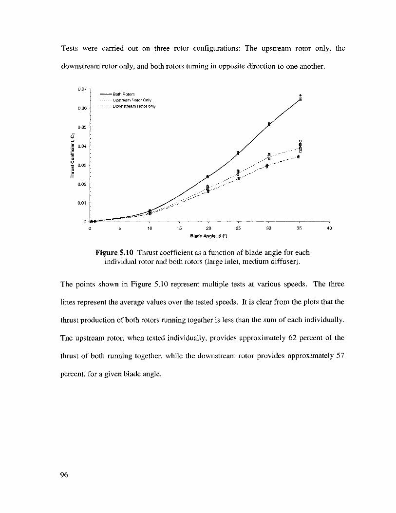
Figure 5.10 Thrust coefficient as a function of blade angle for each individual rotor and both
rotors (large inlet, medium diffuser)....................................................................... ... .. 96
7
Page 8
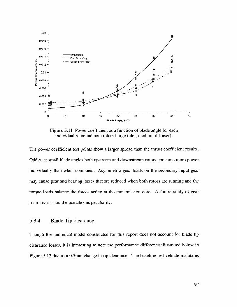
Figure 5.11 Power coefficient as a function of blade angle for each individual rotor and bothrotors (large inlet, medium diffuser)...................................................................................97
Figure 5.12 Power coefficient as a function of thrust coefficient for a 0.5 and 1 mm blade tip gap(large inlet, m edium diffuser)................................................................................................. 98
Figure 5.13 CP/CT as a function of height................................................................................. 99
Figure 5.14 Wake flow for (a) small diffuser (aqdc, = 1.0), (b) medium diffuser (qd, = 1.37), and(c) large diffuser (qd,, = 1.65) with single rotor at 3000 RPM. ........................................... 100
Figure 5.15 Wake survey comparison of single rotor with cone-shaped fairing and dual rotorw ithout a fairing. .................................................................................................................. 10 1
Figure 5.16 Thrust coefficient as a function of rotor RPM with and without a cone-shaped fairing(single rotor, 350 fixed). ................................................................................................ . 102
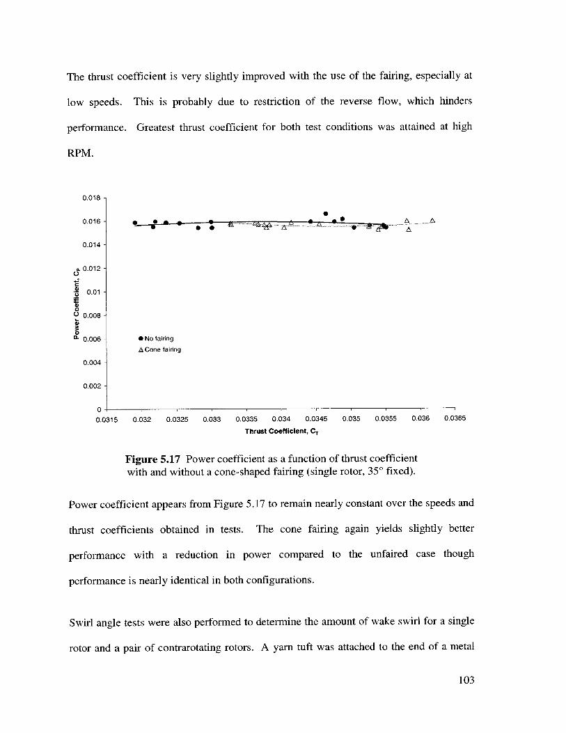
Figure 5.17 Power coefficient as a function of thrust coefficient with and without a cone-shapedfairing (single rotor, 35' fixed)............................................................................................. 103
Figure 5.18 Swirl angle for single (upstream) and dual rotor condition..................................... 104
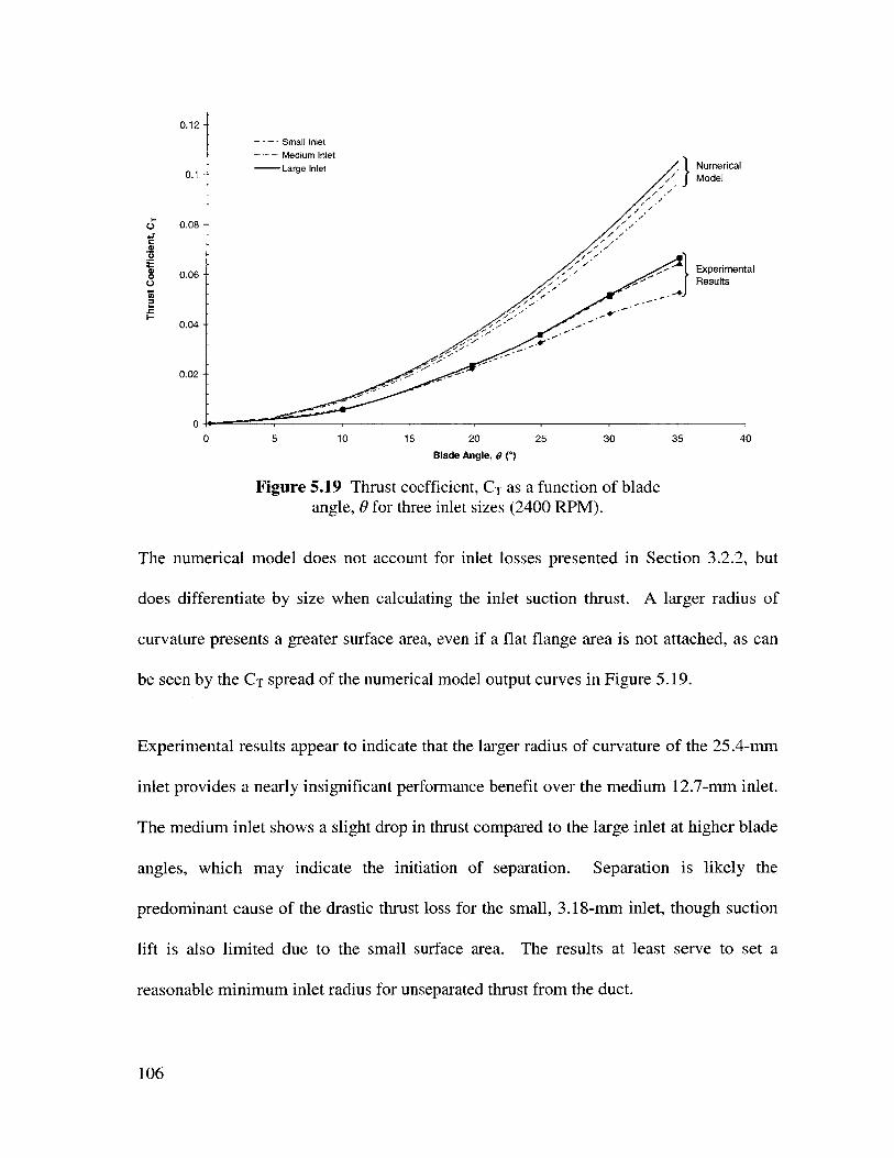
Figure 5.19 Thrust coefficient, CT as a function of blade angle, 0 for three inlet sizes (2400R P M ). ................................................................................................................................... 106
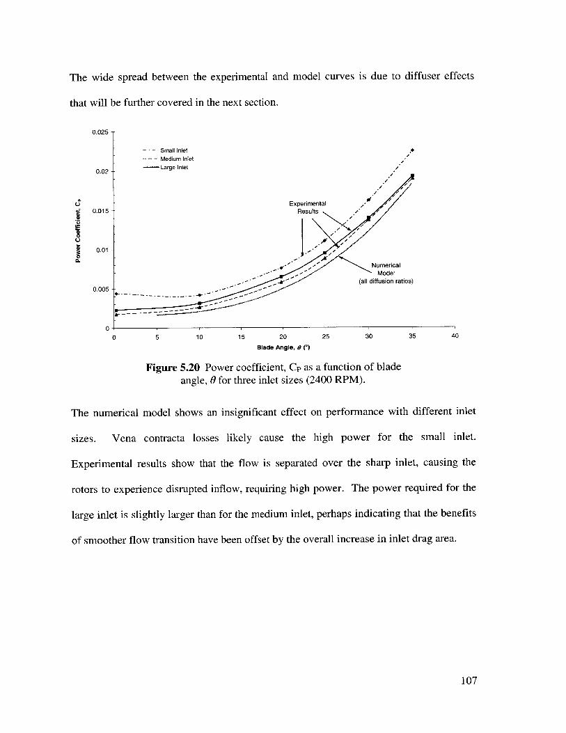
Figure 5.20 Power coefficient, Cr as a function of blade angle, 0 for three inlet sizes (2400R P M ). ................................................................................................................................... 10 7
Figure 5.21 Thrus coefficient, CT as a function of inlet size, r, (2400 RPM). ............................ 108
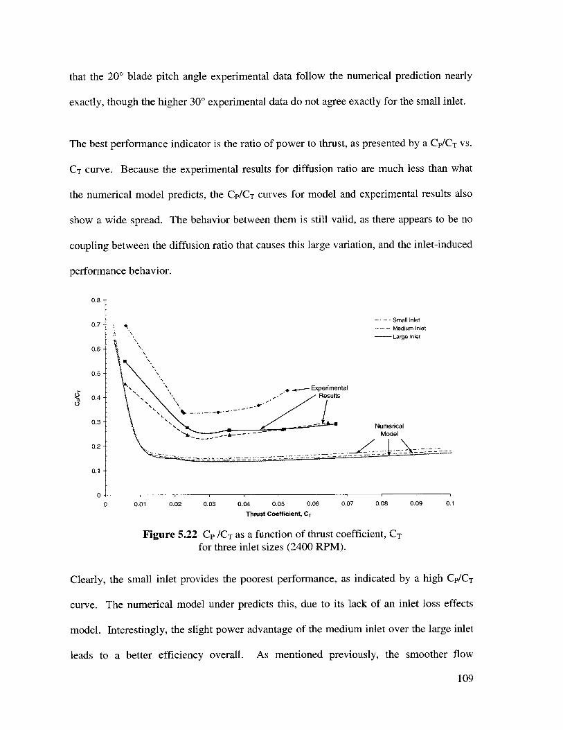
Figure 5.22 CP /CT as a function of thrust coefficient, CT for three inlet sizes (2400 RPM)...... 109
Figure 5.23 Thrust coefficient, CT as a function of blade angle, 0 for flanged and unflangedmedium inlets (25 mm flange, 1800 RPM). ......................................................................... 110
Figure 5.24 Thrust coefficient, CT as a function of blade angle, 0 for three diffuser ratios (2400R P M ).................................................................................................................................... 111
Figure 5.25 Thrust coefficient, CT as a function of diffusion ratio (2400 RPM)....................... 112
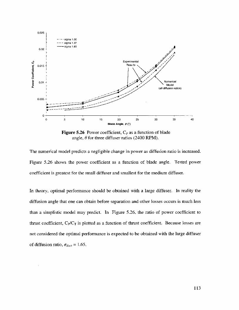
Figure 5.26 Power coefficient, Cr as a function of blade angle, 0 for three diffuser ratios (2400R P M ). ................................................................................................................................... 113
Figure 5.27 Cp/CT as a function of thrust coefficient, CT for three diffuser ratios (2400 RPM)............................................................................................................................................... 1 14
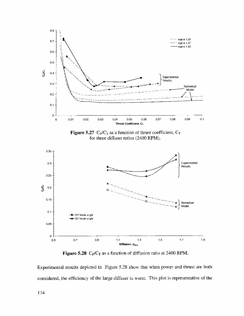
Figure 5.28 CP/CT as a function of diffusion ratio at 2400 RPM............................................... 114
List of TablesTable 2.1 UAV aircraft type comparison................................................................................. 20
Table 4.1 Diffuser dimensions (see Figure 4.8)........................................................................ 74
T able 5.1 T est m atrix.................................................................................................................... 82
Table 5.2 Motor and driveline data.......................................................................................... 86
Table 5.3 Differential collective calibration test...................................................................... 88
Table A-1: Inertial Motors Specifications. .................................................................................. 121
8
Page 9
Chapter 1: Introduction
Many civil and military uses exist for a man-portable aerial reconnaissance vehicle
capable of vertical takeoff, high-speed horizontal flight, hover and vertical landing. The
Perching Unmanned Aerial Vehicle (PUAV), developed at the Charles Stark Draper
Laboratory was designed to meet these requirements while remaining small and light
enough to be carried in a backpack for close tactical surveillance support.
A ducted propeller design was chosen to allow a very small footprint while minimizing
the danger to users of the aircraft. It was believed that traditional ducted aircraft designs
are lacking in their ability to transition to high-speed forward flight. This is usually
accomplished by the aircraft slowly pitching forward such that the initially vertical axis
approaches horizontal in the forward direction of flight. Aircraft stall and loss of control
authority has been a historical problem with this type of transition. A unique double
flight mode was conceived for the PUAV in which the vehicle would climb vertically to
altitude, and then pull out of a dive in the opposite flow direction (see Figure 1.2 (a)).
Landing would be accomplished by reversing the direction of thrust and rotating the
vehicle toward the ground (see Figure 1.2 (b)). In this manner, both take-off and landing
would use gravity to control vehicle speed, while minimizing the angle of attack of the
vehicle and reducing the opportunity for stalled flight. The bi-directional flow required
9
Page 10
for such flight necessitated careful aerodynamic design of the duct, in addition to the
need for the rotor system to reverse the direction of thrust on command.
Figure 1.1 The PUAV Alpha II prototype.
(a)
I(b)
Figure 1.2 Takeoff (a) and landing (b) of the PUAV.
10
r-Tr 0 r-lEr 0Liff. Lif
Page 11
The PUAV was designed in a short time span with minimal expense. The brief
timeframe limited the depth of aerodynamic design possible. Following construction of a
prototype, initial tests showed that performance was worse than expected, believed due in
part to disturbed airflow over the duct. In the hover mode, air entered the duct past a
small radius inlet lip, which acted as the annular airfoil trailing edge in forward flight.
The leading edge of the annular airfoil then acted as the hover duct exit. Powered tests
while observing wool tufts disturbed by the turbulent airflow were inconclusive in
determination of separation, but it was believed that thrust was being lost to stall at the
inlet, disturbed flow entering the rotor disk, and further separation at the radiused exit. A
review of the design was proposed, which would create a numerical aerodynamic model
of the duct and rotors to be used in a redesigned vehicle. Aerodynamic testing would
then be performed to verify the model before implementation.
The primary focus of the work presented herein is to model the airflow of a small ducted
aircraft and substantiate the numerical model with experimental results. Chapter 2
highlights the history and current stable of vertical takeoff UAVs, and then describes the
background of the PUAV project. The third chapter covers the theory behind helicopter
and ducted vehicle flight, with specific coverage of diffused and contrarotating coaxial
ducted aerodynamics. The test vehicle constructed for these tests, described in Chapter 4,
allows the introduction of several inlet mouths and exit diffusers and can be run for
indefinite lengths of time using a tethered electric motor. The test article is not limited to
the bi-directional architecture of the PUAV, but is based on a similar sized vehicle.
11
Page 12
The PUAV project has been successful in producing useful design lessons, as well as
yielding hover test results that can be used in the redesign of the PUAV airframe. The
results and test methods may be extended to other ducted thrust and lift producing
applications at the Draper Laboratory as well, including forward velocity wind tunnel
tests.
The significant results of this program are listed below:
" Ducted propeller test vehicle
o Engine driven drive train for 1 or 2 rotors
o Electric motor driven drive train for 1 or 2 rotors
o Servo driven variable pitch mechanism for ] or 2 rotors
o Reconfigurable duct inlets
o Reconfigurable diffuser section
" Data collection apparatus
o LabView based data acquisition
o Integration of load cell, RPM, current and voltage sensors, and servoposition
o Development of pitot-tube based wake surveys
" Ducted rotor hover test data
o Range of tested variables (duct geometry, collective, RPM, # of rotors)
e Numerical ducted rotor model
o Matlab based simulation tool
o Validation tests performed on test data
12
Page 13
Chapter 2: Background and History
2.1 Design Requirements
The evolution of battle has brought about a widespread use of strategic and medium to
large scale tactical surveillance platforms, ranging from space-born satellite assets and
large, high-altitude reconnaissance airplanes like the RQ-4A Global Hawk, to smaller
fixed wing tactical vehicles such as the RQ-1A Predator. At the beginning of the twenty-
first century the utilization of Vertical Takeoff and Landing (VTOL) Unmanned Aerial
Vehicles (UAVs) and Micro Aerial Vehicles (MAVs) is still quite immature.
Although there exist many manned and unmanned theatre-wide surveillance platforms
and medium range tactical support aircraft, there is a need to provide real-time close
support surveillance capability to the foot soldier, who must fight in an increasingly
complex battlefield. Such a vehicle could peer through windows, around corners, and
over hills to provide the soldier with an enhanced level of situational awareness, with
much reduced risk of injury or death. Visual sensors could provide information on
terrain outlay, hostile troop and civilian movements, as well as hidden weapons that may
not be detectable from longer range or directly above, and therefore beyond the capability
of most long-range surveillance platforms.
13
Page 14
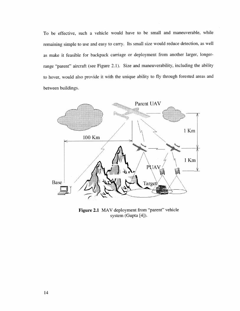
To be effective, such a vehicle would have to be small and maneuverable, while
remaining simple to use and easy to carry. Its small size would reduce detection, as well
as make it feasible for backpack carriage or deployment from another larger, longer-
range "parent" aircraft (see Figure 2.1). Size and maneuverability, including the ability
to hover, would also provide it with the unique ability to fly through forested areas and
between buildings.
Parent UAV
1Km
100 Km
Figue 21 MAepomntfom"aen"veil
'7
//1' ~ 'I4/ PVA~ ~ I Km
Base liz " ~Target
Figure 2.1 MAV deployment from "parent" vehiclesystem (Gupta [4]).
14
Page 15
Based on perceived interest of the US Defense Department, the Charles Stark Draper
Laboratory set the following requirements at the onset of this program:
e No larger than 10 inches (maximum linear dimension)
e Video downlink capable
e VTOL flight capable
e Capable of 20-minute flight duration
e Capable of hovering in winds of at least 5 mph
e Capable of transitioning to high speed (40+ mph)forward flight
The Perching UAV (PUAV) was designed to fulfill most of these requirements. Its
dimensional constraints were partially waived for a first iteration, with the intention that
future designs evolve into a smaller aircraft. The diameter fell within the constraints but
the height exceeded the limits by several inches.
2.2 Survey of Similar Aircraft
2.2.1 History of Vertical Takeoff Aircraft
As with helicopters, the melding of vertical takeoff and high speed forward flight
capabilities in unmanned vehicles has been the bain of UAV designers. The history of
small vertical takeoff aerial vehicles is broad and varied, and filled with many failed
attempts at an economical, high performance vehicle.
The origins of unmanned aerial vehicles harken back to the late nineteenth century, when
Douglas Archibald used a kite to carry aloft a camera with which to take reconnaissance
photographs. During the Great War, Charles Kettering developed a biplane aerial
torpedo that contained a rudimentary control system, making it the first guided cruise
15
Page 16
missile. Many other designs have followed, mostly driven by the need for military
reconnaissance, munitions delivery and targeting.
On the fourteenth of September 1939, Igor Sikorsky brought the helicopter into being
with the first flight of his VS-300. Powered by a Franklin 75hp engine driving a three-
bladed rotor, this open-frame, single seat helicopter was soon developed into the VS-
316A. The VS-316A, with military designation XR-4 and YR-4A, had an enclosed two-
place cabin, a slightly larger rotor, and was powered by a more powerful 175hp engine.
Four years after the flight of his first helicopter, Sikorsky's VS-316A went into
production. Today helicopters are used in myriad manned and unmanned operations that
would otherwise be difficult or impossible.
The first vertical takeoff and landing (VTOL) UAV to become operational was the
Gyrodyne QH-50 DASH (Drone Anti-Submarine Helicopter), introduced by the Navy in
1963. These UAVs provided standoff capabilities to ships by delivering torpedoes to
targets far from the fleet. Since that time many VTOL UAVs, mostly helicopters, have
been put to use around the world in civilian and military operations.
2.2.2 Current Vertical Takeoff UAVs
The military use of vertical takeoff UAVs has been most noticeable in the maritime
arena, where small ship decks preclude the normal operation of airplanes. While the US
Navy operates fixed-wing aircraft like the RQ-2A Pioneer from the decks of ships, the
rocket assisted launch and net-capture recovery of such vehicles is difficult and
dangerous.
16
Page 17
After disappointment in the results of the Tactical UAV (TUAV) competition, a fixed-
wing UAV program that sought to focus Army, Navy and Marine UAV needs, the Navy
and Marine Corps decided to develop their own VTOL UAV program. The early 1990s
saw several programs, including the joint US-Canada Maritime VTOL UAV System
(MAVUS), the domestic Tilt-Rotor UAV System (TRUS), and the Vertical Launch And
Recovery (VLAR) program. In 1997 the VTOL Demonstrator program was initiated to
determine the state of maritime VTOL UAV capability. The Bell Eagle Eye tilt rotor,
SAIC Vigilante helicopter, and Bombardier (formerly Canadair) CL-327 Guardian
contrarotating coaxial rotor helicopter competed while several other platforms including
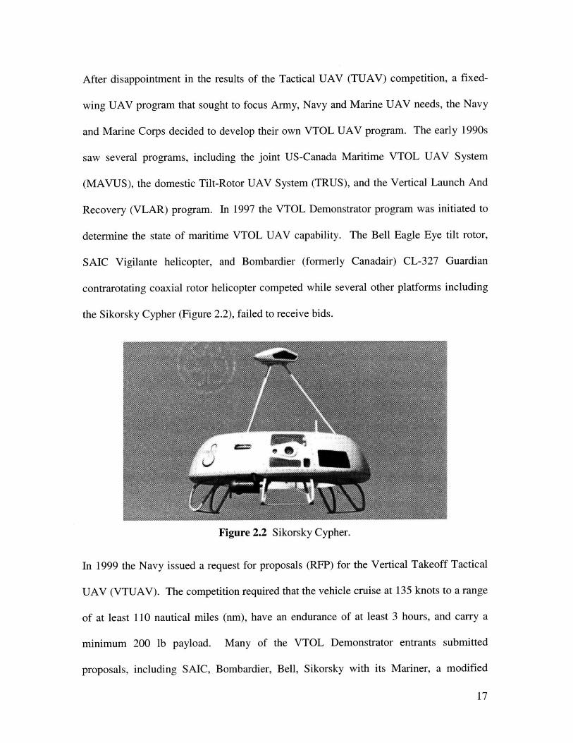
the Sikorsky Cypher (Figure 2.2), failed to receive bids.
Figure 2.2 Sikorsky Cypher.
In 1999 the Navy issued a request for proposals (RFP) for the Vertical Takeoff Tactical
UAV (VTUAV). The competition required that the vehicle cruise at 135 knots to a range
of at least 110 nautical miles (nm), have an endurance of at least 3 hours, and carry a
minimum 200 lb payload. Many of the VTOL Demonstrator entrants submitted
proposals, including SAIC, Bombardier, Bell, Sikorsky with its Mariner, a modified
17
Page 18
version of Cypher with wings, and Northrop Grumman with the Model 379 Fire Scout.
The Fire Scout, a modified version of the Schweizer 333 four-place manned turbine
helicopter, won the competition. It has since received go-ahead for Low-Rate Initial
Production (LRIP).
The Defense Advanced Research Projects Agency (DARPA) currently has two
development and flight demonstration contracts under the Advanced Air Vehicle (AAV)
program. One, the Frontier Systems A160 Hummingbird seeks to achieve high (48 hour)
endurance and long (2000 nm) range through the use of a variable speed rotor system,
allowing optimal cruise efficiency. The Boeing Dragonfly Canard Rotor/Wing (CRW)
stop rotor aircraft also hopes to achieve airplane-like range and vertical takeoff
capability. The design is based on a stoppable warm-cycle reaction-driven rotor system
that can act as a wing when stopped for high-speed (350-400 kt) cruise flight.
While the above programs seek to raise the bar in terms of aircraft performance, they are
far too large and expensive to be used for over-the-hill personal tactical reconnaissance.
Although the Sikorsky Cypher may fulfill some requirements, it is still incompatible with
most packable combat missions. Several small helicopter-based UAV systems have been
developed around the world including the Austrian Schiebel Camcopter, the French
Survey-Copter and Techno Sud Vigilant, and the US Aerocam. Many of these designs
are used for filming and other civilian tasks, and have not been designed for the rigors of
field combat use.
Ducted VTOL platforms have also made some headway. The standing piloted
Hummingbird VTOL observation platform has been converted to the unmanned Hornet
18
Page 19
by the Israeli company AD&D. Powered by four 22 horsepower engines turning two
contrarotating 3-bladed rotors within a 2.2 m duct, it can carry a payload of 115 kg.
Smaller vehicles include the aforementioned Cypher, which has a thick donut-shaped
duct with external dimensions similar to the Hornet. Its payload and gross weight are
approximately half as great as the Hornet, however.
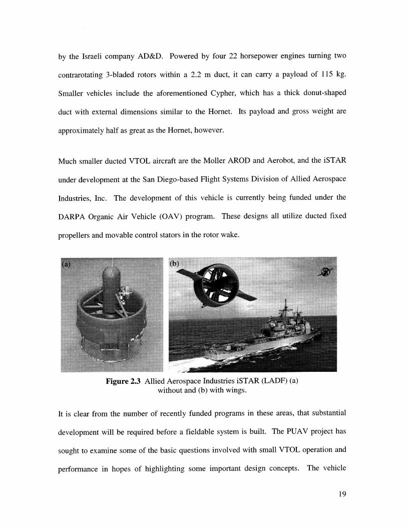
Much smaller ducted VTOL aircraft are the Moller AROD and Aerobot, and the iSTAR
under development at the San Diego-based Flight Systems Division of Allied Aerospace
Industries, Inc. The development of this vehicle is currently being funded under the
DARPA Organic Air Vehicle (OAV) program. These designs all utilize ducted fixed
propellers and movable control stators in the rotor wake.
. .. . ..... A E
Figure 2.3 Allied Aerospace Industries iSTAR (LADF) (a)without and (b) with wings.
It is clear from the number of recently funded programs in these areas, that substantial
development will be required before a fieldable system is built. The PUAV project has
sought to examine some of the basic questions involved with small VTOL operation and
performance in hopes of highlighting some important design concepts. The vehicle
19
Page 20
design differs from other concepts in its use of variable pitch contrarotating rotors. This
project was focused on examining the performance benefits of this type of system over
simpler and lighter, yet less efficient fixed pitch single rotor systems.
2.3 PUAV Development Evolution
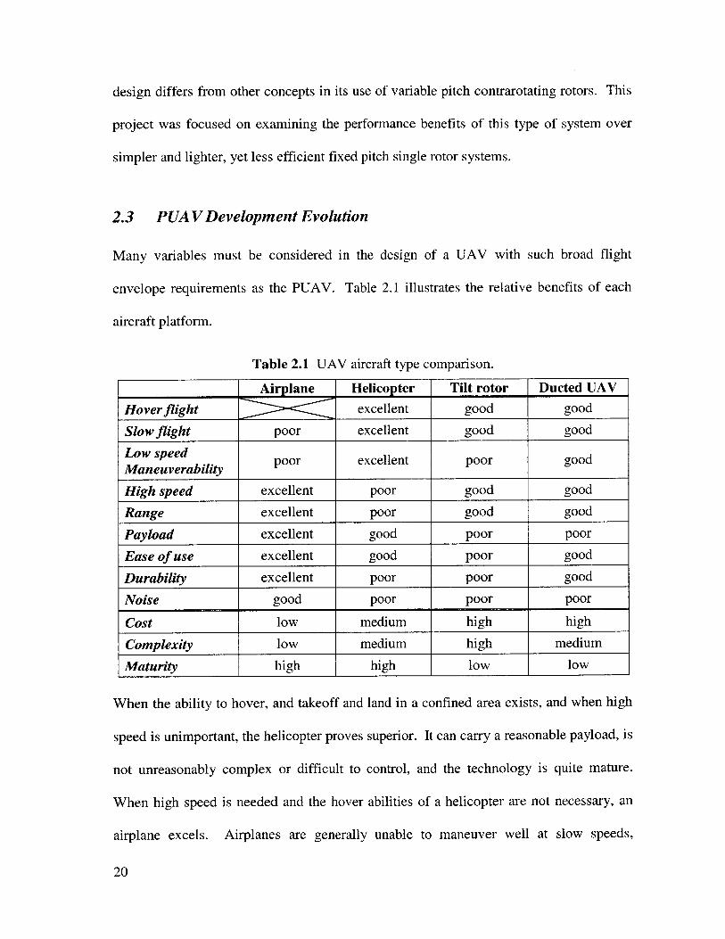
Many variables must be considered in the design of a UAV with such broad flight
envelope requirements as the PUAV. Table 2.1 illustrates the relative benefits of each
aircraft platform.
Table 2.1 UAV aircraft type comparison.
Airplane Helicopter Tilt rotor Ducted UAV
Hoverflight excellent good good
Slow flight poor excellent good good
Low speed poor excellent poor goodManeuverability
High speed excellent poor good good
Range excellent poor good good
Payload excellent good poor poor
Ease of use excellent good poor good
Durability excellent poor poor good
Noise good poor poor poor
Cost low medium high high
Complexity low medium high medium
Maturity high high low low
When the ability to hover, and takeoff and land in a confined area exists, and when high
speed is unimportant, the helicopter proves superior. It can carry a reasonable payload, is
not unreasonably complex or difficult to control, and the technology is quite mature.
When high speed is needed and the hover abilities of a helicopter are not necessary, an
airplane excels. Airplanes are generally unable to maneuver well at slow speeds,
20
Page 21
however. This is especially true with small airplanes such as Micro Aerial Vehicles
(MAVs) with wingspans of less than 15 cm, as their wing loading is often high, requiring
higher velocities and therefore large turning radii. For most requirements however,
either an airplane or a helicopter can provide the necessary flight profile.
If the need for hover and high-speed flight are combined, a hybrid design must be used.
The tilt rotor combines the rotors of a helicopter and the wings of an airplane to provide
both airplane speed and helicopter hover capability. Due to complexity and the small
size of the wings and rotors, neither mode performs as well as a comparable airplane or
helicopter, respectively, though. Ducted vehicles like the iSTAR and PUAV also use a
combination of a rotor and wing, though in this case the wing is shaped as a ring
surrounding the rotors, enhancing thrust and providing lift during cruise flight. Some
ducted vehicles do not rotate to transition to forward flight, .simply flying edgewise like a
helicopter. The Sikorsky Cypher flies in this manner, with its winged sister aircraft, the
Cypher II and Mariner designed to yield enhanced cruise performance.
Although other designs, including stoppable rotor helicopters, like the Boeing Dragonfly
that transition to airplane flight when airborne, are under development, the four aircraft
types listed in Table 2.1 cover the gamut of aircraft types currently available for
reconnaissance missions. Due to the requirement for small size, hover flight, fast forward
cruise, and good maneuverability, a ducted VTOL UAV design was chosen for the
PUAV.
21
Page 22
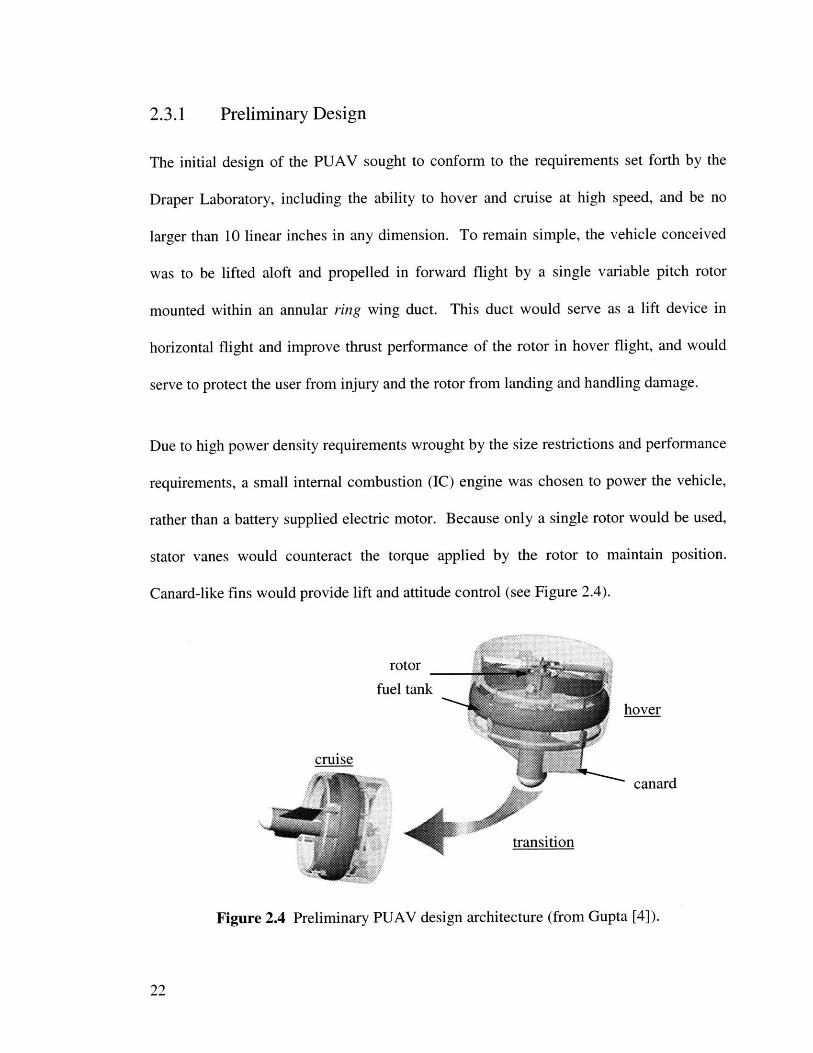
2.3.1 Preliminary Design
The initial design of the PUAV sought to conform to the requirements set forth by the
Draper Laboratory, including the ability to hover and cruise at high speed, and be no
larger than 10 linear inches in any dimension. To remain simple, the vehicle conceived
was to be lifted aloft and propelled in forward flight by a single variable pitch rotor
mounted within an annular ring wing duct. This duct would serve as a lift device in
horizontal flight and improve thrust performance of the rotor in hover flight, and would
serve to protect the user from injury and the rotor from landing and handling damage.
Due to high power density requirements wrought by the size restrictions and performance
requirements, a small internal combustion (IC) engine was chosen to power the vehicle,
rather than a battery supplied electric motor. Because only a single rotor would be used,
stator vanes would counteract the torque applied by the rotor to maintain position.
Canard-like fins would provide lift and attitude control (see Figure 2.4).
rotor
fuel tank
hover
cruise
canard
transition
Figure 2.4 Preliminary PUAV design architecture (from Gupta [4]).
22
Page 23
Analysis of the control authority
provide insufficient pitch control.
further forward, where they could
Alpha prototype.
supplied by the canards indicated that they would
A redesign was thus begun that brought the canards
act about a greater moment arm. This became the
2.3.2 Alpha Prototype Design
Due to shortcomings in the initial design, a revised architecture was developed. Because
too much stability reliance was being put on the anti-torque stator vanes, a coaxial design
was conceived. This would allow the two rotors to turn in opposite directions, canceling
the torques produced by each. By varying the collective blade pitch angles differentially
between the rotors, a yaw torque in hover or roll torque in forward flight could be
accomplished, reducing the load on control vanes and fins.
The need for high control authority brought the canard fins further away from the duct.
For cruise flight this created the adverse affect of putting the aerodynamic center forward
of the center of mass, creating instability in pitch. To alleviate pitch instability, the mass
was moved further forward by extending the center fore body and installing four
cylindrical pods that could act as mount points for the canards, accommodate the canard
control mechanisms, and house the batteries required for the radio control receiver and
servos. The stilt-like pods could also serve as landing gear for a hover landing.
Research references
the rotor diameter.
difficult. To fit the
indicated an optimal rotor spacing of approximately 10 percent of
Packaging constraints made placement of the engine critical and
rotors and engine in the duct section left almost no room for the
23
Page 24
gearbox that would have to reverse the direction of one of the rotors. With sufficient
volume within the duct annulus to do so, a gearbox was placed in the duct. One drive
shaft ran outward from the center-mounted engine to the gearbox, and another shaft ran
between the rotors to a bifurcating gearbox that fed the rotors in opposite directions from
one another. The external gearbox location also made engine starting easier.
engine
gearbox rotorsrotors
canards. . .. . .canard
controlpayload servos
batteries
SLA pods
Figure 2.5 Alpha I prototype.
Due to testing difficulties of the IC engine, a tethered electric motor was substituted for
initial tests. The vehicle was hung in its hover orientation from an overhead pulley
arrangement as depicted in Figure 2.6. A line ran through a pair of pulleys where it was
attached to a large weight, with a mass greater than the vehicle mass. This mass was
placed on a tared scale, so that when the vehicle was not producing thrust the scale
displayed a weight of zero. As thrust increased, the apparent weight increased, indicating
the thrust of the vehicle. This test was only valid for thrust less than the vehicle weight.
24
Page 25
Figure 2.6 Alpha I prototype thrust test apparatus (from Gupta [4]).
The tests proved that the electric motor provided insufficient torque to drive the rotors at
a high blade angle and at high speed. It was also clear that the weight of the vehicle was
too great. Because the fore body components, including the main body and four pods,
were made using the stereo lithographic apparatus (SLA) process, which creates a part
out of heavy and brittle epoxy resin, they were chosen as the best components from
which to pare weight.
25
Page 26
enginestarting cone
gearbox rotors
caard
canardscotlservos
batteries
carbon fiber pods
Figure 2.7 Alpha II prototype, with redesigned forebody.
The redesign, illustrated in Figure 2.7, incorporated the same general dimensions, though
the shape of the pods and the construction of all the components were changed. The
canard control servos were placed within the streamlined carbon fiber epoxy composite
pods, reducing air drag and the chance of damage. The main body and canards were also
made of carbon fiber composite. The weight of the entire structure was reduced from
approximately 500 grams, about 40 percent of the overall vehicle weight, to less than 350
grams.
Once the fore body redesign was complete and the engine was reinstalled, tests were run.
The thrust test apparatus comprised of a cantilevered beam mounted to a bearing,
allowing free motion about the vertical axis. The vehicle was mounted to the end of the
beam and a line and pulley system arranged to a tared weight atop a precision scale
26
Page 27
provided a measurement of thrust (see Figure 2.8). Testing proved difficult, though
largely to the recalcitrant engine.
pivot ple
starting cone
Figure 2.8 Alpha II thrust test apparatus.
2.3.3 Beta Prototype Design
Alpha II prototype thrust testing with the IC engine resulted in many failed components,
as the torque produced by the engine overstressed the gear train components. The single
cylinder 0.25 and 0.32 cubic inch displacement engines used for testing create very high
periodic torques that vary in magnitude and direction through rotation. As the crankshaft
turns, the drive train and flywheel must provide the torque to pull the piston through top
dead center. Shortly thereafter the engine fires and drives the flywheel drive train with
tremendous torque, reversing the drive train load. Brass gears were deformed and steel
keyways were sheared due to these periodic loads. This effect was most predominant
during starting and shutdown, when the relative speeds of the gear train and engine were
disparate.
27
Page 28
To alleviate some of the stresses incurred during shutdown, a one-way clutch was
installed on the outer gearbox. This allowed the rotors to freewheel when the engine
came to a brisk halt, eliminating stress that had previously sheared gear teeth and
keyways. The small IC engines used for testing ran equally well in either direction
however, and would often start backwards because no load was applied in the reverse
direction of rotation.
engineflywheel
engine cradle c fiber
carbon fiber
gearbox tray .. supportstruts
reduction gear
rotors
Alpha IIfore body
Figure 2.9 Beta prototype.
The redesigned gear train of the Beta prototype sought to address the starting and strength
concerns. The parts count for the new design (Figure 2.9) was drastically reduced, and
steel gears were substituted for brass gears. It became evident in testing that the engine
was torque limited, and because sufficient thrust was believed possible at speeds of 6000-
8000 RPM, half that of the engine's maximum power speed, a gear reduction was
28
Page 29
deemed necessary. A gear reduction was designed into the outer gearbox tray, allowing
engine to rotor gear ratios of 1:1 or 2:1.
The Beta prototype retained all other structural components of the Alpha II prototype.
Unlike the previous designs, the Beta drive train did not include an extension of the
engine shaft protruding from the duct. Starting was to be accomplished through the use
of a rubber puck-like disk pushed against the small flywheel of the drive train. This
method proved unfeasible. The standard OS .32 SX-H engine was replaced with a .32
SX-HX, identical to the .32 SX-H except in its pull-start mechanism attached to the rear
of the crankcase. Although it added weight, the pull-start mechanism would be beneficial
for field operations, negating the need for an external electric power source to supply an
electric starter.
Engine starting, even with the revised pull start, still proved nearly impossible due to the
drive train drag and low inertia. A decision was made to abandon the use of small IC
engines in place of a much more robust motor. While the motor size and weight was
incapable of flight, testing could easily be accomplished for all relevant geometries and
conditions.
The evolution of the decision has resulted in a robust test vehicle, suitable for effectively
characterizing the thrust performance and power load of the ducted rotor system. The use
of a large electric motor provides a power source sufficient for testing the performance
envelope of the design. Engine selection for the final flight vehicle can be completed
after requirements have been set, based on knowledge gained from tests with the electric
motor.
29
Page 30
[ THIS PAGE INTENTIONALLY LEFT BLANK ]
30
Page 31
Chapter 3: Theoretical Performance
3.1 Rotorcraft Aerodynamics
The performance of a rotor or propeller can be calculated using several methods, each
with differing accuracy. Momentum theory treats the rotor as an actuator disk, which can
maintain a pressure differential between the top and bottom surfaces. More accurate
models treat the disk as multiple concentric rings, but the fundamental theory remains
unchanged. Blade element theory treats the rotor blades as wing sections and computes
the local lift and drag produced by a section of each blade as a function of the local
induced velocity and blade orientation.
Although the momentum and blade element theories presented herein have been
developed from Johnson [6] and Leishman [10], they are both commonly used and
accepted. Both models are complicated by the convoluted flow around two
contrarotating coaxial rotors surrounded by a duct, as is the case with the PUAV.
3.1.1 Momentum Theory
A propeller or rotor produces thrust by accelerating a mass of fluid. The rotors of a
helicopter in hover draw still air from above and propel it downward, yielding a vertical
upward thrust. An airplane propeller draws in air traveling at a relative velocity equal to
31
Page 32
the airplane speed through the air, and accelerates it rearward to produce thrust. The
PUAV shall perform both tasks, although only the hover regime will be discussed in this
report.
Momentum theory allows the calculation of thrust and power by way of three
conservation equations. Mass must be conserved within the system, usually defined by a
control volume enveloping the rotor and upstream and downstream wake.
Station [0] PO = Patn, VO =0
Station [1] '\ \ \ R dRotoi disk/Station [2] \ ' P2, V2 = Vi
P3 =Pann, V3 = OStation [3]
Figure 3.1 Helicopter rotor control volume.
Variable subscripts denote the station, or location across the control volume, of interest.
Conservation of mass states that the mass flux through the system, with surface S, air
density p and velocity vector V , must be zero
<fgpV -d95= 0. (3-1)S
32
Page 33
Conservation of momentum allows the calculation of thrust from the summation of
momentum flux through the same control volume
T = pd5+ TpV -dV, (3-2)S S
where p is pressure.
Based on the conservation of energy for the system, the work needed to produce thrust is
found to be
W =4f p1dI. (3-3)S
Note that this work manifests itself as the change in kinetic energy that accompanies the
production of thrust. Power, P, is work per unit of time, or the time rate of change of
Equation (3-3).
Equation (3-1) means that the mass of air flowing into the control volume of Figure 3.1 at
Station 0 is equal to the mass flowing out at Station 3 and also the same as the mass flow
through the rotor at Stations 1 and 2,
th = ffpV -d5 = pV -d = fJpV -d (3-4) (a)
th = pAIv, = pA3 o (3-4) (b)
where vi is the inflow velocity, or induced velocity at the rotor and CO is the downstream
velocity (see Figure 3.1).
Recalling that thrust is the rate of momentum flux through the system, Equation (3-2)
becomes
F =T = p(V -d5V - ffp(V -d5V. (3-5)
33
Page 34
The pressure term is not included because both the inlet and exit ends of the control
volume are at an equal atmospheric pressure.
Because the velocity far upstream is zero, Equation (3-5) becomes simply
T = fp(Y -dS )Y = rhw .
The power required to produce this thrust is defined by using Equation (3-3) as
P = J{ p(Y. dSY -2 _p(Y -)Y I.
The power required in hover, or work done by the rotor per unit of time, is
P =Tvi.
(3-6)
(3-7)
(3-8)
The velocity upstream is zero; therefore the second term of Equation (3-7) is dropped.
This leads to the equality
Tv, =Irhco =(pAvi )W2,
which, when combined with Equation (3-6) yields
v, =4(0.
(3-9)
(3-10)
From Equation (3-4) (b) we see that the wake area A3 is half the rotor disk area A.
Combining this result with Equation (3-8) leads to
T = rhmw= 2pA vf.
Rearranging,
T
We can now solve for the induced power Pi, as a function of thrust T.
P = Tvi = T T TX2pA Jp
(3-11)
(3-12)
(3-13)
34
Page 35
Note that the power is a function of 1/V2A . Neglecting friction losses as well as weight
and structural problems, an infinitely large rotor would yield the minimum induced
power. The viscous drag of such a large rotor actually reduces the optimal size, and
operational, weight and cost constraints further reduce the 'best' rotor size for a
helicopter.
The disk loading, DL of a helicopter is the ratio of the total thrust to rotor disk area
DL = A = 2pv2, (3-14)
while the power loading, PL defines the amount of thrust for a given power
PL= = =pA - - =- 1 . (3-15)P T DL
Its reciprocal 1/PL is equal to the induced velocity, and is often referred to as the rotor
efficiency parameter. Note that Equation (3-15) accounts only for induced power P,.
Blade friction and other losses increase the power consumption.
Profile drag, D, multiplied by the local blade velocity and radius can be integrated along
the blade for all Nb blades to yield profile power.
Po =Nbf(Dy)dy (3-16)0
The radial position along the blade is denoted by y, while the tip radius is R.
The drag is defined by
D(y)=PVI cal CCd 142 Cs (3-17)2 2
35
Page 36
For the simplified case of constant Cd independent of Reynold's number Re and Mach
number M, the profile power becomes
1 =P, = -NbQ 3 C R.
8 (3-18)
While Equations (3-14) and (3-15) provide a way of comparing general vehicle
parameters, non-dimensionalization allows direct comparison of many more specific
parameters.
The thrust and power coefficients are defined in terms of thrust and power, disk area A,
and rotor tip speed
CTT T
pAV,7, pA( QR) (3-19)
(3-20)and Ci = ', P ' ,pAVti pA(i R)3
where the rotor tip speed is calculated by multiplying the rotor frequency Q, by the rotor
radius R.
Using the profile power from Equation (3-18) and using the non-dimensionalization
shown above, we find the profile power coefficient to be
C 1 p RCPO 8 pAC 3 R 3
NbcR)CA C, (3-21) (a)
(3-21) (b)Crotor Cd
8
where the rotor solidity
- Ablades NcR NbcR Nb cirotor A ,R
2 - R
is the ratio of total blade area to disk area.
(3-22)
36
Page 37
The induced velocity can be non-dimensionalized in terms of Q and R as well.
vi =AQR (3-23)
Rearranging yields
_i 1 T (3-24)R1 R 2pA 2pA(QR)2 2
where A, is the induced inflow ratio.
Using a modified version of Equation (3-15) and Equation (3-24) leads to the power
coefficient as a function of thrust coefficient
C YC, =C Ai =--- (3-25)
In reality, the induced power is slightly higher than theory predicts due to non-ideal
effects. In the above equations we have assumed that the inflow is uniform, tip losses
and wake swirl do not exist, and there are an infinite number of blades. Experimental
results for helicopters show that a linear induced power correction factor, K, reasonably
accounts for these losses. A typical value of K for a helicopter is 1.15.
C Y2C = CT (3-26)
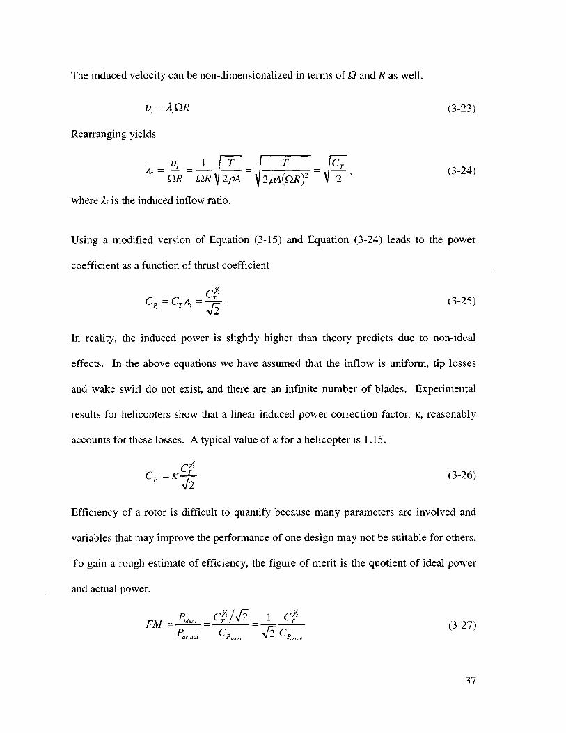
Efficiency of a rotor is difficult to quantify because many parameters are involved and
variables that may improve the performance of one design may not be suitable for others.
To gain a rough estimate of efficiency, the figure of merit is the quotient of ideal power
and actual power.
P C /-,2 I CYFM= =deal = -f T (3-27)
Pactual C Cual acual
37
Page 38
If one substitutes the induced plus the profile power for Pactual, the following theoretical
result is found
FM = 5 2
C 0t,, Cd(3-28)
The numerator denotes the ideal power while the denominator contains induced power
and profile power terms from Equations (3-26) and (3-21) (b) respectively. Note that as
the thrust coefficient increases FM tends towards 1/K. For this reason, the figure of merit
is only applicable for direct comparison between two rotors of equal CT.
U.
1.8-
1.6-
1.4 -
1.2-
1 -
0.8 -
0.6 -
0.4 -
0.2 -
0*-
- sigma 1.00- - - sigma 1.37- - sigma 1.65
/ -..
~. ,
/
/7
0.02 0.04 0.06 0.08 0.1 0.12Thrust Coefficient, CT
Figure 3.2 Theoretical PUAV figure of merit for differentdiffusion ratios.
Typically, a
performance.
figure of merit in the range 0.7 to 0.8 represents good helicopter
38
0 0.14
Page 39
3.1.2 Blade Element Theory
The blade element theory (BET) considers a rotor as the finite sum of two-dimensional
airfoils. The rotor aerodynamic forces may be calculated radially along the blade and the
lift and drag integrated to yield vertical thrust and shaft torque required to turn the rotor.
A single blade is considered to represent the behavior of all blades and performance
calculations may be accomplished through a simple multiplication by the number of
blades. Closed-form solutions can be calculated for certain conditions such as uniform
inflow with a simply twisted blade, while iterative solutions are needed for more complex
configurations.
Blade element theory allows the calculation of forces, moments and fluid velocities on
the blade and in the wake, which cannot be done with momentum theory. This
distinctive capability is important as a base from which most other rotorcraft analysis is
performed. Specific blade profiles can be analyzed using BET, as well as the influence
of the wake on thrust performance. Noise and vibration prediction is also possible with
the information that comes from such a model.
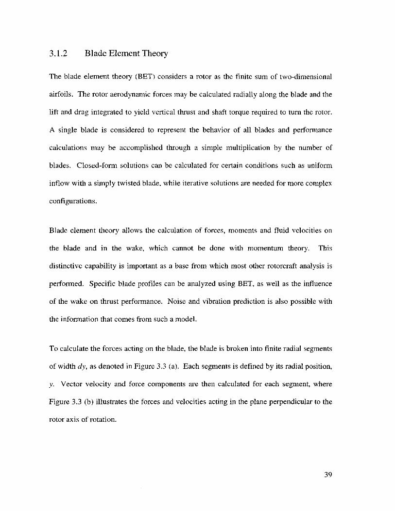
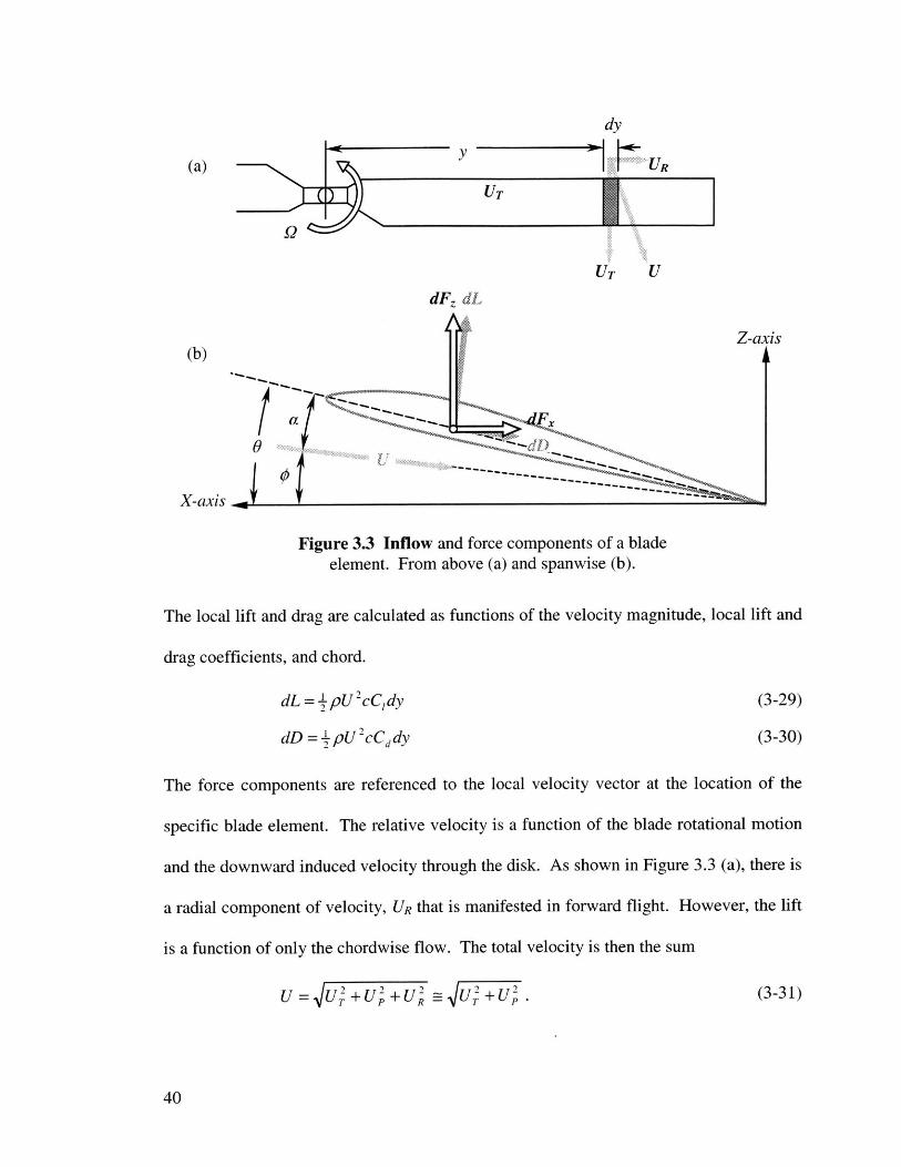
To calculate the forces acting on the blade, the blade is broken into finite radial segments
of width dy, as denoted in Figure 3.3 (a). Each segments is defined by its radial position,
y. Vector velocity and force components are then calculated for each segment, where
Figure 3.3 (b) illustrates the forces and velocities acting in the plane perpendicular to the
rotor axis of rotation.
39
Page 40
dyya
(a) R
Ur
UT U
dFz dL
Z-axis(b)
Xaxis
Figure 3.3 Inflow and force components of a bladeelement. From above (a) and spanwise (b).
The local lift and drag are calculated as functions of the velocity magnitude, local lift and
drag coefficients, and chord.
dL = _ pU 2 cCidy (3-29)
dD=_+pU 2cCdy (3-30)
The force components are referenced to the local velocity vector at the location of the
specific blade element. The relative velocity is a function of the blade rotational motion
and the downward induced velocity through the disk. As shown in Figure 3.3 (a), there is
a radial component of velocity, UR that is manifested in forward flight. However, the lift
is a function of only the chordwise flow. The total velocity is then the sum
U = U2 +U2 +U ~ U1 +U. (3-31)
40
Page 41
We consider only airflow perpendicular to the blade axis, represented by the rightmost
part of (3-31) for simple blade element theory analysis. The general inflow angle from
the induced flow is then
# = tan _- U1 . (3-32)
For a helicopter rotor the induced angle is generally small, so a small angle assumption is
valid.
S~ U P/Ur (3-33)
The angle of attack, as illustrated in Figure 3.3 is then the difference between the blade
angle 0 and inflow angle #.
a=6-# (3-34)
C=OL for q<<1 (3-.35)UT
The lift and drag coefficients of the blade element are functions of angle of attack, a, and
are also dependent upon Reynolds number, Re, and Mach number, M, although the latter
two effects are sometimes neglected. The lift coefficient is typically modeled as a linear
function of a, with a slope C, of 2;r. Drag coefficient is modeled as a quadratic function
of a. According to Johnson [6], a typical drag coefficient for helicopter blades is
Cd = 0.0087 -0.0216a+0.400a2. (3-36)
Although local blade forces in the blade axis or inflow axis are occasionally useful, one
generally cares more about the total forces on the rotor hub and helicopter. First, we will
calculate the forces in the rotor hub axis. This yields the vertical thrust force F-, acting
41
Page 42
on the blade and hub parallel to the rotor shaft axis, and the radial drag force Fx, acting
normal to the blade axis and rotor shaft axis.
dF =dLcos # -dDsin # (3-37)
dF, = dL sin #+ dD cos # (3-38)
The vertical thrust increment is then the sum of the local vertical force dF for all Nb
blades. The incremental torque is found similarly, except the x-axis is of concern and the
force is multiplied by the moment arm y of the location. Power is torque multiplied by
radial velocity, D.
dT = N dF = N dL= N PU 2 cCdy
dQ = NbdF y = Nb (ML+dD)y
dP = dQ -Q = NbdFvyQ = Nb(ML+dD)yQ
= NbpU cpC, + Cd )ydy
(3-39)
(3-40)
(3-41)
The last term in each of the above equations is valid for small angles where sin # ~ # and
cos ~ 1. The thrust, torque and power are the integral sums of the above equations over
the radius, R of the blades.
R R Ru2ccdT = fdT = fPNbdL = pNb U 2cdy
0 y=O y=0
P = IPNb U c(#C, +Cd )"ydyy=0
(3-42)
(3-43)
The incremental thrust, torque and power can also be used to find their equivalent
coefficients.
N dL N (UcCidy) 1!C )c2dCr = R) , = 2 =-CI( L d ---pA p ()rR2 (R)2 2 /rR R R
Nb (vL + dD)y
pA(QR)2 R
(3-44)
(3-45)
42
Page 43
dC - Nb (/dL + dD)yt2 (3-46)pA(QR )
In the non-dimensional form, the rotor radius becomes r = y/R and UIQR=QyIQR=y/R=r.
Recalling that the rotor solidity ,row, = (Nbc)/(,rR), we can simplify Equation (3-44) to
dCT = arotor C1r 2 dr (3-47)2
The torque and power coefficients follow similarly and are equal.
dC = dC =Nb ( (C + Cd )IY2R3 (3-48)
__1
Srotor(#CI + Cd )r 3dr2
The induced inflow ratio, 2, = I/R , comes from Equation (3-24).
1= -- -- = - - (3-49)' OR fy ( YR UrP R-)=O
Because # = 1,/r, the power coefficients becomes
dCp = I ,rtr (A Cr 2 +C dr' P. (3-50)2
Also, for the linear lift curve case where C, = a -C1, and recalling that
a = 9 = 9 - , /r , the thrust coefficient follows as
dCT rotor i (or 2 -A.rkdr. (3-51)2
Integrating Equations (3-47) and (3-50) yields the thrust and power coefficient.
CT = 2 rotor Cirdr (3-52)0
C=y2c07otor J(Ac r 2 + Cdr')dr (3-53)0
43
Page 44
Blade element theory and momentum theory can be combined to provide the inflow
profile A, (r). The thrust can be found based on momentum theory, where the
incremental area dA = 2zydy is an annulus of width dy at a discretized radius y.
dT = 2pv,2dA = 4frpvydy (3-54)
In coefficient form this becomes
dC = 4A2 rdr,
while the induced power coefficient is
dC, = 4A'rdr.
Equating results from the BET (Equations (3-50) and (3-56)) gives
(3-55)
(3-56)
(3-57)dCr =44rdr = '""" C" (or -- id.2
Solving Equation (3-57) results in the quadratic equation for the inflow profile as a
function of r
a C 32(r '" '"I 1+ 9r -1 ,
16 L ,ror,.C(3-58)
where Uroor, 0, and C, can all be functions of r. This combined theory is called blade
element momentum theory (BEMT). The induced velocity and thrust can also be
computed iteratively, which is often the only option when complex blade geometries and
lift and drag coefficients are considered.
3.1.3 Coaxial Momentum Theory
As a first approximation to the case of two coaxial rotors within a duct, we will consider
the case of unducted contrarotating coaxial rotors as they are used on many Russian
44
Page 45
Kamov Design Bureau helicopters. The two rotors are considered to be closely spaced,
so that the wake of the upper rotor has not contracted when it passes through the second
rotor. This means that the area of each rotor is equal (Arotor = Arotr = A). Based on
continuity (Equation (3-4) (b)) the induced velocity through each rotor must be equal. If
the area and induced velocity are equal we can reasonably assume that the thrust is
equally distributed between the two rotors. The total thrust is then 2T, where T is the
individual thrust from each rotor.
2T(V, )Co=ial -- - = (3-59)
2pA pA
Substituting into Equation (3-13) we find that the total induced power between the two
rotors is
(P, )cx = 2T(vi )coaial = 2T T -2T (2T) (3-60)ideal FpA 4pA .vjr2 '
K ,t i(2T )Yand (PI )coaxial = KKWt (P )coaxial = , (3-61)
where Equation (3-61) includes correction factors to account for non-ideal losses.
Due to the halved effective disk area of a coaxial rotor compared to two non-overlapping
rotors of the same size, the interference induced losses amount to an increase in induced
power of rAi = -Th = 1.41. Tests of actual aircraft show that interference actually yields
values of Kint that are closer to 1.16 for coaxial helicopters. The difference is due in part
to vertical rotor separation. Helicopters with coaxial rotors tend to have large rotor
separation, causing the second rotor to be only partially in the nearly fully developed
wake of the first. In theory, if the second rotor is within the fully developed wake of the
45
Page 46
first, such as far downstream, the theoretical interference factor is 1.28. In this case only
half the rotor is in the wake of the first rotor, while the outer half of the rotor area is in
free air. For the ducted rotor case, one may assume that there is negligible contraction,
causing the rotors to behave as though they were closely spaced.
Another effect of contrarotation is reduction of swirl in the wake. The regular induced
power correction coefficient K generally accounts for the energy lost in the rotor wake
and will be reduced if swirl is diminished. It is possible that the seemingly small
experimentally determined interference coefficient Ki,,t, of 1.16 mentioned above, was
calculated with the assumption of a regular induced power correction factor K, of 1.15,
rather than a smaller K that accounts for swirl. The total correction KKi,, may have
therefore been incorrectly distributed between K and Ki,,.
The profile power is theoretically unchanged from the single rotor case, but the total rotor
solidity for a pair of equal rotors is twice that of the single rotor. This has the effect of
doubling the profile power losses,
( )coaia = pA(QR)32 rotor Cdj (3-62)8,
where -roor is the solidity of a single rotor.
3.1.4 Ducted Rotor Performance
This section has thus far covered the momentum theory model of two closely separated
rotors of equal dimension and shared thrust. While the duct provides the benefit of
46
Page 47
reduced or eliminated tip vortices, thus reducing K, its primary purpose is the boost in
efficiency that comes with diffusion, or spreading of the induced flow from the rotor disk.
Upstream rotorArotor
Downstream rotor
Awake
Figure 3.4 Ducted rotor with diffuser exit.
Incorporating a diffuser at the exit of a ducted rotor allows the effective wake area to be
changed while maintaining a fixed rotor disk area. From Equations (3-8) and (3-11), we
know that the power is dependent upon the induced velocity passing through the rotor
disk, vi, while the thrust is a function of the total change in momentum, and thus
dependent upon the far wake velocity o and area Awake. The diffuser allows these
parameters to be altered to better suit performance and efficiency objectives.
A rotor = A (3-63)
Awake = Od uctA (3-64)
where aduct, is the duct diffusion ratio.
Therefore, we can rewrite Equation (3-4) (b) as
th = pA vi = PAwakeW = Ucr pA o. (3-65)
47
Page 48
This means that
V.C= ' . (3-66)Oduct
Note that uduct is not based on the ratio of rotor disk area to duct exit area, but rather to the
area of the far wake. For an unducted rotor, Uduct = 0.5.
Considering again that thrust is the time rate of momentum flux through the system, the
total thrust is
Titl = T,,,t, + Tu,t = rh0). (3-67)
Using the constitutive equation, this becomes
A ,Total = p V. (3-68)
aduct
The induced velocity is then
_ ~duet"ota (3-69)pA
Applying the Bernoulli equation at the inlet
PO = P1 +{ pv2 = Pain, (3-70)
and the exit
P 2 + 7 pvi = p3 +3 pa = Parm + j02 (3-71)
allows the computation of the rotor thrust, Trtor.
Trotor = A(Ap) = A(P2 - P1 ) (3-72)
Solving for p, and P2 and substituting the results into Equation (3-72) yields
To,, = IpAaf. (3-73)
48
Page 49
The contribution to thrust can best be seen by its ratio to total thrust
Trotor 2 (3-74)
Total pA vi> 2v 2oduct
Although thrust is produced by both the duct and the rotors, induced and blade profile
power are absorbed only from the rotors. Thus
( )r Ttotal d ttotalrotor rotor diuct/ pA
TY2 2auct A(3-75)total
Dividing Equation (3-75) by the induced power for an unducted rotor becomes
total
(i )ducted 4
)TdutP _ 1- 3 (3-76)
(i )untjucteci Total (3-76)
Equation (3-76) illustrates the effect of duct diffusion on efficiency. The above
theoretical equations do not account for blade profile drag losses or skin friction drag on
the duct. It should also be noted that obtaining large duct diffusion is difficult, as the
adverse pressure gradient of a diffuser yields significant losses and the final wake area is
often less than expected. This will be covered in Section 3.2.3.
3.2 Other Inlet and Diffuser Effects
The inlet, duct, and diffuser constrain the inlet and exit airflow. The pressure and shear
stresses imparted on the vehicle surfaces by the air cause drag and can also provide
thrust. Skin friction drag is generally less important for higher Reynolds numbers than
pressure drag at the diffuser and inside the inlet lip, caused by flow separation and an
49
Page 50
adverse pressure gradient. If a sharp inlet is installed, the air has difficulty maneuvering
around a sharp corner and can separate, thus causing losses. A conical diffuser creates an
inherent adverse pressure gradient, which leads to losses as well.
3.2.1 Inlet Thrust Augmentation
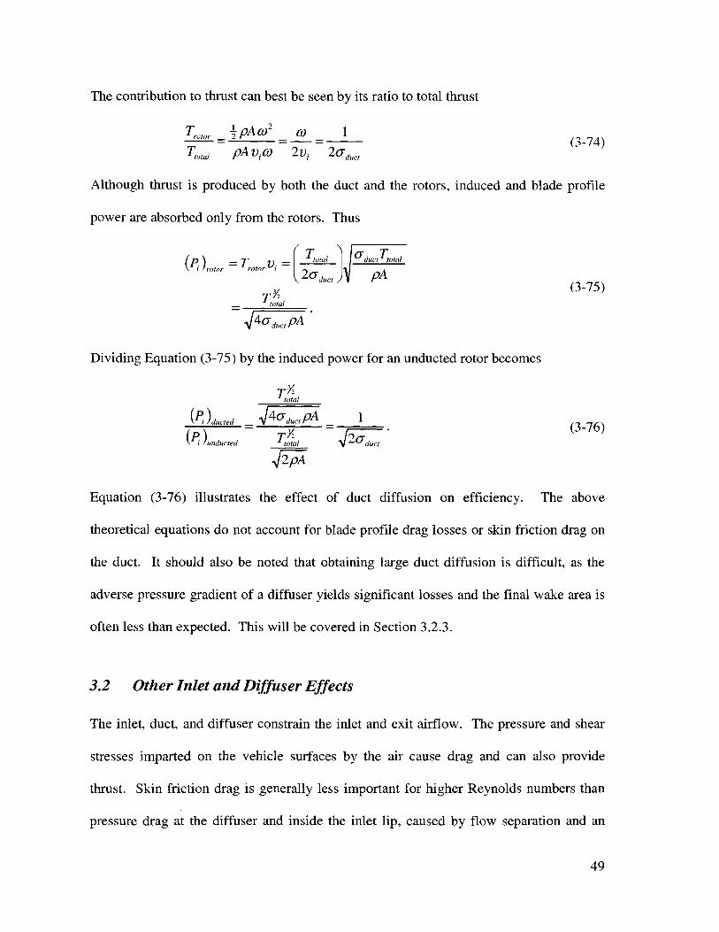
Like a wing, airflow over the inlet surface causes the inlet to experience lift. Through the
Bernoulli equation, one can follow a streamline entering the rotors to calculate the
pressure along the profile as a function of the velocity. A simplistic model is based on
semi-concentric sphere caps that are normal to the inlet and flange surfaces where they
meet (Figure 3.5). The surface area, S, of each sphere cap defines the velocity ratio
between the surface area S, and the duct or rotor area, A, for each streamline. The
velocity on a given sphere cap is thus the induced velocity at that streamline where it
inters the rotor multiplied by the ratio of rotor disk area to sphere cap surface area.
(a) (b)
Figure 3.5 Streamlines (a), and pressure distribution(b) over the inlet.
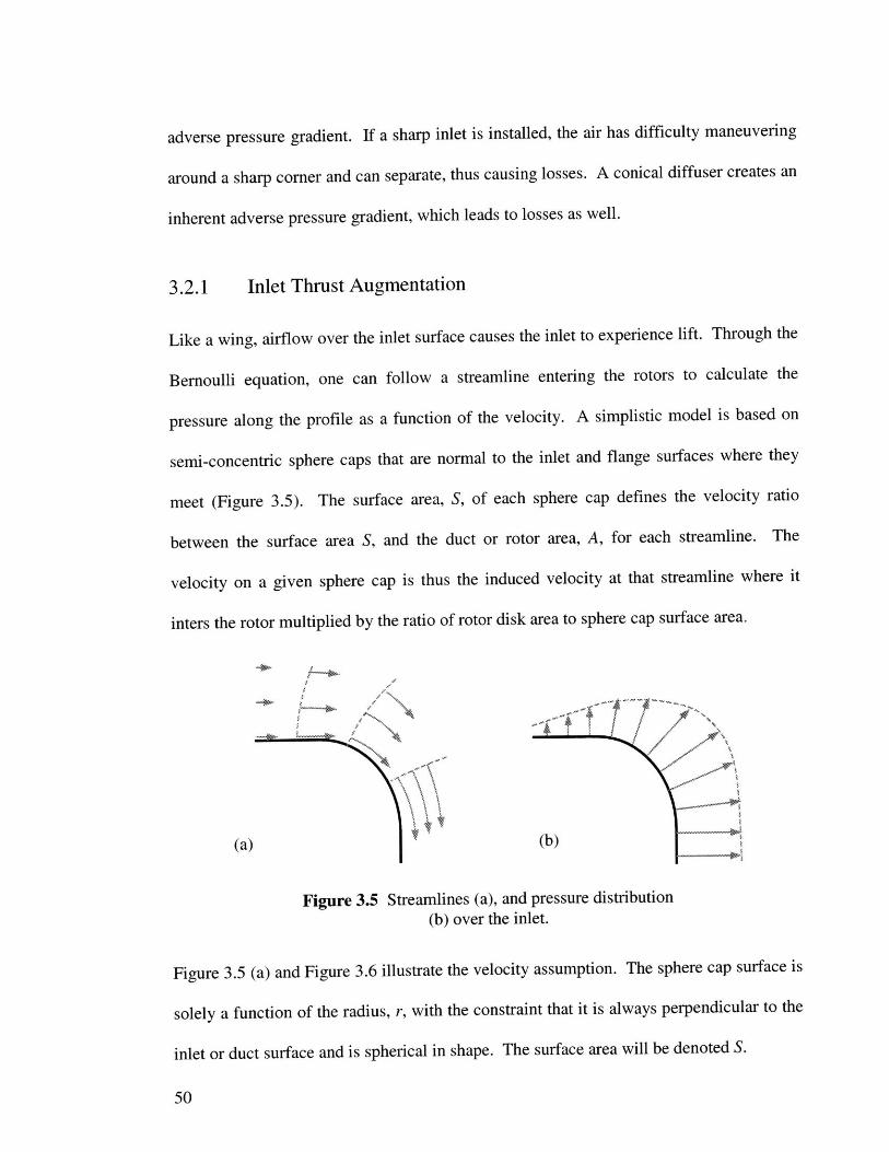
Figure 3.5 (a) and Figure 3.6 illustrate the velocity assumption. The sphere cap surface is
solely a function of the radius, r, with the constraint that it is always perpendicular to the
inlet or duct surface and is spherical in shape. The surface area will be denoted S.
50
Page 51
The axial thrust produced by this lift is simply the product integral of pressure and area in
the axial direction. Note that all forces acting radially cancel through symmetry.
(2;r) (r 1+r+f)
Tnit = f f(Ap)(I -n4rd9 (3-77)0 (r=rd)
The dot product of the duct axis vector i and the local surface normal n translates the
pressure and area into of the duct axis.
From Bernoulli,
Parn +0 = Pinet + j pVj, (3-7 8)
AP = Parm - Piniet = ± PiP, et (3-79)
Assuming that the velocity profile through the surface S is everywhere proportional to the
velocity at the duct of surface area A, continuity can be used to yield the velocity at the
surface as a function of r and v 2 .
rh = pA Vi = PSVnlet
A = r (3-80)S S
For the limit where r = rd, the duct radius, the surface area S becomes the duct area A and
Vinet = v,. When r > (rd + ri), where r; is the inlet lip radius, the surface area S becomes
that of a hemisphere, with surface area S = 21r2
A sphere cap is the surface obtained when the portion of a sphere above a certain plane is
considered. The surface area of a sphere cap is S = 2rrh, where r is the radius of the
circle created by the intersection of the sphere and the plane, and h is the distance
between the center of the circle and the top of the sphere. In this case, r is the same radial
dimension used in the integral of Equation (3-77).
51
Page 52
Surface, S
h
rr 1z
Figure 3.6 Inlet surface area geometry.
Using the geometry of Figure 3.6, the surface area S can be solved as a function of radial
position r, duct radius rd, and inlet lip radius of curvature ri. The radius of the sphere
defining S is re which can be found from
r2 +h2
r = 2h .(3-81)C 2h
One can solve for the sphere radius (or in the two-dimensional case displayed, the circle
radius), from the duct geometry as
r rr- rr,r r 2 - + rd - r (r - rd)(2r, + r - r) (3-82)
Similarly, a scalar pressure magnitude correction based on the forward component of the
surface normal vector
m r (r - r)(2r, + rd -r)m = n -1 (3-83)
is equivalent to the dot product of the surface normal vector and the duct axis vector.
52
Page 53
Using Equations (3-86) and (3-82), the surface area S for the condition rd < r < rd + r, is
=27r(r-rr r 2 22sli, = ,)~ d)- 2 = )r ' . (3-84)r~ -_(r + rd - r 2 (2r, + rd -)
If a flange is attached to the periphery of the inlet, a greater surface area can be used to
augment thrust through lift. The flange will be considered to have a radial dimension
from the inlet radius of length f. For the flanged case, recall that the surface S, which
defines the velocity profile, is that of a hemisphere.
Sflage =2xr 2 (3-85)
The total inlet thrust is then the sum of two integrals of thrust in the axial direction. From
Equations (3-80), (3-84) and (3-85), the total thrust can be calculated.
(2)r) (rd+r+f)
Tinet = f,,mlet )drdo = Th,+ Tflange (3-86)0 (r=rd)
First, based on the surface S perpendicular to the lip surface, the thrust for rd <r d +
T ,rd+ r' +(2r rd - d)2 (r - rdX2 . +rdr(
rrd
The flange thrust based on the hemisphere of radius r for r> rd +
Tflage 2=2nx r-drY PV 2 2 dr
(3-88)
Tflange =ipzV f -d drr=rd +r
Combining Equations (3-87) and (3-88) results in a total thrust of
r=rdr+r r
53
Page 54
The above equations are based on several broad assumptions that have been defined
before their formulation. However, the choice of v, is not predefined and has a strong
impact on the thrust result. A conservative method would have the inlet surface velocity
distribution defined as a function of the average disk induced velocity, while a less
conservative approach would define the surface velocity in terms of the high rotor tip
induced velocity nearest the duct wall. The choice of v, is especially significant for an
untwisted ducted rotor in which the induced velocity is high at the blade tips.
Experimental surface pressure distribution plots for a ducted fan, presented by Black,
Wainauski, and Rohrbach [3], appear to validate the general theory of inlet suction lift,
and indicate that the above model is overly conservative, even in the case where tip
induced velocity is used.
3.2.2 Inlet Losses
The previous section examined the benefits of a large inlet mouth. In considering the
design of an inlet duct, it should be noted that size and weight constraints often prohibit a
large inlet lip radius of curvature, however. The effect of inlet thrust augmentation
decays with radius as the velocity reduces, while the skin friction drag increases. Thus,
there is a point at which the thrust lost to drag equals the thrust gained by augmentation.
Operational and external dimension constraints will usually limit the size more than drag
considerations.
54
Page 55
Figure 3.7 Vena contracta.
When the flow separates from the inlet surface, the effective area is decreased, causing
the velocity at the throat of the duct to increase. Although not much energy is dissipated
in the acceleration of a fluid, the deceleration that must occur as the flow once again
conforms to the duct saps energy in the form of a head loss. The head loss can be solved
as a pressure loss
Ap = KL (p (3-90)
where KL is the loss coefficient. Vena contracta losses are difficult to model. Thus, loss
coefficients are found experimentally as a function of rijet/Dduce. In the case of a tube
inlet, the loss coefficient (KL) ranges from near zero for a large radius, to 0.5 in the case
of a sharp inlet lip.
Substituting the induced velocity from Equation (3-12) and solving for the lost thrust TL,
it is possible to obtain the thrust lost as a function of total thrust.
TL =ApA = K jL Z" )A (3-91)S2
TL K L (3-92)T 4
55
Page 56
For a sharp-lipped inlet the thrust lost due to separation and the vena contracta will be
approximately 12.5 percent of the total thrust.
Several studies have investigated the effects of inlet lip radius on performance of a ducted
propulsor such as the PUAV. Taylor [17], found that the thrust efficiency is not greatly
affected for inlets with a lip radius to duct diameter ratio great than 0.6. His results and
those based on the theory developed from Munson et al [13] are both presented in Figure
3.8 below. Taylor's results indicate a much more drastic drop in performance as the lip
radius is brought near zero. This increase in losses due to inlet geometry is probably due
to severe lip separation, and the turbulent airflow that is created by the sharp inlet as the
flow enters the rotor disk.
0.9 - .- KL 4 )
1/2 inch 1 inch
0.8- 1/8th inch inlet radius inlet radius
inlet radius
0.7 } experimental resultsfrom Taylor
0.6-- - - 16* blade angle
- 24* blade angle
U 0.4
0.3-
0.2-
0.1 -
00 0.02 0.04 0.06 0.08 0.1 0.12 0.14 0.16 0.18
r/D
Figure 3.8 Thrust losses due to sharp inlet curvature.
56
Page 57
3.2.3 Duct and Diffuser Losses
The duct and diffuser are segments of a tube with internal flow and its attendant losses.
Because of its short length, the straight duct portion of the PUAV only exhibits small skin
friction losses. However, the adverse pressure gradient of the diffuser causes more
substantial performance losses.
Like the inlet losses, diffuser losses can be accounted for by using Equations (3-90) and
(3-91). However, the area and velocity are not simply the induced velocity and duct area,
respectively. In the case of a diffuser, the pressure drop occurs over the entire length
where the velocity decreases and area increases. Integration must be used to yield the
total drop. The result is similar.
TL (3-93)
T 4U(9
Though a longer, more gradual diffuser will reduce separation, the skin friction will
reduce the efficiency. An optimal diffusion angle for a given ratio will thus exist. As in
the case of the inlet, experimental results must be used due to the complex nature of
decelerating fluids.
3.3 PUA V Numerical Model
Because we are considering the ducted contrarotating coaxial rotor, three effects must be
considered that aren't significant to helicopters. First, the duct diffuser changes the wake
flow, increasing the induced flow at the rotor but adding to the overall thrust of the
vehicle. Second, the tip vortices that dilute the performance of a helicopter are
constrained by the duct, diminishing the need to account for tip effects. Finally, the swirl
57
Page 58
of the first rotor is not fully wasted in the wake. Instead, it increases the angle of attack
and velocity of the second rotor. Another point to consider is one of computational
simplification. Because of its large rotor diameter and low disk loading, the inflow angle
on a helicopter rotor is low and the trigonometric functions of the inflow angle can be
approximated by their small angle equivalents. The PUAV and other small, high-disk
loading aircraft maintain large blade angles and inflow ratios, which are usually beyond
the scope of small angle simplification.
The PUAV numerical model used to compare with experimental results is a dimensional
blade element momentum theory model graphically illustrated in Figure 3.9, which
includes duct diffusion. The lift coefficient used in the model is a linear function of a,
with slope 27c, while the drag coefficient is a quadratic function of a and Re in the form
Cd = (1.25+ 2.76a+ 44.8a 2 )Re-o346, which is based on the tested NHP tail rotor blade.
The blade grip will be considered as a cylinder with Cd =9 Re~0 5 due to the low
Reynolds number. Duct and inlet losses will not be calculated in the numerical model,
but should be considered qualitatively when comparing predicted results to experimental
results.
The induced and profile drag of the first rotor induces a swirl in the wake that the second
rotor encounters as a higher tangential velocity, Ur. This reduces the inflow angle
slightly, thus improving performance of the second rotor and recouping some of the
power that would be otherwise lost in a single rotor vehicle where the swirl would be
dissipated in the wake. The final swirl behind the second rotor is expected to be small,
and will therefore not be included in the numerical model.
58
Page 59
The flowchart illustrated below in Figure 3.9 outlines the process by which the Matlab-
based computational model calculates the performance of the PUAV. The model is first
initialized with a set of input conditions and an expected induced velocity. The latter can
be chosen randomly, and only serves to reduce the time to converge on a solution.
First, the total relative blade velocity, Reynolds number and angles are calculated based
on the rotational speed and induced velocity. The lift and drag coefficients can then be
found, which are used to find the local lift and drag component for each blade segment.
The local thrust values are then used to find the induced velocity for that segment. The
process iterates until the total thrust, the sum of all incremental thrust components,
converges to a steady value. The final induced velocity can then be used to find the inlet
thrust, which is added to the duct thrust to arrive at the total vehicle thrust.
Input: O(r), 6,C,,, c(r), RPM U(r) =f(or(r), RPM)Estimate: v;(r) #(r) =ft((;(r), RPM)
a(r) = 0(r) - #(r)Re(r) = f(U(r))
CL(r) =fta(r))Note: Each variable is a CD(r) =f(a(r), Re(r))
vector of size r x 1, dL(r) =f(c(r), U(r), CL(r)) vi(r) =f(dT(r),T(r),)where each cell defines dD(r) =f(c(r), U(r), CD(r))
the local conditions at dT(r) =f(#(r), CL(r), CD(r))
dP(r) =f(dD(r), y(r), RPM)that blade segment.
Trotor= YdT
Tduct f(Trotor, arotor)
Tiig =f3.i) Yes Converged? NoOutput:- P~r,. LdP
T,0,oi Tini,, + T,. ,
Figure 3.9 Computational Flowchart.
59
Page 60
[ THIS PAGE INTENTIONALLY LEFT BLANK ]
60
Page 61
Chapter 4: Experimental Test Apparatus
4.1 Drive Train
The drive train of the test article accomplishes the same tasks as that on the flight vehicle.
In both cases, the rotating drive train components provide the mechanical work to drive
the rotor blades, while the stationary components center the rotors within the duct. Due
to complications of a small internal combustion (IC) engine and the freedom of nearly
unlimited energy from an external power supply, an electric motor was substituted for
testing. The motor and power supply permit precise speed control while maintaining a
clean, low vibration environment unattainable with an IC engine.
4.1.1 Driveline
The driveline is the mechanical intermediary between the power source and the
aerodynamic blade components. It includes shafts, gears, bearings, guides and the
stationary components required to support all moving components. In the case of the
PUAV hover test article, the driveline acts to direct motor torque to the two rotor hubs
through six bearings and two gears as illustrated below.
61
Page 62
blade grips
Figure 4.1 Schematic diagram of PUAV hover test vehicledrive train.
The hover test article driveline was constructed out of machined aluminum and steel
components from the PUAV Beta Prototype. In an effort to reduce aerodynamic
blockage and drag, the lower profile lower spar of the Beta Prototype driveline was
substituted for the engine cradle, which normally contains the IC engine, flywheel and
one-way clutch. Although actual use in a flight vehicle will require that an engine be
mounted within the middle of the duct, aerodynamic testing would have been
complicated by such components. Future vehicles may entail fairings that would reduce
drag, but the design of such fairings would require further study and inclusion in these
tests would obscure the pure thrust results.
Low speed torque capabilities of the motor obviated the need for any reduction gearing
usually necessary for the high-revving IC engine. The large motor size also hindered any
internal mounting options that would have in any case added aerodynamic drag. The
motor was therefore mounted transverse to the duct in line with the secondary drive shaft.
Screwed to the end of the motor shaft is an aluminum machined coupling, with two lugs
comprised of small screw heads affixed to its peripheral face. The lugs match holes in
the large reduction spur gear mounted to the outer end of the secondary drive shaft. This
62
Page 63
attachment method allows for slight off-axis mounting and takes the form of a universal
joint, in additional to allowing some movement axial to the shafts.
--------.
- II
Figure 4.2 PUAV hover test vehicle drive train.
As in the case of the flight vehicle, the hover test article driveline center shaft is held by
two pairs of carbon fiber struts mounted axially from the spar end caps 120 degrees from
the secondary drive shaft and spars. The struts were screwed to the duct and stabilized by
epoxy. This axisymetric stiffening restricts bending strain of the spars and keeps the
center shaft exactly centered within the duct so that blade tip clearance remains constant
and blade-to-duct contact is curtailed.
Due to the ultimate need to reverse flow direction in the final flight vehicle, a symmetric,
zero-twist rotor blade profile was chosen for initial testing. Although blade twist and
camber would yield improved thrust and reduced power required in one direction,
performance would be unsuitable in the reverse direction. Negative twist, in which the
root is at a higher local blade angle than the tip, tends to equalize the angle of attack and
thus improve performance. Reversing the flow direction for the same blade yields an
63
Page 64
effective positive twist, in which the root has a lower blade angle than the tip. This could
cause the tip to stall while a small or negative root angle of attack would give reduced or
reversed thrust. An untwisted symmetric blade affords equal performance in either
direction, a compromise that must be made with the need to reverse the direction of flow
for the vehicle.
Carbon fiber foam core 29-mm chord NHP tail rotor blades were used for initial tests.
These symmetric blades have a thickness to chord ratio of 17%. Rotor solidity, otor, is
0.33.
7
+ Lift coefficient (XFOIL)-Linear lift curve slope (2pi)
* Cd at Re = 1e4o Cd at Re = 5e5 4,-
* *
4-----A- - --
03
0 --0
2 4
-~~'~3DD 0
6 8 10 12
Angle of attack, a (*)
NHP Tail rotor blade sectional lift and dragcoefficient.
0.U
C4)
.20)0
1.8-
1.6-
1.4-
1.2-
0.8-
0.6 -
0.4-
0.2 -
0-
0
Figure 4.3
14
64
Page 65
A linear lift curve with slope C = 2T was used to approximate the airfoil lift
coefficient. A higher fidelity model incorporating the airfoil stall characteristics could be
used in future versions if unreasonable angles of attack are seen.
The drag coefficient for an airfoil is often defined by a second degree Taylor series such
as Cd = 0.0087 - 0.021 6a + 0.400a 2 , with negligible compressibility or Reynolds number
effects for the case of a hovering helicopter rotor. Reynolds number affects the small
blades of the PUAV and like-sized vehicles, however. The Blasius flat plate skin friction
drag approximation considers the effects of Reynolds number on a flat surface. The skin
friction drag coefficient for a flat plate with laminar flow is
1.328C, = ,(4-1)
and for turbulent flow is
0.074C, = . (4-2)f ReY5
For Reynolds numbers in the range of 105 at which the PUAV rotor is running at the 75%
span, the skin friction drag coefficient is nearly the same for the laminar and turbulent
case. For the flat pitch case one could simply add the Reynolds number dependent skin
friction drag coefficient to the helicopter rotor Cd. However, this curve does not
reasonably fit the output data from XFOIL. A Reynolds number-dependent drag
coefficient was devised in the form
Cd = (a + ba+ ca2) (4-3)Re
65
Page 66
The best fit using the data from XFOIL was found with coefficients a = 1.25, b = 2.76,
c = 44.8 and d = 0.346. This equation fit is presented in Figure 4.3 by the dashed curves.
The blades are held by nylon tail rotor blade grips driven by Futaba S3102 high torque
micro servos. FMA S90 micro servos used in previous tests provided inadequate torque
capability. Centripetal loads on the blades were found to flatten them at high speed, and
swash plate and pushrod friction combined to require more torque than was available.
Without the need for small size, light weight, or high speed, the 51.4 oz-in S3102 servos
were mounted within an aluminum machined fixture fastened to the inlet end of the
center shaft for testing. One pushrod connects each servo to its respective swashplate and
rotor system. The swashplate transfers the actuation from the non-rotating frame of the
servos, to the rotating frame of the rotors and blades. The inlet rotor can be reached
directly, but the second rotor pushrod slides within the center shaft (see Figure 4.4).
downstream upstreamrotor rotor
servospushrods
downstream upstreamswashplate blade grips swashplate
Figure 4.4 Rotor collective control diagram.
66
Page 67
4.1.2 Test Motor
Previous vehicle tests were accomplished using the O.S. .32 SX-H helicopter engine and
.25 FX airplane engine. Controlled indoor tests required cumbersome exhaust handling,
and the noise, fuel spatter and vibration of the engine made testing difficult. Throttle
control was also problematic, and torque measurement during thrust production would
have required a complex strain gauge and commutator apparatus. Available engines were
also limited to a narrow speed and torque envelope. For these reasons, an electric motor
was chosen as superior for initial testing, with flight engine sizing to follow test data
analysis.
Vehicle tests of the preliminary prototype were accomplished using an Aveox 1409/4Y 4-
wind brushless electric motor. This rather small motor was capable of high speeds, but
was limited in its ability to output the power and low-end torque needed for a broad test
envelope. The motor was designed for use in model airplanes where cooling air would
provide heat dissipation. Early hover tests with the Aveox motor caused the motor
temperature to become alarmingly high. Continuous operation would therefore be
restricted to much lower loads than were required for a reasonable test matrix.
A custom Inertial Motors Corp. servomotor was obtained, with the capacity for high
torque output, yet limited to lower speeds than the Aveox motor (see Appendix A). The
heat dissipation capacity of the IMC motor without external cooling allows practically
indefinite use at moderate to high torque loads. Figure 4.5 graphically illustrates the
expected torque required and that available from the Aveox 1409/4Y and Inertial Motors
Corp. DC Motor. The Aveox 1409 motor data presented in the graph are based on a 50
67
Page 68
percent load limit. This was chosen as a practical maximum in consideration of the weak
heat dissipation capabilities of the motor and the poor airflow expected in the test vehicle.
+1 MC DC Motor (limit torque)
-0- Aveox 1409/4Y [2:1 gear ratio] (50% limit torque)--- Aveox 1409/4Y [3.7:1 gear ratio] (50% limit torque)
0 2000 4000 6000 8000 10000 12000
Output Speed (RPM)
Figure 4.5 RPM vs. torque available and required.
14000
According to analytic power estimates, the torque available from the IMC motor is
greater than that absorbed by the vehicle for all proposed tests (dotted curve of Figure
4.5). The IMC motor allows a wide testing envelope, the results of which will be used in
sizing a flight vehicle power source. A higher speed would have been desirable, but the
practical limit of 6000 RPM is satisfactory.
The IMC motor contains an optical position encoder that provides high fidelity motor
speed information. The 500-pulse/revolution square wave output signal can be viewed
on an oscilloscope, which in turn provides frequency in kilohertz.
68
1
0.9
0.8
0.7
EZ 0.6
0 0.5I-
0.40
0.3
0.2
0.1
00
Page 69
fkH(l000pulses)X( 1rev ->)(60sec (rev = RPM (4-4)sec 500pulses 1mn mn
The torque and power provided by the motor can be calculated using rotational speed,
input voltage, and current data. This negates any need for an external torque sensing
capability and also serves to crosscheck speed measurements provided by the optical
encoder.
The speed of the motor can be found in terms of the current I, voltage V, motor armature
resistance Ra, and speed constant Kv.
RPM = -IRJ (4-5)Ky
Note that the armature resistance causes a voltage drop when current is applied.
The output torque can be found with input voltage, current and motor RPM.
Tou = (I - iNL )K, - Kd RPM (4-6)
In this case, the no-load current, iNL, reduces the available current, the balance of which is
then multiplied by the torque constant KT. The second term refers to speed dependent
viscous damping of the motor, where Kd is the viscous damping torque constant. The
motor constants noted above can be obtained from the manufacturer. Calibration curves
were generated for the motor to validate these specifications, which are presented in
Section 5.2.1.
4.2 Duct Construction
The duct itself yields much of the performance gain of the expected ducted vehicle
layout. As covered in Section 3.1.2, air recirculation at the blade tips leads to loss of
69
Page 70
thrust and efficiency. This is especially important in a high disk loaded vehicle such as
the PUAV or any other small VTOL aerial vehicle with a high thrust coefficient. The
purpose of a duct is the reduction of tip vortices. To accomplish this, the tip gap must be
very small, on the order of 0.5% gap size to diameter. In the case of the PUAV, 0.5 mm
was a reasonable goal, a gap to diameter ratio of 0.22%. The inner surface of the duct
must also be smooth, as surface roughness leads to skin friction drag and waviness can
produce flow separation.
Beyond its aerodynamic function, the duct contains and retains most of the vehicle
components. Although the motor and driveline are mechanically fastened with screws,
bending strain of the secondary drive spars due to vibration of the rotors allow the rotors
to contact the duct. Axially placed carbon fiber struts impart stiffness in this dimension,
and provide a rigid link between the central driveline components and the duct. The
driveline was also stabilized by a 0.25-inch thick aluminum plate bonded within a cavity
extruded into the outer face of the duct. The plate was sandwiched between the duct and
the motor mount to act as a motor mount interface, with metal-to-metal contact on both
faces.
70
Page 71
Figure 4.6 Duct/drive train interface.
The duct is composed of three sections; the inner structural housing, the exit diffuser, and
the inlet. The inner section is made of ABS plastic using the Fusion Deposition
Modeling (FDM) prototyping method. The inner diameter is a constant 220 mm (8.7
inches) and the length is 102 mm (4 inches). Twenty-five millimeter (1-inch) wide
flanges adorn each end, with holes to allow mounting of various inlets and diffusers.
This flexible design also allows the straightforward incorporation of new inlets, diffusers
and constant diameter lengthening plugs for future investigations.
4.2.1 Inlets
Smooth rounded inlets allow air to enter a duct with minimal separation. At the extreme,
a sharp-lipped inlet causes the air to separate into a vena contracta, while an excessively
large radius inlet suffers from skin friction drag.
71
Page 72
Like the inner duct section, the test inlets are made of ABS using FDM. Their complex
curvatures are well suited to the method. Three sizes were chosen for testing, of which
one was further modified to examine the effects of inlet surface area on thrust
augmentation. This latter flanged inlet was constructed by attaching a thin ring-shaped
sheet of G-10 composite to the interface. It was bonded to the face of the ABS inlet with
minimal surface variation, which could have caused turbulence or separation losses.
The smallest inlet tested, theoretically expected to yield the poorest performance (see
Figure 3.8), has a lip radius of approximately 4 mm (0.125 in.). The ratio of lip radius to
inlet diameter is 0.014. This was the hover inlet radius on all previous flight vehicle
prototypes. The second inlet has a lip radius of curvature of 13 mm (0.5 in), yielding a
ratio of 0.057. A flanged test inlet has the same 13 mm lip radius, but has bonded to its
face a 25 mm (1 inch) wide flange (see Figure 4.7). Tests comparing operation with and
without the flange verified expectations that a small amount of thrust is produced by high
velocity inflow air passing over the flange, creating low pressure on its face.
The largest test inlet has a 25.4 mm (1 inch) radius of curvature, yielding a rather large
lip radius to inlet diameter ratio of 0.114. This was the baseline inlet with which the
various diffusers were tested. It is believed that this large radius is least affected by
separation, and will thus result in the most pure diffuser effects results.
72
Page 73
R
R25.74 mm
R12.70 mm
3.18 mm
110.51 mm
Figure 4.7 Section diagrams of four test inlets.
4.2.2 Exit Diffusers
The purpose of a diffuser is to reduce the exit velocity, which should yield improved
thrust efficiency at a slight cost to thrust for a given collective pitch setting. Section 3.1.3
analyzes the theoretical performance gain for a given diffusion, aduct. However, obtaining
a large diffusion is difficult. Reverse flow, diffuser flow separation, blade wake
turbulence and skin friction drag can all undermine the theoretical gains.
Three diffuser angles have been chosen to examine the actual diffusion and performance
for a given diffuser arrangement. The dimensional diffusion parameter, ad is the ratio of
diffuser exit area to inlet area. It should be noted that the actual flow diffusion ratio is
not necessarily equal to the physical diffuser exit area to inlet area ratio, ad, and in most
cases is far less.
73
Page 74
Table 4.1 Diffuser dimensions (see Figure 4.8).
Inlet Radius Exit Radius Length Rcrve
(mm / in) (mm / in) (mm / in) (mm / in)
Small 220 / 8.7 223 / 8.75 190 / 7.5 - 1.03Medium 220 / 8.7 260 / 10.25 190 / 7.5 120 / 4.7 1.40
L 220/8.7 297/11.7 190/7.5 100 /4.0 1.82
110.49 mm
110.49 mm
130.81 mmE
148.46 mm
Figure 4.8 Diagram of three test diffusers.
Blue polystyrene foam board was used to construct the diffusers. Each diffuser was built
from three portions of 4/2-inch thick foam board, joined with epoxy to form a three sided,
open top, open bottom box. Composite G-10 sheets were then cut into circular disks with
dimensions corresponding to the desired internal and external diameter of each diffuser.
One pair of templates was then attached to the foam box so that they were centered along
an axis normal to the top and bottom face. An aluminum and plastic bow holding a
Nichrome hot wire was then used to cut excess foam using the templates as guides. A
divergent hollow cylinder was the end product of this process.
74
Page 75
temolate
hot-wirecutter
3 blocks of foam
sand round
cut with wire cutter
final diffuser
Figure 4.9 Construction of a diffuser.
Hand sanding with a cylindrical sanding block was used to remove the excess foam at the
inlet end, so that the transition from the constant diameter duct to the divergent diffuser is
gradual. Sanding and filling with plaster hobby filler followed to arrive at a smooth inner
surface. Each of the three duct diffusers was created in this manner.
4.3 Data Acquisition
4.3.1 Hardware
The load cell used for this test series is a 3-axis JR3 20E12 force and moment sensor. It
was attached to a floor-mounted pedestal for testing. The test vehicle was mounted to the
sensor via a mounting bracket such that the duct and the motor axes were normal to the
floor. The test vehicle center of mass was located approximately over the center of the
75
Page 76
50 mm (2 inch) diameter, 32 mm (1.25 inch) tall puck-shaped sensor. The duct was
mounted so that duct thrust is sensed in the positive x-axis direction of the sensor, and
due to the off-axis mounting of the duct the moment about the vertical z-axis can be cross
checked to verify vehicle thrust (see Figure 4.10 below).
downstreamrotor
diffuserinlet
motor
Thrust
servo Y-axis
loadupstream X-axis cl
rotor
Figure 4.10 PUAV hover thrust test apparatus..
The load cell can be adjusted to a full scale rating of either 3 or 15 lbs. With a test
vehicle gross weight of approximately 12 lbs, the higher scale 15 lb setting is necessary.
Data were taken via a National Instruments DAQCard-6062E analog-to-digital (A/D)
card connected to a laptop computer. The software used for these tests is covered in the
next section.
76
Page 77
(a) inlet diffuser
ammeter
voltmeter
power supply
load motorload cell laptop cellamplifier
(b)
V Voltmeter motor
Ammeter
Figure 4.11 Mechanical (a), and electrical (b) test apparatus layout.
The motor is rated to a maximum speed of 7730 RPM but can only reach approximately
6000 RPM at the maximum power supply voltage of 60 V. Electrical power was
provided by a BK Precision High Current DC regulated power supply. Voltage was
measured across the power leads close to the motor to reduce the effects of wire losses,
and current was measured between the power supply and the motor (see Figure 4.11 (b)).
Motor speed was measured via a 5 V supplied optical encoder that is part of the motor.
The output was fed to an oscilloscope that displays the frequency.
Wake surveys provide insight into the induced flow and thrust performance of the duct
and diffuser. To measure the air velocity, a pitot/static probe and pressure gauge were
used to measure the total head and local pressure.
77
Page 78
The wake velocity can be calculated using Bernoulli's equation,
H wake + +PaiVke = Pa,2 (4_7)
= Pwake + q.
Here we see that total head, H of the finite velocity wake is equal to the static
atmospheric pressure. Subtracting the local wake velocity, we find the dynamic pressure
= Pair Vake = Pam - Pwake. (4-8)
The Magnahelic 0.5" H20 pressure gauge used for testing actually displays hneas, the water
column height. Archimedes principle equates water column height and dynamic
pressure.
1,Pwater g = p Pair Vake = Patm - Pwake (49) (a)
hmeas = Pair Vwke (4-9) (b)2 g P
Rearranging Equation (4-9) yields the velocity in the rotor wake.
V,,ake = 2 ghtne (4-10)\ Pair '
4.3.2 Data Acquisition Software
The motor speed, voltage and current data were entered manually into the computer and
recorded. The JR3 20E12 load cell was connected to the DAQCard A/D card, where a
National Instruments LabVIEW virtual instrument (VI) processed and displayed the data.
A test point was taken by selecting an icon in the VI, at which point a preset number of
samples were taken and their plot printed to the screen for inspection. The average value
over the sample for user-defined parameters can also be displayed to the screen.
78
Page 79
During PUAV tests, the VI was set to take 3000 samples for each point, at 700 samples
per second. A data file was produced for each test point, which gave the time sequence,
while a second short log file was made for a given sequence of points. The log file
contained averaged data for each user-defined channel, and was the source of information
for analysis.
In the case of PUAV duct testing, each test run would entail data gathering for a given
duct configuration. For example, the 0.5-inch radius inlet paired with the medium angle
diffuser could be run at a number of speeds and collective settings. Such a test run may
output a log file containing 100 lines of data from all the combinations of five collective
settings for each of two rotors at four speeds. Changing the inlet would involve running
another 100 points at the same test settings.
79
Page 80
[ THIS PAGE INTENTIONALLY LEFT BLANK ]
80
Page 81
Chapter 5: Data Collection and Analysis
5.1 Test Matrix Design
A blind test matrix encompassing all possible combinations would have been time
consuming and unnecessary. After exploring the approximate effects of different
parameters, a condensed test matrix was devised. When comparing input and output
parings no radical behavior was noted. There did not appear to be significant
performance coupling between the variables tested, therefore testing complete
permutations of all variables in all combinations was not warranted.
Initial tests of differential collective, inlet effects and diffuser effects were limited to
4800 RPM. This limitation was enacted due to concerns that a damaged test vehicle
could not be quickly repaired or replaced. It was also believed that the overall behavior
of the inlet, duct, diffuser and drive train could be ascertained at the slower speed. Once
sufficient data were gathered, the envelope was expanded to include the 6000-RPM
maximum speed test points.
81
Page 82
Variables Tested
e Inlet radius - small, medium, large
e Inlet area - normal, flanged
e Diffuser Ratio - small, medium, large
e Collective Angle (single and both rotors) - (0-35')
e RPM - (0-6000 RPM)
e Individual Rotors - upper and lower
e Blade tip gap
e Ground Effect
Ouantities Recorded
e Thrust
e Motor RPM
e Voltage
* Current
Table 5.1 Test matrix.
Test Inlet Diffuser NotesSpeed: 1200, 1800, 2400, 3600, 4800, 6000 RPMCollective: 0, 10, 20, 25, 30, 350 (both rotors)Differential Large (1 " lip radius) Medium (a= 1.37) Vary collectivecollective independently.Inlet Small (0.125" lip radius) Medium (a = 1.37)
Medium (0.5" lip radius)Medium (0.5" lip w/ 1"flange)Large (1" lip radius)
Diffuser Large (1" lip radius) Small (a= 1.0)Medium (a= 1.37)Large (a= 1.65)
Upstream rotor Large (1 " lip radius) Medium (a= 1.37)Downstream rotor Large (1 " lip radius) Medium (a= 1.37) Compare power forDownstream rotor Large (1 " lip radius) Medium (a= 1.37) second rotor with 0.5(large tip gap) mm and 1 mm tip gap.Speed: 1800, 3600 RPMCollective: 350 both single and dual rotor
Wake survey Large (1 " lip radius) Small (a= 1.0) Pitot probe survey ofMedium (a= 1.37) wake flow.Large (-= 1.65)
Speed: 6000 RPMCollective: 350 single rotor
Ground effect Large (1" lip radius) Medium (a-= 1.37) 3 foot square surfacemoved axial to duct.
82
Page 83
5.2 Calibration
5.2.1 Motor Calibration
The IMC DC motor constants and ratings were available at the time of testing. However,
because the motor is quite old, several calibration runs were performed to find the
calibrated motor constants. No-load and loaded tests were performed. Unloaded tests
entailed running the motor at speeds covering the motor speed envelope and especially
the higher speeds that would be used for PUAV testing. The motor shaft was
unconstrained during this test.
The generator constant, or speed constant, Ky is simply the slope of the curve of voltage
and speed. Thus Ky is the average quotient of voltage divided by speed for the motor.
K f= 10 0 .9 RPM (5-1)V V
The torque constant K, is found by equating the mechanical power output by the motor to
the input electrical power. This becomes K, = 1/K , when Ky is defined in terms of
f(rad/sec)/V and Kr is in units of Nm/A. Because we have defined the speed constant in
terms of RPM, a conversion factor must be introduced. Thus
9.549 NmK,= = 0.0946 (5-2)
Ky A
In the no-load case we know that the output torque is zero. Thus, all current entering the
motor must be dissipated by the motor. Using K, voltage and current, we can find the
effective torque being consumed by the motor.
rout +1,ost = I -K (= riost when ro, = 0) (5-3)
83
Page 84
The lost torque, rti,, is composed of a state term (called the no-load current) and a
viscous term that changes as a function of RPM. These two sources reduce the effective
output torque of the motor.
To widen the torque and current envelope, loaded tests were performed as well. A Prony
brake, as illustrated in Figure 5.1 was used. The tension in the line T, measured by a
scale (where T = T2 - TI), multiplied by the radius of the pulley rp, yields the torque
absorbed, r,, from Equation (5-3). A heavier weight applies more frictional force to the
pulley, causing the torque and line tension to increase.
mass used to. determine
torcaue load
tared mass
scale
Figure 5.1 Motor test stand and Prony brake.
84
Page 85
The slope of the torque vs. speed curve is the viscous torque constant Kd,
_ 6 NmKd = lost =9.06-10~6 (5-4)
fRPM RPM
while the zero speed intercept of the curve of ro,, vs. fRPM is the static friction, Tstaic -
Reversing Equation (5-3), one can find the no-load current required to overcome static
friction within the motor.
iNL = static = 0.498A (5-5)Kr
To obtain the armature resistance, Ra, requires that stall tests be performed. The output
shaft is held fixed while the voltage is increased. The load causes greater current to be
drawn and power is lost in the form of heat dissipation. The armature resistance is thus
the quotient of voltage over current
Ra =-=0.580Q . (5-6)I
Ultimately, the torque and power of interest is that delivered to the rotors. Thus, the
above tests were also run with the driveline installed to determine the losses of the
driveline. The test procedure is the same as for the motor alone. The armature
resistance, and speed and torque constants are unaffected by the drivetrain loads external
to the motor, though the loads manifest themselves through these constants in the form of
losses. The viscous torque constant, K = Kd + Kdd, now accounts for the torque
lost to the driveline components in addition to the motor losses, as a function of speed.
The no-load current, iNL similarly accounts for the current induced by static friction from
the motor and driveline gears and bearings, where iNrora= NLnwior +NLriveline "
85
Page 86
Table 5.2 Motor and driveline data.
Motor Motor Motor and Driveline(listed) (measured) (measured)
Speed Constant, Ky 97.1 RPM/V 100.9 RPM/V 100.9 RPM/VTorque Constant, KT 0.0988 Nm/A 0.0946 Nm/A 0.0946 Nm/AArmature Resistance, Ra 0.4 Q 0.580 Q 0.580 QNo-load Current, iNL 0.429 A 0.498 A 0.546 AViscous Damp. Coeff., Kd 1.91E-5 Nm/RPM 9.06E-6 Nm/RPM 1.22E-5 Nm/RPM
The calibrated rotor + driveline constants do not explicitly account for dependence of
torque on gear losses. Although the bearings within the driveline, like the bearings and
bushings in the motor are generally independent of torque, the gear losses of the driveline
are not. Tests that yield the no-load current and viscous losses only consider speed, and
not torque. As the rotor blades are moved to higher angles of attack, the torque they
absorb from the motor increases, causing the gear losses within the driveline to increase.
Unfortunately, the driveline output shaft is not amenable to Prony brake torque testing.
Without values for r0 ,, it is impossible to experimentally determine rj0O, for the full
motor + driveline apparatus. An analytic model may account for the losses but cannot be
validated by data. It should be noted that static and viscous friction losses due to the
motor and driveline at no load are small in comparison to electrical losses within the
motor. Whether this is also the case at higher driveline torque cannot be confirmed.
5.2.2 Servo Calibration
Servos provide a rotary output that translates to linear motion of the pushrod and swash
plate, which is then transferred back to rotational position of the blade grip. Blade
position calibration was performed using the computer data acquisition and servo driving
software covered in Section 4.3.1 and 4.3.2. This was performed with a servo sweep in
both directions to account for linkage slop and backlash. The calibration yielded a nearly
86
Page 87
linear set of correlated points between 0 and 350 blade angle, with a slight hysteresis (see
Figure 5.2).
45
40
35
30
25
20
15
10
5
0
* Rotor 1A Rotor 2
A
A
0 20 40 60 80 100
Servo Calibration Position (linear servo inputs)
Figure 5.2 Servo calibration curves.
120
Backlash is less than t 2' for the first rotor and no more than ± 30 for the second rotor.
The longer and more complex linkage required for the second rotor provides a small
amount of extra flex, as well as more friction.
5.2.3 Differential Collective
The benefits of coaxial propulsion are wasted if the load is not properly shared between
the two rotors. Although the servo calibration procedure ensured that the blade angles
were known and could be equalized, this would not guarantee that the equal blade angle
position would provide equal angle of attack or disk loading.
87
00)
0*00
Page 88
Three differential collective tests were performed at two speeds each. In each test a
collective angle was chosen, and each rotor was positioned an equal and opposite angle
from that point. In the first test, the center point was set as 20' and the increment was 40
with a range of ±100. In the second test the center point was set at 300. The final test
was centered at 250 and covered a range of ±5' in 20 increments.
Table 5.3 Differential collective calibration test.
Test 1 Test 2 Test 3
Collective 1 Collective 2 Collective 1 Collective 2 Collective 1 Collective 210 300 200 400 200 300140 260 240 360 220 280180 220 280 320 240 260220 180 320 280 26" 240260 140 360 240 280 220300 100 40 200 300 200
Results were mixed. The 25±50 results for both test speeds show a flat behavior that
indicates that thrust is unaffected by rotors that are at unequal collective angles. The four
other test runs indicate that the efficiency is diminished when the collective angles are
widely separated. Performance is greatest when the difference between the first and
second rotor is approximately 30, or the first rotor blade angle is 30 greater than the
second (see Figure 5.3).
88
Page 89
* 20+/-10* at 1500 RPM
A 30+/-10* at 1500 RPM
* 25+/- 5* at 1500 RPM
O 20+/-10* at 3100 RPM
* 30+/-10* at 3100 RPM
3 25+/- 5* at 3100 RPM
-20.0 -15.0 -10.0 -5.0 0.0 5.0 10.0 15.0 20.0
Difference in Collective (deg), [Upwind Collective - Downwind Collective]
Figure 5.3 Differential Collective calibration test results.
Due to a backlash of ±2-3' in each collective mechanism, this difference may be
attributed simply to play in the pushrod linkage. The drag-induced swirl in the wake of
the first rotor also tends to decrease the inflow angle of the second rotor, reducing the
blade angle 1-2' for a given angle of attack.
Although the differential collective calibration test indicates a slight performance benefit
with offset collective angles, the offset is small and the performance impact is negligible.
For this reason and to simplify test procedures, further testing was accomplished with
equal commanded collective settings for the two rotors.
89
Page 90
5.3 Experimental Results
5.3.1 Inlet Size
Once calibrations were completed, inlet tests were performed. With a medium diffuser
attached to the rear flange of the duct inner section, three inlets were sequentially tested.
The small inlet has a constant lip radius of 3.2mm (0.125 inches), the medium inlet has a
lip radius of 12.7mm (0.5 inches), and the large inlet has an inlet lip radius of curvature
of 1 inch (see Section 4.2.1). All three inlets have the same throat area.
1 -
0.9-
0.8 - Large Inlet 3000 RPM
0.7 -
0.6 Medium Inlet -*---- - - -.6
S0.5 -}2400 RPM
0.4-
0.3 -- }1800 RPM
0.2-
0.1 -- -Small Inlet
00 5 10 15 20 25 30 35 40
Blade Angle, 8 ()
Figure 5.4 Thrust as a function of blade angle for threeinlet sizes (medium diffuser, adiet = 1.37)
The thrust plot (Figure 5.4) shows an increase in thrust with increased blade angle and
speed. The greatest thrust is obtained with the large inlet, with the medium and small
inlets providing approximately 10 and 15 percent less thrust, respectively. The high
thrust performance obtained by the large inlet is likely due in part to the gradual inlet
90
Page 91
radius of curvature, which reduces losses due to separation, and the rather large size of
the inlet surface area, which increases suction thrust on the inlet.
Small Inlet .
Large Inlet
Medium Inlet
0 5 10 15 20 25
Blade Angle, 0 (*)
Figure 5.5 Power as a function of bladeinlet sizes (medium diffuser, adue,
30 35
angle for three= 1.37)
The curve of power consumed as a function of blade angle shows a slightly different
trend from the thrust plot. In Figure 5.5, the least power is consumed when the medium
inlet is used, slightly offsetting the performance gain shown in the thrust plot. The small
inlet again appears to provide the worst performance. A better overall comparison of
performance is provided by a comparison of power over thrust, or power coefficient
divided by thrust coefficient.
91
50
45
40
35
30
25
20
15
10
5
0
0C0
3000 RPM
2400 RPM
1800 RPM
40
Page 92
0.8
0.7 -- 9- 1800 RPM
-&-2400 RPM
-G- 3000 RPM0.6
0.5 QSmall Inlet
0.4-
0.2-
0.2 - Medium Inlet
0.1-Large Inlet
00 0.01 0.02 0.03 0.04 0.05 0.06 0.07
Thrust Coefficient, CT
Figure 5.6 Power coefficient divided by thrust coefficientas a function of thrust coefficient for three inlet sizes
(medium diffuser, adu, = 1.37).
Figure 5.6 clearly illustrates the poor efficiency of the small radius inlet. The large inlet
shows slightly better performance than the medium inlet, though the effect of speed on
CP/CT is greater than the effect of inlet size. Section 5.4.1 provides further analysis of the
inlet performance and compares it with numerical model predictions.
5.3.2 Diffuser Angle
Diffuser tests were all performed with the large, 25.4-mm (1-inch) radius inlet. Three
diffusers were compared, with physical diffusion ratios, a, of 1.0, 1.37 and 1.65. It
should be reiterated that these area ratios define the physical dimension ratio of the duct
diffuser exit area to rotor disk area, and not the ratio of wake flow area to rotor disk area.
92
Page 93
}3000 RPM0.8 - Small Diffuser
0.7 -
0.6 - MediumDiffuser - ------ 2400 RPM
0.4 -0.4
0.3 - 1800 RPM
0.2
0.1 L r eDiffuser
0 l
0 5 10 15 20 25 30 35 40
Blade Angle, 9 ()
Figure 5.7 Thrust as a function of blade angle for threediffusers (large inlet, ri = 25.4mm).
The greatest thrust for a given blade angle and rotational speed occurs with the small
diffuser, while the least thrust is obtained when the large diffuser (qdu, = 1.65) is used.
50
45
40
35
30
250IL
20
15
10
5
0
Large Diffuser } 3000 RPM
Small Diffuser
2400 RPM
1800 RPM
15 20 25 30 35 40
Blade Angle, 9 (*)
Figure 5.8 Power as a function of blade angle for threediffusers (large inlet, ri = 25.4mm)
93
0.9
0 10
7-
Page 94
Power consumed at a given blade angle and speed does not follow a clear pattern. At
1800 RPM the diffusion parameter does not appear to drastically affect power
consumption, while at 2400 RPM the small diffuser draws the greatest power and the
medium diffuser draws the least. At 3000 RPM the large diffuser uses the most power,
while the medium and small diffuser both draw about 10 percent less.
0.8 -
0.7- -iB- 1800 RPM
Large Diffuser --- 2400 RPM-e- 3000 RPM
0.6-
0.5 -Small Diffuser
C.)-
.-
0.3-- ..- A 1
0.2 -
0.1 - Medium Diffuser
00 0.01 0.02 0.03 0.04 0.05 0.06 0.07
Thrust Coefficient, CT
Figure 5.9 Power coefficient divided by thrust coefficient as a function ofthrust coefficient for three diffusers (large inlet, ri = 25.4mm)
When comparing power to thrust in the form of CPICT vs. CT in Figure 5.9 it is clear that
the large diffuser performs poorly at high speed and CT. However, it yields decent
efficiency at low CT at 1800 RPM. A possible explanation for the performance behavior
of different diffuser geometries is that high blade tip induced velocities cause a low-
pressure region at the periphery of the induced flow to form. The low pressure draws air
outward and along the surface of the diffuser, reducing the wake flow at the core and
creating a high-velocity annular wake. This effect is most significant at high speed and
high thrust coefficient. The large diffuser may also experience separation as the great
94
Page 95
backpressure due to the large area ratio becomes too great. The small and medium
diffusers are less affected by separation and a high velocity ring wake losses due to their
smaller diffusion angle.
At low speeds and low blade angles the centrifugal flow is benign and the velocity profile
is evenly distributed, leading to improved efficiency. The benefit of diffusion is of
course greatest with the divergent diffusers, especially the medium diffuser where
separation is less likely to occur. The benefit is lost with the small diffuser due to its
small exit area and high wake velocity, per Equation (3-76). The wake survey presented
in Section 5.3.6 sheds further light on the exit flow behavior.
5.3.3 Number of Rotors
Most VTOL vehicles use either a tail-mounted rotor or stators mounted inside the
induced flow field in order to counteract the torque produced by the main thrust-
producing rotor. Anti-torque rotors rob power while stators within the flow reduce the
efficiency and thrust capabilities of the system. The use of a second contrarotating
thrust-producing rotor counteracts the torque of the first, negating any need for auxiliary
anti-torque devices. However, the weight and complexity of additional rotors play
against the use of a second rotor. Thrust performance is lost due to higher induced power
(see Section 3.1.3). Additionally, multiple rotors tend to require narrower chord blades to
maintain a given solidity, decreasing Reynolds number and increasing the attendant skin
friction drag. A comprehensive trade-off analysis must be used to weigh the merits of
either system. For reasons outlined in Section 2.3.2, the PUAV was designed to be
driven by two rotors.
95
Page 96
Tests were carried out on three rotor configurations: The upstream rotor only, the
downstream rotor only, and both rotors turning in opposite direction to one another.
0.07
0.06
0.05
2D 0.04
0
0.03
0.02
0.01
00
- Both Rotors
------ Upstream Rotor Only- - - - Downstream Rotor only
5 10 15 20 25 30 35
Blade Angle, e (*)
Figure 5.10 Thrust coefficient as a function of blade angle for eachindividual rotor and both rotors (large inlet, medium diffuser).
40
The points shown in Figure 5.10 represent multiple tests at various speeds. The three
lines represent the average values over the tested speeds. It is clear from the plots that the
thrust production of both rotors running together is less than the sum of each individually.
The upstream rotor, when tested individually, provides approximately 62 percent of the
thrust of both running together, while the downstream rotor provides approximately 57
percent, for a given blade angle.
96
Page 97
0.02-
0.018
0.016-
0.014-- - Both Rotors0. 0-4 First Rotor Only---- Second Rotor only 8
- 0.012 -
1 0.010
0.008-0
0.0064
0.004
0.002 ~.........I-
00 5 10 15 20 25 30 35 40
Blade Angle, 6 (*)
Figure 5.11 Power coefficient as a function of blade angle for eachindividual rotor and both rotors (large inlet, medium diffuser).
The power coefficient test points show a larger spread than the thrust coefficient results.
Oddly, at small blade angles both upstream and downstream rotors consume more power
individually than when combined. Asymmetric gear loads on the secondary input gear
may cause gear and bearing losses that are reduced when both rotors are running and the
torque loads balance the forces acting at the transmission core. A future study of gear
train losses should elucidate this peculiarity.
5.3.4 Blade Tip clearance
Though the numerical model constructed for this report does not account for blade tip
clearance losses, it is interesting to note the performance difference illustrated below in
Figure 5.12 due to a 0.5mm change in tip clearance. The baseline test vehicle maintains
97
Page 98
an average tip clearance of 0.5 mm, which is approximately 0.225 percent of the duct
diameter.
0.012
1mm tip clearance0.5mm tip clearance
0.01
.. 0.008
C)
0.0060
0.002
0 0.005 0.01 0.015 0.02 0.025 0.03 0.035 0.04Thrust Coefficient, CT
Figure 5.12 Power coefficient as a function of thrust coefficientfor a 0.5 and 1 mm blade tip gap (large inlet, medium diffuser).
A comparative test with a 1-mm tip clearance (0.45 percent of Dd1 ,er) shows a small
reduction in performance. Scatter in power coefficient, Cp and thrust coefficient, CT
corresponding to the range of speeds tested indicate that speed has a greater impact on
performance than the blade tip gap. This indicates that for a small vehicle like the
PUAV, a small tip gap has a minor effect on hover performance.
5.3.5 Ground Effect
A ground effect test was performed to determine the effect on thrust as a 1-meter square
plate was centered in the wake of the PUAV test vehicle. A large inlet and medium
diffuser were used and the single downstream rotor was run at 35 degrees pitch at 6000
98
Page 99
RPM. The 'ground' plate was brought from 1.8 meters to 15 cm, thrust and power were
noted.
0.2-
0.195-
0.19-
0.185-
0.18-
0.175-
0.17-
0.1650 1 2 3 4 5 6 7 8 9 10
Height, (Z/Ddrnuser exit)
Figure 5.13 CPICT as a function of height.
The power was observed to remain constant over the test run. Thrust increased
exponentially as the surface was brought close to the diffuser exit face. A ten percent
increase in thrust was measured between the 'out-of-ground effect' case at a distance of
2 m and the 'in-ground effect' case at 15 cm.
5.3.6 Wake Survey
Load cell experimental test results of duct diffusers showed poor correlation with
expected behavior. The effect of duct diffusion was counter to model predictions as well
as previous experimental results. Thrust efficiency gains were not being seen. A wake
survey was therefore performed to gain insight into the reasons behind these
shortcomings, and to examine if the physical diffusion was being translated into flow
diffusion.
99
Page 100
Using the pitot probe and measurement apparatus outlined in Section 4.3.1, a velocity
profile was measured in three locations: 15 mm behind the downstream rotor, at the
diffuser exit face, and 305 mm (12 inches) behind the diffuser in the wake. The large
inlet was attached for these tests, and data were collected with the upstream rotor.
Z%
(a) '0
00.
0.
04)
(C) 10X1
Blade root radius
0.12 0.14 ' 0.16 0.18
Rotor diameter andsmall diffuser exit radius
Radius (m)
Figure 5.14 Wake flow for (a) small diffuser (Udu, = 1.0), (b)medium diffuser (sed, = 1.37), and (c) large diffuser (ude = 1.65)
with single rotor at 3000 RPM.
100
0.2
)4 0.06 0.08 0.
Page 101
Although the pitot probe could not be trusted to yield correct reverse velocity
magnitudes, it is clear from the uncalibrated data that a strong reverse flow regime at the
root exists. Yarn tuft tests confirm this. It appears that the wake flow tends toward the
outer edge of the diffuser. Also unexpected is the very low velocity in the wake,
especially for the large diffuser, where the far wake has contracted from the diffuser exit
area.
Once wake results made it evident that a strong reverse flow region existed in the core of
the duct, an 8-cm diameter, 25-cm long cone was placed behind the second (downstream)
rotor. The result of this test with only a single rotor is compared to the results without the
cone and two rotors in Figure 5.15.
12-
10-
8
6
S 4-E
0
-2
-4
-6
-8Radius (m)
Figure 5.15 Wake survey comparison of single rotor withcone-shaped fairing and dual rotor without a fairing.
101
Page 102
In the higher thrust case of two rotors, denoted by a solid line in Figure 5.15, the induced
velocity profile is very similar to the single rotor test case with a cone fairing attached.
The fairing appears to bring the reverse flow transition point (where the flow direction
changes) outward slightly, and the single rotor provides slightly less induced velocity.
The wake at the diffuser face for the dual rotor test case is concentrated at the periphery.
As noted in Section 5.3.2, this is likely due to a high centrifugal flow that is stronger at
higher thrust conditions when the induced velocity is high.
Thrust tests
of speeds.
removed.
C.,C
C)
00
C.)
I-
0.04
0.035
0.03
0.025
0.02
0.015
0.01
0.005
were also performed for the duct with and without a cone fairing over a range
The rotor collective was fixed at 350, while the first (inflow) rotor was
.....A. A ...... .
* No fairing
A Cone fairng
00 1000 2000 3000 4000 5000 6000
Rotor Speed (RPM)
Figure 5.16 Thrust coefficient as a function of rotor RPM withand without a cone-shaped fairing (single rotor, 35' fixed).
102
7000
Page 103
The thrust coefficient is very slightly improved with the use of the fairing, especially at
low speeds. This is probably due to restriction of the reverse flow, which hinders
performance. Greatest thrust coefficient for both test conditions was attained at high
RPM.
0.018-
0.016-
0.014-
0.012 -
0.01 -
0.008-
0.006-
0.004-
0.002-
0-0.0315
& No fairing
A Cone fairing
0.032 0.0325 0.033 0.0335 0.034 0.0345
Thrust Coefficient, C-r
03 -0.035 0.0355 0.036 0.0365
Figure 5.17 Power coefficient as a function of thrust coefficientwith and without a cone-shaped fairing (single rotor, 350 fixed).
Power coefficient appears from Figure 5.17 to remain nearly constant over the speeds and
thrust coefficients obtained in tests. The cone fairing again yields slightly better
performance with a reduction in power compared to the unfaired case though
performance is nearly identical in both configurations.
Swirl angle tests were also performed to determine the amount of wake swirl for a single
rotor and a pair of contrarotating rotors. A yarn tuft was attached to the end of a metal
103
0
0IL
Page 104
rod, which was then held 15 mm behind the downstream rotor at various radial positions.
The angle of the tuft was then measured relative to a line drawn on the inner duct surface
parallel to the duct axis. Measurements were taken at 20, 40, 60, 80 and 100 percent of
the duct radius for two speeds each on the two rotor conditions. Measurements taken
below 60 percent radius were disrupted by turbulent and sometimes reversed flow.
Swirl angle (*)30 -
--- Upstream rotor only (2000 RPM)
25 - -- Upstream rotor only (3500 RPM)
- +- - Contrarotating rotors (2000 RPM)
Contrarotating rotors (3500 RPM)20-
15 -
10 -
5 -
001/O 20% 40% 60% 80% 100% 120%
-5 -
-10- Radal position (%Dduct
Figure 5.18 Swirl angle for single (upstream) and dualrotor condition.
For the dual contrarotating rotor case, the swirl angles were very small, as one would
predict based on previous tests and numerical model predictions. This indicates that the
second rotor absorbs most of the swirl of the first rotor and causes a very slight swirl in
the opposite direction at the tip. The tuft position could not be measured at inner portions
of the duct due to its erratic movement. The single rotor tests demonstrate that the blades
produce large swirl angles, of up to 25 degrees at the tip. This swirl can be viewed as lost
104
Page 105
energy, because it results in expended energy that does not lead to a thrust increase. The
lack of swirl for the contrarotating configuration signifies that the induced swirl of the
upstream rotor can be used to generate thrust.
5.4 Results Analysis and Model Comparison
In this section the results of experimental tests will be compared with the analytic and
numerical models developed in Chapter 3. The effect of inlet curvature and exit diffuser
area ratio will be discussed.
5.4.1 Inlet Size
All inlet tests were performed with a medium diffuser of diffuser exit ratio, aduct = 1.37.
Four inlets were used, one with a 'small' 3.18 mm radius of curvature, one with a 'large'
25.4 mm radius of curvature, and two 'medium' inlets with a 12.7 mm inlet lip radius of
curvature. The latter two are distinguished by the inclusion of a 25 mm flange attached
to the periphery of one inlet, tangent to the surface to allow smooth airflow over the
flange and curved inlet.
Tests were performed at a range of speeds, from 1200 RPM to 3600 RPM, and up to
6000 RPM in some cases. Due to the sheer volume of data, the following plots are
presented for a single speed of 2400 RPM. The curves are indicative of the behavior for
other speeds.
105
Page 106
0.12
Small Inlet- - Medium Inlet
Larne Inlet Numerical0.1 Model
c 0.08-
0 Experimental0.06- Results
0.04-
0.02 -
00 5 10 15 20 25 30 35 40
Blade Angle, 9 (*)
Figure 5.19 Thrust coefficient, CT as a function of bladeangle, 0 for three inlet sizes (2400 RPM).
The numerical model does not account for inlet losses presented in Section 3.2.2, but
does differentiate by size when calculating the inlet suction thrust. A larger radius of
curvature presents a greater surface area, even if a flat flange area is not attached, as can
be seen by the CT spread of the numerical model output curves in Figure 5.19.
Experimental results appear to indicate that the larger radius of curvature of the 25.4-mm
inlet provides a nearly insignificant performance benefit over the medium 12.7-mm inlet.
The medium inlet shows a slight drop in thrust compared to the large inlet at higher blade
angles, which may indicate the initiation of separation. Separation is likely the
predominant cause of the drastic thrust loss for the small, 3.18-mm inlet, though suction
lift is also limited due to the small surface area. The results at least serve to set a
reasonable minimum inlet radius for unseparated thrust from the duct.
106
Page 107
wide spread between the experimental and model curves is due to diffuser effects
will be further covered in the next section.
- - - Small Inlet- - Medium Inlet- Large Inlet
ExperimentalResults N
--- -----... ---- --
Model
5 10 15 20 25 30
Blade Angle, 8 (*)
Figure 5.20 Power coefficient, Cp as a function of bladeangle, 0 for three inlet sizes (2400 RPM).
35 40
The numerical model shows an insignificant effect on performance with different inlet
sizes. Vena contracta losses likely cause the high power for the small inlet.
Experimental results show that the flow is separated over the sharp inlet, causing the
rotors to experience disrupted inflow, requiring high power. The power required for the
large inlet is slightly larger than for the medium inlet, perhaps indicating that the benefits
of smoother flow transition have been offset by the overall increase in inlet drag area.
107
The
that
0.025
0.02
0.015
0.01
0
0
0.005 --
0
Page 108
0.1
- 0- - Numerical Model
0.09 --- Experimental Results
Loss coefficient x CT
0.08 -
0.07 -30* Blade
00 -angle0.06
C
0
0.05.. . . . .. . . . .
0.04
0.03 {nl
0.02
0.01
0-0 0.02 0.04 0.06 0.08 0.1 0.12
Inlet Radius of Curvature, (r/D)
Figure 5.21 Thrus coefficient, CT as a function of inletsize, ri (2400 RPM).
Figure 5.21 illustrates the effect of lip radius of curvature on thrust coefficient. The
numerical model label signifies the results of the Matlab model outlined in Section 3.3
and Figure 3.9, which does not account for inlet or diffuser losses. The change in thrust
coefficient as a function of inlet radius is solely a function of the inlet suction thrust.
Interestingly, the behavior of the numerical model plot as a function of inlet radius is very
similar to the experimental results, although the model results are offset by a factor likely
caused by incorrectly modeled diffuser effects.
The dotted curve presents the loss coefficient of Equation (3-92).
TL KL (3-92)
T 4
Because this loss is simply a percentage of the optimal curvature thrust coefficient, the
loss model was normalized to the 25.4-mm experimental thrust coefficient point. Note
108
Page 109
that the 200 blade pitch angle experimental data follow the numerical prediction nearly
exactly, though the higher 30' experimental data do not agree exactly for the small inlet.
The best performance indicator is the ratio of power to thrust, as presented by a Cp/CT vs.
CT curve. Because the experimental results for diffusion ratio are much less than what
the numerical model predicts, the Cp/CT curves for model and experimental results also
show a wide spread. The behavior between them is still valid, as there appears to be no
coupling between the diffusion ratio that causes this large variation, and the inlet-induced
performance behavior.
0.8
0.7-- Small Inlet
- -- Medium Inlet
Large Inlet
0.6
0.5-
Experimental
P 0.4-- Results
0.3--.. Numerical
- - - -Model
0.2
0.1
00 0.01 0.02 0.03 0.04 0.05 0.06 0.07 0.08 0.09 0.1
Thrust Coefficient, CT
Figure 5.22 CP /CT as a function of thrust coefficient, CTfor three inlet sizes (2400 RPM).
Clearly, the small inlet provides the poorest performance, as indicated by a high Cp/CT
curve. The numerical model under predicts this, due to its lack of an inlet loss effects
model. Interestingly, the slight power advantage of the medium inlet over the large inlet
leads to a better efficiency overall. As mentioned previously, the smoother flow
109
Page 110
transition is probably not significant enough to compensate for the slight increase in drag
area. Optimal efficiency occurs at lower thrust coefficients, although significant benefits
would only occur at very lightly loaded conditions. Thrust requirements and available
power will dictate the importance of thrust or efficiency in the flight vehicle.
To validate the inlet suction thrust model derived in Section 3.2.1, a separate inlet test
was performed to measure the thrust with and without a flange. The radius of curvature
of both test articles was identical, with the surface area as the sole difference between the
two test pieces. The tests were performed over a range of blade angles and speeds. The
1800-RPM point is shown as it represents the general behavior for other speeds.
0.12
Numerical
0.1 - No flange, numerical model J Model- - - Flanged, numerical model
0.08-
Experimental0.06- J Results
0
0.04-
0.02
0 -
0 5 10 15 20 25 30 35 40Blade Angle, 6 (*)
Figure 5.23 Thrust coefficient, CT as a function of blade angle, 0 forflanged and unflanged medium inlets (25 mm flange, 1800 RPM).
Although the numerical model again predicts a higher thrust coefficient than the
experimental results, the difference between flanged and unflanged thrust coefficient is
nearly identical to the experimental data obtained. The numerical model and
110
Page 111
experimental results both show approximately 4 percent greater thrust coefficient with a
25-mm flange when a medium inlet radius of curvature is used at 1800 RPM.
5.4.2 Diffusion Ratio
All diffuser test data were taken with a large, 25.4-mm (1-inch) radius inlet. Three
diffusers were tested. The small diffuser had a physical diffusion ratio, aduct of 1.0,
indicating zero physical divergence. The medium diffuser comprised a 1.37 duct
diffusion ratio while the large diffuser had a aduct of 1.65. As with the inlet test data,
overall behavior was generally the same over different speeds, so data from the 2400-
RPM tests will be presented.
0.12
0.1
0.08
0.06
0.04
0.02
00
- - - - sigma 1.00- - - sigma 1.37- sigma 1.65 Numerical
Model
ExperimentalResults
5 10 15 20 25 30
Blade Angle, e (*)
Figure 5.24 Thrust coefficient, CT as a function of bladeangle, 0 for three diffuser ratios (2400 RPM).
35 40
The numerical model predicts that the thrust coefficient will rise as diffusion is increased,
however experimental results show an opposite trend. For the constant diameter diffuser
ill
Q
P
Page 112
with a diffusion ratio of 1.0, the model and experimental results agree well, except for the
high blade angles where the portions of the blades are likely stalled. The medium
diffuser should yield approximately 34 percent more thrust than the small, yet in testing
the medium diffuser showed a 10-15 percent reduction in thrust. The trend for the large
diffuser continues, with an expected thrust increase of nearly 60 percent over the small,
non-divergent diffuser, yet test results indicating an approximate 20-percent loss in
thrust. These surprising trends are best illustrated by a plot of thrust coefficient as a
function of physical duct diffusion for two collective settings.
0.1
0.09--
0.08-
0.07 -30* Blade
0.06- Numerical Model
0.050
0.04
0.03 -- 20* Blade angle0.03
0.02 -ExperimentalResults
0.01
00.5 0.7 0.9 1.1 1.3 1.5 1.7 1.9
Diffusion, aduc,
Figure 5.25 Thrust coefficient, CT as a function ofdiffusion ratio (2400 RPM).
Note that at aduct = 1.0 the model and experimental results coincide, but as diffusion is
increased the model and test results diverge, indicating that the physical mechanism for
providing flow diffusion is not producing its intended effect on the induced wake.
112
Page 113
0.025
- - - sigma 1.00--- sigma 1.37- sigma 1.65
0.02
AA
Experimental
0.015 Results
0
0.01 -Numerical0 A- Model
(all diffusion ratios)
0.005--
00 5 10 15 20 25 30 35 40
Blade Angle, 6 (*)
Figure 5.26 Power coefficient, Cp as a function of bladeangle, 0 for three diffuser ratios (2400 RPM).
The numerical model predicts a negligible change in power as diffusion ratio is increased.
Figure 5.26 shows the power coefficient as a function of blade angle. Tested power
coefficient is greatest for the small diffuser and smallest for the medium diffuser.
In theory, optimal performance should be obtained with a large diffuser. In reality the
diffusion angle that one can obtain before separation and other losses occurs is much less
than a simplistic model may predict. In Figure 5.26, the ratio of power coefficient to
thrust coefficient, Cp/CT is plotted as a function of thrust coefficient. Because losses are
not considered the optimal performance is expected to be obtained with the large diffuser
of diffusion ratio, aduer = 1.65.
113
Page 114
- -- sigma 1.00- - - sigma 1.37- sigma 1.65
'I
0.8 -
0.7 -
0.6 -
0.5 -
0.4 -
0.3 -
0.2 -
0.1 -
Numerical- - - - - ~ Model
------------------------------------.- .
0.01 0.02 0.03 0.04 0.05 0.
Thrust Coefficient, CT
06 0.07 0.08 0.09 0.1
Figure 5.27 Cr/CT as a function of thrust coefficient, CTfor three diffuser ratios (2400 RPM).
ExperimentalResults
13-. -
A Numerical- I Model
-i- 20* blade angle-A- 30* blade angle
0.7 0.9 1.1 1.3 1.5 1.7
Diffusion, adut
Figure 5.28 Cr/CT as a function of diffusion ratio at 2400 RPM.
Experimental results depicted in Figure 5.28 show that when power and thrust are both
considered, the efficiency of the large diffuser is worst. This plot is representative of the
114
00 Experimental
Results
00
0.35 -
0.3--
0.25--
00
0.2 -
0.15-
0.1 -
0.05-
0-0.5 1.9
.......-.-.
- -
Page 115
general behavior, though some speed and blade angle combinations indicate maximum
efficiency occurs with the small diffuser. Best efficiency is usually obtained at medium
thrust coefficient with the medium diffuser fitted. Clearly, the actual test article does not
follow the predicted performance. The reason for the inadequacy of the model to
describe the performance of a divergent diffuser is mostly in the wake flow. The model
is based on the assumption of smooth, uniaxial flow, with no reverse regions or viscous
shear layers.
The wake survey plots graphically illustrate the experimental thrust and power results.
Actual wake diffusion as shown by the wake surveys does not correspond to the physical
diffusion of the duct exit diffusers. Ideally, the wake surveys should show a broad,
uniform induced wake that increases in area as the diffusion is increased. The wake
surveys of Section 5.3.6, however, show that the low-pressure, reverse flow inner core
expands as the diffusion increases, and that the wake consists of a reverse flow region
surrounded by a high velocity ring before dissipating into a narrow wake.
It is likely that the combination of reverse flow and non-ideal rotor blades effectively
cancel the benefits of duct diffusion. Since the numerical model was developed assuming
ideal flow, it is not surprising that it was unable to predict the performance of this very
complex flow environment.
115
Page 116
[ THIS PAGE INTENTIONALLY LEFT BLANK ]
116
Page 117
Chapter 6: Conclusion
Experimental results of this study indicate an unexpected turbulent reverse flow region
within the near wake, which induces a high velocity wake ring to form. The resulting
wake flow is not well distributed and fails to diverge as expected into a broad low
velocity, high pressure wake field. Thrust and power data confirm that this wake saps
power and thrust, diminishing the expected beneficial diffuser effect.
Many useful results have been produced through this project, including a flexible test
article with the ability to reconfigure the number and size of the rotor blades, the inlet
size and geometry and exit diffuser geometry. The electric power supply is sufficient to
drive a broad range of aerodynamic combinations, which will be useful in future ducted
rotor research. The ability to accurately and efficiency collect thrust, speed and power
data will also be invaluable.
The numerical model developed for the project, although unable to properly model the
very complex aerodynamic behavior of the diffuser wake flow, has been validated as a
reasonable method of prediction for all other aspects of the PUAV. Future analysis and
testing of the wake may allow the incorporation of analysis methods into the model to
account for the convoluted airflow.
117
Page 118
Future testing was to incorporate Vario 35.5 mm chord (o-otor = 0.41) tail rotor blades to
experimentally evaluate the effect of solidity on performance. However, with a better
understanding of the wake problems and using the results of findings presented herein, a
redesign of the rotor blades to optimally twisted and cambered blades that account for
low Reynolds number skin friction effects will be more useful. The incorporation of a
center fairing should also help to mitigate some of the wake losses witnessed during
testing.
Also considered for future work is the development of an improved drive train loss model
that will account for load-dependent gear friction losses. An automated voltage and
current measuring system would also expedite data collection, though it is not necessary.
The PUAV program has been an educational venture. Much useful hardware and
knowledge has been produced, opening the way for future ducted rotor propulsion and lift
producing vehicle development within the Charles Stark Draper Laboratory.
118
Page 119
References
[1] Abbink, F. J., "Introduction to the KIVI Symposium on Unmanned Aerial Vehicles(UAVs)", June 7, 2001, [online presentation] URL:http://www.kiviios.nl/dt/arch-uavintro.pdf [cited 20 May, 2002].
[2] Anderson, J. D., Jr., "Fundamentals of Aerodynamics", New York: McGraw-Hill,Inc., 1991.
[3] Black, D. M., Wainauski, H.S., and Rohrbach, C., "Shrouded Propellers - AComprehensive Peroformance Study", AIAA 5th Annual Meeting and TechnicalDisplay, Philadelphia, PA, October 1968.
[4] Gupta, N., "Design and Manufacturing of a VTOL Micro Aerial Vehicle", MastersDegree Thesis in Mechanical Engineering, MIT, Cambridge, MA, May 2001.
[5] Hunter, K., "DARPA Says MAV Acquisition Schedule Driven By Technology",25-Aug 1999, Inforwar online article URL:http://www.infowar.com/mil-c4i/99/milc4i_082599dj.shtml [cited 20 May,2002].
[6] Johnson, W., "Helicopter Theory", New York: Dover Publications, Inc., 1980.
[7] KrUger, W., "On Wind Tunnel Tests and Computations Concerning the Problem ofShrouded Propellers", NACA TM 1202, 1949.
[8] Kticheman, D., Weber, J., "Aerodynamics of Propulsion", New York: McGraw-HillBook Company, Inc., 1953.
[9] Lazareff, M., "Aerodynamics of Shrouded Propellers", The Aerodynamics ofVISTOL Aircraft, Neuilly-Sur Sein, France: Advisory Group for AerospaceResearch & Development, May, 1968.
[10] Leishman, J., G., "Principles of Helicopter Aerodynamics", Cambridge: CambridgeUniversity Press, 2000.
[11] Lopez, R., "X-50 Dragonfly, Poised for Takeoff', Aerospace America, April 2002,pp. 30-34.
119
Page 120
[12] McKee, M. W., "VTOL UAVs Come of Age: US Navy Begins Development ofVTUAV", [American Helicopter Society web page], URL:http://www.vtol.org/uavpaper/NavyUAV.htm [cited 15 May, 2002].
[13] Munson, B. R., et al., "Fundamentals of Fluid Mechanics", New York: John Wiley& Sons, Inc., 1998.
[14] Munson, K., "Jane's Unmanned Aerial Vehicles and Targets, Issue Thirteen",United Kingdom: Jane's Information Group, 1999.
[15] Office of the Secretary of Defense, "Unmanned Aerial Vehicles Roadmap, 2000-2025", [online presentation] URL:http://www.acq.osd.mil/acqweb/usd/uav-roadmap.pdf [cited 20 May, 2002].
[16] Stanford, S., Kornbluh, R., Low, T., DeLaurier, J, Loewen, D., Zdunich, P.,"Flapping Wing Flight Using Artificial Muscles", URL:http://bees.jpl.nasa.gov/BEES2000/BEES-MAV.pdf [cited 20 May, 2002].
[17] Taylor, R. T., "Experimental Investigation of the Effects of Some Shroud DesignVariables on the Static Thrust Characteristics of a Small-Scale Shrouded PropellerSubmerged in a Wing", NACA TN 3126, 1958.
120
Page 121
Appendix A: Motor Specifications
Table A-1: Inertial Motors Specifications.
Ratings/Limits;Voltage
(VRNma) 60/80 VDCCurrent
(IR/IS) 5.7/15.8 ATorque
(TR/Ts) 59/215 oz-inSpeed
(SRISmax) 5580/7730 RPMMax Cont.Dissipation 175 WNote: Subscript R denotes ratedparameter, S denotes stall limitparameter
Motor ConstantsTorqueconstant (KT) 14 oz in/ABack EMF 10.3 V/Constant (KB) kRPMArmatureResist. (RA) 0.4 QViscous Damp 2.7 oz-in/Torque (Td) kRPMStatic FrictionTorque 6 oz in
DimensionsDiameter 3.00 in
Case length 8.55 in
Shaft 2.40 inprotrusionShaft Diameter 0.4995 in
Weight 6.8 lbs
Note: Shaft has (2) ground flats1.60 in long, 900 apart
121