© 2008 Prentice-Hall, Inc. Chapter 6 To accompany Quantitative Analysis for Management, Tenth...

© 2008 Prentice-Hall, Inc.

Chapter 6

To accompanyQuantitative Analysis for Management, Tenth Edition, by Render, Stair, and Hanna Power Point slides created by Jeff Heyl

Inventory Control Models

© 2009 Prentice-Hall, Inc.

© 2009 Prentice-Hall, Inc. 6 – 2

Introduction

Inventory is an expensive and important asset to many companies

Lower inventory levels can reduce costs Low inventory levels may result in stockouts

and dissatisfied customers Most companies try to balance high and low

inventory levels with cost minimization as a goal

Inventory is any stored resource used to satisfy a current or future need

Common examples are raw materials, work-in-process, and finished goods


Introduction

Basic components of inventory planning Planning what inventory is to be

stocked and how it is to be acquired (purchased or manufactured)

This information is used in forecasting demand for the inventory and in controlling inventory levels

Feedback provides a means to revise the plan and forecast based on experiences and observations


Introduction

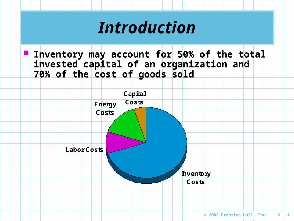
Inventory may account for 50% of the total invested capital of an organization and 70% of the cost of goods sold

Inventory Costs

Labor Costs

Energy Costs

Capital Costs


Introduction

All organizations have some type of inventory control system

Inventory planning helps determine what goods and/or services need to be produced

Inventory planning helps determine whether the organization produces the goods or services or whether they are purchased from another organization

Inventory planning also involves demand forecasting


The Inventory Process

Suppliers Customers

Finished Goods

Raw Materials

Work in Process

Fabrication/ Assembly

Inventory Storage

Inventory Processing


Controlling Inventory

Levels

Introduction

Forecasting Parts/Product

Demand

Planning on What Inventory to Stock

and How to Acquire It

Feedback Measurements to Revise Plans and

Forecasts

Figure 6.1

Inventory planning and control


Importance of Inventory Control

Five uses of inventory The decoupling function Storing resources Irregular supply and demand Quantity discounts Avoiding stockouts and shortages

The decoupling function Used as a buffer between stages in a

manufacturing process Reduces delays and improves efficiency



Storing resources Seasonal products may be stored to satisfy

off-season demand Materials can be stored as raw materials,

work-in-process, or finished goods Labor can be stored as a component of

partially completed subassemblies Irregular supply and demand

Demand and supply may not be constant over time

Inventory can be used to buffer the variability



Quantity discounts Lower prices may be available for larger orders Cost of item is reduced but storage and insurance

costs increase, as well as the chances for more spoilage, damage and theft.

Investing in inventory reduces the available funds for other projects

Avoiding stockouts and shortages Stockouts may result in lost sales Dissatisfied customers may choose to buy from

another supplier


Inventory Decisions

There are only two fundamental decisions in controlling inventory How much to order When to order

The major objective is to minimize total inventory costs

Common inventory costs are Cost of the items (purchase or material cost) Cost of ordering Cost of carrying, or holding, inventory Cost of stockouts


Inventory Cost Factors

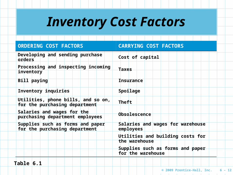
ORDERING COST FACTORS CARRYING COST FACTORS

Developing and sending purchase orders Cost of capital

Processing and inspecting incoming inventory Taxes

Bill paying Insurance

Inventory inquiries Spoilage

Utilities, phone bills, and so on, for the purchasing department Theft

Salaries and wages for the purchasing department employees Obsolescence

Supplies such as forms and paper for the purchasing department

Salaries and wages for warehouse employees

Utilities and building costs for the warehouse

Supplies such as forms and paper for the warehouse

Table 6.1


Inventory Cost Factors

Ordering costs are generally independent of order quantity Many involve personnel time The amount of work is the same no matter the

size of the order Carrying costs generally varies with the

amount of inventory, or the order size The labor, space, and other costs increase as

the order size increases Of course, the actual cost of items

purchased varies with the quantity purchased


Economic Order Quantity

The economic order quantityeconomic order quantity (EOQEOQ) model is one of the oldest and most commonly known inventory control techniques

It dates from a 1915 publication by Ford W. Harris

It is still used by a large number of organizations today

It is easy to use but has a number of important assumptions


Economic Order Quantity

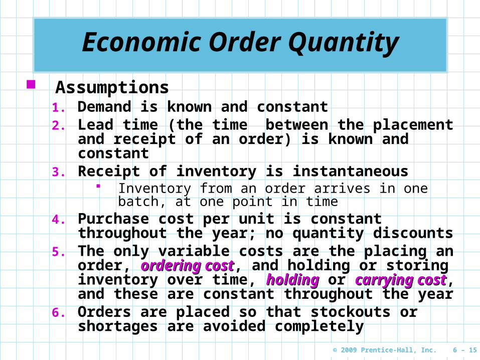
Assumptions1. Demand is known and constant2. Lead time (the time between the placement and

receipt of an order) is known and constant3. Receipt of inventory is instantaneous

Inventory from an order arrives in one batch, at one point in time

4. Purchase cost per unit is constant throughout the year; no quantity discounts

5. The only variable costs are the placing an order, ordering costordering cost, and holding or storing inventory over time, holdingholding or carrying costcarrying cost, and these are constant throughout the year

6. Orders are placed so that stockouts or shortages are avoided completely


Inventory Usage Over Time

Time

Inventory Level

Minimum Inventory

0

Order Quantity = Q = Maximum Inventory Level

Figure 6.2

Inventory usage has a sawtooth shape Inventory jumps from 0 to the maximum when the shipment arrives Because demand is constant over time, inventory drops at a uniform

rate over time


EOQ Inventory Costs The objective is to minimize total costs

The relevant costs are the ordering and carrying/holding costs, all other costs are constant. Thus, by minimizing the sum of the ordering and carrying costs, we are also minimizing the total costs

The annual ordering cost is the number of orders per year times the cost of placing each order

As the inventory level changes daily, use the average inventory level to determine annual holding or carrying cost The annual carrying cost equals the average inventory

times the inventory carrying cost per unit per year The maximum inventory is Q and the average inventory

is Q/2.


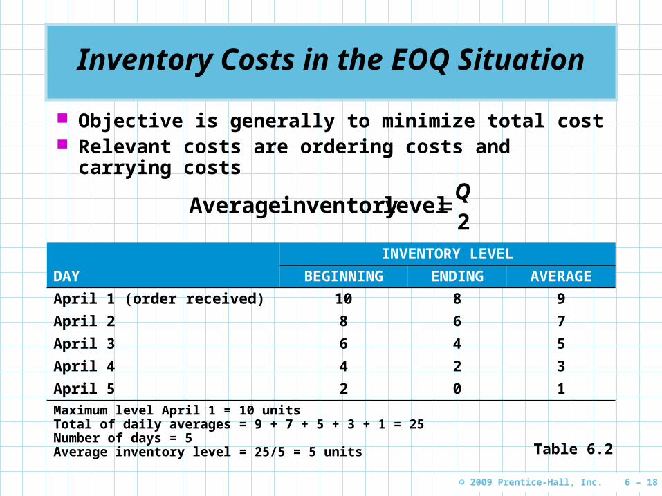
Inventory Costs in the EOQ Situation

Objective is generally to minimize total cost Relevant costs are ordering costs and carrying

costs

2level inventory Average

Q

INVENTORY LEVEL

DAY BEGINNING ENDING AVERAGE

April 1 (order received) 10 8 9

April 2 8 6 7

April 3 6 4 5

April 4 4 2 3

April 5 2 0 1

Maximum level April 1 = 10 unitsTotal of daily averages = 9 + 7 + 5 + 3 + 1 = 25Number of days = 5Average inventory level = 25/5 = 5 units Table 6.2



Develop an expression for the ordering cost.

Develop and expression for the carrying cost.

Set the ordering cost equal to the carrying cost.

Solve this equation for the optimal order quantity, Q*Q*.



Mathematical equations can be developed using

Q = number of pieces to orderEOQ = Q* = optimal number of pieces to order

D = annual demand in units for the inventory itemCo = ordering cost of each orderCh = holding or carrying cost per unit per year

Annual ordering cost Number of

orders placed per year

Ordering cost per

order

oCQD

orderper Cost orderper units ofNumber

Demand Annual



Mathematical equations can be developed using

Q = number of pieces to orderEOQ = Q* = optimal number of pieces to order

D = annual demand in units for the inventory itemCo = ordering cost of each orderCh = holding or carrying cost per unit per year

hCQ2

Annual holding cost Average

inventory

Carrying cost per unit

per year

Total Inventory Cost = ho CQ

CQ

D

2



Minimum Total Cost

Optimal Order Quantity

Curve of Total Cost Curve of Total Cost of Carrying of Carrying and Orderingand Ordering

Carrying Cost CurveCarrying Cost Curve

Ordering Cost CurveOrdering Cost Curve

Cost

Order Quantity

Figure 6.3

Optimal Order Quantity is when the Total Cost curve is at its lowest . This occurs when the Ordering Cost = Carrying Cost


Finding the EOQ

When the EOQ assumptions are met, total cost is minimized when Annual ordering cost = Annual holding cost

ho CQ

CQD

2

Solving for Q

ho CQDC 22

22Q

C

DC

h

o

*EOQ QQC

DC

h

o 2


Economic Order Quantity (EOQ) Model

hCQ2

cost holding Annual

oCQD

cost ordering Annual

h

o

C

DCQ

2 *EOQ

Summary of equations


Sumco Pump Company Example

Company sells pump housings to other companies

Would like to reduce inventory costs by finding optimal order quantity Annual demand = 1,000 units Ordering cost = $10 per order Average carrying cost per unit per year = $0.50

units 20000040500

10000122 ,

.))(,(*

h

o

C

DCQ



Total annual cost = Order cost + Holding cost

ho CQ

CQD

TC2

).()(,

502

20010

2000001

1005050 $$$



Program 6.1A



Program 6.1B


Purchase Cost of Inventory Items

Total inventory cost can be written to include the cost of purchased items

Given the EOQ assumptions, the annual purchase cost is constant at D C no matter the order policy C is the purchase cost per unit D is the annual demand in units

It may be useful to know the average dollar level of inventory

2level dollar Average

)(CQ


Purchase Cost of Inventory Items

Inventory carrying cost is often expressed as an annual percentage of the unit cost or price of the inventory

This requires a new variable

Annual inventory holding charge as a percentage of unit price or costI

The cost of storing inventory for one year is then

ICCh

thus,IC

DCQ o2

*


Sensitivity Analysis with the EOQ Model

The EOQ model assumes all values are know and fixed over time

Generally, however, the values are estimated or may change

Determining the effects of these changes is called sensitivity analysissensitivity analysis

Because of the square root in the formula, changes in the inputs result in relatively small changes in the order quantity

h

o

C

DC2EOQ


Sensitivity Analysis with the EOQ Model

In the Sumco example

units 200500

1000012

.))(,(

EOQ

If the ordering cost were increased four times from $10 to $40, the order quantity would only double

units 400500

4000012

.))(,(

EOQ

In general, the EOQ changes by the square root of a change to any of the inputs


Reorder Point:Determining When To Order

Once the order quantity is determined, the next decision is when to orderwhen to order

The time between placing an order and its receipt is called the lead timelead time (LL) or delivery delivery timetime Inventory must be available during this period to

met the demand When to order is generally expressed as a

reorder pointreorder point (ROPROP) – the inventory level at which an order should be placed

Demand per day

Lead time for a new order in daysROP

d L


Determining the Reorder Point

The slope of the graph is the daily inventory usage Expressed in units demanded per day, d

If an order is placed when the inventory level reaches the ROP, the new inventory arrives at the same instant the inventory is reaching 0


Procomp’s Computer Chip Example

Demand for the computer chip is 8,000 per year Daily demand is 40 units Delivery takes three working days

ROP d L 40 units per day 3 days 120 units

An order is placed when the inventory reaches 120 units

The order arrives 3 days later just as the inventory is depleted


The Reorder Point (ROP) Curve In

vent

ory

Lev

el (

Uni

ts)

Q*

ROP(Units)

Slope = Units/Day = d

Lead Time (Days) L


EOQ Without The Instantaneous Receipt Assumption

When inventory accumulates over time, the instantaneous receiptinstantaneous receipt assumption does not apply

Daily demand rate must be taken into account The revised model is often called the production production

run modelrun model

Inventory Level

Time

Part of Inventory Cycle Part of Inventory Cycle During Which Production is During Which Production is Taking PlaceTaking Place

There is No Production There is No Production During This Part of the During This Part of the Inventory CycleInventory Cycle

t

Maximum Inventory

Figure 6.5


EOQ Without The Instantaneous Receipt Assumption

Instead of an ordering cost, there will be a setup cost – the cost of setting up the production facility to manufacture the desired product Includes the salaries and wages of employees

who are responsible for setting up the equipment, engineering and design costs of making the setup, paperwork, supplies, utilities, etc.

The optimal production quantity is derived by setting setup costs equal to holding or carrying costs and solving for the order quantity


Annual Carrying Cost for Production Run Model

In production runs, setup costsetup cost replaces ordering cost

The model uses the following variables

Q number of pieces per order, or production run

Cs setup cost

Ch holding or carrying cost per unit per yearp daily production rated daily demand ratet length of production run in days



Maximum inventory level (Total produced during the production run) – (Total used during the production run)

(Daily production rate)(Number of days production)– (Daily demand)(Number of days production)

(pt) – (dt)

since Total produced Q pt

we knowpQ

t

Maximum inventory

level

pd

QpQ

dpQ

pdtpt 1



Since the average inventory is one-half the maximum

pdQ

12

inventory Average

and

hCpdQ

1

2cost holding Annual


Annual Setup Cost for Production Run Model

sCQD

cost setup Annual

Setup cost replaces ordering cost when a product is produced over time (independent of the size of the order and the size of the production run)

and

oCQD

cost ordering Annual


Determining the Optimal Production Quantity

By setting setup costs equal to holding costs, we can solve for the optimal order quantity

Annual holding cost Annual setup cost

sh CQD

CpdQ

1

2

Solving for Q, we get

pd

C

DCQ

h

s

1

2*


Production Run Model

Summary of equations

pd

C

DCQ

h

s

1

2 quantity production Optimal *

sCQD

cost setup Annual

hCpdQ

1

2cost holding Annual

If the situation does not involve production but receipt of inventory over a period of time, use the same model but replace CCss with CCoo


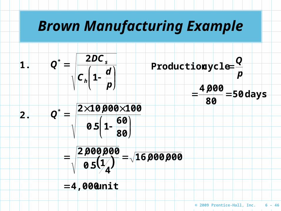
Brown Manufacturing Example

Brown Manufacturing produces commercial refrigeration units in batches

Annual demand D 10,000 units

Setup cost Cs $100

Carrying cost Ch $0.50 per unit per yearDaily production rate p 80 units daily

Daily demand rate d 60 units daily

How many refrigeration units should Brown produce in each batch?How long should the production cycle last?



pd

C

DCQ

h

s

1

2*1.

2.

8060

150

100000102

.

,*Q

00000016

4150

0000002,,

.

,,

units 4,000

days 50800004

,

pQ

cycle Production



Program 6.2A



Program 6.2B


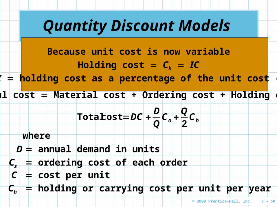
Quantity Discount Models

Quantity discounts are commonly available The basic EOQ model is adjusted by adding in the

purchase or materials cost

Total cost Material cost + Ordering cost + Holding cost

ho CQ

CQD

DC2

cost Total

where

D annual demand in units

Cs ordering cost of each orderC cost per unit

Ch holding or carrying cost per unit per year



Quantity discounts are commonly available The basic EOQ model is adjusted by adding in the

purchase or materials cost

Total cost Material cost + Ordering cost + Holding cost

ho CQ

CQD

DC2

cost Total

where

D annual demand in units

Cs ordering cost of each orderC cost per unit

Ch holding or carrying cost per unit per year

Holding cost Ch IC

I holding cost as a percentage of the unit cost (C)

Because unit cost is now variable



A typical quantity discount schedule

DISCOUNT NUMBER

DISCOUNT QUANTITY DISCOUNT (%)

DISCOUNT COST ($)

1 0 to 999 0 5.00

2 1,000 to 1,999 4 4.80

3 2,000 and over 5 4.75

Table 6.3

Buying at the lowest unit cost is not always the best choice



Total cost curve for the quantity discount model

Figure 6.6

TC Curve for Discount 1

TC Curve for Discount 3Total Cost

$

Order Quantity

0 1,000 2,000

TC Curve for Discount 2

EOQ for Discount 2


Brass Department Store Example

Brass Department Store stocks toy race cars Their supplier has given them the quantity

discount schedule shown in Table 6.3 Annual demand is 5,000 cars, ordering cost is $49, and

holding cost is 20% of the cost of the car The first step is to compute EOQ values for each

discount

order per cars 70000520

49000521

).)(.())(,)((

EOQ


49000522

).)(.())(,)((

EOQ


49000523

).)(.())(,)((

EOQ



The second step is adjust quantities below the allowable discount range

The EOQ for discount 1 is allowable The EOQs for discounts 2 and 3 are outside the

allowable range and have to be adjusted to the smallest quantity possible to purchase and receive the discount

Q1 700

Q2 1,000

Q3 2,000



The third step is to compute the total cost for each quantity

DISCOUNT NUMBER

UNIT PRICE

(C)

ORDER QUANTITY

(Q)

ANNUAL MATERIAL COST ($)

= DC

ANNUAL ORDERING COST ($) = (D/Q)Co

ANNUAL CARRYING COST ($) = (Q/2)Ch TOTAL ($)

1 $5.00 700 25,000 350.00 350.00 25,700.00

2 4.80 1,000 24,000 245.00 480.00 24,725.00

3 4.75 2,000 23,750 122.50 950.00 24,822.50

The fourth step is to choose the alternative with the lowest total cost

Table 6.4



Program 6.3A



Program 6.3B


Use of Safety Stock

If demand or the lead time are uncertain, the exact ROP will not be known with certainty

To prevent stockoutsstockouts, it is necessary to carry extra inventory called safety stocksafety stock

Safety stock can prevent stockouts when demand is unusually high

Safety stock can be implemented by adjusting the ROP


Use of Safety Stock

The basic ROP equation is

ROP d Ld daily demand (or average daily demand)L order lead time or the number of working days it takes to deliver an order (or average lead time)

A safety stock variable is added to the equation to accommodate uncertain demand during lead time

ROP d L + SSwhere

SS safety stock


Use of Safety Stock

StockoutStockoutFigure 6.7(a)

Inventory on Hand

Time


Use of Safety Stock

Figure 6.7(b)

Inventory on Hand

Time

Stockout is AvoidedStockout is Avoided

Safety Safety Stock, Stock, SSSS

Date post:	15-Dec-2015
Category:	Documents
Upload:	fred-douthit
View:	223 times
Download:	5 times

© 2008 Prentice-Hall, Inc. Chapter 6 To accompany Quantitative Analysis for Management, Tenth...

Documents