+ All Categories
Home > Documents > , Holger Neubert , Rolf Disselnkötter Transient Finite ... - COMSOL … · 2011-03-08 ·...

, Holger Neubert , Rolf Disselnkötter Transient Finite ... - COMSOL … · 2011-03-08 ·...

Date post: 07-Apr-2020
Category:
Upload: others
View: 10 times
Download: 1 times
Share this document with a friend
18
Transient Finite Element Analysis Thomas Bödrich 1 , Holger Neubert 1 , Rolf Disselnkötter 2 2010-11-17 | Slide 1 Transient Finite Element Analysis of a Spice-Coupled Transformer with COMSOL-Multiphysics 1) TU Dresden, Institute of Electromechanical and Electronic Design 2) ABB AG, Corporate Research Center, Germany Presented at the COMSOL Conference 2010 Paris
Transcript

Transient Finite Element Analysis Thomas Bödrich1, Holger Neubert1, Rolf Disselnkötter2

���2010-11-17 | Slide 1

Transient Finite Element Analysis of a Spice-Coupled Transformer with COMSOL-Multiphysics

1) TU Dresden, Institute of Electromechanical and Electronic Design2) ABB AG, Corporate Research Center, Germany

Presented at the COMSOL Conference 2010 Paris

Outline

Introduction

Transformer Modelling

� Magnetic test model

� Coupling with Spice

� Settings

Results

� Transient signals

� Flux density distribution

���

� Flux density distribution

� Stray fields

Conclusions

Outlook

2010-11-17 | Slide 2

IntroductionModelling of Passive and Active Current Transformers

Purpose:

Support the design process by predicting the influences ofpredicting the influences of

� nonlinearities of the magnetization curve (initial permeability, saturation, …)

� special core and winding geometries (air gaps, partial windings, asymmetries, …)

� external and internal stray fields

� eddy currents (both in the core and in the windings)

���

in the windings)

� magnetic hysteresis

� coupling to electric circuits (transient response)

� thermal effects

in large current and frequency operating ranges

2010-11-17 | Slide 3

Challenges with FE-Modelling

Combination of requirements:

� 3D geometry (potentially with low symmetry)

� Scale range typically > 100:1 (e.g. air gap / transformer size)

� Magnetic material with (strongly) nonlinear characteristic

� Presence of both injected and induced currents

� Coupling to electric circuits (may be nonlinear as well)

� Transient analysis required

� Modelling of eddy currents (suited mesh required)

���

� Modelling of eddy currents (suited mesh required)

� Modelling of magnetic hysteresis

� Bidirectional thermal coupling

� Numerical stability in wide amplitude and frequency ranges

© ABBOct. 21, 2010 | Slide 4

Simulation with COMSOL MultiphysicsTest Model

� Square-shaped magnetic core frame with central hole of 3.5 cm width and two of 3.5 cm width and two

different types of air gaps (full and partial)

� Bus-bar type bulk primary

Cu-conductor (N1 = 1)

� Secondary winding (N2 = 1000) split into two

linear box-shaped sections

���2010-11-17 | Slide 5

linear box-shaped sections

� Boundary condition “Magnetic insulation” on

outer cylinder surfaces

Magnetic CoreMaterial Characteristic

� FeSi3-type magnetic material (M90-23P; µmax ≈ 50,000)

� Nonlinear characteristic

� Extrapolation with µr diff = 1 up to very high fields for a stable convergence of the solution

� Transient 3D quasi-static magnetic problem: induction

currents mode (emqa: vector potential A is dependent variable)

���

potential A is dependent variable)

� � H = f(|B|)eB

(table in the materials/coefficients library)

2010-11-17 | Slide 6

Secondary WindingCurrent Distribution

� Winding sections composed of 2 x 4 prismatic elements

Secondary current implemented as � Secondary current implemented as

a locally constant external current density:

� Continuity preserved at the 45°

interfaces of the prismatic elements

iie

A

tiNt eJ ⋅=

sec

22

)()(

���

� Injection of a locally constant primary external current density

2010-11-17 | Slide 7

z

e

A

tit eJ ⋅=

prim

11

)()(

Secondary Winding Calculation of the Output Voltage

� Ek: amplitude of the electric field component in the direction of the current

i2coilsec ViRV −⋅=

∑8

N direction of the current

density in kth domain (i.e., Ek = Ex_emqa or Ek = Ez_emqa)

� Calculation of Kk implemen-ted by defining Ex_emqa and Ek = Ez_emqa as

integration coupling varia-bles in the respective

(k = 1, 2, …, 8)

∑∫=

⋅==

8

1sec

i dk

k

l

ΚA

NV lE

dVEΚ

kV

kk ∫=

���

bles in the respective subdomains.

2010-11-17 | Slide 8

Electric CircuitCoupling to a Spice Model

� I1source 0 1 sin(0 1000 50)

� RprimExt 1 2 1RprimExt 1 2 1

� X1 2 0 primFEM

� X2 3 0 secFEM

� RsecExt 3 0 1

� .SUBCKT primFEM Vprim i1 COMSOL: *

� .ENDS

� .SUBCKT secFEM Vsec i2 COMSOL: *

� Currents and voltages of the FE-model are linked to the primary and secondary electric circuits

���

� .SUBCKT secFEM Vsec i2 COMSOL: *

� .ENDS

� .END

2010-11-17 | Slide 9

secondary electric circuits

� Transformer here operated in passive mode (without electronic feedback)

� More complex circuit model could be used as an alternative

Settings

� Coarse mesh with element type “Vector–Linear”

� 14613 degrees of freedom

� Solver: Time dependent

� Time range: 60 ms

(3 signal periods)

� Linear system solver: Direct (3.5: PARDISO,

4.0: MUMPS, PARDISO,

���

4.0: MUMPS, PARDISO, SPOOLES)

� Solution time: 210 … 440 s*

(PC with Intel Core2 Quad CPU 2.40 GHz, 8 GB RAM)

*) dep. on tolerance settings

© ABBOct. 21, 2010 | Slide 10

Results of the Transient SimulationsPrimary and Secondary Currents

� Primary current(1000 A, 50 Hz)

� Resulting secondary

current of a “bad” current transformer (1:1000)

���

transformer (1:1000) showing

� Initial transient response

� Current error

� Phase shift

2010-11-17 | Slide 11

Instantaneous Flux Density Distribution

� Influence of demagnetizing fields from the full air gap (top) and the secondary (top) and the secondary

windings at i1(t) = i1,max

� Snap-shot at i1(t) = 0 with

still high induction level close to the partial gap

���

close to the partial gap (right) resulting from the phase shift of secondary

current

(B: absolute value)

2010-11-17 | Slide 12

Influence of Stray Fields

���

� Even at times when the magnetization current is zero there may be still high local induction levels due to stray fields from the air gaps.

� Stray fields may cause bandwidth limitations and local losses

© ABBOct. 21, 2010 | Slide 13

Stray Field Distribution

� Stray field distribution at zero magnetization current

� Stray field distribution at maximum primary current

���© ABBOct. 21, 2010 | Slide 14

ConclusionsExperiences with 3D Transient Magnetic Simulations

� 3D transient FEA with COMSOL and Spice coupling is helpful in the design and for a better understanding of electro-magnetic systems which exhibitelectro-magnetic systems which exhibit

� more complex core and winding geometries

� magnetic components with nonlinear materials

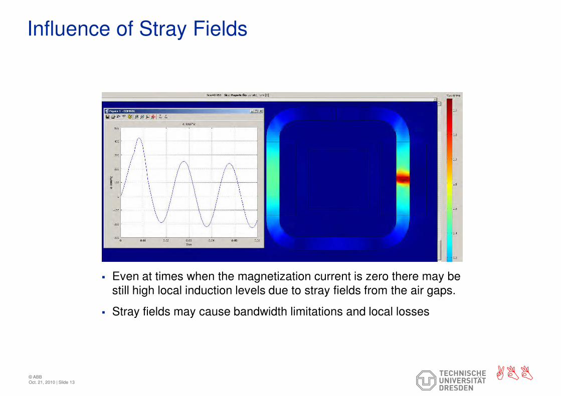
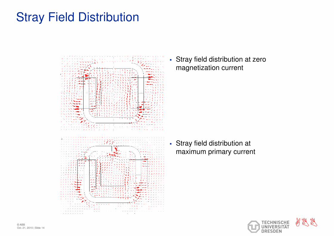
� coupling to external and internal stray fields

� coupling to electric circuits

� Going from 2D to 3D modelling can be tricky, especially if combined with

���

combined with

� nonlinearities

� a large scale range

� transient analysis

2010-11-17 | Slide 15

Conclusions IIExperiences with 3D Transient Magnetic Simulations

In order to obtain

� numerical stability and fast convergence of the solution

� broad accessible operation ranges (up to magnetic saturation and high frequencies)

� numerical robustness with respect to geometry and

material variation

care has to be taken with respect to

� geometry modelling (avoid curved faces and too many details)

���

details)

� meshing and element type (avoid inverted elements

and high number of DOF)

� solver selection and settings

2010-11-17 | Slide 16

OutlookPlanned Improvements

� Numerical stability in extended parameter ranges

� Consideration of eddy current effects (currently suppressed)

Electrical circuits with higher complexity (e.g. electronic � Electrical circuits with higher complexity (e.g. electronic feedback)

� Thermal coupling

���2010-11-17 | Slide 17

Thank You!

� Questions?

���© ABBOct. 21, 2010 | Slide 18


Recommended