81
7 AD-A103 724 TRANSPOKTATION SYSTEMS CENTER LAMBNIDGL MA F/A 20/11 HEL COPER NOIT S ANALYSI8 - ROUN -ARBIN LSAEl L U LASSIFIED TSC-FAA-Al-11 FAA-ACE-RI11 NL mh//////I//I/l ""-IIIIII""
| Date post: | 14-May-2018 |
| Category: |
Documents |
| Upload: | nguyenthuy |
| View: | 214 times |
| Download: | 1 times |

7 AD-A103 724 TRANSPOKTATION SYSTEMS CENTER LAMBNIDGL MA F/A 20/11HEL COPER NOIT S ANALYSI8 - ROUN -ARBIN
LSAEl L
U LASSIFIED TSC-FAA-Al-11 FAA-ACE-RI11 NL
mh//////I//I/l
""-IIIIII""

REPORT NO. FAA-EE-81-13 LEVELICHELICOPTER NOISE ANALYSIS --
ROUND-ROBIN TEST
E. J. Rickley
U.S. DEPARTMENT OF TRANSPORTATIONRESEARCH AND SPECIAL PROGRAMS ADMINISTRATION
Transportation Systems CenterCambridge MA 02142
DTIC
AUGUST 1981FINAL REPORT
DOCUMENT IS AVAILASLE TO THE PUSLICTHROUGH THE NATIONA,.. TECHNICALINFORMATION SERVICE. SPRINGFIELD.VIRGINIA 221St:
8
LU.
Prepared forUS, DEPARTMENT OF TRANSPORTATIONFEDERAL AVIATION ADMINISTRATION
Office of Environment and EnergyWashington DC 20591
81 9 03 09 6 ..
INORATO SEVCLIGFED

NOTICE
This document is disseminated under the sponsorshipof the Department of Transportation in the interestof information exchange. The United States Govern-ment assumes no liability for its contents or usethereof.
NOTICE
The United States Government does not endorse pro- V
ducts or manufacturers. Trade or manufacturers'names appear herein solely because they are con-sidered essential to the object of this report.
7
V
..... _ _ __ _ __ __ _ __ __,_ __ __ _ __ _ __
am m m m- | | -

Technical Reoport Documentation Page
_1. -it"" Me.- 2. Goemment Accession No. 3. Recipet's Catalog N.
__ FAA-aEE 813
4. itle end Subtitle
HELICOPTER NOISE ANALYSIS R-_OUND-ROBIN TESiTS
8. Perforuming Orguanisation eport Me.
EdwardJ./Rickleyj ___________
9. Performing Orson. set ei m* nd Adds...e 10. Work Unit No. (TRAISIU.S. Department of Transportation FA153/R1102Research and Special Programs Administration 1.cet orev6etN.Transportation Systems Center _____________
Cambridge MA 02142 3....eetidCuid12. Sponsoring Agency Nae.. end AddressU.S. Department of Transportation FinallKepwt'Federal Aviation Administration Jan..-439tO ay 181,1Office of Environment and Energy 4 imprln,*"earWashington DC 20591 AEE-120 -
Is. Supplementary Notes
16. Abstract
-,;,his report documents the results of an international Round RobinTest on the analysis of helicopter noise. Digital spectral noisedata of a 3.5-second simulated helicopter flyover and identicalanalog test tapes containing helicopter noise data, referencesignals, test tones and time code signals were sent to 13participating organizations. The purpose of the test was toevaluate data reduction systems and procedures; to determine themagnitude of the variability between representative systems andorganizations; and to identify potential causes and assist inestablishing recommended procedures designed to minimize thevariability.
17. Key Werds Is. Distribution Staemeuent
Acoustic, Helicopter Noise, DOCUMENT I SAVAILABLE 10 THE PUBLICAircraft Noise, Noise Analysis THPIO4TENATNIONAL TCHNICAL
VIRGINIA 22161
It. btouly Classic (of this foew) 3D. Somirity Ciossed. EoE'two poe) 21. NMe oPages 2.Ps.
Unclassified Unclassified 82 2
Per. DOT F 1700.7 a3-72) noedclf of complete I"* owhrl

I7
PREFACE
A round-robin test was conducted to promote uniformity in the
analysis of data for describing helicopter noise for international
helicopter certification standards. Identical analog tape record-
ings containing helicopter noise data, and reference and test sig-nals were sent to 13 acoustic-analysis laboratories around
the world. Seven of the 13 organizations responded and
supplied test data reduced from the tapes. These data plus the
TSC data are tabulated and discussed in this report. Data from
three additional organizations, which were received late, are
tabulated in the report without comment. Since this was a com-
pletely voluntary test, the time and effort of the respondents are
acknowledged with appreciation.
The following members of the Noise Measurement and Assessment
Laboratory of the Transportation Systems Center contributed to the
preparation of this report: A. Dahlgren, A. DiTomaso, J. Hickey,
R. Quinn and N. Rice.
Aocession For
NTIS GPA&I
DTIC TAB
Just if i t; t] n :
By . ..
itv CodesDi f i, Id/or
iii

fill
IIJ
S S
ANS

TABLE OF CONTENTS
Section Page
1. INTRODUCTION ......................................... 1
2. GENERAL .............................................. 3
3. EXPERIMENTAL APPROACH .............................. 5
3.1 Analog Tape Recording ......................... 53.2 Digital Tabulations One-Third Octave Spectra.. 83.3 Instructions .................................... 9
4. RESULTS ............................................. 11
4.1 Summary Respondent Information ................ 114.2 System Frequency Response ..................... 134.3 Linearity Test ................................. 134.4 Detector Transient Response ................... 154.5 Helicopter Noise Data--Test Run 11, 12, 13, 14 184.6 Digital Data ................................... 304.7 Atmospheric/Distance Corrections .............. 33
S CONCLUSIONS ......................................... 36
APPENDIX A TEST PROCEDURE AND SAMPLE DATA-REPORTING SHEETS ............................ A-1
REFERENCES ................................................ R-1
vf
V
-- --- ~ ~ ... -- ---- ~ .- -- -- - - -__ ~ --- ~- ~-,

LIST OF ILLUSTRATIONS
Figure Page
1. System Linearity Test at 1 kHz .................... 14
2. Detector Transient Response ....................... 16
3. Summary Data, Run No. 11 - Approach Centerline .... 24
4. Summary Data, Run No. 12 - Takeoff Centerline ..... 25
S. Summary Data, Run No. 13 - Flyover Centerline ..... 26
6. Summary Data, Run No. 14 - Flypast Centerline ..... 27
vi

LIST OF TABLES
Table Page
1. RESPONDENT SUMMARY INFORMATION ................... 12
2. ANALYSIS SUMMARY, RUN NO. 11 - APPROACHCENTERLINE ......................................... 19
3. ANALYSIS SUMMARY, RUN NO. 12 - TAKEOFFCENTERLINE ......................................... 20
4. ANALYSIS SUMMARY, RUN NO. 13 - FLYOVERCENTERLINE ......................................... 21
5. ANALYSIS SUMMARY, RUN NO. 14 - FLYPASTCENTERLINE ......................................... 22
6. DIGITAL DATA SUMMARY ............................... 32
7. ATMOSPHERIC/DISTANCE CORRECTIONS, 10-METERPROCEDURE .......................................... 34
8. ATMOSPHERIC/DISTANCE CORRECTIONS, LAYEREDPROCEDURE .......................................... 35
vii/viii

SUMMARY
The results of an international Round-Robin Test on the Analy-
sis of Helicopter Noise data are reported. Seven of thirteen
participating organizations, who received identical copies of
a test tape containing calibration signals, reference signals,and noise data from four helicopter flyover operations, respon-
ded by returning processed results from the test tape using in-
structions and procedures provided. As part of the test, digi-
tal tabulations for 3.5 seconds of a simulated helicopter fly-
over were also provided in an attempt to isolate computational
or procedural variations between participants. To preserve
anonymity of the participants no means is provided to identify
respondents.
The results of the computations on the digital data showed
good procedural application of the Annex 16 methodology for
computation of noise indexes, such as PNL and PNLT. In addition,
calculated adjustments for distance and meteorological conditions
were in excellent agreement.
The results of the reductions and analyses of the analog
tape showed an exceptionally small within-organization variability
(standard deviation of 0.2 dB or less for the measured noise
indexes). The organization-to-organization variability was 0.5 dB
or less. A variability of 0.7 dB or less was achieved for the
test run No. 13 (level helicopter flyover) which contained signals
with the most rapid transient changes.
Although the data set for this test was small (eight organiza-
tions, including TSC), a grouping of the data could be seen. A
close grouping (variability 0.2 dB) was formed from data by re-
spondents who used instrumentation from a single manufacturer and
external computer averaging with an effective RC time constant of
750 milliseconds. A second group (variability 0.5 dB) was formed
by respondents who used commercially packaged systems of two
manufacturers (3 types of equipment) set to an effective RC time
ix
, . I n I I -
constant of 1000 milliseconds. Data from three additional organ-
izations, which were received late, have been included in the
tables and figures of the report without comment. I
/
, I
9
x

1. INTRODUCTION
At the October 1979 meeting of the International Civil Avia-
tion Organization, Committee on Aircraft Noise (ICAO/CAN), Working
Group B, it was proposed that a round-robin test be conducted to
promote uniformity in the analysis of data for describing heli-
copter noise for international helicopter certification standards.
The U.S. DOT/Transportation Systems Center (TSC) Kendall
Square, Cambridge, MA was requested by the Federal Aviation Admin-
istration/Office of Energy and Environment, who sponsored the
test, to act as the focal point for the definition of the test
procedure, and for the subsequent collection and evaluation of re-
sults generated by the nations and organizations participating.
Accordingly, TSC generated seventeen identical helicopter-noise
test-recordings, identified procedures for their reduction, and
distributed them to thirteen acoustic analysis laboratories
around the world. Seven out of the thirteen organizations re-
sponded by returning test data reduced from the tapes. Since
labor and materials for this test were supplied voluntarily,
the efforts are acknowledged with appreciation.
Test tapes and procedures were sent to the following:
The de Havilland Aircraft of Canada Ltd.
Downsview, Ontario
Direction des Transports AerieaneParis, France
Societe Nationale Industrielle Aerospatiale
Marignane, France
Federal Ministry of TransportCivil Aviation Department
Federal Republic of Germany
Costruzioni Aeronautiche
Giovanni Agusta
Gallarate, Italy (two tapes)
m m m1

Kawasaki Heavy Industries, Ltd
Aircraft Manufacturing Division
GIFU, Japan
Department of Industry
London, England
Westland Helicopters
United Kingdom
Bell Helicopter Company
Fort Worth, Texas
Boeing-Vertol Company
Philadelphia, Pa. (two tapes)
FAA Noise Monitoring Lab
Washington, D.C.
Sikorsky Aircraft
Stratford, Connecticut (two tapes)
Commission USSR for ICAO
Moscow, USSR.
In order to preserve anonymity, the eight participants are not
identified, nor does the reference number assigned reflect the
above ordering.
Note: Three additional organizations responded late, their data
are included in the figures and tabulations of this reportwithout comment.
2

2. GENERAL
The complexity of helicopter flyby noise, which contains non-stationary random noise, fluctuating periodic signals and impul-
sive signals, in combination with a variety of noise measurementand data processing systems and procedures could result in avariation of derived flyby noise levels and descriptors measuredfor the same type aircraft. The purpose of this round-robin testis to evaluate data reduction systems and procedures to determinethe magnitude of the variability among representative systemsand organizations, and to identify potential causes, and thereforeassist in establishing recommended procedures designed to minimizethe variabilty.
As part of the evaluation, an analog test tape was generatedcontaining helicopter noise data, reference signals, test tonesand time-code signals. Seventeen copies of tape recordings were
carefully made for distribution to the round-robin test partici-
pants. Prior to shipment, each tape was processed and analyzedusing the TSC analysis system to insure uniformity of the data oneach tape.
The participants were requested to process the data from thetapes using the instructions provided and the procedures outlinedin the ICAO International Standards and Recommended Practices onAircraft Noise, Annex 16, Third Edition, July 1978 (Reference 1).At present Annex 16 does not apply to helicopters but will when therecommendations of CAN 6 for helicopter standards are incorporatedas an amendment. The procedures of the Third Edition supplementedby the appropriate CAN 6 recommendations were to be used in this
test as specified in the supplied test instructions. (Appendix A)
Digital tabulations of one-third octave sound pressurelevels for seven consecutive 0.5-second periods around PNLTM fora simulated helicopter flyover were also provided for evaluationin an attempt to isolate possible computational or proceduralvariations between participants, and to evaluate the techniques
--
--
---

used to apply atmospheric and distance corrections to the data.
The data submitted by eight respondents (including TSC) iz
summarized and tabulated in this report. To preserve anonymity
of the respondents, no means is provided to identify participants
from the numeric code used in summarizing data.
4

3. EXPERIMENTAL APPROACH
Each participant in the test was provided with:
1) A test tape recording consisting of calibration and
reference signals and noise data from three heli-
copter flyovers and one helicopter flypast.
2) Digital tabulations of one-third-octave-band sound-
pressure levels of seven consecutive 0.5-second in-
crements around PNLTM for a simulated flyover.
3) A set of instructions and standard data reporting
forms. (Appendix A)
3.1 ANALOG TAPE RECORDING
A maste6 analog test tape recording was generated on a two-
track NAGR-A IVSJ recorder with a Cue Track at a speed of 7-1/2
inches per second. Seventeen identical copies were made also
using NAGRA IVSJ recorders operating at 7-1/2 inches per second
in the copying process.
To insure that all copies were identical, each tape was re-
duced on the TSC analysis system (GenRad 1921) before distribution
to the participant. The reduced data were stored on computer disc
for further evaluation if the need arose. A tape was rejected if
a variation in either OASPL, PNL, PNLT, EPNL was found to be
greater than 0.1 dB from the average of all tapes.
The contents of the test tape are summarized below.
Time Code
Test Run Data: (Channels 1 & 2 (Cue Track)
I Playback Reference Tone, 1000 Hz
2 Frequency Response Signal, Pink Noise 00:02:04.0
3 Amplitude Calibration, 250 Hz, 94 dB 00:03:20.0
4 Amplitude Calibration, 500 Hz, 94 dB 00:04:21.0
5 Amplitude Calibration, 1000 Hz, 94 dB 00:05:39.0
S
--

Time Code
Test Run Data: (Channel 1 & 2) (Cue Track)
6 Linearity Test Tone, 1000 Hz, 84 dB 00:06:56.0
7 Linearity Test Tone, 1000 Hz, 74 dB 00:08:16.0
8 Linearity Test Tone, 1000 Hz, 64 dB 00:09:32.0
9 Linearity Test Tone, 1000 Hz, 54 dB 00:10:50.0
10 Detector Test, 1000 Hz tone bursts 00:12:25.0
11 Helicopter Flyover, Approach centerline 00:14:50.0
12 Helicopter Flyover, Takeoff centerline 00:15:42.0
13 Helicopter Flyover, Level Flightcenterline 00:16:40.0
14 Helicopter Flypast, Level Flight
sideline 00:17:31.0
5 Playback Reference Tone, 1000 Hz0
Note: Channel 1 and 2 contain identical data.
3.1.1 Reference Tones
The signals of test runs 1 and 15 were to be used to adjust
the electronics of the reproduce/analysis systems to full scale,
thus insuring that the test signal would not overload the ampli-
fiers in the analysis system. A measurement of the frequency of
these signals by the respondents provides a measure of the accuracy
of the speed of the tape recorder used to reproduce the data.
3.1.2 Pink Noise
A pink noise signal, provided in test run 2, was to be used
to correct for the spectral irregularities of the respondents'
reproduce/analysis systems. Twenty seconds of pink noise data
were to be energy averaged and referenced back to the frequency
band of the chosen amplitude reference tone.
6

3.1.3 Calibration Signals
Absolute calibration of the analysis system was provided
through the use of the 250-, 500-, or 1000-Hz amplitude ref-
erence tone, test runs 3, 4, and 5. A respondent could use
the calibration frequency of his choice with the stipulation that
the spectral corrections should be referenced back to the parti-
cular frequency band of the reference tone.
3.1.4 Linearity Test Tones
The l-kHz tones of runs 6, 7, 8,and 9 in conjunction with
that of test run 5, provided a measure of the linearity of the
respondent's reproduce/analysis systems at 1 kHz, and at four
levels over the upper 40 dB of the system's dynamic range. Sys-
tems with a single detector would be checked at 1 kHz while only
the detector in the l-kHz band would be checked on systems with
multiple detectors.
3.1.5 Detector Dynamics
Test run 10 consists of a constant-level l-kHz tone followed
by l-kHz tone bursts which were to be used to obtain the dynamic
detector characteristics of the respondent's analysis system at
1 kHz. Tone bursts in lengths of 1/4, 1/2, and 2 seconds were
provided, five each.
The start of each pulse was staggered in time (i.e., 100 msec
was added to the start of consecutive pulses) such that when
the test sequence was started as prescribed, an appropriate
alignment would be assured for at least one pulse in those systems
whose detector mode of operation used a 0.5-second integration
time followed by computer smoothing. The resulting measured
levels could then be used to assess the dynamic rise and fall
characteristics of the detectors in all systems. This was not
an all inclusive test but would provide a good measure of the
detector characteristics.
7
_ _ .- '. ' . .... . _ _ .' ,,4

3.1.6 Helicopter Noise Data
Noise data from helicopter approach, take-off and level fly-
over and level flypast were selected for inclusion in this test.
These events were selected to include impulsive noise (blade slap),
pure tones, band-sharing, broadband noise and psuedotones. The
original recordings were made with the microphone at 1.2 meters
over grass and located as follows:
Run 11, (Approach) directly under the approach flight path.
(10-dB-down duration, 16.5 seconds)
Run 12, (Takeoff) directly under the takeoff flight path.
(10-dB-down duration, 9.5 seconds)
Run 13, (Level Flyover) directly under the flight path.
(10-dB-down duration 6.0 seconds)
Run 14, (Level Flypast) 150 meters to the side of the flight
path. (10-dB-down duration, 17.0 seconds)
Because of the wide dynamic range of the spectral levels,
of helicopter noise, and the limitation in dynamic range charac-
teristics of present day tape recorders, it was necessary to
"shape" the low frequencies of the helicopter noise, to insure that
the complete flyover noise history could be recorded on a single
recorder channel unaffected by the electronic noise-floor of the
record/reproduce recorders. No instructions were given to the
participants to correct for this shaping, nor was it necessary
because all participants would be working with the same "shaped"
spectra.
3.2 DIGITAL TABULATIONS ONE-THIRD OCTAVE SPECTRA
One-third octave digital sound pressure level data of a
simulated flyover for seven consecutive 0.5-second periods around
PNLTM was supplied. Participants were instructed to calculate
indexes from these spectra using the same computer processing
technique which was used for the analog tapes. These results
would provide an insight into possible variations in final re-
sults between respondents because of calculation, procedural
8
V

differences, or even computer roundoff techniques.
in addition, methodology for correcting data for atmospheric
absorption by both the "10-meter" and "layered" technique would be
compared. A flight-path profile and temperature/humidity-data-
versus-altitude were supplied (see Appendix A, Figure 4.1 and
Table 4.2 ), with instructions to adjust the PNLTM spectra for
positional and meteorological correction by both the "10-meter"
and "layered" procedures.
The equations of SAE-ARP-866A (3/15/75) were to be used for
computing the atmospheric absorption corrections. The data was
to be corrected back to the reference meteorological condition of
Annex 16 (25°C and 70% relative humidity).
The "ten-meter" procedure assumes constant temperature/humi-
dity conditions versus altitude, based on meteorological measure-
ment made 10 meters above the ground. Although not specified, a
microphone height of 0.0 feet (flush or ground level) was to be
assumed with the aircraft in level flight.
The following steps were to be used for the layered procedure:
a) Divide the sound-propagation path into increments of
30 meters in altitude.
b) Determine the average temperature and relative humidity
in each 30-meter altitude increment.
c) Calculate the atmospheric-attenuation rate in each one-
third-octave band in each altitude increment.
d) The mean atmospheric-attentuation rate over the complete
propagation path for each one-third-octave band must be
computed and used to calculate the corrections required.
3.3 INSTRUCTIONS
A set of instructions, which take into account the latest
proposed changes to Annex 16,were provided (See Appendix A).
It was requested that deviation from the procedures be minimized,
and where absolutely necessary a description of the deviation be
9

supplied. Standard data sheets were provided for reporting all
information requested for comparison purposes. (See Appendix A).
Each test was to be replicated four times to obtain a measure
of the variation within an organization. Specific data was re-
quested from the respondents to be used to identify data analysis
variations. Specific start times were specified for each test
utilizing the IRIG-B time code signal provided on the CUE track,
to minimize resultant variation from irregular start times.
10

4. RESULTS
4.1 SUMMARY RESPONDENT INFORMATION
Eight participants, including TSC, responded by submittingdata generally in the manner requested. Table 1 summarizes some
of the important differences and similarities noted between re-
spondents.
Note that all but two respondents utilized analog 1/3-octave
band filters in their analysis system. One used Fast Fourier
Transform Techniques (FFT) to form sets of 1/3-octave band data.
In the second, the digital 1/3-octave filters were an integral
part of the commercial analysis package. Four of the eight used
systems with a single detector working in conjunction with a mul-
tiplexer to sample the output of all filter bands (GenRad® 01921
Real-time Analyzer). The FFT system also used a single detector.
The remaining three respondents used systems with multiple de-
tectors (e.g., GR 1995, B & K 2131, B & K 2130).
The time constant for those systems with multiple detectors
(nominally 1 second) is front panel controlled and uses internal
analog circuitry or a combination of internal analog detectors
and microprocesser averaging. The remaining systems, including
the FFT system, used external computer smoothing to arrive at
appropriate time constants and averaging times to meet the condi-
tions of Annex 16. (More will be said on detectors in a later
section.)
Four respondents used the 250-Hz amplitude calibration re-
ference tone, and four used the 1000-Hz tone. It was found,
after the fact at TSC, that the amplitude of the 2S0-Hz tone
in conjunction with the pink noise signal in the 2S0-Hz band in-
troduced an error in the resultant analysis. This characteristic
was traced back to the master tape and would thus be inherent in
all tapes. Data, for all tapes, stored in computer disc memory
at TSC was reprocessed using both the 250-Hz and 1000-Hz ampli-
tude reference. It was determined that using the 250-Hz reference
11

00000 0 z 0
0 CD a
U44 44 0 4
440 .04 U 0 44 00 4.
Z .0
CD - 0
A .4 D 0 4 ) 04 In44
00
z In vi 4 0 'A 44 440 44 Q a 44 444 44 4.
,on 4) 0 )
440 0 Q 4 U)cc - Q uo - 4 44 40
z 44 0
- a CD0~ N
-~ 0 4 4
0 44Ad z In 'A 0 in
N0 44
00
44 - :I 0
C ~0 44 r- 4 u 44o
> aa 1 4-6 v' -~4. 44 Z a0-..4 0 r. 0 .
-0 4 0 4.4 *0 4. c a
.4~ 4-ac A 0 4 0 cW 1A-~ - U -u %L E. a
1. 4 , 44 r6' I- V.) -0 u L z
44.0 S ~.
12

|_T
resulted in levels 0.4 dB lower than those obtained using the
1000 Hz tone. This difference was taken into account in the
comparison of respondents' data in later sections of this report.
All respondents used NAGRA(-recorders which have an accuracy
and stability specification for speed of + 0.2%. The results
of test runs 1 and 15 indicate the speed of the respondents' re-
corders were within an acceptable range (+0.1% to -0.3%).
4.2 SYSTEM FREQUENCY RESPONSE
The pink noise data of test run 2, processed by the testrespondents, provides a measure of the deviation from "flat"
frequency response of the respondent's reproduce/analysis system.
The deviation from flat response as determined by this test was
to be applied by the respondents as corrections to processed
helicopter noise data of test runs 11 through 14.
A comparison of the corrections supplied (not part of this
report) indicate marked differences in the frequency response of
the respondent's systems, and reinforces the need for the pink
noise correction process to account for frequency response varia-
tion in the data gathering system on through to the reproduction
and analysis systems.
4.3 LINEARITY TEST
Figure 1 shows the result of the linearity test using the
data from test runs 5 through 9. The measurement range is re-
ferenced to the amplitude of the 1000-Hz calibration signal test
run 5 (94 dB). The error shown is over the upper 40 dB of range
of the measurement system. Thus, it can be seen that respondent
15, for example, can expect the SPL readings which are obtained
40 dB down from the reference, i.e. at the 54-dB level, to be
low by 1.2 dB. In a like manner, respondent 17 would expect
SPL readings at the 74-dB level (i.e.,20 dB down from the re-
ference) to be low by 0.5 dB. The deviations shown in all cases
are within the limits as specified in Annex 16, Appendix 2,
13
* * _ __ r!

+ 0Respondent No.2
+0 No.93
*A T+- No. 10
~No *
+ o.1
3.
L .~No.6
+0 No. 16
I0 NO. 18.1
Rof -10 -20 -30 -40
Neasurint Range (dB)
FIGURE 1. SYSTEM LINEARITY TEST AT 1 kHz
14

paragraph 3.4.3.
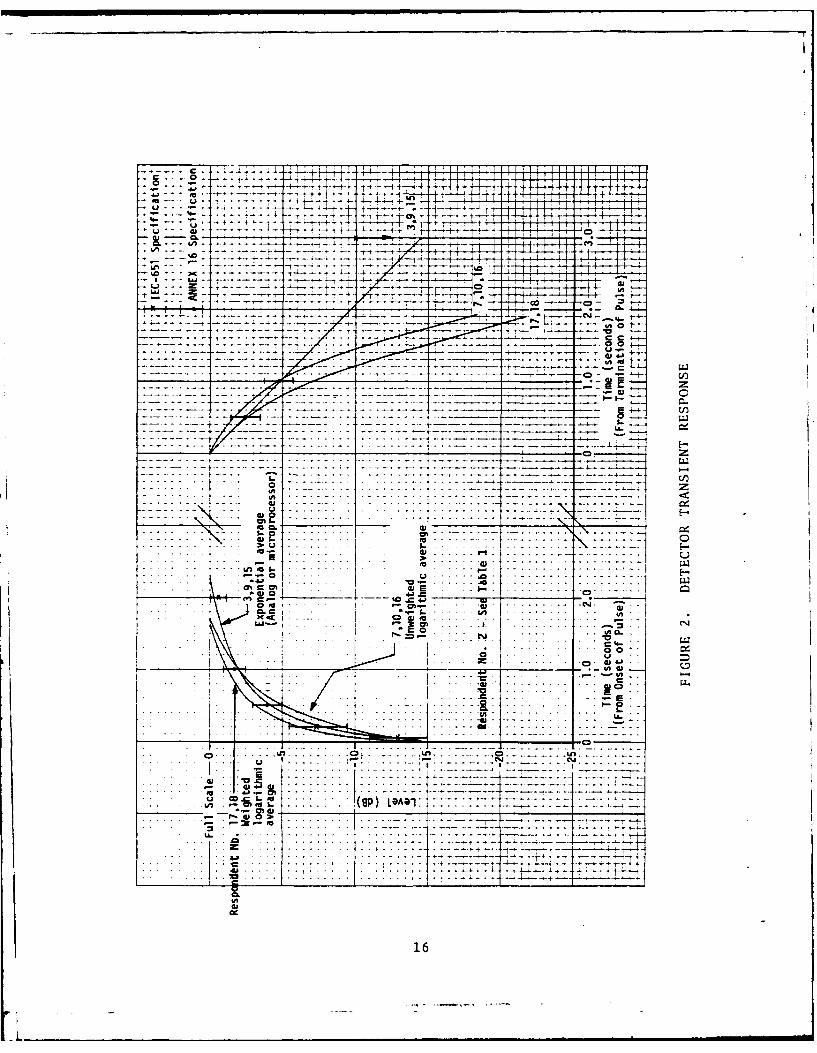
4.4 DETECTOR TRANSIENT RESPONSE
Figure 2 depicts the detector dynamic response characteristics
of the respondent's analysis system as obtained from the results
of test run 10. As shown, the results were grouped into three
distinct characteristic-curves which differ slightly both in
rise and fall characteristics. They however, meet the dynamic
detector specifications of Annex 16, Appendix 2, Section 3.4
which have been included in Figure 2 as vertical bars. The speci-
fications of IEC-651 (Reference 3) for type 0 sound level meters
are also included.
.Respondents 7, 10, 16, 17, and 18 used a sliding-window or
running-logarithmic average procedure, with data from three con-
secutive 0.5-second integration periods, to achieve the dynamic
response shown. The actual calculation procedure used by respon-
dents 17 and 18 differ slightly from that used by respondents
7, 10, 16, in that more "weight" is given to the later of the
three 0.S-second samples of data- The following relationship was
used to calculate the "weighted" logarithmic average:
iaveraged 10 1o 1 0 2 ( 0ISPLi-2) 0 (001 SPL0 1) 0.4S ( 1 0 0.1SPLi),
where i represents the sample number. The detector dynamic curve
of Figure 2 for respondents 17 and 18 can be characterized as
that of an exponential function with a nominal 750 millisecond
RC time constant.
Respondents 7, 10,and 16 applied equal weight to each of the
three 0.S-second samples of data; hence an unweighted logarithmic
average according to the following relationship:
SPLpaveraged - 10 log o1 0.33 (1 00.1SPLi,2) 0.33 (1 0 0.1SPLi) 0.33 (10 SPLi)
15
I. -_
-4 cc
1 7,
*~...1. lli __t
EU 41 a~.-. -4.
-1 - - - - - - -
16 06

The curve of Figure 2 for respondents 7, l0,and 16 can be
characterized as a quasi-exponential function with a nominal
750-millisecond RC time constant.
The dynamic detector characteristics for the remaining three
systems are obtained internally in the commercially packaged
systems (in one case by strictly analog circuitry; in a second
case, by a combination of an analog detector and continuous ex-
ponential averaging using microprocessor techniques; and, in the
third case, by digital and microprocessor techniques). The results
obtained for respondents 3, 9, and 15 are characterized by the ex-
ponential curve depicted in Figure 2 with a nominal 1000-milli-
second RC time constant.
An inspection of Figure 2 shows that the three curves meet
the Annex 16 requirements, however, only the exponential curve
with the 1000-msec RC time constant meets the 2.0-second sound
level meter specification of IEC 651. This long slow rise and
fall characteristic can result in slightly lower levels measured
for transient signals.
TSC has been experimenting with a 4-sample, weighted logarith-
mic average procedure to achieve an exponential detector character-
istic with an effective RC time constant of 1000 milliseconds;
thus approximating the dynamic detector curve of respondents 3, 9,
and 15. The following equation was used:
SL. 10 0.1 _1 0.. 0.39~. .2 (O0.SPL')]
xSavc 0.210 L 0.2 10
Reprocessing digital data stored on computer disk for testruns 11 through 14 using the TSC 4-sample, weighted logarithmic
averaging procedure (2.0 seconds averaging time) produced results
(PNL, PNLT) for test runs 11, 12, and 14 which were 0.1 to 0.2 dB
lower than those obtained using the same digital data and theabove 3-sample weighted procedure (1.5-second averaging time)
while results of 0.6 dB lower were calculated for test run 13
which contained signals with the most rapid transient changes.
17
- | i I-

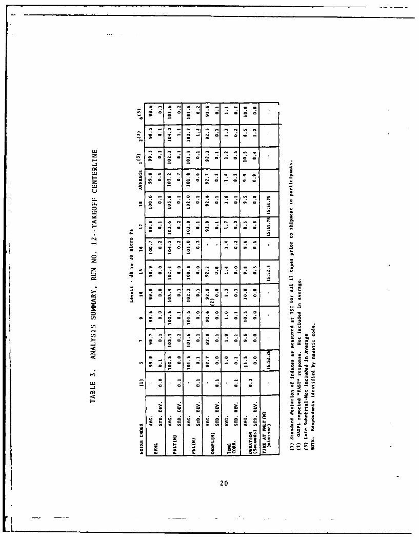
4.5 HELICOPTER NOISE DATA -- TEST RUNS 11, 12, 13, 14
Tables 2, 3, 4 and S summarize the results of respondents
processing the helicopter noise of test runs 11, 12, 13 and 14
respectively. Included (column 1) is a measure of the uniformity
of all seventeen tapes prior to shipment. The seventeen tapes
were analyzed at TSC using a GenRad®Y 1921 Real-Time Analyzer set
to integrate over 0.5-second periods. External computer smoothing
was used to achieve the dynamic detector requirements of Annex 16.
The tabulated respondents' data is the mean and standard de-
viations of four replications. (No adjustments have been made to
this data.) An inspection of Tables 2 through 5 show, in general,
a standard deviation of 0.2 dB or less was achieved by each re-
spondent, indicating a good within-organization repeatability.
Two exceptions are noted, respondent 15, test run 11, and re-
spondent 16, test runs 11, 12, 13,and 14. An examination of the
data submitted by respondent number 15 showed an apparent "noise
spike" in the third replication of test run number 11, affecting
in particular the tone correction calculation and the PNLTM
value. Excluding data from the third replication would have
reduced the standard deviation for test number 11 to 0.2 dB
or less, which is more in line with the rest of respondent 15's
submissions. Respondent 16 indicated he did not use the time
code signal provided to start the analyses. The non-standard
start times and a recorder amplitude instability problem, as in-
dicated by other data supplied by number 16, could account for
the high variability noted.
The average and standard deviation of the mean values sub-
mitted by all respondents are tabulated in column 10 of Tables
2 through 5. Note that those respondents who used the 250-Hz
calibration tone (respondents 3, 7, 10,and 15) reported consis-
tently lower results than those who used the 1000-Hz calibration
tone. As noted in Section 4.1, because of the manner in which
the raw data is stored on computer disc at TSC, it was possible
to reprocess the stored data referencing either calibration tone.
It was found that a -0.4 dB discrepancy was associated with the
18
L_...._. . .. . . . ..

v,~ -a a C C C
9 0; 0 0% 0 cc
a-
* a; - ; C; a ; - ; - ; W a
0; a a o % a -;
0 % NI Ol .fl
a
tj C
o a
C; C a a; a ; a - ; a a to a
00
- 0; a; a;C; 0 cc 0- ;
a 0.
in6-
-or 0% a a41-a 4 - - -zu "146u
o N a - a0%i% a 19I
L * ada a
4 -4!
p. ~ 4 -; 4 @0W S p 4 S
-at at a! a
-0 - -
OU
5'g
a in 4 a - 4 - na
I-I.
a a vs @4 @4 - a a a-2 a a a.4
- - - - - - - --6- zI.- 4.
a -4 4 a - - - u2a0

-1~~ 0 0 c;n00 a a a.
0 -a fta 0
- - S -I C 4c C; P -
S- C6411
a C! 4 C
US -0a I
a..
aa *
as a.Ul 6 i6 c 0 a
c cm - - -0 -
E - c a'
z3 ,. 4
a. a a.
41 - - - -21

-A @4 m~ - 0 o
0' C C; o 0
-~UI C C ' C! n C - C U
o1 C C 0
C t C! Ct 0
- 40
4- Cz C ;4 I.0
-. - -
-u . .
-- o
ri~ - - - - - -2

250-Hz calibration tone. This was traced back to the reference
tones and pink noise of the master tape-recording. Since the
deviation is a fixed function of the master recording, all tapes
would be affected equally; thus the submission of respondents
3, 7, 10,and 15 were adjusted by +0.4 dB to account for amplitude
differences in the calibration tones. The adjusted data wereplotted in Figures 3 through 6.
Note in Figures 3 through 6,the plotted tone corrections at the
time of PNLTM indicate a good correspondence in tone-correction-
factor calculation technique by all respondents. It is noted
that the maximum tone correction for the PNLTM spectrum was cal-
culated at the 160, 100, 100,and 100-Hz bands for test run numbers
11, 12, 13, and 14 respectively. According to the TSC procedure,
band-share corrections of 0.18 dB and 0.07 dB were calculated
for test runs 11 and 13 respectively. This data was not requested
of the participants and the TSC data is included for information.
An inspection of the data plots of Figures 3 through 6 shows
that results from respondents 15 and 16 control the spread of
data by consistently affecting the low and high value data points.It was noted earlier that a possible recorder amplitude instability
problem existed in the submissions by respondent number 16. It
is speculated that the higher-than-normal values reported by 16
may be traced to an erroneously reproduced amplitude calibration
reference level. This possibility has been discussed with res-
pondent 16 who has initiated an evaluation of the recorder used.The data submitted by respondent 16 is therefore not included in
the average and standard deviation values listed in Figures 3
through 6.
Nothing obvious was found from the data submitted by respon-dent number 15 to indicate why his results were consistently
lower than the average. It is, however, noted in Figure 2, that
respondent 15 along with respondents 3 and 9 processed data in
systems with a nominal one-second exponential time constant. A
close examination of the data in Figures 3 through 6 showed that
23. i

101.0IIIIIII T I III
I T1 .11 Average *99.1
99 ~ ~ ~ ~ ~ W D.v 0 0.5 11" 1111
I II II II .I II II II IStd. Dev. * 0.4
983.0-
101.- 7! II T I II iAverage 1091.8Std. Dev. - 0.3
1 2 .01 11 T I III I I Il I I II I I I
100.0Average 10.10 Std. 0ev. - 0.1
0~~~ ~ LIt smta-o inTue In average
2IUR 3. AUeraRe 9ATA8RUN ~ ~~ Sd NO. 1- 0.APRAH3ETELN
24
I T

100.0Average *99.9
Std. 0ev. - 0.4ME 444-
98.01:
100.0-
103.0- Average 102.
Std. Dev. - 0.3C ,-- 4
FETNDN CODif
NOTE DaaAw epne 6ntIcue naeae vae 11.
D1a0 bmte0.0ajstdb .. l
93. Lat su1rtao 1ncludedvenaave9a.e
FIGUREd 4.v SUMR DATA
2.05
-T I I I , T I i ; I

100 0-Average *99.6
Z Std. 0ev. - 0.4
98.0 -
Average *10L 1Std. Dev. *0.7
103.0.
Average *103.7I T Std. 0ev. - 0.6
102. 0.
93.0Average *93.4
91.0
2.0~.Averae - 1.5
Std. Dev. - 0.1
0 ~ I~IIiIII:IIIIIl~IIII1 23 6 7 9 10 15161718
RESPO#IOET CODENOTE: Data frm Respondent 16 not included in average values.(X)Respondent used 250..Hz :alibratlon tone.
Data submitted was adjusted by +0.4 dB.
13 Late submittal - not Included In average
FIGURE 5. SUMMARY DATA,RUN NO. 13-- FLYOVER CENTERLINE
26

j 106.0 111 T IITI I 111Average 106.3Std. 0ev. - 0.3
104.0
110.011 111 11TI
ji tS108.0 Average *108.0
Std. Dev. - 0.4
106.0
3 10. 0 Avrg 1 106.311 III
I ~ ~ ~ ~ ~ Sd Iev I 0.4 III1 111
1095.0 11111 1111. - IIIII'IWAverage 1095.Std. 0ev. *0.3
102.0 Avrg 1.
Std. Dev. *0.2
SM 0
1 23 6 7 9 10 1161118
Respondent CodeNOTE: Data from Respondent 16 not included in average values.(X)Respondent used 250-14z calibration tone.
Data submitted was adjusted by +0.4 dB.
0 Late riubmittal-not included in average
FIGURE 6. SUMMARY DATA,
RUN NO. 14-- FLYPAST CENTERLINE
27

the results from respondent 9 were also on the low side of the
average while results from respondent 3 were found to be at or
slightly on the low side of the average.
It was stated earlier that the long slow rise and fall
characteristic of the detectors with the one-second RC time con-
stant characteristic could produce levels slightly on the low
side when compared to the other techniques used by respondents
in this test. It is felt, however, that this is not the complete
explanation for the lower-than-average reading by respondent 15.
As shown in Table 1, four of eight respondents (No.'s 7, 16,
17, 18) used GenRad®Model 1921 Real-Time Analysis System and
external computer smoothing with a nominal RC time constant of750 milliseconds. Excluding data from number 16, as previously
mentioned, it can be shown that the variability (standard devia-
tion) between these three respondents is 0.2 dB or less for all
indexes reported for runs 11 through 14.
Comparing data from respondents 3, 9,and 15 (system with in-
ternal averaging and an effective 1000-msec RC time constant,
GenRad(- 1995, B&K 2131, B&K 2130) resulted in a variability (stan-
dard deviation) of all indexes for the four helicopter noise tests
of 0.5 dB or less.
Respondent number 10 used an FFT system and external computer
smoothing (unweighted logarithmic average). His results seem to
be consistently on the high side of the average data reported.
Number 10 reported several deviaticns in his analysis system which
was reported to be modified to conform as close as practicable (at
present) to the Annex 16 standard: for example, "deviation in
digital filter shapes may exist; also no "window" function was
applied to the FFT input data which can cause excessive leakage
between bands." These may account for the slightly higher-than-
average data.
The overall organization-to-organization variability (standard
deviation) is seen to be 0.5 dB or less for the noise indexes of
test runs 11, 12,and 14;and 0.7 dB or less is noted for test run
28
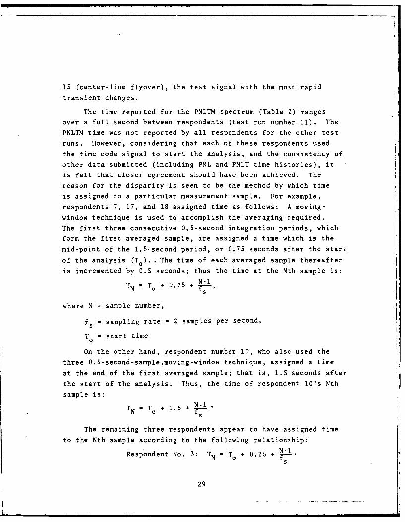
13 (center-line flyover), the test signal with the most rapid
transient changes.
The time reported for the PNLTM spectrum (Table 2) ranges
over a full second between respondents (test run number 11). The
PNLTM time was not reported by all respondents for the other test
runs. However, considering that each of these respondents used
the time code signal to start the analysis, and the consistency of
other data submitted (including PNL and PNLT time histories), it
is felt that closer agreement should have been achieved. The
reason for the disparity is seen to be the method by which time
is assigned to a particular measurement sample. For example,
respondents 7, 17, and 18 assigned time as follows: A moving-
window technique is used to accomplish the averaging required.
The first three consecutive 0.5-second integration periods, which
form the first averaged sample, are assigned a time which is the
mid-point of the 1.5-second period, or 0.75 seconds after the starL
of the analysis (T0 ).. The time of each averaged sample thereafter
is incremented by 0.5 seconds; thus the time at the Nth sample is:
TN T + 0.75 + N-1
where N = sample number,
fs a sampling rate - 2 samples per second,
T a start time
On the other hand, respondent number 10, who also used the
three 0.S-second-sample,moving-window technique, assigned a time
at the end of the first averaged sample; that is, 1.5 seconds after
the start of the analysis. Thus, the time of respondent 10's Nth
sample is:
TN - T + 1.5 + N-
The remaining three respondents appear to have assigned time
to the Nth sample according to the following relationship:N-l
Respondent No. 3: T = T + 0.25 + N---s
29
ii

N-1
Respondent No. 9: TN = 0 - 0.5 + Nf-P
Respondent No. 15: TN T o + NI
Appendix 2, paragraph 3.4.7 of Annex 16 states in part that
"the instant in time a readout is characterized shall be the mid-
point of the averaging period." The PNLTM times submitted by the
respondents indicate several possibilities; that is, (1) the above
specification was not complied with; (2) the system readout in-
troduced a positive or even negative timing error; or (3) the"averaging period" of the above specification needs clarification.
In analog exponential averaging using RC networks, the averag-
ing period (the time required for the network to charge to 87
percent or 0.6 dB of its final value) is defined as 2 times the RC
time constant of the network. It was shown in Section 4.4 that
the RC time constant was 750 milliseconds for the system used by
respondents 7, 10, 16, 17, and 18; and 1000 millisecond for the
systems used by respondents 3, 9,and 15. By the above definition
the averaging period would be 1.5 seconds and 2.0 seconds re-
spectively. The above averaging times and the individual system
output delay characteristics should be taken into account in time-
of-day assignments.
An additional subtle point in timing would be to be sure to
account for the time delay between the reproduced data and the
time code signal. For the NAGRA recorder used in this test, the
reproduced data lags 0.25 seconds behind a time code signal re-
produced from a CUE channel because of physical alignment of the
record and reproduce heads. None of the respondents accounted for
this delay.
4.6 DIGITAL DATA
Only two respondents used computer smoothing of the digital
data (respondents 7, 10). Both used a running-average technique
30
applying equal weighting (unweighted logarithmic average) to each
of the three 0.5-second data samples making up the average. In
order to provide a more consistent comparison between respondents,
the data submitted by respondents 7 and 10 were adjusted, based on
TSC's computations on un-averaged data and on data averaged using
the unweighted logarithmic procedure.
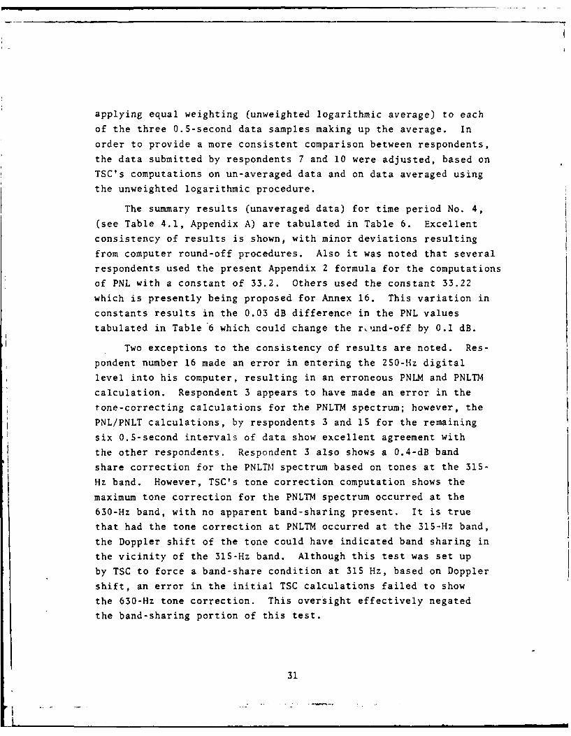
The summary results (unaveraged data) for time period No. 4,
(see Table 4.1, Appendix A) are tabulated in Table 6. Excellent
consistency of results is shown, with minor deviations resulting
from computer round-off procedures. Also it was noted that several
respondents used the present Appendix 2 formula for the computations
of PNL with a constant of 33.2. Others used the constant 33.22
which is presently being proposed for Annex 16. This variation in
constants results in the 0.03 dB difference in the PNL values
tabulated in Table 6 which could change the r, und-off by 0.1 dB.
Two exceptions to the consistency of results are noted. Res-
pondent number 16 made an error in entering the 250-Hz digital
level into his computer, resulting in an erroneous PNLM and PNLTM
calculation. Respondent 3 appears to have made an error in the
tone-correcting calculations for the PNLTM spectrum; however, the
PNL/PNLT calculations, by respondents 3 and 15 for the remaining
six 0.5-second intervals of data show excellent agreement with
the other respondents. Respondent 3 also shows a 0.4-dB band
share correction for the PNLTM spectrum based on tones at the 315-
Hz band. However, TSC's tone correction computation shows the
maximum tone correction for the PNLTM spectrum occurred at the
630-Hz band, with no apparent band-sharing present. It is true
that had the tone correction at PNLTM occurred at the 315-Hz band,
the Doppler shift of the tone could have indicated band sharing in
the vicinity of the 315-Hz band. Although this test was set up
by TSC to force a band-share condition at 315 Hz, based on Doppler
shift, an error in the initial TSC calculations failed to show
the 630-Hz tone correction. This oversight effectively negated
the band-sharing portion of this test.
31
. . .. .° .

v1 0
f 01 4) 4) K
00 W
+f +1 0 0- c U) .
0 11 0
0II 0 a0 N.
>1 0
w. 4D 0 o .+i 0 -o oo 01 00
C 0 o-~~4 01 .~ 0
0M 00 Z 4
41 44- -0 43 0 ,0
N~0 .j Ac,414 .
00 m. 0 0I 0
01 c
C; .4 4)
0% 0D C 0 -, 4 E..4
L 0 +, 0o WO~a04m0 u~ ' 00 a
a- - - -3 -- -Cc Z)
4-4 --- a' o 4 0 41*~~~" N0 r0*N uo . - 004
2 00 fg 0.1 U 0 M s-4 .. l. .0 01 1 e; CL inI-
9-a 43 'n u 0L z 14>3 4 00
-. 91 LL, a/ W. 0 : M u 61 v
3~ac .cc CU~
- 0C 433a1CL. o.1
32 _ 0 1U0
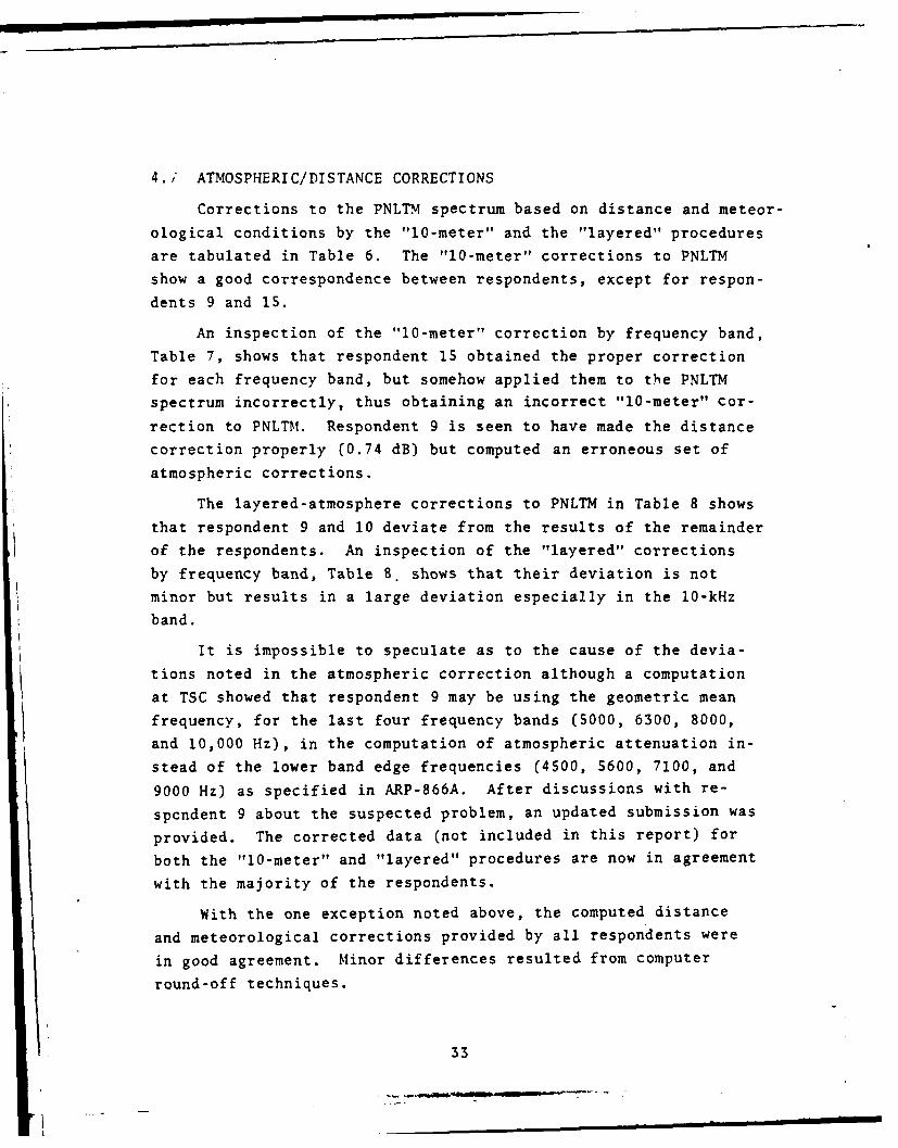
4./ ATMOSPHERIC/DISTANCE CORRECTIONS
Corrections to the PNLTM spectrum based on distance and meteor-
ological conditions by the "10-meter" and the "layered" procedures
are tabulated in Table 6. The "10-meter" corrections to PNLTM
show a good correspondence between respondents, except for respon-
dents 9 and 15.
An inspection of the "10-meter" correction by frequency band,
Table 7, shows that respondent 15 obtained the proper correction
for each frequency band, but somehow applied them to the PNLTM
spectrum incorrectly, thus obtaining an incorrect "10-meter" cor-
rection to PNLTM. Respondent 9 is seen to have made the distance
correction properly (0.74 dB) but computed an erroneous set of
atmospheric corrections.
The layered-atmosphere corrections to PNLTM in Table 8 shows
that respondent 9 and 10 deviate from the results of the remainder
of the respondents. An inspection of the "layered" corrections
by frequency band, Table 8. shows that their deviation is not
minor but results in a large deviation especially in the 10-kHz
band.
It is impossible to speculate as to the cause of the devia-
tions noted in the atmospheric correction although a computation
at TSC showed that respondent 9 may be using the geometric mean
frequency, for the last four frequency bands (5000, 6300, 8000,
and 10,000 Hz), in the computation of atmospheric attenuation in-
stead of the lower band edge frequencies (4500, 5600, 7100, and
9000 Hz) as specified in ARP-866A. After discussions with re-
spcndent 9 about the suspected problem, an updated submission was
provided. The corrected data (not included in this report) for
both the "10-meter" and "layered" procedures are now in agreement
with the majority of the respondents.
With the one exception noted above, the computed distance
and meteorological corrections provided by all respondents were
in good agreement. Minor differences resulted from computer
round-off techniques.
33

Cl.0
w W n n 1) 0 m LM %04m0
0!a!6
-I.-cocoa 0 a 00 00cca t 00 0c ceo c0 -100 ,G
zz
I., -nW D4 o1 Iv 0- r 0 00 0
ouor
(a 0
Ucc aaccc c c a ca c c a ..
., v uw ccu~, Lq.
a 0.
34,

000
00CC0 c0 o
0,O ,, 'D 405 C
0 C; 0 w ~ v ' cOSwN ' c c =;C ;
w. q. w- w- w. 1) M- In p. e4 r- .I- c -W r40. I's0 0 so cc4 .n noa
.4:0
zzo
p- -. 05
I!;___

5. CONCLUSIONS
1. Computations utilizing the digital data (3.5 seconds of a
simulated flyover) show excellent agreement among participants,
thus indicating good procedural application of the Annex 16
methodology for computation of noise indexes, such as PNL and
PNLT. A previous test on aircraft noise analysis (Reference 5)
concluded "a large part of the variations in results among
organizations was due to procedures" and therefore recommended
changes to be instituted.
2. With one exception, the computation of distance and mete-
orological corrections based on the "10-meter" and more complex
"layered" procedures were also in excellent agreement.
3. Band-sharing methodology (identification and adjustment for
important tones recorded in two adjacent 1/3-octave levels)
was not effectively tested with the digital data, however, a
common procedure for this adjustment should be specified by ICAO.
The FAR Part 36 Noise Standard, Reference 2, specifies a band-
sharing detection and adjustment procedure utilizing the
Doppler.shift phenomena. This procedure is used at TSC.
4. An inconsistent methodology was apparent in assigning time-of-
day to a sample of data. Time assigned is important since it
affects the apparent emission angle and noise propagation path
length, thus affecting the test-day-to-reference-day and
position corrections.
S. Although the transient response characteristics measured
(Figure 2) can be shown to meet the specifications of Annex 16
(Appendix 2 Section 3.4), the three typical curves shown are
uniquely different and the systems from which they were obtained
can respond differently under a variety of input noise situa-
tions. In spite of the small data set of this test, grouping
of the results can be seen. One group (variability 0.2 dB or
less) was formed by the data from respondents 7, 10, 16,and
18, who used external computer averaging with an effective RC
36

time constant of 750 milliseconds. A second group, although
not closely aligned (variability of 0.5 dB or less), was formed
by the data from respondents 3, 9, and 15, whose commercially
packaged systems were set to an effective RC time constant of
1000 milliseconds. A tighter specification by ICAO for the
detector characteristics is necessary.
6. The within-organization variability for the results of
test runs 11-14 (EPNL, PNL, PNLT) was shown to be 0.2 dB or
less. A reasonable organization-to-organization variability
of 0.5 dB or less was obtained for test runs 11, 12 and 14 and
0.7 dB or less for test run 13 which contained signals with
the most rapid transient changes.
Appreciation is again expressed to the participating organ-
izations. It is hoped that these results will serve to compensate
for the significant time expenditure volunteered for the conduct
of this Round-Robin Test.
37/38
-i-

APPENDIX A
TEST PROCEDUREAND
SAMPLE DATA-REPORTING SHEETS
(Note: certain data sheet page numbers have been omitted becausethey were duplicates of pages shown.)
A-1/A-2
' i - i • - - - - i i . . .
HELICOPTER NOI SE ANALYSI SROUND ROBIN TEST PROCEDURE
Edward J. Rlckley
January 1980
U.S. DEPARTMENT OF TRANSPORTATIONResearch and Special Programs Administration
Transportation Systems CenterEnvironmental Technology Branch
Cambridge, MA 02142
A-3

CONTENTS
1. Introduction
2. General
2.1 Test Tape
2.2 Digital Tabulation One-Third Octave Spectra
2.3 Instructions
3. Test Procedure Test Tape
3.1 Analysis System
3.2 Tape Recorder
3.3 System Calibration
3.4 Linearity Test
3.5 Detection Test
3.6 Pink Noise Test
3.7 Data Analysis
3.8 Calculations
3.9 Repeatibility of Analysis System
4. Digital Tabulations
4.1 Computer Averaging
4.2 As Measured PNL, dBA, OASPL
4.3 As Measured PNLT, PNLTM
4.4 Corrections to Reference Conditions
5. Data Reporting
'A-4

I. INTRODUCTION
At the October 1979 meeting of the International Civil Avia-
tion Organization, Committee on Aircraft Noise CICAO/CAN), Working
Group B, it was proposed that a round-robin test be conducted to
promote uniformity in the analysis of data for describing helicop-
ter noise for international helicopter certification standards.
The U.S. DOT/Transportation Systems Center (TSC) Kendall
Square, Cambridge, MA was requested by the Federal Aviation Admini-
stration Office of Energy and Environment to act as the focal point
for the definition of the test procedure and for the subsequent
collection and evaluation of results generated by the nations and
organizations participating. Accordingly TSC will generate a set
of identical helicopter noise test recordings, identify procedures
for their reduction, and distribute them to the participants for the
conduct of the test.
The test, sponsored by the Federal Aviation Administration,
Office of Energy and Environment, and proposed by the, International
Civil Aviation Organization, Committee on Aircraft Noise, is to
promote uniformity in the analysis of data for describing heli-
copter noise for international certification standards.
A-5

2. GENERAL
The complexity of helicopter flyby noise, which contains non-stationary random noise, fluctuating periodic signals and impulsivesignals, in combination with a variety of noise measurement anddata processing systems and procedures could result in a variationof flyby noise levels and descriptions measured for the same typeaircraft. The purpose of this round robin test is to evaluate thedata reduction systems and procedures to determine the magnitude ofthe variability between systems and organizations, identify poten-tial causes and assist in establishing recommended practices to
minimize the differences.
Each participant in the test will be provided with:
1) A test tape recording consisting of calibration andreference signals and noise data from three helicopter
flybys and one helicopter flypast.
2) Digital tabulations of one-third-octave band soundpressure levels in 0.5"second increments aroundPNLTM for a simulated flyover.
3) A set of instructions and standard data reporting
forms.
The participants will process the data using the instructions pro-vided and the procedures outlined in the ICAO International Stan-
dards and Recommended Practices on Aircraft Noise, Annex 16, Third
Edition, July 1978. At present Annex 16 does not apply to heli-copters until the recommendations of CAN 6 for helicopter standards
are incorporated as an amendment. The procedures of the Third
Edition supplemented by the appropriate CAN 6 recommendations willhowever be used in this test as specified in these test instruc-
tions.
2.1 TEST TAPE
The test tape recording contains noise data from three heli-copter flyovers and one flypast. Events were selected to include
A-6
tt.

pure tones, impulsive noise, broadband noise and psuedotones.
Included on the test recording are the following reference and
calibration signals for proper adjustment and calibration of the
data reduction system: a 1000 Hz pure tone signal provided at
four levels to determine the linearity of the data reduction sys-
tem; a series of tone'bursts to obtain a measure of detector
dynamic characteristics at 1000 Hz; and a standard IRIGB time code
signal recorded on a separate channel to provide exact synchroni-
zation of measurement periods. The contents of the test tape are
summarized below:
Run Data (Channel 1) Time Code Channel 2
1 Playback Reference Tone, 1000-Hz
2 Frequency Response Signal, Pink Noise
3 Amplitude Calibration, 250 Hz, 94dB
4 Amplitude Calibration, 500 Hz, 94dB
5 Amplitude Calibration, 1000 Hz, 94dB
6 Linearity Test Tone, 1000 Hz, 84dB
7 Linearity Test Tone, 1000 Hz, 74dB
8 Linearity Test Tone, 1000 Hz, 64dB
9 Linearity Test Tone, 1000 Hz, 54dB
10 Detector Test, 1000 Hz tone burst
11 Helicopter Flyover, Approach centerline
12 Helicopter Flyover, Takeoff centerline
13 Helicopter Flyover, Level Flightcenterline
14 Helicopter Flypast, Level Flightsideline
15 Playback Reference Tone, 1000 Hz
The master tape and the fifteen identical duplicate tapes were
recorded at a speed of 7 1/2 inches per second on a two track NAGRA
IVSJ recorder with Cue track. To insure that all copies were
identical, each tape was analyzed on the TSC analysis system
(GenRad 1921) before distribution to the participants.
A-7

2.2 DIGITAL TABULATIONS ONE-THIRD OCTAVE SPECTRA
One-third-octave digital sound pressure level data of a simu-lated flyover for seven consecutive 0.5 second periods around PNLTM
is supplied to each participant for processing through his com-
puter program that calculates PNL and PNLTM.
Processing of this digital data will allow investigation of
the possibility that variations in final results between partici-
pants in the analysis of the test tapes can be attributed tocalculation procedural differences, i.e., interpretation of defined
procedures or perhaps computer roundoff techniques.
2.3 INSTRUCTIONS
A set of instructions, including consideration of the latestproposed changes to Annex 16 are provided. Deviation from the pro-cedures must be minimized and where absolutely necessary a descrip-
tion of the deviation must be supplied. Standard data sheets areprovided for reporting all information requested for comparisonpurposes. Any other pertinent data that may influence the resultsshould be reported.
A-8

3. TEST PROCEDURE
3.1 ANALYSIS SYSTEM
The entire analysis system consisting of hardware and software
should comply with the requirements of the ICAO International
Standards and Recommended Practices on Aircraft Noise, Annex 16,
Appendix 2. One exception is oted, namely, the corrections for
spectral irregularities in Appendix 2, Paragraph 4.3 shall start at50 Hz instead of 80 Hz. Fill in the required information data
sheet pages 1 and 2. If "OTHER" was checked in box 4 or S on page1, explain fully on page 21. Explain any other special character-
istics of your analysis system that may not be adequately covered
by pages 1 and 2.
3.2 TAPE RECORDER
Using appropriate procedures set up channel 1 and 2 of thetape recorder for correct playback of the direct recorded signal
at a recorder speed of 7 1/2 inches per second. Run 1 playback
reference tone, should be used to adjust channel 1 and 2 of the
recorder electronics to full scale meter indication.
3.3 SYSTEM CALIBRATION
3.3.1 Playback the first reference tone (Run 1, channel 1).
Measure the frequency and level of reference tone. Signal should
be 1.0 ! 0.1 volt and 1000 + 10 Hz. Run 15 is a repeat of the
reference tone. Playback run 15 and measure the frequency andvoltage of reference tone. Tabulate voltage and frequency of runs
1 and 15 on the data sheet page 3.
3.3.2 Using the reference tone (Run 1, channel 1), adjust
electronics of analysis system for approximately full scale indica-
tion.
3.3.3 Run 3, 4, and 5 are acoustic calibration tones with a
sound pressure level of 94 dB re 20 micro Pascal at 250 Hz, 500 Hz, and
1000 Hz respectively with 0 dB gain. No gain or range corrections
A-9

are required with this tape. Playback the acoustic calibration
signal with the frequency that best suits you and adjust the
absolute calibration level of your system using the energy average
of twenty consecutive 1/2 second integration periods. Starting
at times indicated on data sheet, record the frequency of the
calibration signal used on the data sheet page 3.
3.4 LINEARITY TEST
Runs 5, 6, 7, 8, and 9 will be used to determine system
linearity. The energy average of twenty consecutive 1/2 second
integrations neriods should be determined. Playback runs 5, 6, 7,8, and 9 and start analysis at times indicated on data sheet.
Record the energy average at each level on the data sheet
provided page 3.
3.5 DETECTION TEST
To test the dynamic response characteristics at 1000 Hz ofeach participant's detection system a constant sinusoidal signal
followed by a series of tone bursts at 1000 Hz are provided as partof Run 10. The digital time history (consecutive 1/2 second dBvalues) of the RMS level of the 1000 Hz one-third octave band is
required from your analysis system. It is understood that somesystems require additional computer smoothing or averaging of the
analyzer output to conform to the dynamic response requirements ofAppendix 2, Paragraph 3.4.5. The digital history to be provided
must be processed in this manner.
3.5.1 Set the time constant or integration time of the analy-sis system to the desired value. Playback the recorded signal ofRun 10 and start the analysis at time 00:12:25 for a total of 86
seconds duration. Record the 172 consecutive digital outputs (onefor each 1/2 second) on the data sheet provided page 4. Alsorecord time constant or integration time. If computer smoothingwas used, explain the procedure employed on page 21.
A-10

3.6 PINK NOISE CALIBRATION
3.6.1 The pink noise signal (Run 2) should be processed
through the analysis system starting at time 00:02:04 for 40 con-
secutive 1/2 second integrations. A single value of the RMS level
for each of 24 one-third-octave bands (50 Hz-lOkHz) should be
obtained by energy averaging the 40 sets of data. Tabulate the
one-third-octave-band levels in dB on the supplied data sheet page
S.
3.6.2 Assuming a 0 dB correction for the one-third-octave bandwith a center-frequency to match the calibration signal used (sec-
tion 3.3.3), determine the corrections to be applied to each one-
third-octave-band to give a flat frequency response. Tabulate the
corrections on the data sheet page S. These corrections must be
applied to the data of the following operations.
3.7 DATA ANALYSIS
3.3.3 With the system calibrated as in section 3.2 and the
one-third-octave band corrections determined as in section 3.6,
the four recorded helicopter noise signals (Runs 11, 12, 13, 14)
will be processed through the calibrated analysis system and cal-
culation of noise descriptors performed. Since the noise signals
are recorded at the same gain as the acoustic calibration, no gain
corrections are required. Do not make any corrections for back-
ground noise.
3.7.1 Integration Time Set the time constant or integration
time to the value in section 3.S. Record time constant or inte-
gration time and computer smoothing procedure employed on data
sheet page 6.
3.7.2 Start Times and Duration Playback the signals of Runs
11, 12, 13, 14. The start time and duration of the analysis is
as follows:
A-il

Run Start Time Duration (seconds)
11- Approach centerline 00:14:50 2512- Takeoff centerline 00:15:42 2013- Flyover centerline 00:16:40 2014- Flypast centerline 00:17:31 35
Each event is to be analyzed over the total period given.
3.8 CALCULATIONS
The procedures of latest version of Section 4 Appendix 2 ofAnnex 16 must be used to determine EPNL and associated noise
indexes. All indexes will be calculated using the corrected 24one-third-octave bands of sound pressure levels.
For these computations it is to be assumed that actual andreference flight tracks are the same and that the reference mete-
orological conditions (25°C, 70% RH) apply to produce a set of"As Measured" indexes. The following information is required on
the data sheet pages 6-17 for Runs 11, 12, 13 and 14.
a) Time constant or integration time used.
b) Computer smoothing used, yes or no.
c) Start time and duration of data analysis
d) EPNL calculated in accordance with Annex 16, Appendix 2
procedures. (EPNdB)
e) Time of maximum PNLT (PNLTM) - (hr:min:sec).
f) Overall SPL for each 0.5 second interval (d).
g) Perceived Noise Level (PNL) for each 0.5 second interval
(PNdB).
h) Tone corrected Perceived Noise Level (PNLT)
for each 0.5 second interval (PNdB).
i) One-third octave band SPL's for the 0.5 second interval
at the time of PNLTM (dB).
A-12

3.9 REPEATABILITY OF ANALYSIS SYSTEM
The test procedure section 3 should be performed four times
to obtain a measure of the variance within each organization.
All data should be recorded in the data sheets provided
indentifying the repetition number.
A-13
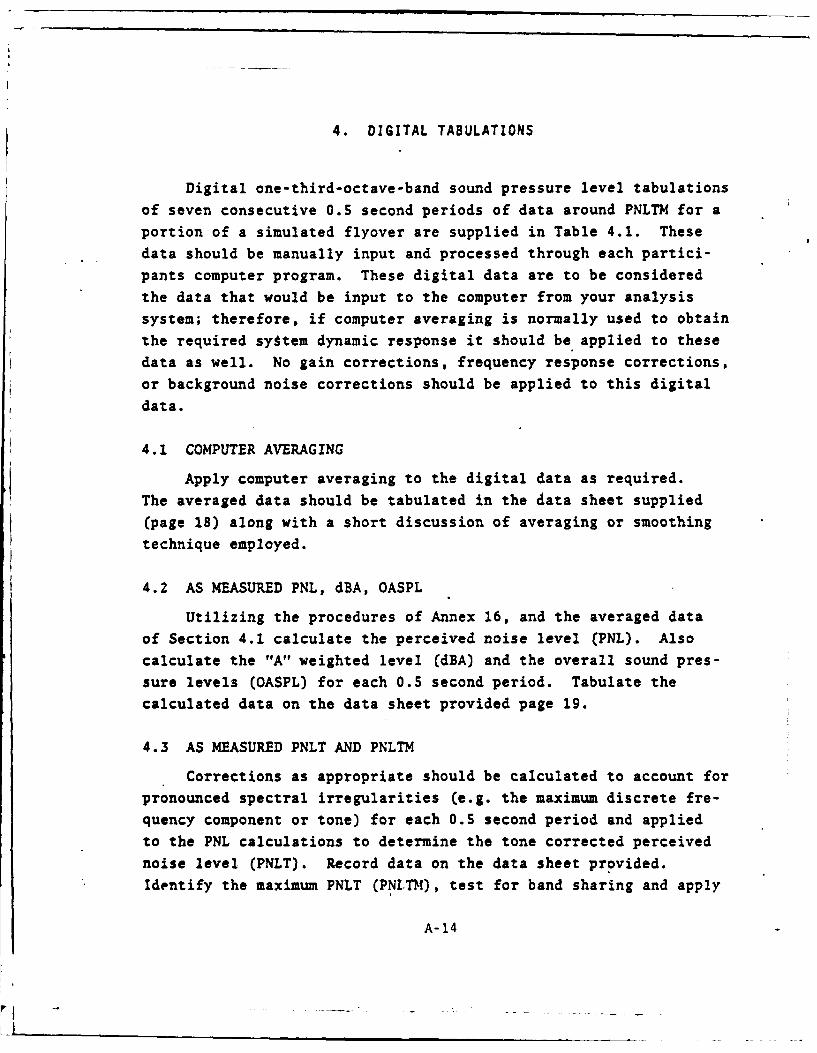
4. DIGITAL TABULATIONS
Digital one-third-octave-band sound pressure level tabulations
of seven consecutive 0.5 second periods of data around PNLTM for a
portion of a simulated flyover are supplied in Table 4.1. These
data should be manually input and processed through each partici-
pants computer program. These digital data are to be considered
the data that would be input to the computer from your analysis
system; therefore, if computer averaging is normally used to obtain
the required system dynamic response it should be applied to these
data as well. No gain corrections, frequency response corrections,
or background noise corrections should be applied to this digital
data.
4.1 COMPUTER AVERAGING
Apply computer averaging to the digital data as required.
The averaged data should be tabulated in the data sheet supplied
(page 18) along with a short discussion of averaging or smoothing
technique employed.
4.2 AS MEASURED PNL, dBA, OASPL
Utilizing the procedures of Annex 16, and the averaged dataof Section 4.1 calculate the perceived noise level (PNL). Also
calculate the "A" weighted level (dBA) and the overall sound pres-
sure levels (OASPL) for each 0.5 second period. Tabulate the
calculated data on the data sheet provided page 19.
4.3 AS MEASURED PNLT AND PNLTM
Corrections as appropriate should be calculated to account for
pronounced spectral irregularities (e.g. the maximum discrete fre-
quency component or tone) for each 0.5 second period and applied
to the PNL calculations to determine the tone corrected perceived
noise level (PNLT). Record data on the data sheet provided.
Identify the maximum PNLT (PNI.TM), test for band sharing and apply
A-14

the necessary band sharing correction. Record data on the data
sheet provided page 19.
4.4 CORRECTION TO REFERENCE CONDITIONS
Utilizing the flight track conditions as specified in Figure4.1 (where point Q is the aircraft position, in retarded time, at
the time of PNLTM) and the temperature humidity profile of Table4.2, the 1/3-octave spectra at PNLTM should be corrected for the
effects of atmospheric absorption and deviation from reference
flight track. The atmospheric attenuation of sound in air shall
be determined in accordance with the curves presented in SAE-ARP-
866A (3/15/75) the meteorological reference conditions are 25°C,70% RH).
4.4.1 Ten Meter Corrections Atmospheric absorption correc-
tions and distance correction should be calculated assuming the ten
meter meteorological data provided are constant throughout the
propagation path of the sound. Record data in the data sheet page
20.
4.4.2 Layered-Atmosphere Corrections The layered-atmosphereprocedure to correct the data for sound propagation in air using
SAE-ARP-866A is as follows:
a) Divide the sound propagation path into increments of 30meters in altitude.
b) Determine the average temperature and relative humidity
in each 30 meter altitude increment.
c) Calculate the atmospheric attenuation rate in each one-
third-octave-band in each altitude increment.
d) The mean atmospheric attenuation rate in each one-third-
octave-band over the complete propagation path must be
computed and used to calculate the corrections required.
Record atmospheric absorption and distance correction on data
sheet provided page 20.
A-l-j -_______A___ - 15-

5. DATA REPORTING
Fill out the data sheets reporting all information requested
for data comparison purposes. Any other pertinent data should be
reported if said data influences the data comparison between
analysis systems being employed by the various participants taking
part in the round robin test. All data should be mailed to:
Edward J. Rickley (Code DTS-331)U.S. Department of TransportationResearch and Special Programs AdministrationTransportation Systems CenterKendall SquareCambridge MA USA 02142Tel 617-494-2053
Participant organizations are not required to identify themselves.
All identities will be treated with the highest degree of con-
fidentiality,
A-16
• : $ ; . - •.. . .

Kror 106.3 Meters
.11l09
*115.8 meters
FIGURE 4.1 Flight path profile
A-17

i ~ ~ vI X
I
-. .' ,=.- -
S1 o
...
2 X 2 2 2
SIX a c il I l I,
*4.4° 4 - o-
$ t i
=1 8"
i i
fix'- *FK4S
-. * * *NA18
2 ; "1 2 2 1., .4 -I li * 5
211 1 " 2 2 . '
__ I I I II
U - N .45 ,
I '
-I S
1222-,1. 1
I| ;~~ ....
. . . . .. .. . . ... . .. . 2 ' , 3 . .

TABLE 4.2
ALTITUDE TEMPERATURE HUMIDITYMETERS !C %
10 12.0 90.0
30 11.2 85.6
60 10.0 79.0
90 8. 8 72.4
120 7.6 65.8
150 6.4 59.2
180 5.2 56.2
A-19/A-20
HELICOPTER NOISE ANALYSISROUND ROBIN TEST
DATA REPORTING SHEETS
Mall to: Noise Measurement andAssessment Laboratory (Code DTS-331)
U.S. DEPARTMENT OF TRANSPORTATIONResearch and Special Programs Administration
Transportation Systems CenterKendall Square
Cambridge, MA USA 02142
A2
A-21
~~1

-z~ ~ i- LLI
.2L LU3
z z CLUL I" C
mI- - Ix)I
I-U) u 0,
-h . .. a.
o at
________A CI U, .
Q- Go-191 11 I
cc U U u
- -U . Ln - m
- U = Z= - th =_ __7_ I- I- c r -
z 0 -C :1 A0 2
c 96 - - - L - z - - - - - -- - -0 A - ----j

Page 2
DATA SHEET
Please indicate whether or not your data analysis system complies withthe following requirements of Annex 16, Appendix 2 and other specialrequirements listed below.
YES NO
a) Dynamic characteristics of the RMS detector for rise andfall times of all one-third octave filters. c_1 t0
b) 0.5 second intervals must be 0.5 seconds + 0.01 second.
c) In cases where dead time occurs during readout andintegrator reset, the .loss shall not exceed 1% of the 0_ 0 _total data.
d) The levels from all 24 one-third-octave bands must beobtained within a 50 ms period. 510
e) The resolution of the digitizing system output shallbe equal to or better than 0.25 dB.
f) The detector must perform as a true mean square devicewith range and accuracies in agreement with Annex 16 [ LAppendix 2-3.4.3.
g) Tone correction procedures must be extended toinclude all bands from 50 Hz to 10 KHZ. 0
h) Tones that are recorded in two adjacent one-third octavebands must be compensated for. 0Explain the details of any checks in the "No" column onpage 21.
P-23
II I I" - - -

DATA SHEET PAGE 3
Pare, Enter the voltage and frequency of the3.3.1 reference tone.run1 & 1
REPETITION NO. 1 2 3 4
VOLTAGE RUN 1
VOLTAGE RUN 15
FREQUENCY RUN 1
FREQUENCY RUN iS
Pare. Check which calibration frequency was3.3.3 used. Energy average for 10 secondsrun after starting time.3-5
REPETITION NO. 1 2 3 4
250 Hz.Start - 00:03:20SOO Hz,Start - 00:04:21
5000 Hz.
Start - O0:OS:32
Para. Enter the measured RMS levels of the six3.4 1000 HZ. calibration signols. EnergyRun average for 10 seconds after starting time.5-9REPETITION NO. 1 2 3 4
RUN 5Start - 00:05:39
RUN 6Start - 00:06:56
RUN 7Start - 0O:08:l6
RUN 8Start 00:09:32
RUN* 9Start 00:10:50
A-24
K'

DATA SHEET PAGE 4a
Para. Record the digital time history of the 1000 Hz3.5.1 one-third octave band (band 30) for the 86 secondrun duration of that run.10 REPETITION NO. 1
Time constant or integration time used.
Smoothinz jsed- YES NO
(explain pg. 21)
A-25
V ______

DATA SHEET PAGE 5
Para. Tabulate the one-third octave sound pressure levels3.6 and corrections.run2
REPETITION NO.
2 3 4
FREQ. 0014q
50 HZ
63 HZ
80 HZ
100 HZ
125 HZ __i_ i
160 HZ
200 HZ
250 HZ
315 HZ400 HZ
500 HZ630 HZ
800 HZ
1 KHZ
1.2 KHZ
1.6 KHZ
2 KHZ
2.5 KHZ
3.1 KHZ4 KHZ
4 KHZ
6.3 KHZ
8 KHZ
10 KHZ
A-26

DATA SHEET PAGE 6
RUN 11
Para. Time constant or integration tie ased3.7&3.8Run Repetition No. 1 L . J11 i
Rep*tition No. 2
Repetitiin No. 3
Repetition No. 4 mSmoothing used ?
Repetition No. 1 YES NO
Rtpetition No. 2 YES NO
Repetitioh No. 3 YES F1 NO
Repetition No.4 YES NO
Start time and duration of the run.
Start Repetition No. 1 ::_. for sec.
Start Repetition No. 2 :. r _sec.
Start Repetition No. 3 ::. for sec..
Start Repetition No. 4 _e :.fr_ sec.
Calculated Effective Perceived Noise Level ( EPNL
Repetition No. 1
Repetitt-n No. 2
",~/Repetition No. 3 I IRepetition No. 4 I I
The time of maximum Tone Corrected Perceied Noise Level is-
Repetition No. 1
Repet .ti.on No. 2
Repetit4ion No. 3
Repetition No. 4A-27

DATA SHEET PAGE 7a
RUN 11
Para. Tabulate the Overall Sound Pressire Leel ( OASPL ),3.8 Perceived Noise Level ( PNL ), and Tone CorrectedRun Perceived Noise Level ( PNLT ).for tl'e entire ru n.11 Column headinqs 1 thro.ign 4 refer t3 the repetition no.
OrLPN PNfT 4
2 3 4 1 2 3 4 2 3
-.... - - - - -- a a - - ao- - - - -
-A8-
- I0 . a1
Continuled on Pg. 7b
A- 28
I n I I I

DATA SHEET Page 8
Para. Tabulate the one-third octave band levels at PNLTM time.3.8Run11
1 2 3 4FREQ SPL SPL SPL SPL
50 HZ
63 HZ
80 HZ
00 HZ
25 HZ
60 HZ
200 HZ
S0 HZ315 HZ
400 HZ
500 HZ
630 HZ
800 HZ
1 KHZ
1.2 KHZ1.6 KHZ
2 KHZ
2.5 KHZ
3.1 KHZ
4 KHZ
S KHZ6.3 KHZ8 _KHZ
10 KHZ
A-29

DATA SHEET PAGE 18
Para. If computer smoothing was used on the digital data4.1 from table 1, tabulate the resulting averaged data.
TIME TIME TIME TIME TIMEINTERVAL INTERVAL INTERVAL INTERVAL INTERVAL
FREQ 1 2 3 4 5
50 HZ
63 HZ
80 HZ
100 HZ
120 HZ
160 HZ
200 HZ
250 HZ315 HZ
400 HZ
S00 HZ
630 HZ
800 HZ1 ia'iz
1.2 KHZ1.6 KHZ2 IHZ2.5 KHZ __
3.1 KHZ4 KHZ
IS KHZ
6.3 KHZ8 K'HZ
10 KHZ
Provide a short discussion of averaging or smoothing employed.
A-30

wI
DATA SHEET PAGE 19
Para. Tabulate the calculated "A" Weighted SPL (dBA),4.2 Overall SPL (OASPL), Perceived Noise Level (PNL),
Tone Corrected Perceived Noise Level (PNLT), andidentify the Maximum PNLT (PNLTM).
TIME CHECKINTERVAL dBA OASPL PNL PNLT PNLTM
1
2
3
4
S
6
7
A-31
-~ --- .~~z~5 x- - C2T7~ -
Il l i iI • - . .. "

DATA SHEET PAGE 20
Para. Tabulate the corrections applied to the one-third4.4 octave band SPL's as a result of atmospheric absorption a
and distance correction using the 10 meter method andusing the layered atmosphere method.
10 LAYEREDFREQ METER ATMOS.
SO HZ __ _ _ _ _ _ _ _ _ _
63 HZ __ _ _ _ _ _ _ _ _ _
80 HZ ______ _____
100 HZ ______ _____
120 HZ ______ ___ __
160 HZ ______ _____
200 HZ _____
250 HZ _____ ____
315 HZ ______
400 HZ
SOO HZ
630 HZ ______ _____
800 NZ ______ ___ __
1 KHZ
1.2 KHZ __ _ _ _ __ ___
1.6 KHZ __ _ _ _ __ ___
2 KHZ _____
2.5 KHZ _____ ____
3.1 KHZ_____
4 KHZ __ _ _ _ _ _ _ _ _ _
S KHZ _____
6.3 ICHZ _____ _ _ _ _
8 KHZ ______
10 KHZ ___________
The corrected PNLTM is:
A-32

Page 21
DATA SHEET
A-33/A-34

REFERENCES
1. The International Standard and Recommended Practice,Aircraft Noise, Annex 16 to the Convention on International
Civil Aviation, Third Edition, July 1978. The International
Civil Aviation Organization (ICAO), Montreal, Canada.
2. The US/DOT/FAA Federal Aviation Regulations Part 36, Noise
Standards: Aircraft Type and Airworthiness Certification
(continuously amended). The Superintendent of Documents,
U.S. Government Printing Offices, Washington, DC 20402,
USA.
3. Publication 651, Instruments for the Measurement of Sound
Level (Sound Level Meters), 1st Edition 1979, The International
Electrotechnical Commission, Geneva, Switzerland.
4. Aerospace Recommended Practice (ARP) 866A, Standard Value
of Atmospheric Absorption as a Function of Temperature and
Humidity, Society of Automotive Engineers (SAE), Warrendale,
PA 15096, USA.
S. AIAA Paper No. 76-589, "Evaluation of Proposed Standards for
Aircraft Flyover Noise Analysis Systems," Stouder, D.J. and
McCann, J.C., American Institute of Aeronautics and Astro-nautics (AIAA), New York, NY 10019, USA.
450 copies
R-l/R-2

DAT
FILMEI
- II


