By: Marco Antonio Guimarães Dias Petrobras and PUC-Rio, Brazil

Visit the first real options website: www.puc-rio.br/marco.ind/

. Real Options in Petroleum:An Overview

Seminar Real Options in Real Life

MIT/Sloan School of Management - May 5th 2003

Seminar Outline Introduction and overview of real options in upstream

petroleum (exploration & production) Intuition, classical models, stochastic processes for oil prices

Brazilian applications of real options in petroleum Timing of Petroleum Sector Policy (extendible options) Petrobras research program called “PRAVAP-14” Valuation of

Development Projects under Uncertainties Focus on PUC-Rio projects.

Investment in information, real options and revelation Combination of technical and market uncertainties Assignment questions and the spreadsheet application

Managerial View of Real Options (RO) RO is a modern methodology for economic evaluation of

projects and investment decisions under uncertainty RO approach complements (not substitutes) the corporate tools (yet) Corporate diffusion of RO takes time and training

RO considers the uncertainties and the options (managerial flexibilities), giving two answers: The value of the investment opportunity (value of the option); and The optimal decision rule (threshold)

RO can be viewed as an optimization problem: Maximize the NPV (typical objective function) subject to: (a) Market uncertainties (eg.: oil price); (b) Technical uncertainties (eg., oil in place volume); and (c) Relevant Options (managerial flexibilities)

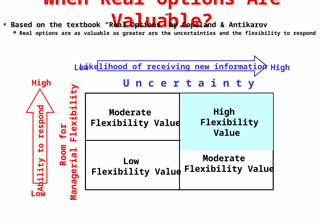
When Real Options Are Valuable? Based on the textbook “Real Options” by Copeland & Antikarov

Real options are as valuable as greater are the uncertainties and the flexibility to respondA

bili

ty t

o re

spon

d

Low

High

Likelihood of receiving new informationLow High

U n c e r t a i n t y

Roo

m f

or

Man

ager

ial F

lexi

bil

ity

Moderate Flexibility Value

Moderate Flexibility Value

Low Flexibility Value

High

Flexibility Value

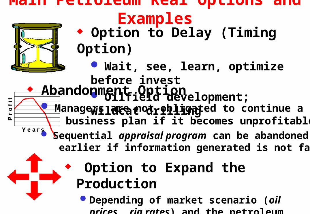
Main Petroleum Real Options and Examples

Option to Expand the Production Depending of market scenario (oil prices, rig rates)

and the petroleum reservoir behavior, new wells can be added to the production system

Option to Delay (Timing Option) Wait, see, learn, optimize before invest Oilfield development; wildcat drilling

Abandonment Option Managers are not obligated to continue a business plan if it becomes unprofitable Sequential appraisal program can be abandoned earlier if information generated is not favorable

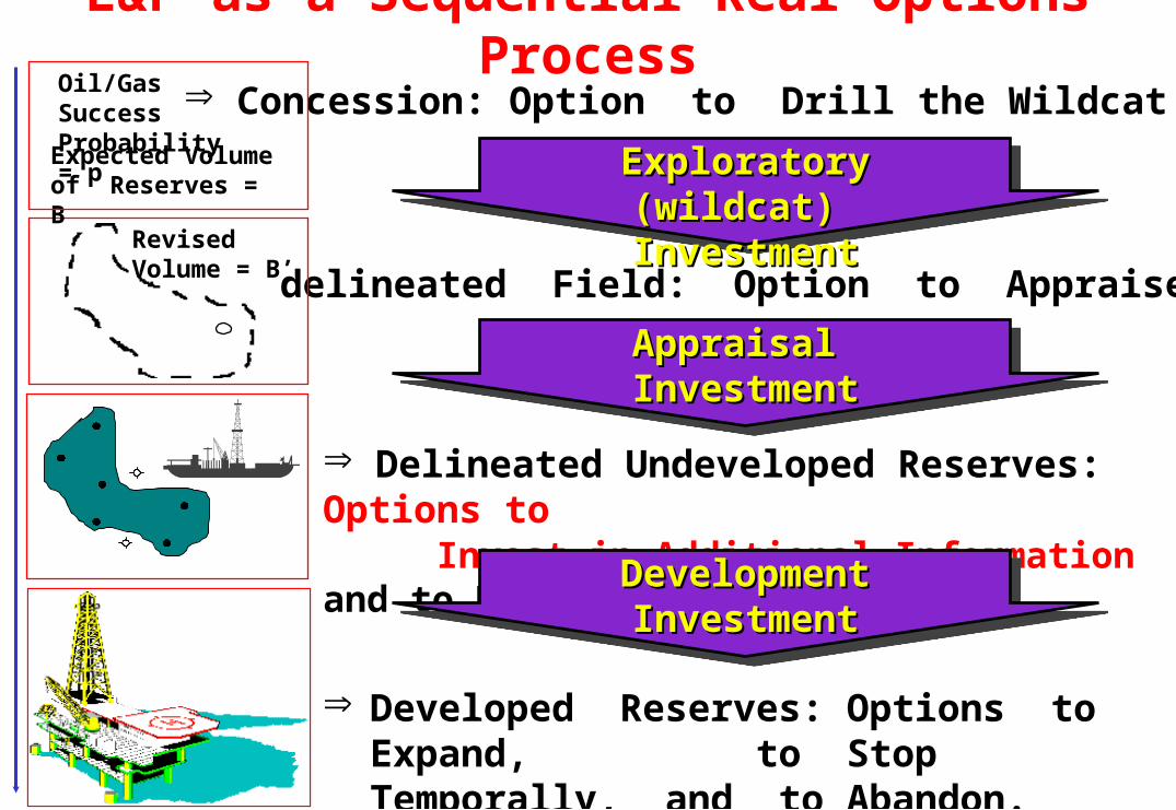
Undelineated Field: Option to Appraise

Appraisal Appraisal InvestmentInvestment

RevisedVolume = B’

Developed Reserves: Options to Expand, to Stop Temporally, and to Abandon.

E&P as a Sequential Real Options Process Concession: Option to Drill the Wildcat

Exploratory (wildcat) Exploratory (wildcat) InvestmentInvestment

Oil/Gas SuccessProbability = p

Expected Volumeof Reserves = B

Delineated Undeveloped Reserves: Options to Invest in Additional Information and to Develop

Development InvestmentDevelopment Investment

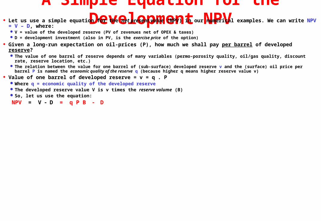
A Simple Equation for the Development NPV Let us use a simple equation for the net present value (NPV) in our numerical examples. We can write NPV = V – D, where:

V = value of the developed reserve (PV of revenues net of OPEX & taxes) D = development investment (also in PV, is the exercise price of the option)

Given a long-run expectation on oil-prices (P), how much we shall pay per barrel of developed reserve? The value of one barrel of reserve depends of many variables (permo-porosity quality, oil/gas quality, discount rate, reserve location, etc.) The relation between the value for one barrel of (sub-surface) developed reserve v and the (surface) oil price per barrel P is named the economic

quality of the reserve q (because higher q means higher reserve value v) Value of one barrel of developed reserve = v = q . P

Where q = economic quality of the developed reserve The developed reserve value V is v times the reserve volume (B) So, let us use the equation:

NPV = V D = q P B D

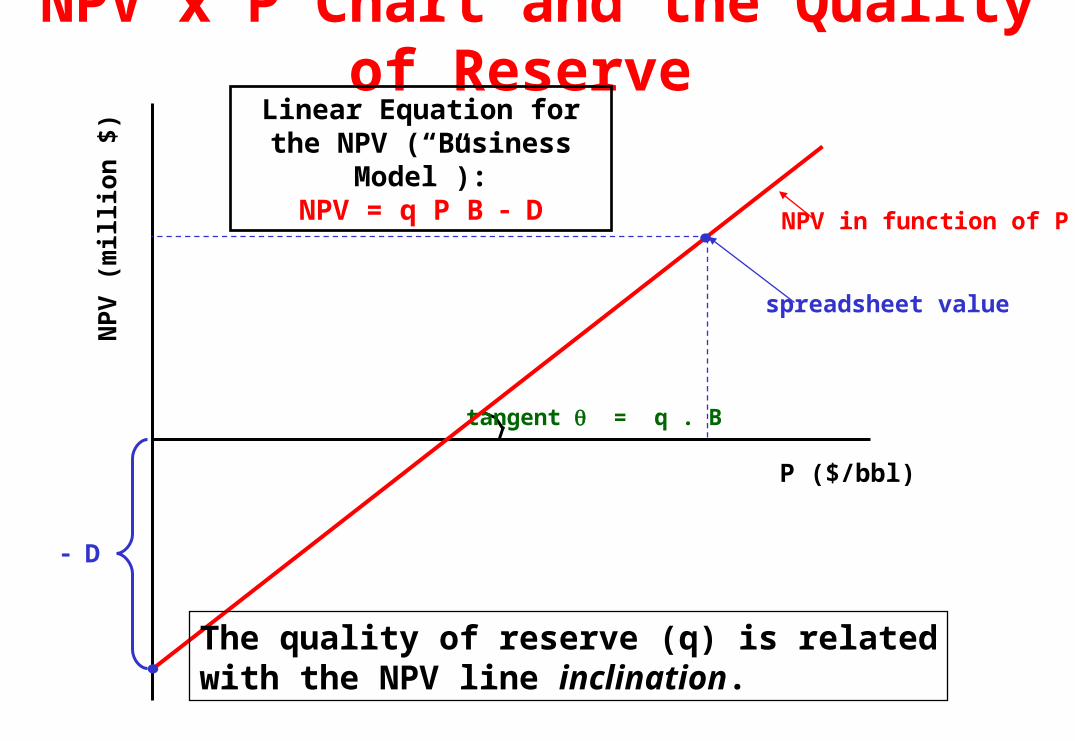
NPV x P Chart and the Quality of Reserve

tangent = q . B

D

P ($/bbl)

NP

V (

mil

lion

$)

Linear Equation for the NPV (“Business Model”):

NPV = q P B DNPV in function of P

The quality of reserve (q) is relatedwith the NPV line inclination.

spreadsheet value

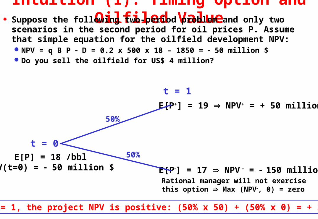
Intuition (1): Timing Option and Oilfiled Value Suppose the following two-period problem and only two scenarios in the

second period for oil prices P. Assume that simple equation for the oilfield development NPV: NPV = q B P D = 0.2 x 500 x 18 – 1850 = 50 million $ Do you sell the oilfield for US$ 4 million?

E[P] = 18 /bblNPV(t=0) = 50 million $

E[P+] = 19 NPV+ = + 50 million $

E[P] = 17 NPV = 150 million $

Rational manager will not exercise this option Max (NPV, 0) = zero

Hence, at t = 1, the project NPV is positive: (50% x 50) + (50% x 0) = + 25 million $

50%

50%

t = 1

t = 0

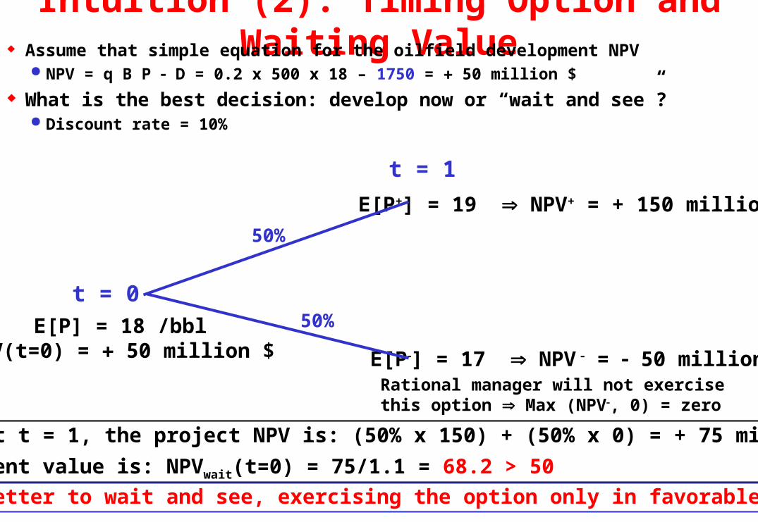
Intuition (2): Timing Option and Waiting Value Assume that simple equation for the oilfield development NPV

NPV = q B P D = 0.2 x 500 x 18 – 1750 = 50 million $

What is the best decision: develop now or “wait and see”? Discount rate = 10%

E[P] = 18 /bblNPV(t=0) = 50 million $

E[P+] = 19 NPV+ = + 150 million $

E[P] = 17 NPV = 50 million $

Rational manager will not exercise this option Max (NPV, 0) = zero

Hence, at t = 1, the project NPV is: (50% x 150) + (50% x 0) = + 75 million $

The present value is: NPVwait(t=0) = 75/1.1 = 68.2 > 50

50%

50%

t = 1

t = 0

Hence is better to wait and see, exercising the option only in favorable scenario

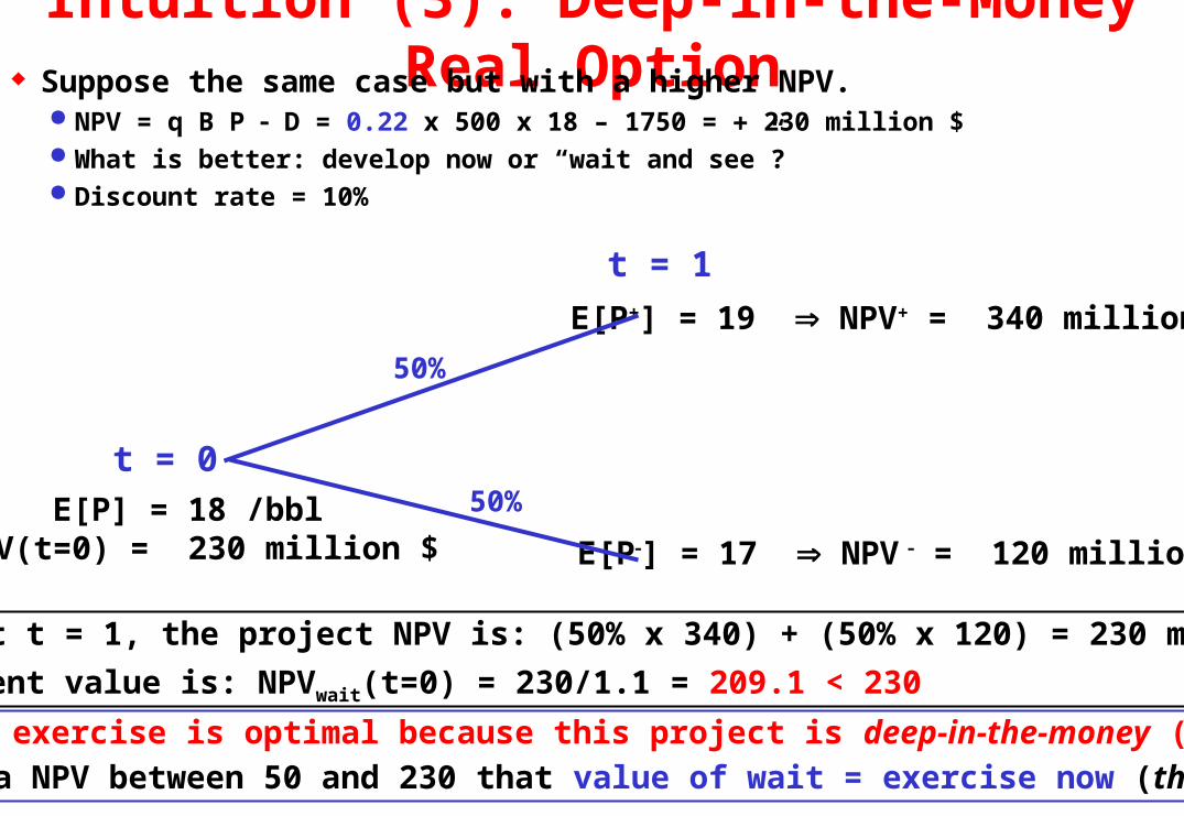
Intuition (3): Deep-in-the-Money Real Option Suppose the same case but with a higher NPV.

NPV = q B P D = 0.22 x 500 x 18 – 1750 = 230 million $ What is better: develop now or “wait and see”? Discount rate = 10%

E[P] = 18 /bbl NPV(t=0) = 230 million $

E[P+] = 19 NPV+ = 340 million $

E[P] = 17 NPV = 120 million $

Hence, at t = 1, the project NPV is: (50% x 340) + (50% x 120) = 230 million $

The present value is: NPVwait(t=0) = 230/1.1 = 209.1 < 230

50%

50%

t = 1

t = 0

Immediate exercise is optimal because this project is deep-in-the-money (high NPV)

There is a NPV between 50 and 230 that value of wait = exercise now (threshold)

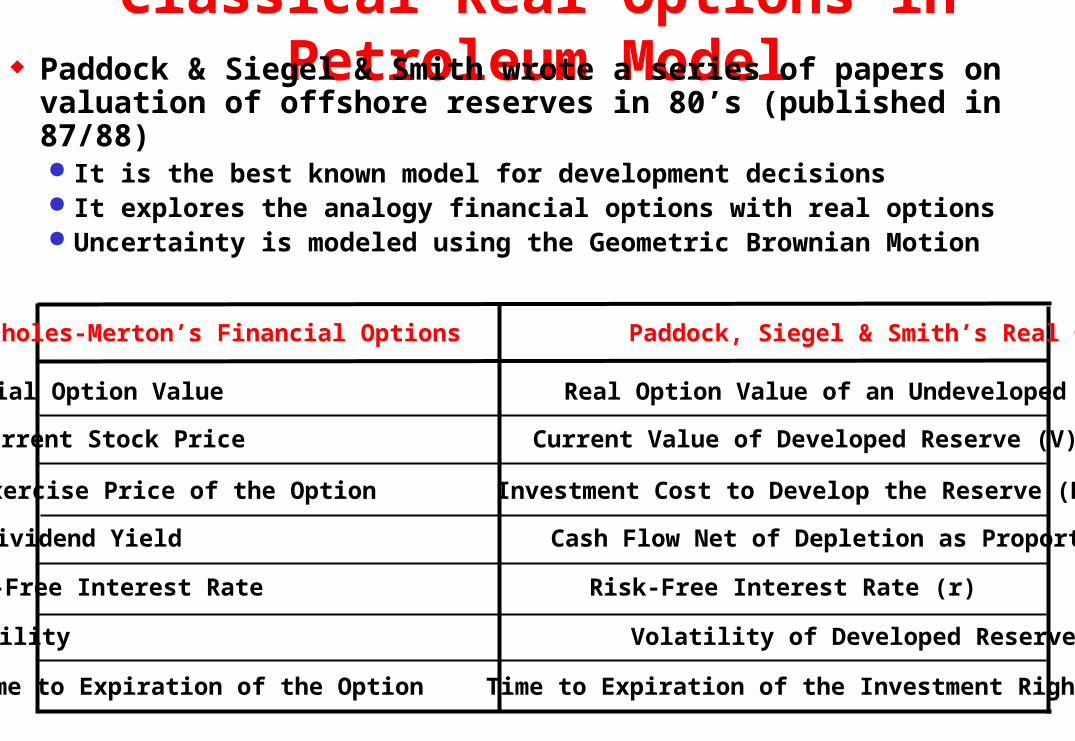
Classical Real Options in Petroleum Model Paddock & Siegel & Smith wrote a series of papers on

valuation of offshore reserves in 80’s (published in 87/88) It is the best known model for development decisions It explores the analogy financial options with real options Uncertainty is modeled using the Geometric Brownian Motion

Black-Scholes-Merton’s Financial Options Paddock, Siegel & Smith’s Real Options

Financial Option Value Real Option Value of an Undeveloped Reserve (F)

Current Stock Price Current Value of Developed Reserve (V)

Exercise Price of the Option Investment Cost to Develop the Reserve (D)

Stock Dividend Yield Cash Flow Net of Depletion as Proportion of V ()

Risk-Free Interest Rate Risk-Free Interest Rate (r)

Stock Volatility Volatility of Developed Reserve Value ()

Time to Expiration of the Option Time to Expiration of the Investment Rights ()

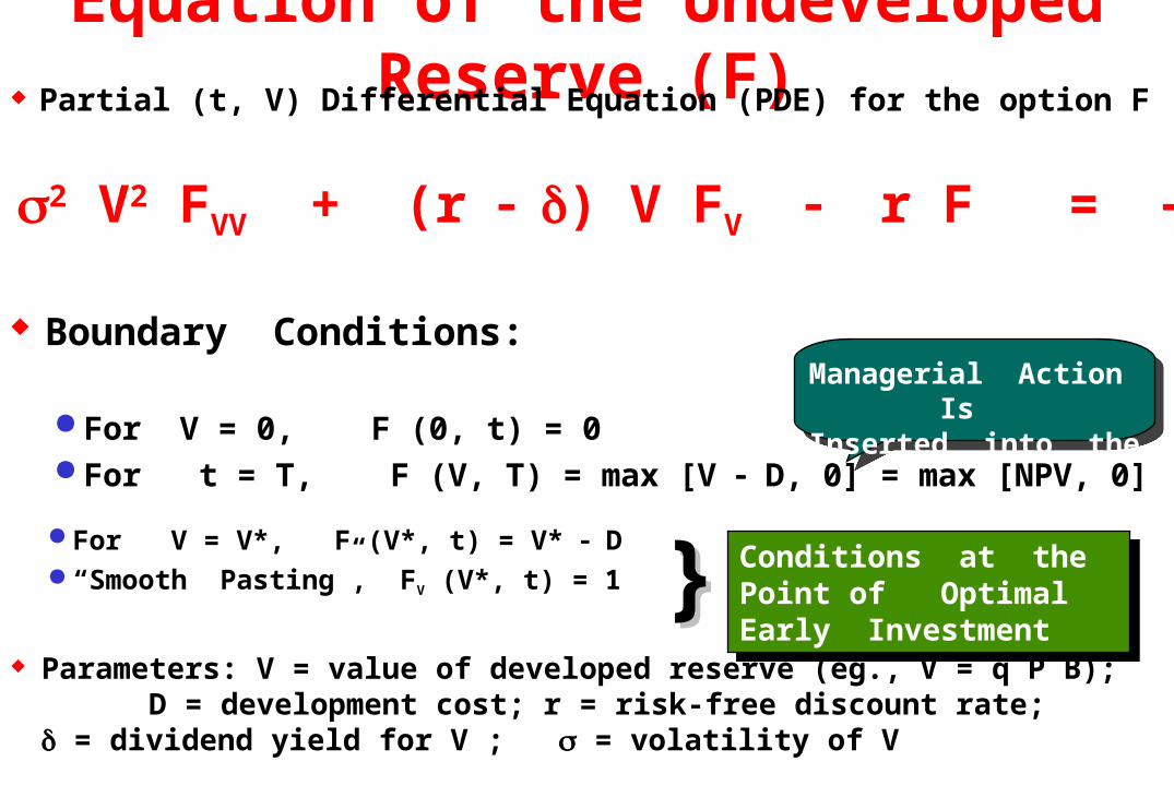
Equation of the Undeveloped Reserve (F) Partial (t, V) Differential Equation (PDE) for the option F

Managerial Action Is Inserted into the Model

Boundary Conditions:

For V = 0, F (0, t) = 0 For t = T, F (V, T) = max [V D, 0] = max [NPV, 0]

}} Conditions at the Point of Optimal Early Investment

Conditions at the Point of Optimal Early Investment

For V = V*, F (V*, t) = V* D “Smooth Pasting”, FV (V*, t) = 1

Parameters: V = value of developed reserve (eg., V = q P B); D = development cost; r = risk-free discount rate; = dividend yield for V ; = volatility of V

0.5 2 V2 FVV + (r ) V FV r F = Ft

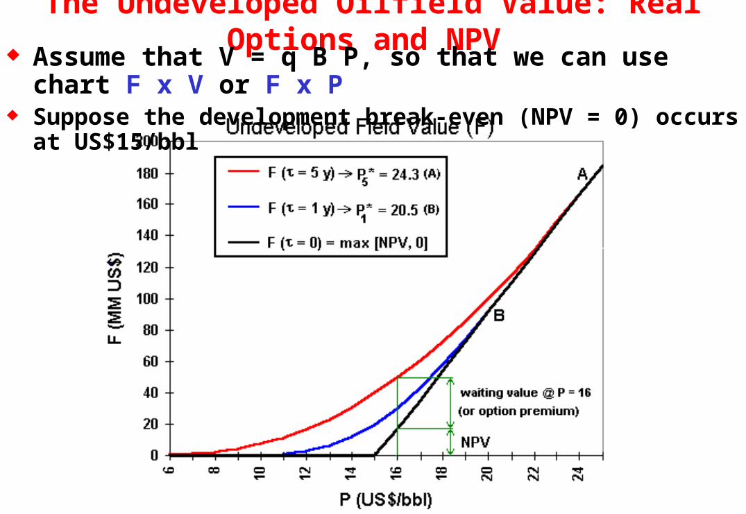
The Undeveloped Oilfield Value: Real Options and NPV Assume that V = q B P, so that we can use chart F x V or F x P

Suppose the development break-even (NPV = 0) occurs at US$15/bbl

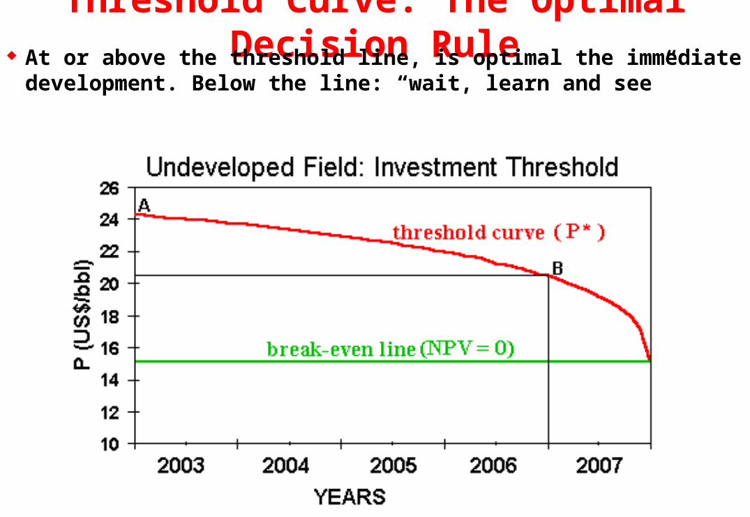
Threshold Curve: The Optimal Decision Rule At or above the threshold line, is optimal the immediate

development. Below the line: “wait, learn and see”

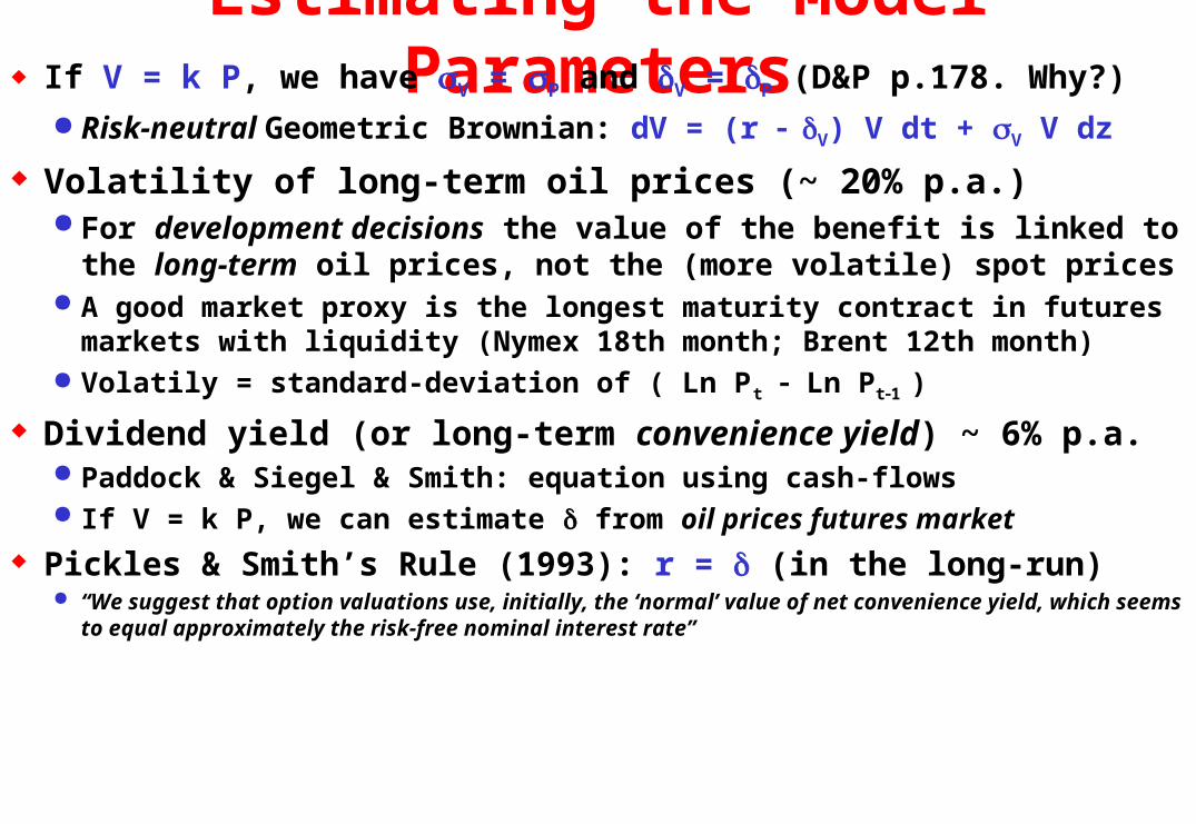
Estimating the Model Parameters If V = k P, we have V = P and V = P (D&P p.178. Why?)

Risk-neutral Geometric Brownian: dV = (r V) V dt + V V dz

Volatility of long-term oil prices (~ 20% p.a.) For development decisions the value of the benefit is linked to the long-term oil

prices, not the (more volatile) spot prices A good market proxy is the longest maturity contract in futures markets with

liquidity (Nymex 18th month; Brent 12th month) Volatily = standard-deviation of ( Ln Pt Ln Pt1 )

Dividend yield (or long-term convenience yield) ~ 6% p.a. Paddock & Siegel & Smith: equation using cash-flows If V = k P, we can estimate from oil prices futures market

Pickles & Smith’s Rule (1993): r = (in the long-run) “We suggest that option valuations use, initially, the ‘normal’ value of net convenience yield, which seems to

equal approximately the risk-free nominal interest rate”

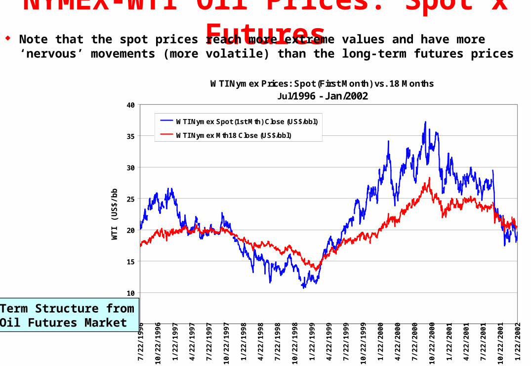
NYMEX-WTI Oil Prices: Spot x Futures Note that the spot prices reach more extreme values and have more

‘nervous’ movements (more volatile) than the long-term futures pricesWTI Nymex Prices: Spot (First Month) vs. 18 Months

Jul/1996 - Jan/2002

5

10

15

20

25

30

35

40

7/22

/199

6

10/2

2/19

96

1/22

/199

7

4/22

/199

7

7/22

/199

7

10/2

2/19

97

1/22

/199

8

4/22

/199

8

7/22

/199

8

10/2

2/19

98

1/22

/199

9

4/22

/199

9

7/22

/199

9

10/2

2/19

99

1/22

/200

0

4/22

/200

0

7/22

/200

0

10/2

2/20

00

1/22

/200

1

4/22

/200

1

7/22

/200

1

10/2

2/20

01

1/22

/200

2

WT

I (U

S$/

bb

l) WTI Nymex Spot (1st Mth) Close (US$/bbl)

WTI Nymex Mth18 Close (US$/bbl)

Term Structure fromOil Futures Market

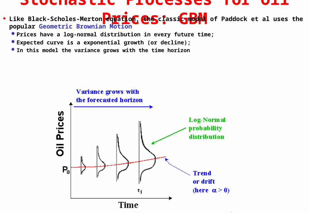
Stochastic Processes for Oil Prices: GBM Like Black-Scholes-Merton equation, the classic model of Paddock et al uses the popular Geometric

Brownian Motion Prices have a log-normal distribution in every future time; Expected curve is a exponential growth (or decline); In this model the variance grows with the time horizon

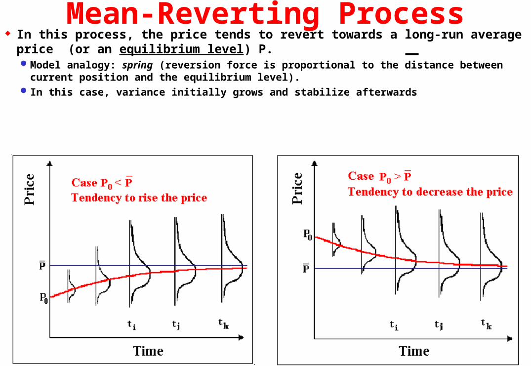
In this process, the price tends to revert towards a long-run average price (or an equilibrium level) P. Model analogy: spring (reversion force is proportional to the distance between current position and the

equilibrium level). In this case, variance initially grows and stabilize afterwards

Mean-Reverting Process

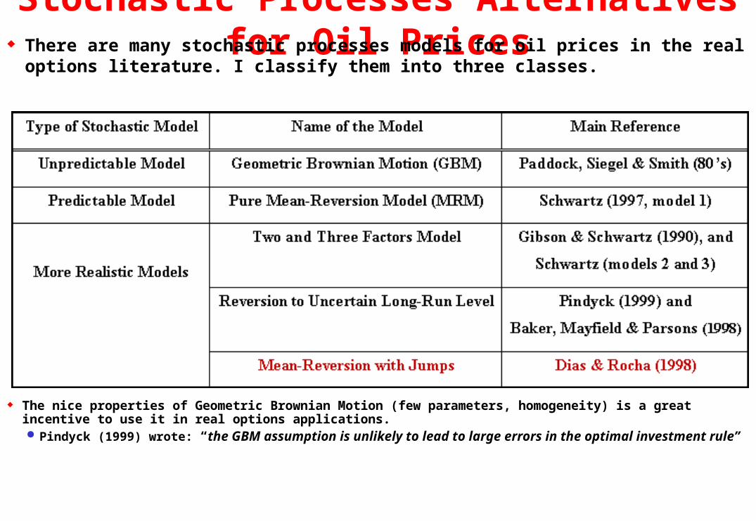
Stochastic Processes Alternatives for Oil Prices There are many stochastic processes models for oil prices in the real

options literature. I classify them into three classes.

The nice properties of Geometric Brownian Motion (few parameters, homogeneity) is a great incentive to use it in real options applications. Pindyck (1999) wrote: “the GBM assumption is unlikely to lead to large errors in the optimal investment rule”

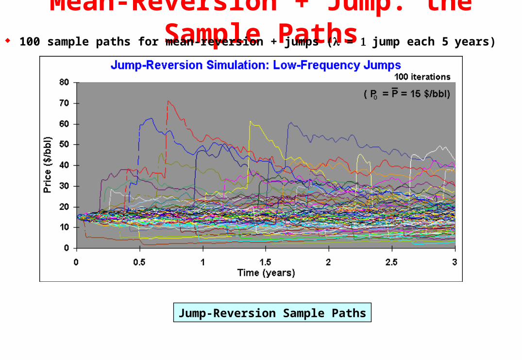
Mean-Reversion + Jump: the Sample Paths 100 sample paths for mean-reversion + jumps ( = jump each 5years)

Jump-Reversion Sample Paths

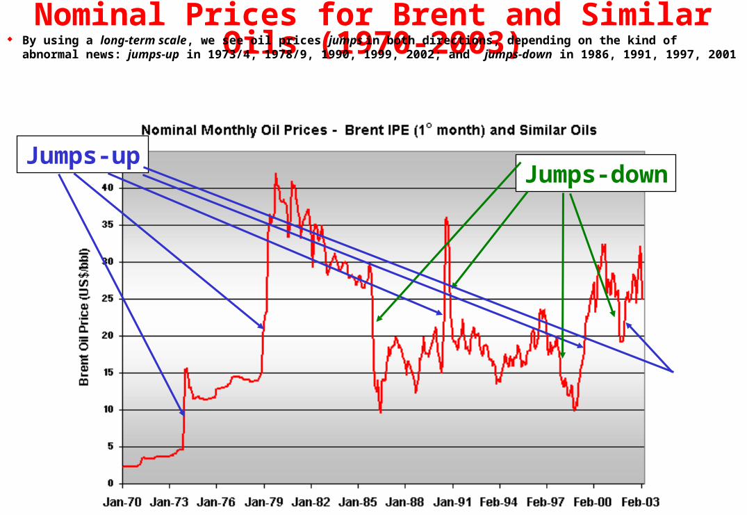
Nominal Prices for Brent and Similar Oils (1970-2003) By using a long-term scale, we see oil prices jumps in both directions, depending on the kind of abnormal

news: jumps-up in 1973/4, 1978/9, 1990, 1999, 2002; and jumps-down in 1986, 1991, 1997, 2001

Jumps-upJumps-down

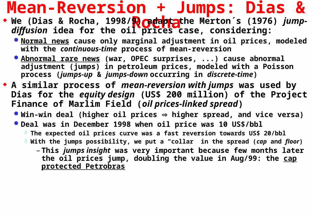
Mean-Reversion + Jumps: Dias & Rocha We (Dias & Rocha, 1998/9) adapt the Merton´s (1976) jump-diffusion

idea for the oil prices case, considering: Normal news cause only marginal adjustment in oil prices, modeled with the

continuous-time process of mean-reversion Abnormal rare news (war, OPEC surprises, ...) cause abnormal adjustment

(jumps) in petroleum prices, modeled with a Poisson process (jumps-up & jumps-down occurring in discrete-time)

A similar process of mean-reversion with jumps was used by Dias for the equity design (US$ 200 million) of the Project Finance of Marlim Field (oil prices-linked spread) Win-win deal (higher oil prices higher spread, and vice versa) Deal was in December 1998 when oil price was 10 US$/bbl

The expected oil prices curve was a fast reversion towards US$ 20/bbl With the jumps possibility, we put a “collar” in the spread (cap and floor)

– This jumps insight was very important because few months later the oil prices jump, doubling the value in Aug/99: the cap protected Petrobras

Brazilian Timing Policy for the Oil Sector The Brazilian petroleum sector opening started in 1997, breaking the Petrobras’

monopoly. For E&P case: Fiscal regime of concessions, with first-price sealed bid (like USA) Adopted the concept of extendible options (two or three periods).

The time extension is conditional to additional exploratory commitment (1-3 wells), established before the bid (it is not like Antamina)

The extendible feature occurred also in USA (5 + 3 years, for some areas of GoM) and in Europe (see paper of Kemna, 1993)

Options with extendible maturities was studied by Longstaff (1990) for financial applications The timing for exploratory phase (time to expiration for the development rights) was object of a

public debate The National Petroleum Agency posted the first project for debate in its website in February/1998, with 3 + 2 years,

time we considered too short Dias & Rocha wrote a paper on this subject, presented first in May 1998.

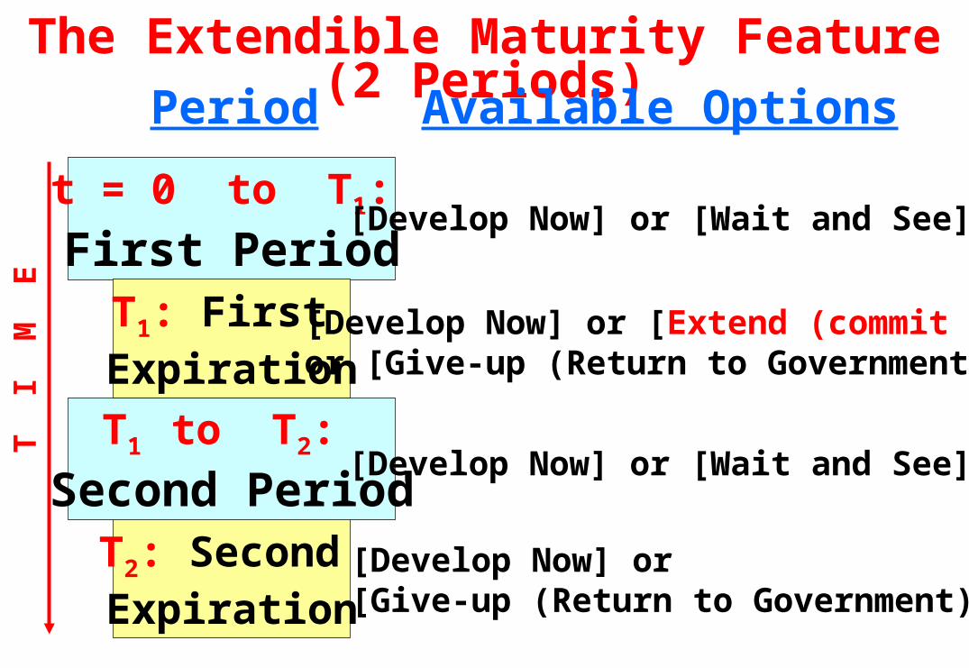
The Extendible Maturity Feature (2 Periods)

T2: Second Expiration

t = 0 to T1:

First PeriodT1: First

Expiration

T1 to T2:

Second Period

[Develop Now] or [Wait and See]

[Develop Now] or [Extend (commit K)] or [Give-up (Return to Government)]

T I

M E

Period Available Options

[Develop Now] or [Wait and See]

[Develop Now] or [Give-up (Return to Government)]

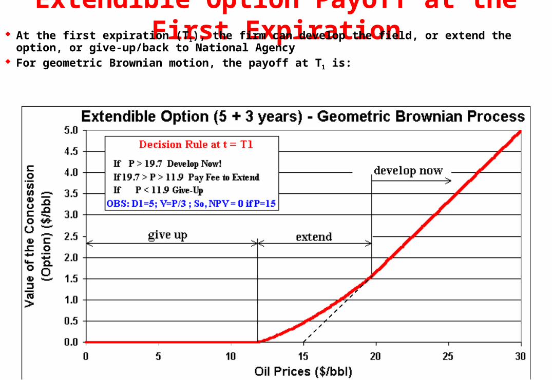
Extendible Option Payoff at the First Expiration At the first expiration (T1), the firm can develop the field, or extend the option, or give-up/back to National

Agency For geometric Brownian motion, the payoff at T1 is:

Debate of Timing of Petroleum Policy The oil companies considered very short the time of 3 + 2 years that

appeared in the first draft by National Agency It was below the international practice mainly for deepwaters areas (e.g.,

USA/GoM: some areas 5 + 3 years; others 10 years) During 1998 and part of 1999, the Director of the National Petroleum Agency

(ANP) insisted in this short timing policy The numerical simulations of our paper (Dias & Rocha, 1998) concludes that

the optimal timing policy should be 8 to 10 years In January 1999 we sent our paper to the notable economist, politic and ex-

Minister Delfim Netto, highlighting this conclusion In April/99 (3 months before the first bid), Delfim Netto wrote an article at

Folha de São Paulo (a top Brazilian newspaper) defending a longer timing policy for petroleum sector

Delfim used our paper conclusions to support his view! Few days after, the ANP Director finally changed his position!

Since the 1st bid most areas have 9 years. At least it’s a coincidence!

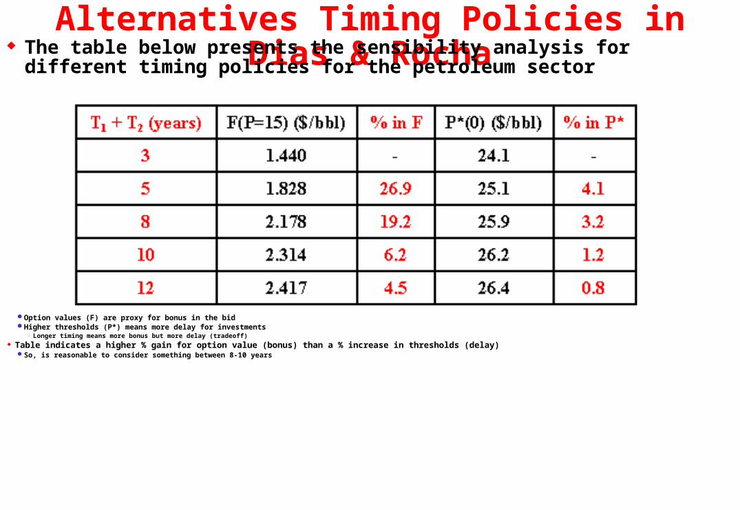
Alternatives Timing Policies in Dias & Rocha The table below presents the sensibility analysis for different timing policies for the

petroleum sector

Option values (F) are proxy for bonus in the bid Higher thresholds (P*) means more delay for investments

Longer timing means more bonus but more delay (tradeoff) Table indicates a higher % gain for option value (bonus) than a % increase in thresholds (delay)

So, is reasonable to consider something between 8-10 years

PRAVAP-14: Some Real Options Projects PRAVAP-14 is a systemic research program named Valuation of

Development Projects under Uncertainties I coordinate this systemic project by Petrobras/E&P-Corporative

I’ll present some developed real options projects: Exploratory revelation with focus in bids (pre-PRAVAP-14) Dynamic value of information for development projects Selection of mutually exclusive alternatives of development investment under

oil prices uncertainty (with PUC-Rio) Analysis of alternatives of development with option to expand, considering

both oil price and technical uncertainties (with PUC) We analyze different stochastic processes and solution methods

Geometric Brownian, reversion + jumps, different mean-reversion models Finite differences, Monte Carlo for American options, genetic algorithms Genetic algorithms are used for optimization (thresholds curves evolution)

I call this method of evolutionary real options (I have two papers on this)

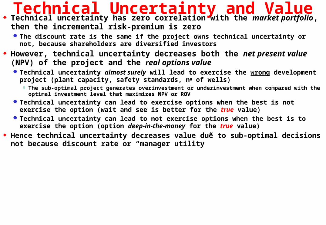
Technical Uncertainty and Value Technical uncertainty has zero correlation with the market portfolio, then the incremental

risk-premium is zero The discount rate is the same if the project owns technical uncertainty or not, because shareholders are

diversified investors However, technical uncertainty decreases both the net present value (NPV) of the project

and the real options value Technical uncertainty almost surely will lead to exercise the wrong development project (plant capacity,

safety standards, no of wells) The sub-optimal project generates overinvestment or underinvestment when compared with the optimal investment level

that maximizes NPV or ROV Technical uncertainty can lead to exercise options when the best is not exercise the option (wait and see is

better for the true value) Technical uncertainty can lead to not exercise options when the best is to exercise the option (option deep-

in-the-money for the true value) Hence technical uncertainty decreases value due to sub-optimal decisions not because discount

rate or “manager utility”

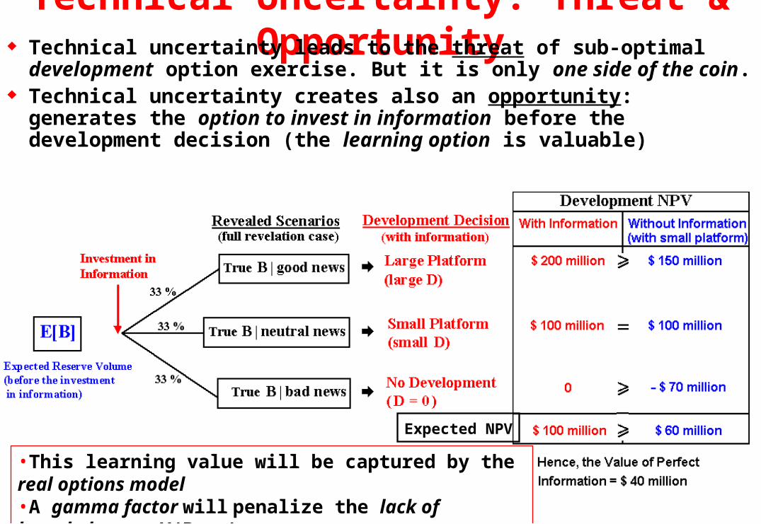
Technical Uncertainty: Threat & Opportunity Technical uncertainty leads to the threat of sub-optimal development

option exercise. But it is only one side of the coin. Technical uncertainty creates also an opportunity: generates the

option to invest in information before the development decision (the learning option is valuable)

Expected NPV

•This learning value will be captured by the real options model•A gamma factor will penalize the lack of knowledge on V(B, q)•We’ll use optimal development investment equation for D(B)

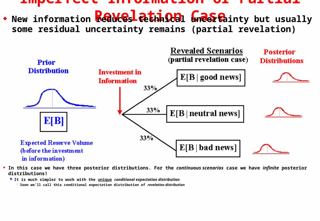
Imperfect Information or Partial Revelation Case New information reduces technical uncertainty but usually some

residual uncertainty remains (partial revelation)

In this case we have three posterior distributions. For the continuous scenarios case we have infinite posterior distributions! It is much simpler to work with the unique conditional expectation distribution

Soon we’ll call this conditional expectation distribution of revelation distribution

Conditional Expectation in Theory and Practice Let us answer assignment question 1.b on the relevance of the conditional expectation

concept for learning process valuation In the last slide we saw that is much simpler to work with the unique conditional expectation distribution

than many posterior distributions Other practical advantage: expectations has a natural place in finance

Firms use current expectations to calculate the NPV or the real options exercise payoff. Ex-ante the investment in information, the new expectation is conditional.

The price of a derivative is simply an expectation of futures values (Tavella, 2002)

The concept of conditional expectation is also theoretically sound: We want to estimate X by observing I, using a function g( I ). The most frequent measure of quality of a predictor g is its mean square error defined by MSE(g) = E[X g( I )]2 .

The choice of g* that minimizes the error measure MSE(g) is exactly the conditional expectation E[X | I ]. This is a very known property used in econometrics

Even in decision analysis literature, is common to work with conditional expectation inside the maximization equation (e.g., McCardle, 1985) But instead conditional expectation properties, the focus has been likelihood function

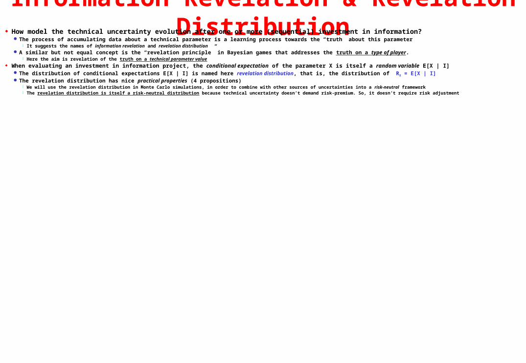
Information Revelation & Revelation Distribution How model the technical uncertainty evolution after one or more (sequential) investment in information?

The process of accumulating data about a technical parameter is a learning process towards the “truth” about this parameter It suggests the names of information revelation and revelation distribution

A similar but not equal concept is the “revelation principle” in Bayesian games that addresses the truth on a type of player. Here the aim is revelation of the truth on a technical parameter value

When evaluating an investment in information project, the conditional expectation of the parameter X is itself a random variable E[X | I] The distribution of conditional expectations E[X | I] is named here revelation distribution, that is, the distribution of RX = E[X | I] The revelation distribution has nice practical properties (4 propositions)

We will use the revelation distribution in Monte Carlo simulations, in order to combine with other sources of uncertainties into a risk-neutral framework The revelation distribution is itself a risk-neutral distribution because technical uncertainty doesn’t demand risk-premium. So, it doesn’t require risk adjustment

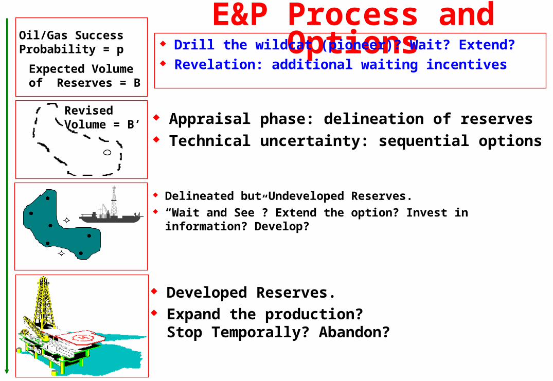
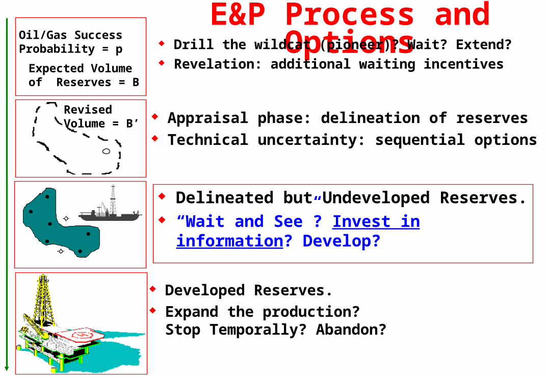
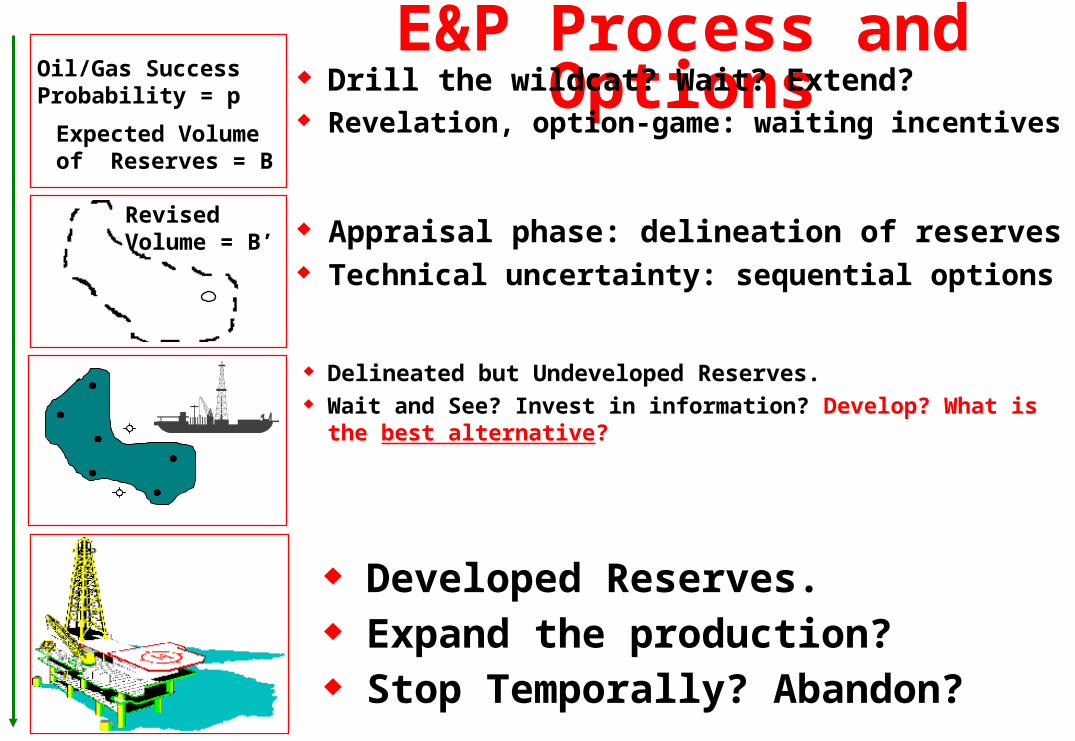
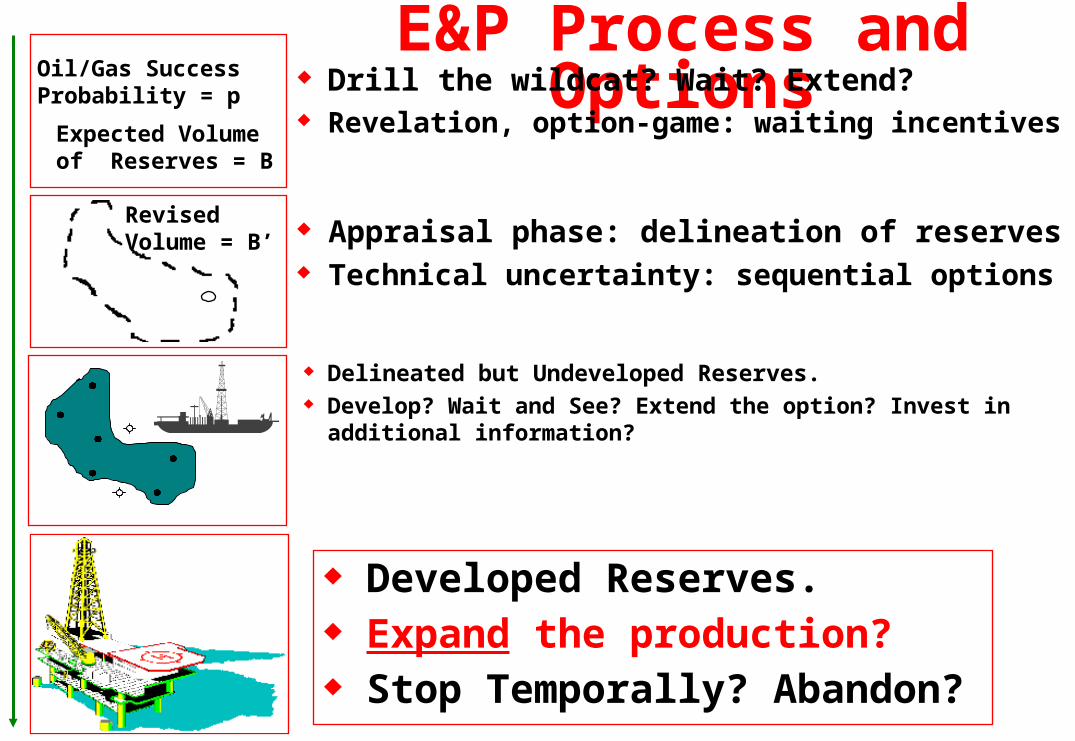
E&P Process and Options Drill the wildcat (pioneer)? Wait? Extend? Revelation: additional waiting incentives

Oil/Gas SuccessProbability = p

Expected Volumeof Reserves = B

RevisedVolume = B’ Appraisal phase: delineation of reserves

Technical uncertainty: sequential options

Delineated but Undeveloped Reserves. “Wait and See”? Extend the option? Invest in information? Develop?

Developed Reserves. Expand the production?

Stop Temporally? Abandon?

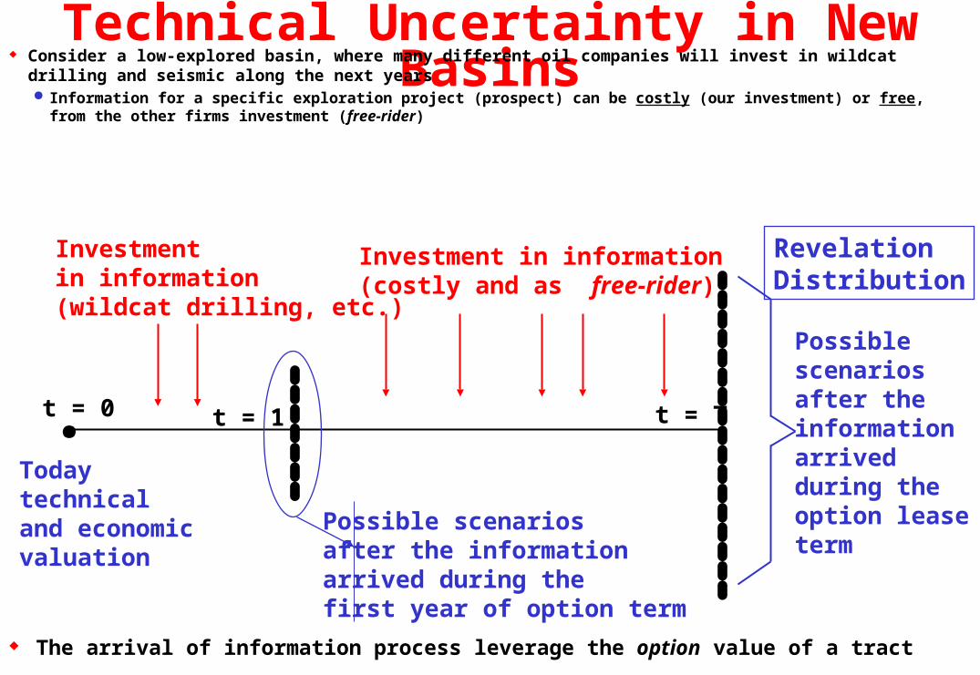
Technical Uncertainty in New Basins Consider a low-explored basin, where many different oil companies will invest in wildcat drilling and seismic along the next

years Information for a specific exploration project (prospect) can be costly (our investment) or free, from the other firms investment (free-

rider)

The arrival of information process leverage the option value of a tract

.

Investmentin information(wildcat drilling, etc.)

Investment in information(costly and as free-rider)

Todaytechnicaland economicvaluation

t = 0 t = 1

Possible scenariosafter the informationarrived during the first year of option term

t = T

Possible scenariosafter the informationarrived during the option leaseterm

RevelationDistribution

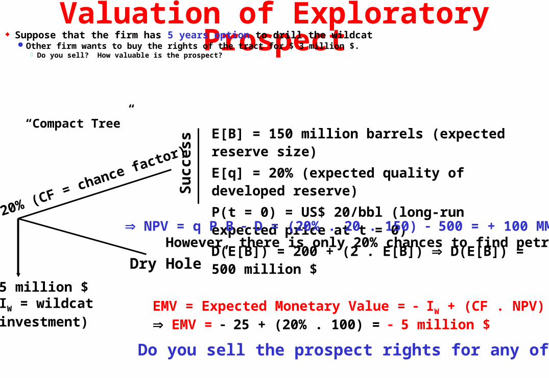
Valuation of Exploratory Prospect Suppose that the firm has 5 years option to drill the wildcat

Other firm wants to buy the rights of the tract for $ 3 million $. Do you sell? How valuable is the prospect?

E[B] = 150 million barrels (expected reserve size)

E[q] = 20% (expected quality of developed reserve)

P(t = 0) = US$ 20/bbl (long-run expected price at t = 0)

D(E[B]) = 200 + (2 . E[B]) D(E[B]) = 500 million $

NPV = q P B D = (20% . 20 . 150) 500 = + 100 MM$ However, there is only 20% chances to find petroleum

EMV = Expected Monetary Value = IW + (CF . NPV) EMV = 25 + (20% . 100) = 5 million $

25 million $(IW = wildcat investment)

20% (CF = chance factor)

Dry Hole

“Compact Tree”

Su

cces

s

Do you sell the prospect rights for any offer?

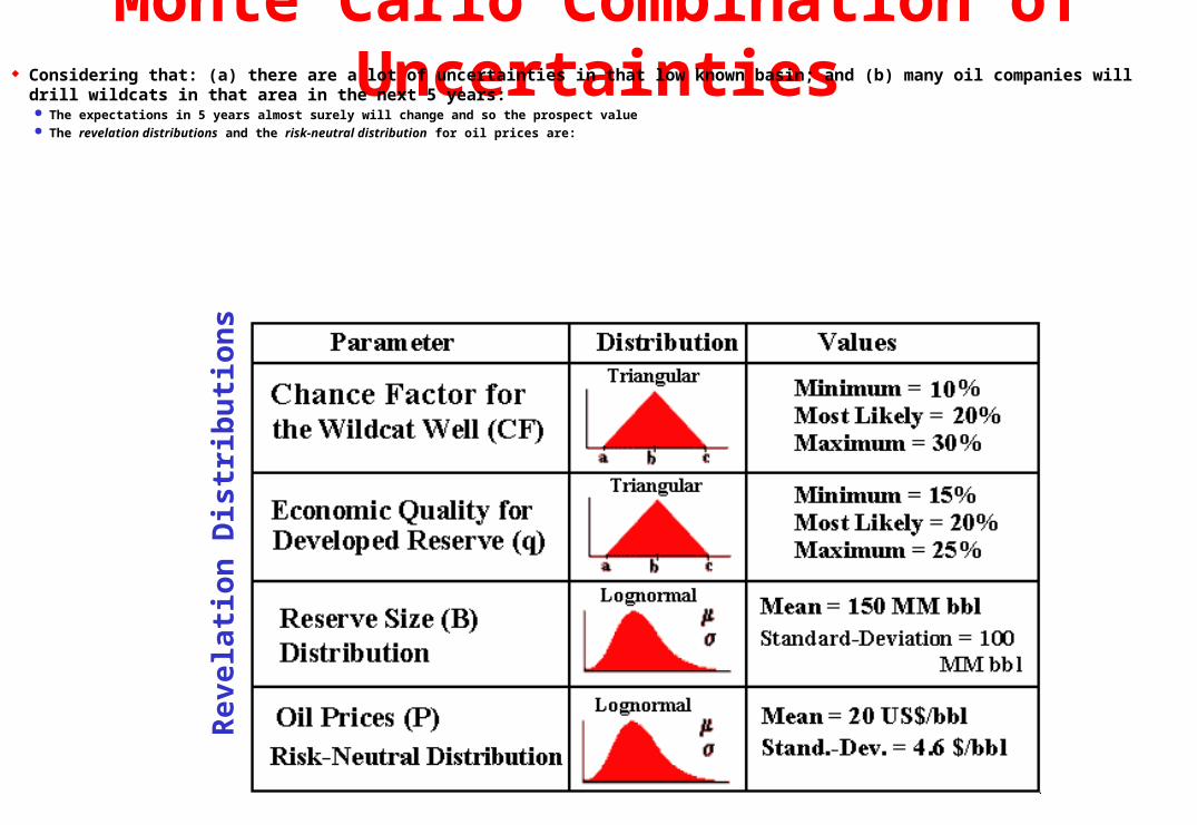
Monte Carlo Combination of Uncertainties Considering that: (a) there are a lot of uncertainties in that low known basin; and (b) many oil companies will drill wildcats in that area in the next 5

years: The expectations in 5 years almost surely will change and so the prospect value The revelation distributions and the risk-neutral distribution for oil prices are:

Rev

elat

ion

Dis

trib

uti

ons

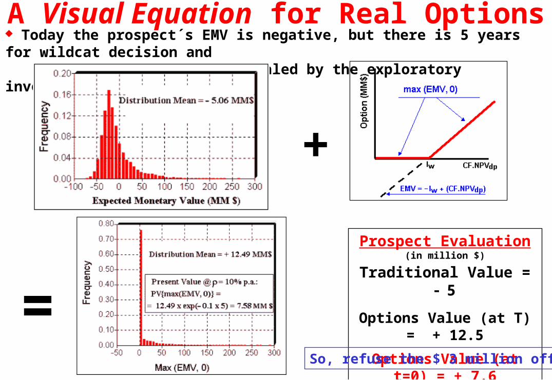
A Visual Equation for Real Options

Prospect Evaluation(in million $)

Traditional Value = 5

Options Value (at T) = + 12.5

Options Value (at t=0) = + 7.6

+

Today the prospect´s EMV is negative, but there is 5 years for wildcat decision and new scenarios will be revealed by the exploratory investment in that basin.

=So, refuse the $ 3 million offer!

E&P Process and Options Drill the wildcat (pioneer)? Wait? Extend? Revelation: additional waiting incentives

Oil/Gas SuccessProbability = p

Expected Volumeof Reserves = B

RevisedVolume = B’ Appraisal phase: delineation of reserves

Technical uncertainty: sequential options

Delineated but Undeveloped Reserves. “Wait and See”? Invest in information?

Develop?

Developed Reserves. Expand the production?

Stop Temporally? Abandon?

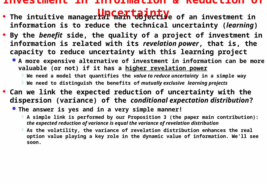
Investment in Information & Reduction of Uncertainty The intuitive managerial main objective of an investment in information is to

reduce the technical uncertainty (learning) By the benefit side, the quality of a project of investment in information is

related with its revelation power, that is, the capacity to reduce uncertainty with this learning project A more expensive alternative of investment in information can be more valuable (or

not) if it has a higher revelation power We need a model that quantifies the value to reduce uncertainty in a simple way We need to distinguish the benefits of mutually exclusive learning projects

Can we link the expected reduction of uncertainty with the dispersion (variance) of the conditional expectation distribution? The answer is yes and in a very simple manner!

A simple link is performed by our Proposition 3 (the paper main contribution): the expected reduction of variance is equal the variance of revelation distribution

As the volatility, the variance of revelation distribution enhances the real option value playing a key role in the dynamic value of information. We’ll see soon.

The Revelation Distribution Properties Full revelation definition: when new information reveal all the truth about a technical parameter X, we have full revelation

Much more common is the partial revelation case, but full revelation is important as the limit goal for any investment in information process The revelation distributions RX (or conditional expectations distributions) have at least 4 nice properties for modeling:

Proposition 1: for the full revelation case, the distribution of revelation RX is equal to the prior (unconditional) distribution of X (RX in the limit) Proposition 2: The expected value for the revelation distribution is equal the expected value of the original (prior) distribution

That is: E[E[X | I ]] = E[RX] = E[X] (known as law of iterated expectations) Proposition 3: the variance of the revelation distribution is equal to the expected reduction of variance induced by the new information

Var[E[X | I ]] = Var[RX] = Var[X] E[Var[X | I ]] = Expected Variance Reduction (this property reports the revelation power of a learning project) Proposition 4: In a sequential investment process, the ex-ante sequential revelation distributions {RX,1, RX,2, RX,3, …} are (event-driven) martingales

In short, ex-ante these random variables have the same mean

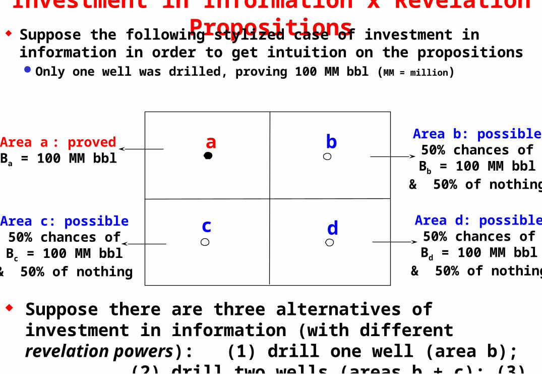
Investment in Information x Revelation Propositions Suppose the following stylized case of investment in information in order to get

intuition on the propositions Only one well was drilled, proving 100 MM bbl (MM = million)

a b

dc

Area a : provedBa = 100 MM bbl

Area b: possible50% chances of

Bb = 100 MM bbl& 50% of nothing

Area d: possible50% chances of

Bd = 100 MM bbl& 50% of nothing

Area c: possible50% chances of

Bc = 100 MM bbl& 50% of nothing

Suppose there are three alternatives of investment in information (with different revelation powers): (1) drill one well (area b); (2) drill two wells (areas b + c); (3) drill three wells (b + c + d)

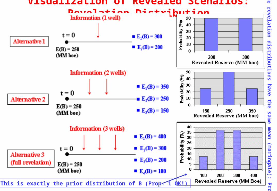
Visualization of Revealed Scenarios: Revelation Distribution

This is exactly the prior distribution of B (Prop. 1 OK!)

All th

e revelation d

istribu

tions h

ave the sam

e mean

(marin

gale): Prop

. 4 OK

!

Distributions of conditional expectations

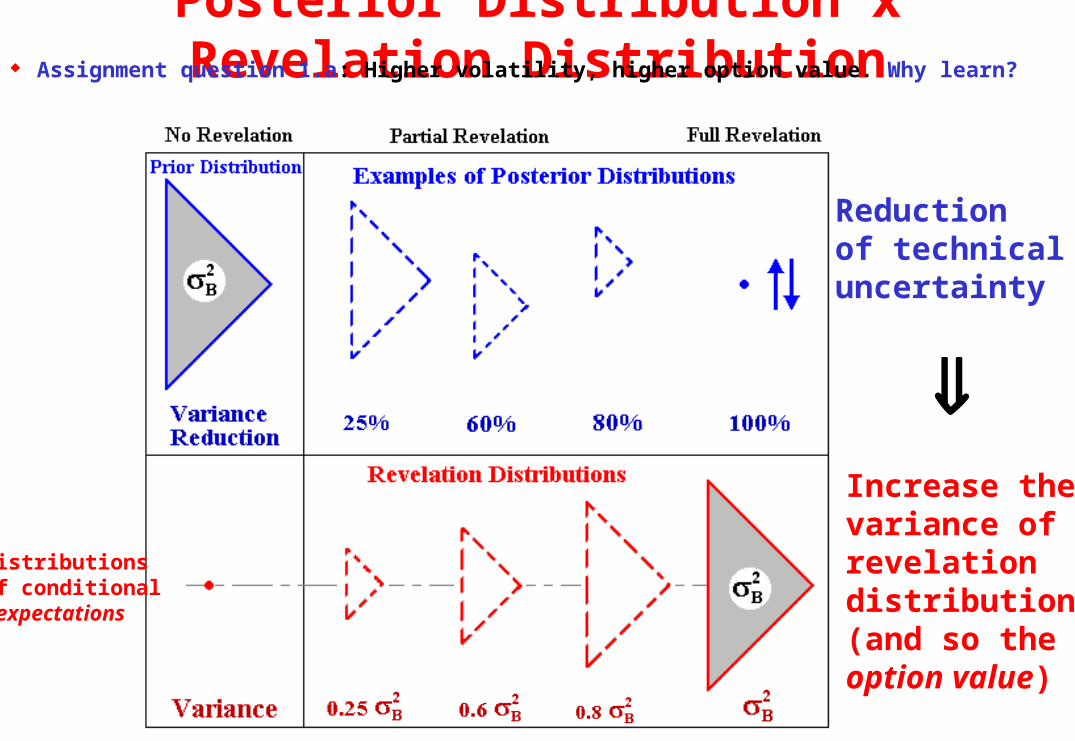
Posterior Distribution x Revelation Distribution Assignment question 1.a: Higher volatility, higher option value. Why learn?

Reduction of technical uncertainty

Increase thevariance ofrevelationdistribution(and so the option value)

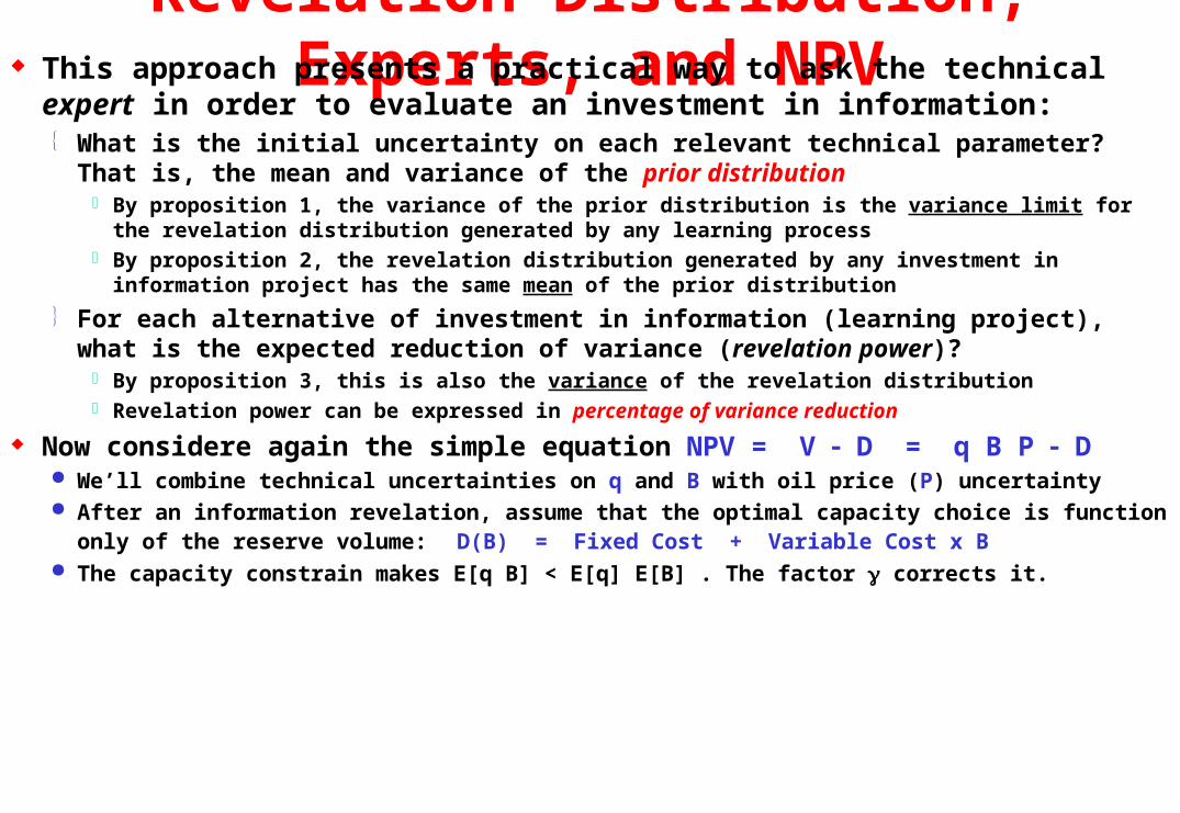
Revelation Distribution, Experts, and NPV This approach presents a practical way to ask the technical expert in order

to evaluate an investment in information: What is the initial uncertainty on each relevant technical parameter? That is, the mean

and variance of the prior distribution By proposition 1, the variance of the prior distribution is the variance limit for the revelation

distribution generated by any learning process By proposition 2, the revelation distribution generated by any investment in information project has

the same mean of the prior distribution

For each alternative of investment in information (learning project), what is the expected reduction of variance (revelation power)? By proposition 3, this is also the variance of the revelation distribution Revelation power can be expressed in percentage of variance reduction

Now considere again the simple equation NPV = V D = q B P D We’ll combine technical uncertainties on q and B with oil price (P) uncertainty After an information revelation, assume that the optimal capacity choice is function only of the

reserve volume: D(B) = Fixed Cost + Variable Cost x B The capacity constrain makes E[q B] < E[q] E[B] . The factor corrects it.

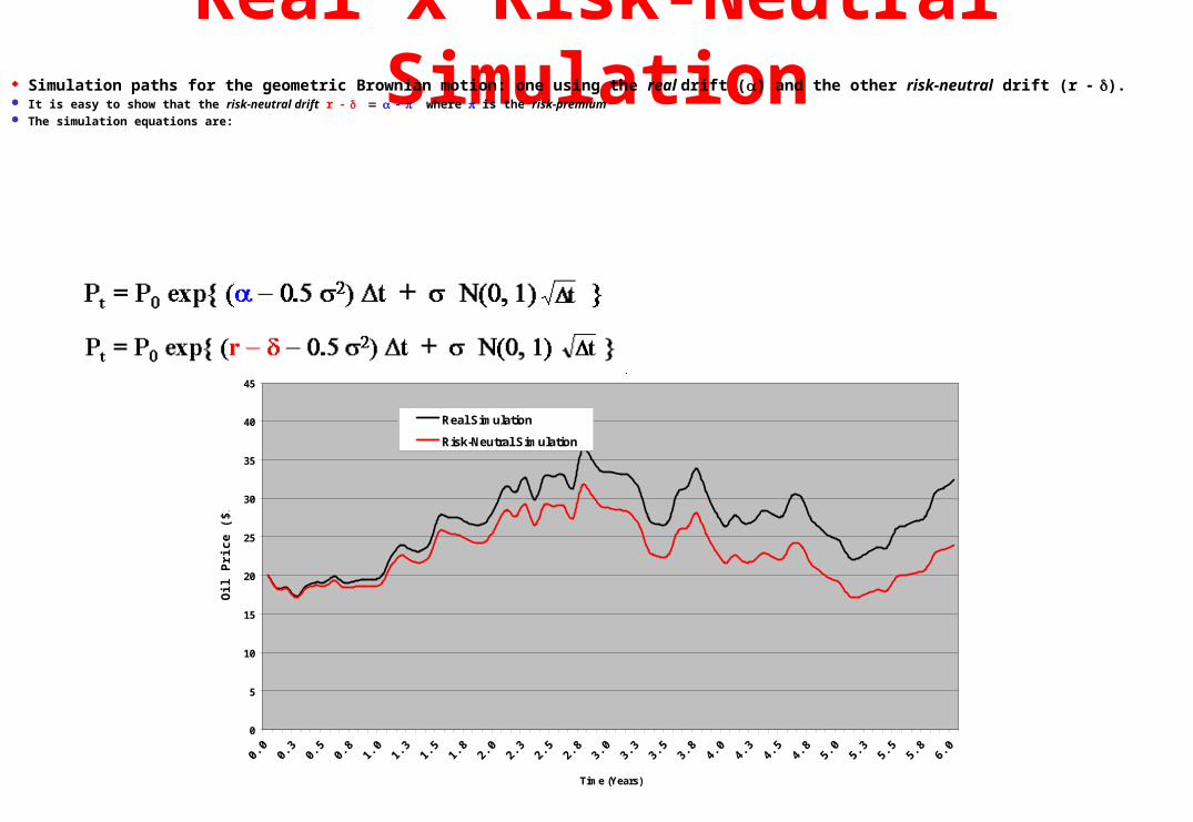
Real x Risk-Neutral Simulation Simulation paths for the geometric Brownian motion: one using the real drift () and the other risk-neutral drift (r ). It is easy to show that the risk-neutral drift r where is the risk-premium The simulation equations are:

0

5

10

15

20

25

30

35

40

45

0.0

0.3

0.5

0.8

1.0

1.3

1.5

1.8

2.0

2.3

2.5

2.8

3.0

3.3

3.5

3.8

4.0

4.3

4.5

4.8

5.0

5.3

5.5

5.8

6.0

Time (Years)

Oil

Pri

ce ($

/bb

l)

Real Simulation

Risk-Neutral Simulation

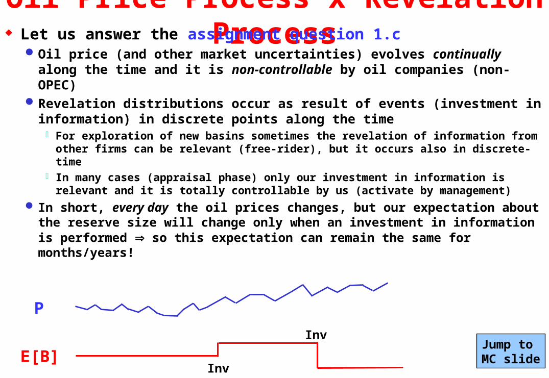
Oil Price Process x Revelation Process Let us answer the assignment question 1.c

Oil price (and other market uncertainties) evolves continually along the time and it is non-controllable by oil companies (non-OPEC)

Revelation distributions occur as result of events (investment in information) in discrete points along the time For exploration of new basins sometimes the revelation of information from other

firms can be relevant (free-rider), but it occurs also in discrete-time In many cases (appraisal phase) only our investment in information is relevant and

it is totally controllable by us (activate by management)

In short, every day the oil prices changes, but our expectation about the reserve size will change only when an investment in information is performed so this expectation can remain the same for months/years!

P

E[B]Inv

InvJump to MC slide

The Normalized Threshold and Valuation Assignment question 1.d is about valuation under optimization Recall that the development option is optimally exercised at the

threshold V*, when V is suficiently higher than D Exercise the option only if the project is “deep-in-the-money”

Assume the optimal investment D as a linear function of B and independent of q: D(B) = 310 + 2.1 x B (in millions $)

This means that if B varies, the exercise price D of our option also varies, and so the threshold V*. Relevant computational time to calculate V* for different values of D

We need perform a Monte Carlo simulation to combine the uncertainties after an information revelation. After each B sampling, it is necessary to calculate the new threshold curve V*(t) to

see if the project value V = q P B is deep-in-the money In order to reduce the computational time, we work with the normalized

threshold (V/D)*. Why?

Normalized Threshold and Valuation We will perform the valuation considering the optimal exercise at the

normalized threshold level (V/D)* After each Monte Carlo simulation combining the revelation distributions of q and B

with the risk-neutral simulation of P We calculate V = q P B and D(B), so V/D, and compare with (V/D)*

Advantage: (V/D)* is homogeneous of degree 0 in V and D. This means that the rule (V/D)* remains valid for any V and D So, for any revealed scenario of B, changing D, the rule (V/D)* holds This was proved only for geometric Brownian motion (V/D)*(t) changes only if the risk-neutral stochastic process parameters r, , change.

But these factors don’t change at Monte Carlo simulation

The computational time of using (V/D)* is much lower than V* The vector (V/D)*(t) is calculated only once, whereas V*(t) needs be re-calculated

every iteration in the Monte Carlo simulation. V* is a time-consuming calculus

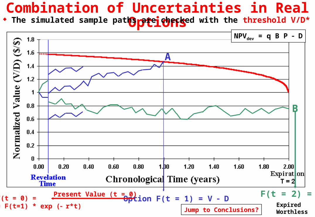
Combination of Uncertainties in Real Options The simulated sample paths are checked with the threshold V/D*

A

Option F(t = 1) = V DF(t = 0) == F(t=1) * exp (r*t)

Present Value (t = 0)

B

F(t = 2) = 0ExpiredWorthless

NPVdev = q B P D

Jump to Conclusions?

Best Alternative of Investment in Information

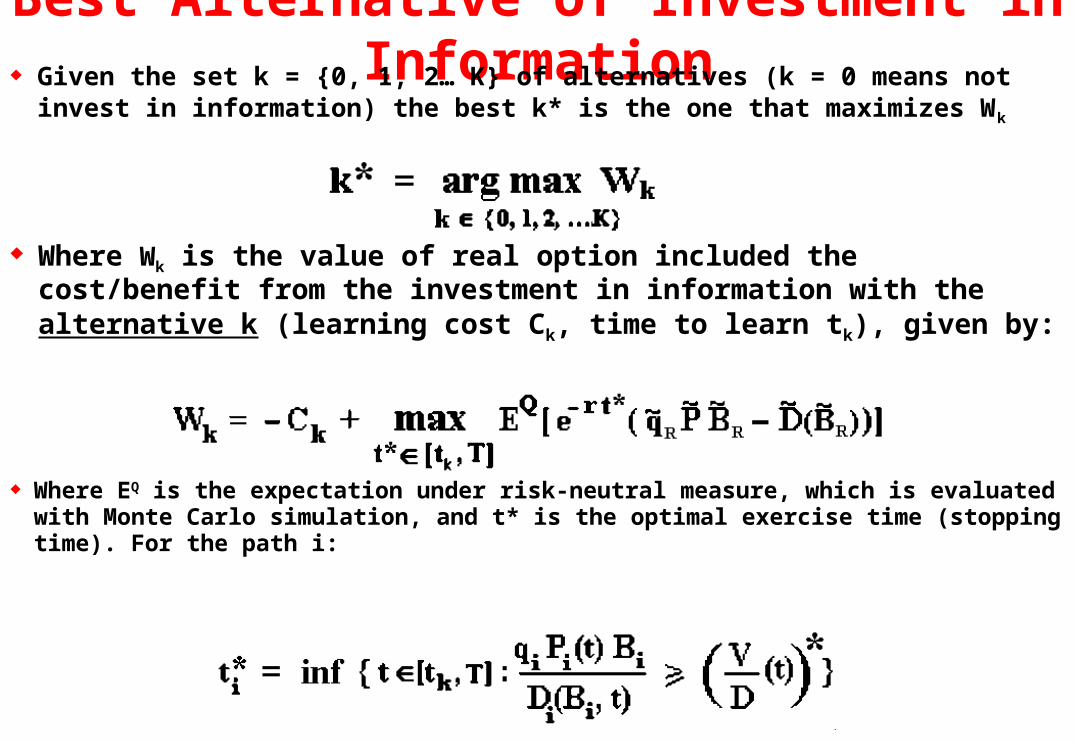
Where Wk is the value of real option included the cost/benefit from the investment in information with the alternative k (learning cost Ck, time to learn tk), given by:

Where EQ is the expectation under risk-neutral measure, which is evaluated with Monte Carlo simulation, and t* is the optimal exercise time (stopping time). For the path i:

Given the set k = {0, 1, 2… K} of alternatives (k = 0 means not invest in information) the best k* is the one that maximizes Wk

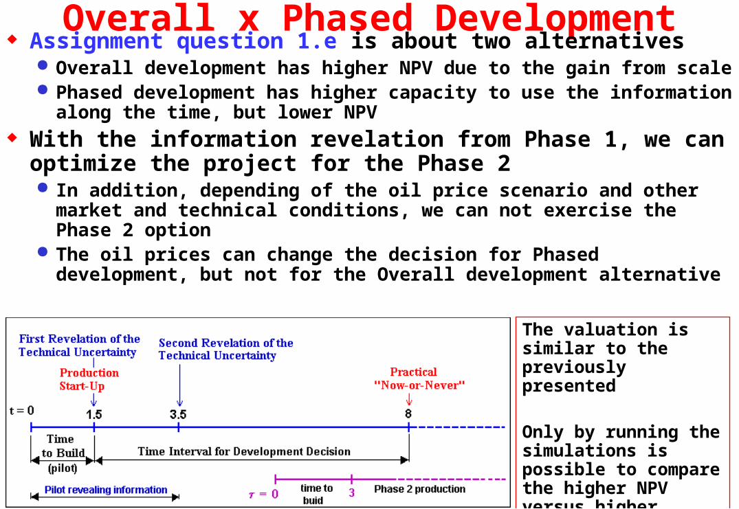
Overall x Phased Development Assignment question 1.e is about two alternatives

Overall development has higher NPV due to the gain from scale Phased development has higher capacity to use the information along

the time, but lower NPV With the information revelation from Phase 1, we can

optimize the project for the Phase 2 In addition, depending of the oil price scenario and other market and

technical conditions, we can not exercise the Phase 2 option The oil prices can change the decision for Phased development, but not

for the Overall development alternativeThe valuation is similar to the previously presented

Only by running the simulations is possible to compare the higher NPV versus higher flexibility

Spreadsheet Application Assignment Part 2 Let us see the spreadsheet timing_inv_inf-hqr.xls It permits to choose the best alternative of investment in

information (and check if is better to invest in information or not)

It calculates the dynamic net value of information

timing_inv_inf-hqr.xls

E&P Process and Options Drill the wildcat? Wait? Extend? Revelation, option-game: waiting incentives

Oil/Gas SuccessProbability = p

Expected Volumeof Reserves = B

RevisedVolume = B’ Appraisal phase: delineation of reserves

Technical uncertainty: sequential options

Developed Reserves. Expand the production? Stop Temporally? Abandon?

Delineated but Undeveloped Reserves. Wait and See? Invest in information? Develop? What is the best

alternative?

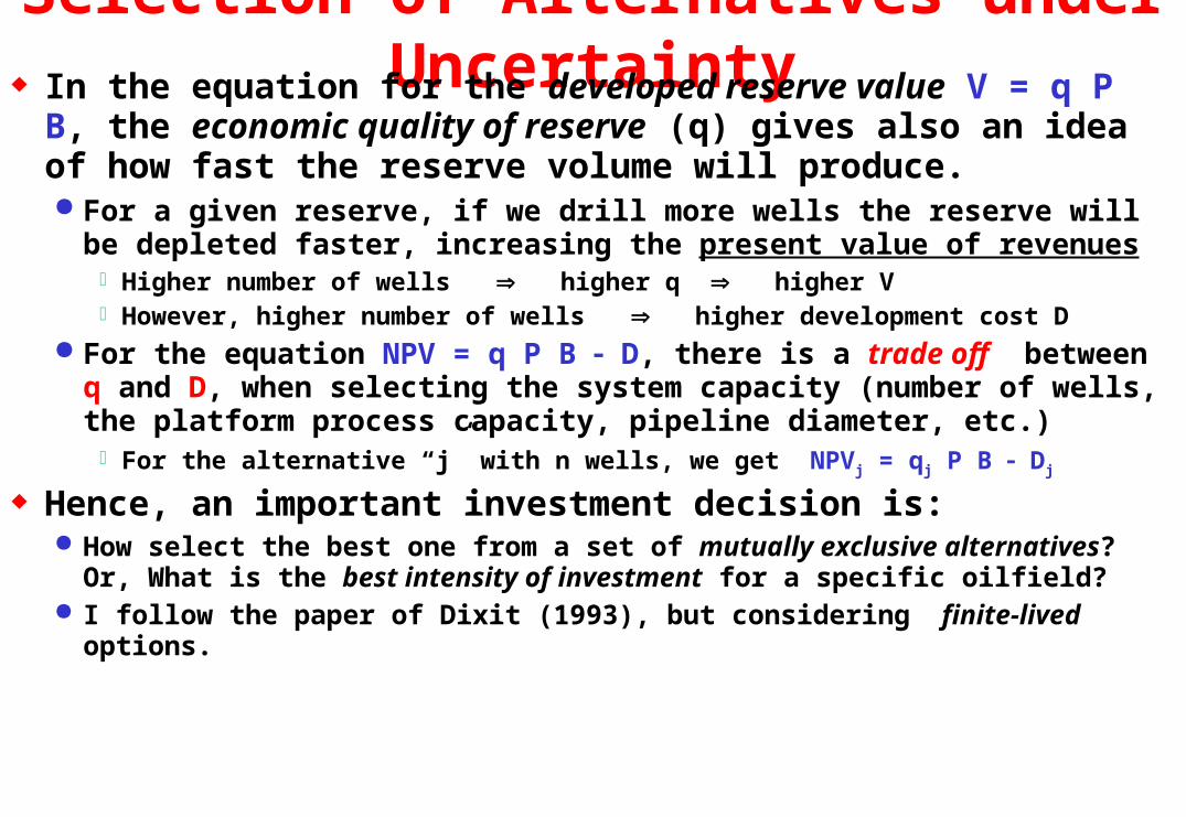
Selection of Alternatives under Uncertainty In the equation for the developed reserve value V = q P B, the

economic quality of reserve (q) gives also an idea of how fast the reserve volume will produce. For a given reserve, if we drill more wells the reserve will be depleted faster,

increasing the present value of revenues Higher number of wells higher q higher V However, higher number of wells higher development cost D

For the equation NPV = q P B D, there is a trade off between q and D, when selecting the system capacity (number of wells, the platform process capacity, pipeline diameter, etc.) For the alternative “j” with n wells, we get NPVj = qj P B Dj

Hence, an important investment decision is: How select the best one from a set of mutually exclusive alternatives? Or, What is the

best intensity of investment for a specific oilfield? I follow the paper of Dixit (1993), but considering finite-lived options.

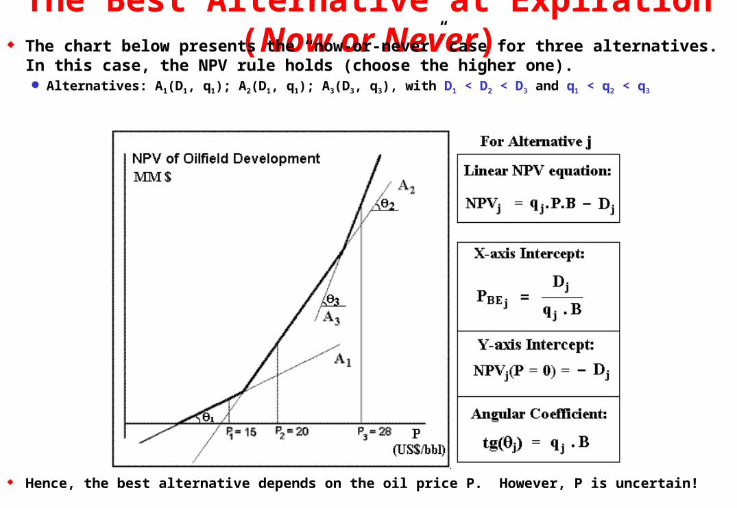
The Best Alternative at Expiration (Now or Never) The chart below presents the “now-or-never” case for three alternatives. In this case, the NPV

rule holds (choose the higher one). Alternatives: A1(D1, q1); A2(D1, q1); A3(D3, q3), with D1 < D2 < D3 and q1 < q2 < q3

Hence, the best alternative depends on the oil price P. However, P is uncertain!

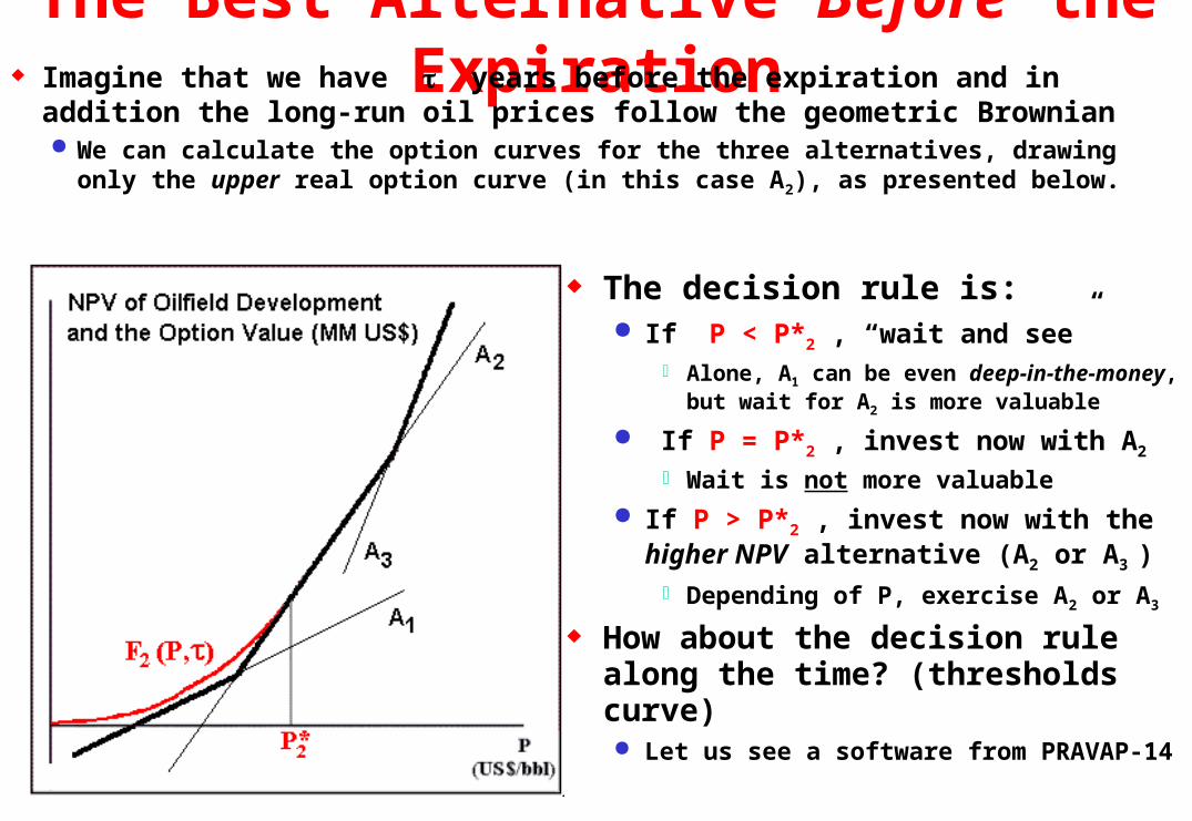
The Best Alternative Before the Expiration Imagine that we have years before the expiration and in addition

the long-run oil prices follow the geometric Brownian We can calculate the option curves for the three alternatives, drawing only

the upper real option curve (in this case A2), as presented below.

The decision rule is: If P < P*2 , “wait and see”

Alone, A1 can be even deep-in-the-money, but wait for A2 is more valuable

If P = P*2 , invest now with A2

Wait is not more valuable

If P > P*2 , invest now with the higher NPV alternative (A2 or A3 ) Depending of P, exercise A2 or A3

How about the decision rule along the time? (thresholds curve) Let us see a software from PRAVAP-14

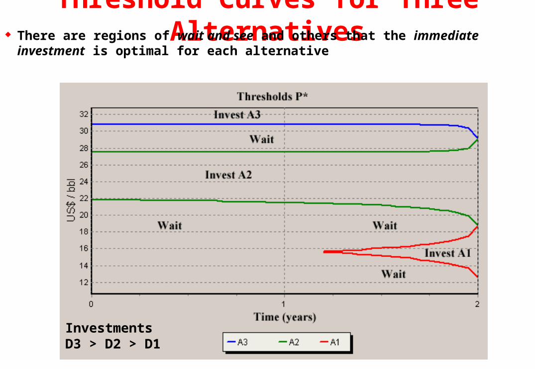
Threshold Curves for Three Alternatives There are regions of wait and see and others that the immediate investment is optimal for

each alternative

InvestmentsD3 > D2 > D1

E&P Process and Options Drill the wildcat? Wait? Extend? Revelation, option-game: waiting incentives

Oil/Gas SuccessProbability = p

Expected Volumeof Reserves = B

RevisedVolume = B’ Appraisal phase: delineation of reserves

Technical uncertainty: sequential options

Developed Reserves. Expand the production? Stop Temporally? Abandon?

Delineated but Undeveloped Reserves. Develop? Wait and See? Extend the option? Invest in additional

information?

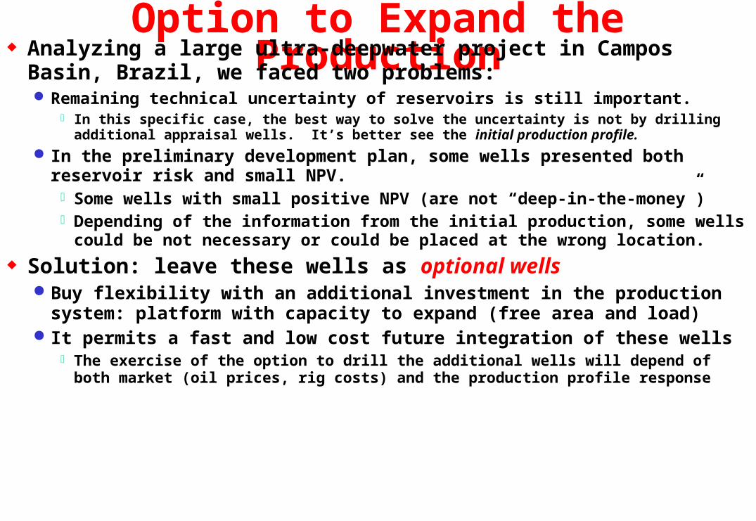
Option to Expand the Production Analyzing a large ultra-deepwater project in Campos Basin, Brazil, we

faced two problems: Remaining technical uncertainty of reservoirs is still important.

In this specific case, the best way to solve the uncertainty is not by drilling additional appraisal wells. It’s better see the initial production profile.

In the preliminary development plan, some wells presented both reservoir risk and small NPV. Some wells with small positive NPV (are not “deep-in-the-money”)Depending of the information from the initial production, some wells could be not

necessary or could be placed at the wrong location.

Solution: leave these wells as optional wells Buy flexibility with an additional investment in the production system: platform

with capacity to expand (free area and load) It permits a fast and low cost future integration of these wells

The exercise of the option to drill the additional wells will depend of both market (oil prices, rig costs) and the production profile response

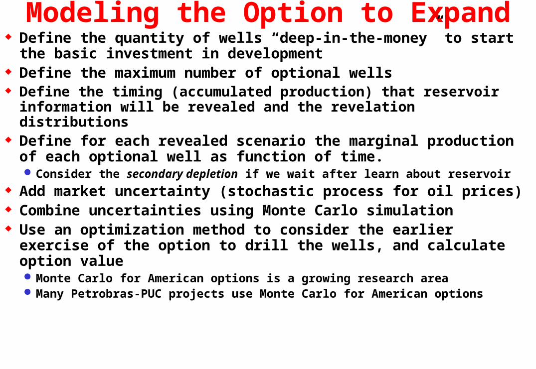
Modeling the Option to Expand Define the quantity of wells “deep-in-the-money” to start the basic

investment in development Define the maximum number of optional wells Define the timing (accumulated production) that reservoir

information will be revealed and the revelation distributions Define for each revealed scenario the marginal production of each

optional well as function of time. Consider the secondary depletion if we wait after learn about reservoir

Add market uncertainty (stochastic process for oil prices) Combine uncertainties using Monte Carlo simulation Use an optimization method to consider the earlier exercise of the

option to drill the wells, and calculate option value Monte Carlo for American options is a growing research area Many Petrobras-PUC projects use Monte Carlo for American options

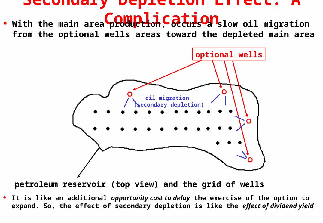
petroleum reservoir (top view) and the grid of wells

Secondary Depletion Effect: A Complication With the main area production, occurs a slow oil migration from the optional

wells areas toward the depleted main area

optional wells

oil migration (secondary depletion)

It is like an additional opportunity cost to delay the exercise of the option to expand. So, the effect of secondary depletion is like the effect of dividend yield

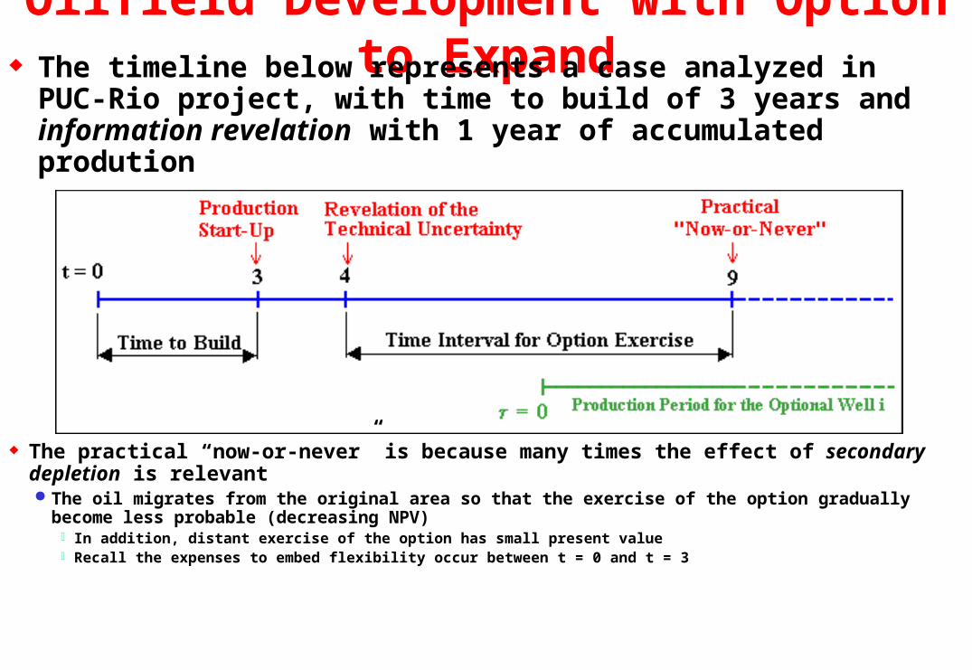
Oilfield Development with Option to Expand The timeline below represents a case analyzed in PUC-Rio

project, with time to build of 3 years and information revelation with 1 year of accumulated prodution

The practical “now-or-never” is because many times the effect of secondary depletion is relevant The oil migrates from the original area so that the exercise of the option gradually become less probable

(decreasing NPV) In addition, distant exercise of the option has small present value Recall the expenses to embed flexibility occur between t = 0 and t = 3

Conclusions The real options models in petroleum bring a rich framework to

consider optimal investment under uncertainty, recognizing the managerial flexibilities Traditional discounted cash flow (DCF) is very limited and can induce to

serious errors in negotiations and decisions We saw the classical model, working with the intuition and real

options toolkit We see different stochastic processes and other models

I gave an idea about the real options research at Petrobras and PUC-Rio

We worked more in models of value of information combining technical uncertainties with market uncertainty The model using the revelation distribution gives the correct incentives for

investment in information Thank you very much for your time

Anexos

APPENDIXSUPPORT SLIDES

See more on real options in the first website on real options at: http://www.puc-rio.br/marco.ind/

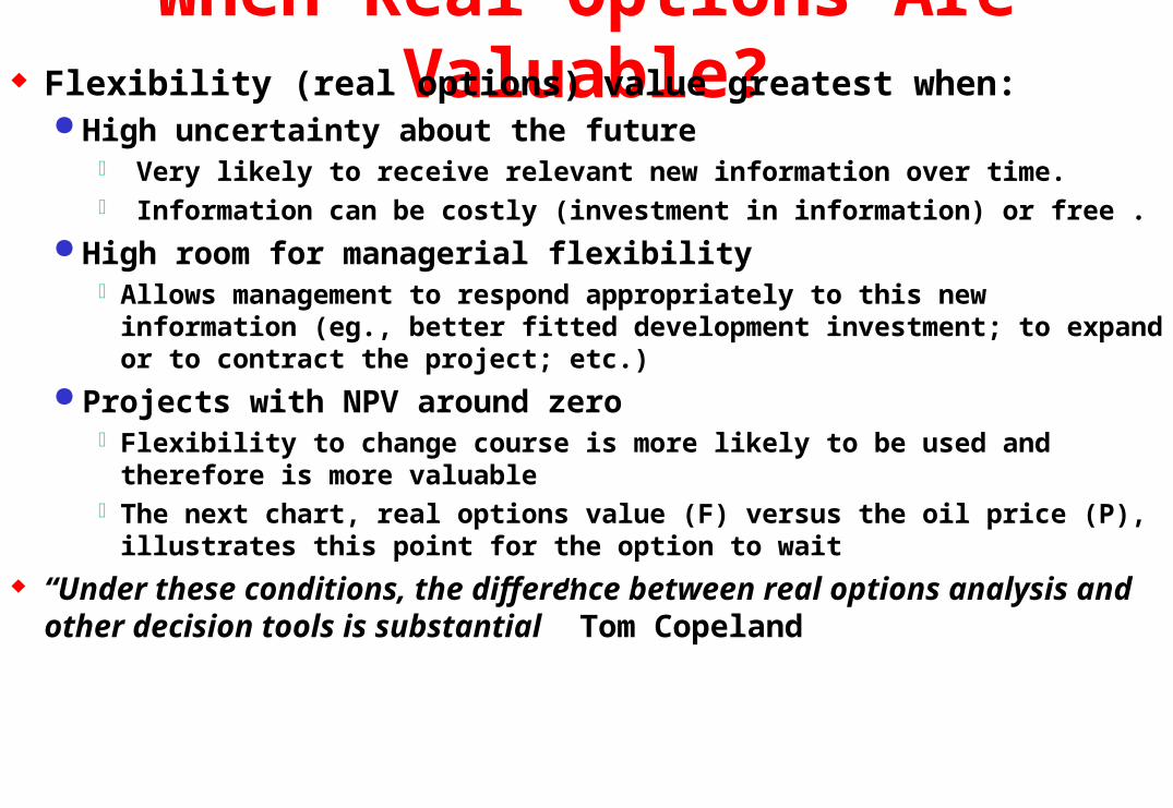
When Real Options Are Valuable? Flexibility (real options) value greatest when:

High uncertainty about the future Very likely to receive relevant new information over time. Information can be costly (investment in information) or free .

High room for managerial flexibilityAllows management to respond appropriately to this new information (eg., better

fitted development investment; to expand or to contract the project; etc.)

Projects with NPV around zero Flexibility to change course is more likely to be used and therefore is more

valuable The next chart, real options value (F) versus the oil price (P), illustrates this point

for the option to wait

“Under these conditions, the difference between real options analysis and other decision tools is substantial” Tom Copeland

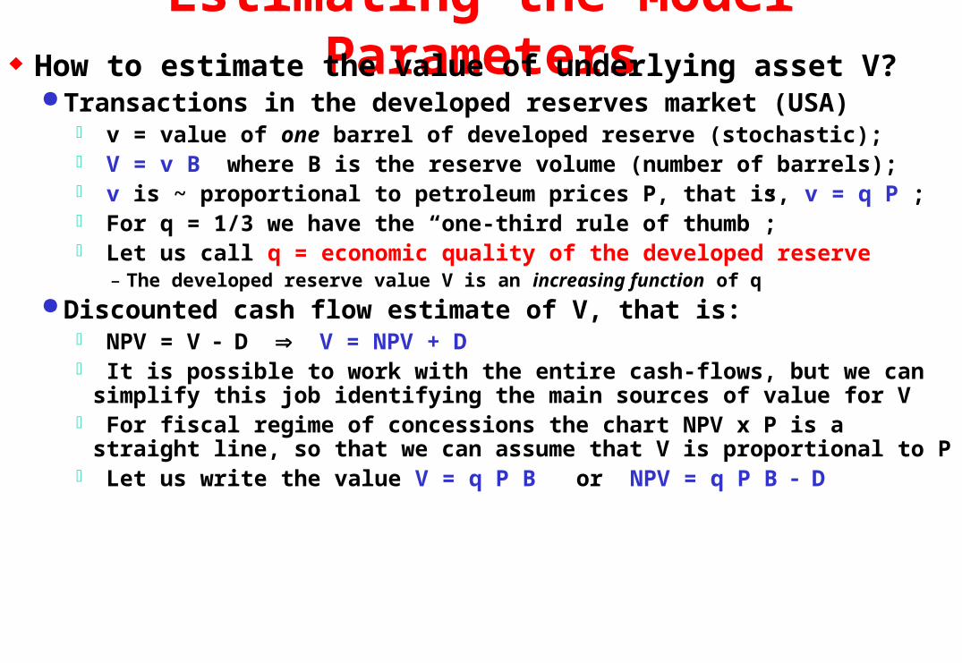
Estimating the Model Parameters How to estimate the value of underlying asset V?

Transactions in the developed reserves market (USA) v = value of one barrel of developed reserve (stochastic); V = v B where B is the reserve volume (number of barrels); v is ~ proportional to petroleum prices P, that is, v = q P ; For q = 1/3 we have the “one-third rule of thumb”; Let us call q = economic quality of the developed reserve

– The developed reserve value V is an increasing function of q

Discounted cash flow estimate of V, that is: NPV = V D V = NPV + D It is possible to work with the entire cash-flows, but we can simplify this job

identifying the main sources of value for V For fiscal regime of concessions the chart NPV x P is a straight line, so that

we can assume that V is proportional to P Let us write the value V = q P B or NPV = q P B D

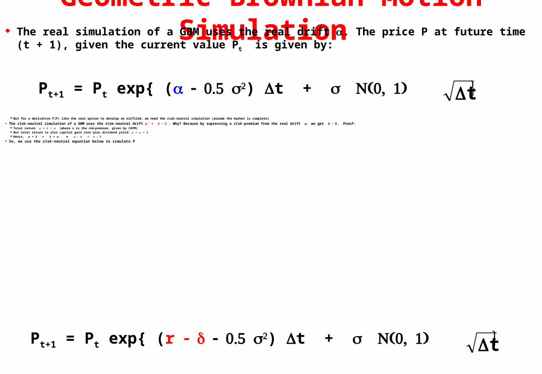
Geometric Brownian Motion Simulation The real simulation of a GBM uses the real drift . The price P at future time (t + 1), given the current

value Pt is given by:

Pt+1 = Pt exp{ () t + t But for a derivative F(P) like the real option to develop an oilfiled, we need the risk-neutral simulation (assume the market is complete)

The risk-neutral simulation of a GBM uses the risk-neutral drift ’ = r . Why? Because by supressing a risk-premium from the real drift we get r . Proof: Total return = r + (where is the risk-premium, given by CAPM) But total return is also capital gain rate plus dividend yield: = + Hence, + r + = r

So, we use the risk-neutral equation below to simulate P

Pt+1 = Pt exp{ (r ) t + t

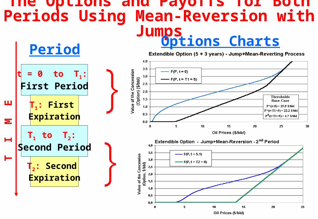
The Options and Payoffs for Both Periods Using Mean-Reversion with Jumps

T I

M E

Options Charts

T2: Second Expiration

t = 0 to T1:

First Period

T1: First Expiration

T1 to T2:

Second Period

Period

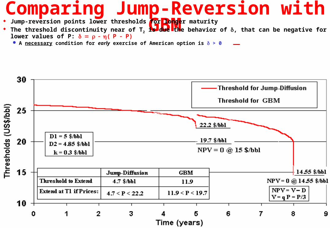
Comparing Jump-Reversion with GBM Jump-reversion points lower thresholds for longer maturity The threshold discontinuity near of T2 is due the behavior of , that can be negative for lower values of P:

( P P) A necessary condition for early exercise of American option is > 0

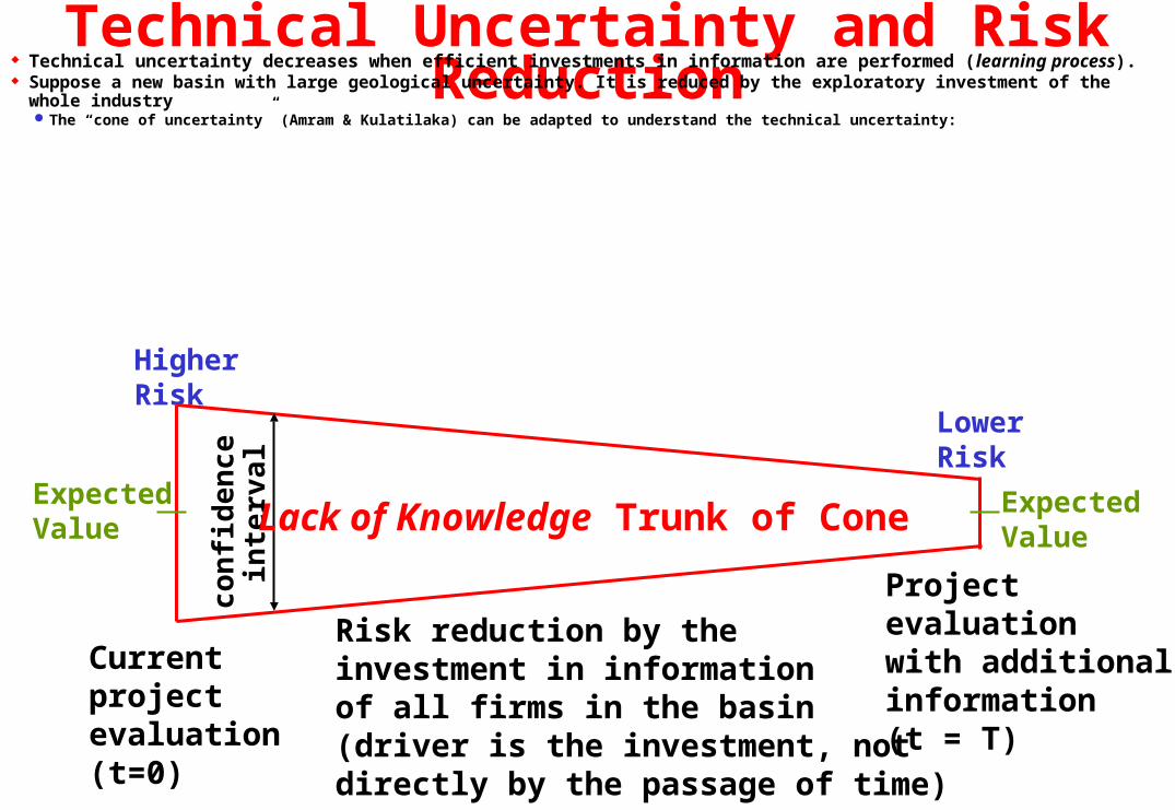
Technical Uncertainty and Risk Reduction Technical uncertainty decreases when efficient investments in information are performed ( learning process). Suppose a new basin with large geological uncertainty. It is reduced by the exploratory investment of the whole industry

The “cone of uncertainty” (Amram & Kulatilaka) can be adapted to understand the technical uncertainty:

Risk reduction by the investment in information of all firms in the basin(driver is the investment, not directly by the passage of time)

Project evaluation with additionalinformation(t = T)

Lower Risk

ExpectedValue

Current project evaluation(t=0)

HigherRisk

ExpectedValue

con

fid

ence

in

terv

al

Lack of Knowledge Trunk of Cone

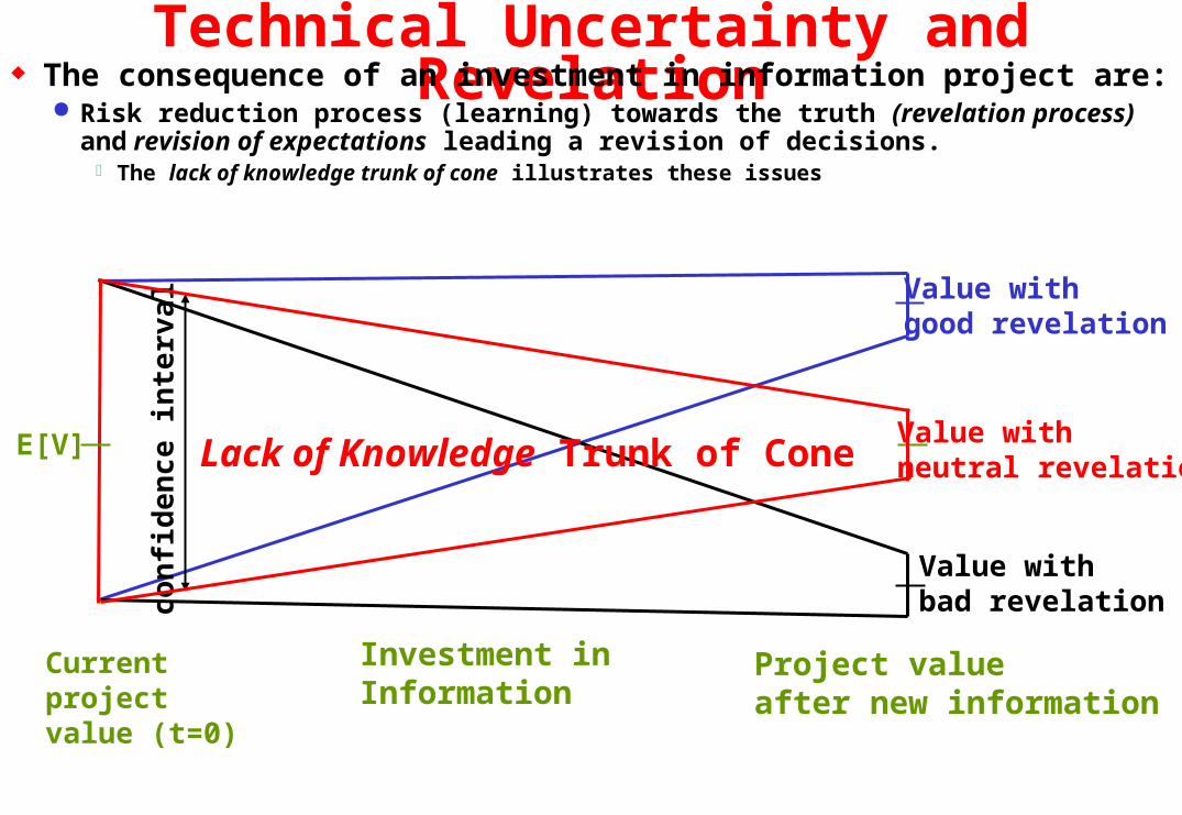
Technical Uncertainty and Revelation The consequence of an investment in information project are:

Risk reduction process (learning) towards the truth (revelation process) and revision of expectations leading a revision of decisions. The lack of knowledge trunk of cone illustrates these issues

Value withgood revelation

Value withbad revelation

con

fid

ence

inte

rval

Current project value (t=0)

Investment inInformation

Project valueafter new information

Value withneutral revelation

E[V] Lack of Knowledge Trunk of Cone

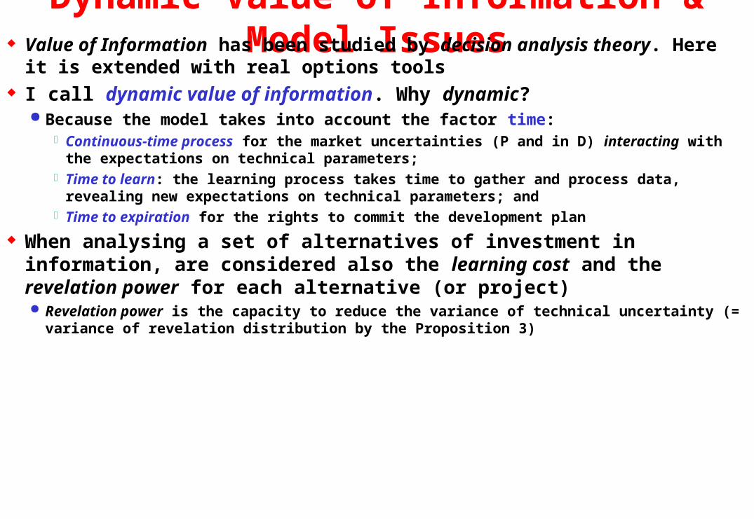
Dynamic Value of Information & Model Issues Value of Information has been studied by decision analysis theory. Here it is

extended with real options tools I call dynamic value of information. Why dynamic?

Because the model takes into account the factor time:Continuous-time process for the market uncertainties (P and in D) interacting with the expectations on

technical parameters; Time to learn: the learning process takes time to gather and process data, revealing new expectations

on technical parameters; andTime to expiration for the rights to commit the development plan

When analysing a set of alternatives of investment in information, are considered also the learning cost and the revelation power for each alternative (or project) Revelation power is the capacity to reduce the variance of technical uncertainty (= variance of revelation

distribution by the Proposition 3)

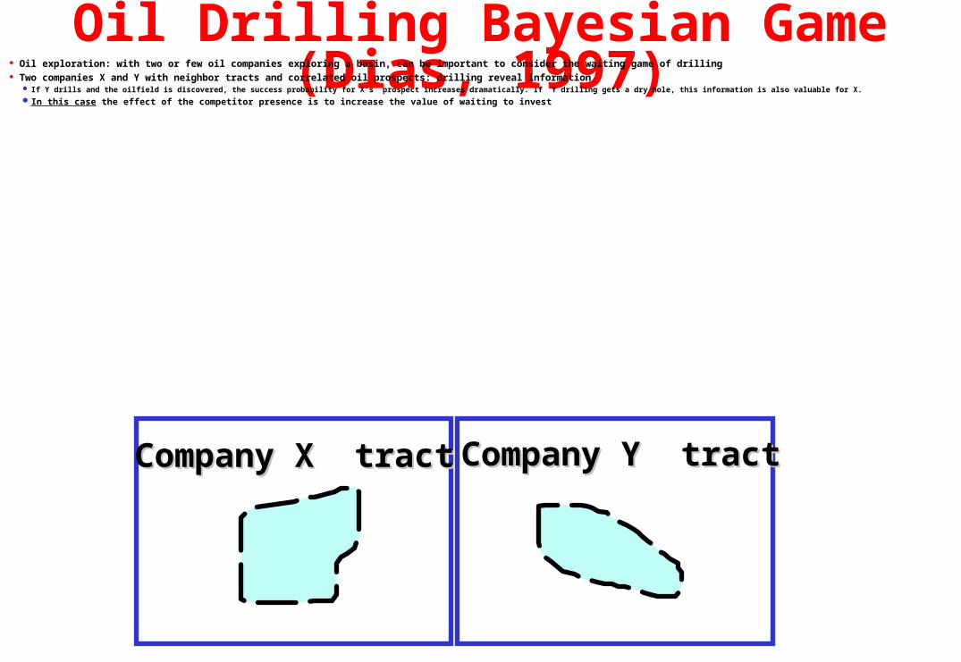
Oil Drilling Bayesian Game (Dias, 1997) Oil exploration: with two or few oil companies exploring a basin, can be important to consider the waiting game of drilling Two companies X and Y with neighbor tracts and correlated oil prospects: drilling reveal information

If Y drills and the oilfield is discovered, the success probability for X’s prospect increases dramatically. If Y drilling gets a dry hole, this information is also valuable for X.

In this case the effect of the competitor presence is to increase the value of waiting to invest

Company X tractCompany X tract Company Y tractCompany Y tract

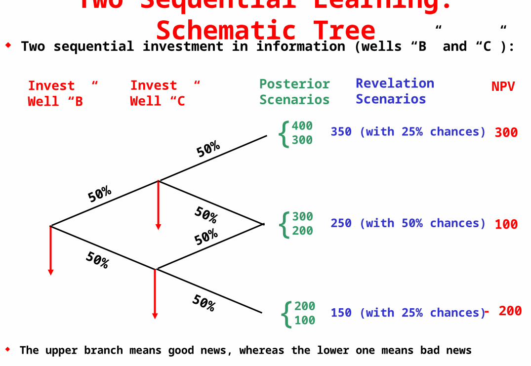
Two Sequential Learning: Schematic Tree Two sequential investment in information (wells “B” and “C”):

InvestWell “B”

RevelationScenarios

PosteriorScenarios

InvestWell “C”

50%

50%

50%

50%

50%

50%

{ 400300

{ 300200

{ 200100

350 (with 25% chances)

The upper branch means good news, whereas the lower one means bad news

250 (with 50% chances)

150 (with 25% chances)

NPV

300

100

- 200

Visual FAQ’s on Real Options: 9 Is possible real options theory to recommend

investment in a negative NPV project?

Answer: yes, mainly sequential options with investment revealing new informations Example: exploratory oil prospect (Dias 1997)

Suppose a “now or never” option to drill a wildcatStatic NPV is negative and traditional theory recommends to give up the

rights on the tractReal options will recommend to start the sequential investment, and

depending of the information revealed, go ahead (exercise more options) or stop

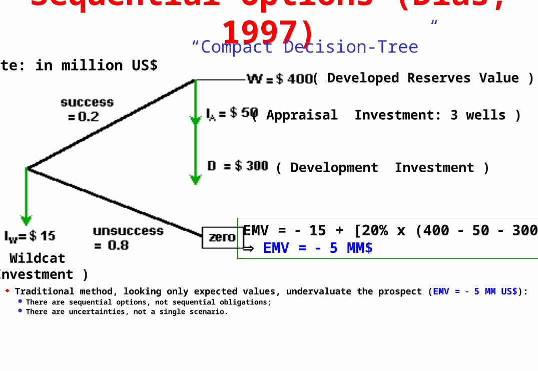
Sequential Options (Dias, 1997)

Traditional method, looking only expected values, undervaluate the prospect (EMV = 5 MM US$): There are sequential options, not sequential obligations; There are uncertainties, not a single scenario.

( Wildcat Investment )

( Developed Reserves Value )

( Appraisal Investment: 3 wells )

( Development Investment )

Note: in million US$“Compact Decision-Tree”

EMV = 15 + [20% x (400 50 300)] EMV = 5 MM$

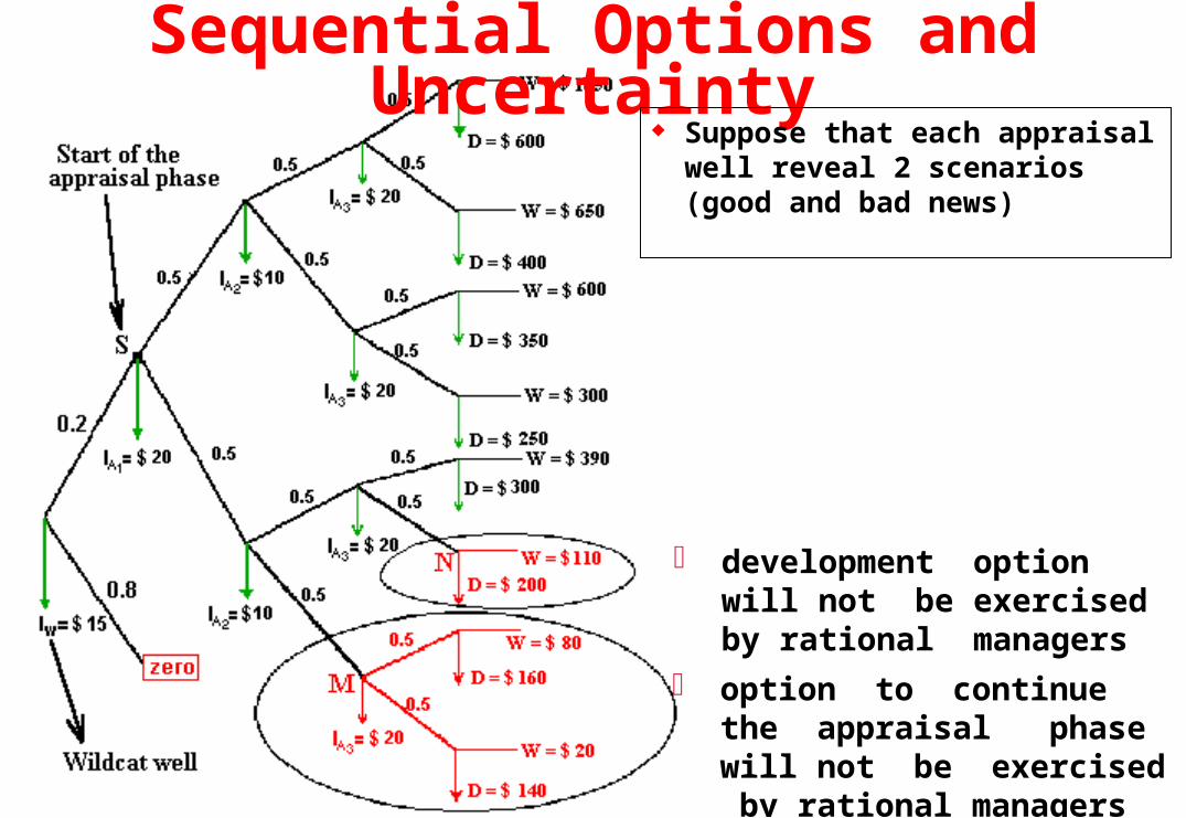
Sequential Options and Uncertainty Suppose that each appraisal

well reveal 2 scenarios (good and bad news)

development option will not be exercised by rational managers

option to continue the appraisal phase will not be exercised by rational managers

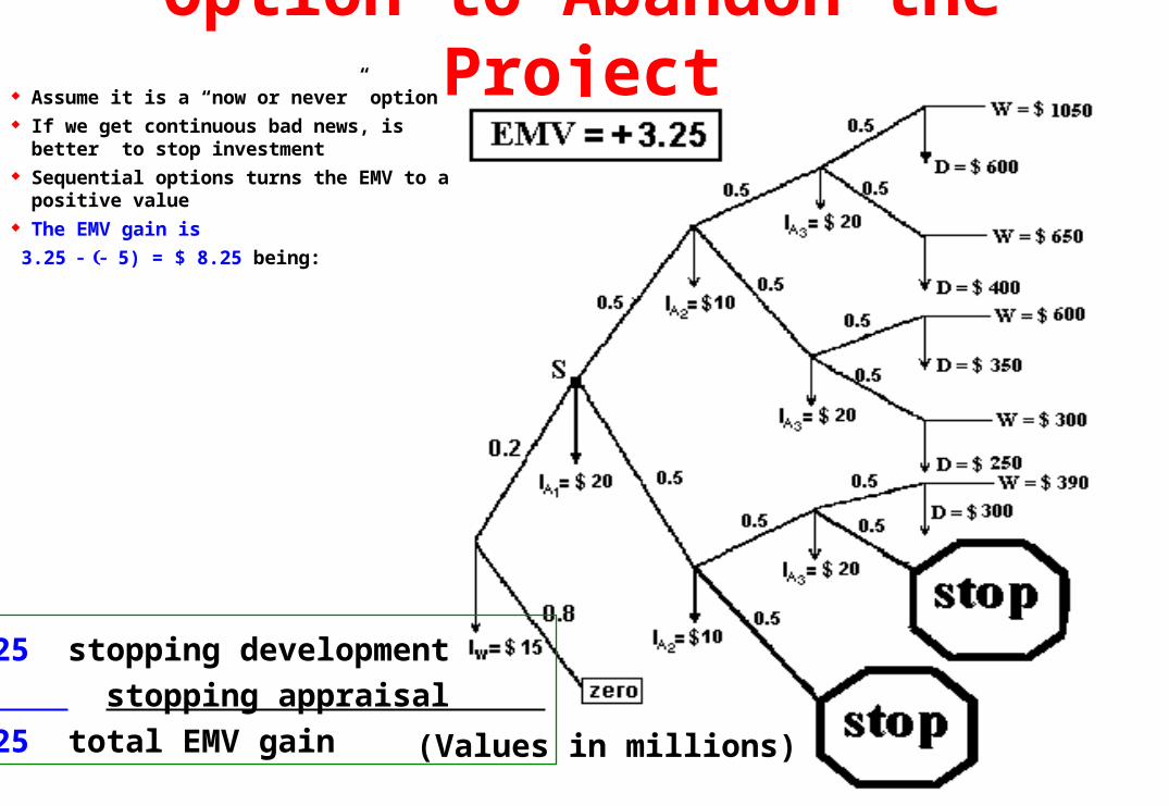
Option to Abandon the Project Assume it is a “now or never” option If we get continuous bad news, is better to stop

investment Sequential options turns the EMV to a positive

value The EMV gain is

3.25 5) = $ 8.25 being:

(Values in millions)

$ 2.25 stopping development

$ 6 stopping appraisal

$ 8.25 total EMV gain

Economic Quality of the Developed Reserve Imagine that you want to buy 100 million barrels of developed oil

reserves. Suppose a long run oil price is 20 US$/bbl. How much you shall pay for the barrel of developed reserve?

One reserve in the same country, water depth, oil quality, OPEX, etc., is more valuable than other if is possible to extract faster (higher productivity index, higher quantity of wells)

A reserve located in a country with lower fiscal charge and lower risk, is more valuable (eg., USA x Angola)

As higher is the percentual value for the reserve barrel in relation to the barrel oil price (on the surface), higher is the economic quality: value of one barrel of reserve = v = q . P Where q = economic quality of the developed reserve The value of the developed reserve is v times the reserve size (B)

Monte Carlo Simulation of Uncertainties Simulation will combine uncertainties (technical and market) for the

equation of option exercise: NPV(t)dyn = q . B . P(t) D(B)

Reserve Size (B) (only at t = trevelation)

(in million of barrels)

Minimum = 300Most Likely = 500Maximum = 700

Oil Price (P) ($/bbl) (from t = 0 until t = T)

Mean = 18 US$/bbl Standard-Deviation:

changes with the time

Parameter Distribution Values (example)

Economic Quality of the Developed Reserve (q) (only at t = trevelation)

Minimum = 10% Most Likely = 15% Maximum = 20%

In the case of oil price (P) is performed a risk-neutral simulation of its stochastic process, because P(t) fluctuates continually along the time

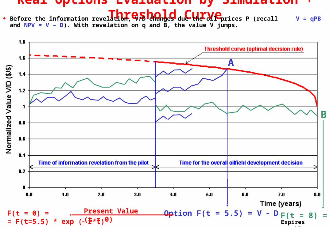
Real Options Evaluation by Simulation + Threshold Curve Before the information revelation, V/D changes due the oil prices P (recall V = qPB and NPV = V – D). With revelation

on q and B, the value V jumps.

A

Option F(t = 5.5) = V DF(t = 0) == F(t=5.5) * exp (r*t)

Present Value (t = 0)

B

F(t = 8) = 0Expires Worthless

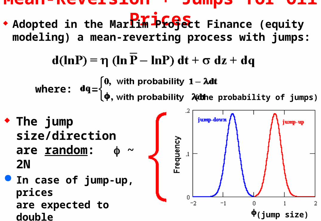
Mean-Reversion + Jumps for Oil Prices Adopted in the Marlim Project Finance (equity

modeling) a mean-reverting process with jumps:

The jump size/direction are random: ~ 2N

In case of jump-up, prices are expected to double OBS: E()up = ln2 = 0.6931

In case of jump-down, prices are expected to halve OBS: ln(½) = ln2 = 0.6931

where:(the probability of jumps)

(jump size)

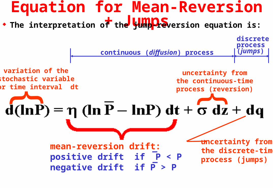
Equation for Mean-Reversion + Jumps The interpretation of the jump-reversion equation is:

mean-reversion drift:positive drift if P < Pnegative drift if P > P

{uncertainty fromthe continuous-timeprocess (reversion){variation of the

stochastic variablefor time interval dt

uncertainty fromthe discrete-timeprocess (jumps)

continuous (diffusion) process

discreteprocess(jumps)

Example in E&P with the Options Lens In a negotiation, important mistakes can be done if we don´t

consider the relevant options Consider two marginal oilfields, with 100 million bbl, both non-

developed and both with NPV = 3 millions in the current market conditions The oilfield A has a time to expiration for the rights of only 6 months, while for

the oilfield B this time is of 3 years Cia X offers US 1 million for the rights of each oilfield. Do you

accept the offer? With the static NPV, these fields have no value and even worse, we

cannot see differences between these two fields It is intuitive that these rights have value due the uncertainty and the option to wait

for better conditions. Today the NPV is negative, but there are probabilities for the NPV become positive in the future

In addition, the field B is more valuable (higher option) than the field A