ofr20211065.pdf - Turbidity–Suspended-Sediment ...

Prepared in cooperation with the New York City Department of Environmental Protection

Turbidity–Suspended-Sediment Concentration Regression Equations for Monitoring Stations in the Upper Esopus Creek Watershed, Ulster County, New York, 2016–19

Open-File Report 2021–1065

U.S. Department of the InteriorU.S. Geological Survey

Cover. Collage of three photographs. Top: The Ashokan Reservoir after a storm, Ulster County, New York; photograph by Wae D. Davis, New York City Department of Environmental Protection. Middle: Collection of cross-section samples from the Esopus Creek below Lost Clove Road at Big Indian, N.Y.; photograph by Donald B. Bonville, U.S. Geological Survey. Bottom: Lacustrine sediment consisting of interbedded layers of clay, silt, and fine sand; photograph by Jason Siemion, U.S. Geological Survey.


By Jason Siemion, Donald B. Bonville, Michael R. McHale, and Michael R. Antidormi

Prepared in cooperation with the New York City Department of Environmental Protection

Open-File Report 2021–1065

U.S. Department of the InteriorU.S. Geological Survey

U.S. Geological Survey, Reston, Virginia: 2021

For more information on the USGS—the Federal source for science about the Earth, its natural and living resources, natural hazards, and the environment—visit https://www.usgs.gov or call 1–888–ASK–USGS.

For an overview of USGS information products, including maps, imagery, and publications, visit https://store.usgs.gov/.

Any use of trade, firm, or product names is for descriptive purposes only and does not imply endorsement by the U.S. Government.

Although this information product, for the most part, is in the public domain, it also may contain copyrighted materials as noted in the text. Permission to reproduce copyrighted items must be secured from the copyright owner.

Suggested citation:Siemion, J., Bonville, D.B., McHale, M.R., and Antidormi, M.R., 2021, Turbidity–suspended-sediment concentration regression equations for monitoring stations in the upper Esopus Creek watershed, Ulster County, New York, 2016–19: U.S. Geological Survey Open-File Report 2021–1065, 27 p., https://doi.org/ 10.3133/ ofr20211065.

Associated data for this publication:Siemion, J., Bonville, D.B., and Antidormi, M.R., 2021, Suspended-sediment concentration and turbidity data for sites in the upper Esopus Creek watershed New York, 2016–19: U.S. Geological Survey data release, https://doi.org/10.5066/P9MV3NZ8.

ISSN 2331-1258 (online)

https://doi.org/10.3133/ofr20211065

https://doi.org/10.5066/P9MV3NZ8

iii

Acknowledgments

This project was funded by the New York City Department of Environmental Protection. The work would not have been possible without the field work of Noel Deyette, of the New York Water Science Center, and Heather A. Dormady and Luis Rodríguez, formerly of the New York Water Science Center. The report benefitted from detailed reviews by Timothy F. Hoffman, Zulimar Lucena, and Paul Diaz.

v

ContentsAcknowledgments ........................................................................................................................................iiiAbstract ...........................................................................................................................................................1Introduction.....................................................................................................................................................1Study Methods ...............................................................................................................................................3

Data Collection ......................................................................................................................................3Data Analysis .........................................................................................................................................3

Development of Cross-Section Coefficients and Regression Equations .............................................4Cross-Section Coefficients .................................................................................................................4Turbidity-SSC Regression Equations ...............................................................................................13

Summary........................................................................................................................................................18References Cited..........................................................................................................................................19Appendix 1. Streamflow Duration Curves ............................................................................................20Appendix 2. Turbidity Duration Curves ..................................................................................................24

Figures

1. Map showing locations of the Ashokan reservoir watershed, Esopus Creek, New York, tributary watersheds, and monitoring sites used in the study ...........................2

2. Graphs showing cross-section coefficients as a function of streamflow for 12 monitoring sites and turbidity for 2 monitoring sites in the upper Esopus Creek watershed ......................................................................................................................................9

3. Graphs showing adjusted suspended-sediment concentration as a function of turbidity for 14 monitoring sites in the upper Esopus Creek watershed in New York .....15

Tables

1. Cross-section and point samples used in the development of cross-section coefficients for monitoring sites in the upper Esopus Creek watershed ............................5

2. Diagnostic statistics for turbidity–suspended-sediment concentration regression equations for 14 monitoring sites in the Esopus Creek watershed, New York ......................................................................................................................................14

vi

Conversion FactorsU.S. customary units to International System of Units

Multiply By To obtain

inch (in.) 25.4 millimeter (mm)mile (mi) 1.609 kilometer (km)foot (ft) 0.3048 meter (m)square mile (mi2) 2.590 square kilometer (km2)ounce, fluid (fl. oz) 29.57 milliliter (mL)gallon (gal) 3.785 liter (L)cubic foot per second (ft3/s) 0.02832 cubic meter per second (m3/s)

DatumVertical coordinate information is referenced to the North American Vertical Datum of 1988 (NAVD 88).

Horizontal coordinate information is referenced to the North American Datum of 1983 (NAD 83).

Supplemental InformationConcentrations of suspended sediment in water are given in milligrams per liter (mg/L).

Turbidity is reported in formazin nephelometric units (FNU).

AbbreviationsBCF bias correction factor

Q streamflow

SAID Surrogate Analysis and Index Developer

SLR simple linear regression

SSC suspended-sediment concentration

SSCa adjusted suspended-sediment concentration

USGS U.S. Geological Survey


By Jason Siemion, Donald B. Bonville, Michael R. McHale, and Michael R. Antidormi

AbstractUpper Esopus Creek is the primary tributary to the

Ashokan Reservoir, part of the New York City water-supply system. Elevated concentrations of suspended sediment and turbidity in the watershed of the creek are of concern for the system.

Water samples were collected through a range of stream-flow and turbidity at 14 monitoring sites in the upper Esopus Creek watershed for analyses of suspended-sediment con-centration (SSC) and measurements of turbidity. Analyses of the samples provided data that were used to develop cross-section coefficients and turbidity-SSC regression equations for the monitoring sites for the period October 2016 through September 2019. The equations can be used to estimate SSC at a 15-minute timestep for the monitored sites. The equations can be validated for future use by the collection and analysis of additional data.

IntroductionEsopus Creek, in the Catskill Mountains of New York

State, is part of New York City’s water-supply system. In 1915, a part of the creek’s watershed was dammed to form the Ashokan Reservoir near Boiceville, New York, thereby splitting the creek into upper (upstream from the reservoir) and lower (downstream from the reservoir) segments. The Ashokan Reservoir watershed is 255 square miles (mi2), one

of two reservoirs in the New York City Catskill Reservoir system, and one of six reservoirs in the West-of-Hudson Catskill-Delaware watershed. The upper Esopus Creek water-shed encompasses approximately 192 mi2 from its source, Winnisook Lake, to the Ashokan Reservoir, N.Y. (fig. 1; U.S. Geological Survey [USGS], 2016).

Elevated suspended-sediment concentrations (SSCs) and turbidity are primary water-quality concerns in New York City’s water-supply system (New York State Department of Health, 2017). In the upper Esopus Creek watershed, the main source of water to the Ashokan Reservoir, the active stream corridor and mass wasting from adjacent hillslopes are assumed to be the primary sources of sediment and turbidity to the stream (New York City Department of Environmental Protection, 2017). In 2016, the New York City Department of Environmental Protection, in cooperation with the USGS, began a comprehensive study of suspended sediment and turbidity in the upper Esopus Creek watershed. The general objectives of the study are outlined in the “Upper Esopus Creek Watershed Turbidity/Suspended Sediment Monitoring Study: Project Design Report” (New York City Department of Environmental Protection, 2017). One objective was to develop turbidity-SSC regression equations for 14 monitoring sites. The other objectives depend on reliable estimates of SSC made by using the resulting regression equations. This report describes the field methods used to collect water samples and continuous monitoring data, development of cross-section cor-rection coefficients, application of those coefficients to point samples, and development of turbidity-SSC regression equa-tions needed to estimate SSC from measured turbidity.

2

Turbidity–Suspended-Sediment Concentration Regression Equations, Upper Esopus Creek W

atershed, New

York, 2016–19

Base from National Geographic/Esri digital dataUniversal Transverse Mercator, Zone 18NNorth American Datum of 1983

UpperEsopus Creek

013623700136219503

013621955

01362200

01362286

0136230002

0136232201362336

01362345

01362357

01362368

01362487

01362497

01362500

01362336

Shandaken Tunnel

AshokanReservoir

0 2 MILES

0 2 KILOMETERS

1

1

74°10'74°20'74°30'

42°10'

42°05'

42°

Shandaken Tunnel

USGS Streamflow-gaging station withidentifier

EXPLANATION

Watershed boundary

NEW YORK Study area

Figure 1. Locations of the Ashokan reservoir watershed, Esopus Creek, New York, tributary watersheds, and monitoring sites used in the study.

Study Methods 3

Study Methods

Data Collection

Water samples were collected for analysis of SSC using standard USGS methods (Edwards and Glysson, 1999). Automated samplers were used to collect discrete point samples during storms at predetermined changes in stream stage. The samplers were programmed to rinse and purge the sample line before each sample was collected. Approximately 800 milliliters (mL) of stream water were pumped into a 1-liter bottle for each sample. Cross-section samples were col-lected using the equal-width depth-integrated method either by wading at the measurement section or by using isokinetic sam-plers from a nearby bridge. For samples collected by wading in the stream, a US DH–81 sampler with a plastic bottle, cap, and nozzle was used. When collecting samples from a bridge, a US D–95 sampler with a plastic bottle, cap, and nozzle was deployed from a B-reel and bridge crane. Sampling for development of cross-section correction coefficients consisted of collection of two sample sets referred to as “A” and “B” sets. The A and B sets each consisted of a cross-section sample paired with point samples pumped by the automated sampler before and after cross-section samples were collected. Cross-section and point samples were analyzed for SSC by methods described in Guy (1969) at either the USGS Ohio-Kentucky-Indiana Water Science Center or the Cascade Volcano Observatory sediment laboratories.

Stream stage was measured at 15-minute intervals, streamflow was measured throughout the range in hydro-logic conditions, and streamflow was calculated at a 15-minute timestep using standard USGS methods (Sauer and Turnipseed, 2010; Turnipseed and Sauer, 2010). Streamflow was not calculated at a 15-minute interval at two monitoring locations: Lower Hollow Tree Brook at State Highway 214 at Lanesville, N.Y. (01362345), and Woodland Creek at Wilmot Way at Woodland, N.Y. (01362286). The daily mean streamflow at these sites was estimated by multiplying the known daily mean streamflow at nearby streamgages by the ratio of the respective drainage areas. The gages on Hollow Tree Brook at Lanesville (01362342) and Woodland Creek above mouth at Phoenicia (0136230002) were used for sites 01362345 and 01362286, respectively.

Turbidity was measured with Forest Technology Systems DTS12 turbidity probes at the same 15-minute interval as stage using methods described in Wagner and others (2006). The DTS12 probes were checked with a calibrated field probe and cleaned during routine site visits at least every 6 weeks. The DTS12 turbidity probes were removed and returned to the manufacturer approximately annually for calibration and fac-tory service checks. Calibration and fouling corrections were completed following methods described in Wagner and others (2006). Erroneous data caused by fouling of the probes, ice cover, or equipment malfunction were deleted from the record.

Point samples collected by automated samplers may not be representative of the overall stream cross-section SSC. Therefore, a cross-section coefficient was applied to adjust the point- sample values to be representative of cross-section conditions before development of turbidity-SSC regression equations and computation of suspended-sediment loads (Porterfield, 1972). Cross-section coefficients were developed for each site by dividing the cross-section SSC by the cor-responding point-sample SSC. The SSC for the A and B cross sections were averaged if streamflow and turbidity conditions were stable during the sample collection; otherwise the values were used individually. The turbidity and streamflow associ-ated with each cross-section sample were averaged over the period of sample collection. Samples were rejected if the SSC of either the cross-section sample or point sample was less than 1 milligram per liter (mg/L). Some samples were rejected because of biased point samples, likely the result of fouling by sediment buildup in the sample line orifice and insufficient rinsing of the line before sample collection.

Data Analysis

Cross-section coefficients were plotted as a function of streamflow for all monitoring sites with the exception of the sites Lower Hollow Tree Brook at State Highway 214 at Lanesville and Woodland Creek at Wilmot Way at Woodland. Cross-section coefficients were plotted as a function of turbid-ity at these two sites because 15-minute streamflow was not available. A simple linear regression (SLR) equation or power function was developed for each relation. The SLR or power function was then applied to the point-sample SSC to yield an adjusted SSC representative of the true cross-section SSC.

The methods used in the development of turbidity-SSC regression equations follow those described in USGS Techniques and Methods, book 3, chapter C4 (Rasmussen and others, 2009), with the exception of eliminating serial correla-tion in the sample data. Serial correlation was investigated visually by plotting residuals (the difference between the mea-sured and predicted values) over time. The presence of serial correlation in a dataset violates assumptions of regression analysis and may cause the standard deviation to be underesti-mated (Helsel and others, 2020). Serial correlation was mini-mized, though not eliminated, by removing from the analysis the data for some samples collected during cross-section measurements and by removing the data for some samples collected during storms. The samples removed were collected within a short period of time, generally within an hour of each other. Data removal was random and iterative to minimize selection bias while keeping at least one sample on the rising limb of the hydrograph, near the peak, and on the falling limb, and to cover the range in sediment transport conditions.

Data were analyzed by regression methods using the Surrogate Analysis and Index Developer (SAID) tool (Domanski and others, 2015) to evaluate the log10 turbidity data as the explanatory variable for estimating log10 SSC. The log10 transformation was chosen on the basis of previous work

4 Turbidity–Suspended-Sediment Concentration Regression Equations, Upper Esopus Creek Watershed, New York, 2016–19

in the watershed (Siemion and others, 2016). The distribution of residuals was examined for normality, and plots of residuals as a function of predicted SSC were examined for homosce-dasticity. Cook’s D and the difference in fits (DFFITs) were used to identify sample pairs with high influence or leverage (Helsel and others, 2020). Each sample pair flagged as having high influence or leverage was investigated and removed from the dataset if appropriate. Flagged samples generally had high SSC relative to the paired turbidity. Fouling of the sample line was a possible reason for high SSC relative to paired turbid-ity, especially during conditions of low sediment transport. Retransformation of the log-transformed model introduced a bias in the calculated SSC (Helsel and others, 2020). This bias was corrected using Duan’s Bias Correction Factor (BCF) (Duan, 1983). Regression statistics and metrics, including the root mean square error, coefficient of determination, linear correlation coefficient, model square percent error, the BCF, and the retransformed model (accounting for BCF), for each monitoring site are presented in the following section of this report.

All data used in the development of cross-section coefficients and regression equations are available from the USGS National Water Information System (U.S. Geological Survey, 2020). Sample data and diagnostic plots are available as a USGS data release in Siemion and others (2021).

Development of Cross-Section Coefficients and Regression Equations

Cross-section coefficients were developed for each of 14 monitoring sites in the upper Esopus Creek watershed, and regression equations were developed to compute 15-minute SSC from October 1, 2016, to September 30, 2019, for each monitoring site. Streamflow and turbidity duration curves showing conditions when samples were collected and the range in streamflow and turbidity are presented in appen-dixes 1 and 2, respectively.

Cross-Section Coefficients

The cross-section coefficients for the 14 monitoring sites were developed using 3 years of data and include data from 5 to 10 samples from each site. The coefficients developed on the basis of these relatively small datasets for some sites resulted in one or two high-leverage samples and will need to be revisited when additional validation samples become available. Application of the coefficients in the development of regression equations resulted in adjustments to SSC ranging from −46 percent during conditions of low sediment transport to 26 percent during conditions of high sediment transport. Large coefficients during conditions of low sediment transport did not result in large magnitude changes to the low SSC mea-sured during those conditions. Relatively large adjustments to SSC during conditions of high sediment transport resulted in

substantial changes to already high SSC. However, 10 of the 13 cross-section coefficients resulted in adjustments of 11 per-cent or less during conditions of high sediment transport. The flashy nature of streamflow at the monitoring sites presented challenges in collecting cross-section samples through the full range in streamflow and sediment transport conditions. Nonetheless, extrapolation of the coefficients beyond the range of sampled conditions was limited to 1 percent or less of the streamflows measured during the study period at all but one monitoring location.

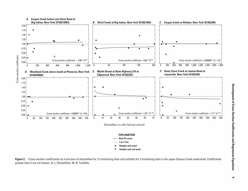
At monitoring site Esopus Creek below Lost Clove Road at Big Indian, N.Y. (0136219503), the sampler intake was mounted on a bridge abutment on the right bank, near the thal-weg of the channel in a well-mixed part of the stream. Data from eight sample sets were used to develop the cross-section coefficient (appendix figs. 1.1 and 2.1; table 1). A power function of cross-section coefficient = 0.86 * Q0.03, where Q is streamflow, was developed (fig. 2A). This resulted in a 12-percent adjustment of SSC in the point samples at 2 cubic feet per second (ft3/s) and a 6-percent adjustment at 1,100 ft3/s, the minimum and maximum streamflows at which cross-section samples were collected. Extrapolation of the power function beyond 1,100 ft3/s resulted in an adjustment in SSC of 9 percent at the maximum streamflow of 2,600 ft3/s during the study period. The derived coefficients beyond 1,100 ft3/s cover 0.2 percent of the observed streamflows during the study period.

At monitoring site Birch Creek at Big Indian, N.Y. (013621955), the sampler intake was mounted relatively low in the water column in the center of the channel. Data from 10 sample sets were used to develop the cross-section coeffi-cient for this site (figs. 1.1 and 2.1; table 1). A power func-tion of cross-section coefficient = 0.6 * Q0.06 was developed (fig. 2B). This resulted in a −37-percent adjustment to SSC in the point samples at 2 ft3/s and a −17-percent adjustment at 203 ft3/s, the minimum and maximum streamflows at which cross-section samples were collected. Extrapolation of the power function to flows greater than 203 ft3/s resulted in an adjustment of −11 percent at 725 ft3/s, the maximum stream-flow during the study period. The derived coefficients beyond 203 ft3/s cover 1 percent of the observed streamflows during the study period.

At monitoring site Esopus Creek at Allaben, N.Y. (01362200), the sampler intake was mounted on a bridge abutment on the right bank, near the thalweg of the channel in a well-mixed part of the stream. Data from seven sample sets were used to develop the cross-section coefficient (figs. 1.1 and 2.1; table 1). A SLR of cross-section coefficient = 0.000004 * Q + 1.03 was developed (fig. 2C). This resulted in a 3-percent adjustment of SSC in the point samples at stream-flows of 7 ft3/s and a 4-percent adjustment at 1,700 ft3/s, the minimum and maximum streamflows at which cross-section samples were collected. Extrapolation of the SLR beyond 1,700 ft3/s resulted in an adjustment in SSC of 4 percent at the

Development of Cross-Section Coefficients and Regression Equations 5

Table 1. Cross-section and point samples used in the development of cross-section coefficients for monitoring sites in the upper Esopus Creek watershed.

[Turbidity in formazin nephelometric units. Streamflow in cubic feet per second. SSC, suspended-sediment concentration in milligrams per liter; NA, not avail-able; <, less than]

Sample start date and timeCross-

section(s)

Cross-section

SSC

Point SSC

Cross-section coefficients

Turbidity StreamflowIncluded in

cross-section coefficient?

Esopus Creek below Lost Clove Road at Big Indian, New York (0136219503)

2/25/2017 13:30 A 28 24 1.17 NA 519 Yes8/24/2017 08:45 A, B <1 <1 NA 1.30 32.2 No1

1/23/2018 12:40 A 147 458 0.32 210 542 No2

1/23/2018 13:10 B 123 108 1.14 167 539 Yes4/4/2018 10:30 A, B 2 3.5 0.57 3.20 118 Yes4/4/2018 13:05 A 6 8 0.75 5.27 139 Yes7/23/2018 12:40 A 61 23 2.65 19.7 121 No3

7/23/2018 13:05 B 30 17 1.76 17.6 119 Yes4/15/2019 09:00 A, B 143 154 0.93 89.4 1,100 Yes8/7/2019 14:02 A <1 2 NA 0.3 9.56 No2

8/7/2019 14:10 B 1 1 1.0 0.5 9.76 Yes11/1/2019 12:02 A, B 78 65 1.2 52.3 1,020 Yes

Birch Creek at Big Indian, New York (013621955)

2/25/2017 14:45 A, B 26.5 35 0.76 23.5 152 Yes8/24/2017 08:10 A, B 3 4 0.75 4.60 8.49 Yes1/23/2018 11:20 A 104 233 0.45 110 206 No2

4/4/2018 12:00 A, B 22.5 28.5 0.79 26.0 116 Yes4/16/2018 09:45 A 153 105 1.46 152 153 No3

4/16/2018 10:15 B 170 223 0.76 200 183 Yes7/17/2018 10:25 A, B 17 14 1.21 8.0 6.71 Yes12/21/2018 10:20 A, B 78.5 77.5 1.01 134 203 Yes4/17/2019 12:00 A 42 42 1.0 135 135 Yes6/4/2019 11:50 A, B 1 3.5 0.29 9.1 18.8 Yes8/7/2019 13:45 A, B 3 3.66 0.82 6.9 4.99 Yes10/7/2019 12:30 A, B 1 2 0.5 3.5 4.46 Yes

Esopus Creek at Allaben, New York (01362200)

3/27/2017 11:05 A 5 11 0.45 7.75 160 No2

3/27/2017 11:20 B 6 6 1.0 7.75 161 Yes8/24/2017 10:05 A, B 4.5 4 1.13 3.2 53.9 Yes10/30/2017 07:45 A 232 229 1.01 213 1,370 Yes10/30/2017 08:40 B 204 NA NA 188 1,280 No4

4/4/2018 09:10 A, B 3.5 4 0.88 4.28 401 Yes7/25/2018 12:25 A, B 13 11.5 1.13 13.7 481 Yes4/15/2019 10:30 A 215 204 1.05 111 1,700 Yes7/17/2019 12:35 A, B 2 2 1.0 2.6 28.7 Yes

Woodland Creek at Wilmot Way near Woodland, New York (01362286)

3/27/2017 12:00 A 9 6 1.5 12.8 NA Yes8/24/2017 11:00 A, B 1 3.5 0.29 0.6 NA Yes10/24/2017 12:28 A, B 3 4 0.75 4.90 NA Yes


Table 1. Cross-section and point samples used in the development of cross-section coefficients for monitoring sites in the upper Esopus Creek watershed.—Continued



section(s)

Cross-section

SSC

Point SSC




Woodland Creek at Wilmot Way near Woodland, New York (01362286)—Continued

10/29/2017 17:10 A, B 23 27 0.85 37.8 NA Yes11/6/2017 16:35 A, B 42 468 0.09 103 NA No2

3/20/2018 18:00 A, B 7.5 604 0.01 19.4 NA No2

3/28/2018 09:34 A, B 10.5 12.5 0.84 15.4 NA Yes7/17/2019 11:45 A, B 2.5 2.0 1.25 1.25 NA Yes10/7/2019 10:55 A 2 1.5 1.33 2.0 NA Yes10/7/2019 11:04 B 9 1 9.0 2.0 NA No3

Woodland Creek above mouth at Phonecia, New York (0136230002)

2/25/2017 11:15 A, B 20 22 0.91 25.8 350 Yes10/24/2017 13:25 A, B 40.5 55.5 0.73 80 38 Yes10/29/2017 18:25 A 217 215 1.01 191 319 Yes10/29/2017 19:00 B 274 283 0.97 212 420 Yes7/17/2018 09:20 A, B 5 5 1.0 7.3 6.8 Yes7/17/2019 10:45 A, B 3 3 1.0 3.65 19.4 Yes10/7/2019 12:00 A 1 1 1.0 1.6 7.49 Yes10/7/2019 12:10 B <1 1 NA 1.6 7.68 No1

Myrtle Brook at State Highway 214 at Edgewood, New York (01362322)

2/25/2017 12:56 A, B 12.5 35 0.36 11.1 29.3 No2

4/4/2018 11:43 A, B 1.5 1 1.5 1.15 10.5 Yes7/23/2018 09:25 A, B 26.5 24 1.1 20 24.3 Yes12/21/2018 09:35 A, B 69 74 0.93 54.6 61.3 Yes7/11/2019 11:50 A, B 1 1 1.0 1.9 0.94 Yes10/7/2019 16:25 A, B 1.5 1 1.5 2 0.61 Yes11/1/2019 9:05 A, B 23.5 27 0.87 15.9 58.1 Yes

Stony Clove at Jansen Road at Lanesville, New York (01362336)

2/25/2017 10:45 A, B 28.5 139 0.21 NA 116 No2

8/23/2017 11:40 A, B <1 1 NA 0.5 11 No1

10/29/2017 16:39 A 65 59 1.1 35.7 76.3 Yes10/30/2017 08:05 A, B 190 312 0.61 141 444 Yes6/28/2018 10:40 A, B 2 3 0.67 2 8.09 Yes6/20/2019 11:55 A, B 1.5 1 1.5 2.2 13.1 Yes10/7/2019 15:29 A, B <1 <1 NA 3.2 3.41 No1

11/1/2019 10:03 A, B 76.5 69 1.11 63.5 214 YesHollow Tree Brook at State Highway 214 at Lanesville, New York (01362345)

2/25/2017 13:52 A, B 8.5 15 0.57 6.55 NA Yes8/23/2017 12:40 A, B <1 3 NA 1.8 NA No1

10/29/2017 17:05 A, B 125 116.5 1.07 78.6 NA Yes6/28/2018 10:49 A, B 4.5 5.5 0.82 6.3 NA Yes12/21/2018 10:00 A, B 45.5 46 0.99 37.2 NA Yes





section(s)

Cross-section

SSC

Point SSC




Hollow Tree Brook at State Highway 214 at Lanesville, New York (01362345)—Continued

6/20/2019 12:14 A, B 1.5 2 0.75 2.35 NA Yes10/7/2019 15:55 A, B 2.5 4.33 0.58 6.5 NA Yes

Warner Creek near Chichester, New York (01362357)

3/27/2017 10:15 A, B 8 8 1.0 24.3 21.8 Yes4/4/2017 12:40 A, B 59.5 70 0.85 84.7 206 Yes8/23/2017 10:20 A, B 1 3 0.33 5.87 8.38 No2

10/29/2017 16:00 A 97 91 1.07 79.2 41 Yes10/29/2017 16:15 B 107 123 0.87 104 58.5 Yes6/28/2018 09:20 A 6 11 0.55 12.2 13.4 No2

6/28/2018 09:30 B 6 7 0.86 13.0 13.1 Yes7/23/2018 10:25 A 83 64 1.3 66.6 200 No3

7/23/2018 10:45 B 60 54 1.11 60.4 194 Yes11/6/2018 12:40 A, B 42 41.5 1.01 118 76.1 Yes3/15/2019 12:50 A 37 79 0.47 137 23.5 No2

3/15/2019 13:10 B 38 37 1.03 119 24.7 Yes7/11/2019 12:35 A, B 2 2 1.0 6.80 5.58 Yes10/7/2019 15:04 A, B <1 1 NA 1.95 3.69 No1

Ox Clove near mouth at Chichester, New York (01362368)

3/27/2017 09:37 A, B 20.5 24 0.85 37.5 10.4 Yes8/23/2017 09:15 A, B 3.5 6 0.58 5.9 2 Yes10/29/2017 15:40 A 116 182 0.64 166 4.68 No4

10/29/2017 15:45 B 136 182 0.75 166 4.68 Yes6/28/2018 09:50 A 41 10 4.10 10.3 2.57 No3

6/28/2018 10:00 B 13 10 1.30 10.1 2.53 Yes7/23/2018 13:00 A, B 28 30.5 0.92 26.5 18.9 Yes12/21/2018 10:25 A 78 107 0.73 158 147 Yes12/21/2018 10:45 B 77 71 1.08 162 144 Yes6/20/2019 11:05 A, B 2.5 3.66 0.68 8.1 5.37 Yes10/7/2019 14:16 A, B 1.5 2.5 0.6 5.2 1.77 Yes

Stony Clove Creek below Ox Clove at Chichester, New York (01362370)

2/25/2017 15:08 A, B 32.5 43.5 0.75 32.6 362 Yes4/4/2018 09:40 A, B 65.5 68 0.96 67.2 497 Yes8/23/2017 08:25 A, B 4 4 1.0 2.0 35.8 Yes10/29/2017 18:48 A 1,250 1,036 1.21 707 1,220 Yes6/28/2018 10:10 A 117 11 10.64 18.0 42.8 No3

6/28/2018 10:10 B 10 11 0.91 16.0 42.8 Yes12/21/2018 12:00 A, B 298 199 1.5 152 1,098 Yes6/20/2019 10:35 A, B 2.5 4 0.63 4.90 55.3 Yes11/1/2019 11:55 A, B 49 44.6 1.10 59.2 585 Yes





section(s)

Cross-section

SSC

Point SSC




Beaver Kill at Mount Tremper, New York (01362487)

3/27/2017 09:20 A, B 39 43.5 0.9 70.2 113 Yes8/24/2017 12:15 A, B <1 48 NA 2.07 5.16 No1,2

4/4/2018 09:40 A, B 3.5 4.5 0.78 2.15 74.8 Yes6/28/2018 08:39 A, B 117 115 1.02 62.0 108 Yes7/25/2018 09:55 A, B 171 177 0.97 73.1 967 Yes3/15/2019 13:42 A, B 150 135 1.11 190 151 Yes7/11/2019 13:40 A, B 1 1.5 0.67 0.85 8.82 Yes10/7/2019 14:45 A, B 2 1.7 1.18 2.1 5.27 Yes

Little Beaver Kill at Beechford near Mount Tremper, New York (01362497)

3/27/2017 10:10 A, B 9 11.5 0.78 10.4 88.1 Yes8/24/2017 13:15 A, B 9 34 0.26 1.4 1.22 No2

4/4/2018 08:35 A, B 1.5 2 0.75 1.4 34.8 Yes6/28/2018 08:14 A, B 13 13 1.0 12.2 24.6 Yes8/7/2019 12:33 A, B 2 1.7 1.18 1.7 10.5 Yes10/7/2019 15:10 A, B 1 25 0.04 0.6 3.95 No2

Esopus Creek at Coldbrook, New York (01362500)

4/6/2017 12:15 A 15 76 0.2 11.2 2,120 No2

4/6/2017 13:49 B 16 17 0.94 13.7 2,180 Yes10/24/2017 14:50 A, B 54.5 45.5 1.2 61.9 582 Yes10/30/2017 11:10 A 166 NA NA 167 4,210 No4

10/30/2017 12:00 B 149 113 1.32 153 3,950 Yes7/17/2018 11:30 A 7 13 0.54 5.75 268 No2

7/17/2018 11:45 B 6 5 1.2 5.65 270 Yes12/21/2018 12:20 A, B 356 200 1.78 154 6,990 No3

8/7/2019 11:35 A, B 5.5 5.67 0.97 9 317 Yes10/17/2019 8:40 A 38 35.5 1.07 24.4 1,250 Yes10/17/2019 9:49 B 33 27.5 1.2 20.4 1,134 Yes

1Sample not included in cross-section coefficient because the SSC was <1 milligram per liter.2Sample not included in cross-section coefficient because autosampler line was fouled.3Sample not included in cross-section coefficient because of suspected problem with cross-section sample.4Sample not included in cross-section coefficient because corresponding point or cross-section sample not collected.


9

Cros

s-se

ctio

n co

effic

ient

Streamflow, in cubic feet per second

EXPLANATIONBest fit curve1 to 1 lineSample sets usedSample sets not used

2.00

1.75

1.50

1.25

1.00

0.75

0.50

0.25

0.00

2.00

1.75

1.50

1.25

1.00

0.75

0.50

0.25

0.00

0 200 400 600 800 1,000 1,200

0 50 100 150 200 250 300 350 400 450

0 50 100 150 200

0 10 20 30 40 50 60 70

0 200 400 600 800 1,000 1,200 1,400 1,600 1,800

0 50 100 150 200 250 300 350 400 450

Cross-section coefficient = 0.86 * Q 0.03

A. Esopus Creek below Lost Clove Road at Big Indian, New York (0136219503) B. Birch Creek at Big Indian, New York (013621955)

Cross-section coefficient = 0.60 * Q 0.06

C. Esopus Creek at Allaben, New York (01362200)

Cross-section coefficient = 0.000004 * Q + 1.03

D. Woodland Creek above mouth at Phonecia, New York (0136230002)

Cross-section coefficient = 0.00005 * Q + 0.94

E. Myrtle Brook at State Highway 214 at Edgewood, New York (01362322)

Cross-section coefficient = 1.30 * Q −0.06

F. Stony Clove Creek at Jansen Road at Lanesville, New York (01362336)

Cross-section coefficient = 1.17 * Q −0.05

Figure 2. Cross-section coefficients as a function of streamflow for 12 monitoring sites and turbidity for 2 monitoring sites in the upper Esopus Creek watershed. Coefficients greater than 2 are not shown. A–L, Streamflow. M, N, Turbidity.

10


atershed, New

York, 2016–19

0 200 400 600 800 1,000 1,2000 50 100 1502500 50 100 150 200

0 20 40 60 800 200 400 600 800 1,000

1,400

0 500 1,000 1,500 2,000 2,500 3,000 3,500 4,000 4,500

25 75 125

100

Cros

s-se

ctio

n co

effic

ient

Streamflow, in cubic feet per second


2.00

1.75

1.50

1.25

1.00

0.75

0.50

0.25

0.00

2.00

1.75

1.50

1.25

1.00

0.75

0.50

0.25

0.00

G. Warner Creek near Chichester, New York (01362357)

Cross-section coefficient = 0.000004 Q + 0.98

J. Beaver Kill at Mount Tremper, New York (01362487)

Cross-section coefficient = 0.86 Q 0.02

H. Ox Clove near mouth at Chichester, New York (01362368)


K. Little Beaver Kill at Beechford, New York (01362497)

I. Stony Clove Creek below Ox Clove at Chichester, New York (01362370)


L. Esopus Creek at Coldbrook, New York (01362500)


Figure 2.—Continued


11

Cros

s-se

ctio

n co

effic

ient


Turbidity, in formazin nephelometric units

2.00

1.75

1.50

1.25

1.00

0.75

0.50

0.25

0.000 20 40 60 80 100 120 0 20 40 60 80 100

M. Woodland Creek at Wilmot Way near Woodland, New York (01362286)

Cross-section coefficient = – 0.0004 turbidity + 0.98

N. Hollow Tree Brook at State Highway 214 at Lanesville, New York (01362345)

Cross-section coefficient = 0.54 turbidity0.15



maximum streamflow of 3,090 ft3/s during the study period. The derived coefficients beyond 1,700 ft3/s cover 0.2 percent of the observed streamflows during the study period.

At monitoring site Woodland Creek above mouth at Phoenicia, N.Y. (0136230002), the sampler intake was mounted on a bridge abutment on the left bank, near the thal-weg of the channel in a well-mixed part of the stream. Data from six sample sets were used to develop the cross-section coefficient (table 1, figs. 1.1 and 2.1). A SLR of cross-section coefficient = 0.00005 * Q + 0.94 was developed (fig. 2D). This resulted in a −6-percent adjustment of SSC in the point samples at streamflows of 3 ft3/s and a −4-percent adjust-ment at 420 ft3/s, the minimum and maximum streamflows at which cross-section samples were collected. Extrapolation of the SLR beyond 420 ft3/s resulted in an adjustment in SSC of 7 percent at the maximum streamflow of 2,640 ft3/s during the study period. The derived coefficients beyond 420 ft3/s cover 1 percent of the observed streamflows during the study period.

At monitoring site Myrtle Brook at State Highway 214 at Edgewood, N.Y. (01362322), the sampler intake was mounted on top of a boulder set in the streambed near the thalweg of the channel. The stream falls 3–4 feet (ft) from a box culvert into the channel 20 ft upstream from the sample line intake creating a well-mixed environment. Data from six sample sets were used to develop the cross-section coefficient (figs. 1.1 and 2.1; table 1). A power function of cross-section coef-ficient = 1.3 * Q−0.06 was developed (fig. 2E). This resulted in a 29-percent adjustment of SSC in the point samples at 0.25 ft3/s and a 1-percent adjustment at 61 ft3/s, the minimum and maximum streamflows at which cross-section samples were collected. Extrapolation of the power function beyond 61 ft3/s resulted in an adjustment in SSC of −3 percent at the maximum streamflow of 123 ft3/s during the study period. The derived coefficients beyond 61 ft3/s cover 0.2 percent of the observed streamflows during the study period.

At monitoring site Stony Clove at Jansen Road at Lanesville, N.Y. (01362336), the sampler intake was mounted on a bridge abutment on the right bank relatively low in the water column near the thalweg of the channel. Data from five sample sets were used to develop the cross-section coeffi-cient (table 1, figs. 1.1 and 2.1). A power function of cross-section coefficient = 1.17 * Q−0.05 was developed (fig. 2F). This resulted in a 17-percent adjustment of SSC in the point samples at 1 ft3/s and a −14-percent adjustment at 444 ft3/s, the minimum and maximum streamflows at which cross-section samples were collected. Extrapolation of the power function beyond 444 ft3/s resulted in an adjustment in SSC of −18 per-cent at the maximum streamflow of 1,320 ft3/s during the study period. The derived coefficients beyond 444 ft3/s cover 1 percent of the observed streamflows during the study period. Sand size particles mobilized from the stream bed during high streamflows at this site may be captured by the sampler intake, thereby biasing the point-sample SSC high in comparison to the cross-section samples. This conclusion is supported by comparison of the percentage of suspended sediment less than 0.125 millimeter (mm) in size in cross-section sample sets.

Samples collected by the automated sampler during cross-section sampling generally contained a greater percentage of larger particles than the associated cross-section samples.

At monitoring site Warner Creek near Chichester, N.Y. (01362357), the sampler intake was mounted on the down-stream side of a constructed rock vane near the thalweg of the channel. The stream flows through a series of cobble riffles for 200 ft upstream from the rock vane, creating a well-mixed environment. Data from nine sample sets were used to develop the cross-section coefficient (table 1, figs. 1.1 and 2.1). A SLR of cross-section coefficient = 0.000004 * Q + 0.98 was developed (fig. 2G). This resulted in a −2-percent adjustment of SSC in the point samples through the range of streamflows at which cross-section samples were collected, from 2 to 206 ft3/s, and at the maximum streamflow of 855 ft3/s during the study period. The derived coefficients beyond 206 ft3/s cover 1 percent of the observed streamflows during the study period.

At monitoring site Ox Clove near mouth at Chichester, N.Y. (01362368), the sampler intake was mounted at the head of a small pool near the thalweg of the channel. The stream flows through a series of boulder riffles for 100 ft upstream from the sampler intake, creating a well-mixed environment. Data from nine sample sets were used to develop the cross-section coefficient (table 1, figs. 1.1 and 2.1). A power function of cross-section coefficient = 0.72 * Q0.05 was developed (fig. 2H). This resulted in a −28-percent adjustment of SSC in the point samples at 1 ft3/s and a −8-percent adjustment at 145 ft3/s, the minimum and maximum streamflows at which cross-section samples were collected. Extrapolation of the power function beyond 145 ft3/s resulted in an adjustment in SSC of −3 percent at the maximum streamflow of 426 ft3/s during the study period. The derived coefficients beyond 145 ft3/s cover 1 percent of the observed streamflows during the study period.

At monitoring site Stony Clove below Ox Clove at Chichester, N.Y. (01362370), the sampler intake was mounted on a boulder on the left bank in an area that may not mix completely during high streamflows. Data from eight sample sets were used to develop the cross-section coefficient (table 1, figs. 1.1 and 2.1). A power function of cross-section coeffi-cient = 0.52 * Q0.11 was developed (fig. 2I). This resulted in a −41-percent adjustment of SSC in the point samples at 3 ft3/s and a 14-percent adjustement at 1,220 ft3/s, the minimum and maximum streamflows at which cross-section samples were collected. Extrapolation of the power function beyond 1,220 ft3/s resulted in an adjustment in SSC of 26 percent at the maximum streamflow of 3,210 ft3/s during the study period. The derived coefficients beyond 1,220 ft3/s cover 1 percent of the observed streamflows during the study period. The cross-section coefficient is supported by comparison of the percentage of suspended sediment less than 0.125 mm in size in cross-section sampling sets. Samples collected by the automated sampler generally contained a greater percentage of finer particles than the associated cross-section samples, thus biasing the point samples low in SSC as compared to corre-sponding cross-section samples.


At monitoring site Beaver Kill at Mount Tremper, N.Y. (01362487), the sampler intake was mounted on a bridge abut-ment on the right bank. The stream flows through a series of riffles for 100s of feet upstream from the sampler intake, creat-ing a well-mixed environment. The pool in which the intake is mounted maintains a good connection to the stream during storms. Data from seven sample sets were used to develop the cross-section coefficient (table 1, figs. 1.1 and 2.1). A power function of cross-section coefficient = 0.86 * Q0.02 was developed (fig. 2J). This resulted in a −14-percent adjustment of SSC in the point samples at 1 ft3/s and a −1-percent adjust-ment at 967 ft3/s, the minimum and maximum streamflows at which cross-section samples were collected. Extrapolation of the power function beyond 967 ft3/s resulted in an adjust-ment in SSC of 1 percent at the maximum streamflow of 2,960 ft3/s during the study period. The derived coefficients beyond 967 ft3/s cover 0.4 percent of the observed stream-flows during the study period. One cross-section sample event collected during high sediment transport conditions had high leverage on the power function; however, this resulted in only a 1-percent adjustment to point-sample SSC at the maximum streamflow during the study period.

A small dataset prevented the development of a cross-section coefficient for the Little Beaver Kill at Beechford, N.Y. (01362497). Only four cross-section sample sets were collected at that site, at flows ranging from 1 to 88.1 ft3/s. The few data available would have resulted in large adjustments to the point SSC and required extrapolation for 10 percent of the streamflows during the study period. Concentrations and loads derived for this site should only be considered representative of conditions at the point sampler intake.

At monitoring site Esopus Creek at Coldbrook, N.Y. (01362500), the sampler intake was mounted 35 ft from the left bank on a boulder. The channel is 250 ft wide at the sam-pler intake position, with the thalweg towards the center of the channel. Data from seven sample sets were used to develop the cross-section coefficient (table 1, figs. 1.1 and 2.1). A power function of cross-section coefficient = 0.97 * Q0.02 was developed (fig. 2L). This resulted in a 2-percent adjustment of SSC in the point samples at 10 ft3/s and a 14-percent adjust-ment at 3,990 ft3/s, the minimum and maximum streamflows at which cross-section samples were collected. Extrapolation of the power function beyond 3,990 ft3/s resulted in an adjust-ment in SSC of 17 percent at the maximum streamflow of 13,600 ft3/s during the study period. The derived coefficients beyond 3,990 ft3/s cover 0.9 percent of the observed stream-flows during the study period.

At monitoring site Woodland Creek at Wilmot Way at Woodland, N.Y. (01362286), the sampler intake was mounted on a boulder towards the right bank of the 20-ft-wide channel. The stream flows through a series of riffles for 100 ft upstream from the sampler intake, thereby creating a well-mixed envi-ronment. Data from seven sample sets were used to develop the cross-section coefficient (table 1, figs. 1.1 and 2.1). A SLR of cross-section coefficient = −0.0004 * turbidity + 0.98 was developed (fig. 2M). This resulted in a −2-percent adjustment

of SSC in the point samples at a turbidity of 1 formazin neph-elometric unit (FNU) and a −4-percent adjustment at 38 FNU, the minimum and maximum turbidity at which cross-section samples were collected. The cross-section coefficient was held constant at −4 percent beyond 38 FNU. The derived coeffi-cients beyond 38 FNU cover 8 percent of the observed turbid-ity values during the study period.

At monitoring site Hollow Tree Brook at State Highway 214 at Lanesville, N.Y. (01362345), the sampler intake was mounted on a boulder towards the right bank near the thalweg of the 25-ft-wide channel. The stream flows through a series of riffles for 75 ft upstream from the sample line intake, thereby creating a well-mixed environment. Six sample sets were used to develop the cross-section coefficient (table 1, figs. 1.1 and 2.1). A power function of cross-section coefficient = 0.54 * turbidity0.15 was developed (fig. 2N). This resulted in a −46-percent adjustment of SSC in the point samples at a turbidity of 1 FNU and a 4-percent adjustment at 78 FNU, the minimum and maximum turbidity at which cross-section samples were collected. The cross-section coefficient was held constant at 4 percent beyond 78 FNU. The derived coefficients beyond 78 FNU cover 0.1 percent of the observed turbidity values during the study period.

Turbidity-SSC Regression Equations

The turbidity-SSC regression equation (table 2, fig. 3A) for Esopus Creek below Lost Clove Road at Big Indian, N.Y. (0136219503), was based on 53 of 93 concurrent values of adjusted SSC (SSCa) and turbidity made at the site from December 18, 2016, to September 3, 2019. Samples were col-lected throughout most of the range of continuously observed streamflow and turbidity (figs. 1.1 and 2.1). Thirty-three observations were removed from the dataset to minimize serial correlation. Seven observations that were determined to have high influence also were removed from the dataset.

The turbidity-SSC regression equation (table 2, fig. 3B) for Birch Creek at Big Indian, N.Y. (013621955), was based on 67 of 113 concurrent values of SSCa and turbidity made at the site from December 1, 2016, to August 21, 2019. Samples were collected through most of the range of continuously observed streamflow and turbidity (figs. 1.1 and 2.1). Six observations were determined to have high influence and were removed from the dataset, and 40 additional observations were removed from the dataset to minimize serial correlation. The residual versus time plot for this regression equation suggested serial correlation was still present after removal of the 40 observations; the sign of the residuals switched from primar-ily positive to primarily negative after the summer of 2018. A possible explanation for this change was that a series of large storms in August 2018 affected the SSC-turbidity relation at the site. Splitting the data between the time periods to create two regression equations was not possible, as there would not


Table 2. Diagnostic statistics for turbidity–suspended-sediment concentration regression equations for 14 monitoring sites in the Esopus Creek watershed, New York.

[SLR, simple linear regression equation; n, number of samples used in regression equation development; RMSE, root mean square error; R2, coefficient of deter-mination; LCC, linear correlation coefficient; MSPE, model standard percent error; BCF, nonparametric smearing bias correction factor; PPCC, probability plot correlation coefficient; EQ, final retransformed regression equation; SSCa, adjusted suspended-sediment concentration]

Site SLR n RMSEAdjusted

R2 LCC MSPE BCF PPCC EQ

0136219503 log10SSCa = (0.95 * log10turbidity) + 0.23 53 0.2 0.94 0.97 48.5 1.10 0.98 SSCa = 1.89 * turbidity0.95

013621955 log10SSCa = (1.07 * log10turbidity) − 0.25 67 0.21 0.89 0.95 50.7 1.11 0.99 SSCa = 0.62 * turbidity1.07













be enough data in either time period. This was also observed for the equations for the sites Myrtle Brook, Hollow Tree Brook, Ox Clove, and Little Beaver Kill.

The turbidity-SSC regression equation (table 2, fig. 3C) for Esopus Creek at Allaben, N.Y. (01362200), was based on 60 of 87 concurrent values of SSCa and turbidity collected from January 13, 2017, to August 21, 2019. Samples were col-lected throughout most of the range of continuously observed streamflow and turbidity (figs. 1.1 and 2.1). Twenty-five observations were removed from the dataset to minimize serial correlation. Two observations that were determined to have high influence also were removed from the dataset.

The turbidity-SSC regression equation (table 2, fig. 3D) for Woodland Creek at Wilmot Way at Woodland, N.Y. (01362286), was based on 40 of 94 concurrent values of SSCa and turbidity collected from March 27, 2017, to September 24, 2019. Samples were collected throughout most of the range of continuously observed streamflow and turbid-ity (figs. 1.1 and 2.1). Thirty-five observations were removed from the dataset to minimize serial correlation. Ten observa-tions that were determined to have high influence also were removed from the dataset. Six samples with SSC less than 0.5 were removed from the dataset because of uncertainty in the measurement at that low concentration. Three samples were missing corresponding turbidity data.

The turbidity-SSC regression equation (table 2, fig. 3E) for Woodland Creek above mouth at Phoenicia, N.Y. (0136230002), was based on 45 of 87 concurrent values of SSCa and turbidity collected from December 18, 2016, to July 17, 2019. Samples were collected throughout most of the range of continuously observed streamflow and turbidity

(figs. 1.1 and 2.1). Twenty-six observations were removed from the dataset to minimize serial correlation. Seven observa-tions that were determined to have high influence also were removed from the dataset.

The turbidity-SSC regression equation (table 2, fig. 3F) for Myrtle Brook at State Highway 214 at Edgewood, N.Y. (01362322), was based on 52 of 87 concurrent values of SSCa and turbidity collected from December 1, 2016, to September 2, 2019. Samples were collected throughout most of the range of continuously observed streamflow and turbidity (figs. 1.1 and 2.1). Thirty observations were removed from the dataset to minimize serial correlation. Five observations that were determined to have high influence also were removed from the dataset.

The turbidity-SSC regression equation (table 2, fig. 3G) for Stony Clove at Jansen Road at Lanesville, N.Y. (01362336), was based on 44 of 71 concurrent values of SSCa and turbidity collected from December 1, 2016, to August 3, 2019. Samples were collected throughout most of the range of continuously observed streamflow and turbidity (figs. 1.1 and 2.1). Nineteen observations were removed from the data-set to minimize serial correlation. Five observations that were determined to have high influence also were removed from the dataset. Three observations were missing corresponding turbidity data.

The turbidity-SSC regression equation (table 2, fig. 3H) for Hollow Tree Brook at State Highway 214 at Lanesville, N.Y. (01362345), was based on 48 of 80 concurrent values of SSCa and turbidity collected from February 25, 2017, to September 2, 2019. Samples were collected throughout most of the range of continuously observed streamflow and turbidity


15

1

10

100

1

10

100

10,000

Adju

sted

sus

pend

ed-s

edim

ent c

once

ntra

tion,

in m

g/L

10,000

1,000

1,000

1 10 100 1,000 10,000 1 10 100 1,000 10,000 1 10 100 1,000 10,000


EXPLANATIONRegression line95-percent confidence intervals95-percent prediction intervalsSamples

SSCa = 1.89* turbidity0.95

SSCa =0.53* turbidity1.14 SSCa =0.74* turbidity1.04

SSCa =0.62 * turbidity1.07

SSCa =1.32* turbidity1.11

SSCa =1.17 * turbidity1.04

A. Esopus Creek below Lost Clove Road at Big Indian, New York (0136219503) B. Birch Creek at Big Indian, New York (013621955) C. Esopus Creek at Allaben, New York (01362200)

D. Woodland Creek at Wilmot Way near Woodland, New York (01362286)

E. Woodland Creek above mouth at Phonecia, New York (0136230002)

F. Myrtle Brook at State Highway 214 at Edgewood, New York (01362322)

Figure 3. A–N, Adjusted suspended-sediment concentration (SSCa) as a function of turbidity for 14 monitoring sites in the upper Esopus Creek watershed in New York. Samples with turbidity less than 1 formazin nephelometric unit or suspended-sediment concentration less than 1 milligram per liter are not shown.

16


atershed, New

York, 2016–19

1

10

100

1

10

100

10,000

Adju

sted

sus

pend

ed-s

edim

ent c

once

ntra

tion,

in m

g/L

10,000

1,000

1,000

1 10 100 1,000 10,000 1 10 100 1,000 10,000 1 10 100 1,000 10,000



SSCa = 2.06 * turbidity0.96 SSCa = 0.83 * turbidity1.13 SSCa = 0.57 * turbidity1.07

SSCa = 0.71 * turbidity1.04 SSCa = 0.7 * turbidity1.1 SSCa = 0.78 * turbidity1.19

G. Stony Clove Creek at Jansen Road at Lanesville, New York (01362336)

H. Hollow Tree Brook at State Highway 214 at Lanesville, New York (01362345)

I. Warner Creek near Chichester, New York (01362357)

J. Ox Clove near mouth at Chichester, New York (01362368)

K. Stony Clove Creek below Ox Clove at Chichester, New York (01362370)

L. Beaver Kill at Mount Tremper, New York (01362487)



17

M. Little Beaver Kill at Beechford, New York (01362497) N. Esopus Creek at Coldbrook, New York (01362500)

1

10

100

10,000

Adju

sted

sus

pend

ed-s

edim

ent

conc

entra

tion,

in m

g/L

1,000

1 10 100 1,000 10,000 1 10 100 1,000 10,000



SSCa =1.22* turbidity1.05 SSCa =1.18* turbidity1.04



(figs. 1.1 and 2.1). Twenty-five observations were removed from the dataset to minimize serial correlation. Seven observa-tions that were determined to have high influence also were removed from the dataset.

The turbidity-SSC regression equation (table 2, fig. 3I) for Warner Creek near Chichester, N.Y. (01362357), was based on 53 of 89 concurrent values of SSCa and turbidity collected from February 24, 2017, to July 11, 2019. Samples were collected throughout most of the range of continuously observed streamflow and turbidity (figs. 1.1 and 2.1). Thirty-one observations were removed from the dataset to minimize serial correlation. Five observations that were determined to have high influence also were removed from the dataset.

The turbidity-SSC regression equation (table 2, fig. 3J) for Ox Clove near mouth at Chichester, N.Y. (01362368), was based on 56 of 86 concurrent values of SSCa and turbidity col-lected from February 22, 2017, to September 2, 2019. Samples were collected throughout most of the range of continuously observed streamflow and turbidity (figs. 1.1 and 2.1). Twenty-four observations were removed from the dataset to minimize serial correlation. Six observations that were determined to have high influence also were removed from the dataset.

The turbidity-SSC regression equation (table 2, fig. 3K) for Stony Clove Creek below Ox Clove at Chichester, N.Y. (01362370), was based on 52 of 75 concurrent values of SSCa and turbidity collected from December 1, 2016, to June 20, 2019. Samples were collected throughout most of the range of continuously observed streamflow and turbid-ity (figs. 1.1 and 2.1). Fifteen observations were removed from the dataset to minimize serial correlation. Six additional observations also were removed from the dataset because of high influence. Two observations were missing corresponding turbidity data.

The turbidity-SSC regression equation (table 2, fig. 3L) for Beaver Kill at Mount Tremper, N.Y. (01362487), was based on 60 of 106 concurrent values of SSCa and turbidity collected from November 29, 2016, to July 11, 2019. Samples were collected throughout most of the range of continuously observed streamflow and turbidity (figs. 1.1 and 2.1). Thirty-three observations were removed from the dataset to minimize serial correlation. Eleven observations also were removed from the dataset because of high influence. Four observations were missing corresponding turbidity data.

The turbidity-SSC regression equation (table 2, fig. 3M) for Little Beaver Kill at Beechford, N.Y. (01362497), was based on 48 of 88 concurrent values of SSCa and turbid-ity collected from March 1, 2017, to August 7, 2019. Point samples were collected throughout most of the range of continuously observed streamflow and turbidity (figs. 1.1 and 2.1). Thirty-seven observations were removed from the dataset to minimize serial correlation. Three additional observations

also were removed from the dataset because of high influence. The SSC estimated from the regression equation for the Little Beaver Kill site are not representative of the true channel SSC because a cross-section coefficient could not be developed. The SSC for this site is representative only for the point in the stream cross-section where the sample line intake is mounted. The estimated 15-minute SSC, daily mean SSC, and daily loads at the sampling point are available in Siemion and oth-ers (2021).

The turbidity-SSC regression equation (table 2, fig. 3N) for Esopus Creek at Coldbrook, N.Y. (01362500), was based on 62 of 91 concurrent values of SSCa and turbidity col-lected from November 30, 2016, to August 31, 2019. Samples were collected throughout most of the range of continuously observed streamflow and turbidity (figs. 1.1 and 2.1). Twenty-four observations were removed from the dataset to minimize serial correlation. Five additional observations also were removed from the dataset because of high influence.

SummarySuspended-sediment concentrations (SSCs) and turbidity

are primary water-quality concerns in the upper Esopus Creek watershed. The upper Esopus Creek is the primary source of water to the Ashokan Reservoir, part of the New York City water-supply system. The U.S. Geological Survey, in coop-eration with New York City Department of Environmental Protection, conducted a comprehensive study of suspended sediment and turbidity in the upper Esopus Creek watershed in which turbidity-SSC regression equations were developed to estimate SSC from continuous turbidity measurements.

Cross-section and point samples were collected at 14 monitoring sites in the upper Esopus Creek watershed through most of the range in streamflow and turbidity conditions measured at the monitoring sites. Cross-section coefficients and turbidity-SSC regression equations were developed for the monitoring sites for the period October 1, 2016, through September 30, 2019. The regression equations can be used to estimate SSC at a 15-minute timestep for the 14 sites moni-tored in the study and could be validated for use in future project years by collecting additional data.

The SSC data resulting from this work can be used to characterize the variability of SSC among several stream reaches within the Esopus Creek watershed, to evaluate the effectiveness of projects that may be implemented in the basin in efforts to reduce suspended sediment and turbidity, and to identify specific sources of SSC and turbidity and their con-nectivity to streams throughout the range in flow conditions in the basin.

References Cited 19

References Cited

Domanski, M.M., Straub, T.D., and Landers, M.N., 2015, Surrogate Analysis and Index Developer (SAID) tool (ver-sion 1.0, September 2015): U.S. Geological Survey Open-File Report 2015–1177, 38 p., accessed June 1, 2020, at https://doi.org/10.3133/ofr20151177.

Duan, N., 1983, Smearing estimate—A nonparametric retrans-formation method: Journal of the American Statistical Association, v. 78, no. 383, p. 605–610, accessed June 1, 2020, at https://doi.org/ 10.1080/ 01 621459.198 3.10478017.

Edwards, T.K., and Glysson, G.D., 1999, Field methods for measurement of fluvial sediment: U.S. Geological Survey Techniques of Water-Resources Investigations, book 3, chap. C2, 89 p., accessed June 1, 2020, at ht tps://pubs .usgs.gov/ twri/ twri3- c2/ .

Guy, R.P., 1969, Laboratory theory and methods for sediment analysis: U.S. Geological Survey Techniques of Water-Resources Investigations, book 5, chap. C1, 59 p., accessed June 1, 2020, at ht tps://pubs .usgs.gov/ twri/ twri5c1/ .

Helsel, D.R., Hirsch, R.M., Ryberg, K.R., Archfield, S.A., and Gilroy, E.J., 2020, Statistical methods in water resources: U.S. Geological Survey Techniques and Methods, book 4, chap. A3, 458 p., accessed June 1, 2020, at https://doi.org/ 10.3133/ tm4a3. [Supersedes USGS Techniques of Water-Resources Investigations, book 4, chap. A3, version 1.1.]

New York City Department of Environmental Protection, 2017, Upper Esopus Creek watershed turbidity/suspended sediment monitoring study—Project design report: Valhalla, N.Y., New York City Department of Environmental Protection, Bureau of Water Supply, 139 p.

New York State Department of Health, 2017, New York City filtration avoidance determination: New York State Department of Health, 115 p.

Porterfield, G., 1972, Computation of fluvial-sediment discharge: U.S. Geological Survey Techniques of Water-Resources Investigations, book 3, chap. C6, 66 p.

Rasmussen, P.P., Gray, J.R., Glysson, G.D., and Ziegler, A.C., 2009, Guidelines and procedures for computing time-series suspended-sediment concentrations and loads from in-stream turbidity-sensor and streamflow data: U.S. Geological Survey Techniques and Methods, book 3, chap. C4, 52 p., accessed June 1, 2020, at ht tps://pubs .usgs.gov/ tm/ tm3c4/ pdf/ TM3C4.pdf.

Sauer, V.B., and Turnipseed, D.P., 2010, Stage measurement at gaging stations: U.S. Geological Survey Techniques and Methods, book 3, chap. A7, 45 p., accessed June 1, 2020, at ht tps://pubs .usgs.gov/ tm/ tm3- a7/ .

Siemion, J., Bonville, D.B., and Antidormi, M.R., 2021, Suspended-sediment concentration and turbidity data for sites in the upper Esopus Creek watershed New York, 2016–19: U.S. Geological Survey data release, https://doi.org/ 10.5066/ P9MV3NZ8.

Siemion, J., McHale, M.R., and Davis, W.D., 2016, Suspended-sediment and turbidity responses to sediment and turbidity reduction projects in the Beaver Kill, Stony Clove Creek, and Warner Creek, watersheds, New York, 2010–14: U.S. Geological Survey Scientific Investigations Report 2016–5157, 28 p., accessed June 1, 2020, at https://doi.org/ 10.3133/ sir20165157.

Turnipseed, D.P., and Sauer, V.B., 2010, Discharge mea-surements at gaging stations: U.S. Geological Survey Techniques and Methods, book 3, chap. A8, 87 p., accessed June 1, 2020, at ht tps://pubs .usgs.gov/ tm/ tm3- a8/ .

U.S. Geological Survey, 2016, The StreamStats program: U.S. Geological Survey web page, accessed June 1, 2020, at https:// streamstat s.usgs.gov.

U.S. Geological Survey, 2020, USGS water data for the Nation: U.S. Geological Survey National Water Information System database, accessed June 25, 2020, at https://doi.org/ 10.5066/ F7P55KJN.

Wagner, R.J., Boulger, R.W., Jr., Oblinger, C.J., and Smith, B.A., 2006, Guidelines and standard procedures for con-tinuous water-quality monitors—Station operation, record computation, and data reporting: U.S. Geological Survey Techniques and Methods, book 1, chap. D3, 51 p., accessed June 1, 2020, at ht tps://pubs .usgs.gov/ tm/ 2006/ tm1D3/ .


https://doi.org/10.1080/01621459.1983.10478017

https://pubs.usgs.gov/twri/twri3-c2/

https://pubs.usgs.gov/twri/twri5c1/

https://doi.org/10.3133/tm4a3

https://doi.org/10.3133/tm4a3

https://pubs.usgs.gov/tm/tm3c4/pdf/TM3C4.pdf

https://pubs.usgs.gov/tm/tm3c4/pdf/TM3C4.pdf

https://pubs.usgs.gov/tm/tm3-a7/

https://doi.org/10.5066/P9MV3NZ8

https://doi.org/10.3133/sir20165157

https://pubs.usgs.gov/tm/tm3-a8/

https://streamstats.usgs.gov

https://doi.org/10.5066/F7P55KJN

https://doi.org/10.5066/F7P55KJN

https://pubs.usgs.gov/tm/2006/tm1D3/


Appendix 1. Streamflow Duration CurvesAppendix 1 contains streamflow duration curves for 14

monitoring sites in the upper Esopus Creek watershed for the study period, October 1, 2016, through September 30, 2019 (fig. 1.1). The curves show 15-minute streamflow, or daily flow in the case of the sites Lower Hollow Tree Brook at State Highway 214 at Lanesville, New York (01362345), and Woodland Creek at Wilmot Way at Woodland, N.Y (01362286), when point samples and cross-section samples were collected at the sites.

Appendix 1

21

EXPLANATIONStreamflowPoint samples Cross-section samples

1

10

100

0 0.2 0.4 0.6 0.8 1.0

Stre

amflo

w, i

n cu

bic

feet

per

sec

ond

10,000

1,000


D. Woodland Creek above mouth at Phonecia, New York (0136230002)

E. Myrtle Brook at State Highway 214 at Edgewood, New York (01362322)

F. Stony Clove Creek at Jansen Road at Lanesville, New York (01362336)

1

10

100

10,000

1,000

Fraction of time streamflow was equaled or exceeded

0 0.2 0.4 0.6 0.8 1.0 0 0.2 0.4 0.6 0.8 1.0

Figure 1.1. Study period streamflow duration curves for 14 monitoring stations in the Esopus Creek basin, New York, showing 15-minute streamflow and streamflows when point and cross-section samples were collected, or daily mean streamflow and daily mean streamflows when point and cross-section samples were collected. Streamflows less than 1 cubic foot per second not shown. A–K, N, 15-minute streamflow. L, M, Daily mean streamflow.

22


atershed, New

York, 2016–19


1

10

100

0 0.2 0.4 0.6 0.8 1.0

Stre

amflo

w, i

n cu

bic

feet

per

sec

ond

10,000

1,000

G. Warner Creek near Chichester, New York (01362357)H. Ox Clove near mouth at Chichester, New York (01362368)

I. Stony Clover Creek below Ox Clove at Chichester, New York (01362370)

J. Beaver Kill at Mount Tremper, New York (01362487) K. Little Beaver Kill at Beechford, New York (01362497)

1

10

100

10,000

1,000


0 0.2 0.4 0.6 0.8 1.0

Figure 1.1.—Continued

Appendix 1

23


1

10

100

1,000

L. Woodland Creek at Wilmot Way at Woodland, New York (01362286)

M. Hollow Tree Brook at State Highway 214 at Lanesville, New York (01362345)

N. Esopus Creek at Coldbrook, New York (01362500)

10

100

1,000

Stre

amflo

w, i

n cu

bic

feet

per

sec

ond

100,000

10,000


0 0.2 0.4 0.6 0.8 1.0

0 0.2 0.4 0.6 0.8 1.0




Appendix 2. Turbidity Duration CurvesAppendix 2 contains turbidity duration curves for 14

monitoring sites in the upper Esopus Creek watershed for the study period, October 1, 2016, through September 30, 2019 (fig. 2.1). The curves show 15-minute turbidity when point samples and cross-section samples were collected at the sites.

Appendix 2

25

EXPLANATION

Point samples Cross-section samples

Turbidity

1

10

100

0 0.2 0.4 0.6 0.8 1.0

10,000

1,000


D. Woodland Creek at Wilmot Way at Woodland, New York (01362286)

E. Woodland Creek above mouth at Phonecia, New York (0136230002)

F. Myrtle Brook at State Highway 214 at Edgewood, New York (01362322)

1

10

100

10,000

1,000

0 0.2 0.4 0.6 0.8 1.0 0 0.2 0.4 0.6 0.8 1.0

Turb

idity

, in

form

azin

nep

helo

met

ric u

nits

Fraction of time turbidity was equaled or exceeded

Figure 2.1. A–N, Study period turbidity duration curves for 14 monitoring stations in the Esopus Creek basin, New York, showing 15-minute turbidity and turbidity when point and cross-section samples were collected. Turbidity less than 1 formazin nephelometric unit not shown.

26


atershed, New

York, 2016–19

EXPLANATION

Point samples Cross-section samples

Turbidity

1

10

100

0 0.2 0.4 0.6 0.8 1.0

10,000

1,000

Stony Clove Creek at Jansen Road at Lanesville, New York (01362336)

Hollow Tree Brook at State Highway 214 at Lanesville,New York (01362345) Warner Creek near Chichester, New York (01362357)

Ox Clove near mouth at Chichester, New York (01362368)Stony Clove Creek below Ox Clove at Chichester, New York (01362370) Beaver Kill at Mount Tremper, New York (01362487)

1

10

100

10,000

1,000

0 0.2 0.4 0.6 0.8 1.0 0 0.2 0.4 0.6 0.8 1.0

Turb

idity

, in

form

azin

nep

helo

met

ric u

nits



Appendix 2

27

EXPLANATIONTurbidityPoint samples Cross-section samples

1

10

100

0 0.2 0.4 0.6 0.8 1.0

Turb

idity

, in

form

azin

nep

helo

met

ric u

nits 10,000

1,000

M. Little Beaver Kill at Beechford, New York (01362497) N. Esopus Creek at Coldbrook, New York (01362500)


0 0.2 0.4 0.6 0.8 1.0


For more information about this report, contact:Director, New York Water Science CenterU.S. Geological Survey425 Jordan RoadTroy, NY 12180–8349dc_ [email protected](518) 285–5602or visit our website ath ttps://www .usgs.gov/ centers/ ny- water

Publishing support provided by the Pembroke Publishing Service Center

mailto:[email protected]

https://www.usgs.gov/centers/ny-water

Siemion and others—

Turbidity–Suspended-Sediment Concentration Regression Equations, U

pper Esopus Creek Watershed, N

ew York, 2016–19—

OFR 2021–1065

ISSN 2331-1258 (online)https://doi.org/ 10.3133/ ofr20211065


Date post:	23-Mar-2022
Category:	Documents
Upload:	others
View:	11 times
Download:	0 times

ofr20211065.pdf - Turbidity–Suspended-Sediment ...

Documents