Massive Multi-Stage Hydraulic Fracturing: Where are We?

Maurice Dusseault, University of Waterloo

John McLennan, University of Utah

The Technology Implementation of massive multi-stage hydraulic fracturing (MMHF) in long horizontal wells has changed the natural gas industry worldwide. Vast gas resources in low permeability strata – “shale” – are being unlocked in North America by installing large-drainage-volume wells in plays such as the Marcellus Shale, PA, the Barnett Shale, TX, the Horn River Shale in British Colombia, and so on. MMHF will also impact the oil industry in rocks such as the Monterey Formation (“shale” oil in California), the Eagle Ford shale (South Texas), the Wolfcamp shale oil (Permian Basin), and many tight oil reservoirs such as the non-fractured part of the dolomitic heavy oil carbonate Issaran field in Egypt which contains over 2.5 billion barrels of oil (e.g. [1, 2, 3]). MMHF is intended to maximize drainage volume around a well. To this end, large volume hydraulic fracturing is usually executed at many perforated locations along a cased horizontal well, usually drilled parallel to σhmin to maximize fracture length extension normal to the well axis (Figure 1). Apparently, MMHF is something that we cannot yet simulate realistically from a rock mechanics perspective. We will try to explain the difficulties and point to some things we can do, some we can’t, and where we might go.

-6 HF stages per well-vertical growth favored-sand used as proppant

dilated zones

drained region

Figure 1: Multiple HF Stages along the Well Axis for Shale Gas Stimulation

In this figure the zone in which the permeability has been enhanced (called the “stimulated zone” [4] or the “dilated zone”) around each set of perforations is simplistically sketched as an ellipsoid with the short axis parallel to the σ3 direction, as would be expected. The well,

typically 1000-2000 m long, is placed close to the base of the reservoir because fractures tend to rise as they are formed by high pressure fluid injection. This has misleadingly been called the “buoyancy effect”; actually, hydraulic fracturing “rise” occurs when the fracturing fluid pressure gradient is less than the local σhmin gradient; i.e., if dσhmin/dz > dρf/dz (z is the true vertical distance and the fracturing fluid density is ρf). However, even “horizontal” fractures generated when σv = σ3 will rise away from the injection point at a shallow rise angle, an important observation because if fractures propagate at an angle to the principal stress directions, large shear displacements along the induced fracture planes can be expected [4]. The current record appears to be 45 separate fracturing stages along a well, each being a high-rate treatment to create a region of propped fractures - the “sand-zone” (Figure 2), which is hopefully surrounded by a much larger region - the “dilated zone” (Figure 2) – where natural fractures have been opened permanently by wedging and block rotation, or propped by shear displacements.

aperture wedging

sand tip

shear, dilation

σ3

σ3

natural and incipient fracture fabric

sand zonedilated zone

Figure 2: Plan View of the Sand Zone and the Dilated Zone around an MMHF Stage

Geomechanics of MMHF The rocks being stimulated by MMHF are stiff, low-permeability strata of low to moderate porosity (5-15%). They may be naturally fractured, but they also have diagenetic features we call “incipient fractures”, high-angle as well as bedding planes of low(er) tensile strength that will open preferentially during MMHF (Figure 3). These incipient fractures are more clearly seen in weathered surfaces or in quarries where stress relief allows them to develop and open. In a core sample of a tight rock such as a marly shale that is carbonate-based (or a rock such as the tight dolomite mentioned in reference 3), acid etching of a surface may help reveal incipient fractures that otherwise are not visible. The point in introducing the concept of incipient fractures is to emphasize that it is not only the clearly visible fractures in geophysical logs (borehole televiewers or FMI logs – formation micro-imaging logs) that are opened or

sheared. Since significant tensile stresses are created, incipient fractures can be opened by Mode I fracturing (wedging) or extended by Mode II or Mode III fracturing (shearing).

Figure 3: Weathered Colorado Oil Shale in a Quarry Floor. (Most of these fractures are fully

closed at depth, but are planes of weakness, and therefore are “incipient” fractures.)

Several simple “experiments” can help to clarify most of the mechanisms involved in MMHF. First, take a thick telephone book, and bend it gently to simulate the bending of the strata above the proppant sand zone. On the flanks of the zone, bedding planes must slip to accommodate large bending distortions, and because injection pressures are high, often pinj ~ σv, slip is facilitated and permanent flow channels are created by “self-propping” (Figure 4). Rigid matrix blocks must also rotate, leading to fracture aperture development. Second, take a thin wooden wedge (2-3°) and push it part way under a brick; the wedge represents the proppant in the fracture, but note that the fracture opening extends well beyond the sand tip, a process called “wedging” (Figures 2 and 4). The effect is similar to block rotation, but the applied force is a straightforward normal extensional force (pressure leading to Mode I fracture) acting on the joint surface and the forcing of a slurry down the opening. Block rotation also involves large changes in both shear and normal forces at different locations along block interfaces.

wedge(sand)

aperture wedged open

closed fracture

slipped, self-propped fracture

Wedging open of aperture between rigid blocks massive Δ(permeability)

Self-propping of fractures that experience a small

shear displacement

Figure 4: Wedging of Aperture and Self-Propping Behavior of Shear-Displaced Fractures

Third, make a tightly packed array of identical children’s wooden blocks and then open a “sand-packed fracture” in the middle of the array. Note that the region of block rotation and fracture aperture dilation extends far from the limited sand zone in the center, as shown in Figure 5. The induced fracture in the center may have some lateral extensions at different angles, and one such set of extra wings is sketched in the Figure. The closest induced openings will contain some sand, but the much larger and more important zone is the dilation region that enhances the flow capacity and contact area. Fourth, repeat the block experiment, but with one axis of the array placed under a mild compression; if you watch carefully, you will easily note shear displacements along block edges, especially if the boundary stress is at an angle to the orthogonal joint fabric. These shear displacements become self-propped openings, even in the absence of proppant. While doing these experiments, remember that MMHF involves pressures similar to the overburden stress, so effective stresses are low, making slip easy. The sketch in Figure 5 is reminiscent of the “base-friction models” of a generation ago [5,6]. Of course, these highly illustrative laboratory models have been replaced with DEM – Discrete Element Method - simulations using computers.

Figure 5: Rotations of Rigid Blocks (propping, wedging, rotation and shear can all be seen in

the distorted array of blocks)

Since the rocks being subjected to MMHF have extremely low permeability, elevated pore pressures travel far beyond the propped1 zone (Figure 6), facilitating shear and promoting growth of a stimulated zone that includes fractures that are wedged open, self-propped because of slip, and opened because of rigid block rotations.

Stress changes start to affect fractures, genera-ting a packed sand zone

σ3 + Δσ

σ3 + Δσ

Water precedes sand

sand limitMS activity

Figure 6: Water Travels Farther than Sand (filtration [6], bridging, settlement, hindered

motion of aggregates), Stresses Change, + MS Activity…

The final bit of physics to note is that aggressive hydraulic fracturing (large volumes, high rates, or both) leads to local stress changes that interact with local fabric, leading to an array of induced fractures, some packed with proppant, others not, depending on factors such as leak-off rate, fluid viscosity, injection rate, and so on. The proppant bridges off [7] in narrow secondary fractures, but the carrier fluid goes out much farther than the proppant. This fluid pressurizes a large volume, induces slippage on existing or existing features (and extensional opening) and results in detectable microseismic activity. However, as noted above in Figures 2 and 5, it is not necessary for sand (the proppant) to be everywhere to achieve a large stimulated volume; opening, wedging and shear will take care of that. It is important to get a high fluid pressure as far out as possible, and in such low permeability strata, that is likely best achieved with injecting high water2 volumes for long periods of time.

1 In most instances, economic considerations and in situ stress magnitudes mandate the use of sand as the

proppant. Occasionally, proppant will be resin coated or hollow buoyant particles. In deeper environments, some consideration is given to intermediate strength proppant – typically ceramics, but bauxite beads are rarely used for shale gas stimulation 2 Water, or water with friction-reducing agents, is the fluid of choice because of the cost of pumping large volumes

and the potential for residual damage from incompletely broken viscosified fluids. Water requirements are a major issue in hydraulic fracturing logistics and environmental stewardship.

There remain many questions as to what is the best approach to MMHF in specific cases (rock type and properties, depth, well orientation, stress field magnitudes…). There are also socio-economic drivers, such as the price of natural gas and environmental restrictions that warrant in-depth geomechanical evaluations of these injection programs. We expect that improved answers to these questions will be found with a combination of better analysis, field monitoring, and compilation of post-treatment well performance histories. “Is it better to maximize injection rate, use proppant and pump continuously for several hours, or is it best to inject more slowly - for many days - without proppant, or is some hybrid combination desirable?” “Should we try for short fat fractures near the wellbore or long, extended fractures of greater volume and larger surface area?” “Can we predict when secondary fractures are induced (as in Figure 5)?” “Is slick water (water with friction reducer) adequate for getting a large volume, highly pressurized fracture network so as to maximize shearing in surrounding block interfaces?” “Does early proppant settling in slick water jeopardize stimulation?” “Should we inject specially treated water aggressively for many hours before introducing sand?” “Can we reliably characterize the dilated zone and calibrate it to the volume of water and/or sand injected?” “Is conductivity to the outer reaches of the stimulated zone maintained after treatment and during production?” “Commonly only 10 to 20 percent of the injected fluid is recovered during production. Often the best producing gas wells have a smaller return of injected fluid. Why does this occur in low permeability rock? “In staged fracturing, do the stress changes arising from previous stages significantly affect the success of the current hydraulic fracturing activity?’ This list could go on and on, and it would be highly desirable if we had good mathematical models so that we could query them with some of these questions, at least for “sensitivity analyses”. Although the physics are so complicated that a “design model” remains a distant goal, ideally, such a model could be calibrated in real cases and used to predict behavior for the next well. A comprehensive physics-based model is a great deal to hope for because of all of the non-linear and ill-defined processes involved, let alone inadequate characterization of the in situ environment. Consequently, it is clear that monitoring is and always will be needed for model calibration and verification.

Monitoring Currently, there are three monitoring methods that can be used in practice to lead to a far better understanding of MMHF. Microseismic monitoring shows the spatial distribution and magnitude of seismicity associated with bedding plane slip as well as slip of natural and incipient fractures; the limits of the dilated zone are thought to be contiguous with the region of detectable microseismicity.

Craig Cipolla

Pinnacle

Barnett Shale Microseismic

Monitoring While Fracturing

Figure 7: Microseismic Monitoring a Hydraulic Fracture Stimulation, Barnett Shale Gas [7]

Figure 7 shows microseismic data collected during a MMHF stimulation carried out in Texas. The blue dots represent events in the last phase of water injection during a hydraulic fracturing stage, showing that shears is being induced far from the perforated zones in the cased well. Because bottomhole injection pressures are considerably higher than the initial value of σ3 in these strata, the effective normal stress is so low that shearing is facilitated, and this leads to self-propping (Figure 4). Microseismic analysis is an extremely rich area for rock mechanics; it was first developed for monitoring deep mines [9,10,11], where it is now widely used as a mine management tool. Routine use in MMHF is a more recent development, but one that has been seminal in our understanding of the processes [12]. The emissions can be analyzed in terms of spatial location (above), timing and sequence, amplitude, direction of motion, energy emission spectrum, and other variables. We believe that this approach holds great promise for MMHF, as well as other petroleum and natural gas development processes. Deformation monitoring using tiltmeters allows decomposition of the fracturing process into vertical and horizontal components and provides insights into the shape and magnitude of the stimulated zone.

Z

Surface deformation shape - ΔVΔz]V

ΔVZ

Surface deformation shape - ΔSΔz]S

ΔS

Surface deformation shape arising from combinations of ΔV and ΔS

ΔV

Δz]V + Δz]S

ΔSZ

Figure 8: Surface Deformation Decomposition

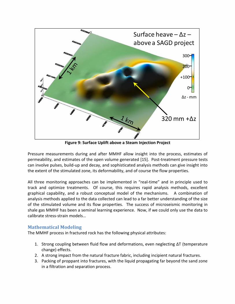
In Figure 8, several important aspects of deformation monitoring are shown or implied. First, because the strains are actually very small in the overburden (but not necessarily in the process zone), the strains from the zone being stimulated are transmitted into the surrounding strata elastically, showing up as deformations (or tilts) at the surface. This deformation field can be sampled at many points at the surface, and this can be analyzed to give information about the process at depth. Figure 8 shows that the complex deformation in the bottom half is the elastic sum of the deformations arising from a locus of pure volume change (a nucleus-of-strain [13]) and a line of defined shear displacement (a displacement discontinuity). In principle, with good data, it is possible to mathematically solve for a number of these “kernels” at depth in the stimulated region, building up a picture of what is happening in real time if the deformations (or tilts) can be collected in real time. Figure 9 is a vertical deformation image above a steam injection operation. This scenario is different than hydraulic fracturing stimulation, but the principle is the same: shear and volume changes at depth generate a surface deformation field that in principle can be analyzed mathematically to deconvolve deformations at depth [14].

Surface heave – Δz –above a SAGD project

320 mm +Δz

300

+100

200

0

Δz - mm

Figure 9: Surface Uplift above a Steam Injection Project

Pressure measurements during and after MMHF allow insight into the process, estimates of permeability, and estimates of the open volume generated [15]. Post-treatment pressure tests can involve pulses, build-up and decay, and sophisticated analysis methods can give insight into the extent of the stimulated zone, its deformability, and of course the flow properties. All three monitoring approaches can be implemented in “real-time” and in principle used to track and optimize treatments. Of course, this requires rapid analysis methods, excellent graphical capability, and a robust conceptual model of the mechanisms. A combination of analysis methods applied to the data collected can lead to a far better understanding of the size of the stimulated volume and its flow properties. The success of microseismic monitoring in shale gas MMHF has been a seminal learning experience. Now, if we could only use the data to calibrate stress-strain models…

Mathematical Modeling The MMHF process in fractured rock has the following physical attributes:

1. Strong coupling between fluid flow and deformations, even neglecting ΔT (temperature change) effects.

2. A strong impact from the natural fracture fabric, including incipient natural fractures. 3. Packing of proppant into fractures, with the liquid propagating far beyond the sand zone

in a filtration and separation process.

4. Wedging open of fractures by sand permanently propping open induced, reopened or reactivated fractures near the wellbore.

5. Shear displacement across fractures and bedding planes, leading to self-propping. 6. Block displacement and elastic compression, as well as block rotations that cause

fracture apertures to open and slip, leading to enhanced and preserved fracture conductivity

7. Massive alterations in fracture permeability as the processes of wedging, shear and propping occur in a large region around the wellbore – the dilated zone.

These factors are just about as non-linear, complex and coupled as it is possible to be in practical geomechanics. The first need is to find what simplifications and averaging methods can be realistically employed without degrading the physics beyond recognition; too many “fudge” factors and too much large-scale averaging obscures the actual physical processes. However, as we know from decades of rock mechanics experience, often a simple model tells us what we need to know, and it may even be calibrated if appropriate measurements are available. We have a great deal to learn about history-matching and model calibration from petroleum reservoir engineers. Our ability to simulate these processes will nonetheless remain severely limited, even with simplifications and volume averaging. First, the ever-present issue of rock characterization is made doubly difficult because the rocks are 1-3+ km deep, closed and incipient fractures cannot be detected at depth between boreholes, and geophysical data are limited to low-resolution seismic methods supplemented by borehole data. Providing realistic fracture fabric attributes for deterministic simulations in realistic cases remains beyond our capability. Second, continuum mechanics simulators based on finite difference (FD), finite element (FEM), boundary element (BEM) and displacement discontinuity (DD) formulations experience severe mathematical difficulties in realistically analyzing actual fractured systems experiencing opening and closing of fracture apertures, propagating fractures along their length, block rotation, and the other non-linearities involved such as slip and self-propping. For example, how would you represent the massively changing permeabilities associated with block rotation and opening of a fracture plane of changing aperture between two blocks? Can this be done using volume averaging methods with a large “unit volume”? What functions do you propose? These are not trivial issues; FD, FEM, BEM and DD methods, alone or iteratively coupled (e.g., a FD reservoir simulator coupled with a BEM rock mechanics simulator), cannot handle the problem size and the discrete block physics involved. Third, can discrete element methods (DEM) come to our rescue? A discrete element code such as 3-DEC has exceedingly long execution times if massive numbers of blocks that are free to rotate are simulated. Furthermore, such codes require refinements to handle fluid flow in the fracture network with simultaneous sand emplacement (filtration-[7]) and matrix flow. How do you calculate the fluid transmission properties of a fracture that is wedged open and therefore has a varying aperture along its length? Can sand emplacement be treated entirely separately, simply generating an input file to the DEM simulator? What are the flow properties of a self-

propped shear-displacement fracture? These questions are almost irresolvable. Nevertheless, despite the difficulties involved, DEM methods offer hope in generating better MMHF models, but it is extremely unlikely that they will be used alone.

Fluid is injected through a vertical wellbore in the middle of the model consisting of an array of naturally existing unbonded fractures

Several hundred natural fractures were included in this model …. Size of the model 100’s of feet on each dimension (XYZ)

Courtesy Ivan Gil, Itasca Corp.

Figure 10: Three-Dimensional DEM Simulation of Hydraulic Injection into a Fractured Medium

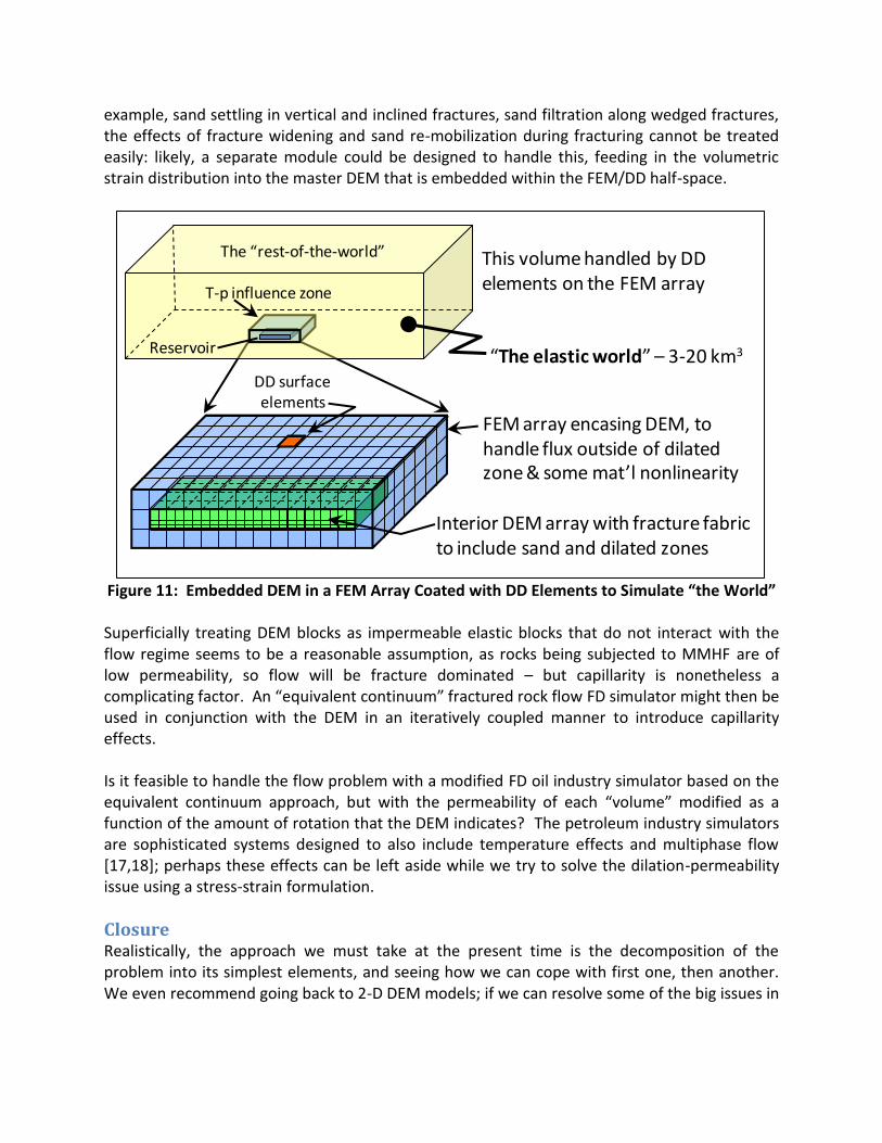
Figure 10 [16] shows a model that was developed to study the effects of viscosity and flow rate on the tendency of rocks to fail in shear along pre-defined joint planes, essentially one step toward solving the issue of shear and self-propping. If such models could have the actual flow capacity of the joint planes introduced as a function of aperture, rotation, etc., it would be another important step, but of course it would increase computational effort by an order of magnitude or more. Also, discretization of an entire representative continuum into discrete blocks is simply impossible because of the number of degrees of freedom involved. It may be best to imbed a DEM model within a FEM region that can handle the local stress changes and diffusive flux (p, T), and covered with DD elements to represent the half-space and introduce the far-field boundary conditions of stress and displacement. As long as the distant rock beyond the dilated zone acts elastically and without diffusive flux, it can be represented by continuum DD methods (Figure 11), reducing the degrees of freedom by a factor of 3 to 5, compared to FEM. The stiffness of the continuum part of the model can be modified to reflect the confining effects of the surroundings, and the active DEM embedment can be limited to a volume somewhat larger than the dilated zone. In the local dilated zone “permeability” can be linked to the strain, but the nature of the functionality remains uncertain because of the effect of block rotations. In principle this could be done tensorially as well, bringing in a more realistic component of anisotropic evolution of flow properties, but this is excessively optimistic. It will be more efficient to separate the various numerical “tasks” into different models whenever possible, combining the results in a time-stepping manner (iterative coupling). For

example, sand settling in vertical and inclined fractures, sand filtration along wedged fractures, the effects of fracture widening and sand re-mobilization during fracturing cannot be treated easily: likely, a separate module could be designed to handle this, feeding in the volumetric strain distribution into the master DEM that is embedded within the FEM/DD half-space.

DD surface elements

The “rest-of-the-world”

Reservoir

T-p influence zone

This volume handled by DD elements on the FEM array

Interior DEM array with fracture fabric to include sand and dilated zones

“The elastic world” – 3-20 km3

FEM array encasing DEM, to handle flux outside of dilated zone & some mat’l nonlinearity

Figure 11: Embedded DEM in a FEM Array Coated with DD Elements to Simulate “the World”

Superficially treating DEM blocks as impermeable elastic blocks that do not interact with the flow regime seems to be a reasonable assumption, as rocks being subjected to MMHF are of low permeability, so flow will be fracture dominated – but capillarity is nonetheless a complicating factor. An “equivalent continuum” fractured rock flow FD simulator might then be used in conjunction with the DEM in an iteratively coupled manner to introduce capillarity effects. Is it feasible to handle the flow problem with a modified FD oil industry simulator based on the equivalent continuum approach, but with the permeability of each “volume” modified as a function of the amount of rotation that the DEM indicates? The petroleum industry simulators are sophisticated systems designed to also include temperature effects and multiphase flow [17,18]; perhaps these effects can be left aside while we try to solve the dilation-permeability issue using a stress-strain formulation.

Closure Realistically, the approach we must take at the present time is the decomposition of the problem into its simplest elements, and seeing how we can cope with first one, then another. We even recommend going back to 2-D DEM models; if we can resolve some of the big issues in

2-D, we can move on to 3-D. Jumping immediately to a 3-D formulation may lead to excessively difficult interactions because of the massive non-linearities involved. Whatever direction turns out to be the best, there are several factors to remember: the economic impact of better MMHF simulation is huge, given the trillions of dollars of resources involved; also, no progress will be made without monitoring and the use of good quality data to calibrate and verify models. There is considerable value remaining in the concept of calibrated models that are simplified, but robust enough that they can be used in subsequent analyses of a predictive nature. This is in the best spirit of our discipline: do “hard” analysis when we can and when it is of benefit, use common sense and simplifications as we must to address real-world issues. That is what applied petroleum geomechanics is all about: solving real problems as best we can, given the great complexity of the processes, while also recognizing technical and socio-economic-environmental issues [19].

1. http://oilshalegas.com/montereyshale.html 2. Carlisle, P.H. (2003). The attributes of a Wolfcamp “Reef” play, Pecos County, Texas.

Search and Discovery Article #10037. 3. El Ela, M.A., Samir, M., Sayyouh, H. and El-Tayeb, S. (2008). Thermal heavy-oil recovery

projects succeed in Egypt, Syria. Oil & Gas Journal, 106(48), December 22 issue. 4. Bunger, A.P., Jeffrey, R.G. and Detournay, E. (2008). Evolution and morphology of

saucer-shaped sills in analogue experiments. Geological Society London, Special Publications; 2008; v. 302; p 109-120.

5. Bray, J.W. and Goodman, R.E. (1981). The theory of base friction models. International Journal of Rock Mechanics and Mining Sciences & Geomechanics Abstracts, 18(6), 453-468.

6. Ladanyi, B. and Archambault, G. (1970). Simulation of shear behaviour of a jointed rock mass. In: Rock Mechanics – Theory & Practice, Proc. 11th Symp. Rock Mech., pp 105-125, New York: American Institute of Mining, Metallurgical and Petroleum Engineers.

7. Xia, G.W., Dusseault, M.B. and Marika, E. (2007). A hydraulic fracture model with filtration for biosolids injection. Proc 1st Canada-U.S. Rock Mech. Symp., Paper 061, 8 p.

8. Cipolla, C.L., Lolon, E.P., Erdle, J.C. and Rubin, B. (2010). Reservoir modeling in shale-gas reservoirs. SPE Reservoir Engineering and Evaluation J., 13(4), 638-653.

9. Wiles, T. and MacDonald, P. (1988). Correlation of stress analysis results with visual and microseismic monitoring at Creighton Mine. Computers and Geotechnics, 5, 105-121.

10. Board, M.P. (1994). Numerical examination of mining-induced seismicity. Ph.D. Thesis, University of Minnesota, Minneapolis, MN, 240 pp.

11. Urbancic, T.I. and Trifu, C-I. (2000). Recent advances in seismic monitoring technology at Canadian mines, Journal of Applied Geophysics, 45, pp. 225-237.

12. Zimmer, U., Maxwell, S.C., Waltman, C.K. and Warpinski, N.R. (2009). Microseismic monitoring quality control (QC) reports as an interpretative tool for nonspecialists. SPE 110517, SPE J., Vol. 14, Number 4, December, pp. 737-745.

13. Geertsma, J. (1973). Land subsidence above compacting oil and gas reservoirs. SPE 3730, JPT, June.

14. Dusseault, M.B. and Simmons, J.V. (1982). Injection-induced stress and fracture orientation changes. Can. Geot. J., 19, 4, pp. 482-493.

15. Barree, R.D., Barree, V.L. and Craig, D. (2009). Holistic fracture diagnostics: consistent interpretation of prefrac injection tests using multiple analysis methods. SPE 107877, SPE Production & Operations, Volume 24, Number 3, August, pp. 396-406.

16. Damjanac, B., Gil, I., Pierce, M., Sanchez, M., Van As, A. and McLennan, J. (2010). A new approach to hydraulic fracturing modeling in naturally fractured reservoirs. Proc. American Rock Mechanics Association Annual Conference, Paper ARMA 10-400.

17. McLennan, J. Tran, D., Zhao, N., Thakur, S., Deo, M., Gil, I. and Damjanac, B. (2010). Modeling fluid invasion and hydraulic fracture propagation in naturally fractured formations: a three-dimensional approach. SPE 127888, SPE Intl. Symp. And Exhib. on Formation Damage Control, February 10-12, Lafayette, LA.

18. Cipolla, C.L., Williams, M.J., Weng, X., Mack, M. and Maxwell, S. (2010). Hydraulic fracture monitoring to reservoir simulation: maximizing value. SPE 133877. SPE ATCE, Florence, Italy, Sept. 19-22.

19. Zoback, M., Kitaseib, S. and Copithorne, B. (2010). Addressing the environmental risks from shale gas development. Briefing Paper 1, Worldwatch Institute, Natural Gas and Sustainable Energy Initiative. July.