30
K. Salah 1 2. Review of Probability and Statistics Refs: Law & Kelton, Chapter 4
| Date post: | 02-Jan-2016 |
| Category: |
Documents |
| Upload: | cody-evans |
| View: | 219 times |
| Download: | 0 times |

K. Salah 1
2. Review of Probability and Statistics
Refs: Law & Kelton, Chapter 4
K. Salah 2
Random Variables
•Experiment: a process whose outcome is not known with certainty
•Sample space: S = {all possible outcomes of an experiment}
•Sample point: an outcome (a member of sample space S)
•Example: in coin flipping, S={Head,Tail}, Head and Tail are outcomes
•Random variable: a function that assigns a real number to each point in sample space S
•Example: in flipping two coins:
•If X is the random variable = number of heads that occur
•then X=1 for outcomes (H,T) and (T,H), and X=2 for (H,H)
K. Salah 3
Random Variables: Notation
•Denote random variables by upper case letters: X, Y, Z, ...
•Denote values of random variables by lower case letters: x, y, z, …
•The distribution function (cumulative distribution function) F(x) of random variable X for real number x is
F(x) = P(Xx) for -<x<
where P(Xx) is the probability associated with event {Xx}
F(x) has the following properties:
0F(x) 1 for all x
F(x) is nondecreasing: i.e. if x1x2 then F(x1) F(x2)
0)(lim1)(lim
xFandxFxx

K. Salah 4
Discrete Random Variables
•A random variable is discrete if it takes on at most a countable number of values
•The probability that random variable X takes on value xi is given by:
p(xi) = P(X=xi) for I=1,2,…
and
p(x) is the probability mass function of discrete random variable X
F(x) is the probability distribution function of discrete random variable X
1)(1
iixp
xallforxpxFxx
i
i
)()(

K. Salah 5
Continuous Random Variables
X is a continuous random variable if there exists a non-negative function f(x) such that for any set of real numbers B,
f(x) is the probability density function for the continuous RV X:
F(x) is the probability distribution function for the continuous RV X:
1)(
)()(
dxxfand
dxxfBXPB
0)(]),[()(: x
x
dyyfxxXPxXPNote
xallfordyyfxXPxFx
)(]),[()(

K. Salah 6
Distribution and density functions of a Continuous Random Variable
Given an interval I = [a,b]
)()()()( aFbFdyyfIXPb
a
b
a
dyyfbxaP )()(
a b x
f(x)

K. Salah 7
Joint Random Variables
In the M/M/1 queuing system, the input can be represented as two sets of random variables:
arrival times of customers: A1, A2, …, An
and service times of customers: S1, S2, …, Sn
The output can be a set of random variables:
delays in queue of customers: D1, D2, …, Dn
The D’s are not independent.
K. Salah 8
Jointly discrete Random Variables
Consider the case of two discrete random variables X and Y,
the joint probability mass function is
p(x,y) = P(X=x,Y=y) for all x,y
X and Y are independent if
p(x,y) = pX(x)pY(y) for all x,y
these are the marginal probability mass functions
xallY
yallX
yxpypand
yxpxpwhere
),()(
),()(

K. Salah 9
Jointly continuous Random Variables
Consider the case of two continuous random variables X and Y.
X and Y are jointly continuous random variables if there exists a non-negative function f(x,y) (the joint probability density function of X and Y) such that for all sets of real numbers A and B,
X and Y are independent if
fX(x) and fY(y) are called the marginal probability density functions
B A
dxdyyxfBYAXP ),(),(
dxyxfyfand
dyyxfxfwhere
yxallforyfxfyxf
Y
X
YX
),()(
),()(
,)()(),(
K. Salah 10
Measuring Random Variables: mean and median
Consider n random variables X1, X2, …, Xn
The mean of the random variable Xi (i=1,2,…,n) is
iX
jijXj
i
Xcontinuousfordxxfx
Xdiscreteforxpx
i
i
)(
)(1
The mean is the expected value, and is a measure of central tendency.
The median, x0.5 , is the smallest value of x such that FX(x) 0.5
For a continuous random variable, F(x0.5) = 0.5
K. Salah 11
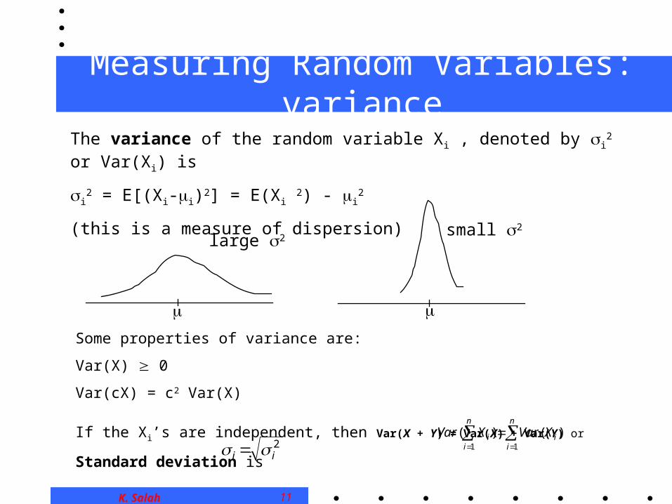
Measuring Random Variables: variance
The variance of the random variable Xi , denoted by i2 or Var(Xi) is
i2 = E[(Xi-i)2] = E(Xi 2) - i
2
(this is a measure of dispersion)
large 2 small 2
Some properties of variance are:
Var(X) 0
Var(cX) = c2 Var(X)
If the Xi’s are independent, then Var(X + Y) = Var(X) + Var(Y) or Standard deviation is
n
ii
n
ii XVarXVar
11
)()(2ii

K. Salah 12
Variance is not dimensionlessService time (min) Service time (sec)
0.142865181 8.571910860.290269546 17.416172750.948536714 56.912202850.054366311 3.2619786470.790397379 47.423842720.703983277 42.238996640.031094127 1.8656476380.58675124 35.205074390.695252758 41.715165490.288665663 17.319939760.196799289 11.807957310.977139718 58.628383070.700495571 42.029734240.778327141 46.699628470.16218063 9.7308377970.987293722 59.237623320.422970857 25.378251410.208112375 12.48674250.082961343 4.9776805770.974676034 58.480562030.120347847 433.25225 Variance0.501156944 30.06941662 Mean
*602
*60
e.g. if we collect data on service times at a bank machine with mean 0.5 minutes, variance 0.1 minute,
the same data in seconds will give mean 30 seconds, variance 360 seconds;
i.e., variance is dependent on scale!

K. Salah 13
Measures of dependenceThe covariance between random variables Xi and Xj where i=1,…,n and j=1,…,n is
Cij = Cov(Xi , Xj) = E[(Xi - i)(Xj- j)] = E[Xi Xj] - i j
Some properties of covariance:
Cij = Cji
if i=j, then Cij = Cji = Cii = Cjj = i2
if Cij > 0, then Xi and Xj are positively correlated:
Xi > i and Xj > j tend to occur together,
and Xi < i and Xj < j tend to occur together
if Cij < 0, then Xi and Xj are negatively correlated:
Xi > i and Xj < j tend to occur together,
and Xi < i and Xj > j tend to occur together
Cij is NOT dimensionless, i.e. the value is influenced by the scale of the data.
K. Salah 14
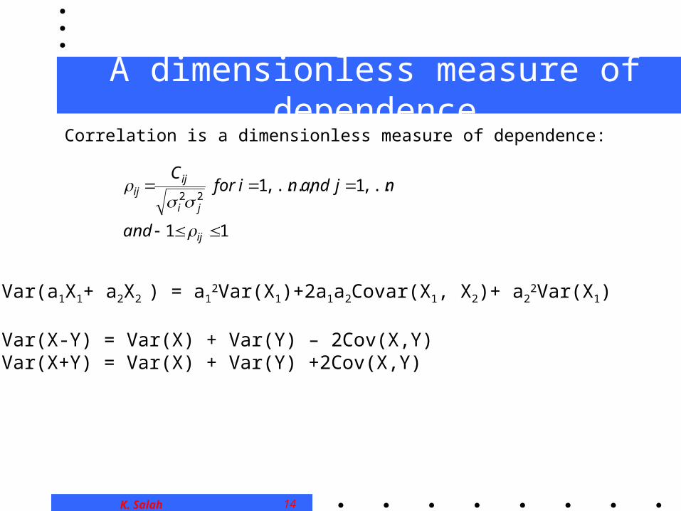
A dimensionless measure of dependenceCorrelation is a dimensionless measure of dependence:
11
,...,1,...,122
ij
ji
ijij
and
njandniforC
Var(a1X1+ a2X2 ) = a12Var(X1)+2a1a2Covar(X1, X2)+ a2
2Var(X1)
Var(X-Y) = Var(X) + Var(Y) – 2Cov(X,Y)Var(X+Y) = Var(X) + Var(Y) +2Cov(X,Y)
15
The covariance between the random
variables X and Y, denoted by Cov(X, Y), is
defined by
Cov(X, Y) = E{[X - E(X)][Y - E(Y)]}
= E(XY) - E(X)E(Y)
The covariance is a measure of the
dependence between X and Y. Note that
Cov(X, X) = Var(X).

16
Definitions:
Cov(X, Y) X and Y are
= 0 uncorrelated
> 0 positively correlated
< 0 negatively correlated
Independent random variables are also uncorrelated.
17
Note that, in general, we have
Var(X - Y) = Var(X) + Var(Y) -
2Cov(X, Y)
If X and Y are independent, then
Var(X - Y) = Var(X) + Var(Y)
The correlation between the random
variables X and Y, denoted by Cor(X, Y),
is defined by
Cov( )Cor( )
Var( )Var( )
X ,YX ,Y
X Y

18
It can be shown that
-1 Cor(X, Y) 1

19
4.2. Simulation Output Data and Stochastic Processes
A stochastic process is a collection of "similar" random variables ordered over time all defined relative to the same experiment. If the collection is X1, X2, ... ,
then we have a discrete-time stochastic process. If the collection is {X(t), t 0}, then we have a continuous-time stochastic process.

20
Example 4.3: Consider the single-server queueing system of Chapter 1 with independent interarrival times A1, A2, ... and independent processing times P1, P2, ... . Relative to the experiment of generating the Ai's and Pi's, one can define the discrete-time stochastic process of delays in queue D1, D2, ... as follows:
D 1 = 0
Di +1 = max{Di + Pi - Ai +1, 0} for i = 1, 2, ...
21
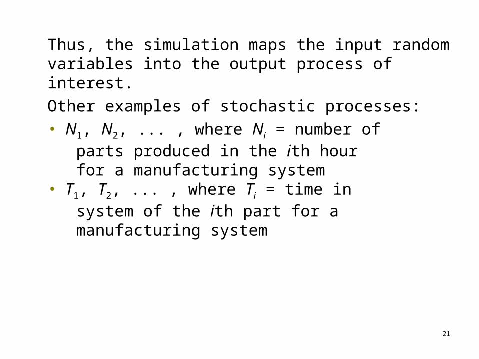
Thus, the simulation maps the input random variables into the output process of interest.
Other examples of stochastic processes:
• N1, N2, ... , where Ni = number of parts produced in the ith hour for a manufacturing system• T1, T2, ... , where Ti = time in system of the ith part for a manufacturing system
22
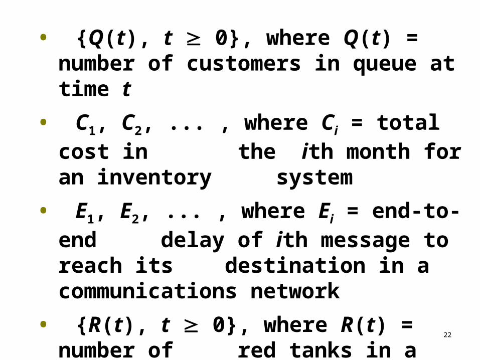
• {Q(t), t 0}, where Q(t) = number of customers in queue at time t
• C1, C2, ... , where Ci = total cost in the ith month for an inventory system
• E1, E2, ... , where Ei = end-to-end delay of ith message to reach its destination in a communications network
• {R(t), t 0}, where R(t) = number of red tanks in a battle at time t
23
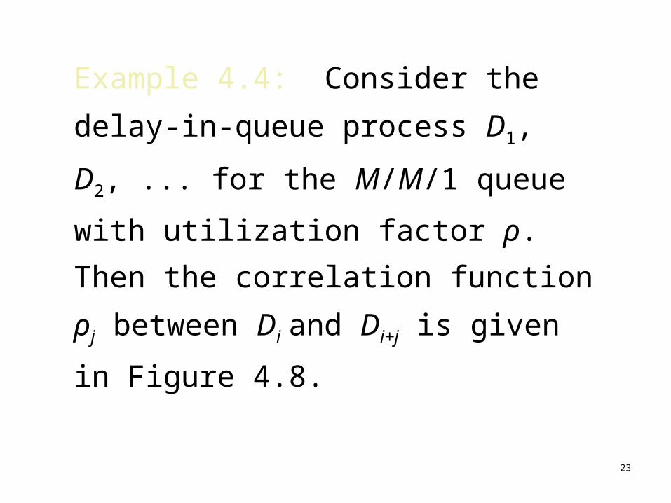
Example 4.4: Consider the delay-in-
queue process D1, D2, ... for the M/M/1
queue with utilization factor ρ. Then
the correlation function ρj between Di
and Di+j is given in Figure 4.8.

24
1.0
0.9
0.8
0.7
0.6
0.5
0.4
0.3
0.2
0.1
0 1 2 3 4 5 6 7 8 9 10j
ρj
Figure 4.8. Correlation function ρj of the process D1, D2, ... for the M/M/1 queue.
ρ = 0.9
ρ = 0.5
K. Salah 25
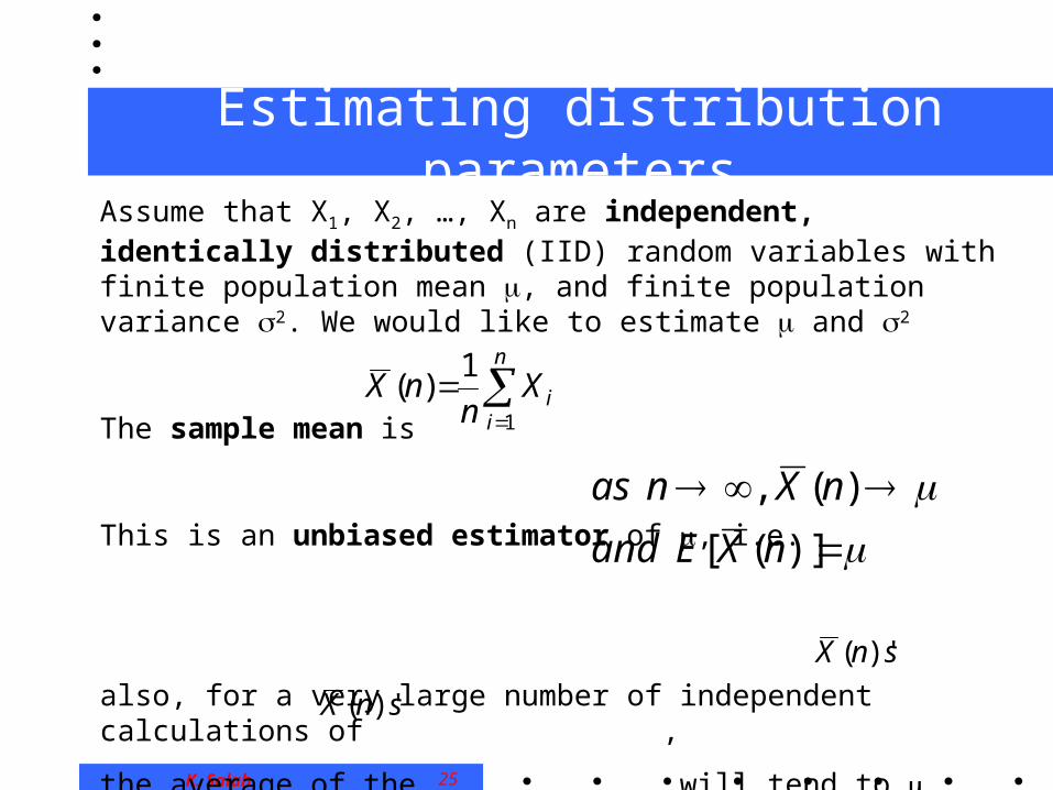
Estimating distribution parametersAssume that X1, X2, …, Xn are independent, identically distributed (IID) random variables with finite population mean , and finite population variance 2. We would like to estimate and 2
The sample mean is
This is an unbiased estimator of , i.e.
also, for a very large number of independent calculations of ,
the average of the will tend to
n
iiXn
nX1
1)(
)]([
)(,
nXEand
nXnas
snX )'(
snX )'(

K. Salah 26
Estimating varianceThe sample variance is
This is an unbiased estimator of , i.e. E[s2(n)] = 2
this is a measure of how well estimates
2
1
2 )]([1
1)( nXX
nns
n
ii
nnXVar
2
)]([
)(nX
n
ii nXX
nnns
nnXarV
isnXVarofestimateAn
1
22 )]([)1(
1)(
1)]([ˆ
))((

K. Salah 27
Two interesting theoremsCentral Limit Theorem:
For large enough n, tends to be normally distributed with mean and variance 2/n
This means that we can assume that the average of a large numbers of random samples is normally distributed - very convenient.
Strong Law of Large Numbers:
For an infinite number of experiments, each resulting in , for sufficiently large n, will be arbitrarily close to for almost all experiments.
This means that we must choose n carefully: every sample must be large enough to give a good .
)(nX
)(nX )(nX
)(nX

K. Salah 28
0.0 1.0 2.0 3.00.0-1.0-2.0-3.00.00
0.05
0.10
0.15
0.20
0.25
0.30
0.35
Area = 0.68
x
f x( )
Figure 4.7. Density function for a N(, 2) distribution.

K. Salah 29
Confidence Intervals
n
nsz(n)X
)(
isforintervalconfidence)%1(100A
2
21
0x
21
z
21
z
f(x) 1-
Interpretation of confidence intervals:
If one constructs a very large number of independent 100(1-)% confidence intervals, each based on n observations, with n sufficiently large, then the proportion of these confidence intervals that contain should be 1-.
What is n sufficiently large?
The more “non-normal” the distribution of Xi , the larger n must be to get good coverage (1- ).

K. Salah 30
An exact confidence intervalIf the Xi’s are normal random variables, then tn has a t distribution with n-1 degrees of freedom (df), and an exact 100(1-)% confidence interval for is:
This is better than z’s confidence interval, because it provides better coverage (1- ) for small n, and converges to the z confidence interval for large n.
Note: this estimator assumes that the Xi’s are normally distributed. This is reasonable if the central limit theorem applies: i.e. each Xi is the average of one sample (large enough to give a good average), and we take a large number of samples (enough samples to get a good confidence interval).
n
nst(n)Xn
)(2
21,1


