00 CO CO 00

Q

FIFTH SEMIANNUAL TECHNICAL REPORT

(15 December 1971 - 15 June 1972)

FOR THE PROJECT

"RESEARCH IN

STORE AND FORWARD COMPUTER NETWORKS"

Principal Investigator

and Project Manager:

HOWARD FRANK (516) 671-9580

ARPA Order No. 1523

Contractor: Network Analysis Corporation

Contrrct No. DAHC 15-70-C-0120

Effective Date: 15 October 1969

Expiration Date: 1? October 1972

NATIONAl TECHNICAL INFORMATION SERVICE

Sponsored by

Advanced Research Projects Agencjr

Department of Defneae

D D C jllZl2EDrii2E

SEP 14 .972

ulkiSEircrEJ B

DISTRIBUTION STATEMENT A

Appioved for public reloc»«; Diatrlbutjon Unlimited

The views and conclusions contained \n this document are those of the authors and should not be interpreted as necessarily representing the official policies, either expressed or implied, of the Advanced. Research Projects Agency or tho IKS. Government»

^3

...

THIS DOCUMENT IS BEST QUALITY AVAILABLE. THE COPY

FURNISHED TO DTIC CONTAINED A SIGNIFICANT NUMBER OF

PAGES WHICH DO NOT · REPRODUCE LEGIBLY.

DOCUMEMT CO.STfCOL DATA - r<o.D

\. w^ni.NATtNC. ACTIVITY •'•7«rj*Wal« «uilMilj

Network Analysis Corporation 3eochwcod,01a Tappan Rd.,Gien Cove#NY **' &H0,^,nc

Scniannual Ropct No. 5 June 1972

• . iwUC"> ^*lVi NJ*«i jTiV» t/rfpvi »ni <nc«u»^« »i«i«»i

Semiannual Technical Report, 15 rec. ^971 - 15 June 1972

Network Analysis Corporation

ft. «W^WNT i.*~i.

June 1972 1m TOTA» .O. Of PAi£Ä 7b. NO. i ^ Hfcfi

91 27

DAKC-1-.-70-C-G120 -. ^Ad«CCT NC.

ARPA Order No. 1523

I ARPA SEMIANNUAL REPORT NO.

,Ji. AV*.»Ae.».«TV/toiMiTAT.ON NOTlCti

Tr.i» wwCwT.'.crti hi» beer« apprwvcci föf pubUc rclcasti -»ü iaic; U» di»».*i>uUon is unUsiiStf««

■.l. ÄwAt'fci.Vt.fvT A»»Y KOTL»

Nvr.c\ \

[u. A.iTiiAct Thia report studies rellabiliuy prcperuies of store-and- \ 'forward networks, analysis of neuwork reliability and algoriahr^s for niinimum spanning trees. A study of the tradeoffs between network size, connectivity, and component reliability shows tnat large networks re- liability will be a major, and perhc,p- dominant, design problem. :Recursive analysis techniques for loop and tree combinatio..- greatly »reduce analysis cost, while improved methods for generating minimum spanning trees have a similar effect for this fundamental network problem.

,4. Akt m^Hi,*

Computer networks, throughput, cost, reliability, Ai<?A Computer Network, store-anu-^orw^rd

survivab^.... ly,

TABLE OF CONTENTS

Page

I. RELIABILITY AND LARGE COMPUTER NETWORKS 1

1. Introduction and Summary. * 1 2. Reliability of Small to Medium Networks(NN=50) 5 3. Reliability Trends for Large Networks -.12 4. Implications for Further Research 21

II, RECURSIVE ANALYSIS NETWORK RELIABILITY 23

1. Introduction and Summary , 23 2. Terminology 4 25 3. Recursive Computation on Trees «.. oq

4. Trees with Weighted Nodea > 5. Extension to General Networks 38 6. Point of Evaluation versus Functional Evaluation 42

III. A NEW ALGORITHM FOR MINIMUM SPANNING TREE CALCULATIONS .* .48

1. Introduction and Summary 48 2. A History of Minimum Spanning Tree Calculations 53 3. Finding Components of a Graph and Spanning Forests ^.%. .56 4. New Developments in MST Calculation ...60 5. Numerical Experiments * 63 6. Summary and Conclusion 68

IV. REFERENCES 86

2

SUMMARY

Technical Problem

The Network Aiialysis Corporation contract with the Advanced

Research Projects Agency incorporates the following objectives;

To determine the most economical cCitfigurations for the ARPANET,

to study the properties of store and forward networks and to de-

velop procedures for analysis and design of reliable computer

communication networks.

General Methodology

The heart of the research program has been a dual attack on

basic network theoretical problems and the development of compu-

tational techniques for the study of large networks.

Technical Results

Some of the results accomplished during the reporting period

are:

• A study of the tradeoffs between network size, network

connectivity and component reliability was completed.

This study indicates that reliability will be a major

and perhaps dominant issue for large network design.

3

• A new method for reliability analysis which uses a

recursive technique has been developed to handle a

large class of networks composed of loops and trees.

This method allows a wide variety of reliability

criteria to be evaluated simultaneously at a small

fraction of the c\>st of previously known methods,

• New and improved computational techniques for finding

"minimum spanning trees \ (a fundamental network

problem) were derived. This computation is a basic

ingredient in many large scale network algorithms.

Department of Defense Implications

Communication networks for meeting Department of Defense

requirements involve huge network structures that present tech-

niques are inadequate to handle. The results of the reporting

period highlight the role that reliability will play in such

networks, provide new techniques fCi. ehe analysis of large

Defense Department networks and meet some of the computational

requirene nts for xarge scale network cesign.

Implications for Further Research

This report shows that for very Jaxge networks, cost/

reliability considerations rnus^ be given equal importance to

cost/throughput considerations. Thii* means that there will be

a need to develop dramatically different network design procedures

tc insure availability of resources in a large network. The re-

quirements of the new procedures, while not yet well defined,

indicate that computation breakthroughs for a number of basic

network problems will be necessary.

t ■ i)

I. RELIABILITY AND LARGE COMPUTER NETWORKS

1. Introduction and Summary

The major considerations in the system design of a computer

network such as the ARPANET are:

1) Cc&t

2) Throughput

3) Delay and response time

4) Network reliability

While it is essential to consider each of these constraints,

it often results that several are automatically satisfied for

designs satisfying the remaining. Initially, this was the

case i.'or the ARPANET. The delay and response t ime was ade-

quately considered by slightly derating the line capacities

of the 50 kilobit links and the reliability was adequate if

there were at least two node disjoint paths between each pair

of nodes. Thus, the cost-throughput tradeoff was the over-

riding consideration. Given these conditions, it is possible

to design very efficient networks in a reasonable amount of

compucing time. However, it is becoming evident that as the

ARPANET increases in size, the reliability constraints are

beginning to limit design choicef». It may even become that

the cost-reliability tradeoff may replace the cost-throughput

tradeoff as the basic design consideration. While for small

versions of the ARPANET^ any design with at least two node

disjoint paths between each node pair and sufficient through-

put would necessarily be reliable enough, initial investigations

indicate that for large networks sufficient reliability auto-

matically implies sufficient throughput. In any case, it is

clear that reliability constraints will play an ever increas-

ing role in the design process as the ARPANET becomes larger.

Considering this, it is quite sobering to note that many

large communication nutwo/ks are being designed

with little consideration of network reliability (as distin-

guished from component or element reliability).

R3liability analysis of computer networks is concerned

with the dependence of the reliability of the network on the »

reliability or its nodes and links. Element reliability is

easily definid as, for example, the fraction of time tha

element is operable, or as by the mean time between failures

and expected repair time. The proper measure of network re-

liability is not as clear and simple. Several possible

measures are: the number of elements which must be removed

to disconnect the network, the probability that the network

will be disconnected, the expected fraction of node pairs

which can communicate through the network, and the expected

throughput of the network subject to element failures. The above

measures are listed in order of their computational complexity.

Many other measures can and have been suggested. A whole other

class of measures arise when the nodes are not of equal importance.

as in centralized networks or hierarchai networks. In a centralized

network, one may be interested in the expected number of nodes which

can communicate with a central node. More general criteria arise

when different node pairs are weighted by their importance. For

example, communication between ILLIAC IV and' certain other nodes

will be of high priority in tne ARPANET. Most of our analysis

will deal with exepcted fraction of node pairs communicating al-

though in many cases any of the other criteria mentioned could

be used.

Node failures can affect network reliability in two ways.

First, if a node fails, clearly it cannot communicate with any

other iiOde In the network. Thus, if there are NN nodes in the

network a d one fails, a minimum of NN-1 node pairs cannot com-

municate independent of the network structure. In the next

section we establish a simple formula for measuring this effect.

Changing the network ^onfiguratior. has no effect on this com-

ponent of network reliability. Another effect of node failures

is that the failed 'es destroy some potential communication

paths between other pairs of nodes. Link failures also affect

network reliability in the second way.

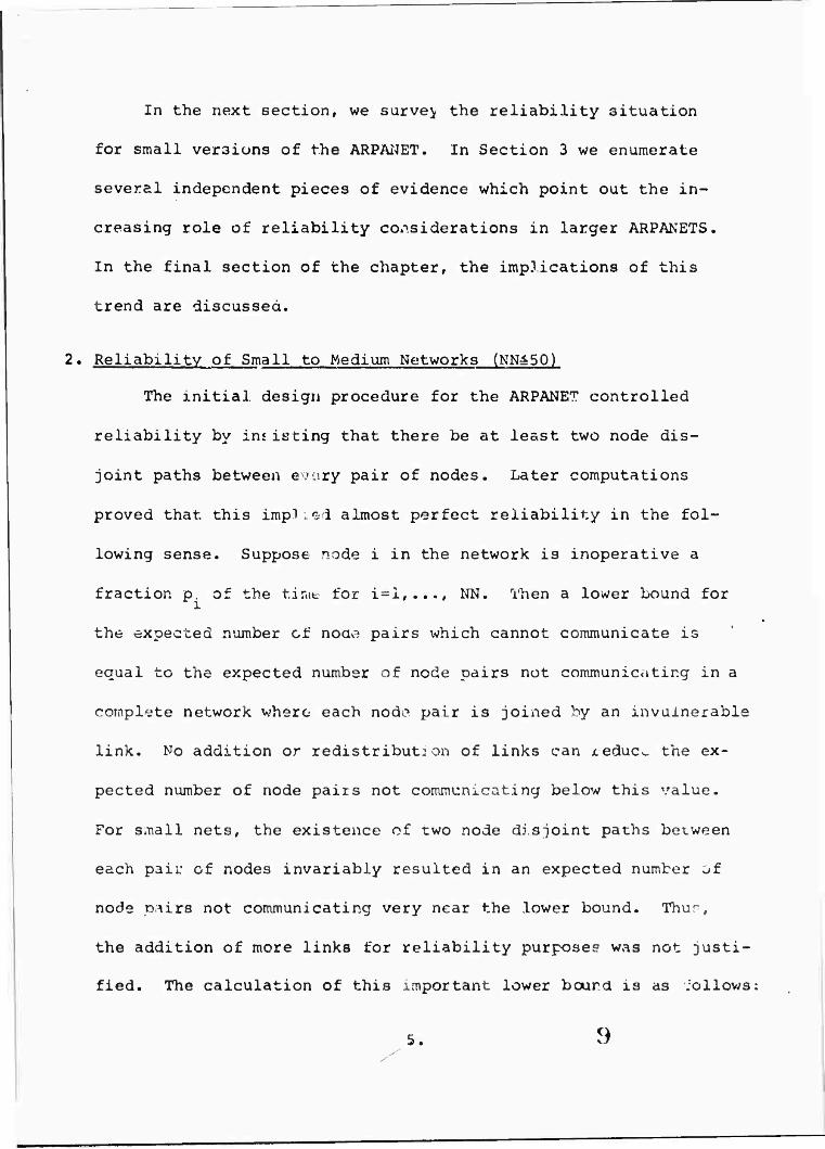
In the next section, we survey the reliability situation

for small versions of the ARPANET. In Section 3 we enumerate

several independent pieces of evidence which point out the in-

creasing role of reliability considerations in larger ARPANETS.

In the final section of the chapter, the implications of this

trend are discussed.

2. Reliability of Small to Medium Networks (NN^5Q)

The initial design procedure for the ARPANET controlled

reliability by im isting that there be at least two node dis-

joint paths between evi\ry pair of nodes. Later computations

proved that this implied almost perfect reliability in the fol-

lowing sense. Suppose node i in the network is inoperative a

fraction p. of the tirut for i=l,..., NN. Then a lower bound for i

the expected number of noae pairs which cannot communicate is

equal to the expected number of node pairs not communicating in a

complete network where each node pair is joined by an invulnerable

link. No addition or redistribution of links can xeduc^ the ex-

pected number of node pairs not communicating below this value.

For small nets, the existence of two node disjoint paths between

each pair of nodes invariably resulted in an expected number of

node pairs not communicating very near the lower bound. Thur#

the addition of more links for reliability purpose? was not justi-

fied. The calculation of this important lower bourd is as .follows:

5.

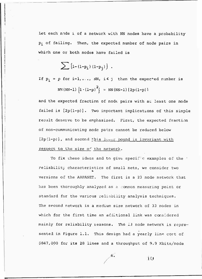
Let each node i of a network with NN nodes have a probability

Pj^ of failing. Then, the expected number of node pairs in

which one or both nodes have failed is

X^-d-PiHl-Pj)) •

If Pi = P for i=l#...# NN, i< j then the expected number is

NN(NN-l) |l-(l-p)2| = NN(NN-l) [2p(l-p)l

and the expected fraction of node pairs with at least one node

failed is [2p(l-p)]. Two important implications of this simple

result deserve to be emphasized. First, the expected fraction

of non-communicating node pa\rs cannot be reduced below

[2p(l-p)], and second this lower bound is invariant with

respect to the size or the network.

To fix these ideas and to give specif c examples Oic the '

reliability characteristics of small nets, we consider two

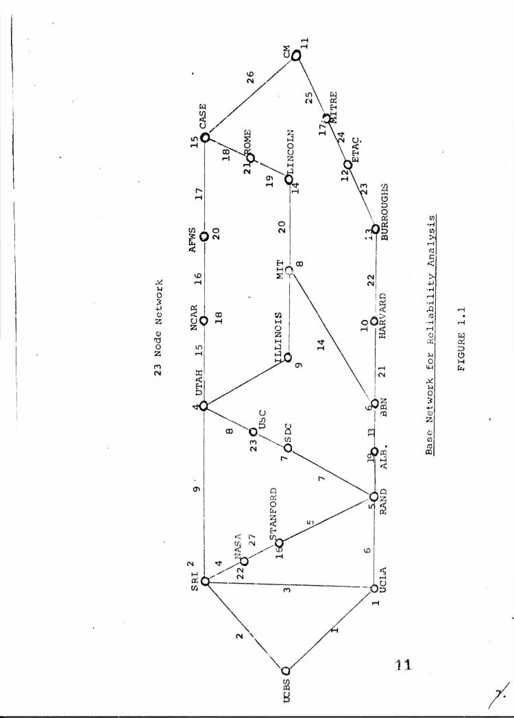
versions of the ARPANET. The first is a 23 node network that

has been thoroughly analyzed as a jommon measuring point or

standard for the various reliability analysis techniques.

The second network is a medium size network of 33 nodes in

which for the first time an additional link was considered

mainly for reliability leasons. Th6 13 node network is repre-

sented in Figure 1.1. This design had a yearly line cpet of

$847,000 for its 28 lines and a throughput of 9.9 Kbits/node

X- i(j

u O

0)

Q

rH C c

■H H •H

n •H H

OS

o

o ->

4-» QJ

(fl

PQ

D O H

11

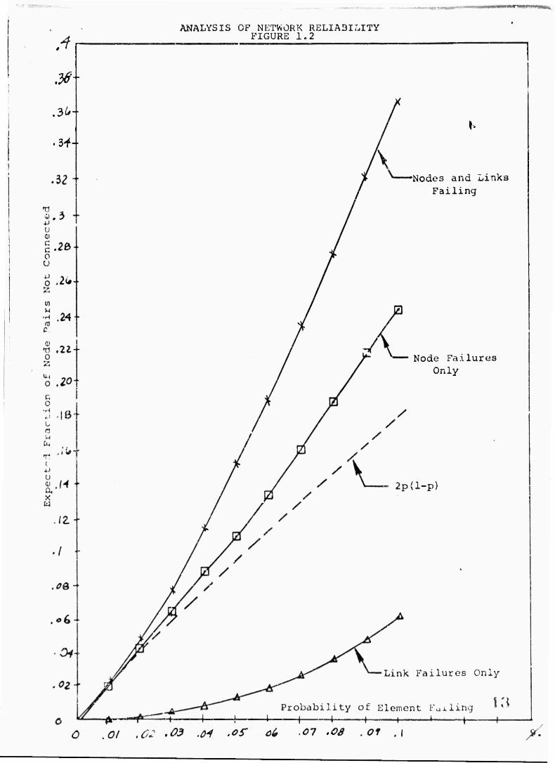
assuming uniform traffic between nodes. We will assume a

base element failure probability 0.02 which is a close

approximation to currently measured values. Then^ 2p(l-p)

equals 0.0395 for p=.01 and hence the expected fraction of

node pairs not communicating must be at least (.0396) (23) (22)/2

equals 10.0188. In Figure i.2 the expected fraction of node

pairs not communicating as a function of element failure

probability is shown. Also r.hown is the expected fraction

of node pairs not communxcating when only links fail, when only

nodes fail and finally when the curve 2p(l-p) is plotted.

For p = .02, the expected fraction of node pairs not communi-

cating is 0.04^.

In t>e case whore only nodes fail the e>.pect2d fraction

is .0427 and for only links failing .0018. Rem.r.herinr' that .

2p(i-p) = ,03 96, we .see that 80% of the node pairs which cannot

communicate can be ascribed to purely the fact that one of

the nodes of the pair in question has failed. Thus, the

improvement in reliability to be gained by chenging the network

configuration is miner. Nevertheless, ?everöl strateg.es for

improving reliability were examined. The most vulnerable

section of the 23 node network is the long string of nodes

from node 6 xBBN) to node 15 (CASE) along the bottom of

Figure 1.1. The firet idna wa«» to add a link from node 13

ANALYSIS OF NETWORK RELIABILITY FIGURE l^

.Of

Nodes and Linka Failing

Node Failures Only

1-p)

Link Failures Only

Probability of Element Fueling \ 1 1 1 1 \ H-

\:\

02 .03 .M .o? ob '01 '0ß '0f -' X-

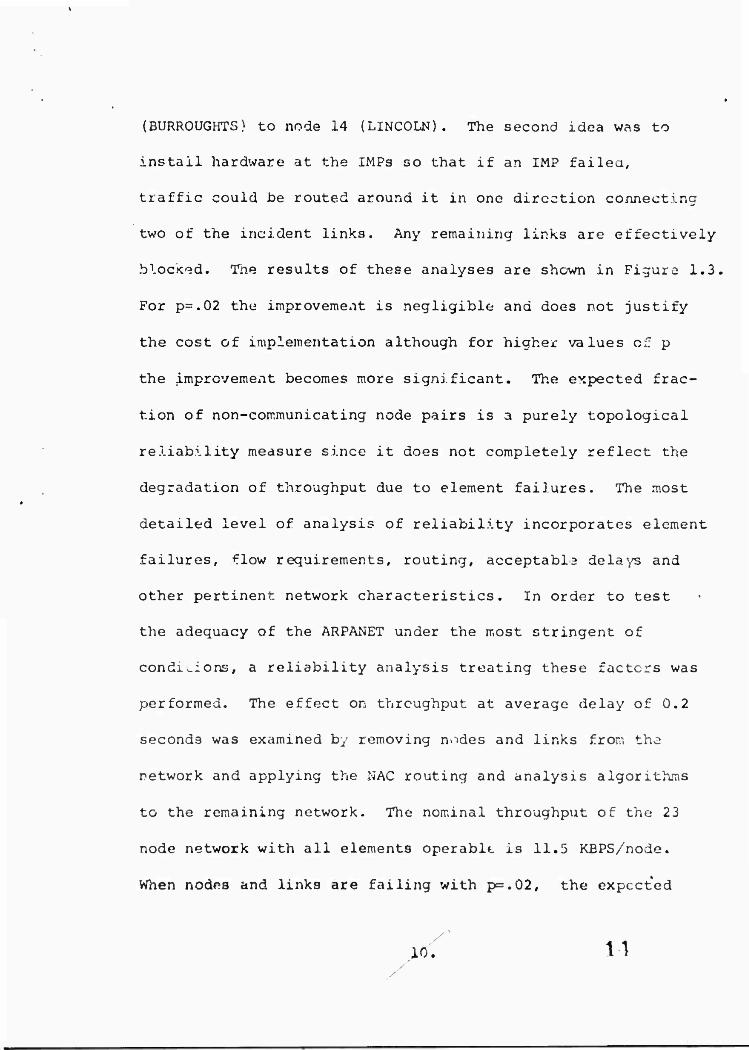
(BURROUGHTS) to node 14 (LINCOLN). The second idea was to

install hardware at the IMPs so that if an IMP failed,

traffic could be routed around it in one direction connecting

two of the incident links. Any remaining links are effectively

blocked. Tne results of these analyses are shown in Figure 1.3.

For p=.02 the improvement is negligible and does not justify

the cost of implementation although for higher values of p

the improvement becomes more significant. The expected frac-

tion of non-communicating node pairs is a purely topological

reliability measure since it does not completely reflect the

degradation of throughput due to element failures. The most

detailed level of analysis of reliability incorporates element

failures, flow requirements, routing, acceptabla delays and

other pertinent network characteristics. In order to test

the adequacy of the ARPANET under the most stringent of

conditions, a reliability analysis treating these factors was

performed. The effect on throughput at average delay of 0,2

seconds was examined by removing nvides and links from the

network and applying the NAC routing and analysis algorithms

to the remaining network. The nominal throughput of the 23

node network with all elements operable is 11.5 KEPS/node.

When nodes and links are failing with pc.02, the expected

/

10.'" 1 \

ANALYSIS OF NETWORK RELIABILITY FIGURE 1.3

Nodes and Links Failing with an

Extra Lines from BURROUGH to LINCOLN LABS

Node Failure Only

Jumpered Nodes

- Link Failures Only

Probability of Element Failing h— 1 »—^ 1 « I i

• 01 •01 03 ,04 öS .o(, ,0? 08 .09 ./

15

throughput is at least 9.0 KBPS/node. These results again

show that for small networks, reliability is not a dominant

factor.

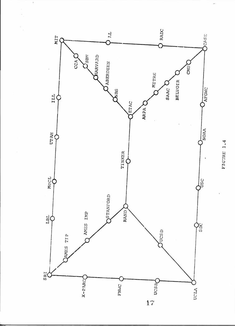
Figures 1.4 and 1.5 depict a 33 nude network. For the

network shown in Figure 1.4 the difference between the ex-

pected fraction of node pairs not communicating ~ ,058 and

2p(l-p) = .040 is almost double the difference for the 23

node network so that improving the reliability by changing

the network configuration becomes marginally feasible. An

extra link from FT.BEL to ABER increased the cost by a little

over 1% and increased the reliability by almost 10%. The

resulting network is shown xn Figure 1^5. Thus, even for a

network with only 33 nodes, it is becondng necessary to con-

sider reliability in more detail than the Mtwo connectivity" ,

criteria. For p>.02 it is even more important.

3. Reliability Trends for Large Networks

While for «Tialler networks and law element failure pro-

babilities (p6-.02), it was found that designing the network

with at least two node disjoint paths between each node pair

for throughput in the range 8-15 kilobxts/second/node guaranteed

sufficient reliability; aa networks become larger this simple

approach fails. Th3 first experiments which indicated this

1G

EH H 3

H

X) u-l

^3 o:

u D w O D M

b.

J&:

started with low cost networks of 20,40,60,80,100 and 200 nodes

with throughput approximately 8 KBPS/node designed by NAC's net-

work design program with the reliability constraint of two node

disjoint paths. The results are shown in Figure 1.6 when nodes

are perfectly reliable. TiS measured by the fraction of node

pairs not communicating, the reliability actually increased with

the number of nodes up to 60 nodes at which point the reliability

began to decrease. As is evident, the decrease in reliability is

dramatic even though nc^es have been assumed to be perfect.

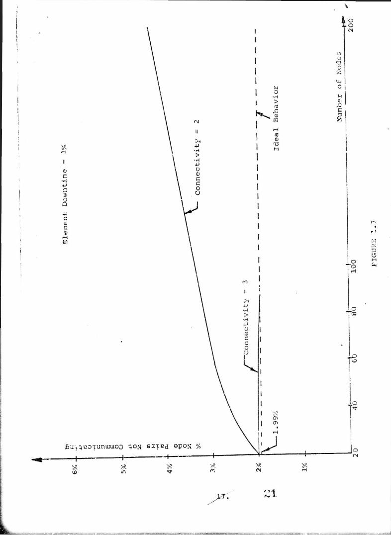
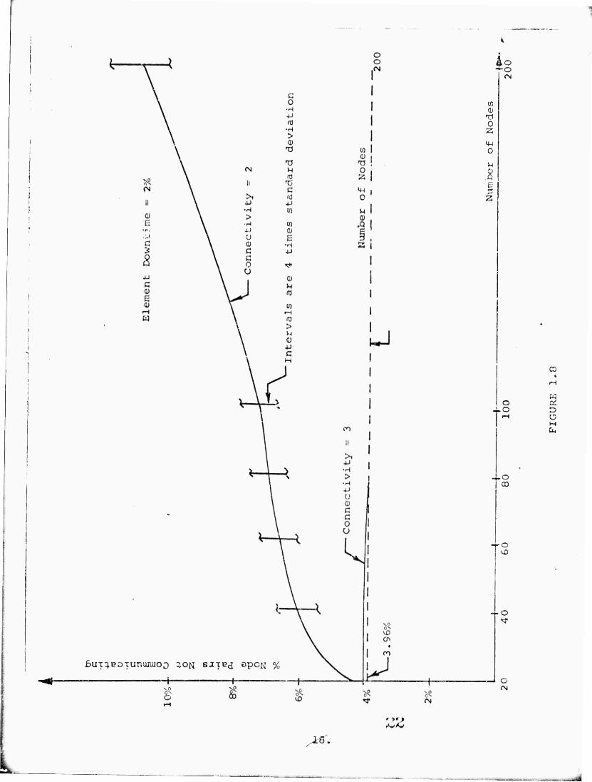
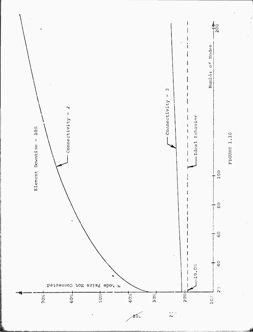
Figures 1.7 through 1.10 show the results of analysis of a

family of two and three connected networks containing from 20

nodes to 200 nodes. The networks analyzed contain 20, 40, 60,

80, 100 and 200 nodes. However, a continuous line is drawr for

visual convenience. On the curve in Figure 1.8 for p=0.2, the

simulation/analysis error is indicated by vertical bars with length

equal to 4 times the standard deviation. If the simulation results

were normally distributed, thi? would corresponde to a 95% confi-

dence interval. It can be seen from Figures 1.7 to 1.10 that when

there are 3 node disjoint paths between every pair of nodes,

the unreliability is close to the ideal minimum which results

from only the node failures within the sampling error except

for p = .1 where the 'i node disjoint paths curve is just

beginning to depart from the idea curve. From these,

19

KD

H

to

3

o

u og

D

O S3 O H

U ;.-: D

<

H

H a < H

c

w z

>1 *J •H

tj> r-i C »H

•H A Ü 03 A A

0 X u u cu 0 5 M *J rt (D W

S5 M (U CT ^ > c

0 •H 'd rH

>i (U •H -P 4J ru •H U Cu H (D •H C ^ ^5 C c 10 0 •H Ä u K-H

0 w H -H IM

0^ TJ C

CO

•H

o •a o c

o c o

•H

u

CM

J

IM

c C H

•H 4J ra o

•H C P

0 0 Ü

tM o

>1

■H

0 u 0,

0 c o o CM

g

o c

o o

c>

o c

o CO

0] Ul 00 0 0 0

■a ^ n^ c 0 0 c c c o o o KD ^ a

w c

•Ö o c o o

01 01 U)

0^3 0 oo TJ •HC CO

B ^c

o o O

ie.

^0

o L

•r;

c

s c o g

H

1 1 —H-

i o o

o 0

U-l

o u

£

O

D M

-4-° too

■tö

4°

o

in 0 ue

n ^

^yr. y,,1

m c

rn o

sz:

0

s

o o

CD

a: o 2 o D rH Ü

H fa

o CO

Bui^coiunuiuiOD ^ON SJTCCJ opOK %

■o

o

S o

,4«.

L

>1 4-1

> •H 4J U QJ C c 0 Ü

X

ßuT^BOTunuiuoo ^o^ CJTPCJ apo^ %

Csl

w o

0

o

o

E

o •H > - 0)

■ c:

re o

I I

ro g o

o •ho

o

w £ c H

-+-0 CO

o

o

'S

;.9.

rn

•H >

G c G O u

^

pa^oeuaoo ^ON SJIGJ 9po% >

fio ■fO

tn Qi

0

c

C •H >

I M

O -4- O

D

H

O CO

J1

L^

o

4- o

b UT

vC

6 o

we can conclude that requiring 3 node disjoint paths between

eveiy pair of nodes is sufficient to essentially guarantee

an optirral reliability with respect to link allocations for

networks with less than 200 nodes and for element failure

probabilities of lass than 0.1. Whether the use of this

criterion would result in expensive over-d^ ign should be

further investigated. In many cases, it is clear that this

could occur so it is worthwhile to develop rapid reliability

analysis methods which can be carried out repeatedly in the

design process. Untortunately, at present as fast as

the current reliability analysis techniques have become, it

is still infeasible to employ them in an iterative design

process.

4. Implications for Further Research

Fast effective methods have been developed for analyzing

the reliability of networks [ARPA Semi-Annual Reports 2, 3

and 4] . Recently, as wi 11 be described in the next chapter

even more efficient analysis techniques have been devebped.

Wnile these methods are effective for quite large networks,

they are still too slow for use in an iterative design

procedure. Recursive methcis suitable for networks composed

21. ^> -

■ ■

from loops and trees are orders of magnitade faster and offer

hope for use in design. These new methods are described in

the next chapter. These recursive methods can be used in a

hybrid manner with simuli»cion using decomposition techniques.

Networks which can be analyzed by recursion can also be used

as control variates in simulation of general networks.

Research is progress-'ng i~ these areas.

The selective "haraening" of important nodes in a computer

network is being studied quantitatively. It is clear that thj

only way to decrease the 2p(l-p) lower bound on the fraction

of non-communicating node pairs is to increase the reliability

of the nodes themselves. One way of doing this is to put a

backup IMP at each node. Since this is usually prohibitively

expensive, one can select a subset of nodes where backup can .

be provided on the basis of a reliability-cost tradeoff.

If-for very large networks the cost-reliability tradeoff

is the dominant factor in network design^ replacing the cost-

chroughput tradeoff, there v/ill obviously need to be dramatic

changes in network design procedures. The surface ha- been

barely broken in this area.

22.

i nnrmi ~ ^

II. RECURSIVE ANALYSIS OF NETWORK RELIABILITY

1. Introduction and Suirjnary

The network structure of many common communication networks

can be represented as a composite of simple loops and trees.

Reliability analysis of such networks can be carried out very

quickly and efficiently by a new recursion approach described

in this chapter. Moreover, a wide variety of reliability

measures can be obtained using the san«ä general method. The

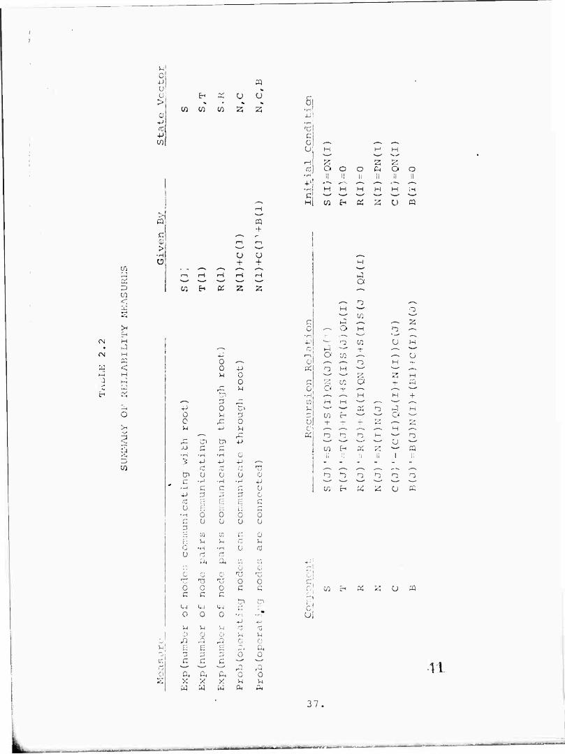
measures studied here are:

(i) the expected number of nodes communicating with a

central node called a "root",

(ii) the expected number of node pairs communicating,

(iii) the expected number of node pairs communicating by

a path through the central node,

(iv) the probability that operating nodes can communicate

through the root,

(v) the probability that operating nodes are connected.

Many other measures are possible.

In Figure 2.1 some of the many network structures that

can be analyzed using recursion are illustrated. In addition,

even if a network does not have this precise structure, the

^r. ^ i

FIGURE 2.1

COMPOSITE LOOP AND TREE STRUCTURES

(b)

''S

reliability of the network can often be approximated by the

reliability of such a network or a hybrid computation using

recursion on the tree and loop paits of the network together

with simulation for the other parts can be carried out.

(This generalized approach is now under study). These tech-

niques then offer a very powerful tool in the analysis of

network reliability.

2. Tc ninoiocrv

We will develop a very general class of recursive methods

for a wid- variety of reliability criteria. To do this it is

very economical to employ a recursive characterization of

1 rooted trees [Knuth:1968, Section 2.3] .

Definition: ä rooted tree is a finite set T of one or

more nodes such that:

(a) There is one specially viesignated node called the

root of the tree, root (T); and

(b) The remaining nodes (excluding the root) are parti-

tioned into n^ 0 disjoint sets T^, 7' , T3, ..., T . and each

of these sets in turn is a rooted tree. The trees T^# ...# T_

are called subtrees of the root.

The terminology of Knuth is somewhat different from ours.

^ w wm ■- M

As Knuth points out there are several models other than

the obvious one, a tree graph with a distinguished node, but

we will confine ourselves to tree graphs. To make this associ-

ation more explicit we introduce some more terminology. The

root of a tree, J, is said to be the father of the root of

each of the subtree- of J. The root, I, of a subtree of J

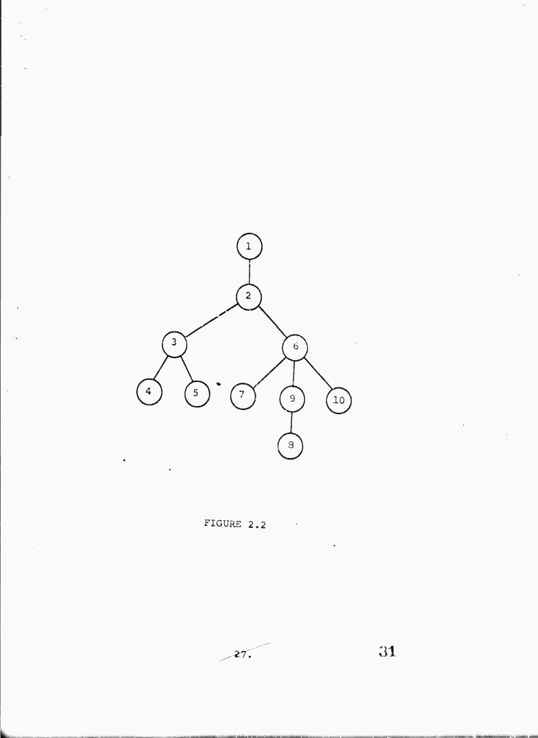
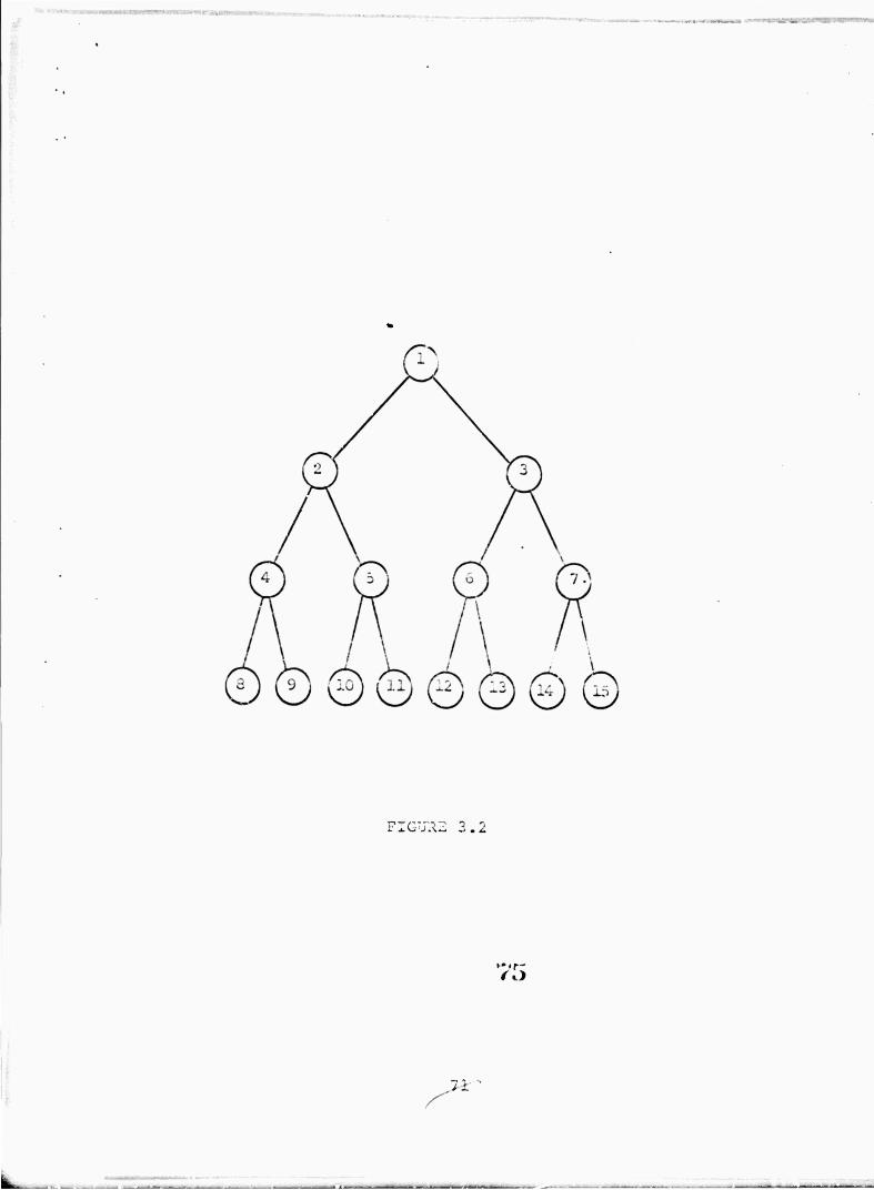
is said to be a son of J. Figure 2.2 depicts such a rooted

tree graph where links are shown between fathers and their sons.

A link is a pair of nodes one of which is the father of the

other^ Thus node 1 is the root of the entire tree. Node 2

is the root of tne only subtree of 1 and hence 2 is the son

of 1 and 1 is the father of 2. The corresponding subtree of

1 is determined by the nodes {2,3,4,5,6,7,8,9,10;. Node 2 has

two subtrees on {3,4,5| and ^6,7,8,9,10] with roots 3 and 6

respectively. Nod3 3 has two subtrees ^4^ and -15^ . Node 4

has no subtrees.

Since we will be dealing witn computer methods of solution,

it is necessary to impose a linear ordering for storage purposes,

This will be done by a father function. Suppose we have a net-

work on NN nodes, ^1,2,...,NN^, and for each node I except 1 we

have a node F(I), the father of I, such that F(I)<I and (I,F(I))

is a link in the network. Then F defines NA-NN-1 links and in

26. 30

FIGURE 2.2

,^7. 31

■ , *~- -i -

fact, the existence of a father function F is a necessary and

sufficient condition for the network to be a rooted tree. The

special node 1 (which has no father) is of course the root of

the tree (sometimes called the patriarch). Associated with

each node I is a rooted subtree consisting of nodes with

greater numbers which are connected to I by a path passing

through nodes with labels^ I. In Table 2.1 the father function

for the tree in Figure 2.2 is given.

3 * Recursive Computations on Trees

We now want to calculate the reliability of a tree network

assuming the reliability of its elements, nodes and links, are

known. It is not immediately obvious what the "reliability of

a tree" should mean; we will consider several meanings. However4

the general approach in each case will be the same. Considering

the tree to be a rooted tree in the sense of Knuth, we associate

a state vector with the root of each of the subtrees. We then

defina a set of recursion relations which yield the state vector

of a rooted tree given the state of its subtrees. For subtrees

consisting of single nodes the state is obvious. We then join

the rooted subtrees into larger and larger rooted subtrees

using the recursion relations until the state of the entire

network is obtained.

28.

mi

i

2

3

4

5

6

8

9

10

1

2

3

3

2

6

7

6

6

Father Function

TABLE 2.1

29.

33

- -"-^ ="^—^-—

Deriving the recurrence relations is somewhat mechanical

alcu. It comes simply from considering the situation depicted

in Figure 2.2. We have two subtrees one with root I and the

other having as its root J=F(I). We assume the s'cate of I and

J are known and we wish to compute the state of J relative to

the tree obtained by joining I and J by the link (I,J).

To illustrate the technique let us consider the first and

easiest criterion. Namely, we wish to know the expected number

of nodes which can carimunicate with the root node 1. We assume

we have associated with each node I a probability of r.ode failure

PNd) and a probability QN(I) = 1-PN (I) of the node being present.

Similarly, for the link (I,F(I)) we have probabilities PL(I)

and QL(I) of the link failing and being operative respectively.

The state vector of a subtree with root I is, in this case, a

scalar, S(I) which is the expected number of nodes in the sub-

tree which communicate with the root I, including I. To derive

the recurrence relatirn? we consider two subtrees with I and

J=F(I) as roots, respectively. We then want to derive the

state of the new subtree obtained by joining I and J together

by (I,J). Let S(I) and S(J) be the known states for the two

subtrees and S(J)' the resulting state. If the link (I,J)

and the node J are operational S(J)'=3(I)+S(J); if not then

30. 3-1

FIGURE 2.3

^ a:;

iin^im i «i irr'

S(J),=S(J). Putting the two together we have the recurrence

relation: S (J) ' =S (J)+S (I) QN(J) QL(I) ./here QN(J) is the proba-

bility that node J is operative and QL(I) is the probability

that the link (I#J) is operative. Now all that remains is

to put this in the form of an algorithm:

Step 0: (Initialization) Set S(I)=QN(I) (the probability

that noie I is working); 1=1,..., NN. Set I=NN. Go to Step 1.

Step 1: Let J=F(I), and set S(J) to S (J)+S (I) QN ;^ QL(I);

go to Step 2. S

Step 2: Set T to 1-1. If 1=1, stop; otherwise, go to Step 1.

When the algorithm stops S(1) is the expected number of

nodes communicating with node 1 (counting node 1).

For our next criterion we compute the expected number of

node pairs communicating. For this criterion we utilize a two

dimensional state vector. We will use, as before, S(I) to be

the expected number of nodes in the subtree which communicate

with I, and a new state component T(I) which is the expected

number of node pairs communicating in the subtree. The recur-

sion relation for S(J) is as before S(J)'=S(J)+S(I)QN(J)QL(I).

The recursion relation for T(J) is T(J)'=T(I)+T(J)+S(IjS(J)QL;l!

since we have the same pöirs communicating as before and if the

link (I,J) is operating S(I) nodes in one tree can communicate

wich S (J) nodes of the other for S{I)S(J) additional node pairs

36

The resulting algorithm is:

Step 0; (Jnitialization) Set S{I)=QN(I), T(l)=0, 1=1,..., NN.

Set I=NN. Go to Step 1.

Step 1; Let ^ F (1} ; set T(J) to T (I)+T (J)-HS (I) S (J) CL (I) , and

then set S (J) to S {J)+S (I)QN(J)QL(I). Go to Step 2.

Step 2; Set I to 1-1. If 1=1, stop; otherwise, go to Stc^ 1.

T(l) ends up with the desired result. Note in St-p 1,

T(J) must be updated before S (J).

In many real systems node pairs can communicate only through

the root. So for our next criterion, we consider the expected

number of node pairs which are connected by a path through the

root. To analyze this case we consider a state component R(I)

in place of T(I), where R(I) is the expected number of node

pairs (pairs including I are allowed) ho\.u of which are con-

nected to the root node I. S(I) has the same meaning as before.

The recurrence relation for S(I) also remains unchanged. The

recurrence relation for R(I) is R(J) ' =R(J)-f (S (I)S (J)-i-R(I) QX (J)>QL (I).

The algorithm needs only to be modified by changing the recurrence

relation for T(J) in Step 1 to the one for R(J). The state com-

ponents for this last criterion are illuminating. For if one

kn^ws the number of nodes connected to the root, say n, then

the number of node pairs communicating through the root is

*»»•« cW

33.

— -—

n(n-l)/2. This would seen to imply that either S(I) or R(I)

could be eliminated and*a state vector with one component would

be possible. This is not the case because the expectation

operation does not commute with squaring: that is, Exp[n(n-l)/2]

ft (Exp n) (Exp n -l)/2, in general, for n random.

Vie now turn to a class of reliability criteria related to

whether the network is connected or not. The first result is

immediate: the probability QC of the tree being connected is

NN NN (1) QC = TT QN(I) IT QL(I).

1 2

If we don't insist that the entire network be connected but only

the subnetwork involving operative nodes be connected we get a

new probability QC. The calculation is more interesting in this

case. Here we need a state vector for each subtree with 3

components. They are:

N(I) - The probability that all nodes in the subtree are

failed.

C(I) - The probability that the ^non-null) set of operative

nodes, including the root of the subtree, are connected.

B(I) - The probability that the root of the subtree is

failed and the set (non-null) of operative nodes in the subtree

is connected.

N(I), C(I), and B(I) account for all tree networks whose

operative nodes communicate.

an

The recurrence relations :.n this case are:

(2a} C(J),=C(I)C(J)QL(I)+C(J)N(I)

(2bj N(J) '«NCDNCJ)

(2c) B(J) ,=--B(J)N(I)+B(I)N(J)+C(T)N(J)

As we mentioned before, often in practical situations all

comnrnniration has to tzke place through the root node. So

another interesting reliability condition is the probability,

QR, that all operating nodes can communicate with the root.

As can be seen f^om the definition of C, QR=C (l)-rN(i) .

An algorithm for obtaining both criteria is;

Step 0: (Initialization) Set K(I)=PN(I), C'I)=QN(I)# 5(I)=0/

1=1, ..., NN. Set I=NN. Go to Step 1.

Step 1: Let J=F(I). Using equations (2), recalculate B(J),

C(J;, and N(J), in that order. (Note that the order of calcu-

lations is important as calculations should be done with the

old values of B(J), C(J), and N(J).) Go to Step 2.

Step 2: Set 1=1-1. If 1=1, step; otherwise, go to S^ep J..

After the algorithm terminates, we obtain the probability

of ail operating nodes communicating by CC=C(1)+B(1)TM 1) and

the probability of all operating node-, conmrnieating with the

root by QR=C(1)+N(1).

35. 39

We summarize the various algorithms in Table 2.2. The

algorithms for finding the reliability measures discussed in

this section were coded in FORTRAN IV and executed on a

CI>C-6600. The average running time for _a _5QQ node tree was

1.5 seconds.

4. Trees with W< iqhted Nodes

In the previous section it was assumed that the nodes in

the tree were all equal. In :..any cases it is desirable to

assign a weight, W(Ij# to each node, I. As an example instead

of wishing to jalculate the expected number of nodes communi-

cating with the root suppose we desired the expected amount of

traffic which could reach the root where each node, I, generates

W(I) units of traffic. To calculate this^ the state variable

is S, just as before, the only difference being that ■ehe initial

conditions S(I)- '7(J)QN(I) replaces the old initial conditions

S(I)=QN(-I). (W(I) could also represent the number of terminals

at node I.)

It is possible, by the use of a weighting function, tc

extend the algorithms of the previous section to include the

case where the "nodes" of the tree themselves represent trees,

or indeed, more highly connected graphs. In this case, m

Step 0, we initialize the state vector of'each "node" of ehe

network to the value of the state vector of the subnetwork v.'e

40

-*. -«- i -

D CO <

o. M *A

CN M QQ

W < — f-

3 t-i

c- «

o -MI u o >

>

> •H

10

EH

01 Wi

W EH

H

pq

u u m <,

& 2

u ü 4.

H

0 ^-x

0 4J u 0

c ^ ■ ^ 1 ;

^. 3 rz +> 0 tJl 0 M 3 0 ,C 0 u ^-, <4J -

^ tjl tn 4^ XJ q M

•H •H •H Ü •5 4J 4J 4J »^-N

d r- I'J T5 D> u Ü 0 a

* c .... •H •H 4J •H c c rj u *j :■ 'r~J P c^ ffl '- ::. -- .-.

t^ o C

•H 0 0 C 0 Q u u u u B £ \n w c 0 r: u u lu 5-i

0 •»H •H 0 rj

u - f3 Ä -, C-, yj

^ Ü CJ C G OJ

r-: r:. rrt --: '-' g c 0 0 0 .-, c c .: c

J7> cri U^ L, VM C : o 0 0

4J

•

j^ V4 u -- ~ ■

0 Ü Q M M ■*-■ A - - ,■'■ ' (';■

K :; •i e ■** ... . J "3 LJ 3 0 0 Ü3 C >: C -^ »«• .-; 1—^ •—- o-" Q /.

ft 0 0 2 X X :•; M u

u u^ w OH ~

5 t3 C 0 *-^ *-> —^ 0 tl H —:

1— g z z ft O c o Qi o o

•H " 11 ii II II il -P ■* - -—> .^—■* 1 -~x .—^ •i-i H H H H H H c ■,—' *-*• 1— "— —- 1—- H W &1 X z u ^

ül ex;!

CJ

X

a

— n H s-'

o w

5l

-t-

n H

Z CO o +

CO -r

CO H Ü

^

K

^ ^ 3 CO C-« ^

f-3

2

^r

O

H

u I

25

H

o a

VL

37.

are treating as aMnode.M Thus, in the previous example/we

initialize the value of S{I) to the expected nuir.ber of nodes

communicating with node I in the subnetwork we are treating

as a "node". In general it may be possible to obtain these

values analytically if the graphs are small, or it may bo

necessary to obtain them by simulation or some other means.

5• Extension 10 General Networks

In network design it is common practice to reinforce the

connections among a key set of central nodes, especially in the

case where ail communication must take place through these nodes.

An example of the simplest such configuration of this type

where the central nodes are connected in a cycle is shown

in Figure 2.4.

The algorithms we have considered can be easily extended

to handle such networks. Note first that without any modifica-

tion to the algorithms, the network shown in Figure 2.4 can be

reduced to a comparatively simple network consisting of the

central nodes only. We would consider each central node as

the root of a separate tree and analyze the tree using the

algorithms of Section 3. When the algorithm terminates, the

state vector at that node would reflect the structure of the

entire tree rooted at the node. Analysis could then be carried

30. '^

t IGURr, 2,4

39. 13

■■ iiirir¥miijMiT»TiMM"MiiTi »i ~ ■rri mmm \ ^HaHHaHMB_^H^äl^HB ■lilM^^^i i I i

out, cither analytically, or by simulation en the simplified

network of central nodes.

If the simplified network is a loop, we can use the

algorithms of Section 3 to analyze it by making the following

observation: If any component in a loop fails the resulting

network is a chain. A chain is a special kind of tree and

can be analyzed using the recursive method.

Suppose we are given a cycle w, containing N elements

(nodes and links) with ordering on the elements so that they

arc numbered e^, e0, ..., e^ in a clockwise direction starting

from some element, and that wc desire to evaluate a reliability

1 2 criterion, RL(CN)=RI^ on C^-. Consider RL^ and RLN where:

RlC=RIiv given e^ is opera tive ana

2 . . . . , , RW-RL^ given e,- is tailed.

Therefore RL^-RL^QE (N)-r-RLr?^ \^) where QE(N) is the probability

chat the element, e^, works and PE(N; is the probabili-Lv it fails,

2 , , . RL is easily evaluated by previous methods as the resulting

network is a chain. To evaluate RL.. ■ ^sider RLV nTl 1 >Tv ■ ^^s: aer i<^v„3_ ^»»^ iX,uX-]

waere:

RL,. .-ä\lA; given ^v_- is operative ana

RLr,_,"RL^ given e^.i i^ failed.

40. 11

Therefore RL^=RL^..1QE (X-1)4-RL?T-X-PE (^-D . This procedv ce

can be repeated to yield a sequence Rlj and RLJ which are

defined on disjoint segments of the total probability space and

can, therefore be suituned to yield the desired value, RLXT. A'1

of these values, with the exception of RL, can be evaluated in

terrr.s of chains and can therefore be evaluated as before. RL-,

is defined on the cycle with all components operative, and

is therefore easily evaluated. For example, if the cycle if

composed of N noaas with weights, W(I), and if RL ^s the ex-

pected number of node pairs communicating then RL-, is simply

^> t ^j W(I)W(J). Note also that the calculations of the 1=1 J^I-rl

RL- can be simplified by the observation that: two adjacent

operating elements e. and e- -, can be replaced by an equivalent

element e* with:

W(*)=QE(l)W(I)+QE(I+J)W(I+i) and

QE(*)=QE(X)QE(I+1) .

This procedure replaces the evaluation of RL on a cycle

with X evaluations of RL on chains. The order of cemputacion

is chus increased by a factor of N. The results can bo cxtondoa

still further co networks containing more than one cycle, but

the order of computation will ba increased in general by a factor

of Nc (the number of elem^ ts in the cycle) for each cycle in

41. YS

I iTl.TTl 1 Till I r»l

the network and will become excessive unless N or the number

of cycles is small.

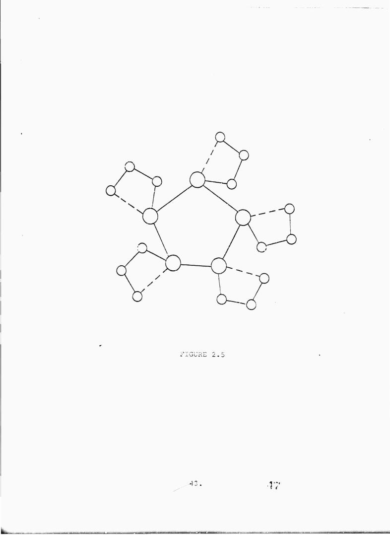
The same procedure is effective in analyzing networks of

the form shown in Figure 2.5. It can be used first en each of

the outer loops to obtain the expected number of node pairs

communicating within the given loop, 1^, and the expected

number of nodes in the loop which can communicate with e.- T .

These can then be used as initial conditions for S(I) and T(I)

in the analysis of the central loop. If there are n noces in

the inner loop and K nodes in each of the outer loops, the

2 > entire procedure can be carried out m K n+n steps.

o. Point Evaluation Versus Functional SvaTuation

The calculations in the algorithms can be carried out: in

two ways. In the first way link and node probabilities, PL(I),

QLd), PX(I}, QNiT). can be considered as numbers and the re-

liability criterion can be evaluated as a number. The evalua-

tion can also be functional; that is, the reliability of ehe

subtrees can be represented as polynomial functions of the link

and node probabilities. This approach will of course require

much more storage. The storage rcquircmerts are considerably

reduced if ail the node probabilities have the same value Pk-l-C-

as 1 all the link probabilities h..ve the same value PI^-l-QL. In

■;2.

rIUUKE 2.5

this case the various state components can ho represented by

the coefficients of power series in QN and QL.

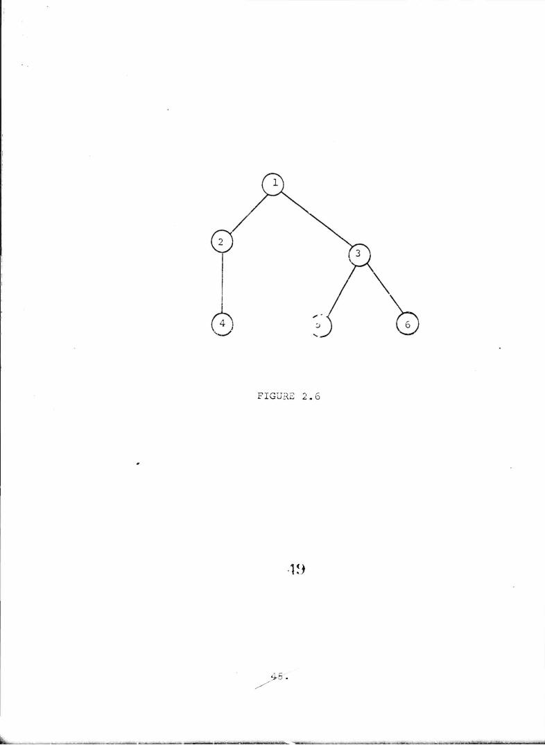
As an example we c^.rry out the calculations for the network

in Figure 2.6 using as our criterion the expected number of

node pairs communicating. We assume all links are ornative

with probability QL=p and all nodes operative with probability

CX=q.

Initialization: S(I)=q/ T(1)=0, 1=1, 2, 3, 4, 5, 6.

1^6; J^F(G)=3

T(3):=T(3)+T(6)+S(6)S(3)p

-O-rO-rqqp

2 -q p

S(3) :=S(3)+S(6)qp

=q+cqp

=q+qiip

J=F(5)=3

T(3) :=T(3)+T(5)+S{5)S(3)p

=q/1p+0-rq (q-rq p)p

=2q2p+q3p2

S(3) :=S (3)+S(5)qp

=q+q p+qqp '»^

=q+2q2p

FIGURE; 2.6

19

/*'

— —

1^4: J-F(4)=2

T(2):=T(2)+T(4)+S(4)p

2

(2) :=S (2)+s (4j

:=q-fq2P

qp

1=3: J=F(3)=1

T(l):=T(l)+T(3)+S(3)S(l)p

= (2q2p^q3p2)+(q+2q2p)qp

=jq2p+3q3p2

S(l):=S{l)+S(3)qp

-q+(q+2q2p)qp

1=2: J=F(2)=i

T{l):=T(i)+T(2)-S-(2)S(l)p

= (3q P+3qV)+qV(q+q2p) (q.-q2p+2q3p2)| 2 - 2 yj -j

=5q p+Sq^p +3q4y+2q5p4

S(l) :=S(1)+S(3)qp

I p

^^ p/qp

=q+2cÄ'p'^3q3p2

Note chat the highest order polynomia*!, qJP*% corresponds

to the longest path between two nodes (4 and 5). Xctc also

that all terras in S{1) and T^l) arc of the Jor~ q* "''p •

Thus, vc could have simplified the jalculat^ons by coi^sid

.)ü

«6.

■ -

an equivalent tree with in\ ilnerabJ links and nodes with

probability cf operation r=pq/ except for the root, which

still has probability of operation q.

:>i

47.

h^

III. A NEW ALGORITHM FOR MINIMUM SPANNING TREE CALCULATIC::

1. Intröduct2.on and Summary

A minimum spanning troe (also known as a shortest

zrec) is a troe in a networks whose total sum of link

lengths (or costs) is as small as possible. Finding a

minimum spanning tree is one of the roost common and most

important calculations in network analysis. Minimum span-

ning trees have been shown to be useful in reliability analysis

(a new application), least cost electrical wiring, minimum

cost connecting communication and transportation networks,

minimum stress networks, clustering and numerical taxonomy,

travelling salesman problems, muJtiterminal network flows,

and Telpak routing.

Currently the most favored algorithm for finding

minimum spanning trees is one due to Prim (1957] and

Di3ksLra ll9'*9j . This algorithm takes on the crd^r of n^

computations where n is the number zC nodes. It is simple

to code, conservative of computer storage and is the faseesr

rU.own method for co:.^ly- t-o n^u-vcrKs. liowovor, it i'.aj z..c

untortunatc charocteru JCIC whu.: the number of operations is

not suostanttally reuuceo v/ncn t-i'.e network is sparet,, tnat is

wr.. .. the ratio 01 links to no^^s is small as is uho «.^ase m

most practical networks such as ARPANET, Moreover, it is

too irfici-jbic for use in network reliability apol' jac^ons.

This xod KAC to re-examine an earlier solution approach

duo 4J Krushal. By judicious use of list procassing techniques

and modern sorting techniques, the computation for this method

became of the order m log m where m is the number of links.

For complete networks m = n{n-l)/2 and Prim's algorithm

is faster. However, in many applications in particular

in the reliability analysis of the AR?A network m^2n in

which case KAC's version of Kruskal's Algorithm [3ra and

4th Semi—annual reports] is much more efficient. Moreover,

NAC's version of Kruskal's algorithm is much more flexible

although at the cost of increased complexity of the algorithm.

Here we report on a dramatic improvement of Kruskal's

algorithm which makes it competative with Prim's for complete

networks also. Thus XAC's version of Prim's algorithm is

competi'tive in computation time for nearly complete networks,

is much superior for sparse networks and is mach more flexible,

The only remaining advame^e for Prim's algorithm is that in

certain situations, tne storage requirements lor neariy com-

plete networks is less for Piim's algorithm than for the

Krushal algorithm.

To be more specific we consider a network with nodes

N = 'l,...,nj and a set of m links A. Furthermore, each

4a*^ 53

link, (i#j)€.A qoing from i to ^, has a length A. . associated

wi-Ln it. We then ask what is the spanning tree of shortest

total length for N. A generalization we will also consider

is to find the shortest spanning forest with a fixed number,

k, of components.

These very simple problems in graph theory have many

practical applications. The most obvious application of

minimum length spanning trees (MSTs) is to minimum connecting

networks. Thu-, if one wanes to connect n points using the

shortest network the solution is a MST (assuming there is no

cycle or links with negative length). This fact has been

used in transportation problems, communication design problems,

and problems of wiring points together using minimum wiring

in electronic wiring problems [Loberman and Weinberger: 1957].

Kalaba [1964] considered the following type of reliability

probleifi on a network. Suppose with each link (i,j) there-

is associated a stress s,.. The oroblem is to find a minimum -^ J

stress path connecting the two given nodes; taat is, a path

connecting the two nodes such tnat the maximum stress for a

link on the chain is minimized over all chains connecting

the two given nodes. It turns our that tne path ^otwecn

two nodes determined by a MST ^s a minimum stress path.

ä0- ' 5-1

An application in which iv.iniinuin spanning forests are of

interest is in clustering anai^is under the nair.e of single

linkage cii st analysis [Gov/er and Ross: 1969] [Za.u-i; 1971].

Suppose ive ha -e a set of points, S, and a function ^(i#j)

which is a irteasure of the similarity of the points i and j.

A family of subsets i C^, of S form a o family of clusters if

for each cluster C and each pair of nodes i and j in C^ /

there is a sequence 1=1,,.,., ^v^J Wlt^ ^H'H+l^" ^ ^or

k=l#..., K-l and for every pair of nodes i and j in different

clusters /^(i,j)> I . For a given S the 5 family is unique

and corresponds co the componencs of a minimal spanning

forest over all spanning forests with he same number of

components.

A final application which motivated our interest is Monte

Carlo simulation of network reliability. Suppose we ha^e

a .etwork in which the links have a probability p of fail-

in or q^-'l-p of not failing. Wo wish -co investigate the

probability of the network "failing." The network "fails"

if it becomes disconnected. In any but the simplest cases,

exact analysis is prohibitively difficult. Monte Carlo

simulation then becomes attractive [Van Slyke and Frank: 197^]

The straightforward approach is to generate a ranacm number

r; ^ for each link (1,3)' i- ^"^ random number r. - is

greater than q the link is removed; otherwise it stays ^.n.

jtr. :i:i

. .., ,— ^* -.. ..

The resulting subnetwork is than examined to see if it is

connected. The procedure is then repeated and an estimate

is generated in the obvious way.

However, in most practical situations the probability

of the network being disconnected is desired for a range of

values for q. Suppose we want to find the probability the

network is disconnected, h(q), for all q between 0 and 1 by

Xonte Carlo simulation. A possible method is to take the

link with the smallest r• . then the link with the next

smallest r-j A and so on, until a connected graph is obtained,

Let the last link have r. . = qü. Then for q^tf the net

is disconnected for this one sample and for q i q^ the

network is connected. Thus we get one sample for every

value of q. We then generate a new set of random numbers

for the links and obtain a second sample for each value of

q and continue until the variance of the estimate is suf-

ficiently small. We then use the fraction of the times the

network was not connected as an estimate for h(q}. It turns

out that q^ can be efficiently determined by finding a

minimum spanning tree us Jig r^ ^ as the length of link (i,j).

MST's have also been applied to multiterminal network

flow analysis [Gomory and Hu: 1961] and to the solution

y oh

of traveling salesman problems [Held and Karp: 1970],

[Held and Karp: 1971].

A History of Hinirnum Spanning Tree Calculations

The first irajor contribuuion to the theory of XST's

was by Kruskal [Kruskal: 1956] plth^ugh Choquet in 1933

and^ according to Kruskal, Boruvka in 1926 did sorr.e

some earlier work. Kruskal's major contribution

was to show that a "greedy" algorithm [Edroonds: 1971]

could be used to find minimum spanning trees. Specifically,

he showed chat an MST may be obtained by repeating the

following step:

Take the shortest link which has not been

chosen or discarded. If it does not form

a cycle with some of the previously chosen

links, add it to the chosen links; other-

wise discard it.

This algorithm is deceptively simple. The means of

implementation on a computer is not obvious. The first

attempts [Obruca: 1964] were of the following form: giver*

an nxn matrix (i, ..) of link lerjths, find the smallest 11 j

entry. Do a labeling procedure to find if ehe link forms

a cyclc with rhü previously chosen link; if it does not,

save the link^otherwise discard it. In either case, make

the length of the link plus infinity and repeat the process.

Searching the matrix and examining for loops involves on the

order of n2 comparisons which must be done on the order

of n times so the running time for the algorithm in this

form is cubic in n.

Shortly thereafter P.rim [1957] and Dijkstra

[1959] proposed an algorithm which takes on the

order of n2 operations. It is ßased on the following

theorem: a tree is an KST if and only if for every ScN

there is in the tree a link of shortest length among all

those connecting a noue in S to a node in N-S [Rosenstiehl:

1967] . At every step of the algorithm we ..-ive a subset of

the nodes S and a minimum spanning tree on S. We then find

a shortest link (i/j) w^h iCS and JeN-S and add j to S

and repeat. Slightly more formally the algorithm is;

Prim's Alccrithm:

Szop 0 (Initialization) : Set S,= {XJi k^j., d1=0t S*jt d_= v(-/j)

if (l,j)€A, d-^«5 otherwise. Set fj_=0 , fjsl if (l,j)CA, a::^

f-=0 otherwise.Go to Step 1. J

Step 1 (Enlarge Sy by one node;); Let ds*=xin ^ d.: i.::.-s^; .

If d. = -v go to Stop 3; otherwise set Sv+i^S^Üjj*^ ani go

to Step 2.

Stop 2 (Update distances across cut) ; For j ^ N~^]c+i

set cL = Min|dj# 1*+ .1 and set f. = j* if dj= i-^ .-

Set k=k+l. If k=n stop. Otherwise go to Step 1.

Step 3 (Network not connected, start new component); Let j

be any node in N-S^. Set f-=0 and go to Step 2.

The total number of operations in both Step 1 and Step 2 are

quadratic in n. Moreover, since the number of links in a complete

graph, n(n-l)/2, is also quadratic in n and since in general all

links must be examined, the order of computation cannot be re-

duced to a lower order than quadratic for complete graphs.

Unfortunately, even if the graph is not complete, the order of

calculation is still quadratic since the minimization in Step 1

cannot be simplified in an easy way to take advantage of a net-

work which is spa.rse, i.e., with m/n small.

The next stage of dcterelop.Tient was to realize that if the

link lengths in Kruskal's Algorithm were presorted, efficient

sort algorithms could be utilized. Conceptually then Kruskal's

Algorithm wonld take place in two passes. First, the links are

sorted with respect to length. This takes on the order of rolo^ro

operations. Then the links are introduced in order of length

until a spanning tree is obtained^ It turns out that the order

of computation of the second pass is dominated by the computations

involved in the first pass. Thus, if the networks are sparse

and, say, the number of links, m, grows linearly with n rather

than quadratically, Kruskal's Algorithm becomes faster than Prim's;

on the other hand, for complete graphs mlog2m looks like . n ^C '—

log2 [£-^2—LL] which grows faster than the order of computation n2

required in Prim's Algorithm.

Treesort [Floyd:1962][Floyd:1964][Williams:1964] is parti-

cularly useful for use with Kruskal's Algorithm. An informal

description of Treesort along with some of its properties are

given in Appendix A. In the next section we turn to a problem

even simpler than the MST problem: namely, that of finding out

whether a network is connected or not. The solution to this

problem furnishes an efficient procedure for the second pass

in the improved Kruskal Algorithm.

3 . Finding Ccmpor.cnts of a Graph and Spanning Forests

Finding out whether an undirected graph is connected or

not in an efficient manner is not without interest in itself.

In the Monte Carlo simulation of network reliability for a single

,^. bO

value of q, for oxaiuplo, determining the connectivity of a graph

musu be carried out thousands of times so it is worthwhile to

find fast algorithms. Given the graph in node" adjacency form,

a very efficient method of determining the components is the

following:

Algorithm A:

Step ö (Initialization): Set i=l, j=l/ S=0. Label node i=l with

component label j=l.

Step 1 (Lock at new lir.k) : Find the next node i' adjacent to i;

if there are none, go to Step 3. If uode i' is not alrea in

a component, go to Step 2. If node i' ij? already labeled with

a component number, repeat Step 1.

Step 2 (Add a node to current component): Label the node i' with

the current component label j and add the index of the labeled

node to the stack S. Return wO Step 1.

Step 3 (Scan a new node): Remove a node index i" from S and set

i equal to i". Go to Step 1. If S is empty go to Step 4.

Step 4 (Current comcononu con.plotic—-start a new one); Set k

to k-t-1. If k>l, we're done; otherwise, if node k is unlabeled,

scz i to equal k and set j to j + 1. Go to S-cep 1. If node k is

labeled, repeat Step 4.

This algorithm terminates with each component having a

different label. If the links (1,1') oceurring in Step 2 arc

saved, one also obtains a spanning forest. The order of compu-

tation is linear in n and m although if the graph is nearly

complete^ the number of links m is quadratic in n. If one is

only interested in determining if the graph is connecced or not,

the algorithm can be terminated the first time Step 4 is encountered.

Tiiis algorithm is probably close to being optimally efficient if

the links are given in node adjacency form. üshakov[1967] has

proposed a similar algorithm which makes extensive use of logical

operators on vectors which for many computers would allow savings

in storage and computation time. However, he uses a node ad-

jacency representation in matrix form which requires n2 storage

locations which may largely be wasted if the graph is sparse-

Moreover, for each node ho has to search an n-vector to find

the first non-^cro eicmenu. Tnis could lead to a number of

operations en the order of nz if ^here is no special machine

instruction for rapidly carrying out th-.s operation, logically,

the two algorithms arc equivalent.

Algorithm A also has the disadvantage that the links inci-

dent to a node must all be scanned before links incident to

other nodes can be worked on. Vhis is necessary in order to

6Z ^*r.

avoid relabeling nodes. Per exar.vple, this restriction prevents

one frort adding in a simple way links to a graph already analyzed,

A slightly slower but much more flexible algorithm [Van Slyke,

and H.Frank:1972] is:

Alcorithn- E;

Step ö {Initializaticn ); 3tart with A =$ and assign each node

a separate component label. Set k=:C and go to Step 1.

Sf-ep 1 (new link): Add a link au-(ij^ j^) to Aj^ to form A^i

(if there are no remaining links; i.e., A^=A stop). Examine the

component labels of i- and j-.; if they are the same, repeat

Step 1 with k set to k-rl. If not# go to Step 2.

Step 2 (Join compenentis) ; Change all the node labels which

are the same as the label of i^ (including i^'s label) to the

label of j, . Set k to k-rl and go to Step 1.

The order of computation is dominated by the relabeling

in Step 2 which occurs n-c times where c is tho number of

components. Using a straightforward implementation [Berge:

196 2] [Berge, Ghouila - ^louri :i^65j [Scppanen :197C1

each time through Step 2.the labels on all n nodes have to be

2 checked in order to relabel. Thus, on the order of n operations

ai. "* involved with relabeling.

In the version of the algorithm used by Van Slyke ^nd Frank

[1972] a list structure was maintained so that only nodes for

63

which the labels arc changed uro considered. Further, the

number of nodes in each component was maintainod so that it was

possible to change the labels or. the smaller of the two components

joined in Step 2. This reduces the maximum order of comp^ation

to nlog2n plus a terra linear in m« This increase in speed by

using list struct v.s does incur an expense in storage requirements,

Knuth[lS68] and Read[1969] have proposed iiiaintaining component

membership using .tree data structures rather than the explicit

relabeling used in Step 2 of Algorithm B. However, in this ap-

prrach determining whether a candidate link connects two nodes

in the same or in different components takes several steps com-

pared to the one comparison required by Algorithm 3 aud is there-

fore less efficient.

4. Xcw Devc'^omonrs in MST Calculation

Until recently, the most efficienu methods for calculating

minimum spanning trees or forests was wO use Prim's algorithm

for nearly complete graphs which involves on the or^er of n^

calculation? or using ehe Xruskal Algorithm with Treescre and

AlgoritrjTi 3. The sorting p^ss takes on the order of mlog.m cal-

culations while the second pass involves nlcg^n dependence on

the number of nodes n and depones linearly on the number of links«

Thu^, for sparse graphs where mlc^1^ is small compared ^ n".

the modified Kruskal algorithm will be faster. Important con-

siderations other than speed of computation will be discussed

in Section 6; here we report on effort- to develop MST algorithms

which are uniformly fast over the full range of sparseness.

The first approach is to notice that the main expense in

the modified Kruskal Algorithm is in the sorting which takes in

general mlog^m operations and to notice that most of the links

are not considered because they make cycles with shorter links.

In Treesort (Appendix A) applied to the list of link lengths,

the list is first arranged into a binary tree which is a "heap";

that is, each link length is no longer than its descendants in

the tree . This takes about m interchanges and 2m comparisons

at the worst. Then the top link corresponding to the top of the

heap is considered via Step 1 of Algorithm B for the MST. Then

the link length is deleted from the heap and a new link length

corresponding to link (i,j), say, is taken from the bottom to

the top and the heap restored by a sift-up. The sift-up takes

at most 21og2m-l interchanges and at most 2 log2m-2 comparisons

to restore the heap. Often ehe sift-up can be saved by comparing

the component labels of i and j in Algorithm B. If they are the

same, the link forms a cycle with shorter link and can :e dis-

carded immediately. Using this approach, the sorting cost is

^ - - —

on cho order of 2m+k log0m whore k is uhe number of links cx-

aiäined in Algorithm B before a spanning tree is obtained since

only the l"nks actually considered for the KST are sorted. In

general, one may have to examine all m branches but for nearly

complete graphs this is unlikely. Experimental verification of

this is found in Section 5. There it is shown that using ^his

further modification to Xruskal's Algorithm^it becomes nearly

as efficient as Prim's Algorithm for complete graphs ^. is still

much better than Prim's Algorithm for sparse graphs.

However, Prim's method can be improved also. Mere we follow

the approach due to 2o Johnson [1972] who applied the idea« re

Dijkstra's shortosr tjath algorithm. We use Treesort -co determine

d^-Mind^ in Step 1 of Prim's Algorithm. We assume ehe d^ form

a "heap" (see Appendix A) , 'rhe top of i:he heap is d^^ which J

is then removed from the heap. Therein Step 2 of Prim's Algorithm

some of t:he d^ become smaller and are modified. Next, a d^ fi m J ' J

-he bottom of uhe heap is moved co the top. Finally, "Lhc heap

is restored. Aw the worse, each restoration of the heap takes

a numoer or operations linear in n ana usually considerably -.ess

is needed especially if the network is sparse. Even if it is

not sparse/ many of the a. dD noe change; furehermore, all bat j

one of the d. which change decrease in value so that the 3

**

__ _.__ .. B ,

'"sift-up procoduro" of Treosort tt.kcs or* a particularly simple

form (See Appendix A). In the next section we present the re-

sults of numerical .xperimenta on these clgorithms.

5 . Numerical Experir::cni:3

Numerical experiments were carried out on randomly generated

networks. For given n and m random graphs of m links and n nodes

were generated. Then a random length between 0 and I were generated

for each link. The distribution of lengths is of no importance

since as Rosenstiehl [1976] pointed out, any equivalent pre-:ordering I»

would give the same results; thus/any method which generates

random permutations of the 2inks will suffice. Three series,

four networks each, were used. These are given in 'abj.e 3.1.

Scries (n,r.l

1 m=n-l (10,9) (50,49,(100,90) (500,^99)

2 m=3n (10,3,0) v50,150} (100,300) (200,600)

3 m=n(n-l)/2 (5,10) (10,45) (20,190) (40,7£.0)

. wV^o >>. _. *\et.v/orx bones v^sea

One hundred samples of each oJ trie 12 network siiies were

an^i^yzev» ^y eacn or roar a^.gcrrtnms: Prim s »•.oa^zaca »xrasria*..

Prim s with serving, »'*carr^ad .\rus*>ial s witi p^rtia« iJO*. w. -..>

. G7

Each Cilgorith^ wao presented with exactly the seme networks,

For eacli of the algorithms e/.d each of the network sizcsy the

analysis time for each of a hundred trials was obtained. The

maximum over 100 trials, ehe averag over the 10'. trials and

ehe standard deviation over the hundi .1 trials w^s recorded.

The computer clock gives results in milliseconds and the clock

routine itself takes less than one half millisecond. The results

are presented in tabular form in Table 3.2 and in graphic-l

form in Figure 3.1. As is suggested by theory. Prim's works best

for the complete graphs ana Kruskal's works better for sparse

grapns. *ne two aj-goritrm.s using sophisticated versions ot

Treet jt yield good results ever a wide: range of sparsity. The

itoainea Krusxca^. AXcforitnni witn partia-. sorting is apoarer."Cxv

»»ne nes u ii soeec* over a wia^ rancre or soar sen ess is tr. _• cntenor

^u **Ö ^o.S 4\J 190 51.6 -tKj 780 263 . i/_.

10 9 2.29 J Ü 49 a.4, j 2 CO 99 32,28

4yy

0'/ ,72

195.33

16.07 So .^3

o. -t .

O ^ . .. '^

^ ^ v- . , C

200

▲ n m

206,22

;00, m=499 net cemputtd fcr '}.:..: -Äiiseconas en »^ v_i>s- ouwu wcm%vUtcr

/ X-

5s.o:

c e*i • » w

G8

IT' I

-'.i x^itäoconGs

200

.DU

rr.=n(n-i}/2

G€J

*&.

Milliseconds 500 -»

375^

250

125 1

rim/Sort

us y 5.1 uskal/Sort

Number of ^oces

! 125 /.DO 375 500

•k" ^^«J*V.^ «» .Kbj

TIME IN MILLISECONDS TO PIXD XST

^o

, Kr uska1/P&rtia1

FIGU.vri 3*1 (c)

IX MILX«IS£C0^3S TO FIND MST

71

MT:

6 • Sunroar^ anr; Conclusion

Speed is not the only measure in choosing an algorithm for

MST calculations. Other important considerations are: storage

requirements, form of input, availability of algorithm and diffi-

culty of implementation, the particular application, and the

number of problemo Lu be solved.

Prim's algorithm is superior in many of these respects. It

is very fasa for large nearly complete networks;- the algorithm is

easy to implement? the storage requirements are quite small es-

pecially if the network is complete and the link lengths are a

simple function of the end nodes, say Euclidean distance, • Then

the link lengths need not be stored at all but are generated once

as needed in Step 2. With the addition of Treesort in Stop 1

of the algorithir^ ^rim's Algorithm becomes much more useful for

sparse graphs; however, the algorithm becomes considerably more

complex and some speed is lost in analyzing complete graphs.

Prim's Algoriahm also has oaher disadvantages. It requires

the link information to re p/oseneed in node incidence format

and it cannot be used for determining minimum spanning forests

with various numbers of components. This latrer problem makes

Prim's Algorithm somewhat unsuitable for single lin!: .v0 cluster

analyses, rena—ixity anaiysu c J nctwor.cs, anc* muXtiLtwrminaii

network flow analysis. »-vo

The modified version of Kruskal's Algorithm is very good

for determining KST or minimum spanning forests on sparse net-

works and it accepts the links in any form. When it is used

with partial sorting, it gives the best results over the com-

plete range of sparsity. Moreover, changing to partial sorting

can be done very easily. Both versions of Kruskal's Algorithm

require a relatively large amount of storage because of the list

structures required by Algorithm 3 and in all cases require the

storage of the complete list of link lengths.

We close by analyzing two specific applications. These

are Monte Carj-O network r«--xrajr—rey an^.i-ysrs ana. single ixnkage

cluster analysis. Most practical pipelin., transportation, or

communication networks are sparse and of reasonable size. More-

over, for simluation of reliability many hundreds or thousands

of trials must be computed, Finally, if expected fraction of

node pairs communleading is u-ed as a criterion of reliability

[Van Slyke and Frank: 1972] ra-her r.han probability or being

connected, it turns oui: that minimum spanning forests are required,

Thus, the algorithm must be fast for sparse graphs, ana it :..ast

be capable of derermining minimum spanning for^sr-s. Moreover,

saoragc is usually not a problem. Th~s modified Xruskw.! is

xc*ew»<b *.or w^i^s appjLXca W^OA« •

ro

Sincj^ l^nkac;c clubtcr anaiyaitj orcscn'Co a siiCjDtiy niore

difficult cabo. Hora in general the aetwoik is complete since

cvv^ry pair of points is related, which v/ould seem to indicaca

Prim's Algorithm; however, the main rssults required arc minimum

spanning forests with various numbers of components (in order

to get the i clusters) which is not rvailable from Prim's Algorithm.

The east compromise until now was suggested by Gower and Ross [1969]

which was to do Prim's Algorithm and toss out all links not in

the KST. This leaves only n~l linKs. Then a form of Kruskal's

Algorithm is applied to find the minimum spanning forests with

various numbers of cx>mponents. This approach is still desirable

when storage is a problem and link length is a simple function

of the end nodes so that the link list need not be stored. If

there is sufficient storage, the modified Kruskal Algorithm wirh

partial sorting s^ou^e .ee mucn ^«^Swer«

■■\T5 v?-

A list of m=2;s'-l numoers n-, •••/ n-x-x can be icenwiziw«,

with a rcov.ed binarv tree with k levels where n- is at the root,

n-. ana n- are at the next icve- ana, m cenera- n->-; ana n-^-j.- at

lev^-l A-TI ari- connected to n^ at lev^l ,2, In Figure 3.2 this

iiappmc is i^.xustratea i;or x—-«.

74

«aaHMBMH

PIGuRZ 2.2

»-.f- ro

>i '

■ -

Ir={n1# ..., nj) of Icngchjc,

fJl;o list 1^ (n., ..., n5 -D'cr equivalently the binary tree

cs^ociated with it is calicä a heap if n^= n0^ and n^i n^.-.i«

The first observation is that if L is a heap then n^ß n^ for

i=l, ..., 2K-1- If for a given lis

/ / 2K-1 for scnie k, we choose the smallest k such that 2'<-l^X

and fill the unused slots with + eo. Th^ number n- is called the

father of r^^ and n^^+i and i"^ and n^j_^2. arc called the sons of

n.- . An element n^ determines a unique subtree consisting of its

sons, i.ts son's sons, and so on. In Figure 2, n^ determines the

trees ma. . up of n-, n^, n-,, nX2f ni3' ni'' ari^ ni5* ^ funda-

mental operation in Treescru is taking an element n^ for which

the subtrees determined by n.- s two sons n^-^ and n0,._^ are neaps

and by permuting elements forming a heap which is a subtree

deeermined by n^ . This is CU.11VJJ ^ sift—up of n-, although

tho way we drew Figure 3*2 ra should more properly be called a

sifw-aown. An even more .as:'c operation is an excrange-test.

at n. • rnas a«> Ctirraea Ow*^ r.i a»vv. ijueps» i'irs»«., ^o« anQ **'>-•■.*.* i £1. i.lfa

are compared; then the smaller of the two is compared with n^ .

If n- ^s larger n^ is interchanged wrtn ü ^maxier ana n^- ana

*'2i-rl*

caange•

This involves two coT.'oansons ipossioxy/ one

A sift-up of n: at level X is accomplished by pc^iorriing

an exchango-tcst at n- . If there is ur. interchange, an exchange-

rest is performed at the new position of n^ which is necessarily

aw level A^l. The procedure is continued until there is no inter-

change or until level k is reached [London: 1970]. If the subtree

determined by n^ has k levels then sift-up takes at mest k-i

exchange-tests for a total of 2k-2 comparisons and k-1 j.nterchangcs.

The first part of Treescrt consists of establishing a 'neap.

This is done recursively using sift-up. The subtrees determined

by the elements at level k-1 can be made into heaps in one ex-

change-test each; Then the elements at level k-2 are made into

heaps using sift-ups. One works up the tree until finally the

subtree determined by n, , Which is the entire tree, is made into

a heap. An element a level Ä determines a subtree with (k-JL +1)

levels hence a sift-up could take k-Jl interchanges and 2k-2A

comparisons. Since there are 2A " elements at level in the

worst case /»—.i.

A-i

interchanges and twice that many comparisons would be needw.^.

Since the length m of the list is 2 * we have what k-log^n

-nd the order of c^lculr :ion in ehe wcrce case is m-ler-, m inter-

cnanges and 2m—^ i.cg^m coxparxsons«

v: ' 77

S^nco wo havo a ho^p, the ccp ^lc::.Qnz is the sniallcSw clc-

n;cnt of ^ho list. Wc now enter ^he second phase cJ Treesort.

The to'o element is removed fro^ the heap and saved. The iasc

Jinite element of the tree is then puü at the top and sift-up

i^ earricd our until it finas irs proper level. The newest

.ecp element (uhe second smallest element of the original list)

is removed and uhe lasu fin^ce u^e:.;ent is brought to the top.

The number of interchanges in whe worse case is X-l if whe eree

has k levels regaining In general, there are 2 "^ sift-upö

carried out on X level erees. Thus there are approximately

X" (X-D 2 »2+ (}c-2)2

&

rntercn^nges ana wWice wnae ar.".oun'c or cciv.parrsons i,n üne wors^"-

for zha second oass. This Li on the order of n;log,^. If

on-.y the sr^allesu r elements ^.re recuirea rauher than a complete

ort tnen une commutation in tne secona mare as or tne oraer

£ ■*''**j p*...

.nus removed from ehe top of the heap can be suorea in re-

verse oraur in ^ne ixnuscci .i~om V-* ^- W »vj . «^_ »

l^irure j.w

elements of une

... C U *» w.. w - ■

f -

'. a \ n a tv.'O s m a -. ^. e,

* /, .. ^, *.

78

?IGU^E 3.3(a)

79 75.

^_ -■ - -

. ,_-. ^_ _

LZV£*L 1 EXCHAiCGi

80

/O.

-

HEAP

81

—■■ - -

£ -.U^i\^ J ,3 vv vÜ)

S>^L1I iST -i-.-,M^v'r ro'""^

8Ü

>^.

«4

71GCT<Z 3.3 (e)

12^1? ^ZSTG^ZD

83

f TT

-O

* XGLRä! ^ «j. {*. i

TWO SyjiLLZST ELEI'lENTS G3TAI^^D

bi

-Ä Ü .

i,-^ ^

^o a iririwii aspocc o- xrecsort wo exaniino uhc cucücio^ of

rc-esc^blishing a noap whan L.OV:^ of i*is ßlcrüents arc changed«

^"»ö -n sstablishing an initicl heap in Treci>6rt the rcmakiag of

a aaap will involve sift-ups bua aot as n\any. The elements

are sceancd starting froru the next to ehe bottom level as in

who first part of Treesort excepa ahaa a sift-up is done on an

elencnt if ana only if aha element itself is bigger than ia w^s

in the heap or if one of its sons is smaller than it originell/

was« If only decreases in value were made, as in the case in

one of the algorithms for XST's one can proceed by immediately

iwer/cing tne r—tner or aea e^eieenas aecreasea« Do a s-.-_e—up on

tne xast v—ov/e^u m neap) element mar^ced^ n. • xt tnere are any

mwCrcn^nges, mar*c tne rac*»ar o.*- n_- • KSJf.CLOfä U ne mark on n.-

W«C« '- ■rl- go to tne mar^eu e-emena lowest rn ane neap ana ccne^nue.

en regere J«** tnes procesis es j Lustrated«

85

v^e

r^

^AtfÜiVÜ ^ .-^ ^«y

86

-wu.^ J,4 (DJ

^\

PIGÜR3 4(c)

88

^t.

FIGUSS 4{<i)

89

— - - - —

•

IV, REFERENCES

1. Lobcriasui, K. and Weinberger« "PcriTial Procedures for Connecting

Terminals With a Minimum Toral Wire Lingth", JACM, 4, 42o-437#

1957.

2. Kalaba", R., "Graph Theory and Autcnatic Control", in Applied

Combinatorial Mazheiuatics, E. Beckenbach (ed.) Wiley, 1964.

3. Gower, J.C. and Ross, G.J.S., "Minimum Spanning Trees and

Single Linkage Cluster Analysis", Appl. Statistics, Vol. 13,

No. 1 54-64, 1959.

4. Zahn, C.T. "Graph-Theoretical X^chods ror Detecting and

Describing Gestalt Clusters", 7.Z:2£ Trans, on Computers, C-20,

No. 1, January, 1971.

5. Van Slyke, H. and iv-^nk, TL., "NewV/ork Reliability Analysis I",

Networks, Vol. 1, No. o, 1972.

6. Gcmory, R.E, and Hu, T.C., "Aulti-Terminal Network Flovs",

J.SIA:!, 9, No. 4, Deceniber, 1961.

7. rlcld, A. and Narp, R., ''The Travelling Salesman Problem ana

Ainimum Spanninr Trees", G:-:j:acions Research, ] S, No.6,

113£--162, Nov.-Dec. „970.

o« r*e—a, »•*. ana *sarp. A», I'n*- .*.'r;-iVc»..i.Lnc ijc«-.esrria^ Proe—em ena

1, 1971. 90

9. Xruokal, B.#Jr, "On the Shortest Spanning Subtree of a gra>h

and the Travelling Saloönian Problera1', Proc. Ar^or. Math. Soo.<

lt 43-50, 1950,

10. Chouquc:^, G,, n2wUde dc Certains Heseau de Route", C.R.Ac.Sc.,

206, 310, 1938.

11. Boruvka, "On a minimal Probien;", ?race Xoravske Pridovodeclro

Sj^odocnosti, 3, 1926.

12. ^d^ondo, J. M>iitroids and the Greedy Algorithm", ^kithomat^c^l

Programiuing, 1, No.2, 1971.

13« CiJruca, A., "AI90. 1 Xmtree" Cor^outier l>uiX2t:.m, p. 67, Sepc.

1964.

14. Prim, E.G., "Shortest Connection Ae^works and Some Generalizaticn5,r

Bell System Cjch. J., 1389-1401, i^ovemher, 1957.

15. Dijkswra, 2.W., "A Note on 2Vo Problems in Connection v;i^h Graphs",

Numarisjie r^whomg-cik, 1, 2C -11, 1959.

—o. *\Oseneuu.enl, i'., ' i-i Ar^re ^ixmmu-.T. d en Grepne* , m Theory or

^ra^hs, p. Rosenstiehl, ed., 1967, >— QOii AAAM SO, eacn f »\ • L .

17,

Aucusw 1962.

iDec»jr...>v_.., 1964.

91

19. Williaas, J.W.J., "Hoaosoro", Äigorithiu 232, ACM Collcctod

Algorithm, January, 1964.

20. Ushakov, I.A., "An Algoritl-u-i for Cnccv * the Connectivity of a

Graph", lev. AU.gcrkh.Kib., No. 4, 35-JO, 1967, Trans: Eng.

Cyb., No. 4, 32-83, 1967.

Borge, 'Thoorv of Graohs, 152-155, 1962, VTiley.

Barge, and Ghouila-Houri,A., ?roqrD::.niinq Ganges, and Transportation

Networks, 177-182, 1965, Wiley.

Seppanen, "Spanning Tree (H)u Algoritlun 399, Conu-n. ACM, 13,

No. 10, October, 1970.

Knuth, P.E., The Art of Comguter Procran:^inq; Vo^ima—Fund*

ar.3ntal Alcorith^s, Sections 2.3.3 and 2,3.4, 1968, Addiscn-

V.'esley.

25. Read, C, "Teaching Graph Theory ^o Computer", in Recena progress

m Co^bianrorics, W.T. Tutte Cod.) Academic, 1969.

26. Johnson« Personal Ccamunicaaion, 1972.

27. London, L#, "Certification of Algorithm 245 (Ml) Tree^arta'-,

C*-i'aizicataon on rw».goraann4 ^«^5, CA Co -i-actQa Alooritiinis, a^/u.

21

On

23,

24.

^1'

^Süm