82
All rights reserved © 2006, Alcatel Digitel/Alcatel – Air Interface Dimensioning 2006, February 10th Nathalie PEYROT
| Date post: | 11-Jan-2016 |
| Category: |
Documents |
| Upload: | kohlerbkqn |
| View: | 227 times |
| Download: | 9 times |

All rights reserved © 2006, Alcatel
Digitel/Alcatel – Air Interface Dimensioning
2006, February 10thNathalie PEYROT

All rights reserved © 2006, AlcatelDigitel 3G Workshop / February 2006
Derive Cell size ( <=> Cell range)
Define Site configuration Number of sectors/ antennas Number of carriers Antenna height Number of Boards
Choose Radio Feature to increase Cell capacity to improve Cell coverage
Forecast Network Evolution
Antenna 1 Antenna 2
Cell Dimensioning Purposes
To meet Operator’s targeted GoS and QoSTo meet Operator’s targeted GoS and QoS

All rights reserved © 2006, AlcatelDigitel 3G Workshop / February 2006
UTRAN dimensioning / Agenda
Challenges of UMTS Cell Dimensioning a new technology: W-CDMA Multi-Service traffic environment Coverage Capacity Trade-off
Air Interface Dimensioning

All rights reserved © 2006, AlcatelDigitel 3G Workshop / February 2006
What is going to impact Cell Dimensioning in UMTS?
1°) A New Technology: W-CDMA
Interference limitedInterference limited
Frequency reuse of 1Frequency reuse of 1
Power controlPower control
Soft HandoverSoft Handover
Cell BreathingCell Breathing

All rights reserved © 2006, AlcatelDigitel 3G Workshop / February 2006
What is going to impact Cell Dimensioning in UMTS?
2°) A Multi-service traffic environment Various Data Rates (from speech 12.2 kbps to 384 kbps)
Various QoS & GoS (Blocking, delay, throughput, BLER)
Various Connection type (Real Time (CS) or Non Real Time (PS))
Various Traffic asymmetry and behaviour
Different sensitivitiesDifferent sensitivities
Different FootprintsDifferent Footprints Speech 12.2 kbpsNRT 128 kbps
NRT 384 kbps

All rights reserved © 2006, AlcatelDigitel 3G Workshop / February 2006
Coverage and Capacity Trade-off
Multi-service Traffic
in the cell
Multi-service Traffic
in the cellCell RangeCell Range
InterferenceInterference
Need of an
iterative process
between
traffic analysis
&
link budget analysis
Need of an
iterative process
between
traffic analysis
&
link budget analysis
Understanding the network behaviour
allows a better tailored network

All rights reserved © 2006, AlcatelDigitel 3G Workshop / February 2006
Multi-service Link Budget
Multi-service Traffic ModelingMulti-service Traffic Modeling
WCDMAWCDMAMULTISERVICE Traffic MULTISERVICE Traffic
Need for a W-CDMA LKB(Cell load, Eb/N0, SHO gain…)
Different Footprints Cell breathing
Need for a Continuous coverage
Multi-service W-CDMA LKBMulti-service W-CDMA LKB

All rights reserved © 2006, AlcatelDigitel 3G Workshop / February 2006
Do we have another solution?
To avoid Complexity of traffic modelling and DL power analysis?
Rollout Phases
Phase 1 Phase 2 Phase 3 Phase 4
515
500
475
450
425
400
Feature addingFixed Cell loadReal Cell Range
Cell R
an
ge (
m)
Network Sized by Fixing Cell load to an arbitrary constant value (e.g. 50% = 3dB) in UL
Does not Reflect real Network Evolution, does not run Traffic
forecastsDoesn’t allow to set up
optimised and customised Network deployment
strategy
Coverage Holes
Therefore, Iterative Multi-service Link Budget is required

All rights reserved © 2006, AlcatelDigitel 3G Workshop / February 2006
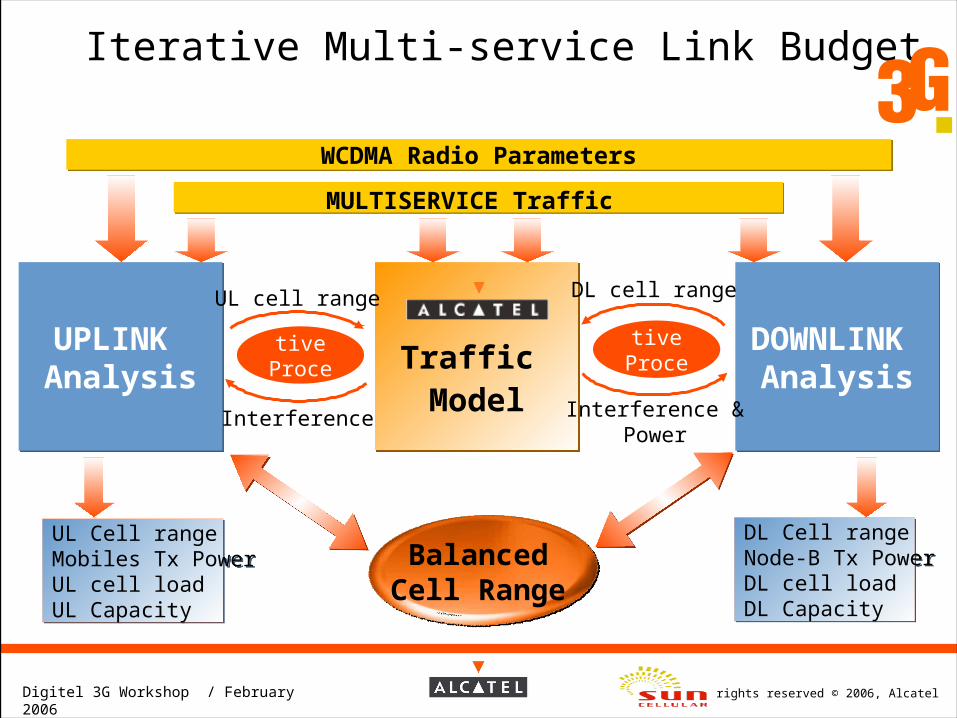
Iterative Multi-service Link Budget
WCDMA Radio ParametersWCDMA Radio Parameters
MULTISERVICE Traffic MULTISERVICE Traffic
UPLINK AnalysisUPLINK Analysis
DOWNLINK Analysis
DOWNLINK AnalysisTraffic
ModelTraffic Model
Iterative
Process
Iterative
Process
UL cell range DL cell range
Interference Interference &Power
UL Cell rangeMobiles Tx PowerUL cell loadUL Capacity
UL Cell rangeMobiles Tx PowerUL cell loadUL Capacity
DL Cell rangeNode-B Tx PowerDL cell loadDL Capacity
DL Cell rangeNode-B Tx PowerDL cell loadDL Capacity
BalancedCell Range

All rights reserved © 2006, AlcatelDigitel 3G Workshop / February 2006
UTRAN dimensioning / Agenda
Challenges of UMTS Cell Dimensioning
Air Interface Dimensioning Traffic Modelling in UMTS Uplink Analysis Downlink Analysis

All rights reserved © 2006, AlcatelDigitel 3G Workshop / February 2006
Traffic Modelling Purpose
Purpose: Dimension the different Node-B
resources in order to handle the peak of traffic and meet the GoS requirements.
Inputs Traffic Inputs provided by the Operator WCDMA Parameters Other
Means Mathematical laws Equations, Algorithms
Traffic ModelTraffic Model
Busy hour
Required Resource
Cell RangeNumber of
carriersFeatures
Number of services / SubscribersService bit rate ; Traffic volume Blocking / delay
Number of services / SubscribersService bit rate ; Traffic volume Blocking / delay
Eb/No, Chip Rate, Processing gain, Soft Handover...
Eb/No, Chip Rate, Processing gain, Soft Handover...
Traffic Model
Traffic Model
Inputs
InterferenceNode-B PowerNumber of Base Band BoardsIub interface size
C
c
c
C
block
!c
!CC,EP
0

All rights reserved © 2006, AlcatelDigitel 3G Workshop / February 2006
Traffic Modelling Example: GSM
Purpose: For considered example (GSM):
Derive the required number of TRXs
Inputs Traffic in Erlangs, Blocking rate
Means Erlang B law
E.g: One TRX with 7 traffic channels can handle 2.9 Erl @ 2% blocking
Traffic ModelTraffic Model
C
c
c
C
block
!c
!CC,EP
0
Subscriber 1
Subscriber 2
Subscriber 3
Subscriber 4
Observation Time (1H)
Call Setup
Blocked
Call Release
Peak Traffic OccurringReserved Capacity @ BTSMean Traffic Occurring
Capacity Demand

All rights reserved © 2006, AlcatelDigitel 3G Workshop / February 2006
Traffic Modelling in UMTSChallenges
Recurrent issues in UMTS dimensioning: Sharing a resource between different users How to model multi-service traffic behaviour on Air Interface How to play on different GoS requirements Derive the required capacity, but optimised
Traffic ModelTraffic Model
Average traffic
Busy hourCombination of 1 user128K +3 voice users+1 user 64K
Over-Dimensioning
OptimisedDimensioning
Under-dimensioning
Voice, SMS,
Video conferencing,
Shopping on line,
Web browsing,
File transfer,
Video games...
Aggregate traffic
All rights reserved © 2006, AlcatelDigitel 3G Workshop / February 2006
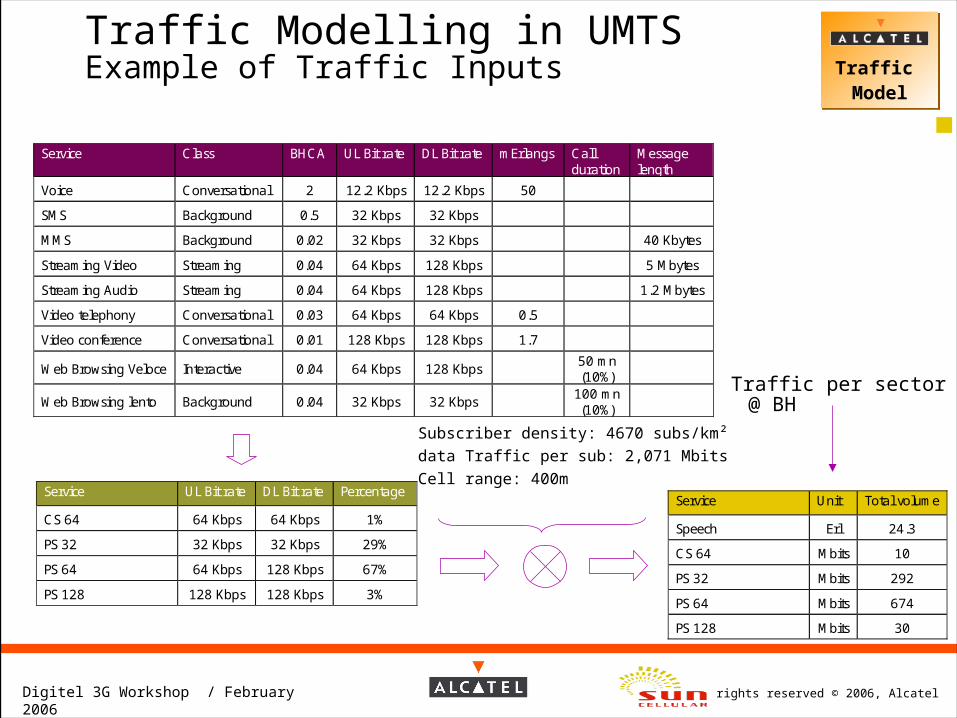
Traffic Modelling in UMTSExample of Traffic Inputs
Subscriber density: 4670 subs/km²data Traffic per sub: 2,071 MbitsCell range: 400m
Traffic ModelTraffic Model
Service Class BHCA UL Bit rate DL Bit rate mErlangs Callduration
Messagelength
Voice Conversational 2 12.2 Kbps 12.2 Kbps 50
SMS Background 0.5 32 Kbps 32 Kbps
MMS Background 0.02 32 Kbps 32 Kbps 40 Kbytes
Streaming Video Streaming 0.04 64 Kbps 128 Kbps 5 Mbytes
Streaming Audio Streaming 0.04 64 Kbps 128 Kbps 1.2 Mbytes
Video telephony Conversational 0.03 64 Kbps 64 Kbps 0.5
Video conference Conversational 0.01 128 Kbps 128 Kbps 1.7
Web Browsing Veloce Interactive 0.04 64 Kbps 128 Kbps50 mn(10%)
Web Browsing lento Background 0.04 32 Kbps 32 Kbps100 mn(10%)
Service UL Bit rate DL Bit rate Percentage
CS 64 64 Kbps 64 Kbps 1%
PS 32 32 Kbps 32 Kbps 29%
PS 64 64 Kbps 128 Kbps 67%
PS 128 128 Kbps 128 Kbps 3%
Service Unit Total volume
Speech Erl 24.3
CS 64 Mbits 10
PS 32 Mbits 292
PS 64 Mbits 674
PS 128 Mbits 30
Traffic per sector @ BH

All rights reserved © 2006, AlcatelDigitel 3G Workshop / February 2006
Traffic Modelling in UMTSWrong Approach 1: Mono-service Erlang-B Traffic
ModelTraffic Model
Service Unit Total volume
Speech Erl 24.3
CS 64 Mbits 10
PS 32 Mbits 292
PS 64 Mbits 674
PS 128 Mbits 30
Traffic per sector @ BH
Estimation of peak DL throughput (Kbps) per sector:
Results with a Mono-service Erlang-B approach:
Erlang-B applied to each service with 2% blocking
# channels
33
2
7
7
2
Multiply by each bit rate
Throughput
402.6
128
224
448
256
Total Throughput on sector:1458.6 Kbps
Wrong Approach: No resource sharing -> No spectrum Efficiency -> Over-
dimensionedBad handling of packet calls (not blocked)Does not reflect occurring traffic behaviour

All rights reserved © 2006, AlcatelDigitel 3G Workshop / February 2006
Traffic Modelling in UMTSWrong Approach 2: Average Traffic
Traffic ModelTraffic Model
Service Unit Total volume
Speech Erl 24.3
CS 64 Mbits 10
PS 32 Mbits 292
PS 64 Mbits 674
PS 128 Mbits 30
Traffic per sector @ BH
Estimation of peak DL throughput (Kbps) per sector:
Results with an Average Traffic approach:Average Throughput
148.2
2.8
81
187.2
8.3
Total Throughput on sector:427.5 Kbps
Wrong Approach: Under-dimensioned Target GoS not achieved (to much blocking)
All rights reserved © 2006, AlcatelDigitel 3G Workshop / February 2006
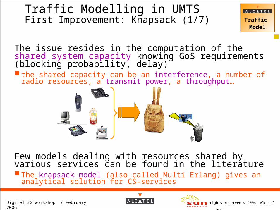
Traffic Modelling in UMTSFirst Improvement: Knapsack (1/7)
The issue resides in the computation of the shared system capacity knowing GoS requirements (blocking probability, delay) the shared capacity can be an interference, a number of radio
resources, a transmit power, a throughput…
Few models dealing with resources shared by various services can be found in the literature The knapsack model (also called Multi Erlang) gives an
analytical solution for CS-services
Traffic ModelTraffic Model
Time

All rights reserved © 2006, AlcatelDigitel 3G Workshop / February 2006
Analytical tool running Enhanced Knapsack
Traffic ModelTraffic Model
Time
Circuits services (voice and streaming)
Interactive packets services (web browsing)
Background packets services (mail)
Cap
acit
y
Busy Hour
Resource
Computation of a shared resource (by all PS and CS services): Cell load for the Uplink Power for the Downlink Throughput (Kbps)
Respects QoS and GoS
Traffic Modelling in UMTS Second Improvement: Alcatel Traffic Model

All rights reserved © 2006, AlcatelDigitel 3G Workshop / February 2006
Estimation of peak DL throughput (Kbps) per sector:
Results with a Multi-service Enhanced Knapsack approach:
Traffic Modelling in UMTS Second Improvement: Alcatel Traffic Model Traffic
ModelTraffic Model
Service Unit Total volume
Speech Erl 24.3
CS 64 Mbits 10
PS 32 Mbits 292
PS 64 Mbits 674
PS 128 Mbits 30
Traffic per sector @ BH
Total Throughput on sector:829 Kbps
Optimised Approach:Optimised dimensioning -> reflects more real traffic
occurringTarget GoS achieved for every serviceMulti-service Traffic Model for shared resource
computation
Traffic ModelTraffic Model

All rights reserved © 2006, AlcatelDigitel 3G Workshop / February 2006
Over dimensioning methods
Traffic Modelling in UMTS Comparison of the different approaches Traffic
ModelTraffic Model
Summary :
Under dimensioning method
0
200
400
600
800
1000
1200
1400
1600
Peak T
hro
ughput
(kbps)
AverageTraffic
ALCATEL Knapsackwith equalGoS for CS
and PS
Erlang-B&CSum
Erlang-Bsum
Comparison of the different traffic modelling approaches
OPTIMIZED
DIMENSIONING
All rights reserved © 2006, AlcatelDigitel 3G Workshop / February 2006
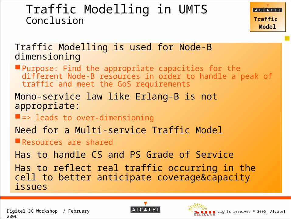
Traffic Modelling in UMTSConclusion
Traffic Modelling is used for Node-B dimensioning Purpose: Find the appropriate capacities for the different Node-
B resources in order to handle a peak of traffic and meet the GoS requirements
Mono-service law like Erlang-B is not appropriate: => leads to over-dimensioning
Need for a Multi-service Traffic Model Resources are shared
Has to handle CS and PS Grade of Service Has to reflect real traffic occurring in the cell to better anticipate coverage&capacity issues
Traffic ModelTraffic Model

All rights reserved © 2006, AlcatelDigitel 3G Workshop / February 2006
Traffic Modelling in UMTSCS Input Parameters Traffic
ModelTraffic Model
Bit rate User bit rate for the circuit connection
QoS and Radioquality
BLER and associated Eb/N0 [dB] per multipathenvironment for uplink
BLER and associated Eb/N0 [dB] per multipathenvironment for downlink
GoS Maximum acceptable Blocking Percentage
Traffic ModellingParameter
Activity Factor for uplink
Activity Factor for downlink
Number of subscribers N per sqkm and trafficintensity ‘ per subscriber (in mErlang)

All rights reserved © 2006, AlcatelDigitel 3G Workshop / February 2006
Traffic Modelling in UMTSPS Input Parameters Traffic
ModelTraffic Model
Uplink: Mean User bit rate and Peak User bit rateBit rate
Downlink: Mean User bit rate and Peak User bit rate
Uplink: BLER and associated Eb/N0 [dB] per multipath environmentQoS andRadio quality
Downlink BLER and associated Eb/N0 [dB] per multipath environment
Uplink: acceptable maximum delay time dULx% and quantile x%
(in x% of the cases, the delay has to be lower than or equal to dx%.)
GoS
Downlink acceptable maximum delay time dDLx% and quantile x%
(in x% of the cases, the delay has to be lower than or equal to dx%.)
Uplink Data Volume per busy hour V (in kbit/busy hour) per subscriber
Downlink Data Volume per busy hour V (in kbit/busy hour) per subscriber
TrafficModellingParameter
Number of subscriber N per sqkm

All rights reserved © 2006, AlcatelDigitel 3G Workshop / February 2006
UTRAN dimensioning / Agenda
Challenges of UMTS Cell Dimensioning
Air Interface Dimensioning Traffic Modelling in UMTS Uplink Analysis Downlink Analysis

All rights reserved © 2006, AlcatelDigitel 3G Workshop / February 2006
Uplink Analysis Main Characteristics
UPLINK AnalysisUPLINK Analysis
KTB
Transmit PowerP1
Transmit PowerP2
Transmit PowerP3
Transmit PowerPi
Total Interference @ Node-B
Interference Perceived by user 1
Mobiles transmit on same frequency simultaneously
Asynchronous Other UEs interfere System is interference limited
According to Power Control instructions, Mobiles adjust their power to:
Achieve target C/I Overcome Pathloss (impacted by distance) Overcome Interference (impacted by Traffic)
Interference (Iintra and Iextra) is independent of UEs’ locations

All rights reserved © 2006, AlcatelDigitel 3G Workshop / February 2006
Link Budget is performed for one mobile located at cell edge (for each service) transmitting at max power
The interference (Intra-cell and extra-cell) perceived by this UE is calculated @ Node-B, including the entire traffic mix (Traffic Model)
Interference is a shared resource
Uplink Analysis Main Concepts
UPLINK AnalysisUPLINK Analysis
cell radius
MAPL
Required Received Signal
Max UE transmit Power
UPLINK Analysis is an MAPL analysis
UPLINK Analysis is an MAPL analysis

All rights reserved © 2006, AlcatelDigitel 3G Workshop / February 2006
UL link budget elaborated for user of service k at cell edge transmitting at maximum power
cell radius
Maximum Allowable Pathloss
Reference Sensitivity
Max UE transmit Power
Gains - Losses- Margins
Interference marginintra and extra cell interference Reference
SensitivityReference Sensitivity
Transmit PowerTransmit Power
Losses and Margins
Losses and Margins
GainsGains
= MAPL
Uplink Analysis MAPL Calculation
UPLINK AnalysisUPLINK Analysis
InterferenceInterference

All rights reserved © 2006, AlcatelDigitel 3G Workshop / February 2006
Uplink Analysis MAPL Calculation / Example
UPLINK AnalysisUPLINK Analysis
W-CDMA Specific ParametersEffective Chip Rate 3840 KcpsService Bit Rate 64 KbpsProcessing Gain 17.8 dBTarget Eb/No 3.1 dBUL f ( Iintra/Iextra) 0.84
MS TransmitterTX power 21 dBm
Node-B ReceiverRX Antenna Gain 17 dBiCable and Connector losses 3 dBReceiver Noise Figure 4 dBThermal Noise -174 dBm/HzReceiver sensitivity (dBm) (to be calculated from above figures)
Gains & MarginsShadowing Margin 4.8 dBUL Rayleigh Margin 1.7 dBPenetration Margin 20 dBBody Loss 0 dB
Interference MarginInterference Margin (dB) Either fixed (e.g. 3dB) or calculated from Traffic Mix
Cell RangeMAPL (dB) (to be calculated from above figures)Cell Range (km) (to be calculated from above figures)
Example of a Mono-service UL UMTS FDD Link Budget
Service: PS 64 Kbps
Mobile Power: 21 dBm

All rights reserved © 2006, AlcatelDigitel 3G Workshop / February 2006
Rx Sensitivity calculation (for service k) : Minimum required level to reach a given quality
(C/I target) when facing only thermal noise
Where:
Nth Thermal Noise density, 10log(Nth) =-174 dBm/Hz
(Eb/N0)k : Service k target Eb/No
Rk: Service k bit rate
NF: Node-B Noise figure in dB
Reference Sensitivity = (C/I) k+NF + 10log(NthW)
and (C/I) k= (Eb/N0)k - PG
= NF +10log(Nth)+ (Eb/N0)k + 10log(Rk)
Service dependent
in dBm
in dB
Uplink Analysis MAPL Calculation / Example / Receiver Sensitivity
UPLINK AnalysisUPLINK Analysis

All rights reserved © 2006, AlcatelDigitel 3G Workshop / February 2006
Uplink Analysis MAPL Calculation / Example / Receiver sensitivity
UPLINK AnalysisUPLINK Analysis
W-CDMA Specific ParametersEffective Chip Rate 3840 KcpsService Bit Rate 64 KbpsProcessing Gain 17.8 dBTarget Eb/No 3.1 dBUL f ( Iintra/Iextra) 0.84
MS TransmitterTX power 21 dBm
Node-B ReceiverRX Antenna Gain 17 dBiCable and Connector losses 3 dBReceiver Noise Figure 4 dBThermal Noise -174 dBm/HzReceiver sensitivity (dBm) -118 dBm
Gains & MarginsShadowing Margin 4.8 dBUL Rayleigh Margin 1.7 dBPenetration Margin 20 dBBody Loss 0 dB
Interference MarginInterference Margin (dB) Either fixed (e.g. 3dB) or calculated from Traffic Mix
Cell RangeMAPL (dB) (to be calculated from above figures)Cell Range (km) (to be calculated from above figures)
Receiver Sensitivity Calculation:
Rx = 3.1 + 4 - 174 +48 Rx = -118.8 dBm
How are these margins calculated ?

All rights reserved © 2006, AlcatelDigitel 3G Workshop / February 2006
Due to Reflection and diffraction of the transmit signal on obstacle there is not only one path but a large number of paths with different delays and amplitudes
Slow fading variations due to obstacles are called shadowing
Shadowing can be modelled as a random variable with log-normal distribution of 0 mean and standard deviation that is characteristic of the environment
Uplink Analysis MAPL Calculation / Example / Shadowing Margin
UPLINK AnalysisUPLINK Analysis

All rights reserved © 2006, AlcatelDigitel 3G Workshop / February 2006
Shadowing impact on the coverage is taken into account through a “shadowing margin” in the link budget=> UE must increase their power to compensate for the shadowing anywhere in the cell
It is computed as in GSM : in a single cell
It is computed such that the average probability that this margin be exceeded in the cell is below a certain threshold => 5 to 10%
Uplink Analysis MAPL Calculation / Example / Shadowing Margin
UPLINK AnalysisUPLINK Analysis

All rights reserved © 2006, AlcatelDigitel 3G Workshop / February 2006
When a UE is at cell edge, there is a significant probability that it is in soft-handover.
Since the shadowing is partially uncorrelated between the different radio links, SHO enables to decrease the shadowing margin.
This performance gain comes from the fact that it is more unlikely to have a large attenuation for all links at the same time than for only one single link.
BS1 BS2
Same carrier
Uplink Analysis MAPL Calculation / Example / Shadowing Margin
UPLINK AnalysisUPLINK Analysis

All rights reserved © 2006, AlcatelDigitel 3G Workshop / February 2006
Depending on Shadowing standard deviation Area coverage probability Pathloss exponent K2 (Hata: K1+K2log R) Number of SHO legs
UL Shadowing margin (dB)(no SHO)
UL Shadowing margin (dB)(SHO, 2 legs)
Areacoverage
probability = 6 = 8 = 12 = 6 = 8 = 1295 % 5.9 8.7 14.6 3.1 4.8 8.5
90 % 3.3 5.4 10.0 0.6 2.1 6.4
-8
-4
0
4
8
12
16
0 5 10 15 20 25 30
Average outage probability (%)
Shadow
ing m
arg
in (dB)
Uplink Analysis MAPL Calculation / Example / Shadowing Margin
UPLINK AnalysisUPLINK Analysis

All rights reserved © 2006, AlcatelDigitel 3G Workshop / February 2006
In Uplink:Gain on shadowing marginnegligible gain on required
Eb/N0 (~0.2dB)=> slight improvement
Soft-handover gain (dB)Outage probability = 4 = 6 = 8 = 10 = 12
1 % 2.2 3.3 4.5 5.7 6.95 % 1.9 2.9 3.9 5.0 6.0
10 % 1.7 2.7 3.6 4.6 5.6
RNC
Node-BNode-B
3
3.5
4
4.5
5
5.5
6
6.5
7
7.5
8
0 5 10 15 20 25 30
Average outage probability (%)
Soft
-handover
gain
(dB
) Soft-handover gain, rho=0
Soft-handover gain, rho = 0.5
3
3.5
4
4.5
5
5.5
6
6.5
7
7.5
8
0 5 10 15 20 25 30
Average outage probability (%)
Soft
-handover
gain
(dB
) Soft-handover gain, rho=0
Soft-handover gain, rho = 0.5
Uplink Analysis Power Calculation / Example / Soft Handover
UPLINK AnalysisUPLINK Analysis
All rights reserved © 2006, AlcatelDigitel 3G Workshop / February 2006
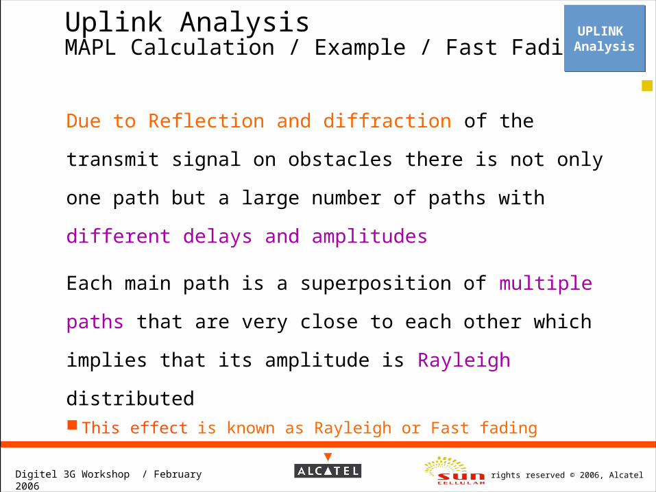
Due to Reflection and diffraction of the transmit
signal on obstacles there is not only one path but a
large number of paths with different delays and
amplitudes
Each main path is a superposition of multiple paths
that are very close to each other which implies
that its amplitude is Rayleigh distributed This effect is known as Rayleigh or Fast fading
Uplink Analysis MAPL Calculation / Example / Fast Fading
UPLINK AnalysisUPLINK Analysis

All rights reserved © 2006, AlcatelDigitel 3G Workshop / February 2006
Impact of power
control:
Fight the fading
dips
For slow-moving
mobiles, Power
control is efficient
and will
compensate the
fading-20
-15
-10
-5
0
5
10
15
20
25
0 1000 2000 3000
Slot Number (0,666 ms)
Po
wer
(d
Bm
)F
ast
fad
ing
val
ues
(d
B)
Fast fading samples (dB)
Transmit power (dBm)
0 1000 2000 3000
Slot Number (0,666 ms)
Received
P
ow
er at N
od
e-B
(d
Bm
)
Uplink Analysis MAPL Calculation / Example / Fast Fading
UPLINK AnalysisUPLINK Analysis

All rights reserved © 2006, AlcatelDigitel 3G Workshop / February 2006
When the UE is near the cell edge, it may not be able to increase its transmit power to compensate for fast fading : the transmit power is limited by the maximal UE transmit power (typically 21 or 24 dBm) Power control is not anymore efficient at cell edge : the
performance at cell edge becomes close to the one without power control
It implies a margin has to be taken into account in the link budget to compensate for the power control degradation at cell edge : this is the fast fading margin
Uplink Analysis MAPL Calculation / Example / Fast Fading
UPLINK AnalysisUPLINK Analysis

All rights reserved © 2006, AlcatelDigitel 3G Workshop / February 2006
In a single cell : difference between the required Eb/No with and without power control
However at cell edge the mobile station will be in Soft-Handoff
The UE will be power controlled by the best received cell
The selection combining of the different radio links of the active
set enables to decrease the received power variation and thus
SHO enables to decrease the fast fading margin
on PC0
b
off PC0
b
N
ERx
N
ERxg_marginFast_fadin
Uplink Analysis MAPL Calculation / Example / Fast Fading
UPLINK AnalysisUPLINK Analysis

All rights reserved © 2006, AlcatelDigitel 3G Workshop / February 2006
For medium to high speeds the For medium to high speeds the
margin margin is equal to zerois equal to zero because because
the the power control is no more efficientpower control is no more efficient
For medium to high speeds the For medium to high speeds the
margin margin is equal to zerois equal to zero because because
the the power control is no more efficientpower control is no more efficient
FAST FADING MARGIN (DB)FOR SEVERAL TARGET BLERMorpho-structure
10-1 10-2 10-3 10-4
VEHICULAR A 3KM/H
(DENSE URBAN,URBAN, SUBURBAN)
0.6 1.7 2.5 3.3
VEHICULAR A120KM/H
(RURAL)
0 0 0 0
Depending on
Channel model (Vehicular, Pedestrian)
Speed
BLER service target
0,0001
0,001
0,01
0,1
1
2 3 4 5 6 7 8
Required Eb/No (dB)
BL
ER
Without powercontrol
With powercontrol
Uplink Analysis MAPL Calculation / Example / Fast Fading
UPLINK AnalysisUPLINK Analysis

All rights reserved © 2006, AlcatelDigitel 3G Workshop / February 2006
Uplink Analysis MAPL Calculation / Example / Factor f
UPLINK AnalysisUPLINK Analysis
W-CDMA Specific ParametersEffective Chip Rate 3840 KcpsService Bit Rate 64 KbpsProcessing Gain 17.8 dBTarget Eb/No 3.1 dBUL f ( Iintra/Iextra) 0.84
MS TransmitterTX power 21 dBm
Node-B ReceiverRX Antenna Gain 17 dBiCable and Connector losses 3 dBReceiver Noise Figure 4 dBThermal Noise -174 dBm/HzReceiver sensitivity (dBm) -118 dBm
Gains & MarginsShadowing Margin 4.8 dBUL Rayleigh Margin 1.7 dBPenetration Margin 20 dBBody Loss 0 dB
Interference MarginInterference Margin (dB) Either fixed (e.g. 3dB) or calculated from Traffic Mix
Cell RangeMAPL (dB) (to be calculated from above figures)Cell Range (km) (to be calculated from above figures)
Other Important parameter:
Other Cell Interference Factor
Margins already include SHO gain
All rights reserved © 2006, AlcatelDigitel 3G Workshop / February 2006
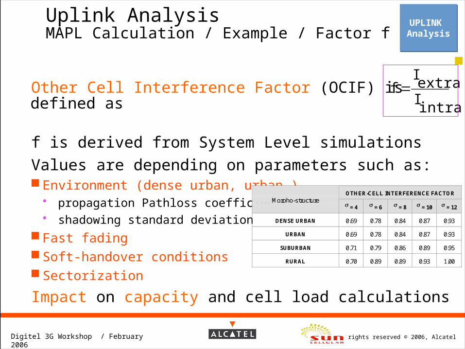
Other Cell Interference Factor (OCIF) is defined as
f is derived from System Level simulations Values are depending on parameters such as: Environment (dense urban, urban…)
propagation Pathloss coefficient shadowing standard deviation
Fast fading Soft-handover conditions Sectorization
Impact on capacity and cell load calculations
intra
Iextra
I f
Uplink Analysis MAPL Calculation / Example / Factor f
UPLINK AnalysisUPLINK Analysis
OTHER-CELL INTERFERENCE FACTORMorpho-structure
= 4 = 6 = 8 = 10 = 12
DENSE URBAN 0.69 0.78 0.84 0.87 0.93
URBAN 0.69 0.78 0.84 0.87 0.93
SUBURBAN 0.71 0.79 0.86 0.89 0.95
RURAL 0.70 0.89 0.89 0.93 1.00

All rights reserved © 2006, AlcatelDigitel 3G Workshop / February 2006
Uplink Analysis MAPL Calculation / Example / Interference
UPLINK AnalysisUPLINK Analysis
W-CDMA Specific ParametersEffective Chip Rate 3840 KcpsService Bit Rate 64 KbpsProcessing Gain 17.8 dBTarget Eb/No 3.1 dBUL f ( Iintra/Iextra) 0.84
MS TransmitterTX power 21 dBm
Node-B ReceiverRX Antenna Gain 17 dBiCable and Connector losses 3 dBReceiver Noise Figure 4 dBThermal Noise -174 dBm/HzReceiver sensitivity (dBm) -118 dBm
Gains & MarginsShadowing Margin 4.8 dBUL Rayleigh Margin 1.7 dBPenetration Margin 20 dBBody Loss 0 dB
Interference MarginInterference Margin (dB) Either fixed (e.g. 3dB) or calculated from Traffic Mix
Cell RangeMAPL (dB) (to be calculated from above figures)Cell Range (km) (to be calculated from above figures)
How to assess Interference Margin
All rights reserved © 2006, AlcatelDigitel 3G Workshop / February 2006
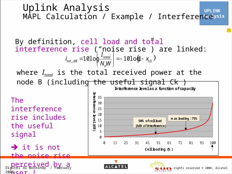
Interference level as a function of capacity
0
5
10
15
20
25
30
35
0 11 21 31 41 51 61 71 81 91 100
Cell loading (%)
50% of cell load
(3dB of interference)
max loading : 75%
Interferen
ce level (dB)
By definition, cell load and total interference rise (“noise rise”) are linked:
ULo
totaldBtot x
WN
Ii
1log10log10_
where Itotal is the total received power at the node B (including the useful signal Ck )
The interference rise includes the useful signal
it is not the noise rise perceived by a user !
UPLINK AnalysisUPLINK Analysis
Uplink Analysis MAPL Calculation / Example / Interference

All rights reserved © 2006, AlcatelDigitel 3G Workshop / February 2006
The interference rise perceived by a user of service k to be added to the MAPL calculation is then equal to :
kdBtotodB ii _
k is negligible for low data rate services, but significant for high data rate services!
UL cell load,depend on number of users in the cell
UPLINK AnalysisUPLINK Analysis
kUL
ktotal
total
o
total
o
ktotaldB
I
Clogxlog
CI
Ilog
WN
Ilog
WN
CIlogi
110110
1010100
Uplink Analysis MAPL Calculation / Example / Interference
Numerical Example
for a PS 64 user in a cell loaded at 50%:
i = 3dB - 0.14dB = 2.86 dB

All rights reserved © 2006, AlcatelDigitel 3G Workshop / February 2006
Uplink Analysis MAPL Calculation / Example / Interference
UPLINK AnalysisUPLINK Analysis
W-CDMA Specific ParametersEffective Chip Rate 3840 KcpsService Bit Rate 64 KbpsProcessing Gain 17.8 dBTarget Eb/No 3.1 dBUL f ( Iintra/Iextra) 0.84
MS TransmitterTX power 21 dBm
Node-B ReceiverRX Antenna Gain 17 dBiCable and Connector losses 3 dBReceiver Noise Figure 4 dBThermal Noise -174 dBm/HzReceiver sensitivity (dBm) -118 dBm
Gains & MarginsShadowing Margin 4.8 dBUL Rayleigh Margin 1.7 dBPenetration Margin 20 dBBody Loss 0 dB
Interference MarginInterference Margin (dB) 2.86 dB
Cell RangeMAPL (dB) 124.5 dBCell Range (km) 330 m
In Mono-service with a fixed cell load of 50%, the noise rise perceived by the considered UE:
i = 3dB - 0.14 dB = 2.86 dB
As a result:
MAPL = 124.5 dB
Cell range = 330 mMono - Service LKB

All rights reserved © 2006, AlcatelDigitel 3G Workshop / February 2006
Uplink Analysis MAPL Calculation / Example / Interference
UPLINK AnalysisUPLINK Analysis
In Multi-service:
Different Bit Rates
Different Eb/No
Different sensitivities
Different contributions to noise rise
Total interference calculated for all the subs and all services
Multi - Service LKB
W-CDMA Specific ParametersEffective Chip Rate 3840 Kcps 3840 Kcps 3840 KcpsService Bit Rate 12.2 Kbps 64 Kbps 128 KbpsProcessing Gain 25 dB 17.8 dB 14.8 dBTarget Eb/No 6.4 dB 3.1 dB 2.5 dBUL f ( Iintra/Iextra) 0.84 0.84 0.84
MS TransmitterTX power 21 dBm 21 dBm 21 dBm
Node-B ReceiverRX Antenna Gain 17 dBi 17 dBi 17 dBiCable and Connector losses 3 dB 3 dB 3 dBReceiver Noise Figure 4 dB 4 dB 4 dBThermal Noise -174 dBm/Hz -174 dBm/Hz -174 dBm/HzReceiver sensitivity (dBm) -122.7 dBm -118 dBm -116.4 dBm
Gains & MarginsShadowing Margin 4.8 dB 4.8 dB 4.8 dBUL Rayleigh Margin 1.7 dB 1.7 dB 1.7 dBPenetration Margin 20 dB 20 dB 20 dBBody Loss 3 dB 0 dB 0 dB
Interference MarginI perceived by 1 UE (dB) 2.94 dB 2.86 dB 2.75 dBTotal Interference (dB) 3 dB
Cell RangeMAPL (dB) 122 dBCell Range (km) 283 m

All rights reserved © 2006, AlcatelDigitel 3G Workshop / February 2006
UPLINK AnalysisUPLINK Analysis
Assuming perfect power control and uniform cell loading
Uplink AnalysisRelation between the number of users and the cell load
servN
jtotal
jIC
jIC
jratotaljI
C
jIC
kktotal
k
k
INIICCI
C
I
C
1int .
1..
1
raextra IfI int.
UL
erratotal
x
WN
IINI
1
. 0
intint0
servN
j jIC
jIC
jUL Nfx1 1
..1
f=OCIF factor
Note: C/I in non-logarithmic values
Multi - Service Cell Load

All rights reserved © 2006, AlcatelDigitel 3G Workshop / February 2006
Cell Load is a resource shared by all users in the cell.
Derive Peak Cell Load: Each user has a different contribution to cell load depending on its service (bit rate, QoS, CS or PS)
Uplink AnalysisPeak cell load calculation
UPLINK AnalysisUPLINK Analysis
servN
j jIC
jIC
jUL Nfx1 1
..1
Traffic ModelTraffic Model
xUL
The cell load the Cell has to be
dimensioned for

All rights reserved © 2006, AlcatelDigitel 3G Workshop / February 2006
Cell Load is a resource shared by all users in the cell.
Uplink AnalysisPeak cell load calculation / Example
UPLINK AnalysisUPLINK Analysis
servN
j jIC
jIC
jUL Nfx1 1
..1
XUL = 51.6%
(2 carriers)
Traffic per sector @ BH
Traffic ModelTraffic Model
Service C/I/(1+C/I) Total volume
Speech 0.014 24.3 Erl
CS 64 0.042 10 Mbits
PS 32 0.018 292 Mbits
PS 64 0.033 674 Mbits
PS 128 0.056 30 Mbits
KTB
Received signal 384 kbpsReceived signal 128 kbpsReceived signal Speech
Interference
Total throughput: 524 kbpsTotal throughput: 292 kbps
Received signals @ Node-B

All rights reserved © 2006, AlcatelDigitel 3G Workshop / February 2006
UPLINK AnalysisUPLINK Analysis
Assume an interference level of
I0
Assume an interference level of
I0Compute cell range through link budget
calculation
Compute cell range through link budget
calculation
Apply Traffic Model to captured traffic with this cell range :
deduce Icalc
Apply Traffic Model to captured traffic with this cell range :
deduce Icalc
Icalc = I0 ?
Icalc = I0 ?
UL RadiusUL Radius
Yes
No, adjust IoTraffic ModelTraffic Model
limiting one of all services radii
knowing nb of sub/sqkm per serviceand the QoS required per service
Uplink AnalysisMain Process

All rights reserved © 2006, AlcatelDigitel 3G Workshop / February 2006
Multi-service Link Budget is required in UMTS for Uplink Analysis
Uplink Analysis is a conventional MAPL analysis Link Budget is performed for one user of each service located at cell edge
Interference perceived by this user is generated by all the mobiles in the cell and all the services
The shared resource in Uplink is the Interference (related to cell loading)
The peak interference is calculated with a multi-service traffic model
Uplink AnalysisConclusion
UPLINK AnalysisUPLINK Analysis

All rights reserved © 2006, AlcatelDigitel 3G Workshop / February 2006
Uplink AnalysisRequired Parameters
UPLINK AnalysisUPLINK Analysis
Traffic Parameters Services, service class, bit rates, traffic volumes,
GoS Allowed blocking and delay
QoS and Radio Quality BLER and associated Eb/No, Noise Figure
Coverage Requirements Land Usage (Clutter Information), Penetration lossper clutter, Coverage Probability
Subscriber density Subs density per clutter, traffic maps
W-CDMA parameters Available frequencies, chip rate, Other CellInterference Factor, Multipath environemnt(Vehicular A3km/h, Pedestrian…)
Radio Parameters Margins (Shadowing, Fast Fading, Body-loss),Gains (antenna, SHO), Propagation Model
Site configuration Antenna height, cable losses

All rights reserved © 2006, AlcatelDigitel 3G Workshop / February 2006
UTRAN dimensioning / Agenda
Challenges of UMTS Cell Dimensioning
Air Interface Dimensioning Traffic Modelling in UMTS Uplink Analysis Downlink Analysis

All rights reserved © 2006, AlcatelDigitel 3G Workshop / February 2006
Downlink Analysis Main Characteristics
DOWNLINK Analysis
DOWNLINK Analysis
User 1
Total PowerTransmitted by Node-B
Power share dedicated to user i
User 2
User 3
User i
Node-B transmits simultaneously, on the same frequency, towards all mobiles
Power is shared by all the users, and has to satisfy all traffic in the cell
Mobiles Position and traffic will impact both: Node-B Power Interference
System is both Interference and Power limited

All rights reserved © 2006, AlcatelDigitel 3G Workshop / February 2006
DOWNLINK Analysis
DOWNLINK Analysis
Downlink Analysis Main Concepts
Link Budget is performed for all mobiles distributed in the cell (uniformly) and all services
Values of required receive signal are calculated for all positions, taking into account SHO probability, OCIF value and Pathloss
Power and Interference are shared resources determined with the traffic model
DOWNLINK Analysis is a Power analysis
DOWNLINK Analysis is a Power analysis
0,0000
0,2000
0,4000
0,6000
0,8000
1,0000
1,2000
1,4000
1,6000
1,8000
0% 20% 40% 60% 80% 100% 120%
Distance compared to the cell radius (r/R)
fact
or
f Sigma 2dB
Sigma 4dB
Sigma 6dB
sigma 8dB
0,0000
0,2000
0,4000
0,6000
0,8000
1,0000
1,2000
1,4000
1,6000
1,8000
0% 20% 40% 60% 80% 100% 120%
Distance compared to the cell radius (r/R)
fact
or
f Sigma 2dB
Sigma 4dB
Sigma 6dB
sigma 8dB
0
0.2
0.4
0.6
0.8
1
1.2
0 0.5 1 1.5 2 2.5
Probability that cell is in theactive set
Probability that cell is the onlylink
Probability of SHO and that cellis the best cell
Probability of SHO and that cellis a secondary cell
0
0.2
0.4
0.6
0.8
1
1.2
0 0.5 1 1.5 2 2.5
Probability that cell is in theactive set
Probability that cell is the onlylink
Probability of SHO and that cellis the best cell
Probability of SHO and that cellis a secondary cell
Interference
SHO

All rights reserved © 2006, AlcatelDigitel 3G Workshop / February 2006
DOWNLINK Analysis
DOWNLINK Analysis
Downlink Analysis Main Concepts
Required power calculations are performed by considering:
Mobiles suffering different path-losses (different users’ locations)
Mobiles requiring different radio quality values
(Eb/No, handover states,…)
Location dependency of factor f (ratio
between extra and intra-cell interference)
Mobiles that are not physically located
in the cell but requiring power
Power for common channels
Penetration margins and shadowing impact
Probabilistic traffic behaviour
0
0.2
0.4
0.6
0.8
1
1.2
0 0.5 1 1.5 2 2.5
Probability that cell is in theactive set
Probability that cell is the onlylink
Probability of SHO and that cellis the best cell
Probability of SHO and that cellis a secondary cell
0
0.2
0.4
0.6
0.8
1
1.2
0 0.5 1 1.5 2 2.5
Probability that cell is in theactive set
Probability that cell is the onlylink
Probability of SHO and that cellis the best cell
Probability of SHO and that cellis a secondary cell
Interference from other cells
0,0000
0,2000
0,4000
0,6000
0,8000
1,0000
1,2000
1,4000
1,6000
1,8000
0% 20% 40% 60% 80% 100% 120%
Distance compared to the cell radius (r/R)
facto
r f Sigma 2dB
Sigma 4dB
Sigma 6dB
sigma 8dB
0,0000
0,2000
0,4000
0,6000
0,8000
1,0000
1,2000
1,4000
1,6000
1,8000
0% 20% 40% 60% 80% 100% 120%
Distance compared to the cell radius (r/R)
facto
r f Sigma 2dB
Sigma 4dB
Sigma 6dB
sigma 8dB
SHO probability

All rights reserved © 2006, AlcatelDigitel 3G Workshop / February 2006
How to assess Power ?
Consider one mobile located at distance d from Node-B
Puser 1(d)dBm = Attenuation(d)dB + Itot-user 1(d)dBm + (C/I)target,dB
DOWNLINK Analysis
DOWNLINK Analysis
Downlink Analysis Power Calculation / Example
Puser
1
Itot
Cuser 1Distance d
KTB

All rights reserved © 2006, AlcatelDigitel 3G Workshop / February 2006
In Downlink NB has to compensate the channel variations for all UEs in the cell
The shadowing and Rayleigh margins are quite low (average at 2dB) since there is a very low probability that all UEs be in fading dip at the same time
One margin is taken to combine the two effects
Shadowing holesThe probability that a user at the other side of the cell faces hole of shadowing at the same time is very low
The probability that a user at the other side of the cell faces hole of shadowing at the same time is very low
A margin for each link is not realistic !
Downlink Analysis Power Calculation / Example / Shadowing Margin
DOWNLINK Analysis
DOWNLINK Analysis

All rights reserved © 2006, AlcatelDigitel 3G Workshop / February 2006
Intra-cell Interference Iintra:
User 2
Extra-cell Interference Iextra:
User 3 + User 4 User 4
Itot-user 1(d) = N0.F.W + Iintra(d) + Iextra(d)
Downlink Analysis Power Calculation / Example / Interference
Total Interference Itot-user 1(d) perceived by User 1
User 1User 2
User 3
User 4
Puser 1(d)dBm = Attenuation(d)dB + Itot-user 1(d)dBm + (C/I)target,dB
DOWNLINK Analysis
DOWNLINK Analysis

All rights reserved © 2006, AlcatelDigitel 3G Workshop / February 2006
DOWNLINK Analysis
DOWNLINK Analysis
Downlink Analysis Power Calculation / Example / Interference
Intra-cell Interference Iintra(d)
Node-B transmits simultaneously, on the same frequency, towards all mobiles
At Node-B: Transmitted signals are orthogonal thanks to the use of channelization codes
User 1
Total PowerTransmitted by Node-B
Power share dedicated to user i
User 2
User 3
User i

All rights reserved © 2006, AlcatelDigitel 3G Workshop / February 2006
DOWNLINK Analysis
DOWNLINK Analysis
Downlink Analysis Power Calculation / Example / Interference
At Mobile: Due to Multipath and reflections, orthogonality is lost
After de-spreading, some intra-cell interference remains
Reflected by the Orthogonality Factor
User 1
Total PowerTransmitted by Node-B
Power share dedicated to user i
User 2
User 3
User i
Delay 1
Intra-cell Interference
Delay 3

All rights reserved © 2006, AlcatelDigitel 3G Workshop / February 2006
The Orthogonality Factor depends on the Multipath environment (Vehicular A, Pedestrian A)
It is computed through link level simulations On-Field estimation of Orthogonality Factor is on-going
Note the lower value (higher orthogonality) in Pedestrian A due to less multi-path
Environment Orthogonality factorPedestrian 0.06Vehicular 0.4
Downlink Analysis Power Calculation / Example / Interference
DOWNLINK Analysis
DOWNLINK Analysis
All rights reserved © 2006, AlcatelDigitel 3G Workshop / February 2006
DOWNLINK Analysis
DOWNLINK Analysis
Downlink Analysis Power Calculation / Example / Interference
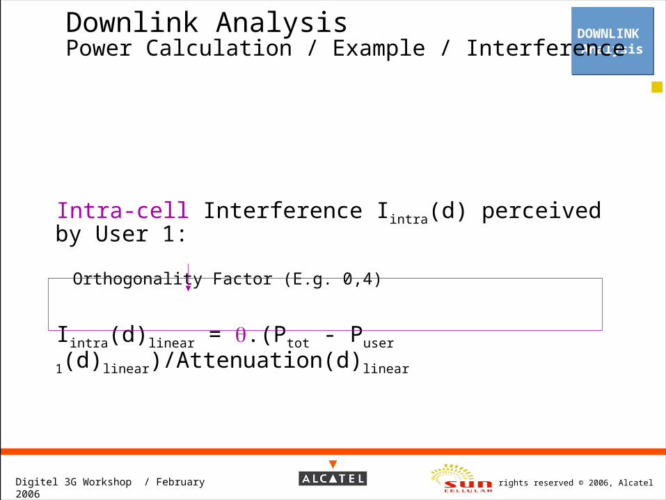
Intra-cell Interference Iintra(d) perceived by User 1:
Orthogonality Factor (E.g. 0,4)
Iintra(d)linear = .(Ptot - Puser 1(d)linear)/Attenuation(d)linear

All rights reserved © 2006, AlcatelDigitel 3G Workshop / February 2006
DOWNLINK Analysis
DOWNLINK Analysis
Downlink Analysis Power Calculation / Example / Interference
Extra-cell Interference IExtra(d)
OCIF F is location dependent in Downlink: mobiles at cell edge receives more inter-cell interference than mobiles near their serving Node-B
As for Uplink, results are derived from system level simulations
0,0000
0,2000
0,4000
0,6000
0,8000
1,0000
1,2000
1,4000
1,6000
1,8000
0% 20% 40% 60% 80% 100% 120%
Distance compared to the cell radius (r/R)
fact
or
f Sigma 2dB
Sigma 4dB
Sigma 6dB
sigma 8dB

All rights reserved © 2006, AlcatelDigitel 3G Workshop / February 2006
DOWNLINK Analysis
DOWNLINK Analysis
Downlink Analysis Power Calculation / Example / Interference
Extra-cell Interference Iextra(d) perceived by User 1:
Other Cell Interference Factor (for Downlink)
IExtra(d)linear = F(d).Ptot/Attenuation(d)linear

All rights reserved © 2006, AlcatelDigitel 3G Workshop / February 2006
DOWNLINK Analysis
DOWNLINK Analysis
Downlink Analysis Power Calculation / Example / Interference
So, Total Interference Itot-user 1(d) perceived by User 1
Itot-user 1(d) = N0.F.W + Iintra(d) + Iextra(d)
Itot-user 1(d) = N0.F.W + [.(Ptot - Puser 1(d)) + F(d).Ptot ]/Attenuation(d)
And Total Interference Itot(d)
Itot(d) = N0.F.W + [( + F(d)).Ptot ]/Attenuation(d)
Example, with: Node-B transmitting @ 43 dBm, attenuation of 129 dB, =0.4, F(d)=0.6 Itot(d)dBm = - 86 dBm

All rights reserved © 2006, AlcatelDigitel 3G Workshop / February 2006
Finally, the expression of Puser 1(d) can be put under the form
Puser 1(d) = auser 1(d).Ptot+ buser 1(d)
Where,
auser 1(d) = (C/I)target/(1+(C/I)target).( + F(d))
buser 1(d) = (C/I)target/(1+(C/I)target)[N0.F.W.Attenuation(d)
Comments: One term to compensate for Interference (traffic) and one term to compensate for Propagation and Thermal Noise
Downlink Analysis Power Calculation / Example / Power
(C/I)target=(Eb/No) target /PG/SHO_gain
For user in SHO status
Puser 1(d)dBm = Attenuation(d)dB + Itot-user 1(d)dBm + (C/I)target,dB
DOWNLINK Analysis
DOWNLINK Analysis

All rights reserved © 2006, AlcatelDigitel 3G Workshop / February 2006
In Uplink:Gain on shadowing marginnegligible gain on required
Eb/N0 (~0.2dB)=> slight improvement
In Downlink: Gain on Eb/N0 : reduce the
Eb/No target of ~2.5dB (according to simulations)
Soft-handover gain (dB)Outage probability = 4 = 6 = 8 = 10 = 12
1 % 2.2 3.3 4.5 5.7 6.95 % 1.9 2.9 3.9 5.0 6.0
10 % 1.7 2.7 3.6 4.6 5.6
RNC
Node-BNode-B
3
3.5
4
4.5
5
5.5
6
6.5
7
7.5
8
0 5 10 15 20 25 30
Average outage probability (%)Soft
-handover
gain
(dB
) Soft-handover gain, rho=0
Soft-handover gain, rho = 0.5
3
3.5
4
4.5
5
5.5
6
6.5
7
7.5
8
0 5 10 15 20 25 30
Average outage probability (%)Soft
-handover
gain
(dB
) Soft-handover gain, rho=0
Soft-handover gain, rho = 0.5
Downlink Analysis Power Calculation / Example / Soft Handover
DOWNLINK Analysis
DOWNLINK Analysis

All rights reserved © 2006, AlcatelDigitel 3G Workshop / February 2006
DOWNLINK Analysis
DOWNLINK Analysis
Downlink Analysis Power Calculation / Example / Soft Handover
The required power depends on the Handover status of the UE:
Mobile linked to the Node-B, not in SHO
Mobile linked to the Node-B as best cell, in SHO
Mobile linked to the Node-B in secondary cell, in SHO
0
0.2
0.4
0.6
0.8
1
1.2
0 0.5 1 1.5 2 2.5
Probability that cell is in theactive set
Probability that cell is the onlylink
Probability of SHO and that cellis the best cell
Probability of SHO and that cellis a secondary cell

All rights reserved © 2006, AlcatelDigitel 3G Workshop / February 2006
Impact of User Position on Capacity
DL power is shared !
Node B Cell edge
0
Nu
mb
er
of
Users
50 100
DL Capacity = Function (UE distribution)
% Cell Range
Downlink Analysis Power Calculation / Example / Power
DOWNLINK Analysis
DOWNLINK Analysis
Node-B power of 20W, 4W being allocated to Common Channels and 2 dB for shadowing
Users at 50% Cell Range: With 1006 mW per user, 9 PS 64 users can be supported Users at Cell Edge: With 1842 mW per user, only 5 PS 64 users can be supported
10 W

All rights reserved © 2006, AlcatelDigitel 3G Workshop / February 2006
Three main solutions to compute the DL power
All users @ cell edgeAll users @ cell edge solution very pessimistic low capacity
All users @ cell edgeAll users @ cell edge solution very pessimistic low capacity
30% of mobiles @ cell edge and 30% of mobiles @ cell edge and 70% of UE @mid cell range70% of UE @mid cell range
Does not reflect the statistical behaviour of the cell and may lead to an under-dimensioninglow accuracy on capacity computation
30% of mobiles @ cell edge and 30% of mobiles @ cell edge and 70% of UE @mid cell range70% of UE @mid cell range
Does not reflect the statistical behaviour of the cell and may lead to an under-dimensioninglow accuracy on capacity computation
Uniform user distributionUniform user distribution solution more realistic higher accuracy on capacity computation
Uniform user distributionUniform user distribution solution more realistic higher accuracy on capacity computation
Downlink Analysis Power Calculation / Example / Power
DOWNLINK Analysis
DOWNLINK Analysis
Cell Range
DL power is shared !

All rights reserved © 2006, AlcatelDigitel 3G Workshop / February 2006
Deriving a mean power per user for one specific service, no more dependent from location, thanks to a uniform user distribution WITH associated probability of Handover status and OCIF
We have the required power at distance d:
Puser i(d) = auser i(d).Ptot+ buser i(d)
to get the mean Power:
Example of mean power: 29.2 dBm 12 supported users at 64 Kbps
DOWNLINK Analysis
DOWNLINK Analysis
Downlink Analysis Power Calculation / Total Power
i user , mean i user , mean i user tot i userR
i user , meanb Ptot . a dr )r( b P )r( a P 20

All rights reserved © 2006, AlcatelDigitel 3G Workshop / February 2006
DOWNLINK Analysis
DOWNLINK Analysis
Downlink Analysis Power Calculation
The total required Node-B power equation can be expressed, in Multi-service:
m.aj.N
bj.NPPP
P
jservicesalloverj
jservicesalloverjCCHotherSCHCPICH
tot
1
Shadowing effect
Parameter Default value Range
P-CPICH power33 dBm (-10dB compared to
the Node B max power)-10 dBm to 43 dBm
P-SCH power - 5dB -15 dB to 35 dBS-SCH power - 5dB -15 dB to 35 dBBCH power (P-CCPCH) - 2 dB -15 dB to 35 dBFACH power (S-CCPCH) - 2 dB -15 dB to 35 dBPCH power (S-CCPCH) - 2 dB -15 dB to 35 dBPICH power - 5 dB -15 dB to 35 dBAICH power - 9 dB -15 dB to 35 dB
4 W are typically considered for
Common Control Channels

All rights reserved © 2006, AlcatelDigitel 3G Workshop / February 2006
The power equation can be expressed in the following form:
The terms YDL and XDL are derived thanks to the traffic module
Downlink Analysis Power Calculation
DOWNLINK Analysis
DOWNLINK Analysis
)traffic(x
)R,traffic(yP
DL
1
Traffic ModelTraffic Model
XDL & YDL
All rights reserved © 2006, AlcatelDigitel 3G Workshop / February 2006
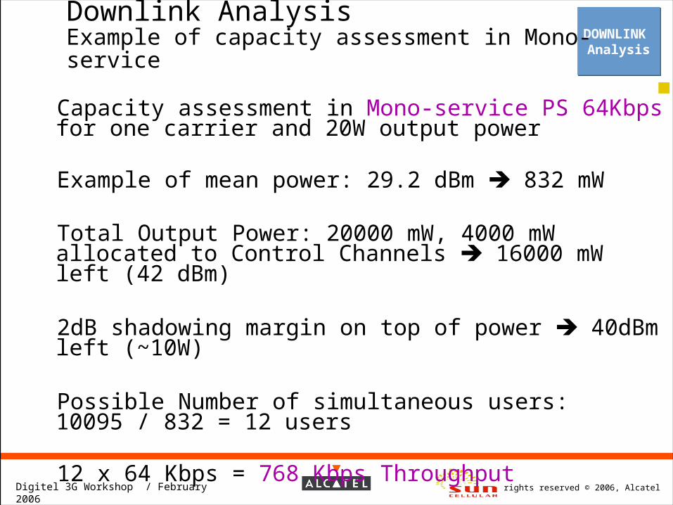
Capacity assessment in Mono-service PS 64Kbps for one carrier and 20W output power
Example of mean power: 29.2 dBm 832 mW
Total Output Power: 20000 mW, 4000 mW allocated to Control Channels 16000 mW left (42 dBm)
2dB shadowing margin on top of power 40dBm left (~10W)
Possible Number of simultaneous users: 10095 / 832 = 12 users
12 x 64 Kbps = 768 Kbps Throughput
DOWNLINK Analysis
DOWNLINK Analysis
Downlink Analysis Example of capacity assessment in Mono-service

All rights reserved © 2006, AlcatelDigitel 3G Workshop / February 2006
Downlink Analysis Main Process
DOWNLINK Analysis
DOWNLINK Analysis
Assume a cell range Ro
Assume a cell range Ro
Apply Traffic Model to captured traffic and compute total DL
Power for traffic channels
Apply Traffic Model to captured traffic and compute total DL
Power for traffic channels
Compute total DL power Ptot by adding power for common
channels
Compute total DL power Ptot by adding power for common
channels
Ptot = Pmax
?Ptot = Pmax
?
DL RadiusDL Radius
Yes
No, adjust Ro
Traffic ModelTraffic Model
knowing nb of sub/sqkm per service and the QoS required per service

All rights reserved © 2006, AlcatelDigitel 3G Workshop / February 2006
Key dimensioning radio parametersCritical parameters
Critical parameters that strongly affect the design results: penetration margin (from 0 to 22dB)
Offered service (from 128kbps to 384kbps, double the number of sites)
Propagation model parameters (morpho correction factor Kc)
Probability of coverage (90, 95%)
Mobile transmit power (21 or 24 dBm)
Max allowable UL cell load (e.g. 65%)
EB/No (e.g. 6.4 dB in Uplink)
Multipath channel model (Vehicular or Pedestrian) and speed (3-120km/h)

All rights reserved © 2006, AlcatelDigitel 3G Workshop / February 2006
Downlink analysis is not a conventional link budget but a power analysis
This Power analysis is performed for all users of all services in the cell.
User’s Position has a great impact on capacity The shared resources in Downlink are the Power and the Interference
The peak Power is calculated with a Multi-service traffic model
Downlink AnalysisConclusion
DOWNLINK Analysis
DOWNLINK Analysis

All rights reserved © 2006, AlcatelDigitel 3G Workshop / February 2006
Downlink AnalysisRequired Parameters
Traffic Parameters Services, service class, bit rates, traffic volumes,
GoS Allowed blocking and delay
QoS and Radio Quality BLER and associated Eb/No, Noise Figure
Coverage Requirements Land Usage (Clutter Information), Penetration lossper clutter, Coverage Probability
Subscriber density Subs density per clutter, traffic maps
W-CDMA parameters Available frequencies, chip rate, Other CellInterference Factor, Multipath environement(Vehicular A3km/h, Pedestrian…), OrthogonalityFactor
Radio Parameters Margins (Shadowing, Fast Fading, Body-loss),Gains (antenna, SHO), Propagation Model
Site configuration Antenna height, cable losses
DOWNLINK Analysis
DOWNLINK Analysis
All rights reserved © 2006, AlcatelDigitel 3G Workshop / February 2006
Iterative Multi-service Link Budget
WCDMA Radio ParametersWCDMA Radio Parameters
MULTISERVICE Traffic MULTISERVICE Traffic
UPLINK AnalysisUPLINK Analysis
DOWNLINK Analysis
DOWNLINK AnalysisTraffic
ModelTraffic Model
Iterative
Process
Iterative
Process
UL cell range DL cell range
Interference Interference &Power
UL Cell rangeMobiles Tx PowerUL cell loadUL Capacity
UL Cell rangeMobiles Tx PowerUL cell loadUL Capacity
DL Cell rangeNode-B Tx PowerDL cell loadDL Capacity
DL Cell rangeNode-B Tx PowerDL cell loadDL Capacity
BalancedCell Range

www.alcatel.com


