05-11 Working Paper - University of Sydney Business...

I T L S

INSTITUTE of TRANSPORT and LOGISTICS STUDIES The Australian Key Centre in Transport and Logistics Management

The University of Sydney Established under the Australian Research Council’s Key Centre Program.

WORKING PAPER ITLS-WP-05-11 Designing a Procedure to Undertake Long Term Evaluation of the Effects of TravelSmart Interventions By Peter Stopher, Stephen Greaves, Min Xu* & Natalie Lauer *NSW Dept of Infrastructure Planning & Natural Resources Sydney NSW Australia June 2005 ISSN 1832-570X

NUMBER: Working Paper ITLS-WP-05-11 TITLE: Designing a Procedure to Undertake Long Term

Evaluation of the Effects of TravelSmart Interventions ABSTRACT: As part of the program of strategies to reduce the emission of

greenhouse gases in Australia, the ACT, Queensland, South Australian, and Victorian governments have joined together to undertake a program of voluntary travel behaviour change (VTBC) strategies. This paper outlines and evaluates the options available for a long term monitoring program to measure the effects of VBTC interventions. In particular, it deals with which measurement method to employ, how to conduct the sampling, how frequently to measure the population, and how to enhance the primary data set for a national monitoring program. The paper explores a wide range of options available to the project partners. At a minimum, it is recommended that a purpose-specific annual odometer survey be conducted on a rotating panel of households. However, a far richer data set would be provided through the use of personal global positioning systems (GPS) devices for data collection over periods of up to 1 month at six-monthly intervals on a panel of households. A number of combinations of these two survey methods are suggested. The paper considers the use of established tools, such as travel diaries, and established surveys, such as the SMVU, but ultimately finds them inadequate for the task. In recommending pioneering new monitoring methods and practices, the authors acknowledge a number of areas which will require further investigation. Specifically, further investigation of issues relating to respondent burden and data variability in different survey designs will need to be conducted. Much work will be required to develop and test the instruments to be employed in the administration of the options recommended in this paper.

KEY WORDS: Evaluation, travel behaviour change, panels AUTHOR/S: Peter Stopher, Stephen Greaves, Min Xu* & Natalie Lauer CONTACT: Institute of Transport and Logistics Studies (C37) An Australian Key Centre

The University of Sydney NSW 2006 Australia Telephone: +61 9351 0071 Facsimile: +61 9351 0088 E-mail: [email protected] Internet: http://www.itls.usyd.edu.au DATE: June 2005

Designing a Procedure to undertake long term evaluations of the effects of TravelSmart intervention

Stopher, Greaves, Xu & Lauer

1

1. The Issues

As part of the program of strategies to reduce the emission of greenhouse gases in Australia, the ACT, Queensland, South Australia, and Victoria have joined together to undertake a program of voluntary travel behaviour change (VTBC) strategies1. Based on implementation of such strategies in a few locations around Australia, estimates have been made of the potential reductions in greenhouse gases that might be achievable. The intent of the project undertaken by the Institute of Transport and Logistics Studies (ITLS) was to develop a method for long-term monitoring that would indicate the probable extent of reductions of greenhouse gas emissions through measuring the reduction in vehicle kilometres of travel (VKT). In the past, evaluations of voluntary travel behaviour modification projects have concentrated on the short-term impacts, usually being defined as the effects within a year or less of implementation, and sometimes followed by further evaluations for up to three years. ITLS reviewed not only the strategies used in short-term evaluations, but also those used in other fields (particularly health and epidemiology) to undertake both short and long term evaluations. The task in these short-term evaluations is to measure how big a change takes place in the behaviour of those who take up the travel behaviour intervention program, compared to those who did not take up the intervention. In this context, the task is to devise a measurement method that can reliably measure a change in behaviour that may range from 1 or 2 percent to as much as 10 or 15 percent in car driver trips and VKT. In long-term monitoring, a different situation arises. In this case, households will have taken up the travel behaviour modification tools some years previously, and will, presumably have reduced their VKT at that time. By the time the long-term monitoring takes place, it will not be an issue of measuring a change in behaviour, but rather of determining to what extent a previous change is being maintained. This makes the monitoring somewhat more difficult, because we do not know what size of change we wish to measure; it could be a zero change, a further decrease in VKT and car driver trips, or an increase of not more than the annual increases occurring throughout the population. For households that took travel behaviour modification tools, the probable result of those tools was a decrease in VKT within the months immediately following implementation of the voluntary travel behaviour change. This is shown by the black line in Figure 1. Subsequently, several things could happen. In the worst case, the change would be only temporary, and the household would, after a year or two, revert to their pre-VTBC behaviour, as shown by the red line in Figure 1. A case that is not much better is represented by a dashed red line, and indicates that the household’s VKT subsequently grows faster than the population at large, so that it will eventually equal the levels that would have arisen without any VTBC. In the best case, the household would continue to reduce VKT and car driver trips, as shown by the green line. A good outcome, would however, be represented by the blue line, where VKT and car driver

1 This joint venture is funded under the Greenhouse Gas Abatement Program (GGAP) and is designed specifically for the reduction of Australia’s greenhouse gas emissions.

Designing a Procedure to undertake long term evaluations of the effects of TravelSmart intervention Stopher, Greaves, Xu & Lauer

2

trips either remain static (solid line), or rise slowly, but no faster than current growth rates in VKT (dashed blue line).

Figure 1: Potential Changes in VKT over the Long Term In the meantime, in the population that has not been exposed to VTBC, two possibilities occur. The first is that VKT and car driver trips continue to grow, more or less as they have been for the past two decades and more, although, of course, exogenous effects could alter this, too. Alternatively, there could be some diffusion of VTBC, which would lead to either a lower rate of growth, or even some decline in total VKT. These situations are shown by the pink dotted line and the pink dash-dot line. Any of the outcomes represented by the green and blue lines would be indicative of long-term success of travel behaviour modification. A result such as the red lines would be indicative of failure of the program in the long term. To know if the solid green or solid blue lines are descriptive of the result of the long-term effects of VTBC is relatively simple, because, over time, the trend will become apparent. To judge if the long term situation is either the dashed blue line or the dashed red line requires knowledge of the pink dotted line. However, if diffusion has taken place, it will be difficult to know whether what is appearing in the population that did not receive tools is a diffusion effect or no effect, because other economic and social forces could cause the pink dotted line to be flat, or even to decline. One would also have to be measuring the population that was not exposed to intervention, and is probably too far removed from the target populations to be affected by diffusion, in order to have any certainty about whether one is measuring the red dashed line, or the blue dashed line. That the pink dotted line is potentially realistic is illustrated by the following data, obtained from AusStats. From 1979 to 2003, the population of Australia increased by about 37 percent (ABS, 2003a). In the same time period, passenger vehicle VKT increased by over 70 percent, and passenger vehicle VKT per person increased by over 26 percent (ABS 1998 and 2003b). In most years in that period, average population growth was around 1.4 percent per annum, but VKT grew at over 2 percent per annum.

Period of long term monitoring Point of Intervention

VKT

Time

Worst Case, reverting to pre-VTBC or growing faster

Intervention with some or no growth

Intervention with sustained change

No Intervention or diffusion

No Intervention, but diffusion



3

1.1 Key challenges for the long-term monitoring program Clearly, the context for long-term monitoring of VKT is complex and brings with it a number of fundamental challenges, which could be summarised as follows:

1. How to measure VKT accurately (as an indicator of greenhouse gases); 2. How to repeat this measurement at regular intervals over an extended period of

time (5 years); 3. How to do this for a sufficiently representative sample to make robust statistical

inferences about changes (or lack of changes) in VKT for particular populations (e.g., different socio-demographic groups, different types of urban location, etc);

4. How to distinguish correctly changes in VKT that are due to the TravelSmart interventions from those changes that are due to other underlying social and economic factors;

5. How to corroborate this detailed information with more macro measures/indicators of declining VKT from other sources;

6. How to factor diffusion effects from TravelSmart interventions into this assessment;

7. How to conduct the monitoring with minimal respondent burden; and 8. How to do all of this as cost-effectively as possible.

A particularly troublesome issue here is that of the level of analysis. In many respects, it may be considered most desirable to be able to undertake a fully disaggregate analysis, for example, tracking a household from before the intervention to whatever point it is possible to measure that household in the long-term monitoring period. However, doing this will raise a number of serious issues about how to deal with changes that take place within the household, as well as changes caused by such exogenous factors as changing prices of petrol, changing levels of unemployment, changing value of the dollar, capital works in transport in the vicinity, etc. To date, most of the reporting of the extent of short-run change from VTBC has been at an aggregate level. Generally, evaluation results are reported either for the general population, or for those households that actually participated in the VTBC. In the former case, results have usually been provided for the entire suburb where the intervention has taken place. In the latter case, evaluation results are reported for all households that participated in a specific project. This issue is discussed further in Section 6 of this paper.

2. Choice of Measurement Method

2.1 Travel diaries Travel diaries have been the method of choice in short-term evaluations to date. However, they present a number of problems. First, it is generally too burdensome to have respondents complete a diary for more than about two days. However, Richardson et al. (2003) have shown that it would be preferable to collect data for more than one or two days, in order to achieve reasonable accuracy from the results. Second, response


4

rates to diary surveys are not especially high. Response rates range from 40 to about 75 percent, generally, from one-time cross-sectional surveys. It can be expected that responses to repeated waves of a panel survey will decline well below these figures. Third, it has been shown (Wolf et al., 2003) that diary surveys, where the data are retrieved by telephone, under-report trip making by 20 to as much as 60 percent. It is not known by how much a mail-back diary under-reports trip making, but it can be expected to be greater than with telephone retrieval, because of the lack of interviewer intervention. Indeed, anecdotally, one can observe that average daily per person trip rates in telephone retrieval surveys average around 4 to 4.5 trips, while those from mail diaries tend to average closer to 3.5 trips. There is no information to indicate whether such under-reporting would be consistent on a household-by-household basis in a repeated survey, such as a panel. Because it is feasible to collect only one or two day’s travel from a diary, the sample sizes required will be large, to have confidence in the changes being measured. These sample sizes will be very large in a repeated cross-sectional survey, and still too large if a panel is used. The measure of greatest importance to the current project is VKT. There are three ways to derive VKT from a diary. One is to ask people to report the distances that they travel on each trip reported in the diary. However, people are known to have serious difficulty in providing accurate data on trip length, especially for walk and public transport trips, but also for car trips. Analysis against Global Positioning System (GPS) data suggest that distances are usually over-estimated by an average of 10 percent, but with substantial variability in measurement accuracy. The second method is to geocode all origins and destinations, and then to infer distance travelled from mapping these on a GIS and finding the minimum time path between each origin and each destination. Again, this is fraught with problems, partly because people are notoriously poor at providing accurate address information for the places they visit, and it is impossible to get actual routes chosen, so that the minimum time path is probably not a good measure of actual distances driven. All in all, neither of these methods provide reliable information on VKT, and would make it very difficult to ascertain the extent of changes in VKT, especially when those changes are relatively small or even zero. The third method is to request odometer readings from respondents. When requested as part of the diary information, this information is not always completed. It is also necessary to have two odometer reports for each vehicle in order to determine a distance travelled over some period of time. At best, in a diary survey, one could request a beginning odometer reading at the start of the first diary day, and an ending odometer reading at the end of the diary period. However, exact compliance with recording odometer readings at those specific times is impossible to monitor. Experience also shows that many respondents will remember to provide the first odometer reading, but forget the second one, or vice versa. Finally, it is worth noting that the diary approach represents the collection of much more information than is required for the long-term monitoring. In order to obtain VKT, the first two methods require people to provide detailed trip-by-trip reporting for one, two, or more days for each person in the household. This is far more information than is required for this monitoring program. Indeed, it can be argued that the only part of the above information that is really needed is a periodic odometer reading. This is discussed further in section 2.4.



5

2.2 Interviews An alternative to mailed out travel diaries is an interview. The face-to-face interview involves interviewers travelling to the homes of respondents and interviewing them about their travel behaviour. This has a similar level of burden to the travel diary, but is much more expensive, although the response rates are generally higher, running around 80 to 85 percent. Also, GPS validation shows that underreporting in face-to-face interviews is much lower at 7-12 percent. Hence, face-to-face interviews provide more accurate information about travel than self-administered diaries. Also, a face-to-face interview can achieve accurate collection of odometer readings at the time of the interviewer visit. However, if two odometer readings are required, it will be necessary to have two interviewer visits. Already, face-to-face surveys are very expensive. In the Sydney region, the face-to-face interviews for the Sydney Continuous Household Travel Survey are in excess of $350 per completed household. As with the diary surveys, this method also collects much more information than is required to measure changes in VKT. Hence, it is not a cost-effective solution. An alternative method is to use a mail-out diary with a telephone interview to retrieve the data. In North America, this has been found to be a more effective alternative to the mail-back survey, but still suffers, as noted in section 2.1, from considerable underreporting of travel. It is less expensive than the face-to-face interview, but otherwise has the same disadvantages of the diary surveys of collecting more information than is required, and of being perceived as burdensome to the household.

2.3 The ABS Survey of Motor Vehicle Use An apparent source of information for the monitoring requirements is the ABS Survey of Motor Vehicle Use (SMVU). The survey is designed to provide annualised estimates of VKT by vehicle type and tonne-kilometres for each state/territory and provides information for applications such as funding allocation, accident exposure and energy use (ABS, 2004). The survey uses a stratified single phase simple random sample with the stratification based on state of registration, vehicle type, area of registration, vehicle age and vehicle size. The survey is conducted on a quarterly sample of approximately 4,000 vehicles, or approximately 16,000 vehicles per annum. In assessing the use of this survey in the current context, the first point to realise it is a survey of vehicles not households. If all households owned one vehicle this would not be a problem, but because the reality is somewhat different, this does not provide an estimate of household VKT. Second, it does not distinguish between private and business owned vehicles with surveys sent to the registered owner of the vehicle. Third, estimates of annual VKT are derived by drawing an independent cross-sectional sample of vehicles each quarter, obtaining odometer readings at the beginning and end of the quarter, and multiplying the difference in readings by four. Compounded by small samples, this creates the potential for errors if there are substantial differences in VKT per quarter, and any biases in the quarterly sample will likely produce either substantial overestimates or underestimates of annual VKT. Fourth, the useful sample for TravelSmart evaluation (namely passenger vehicles) is approximately one quarter (1,000 vehicles per quarter) of the total sample. As Table 1 shows, this is sufficient to


6

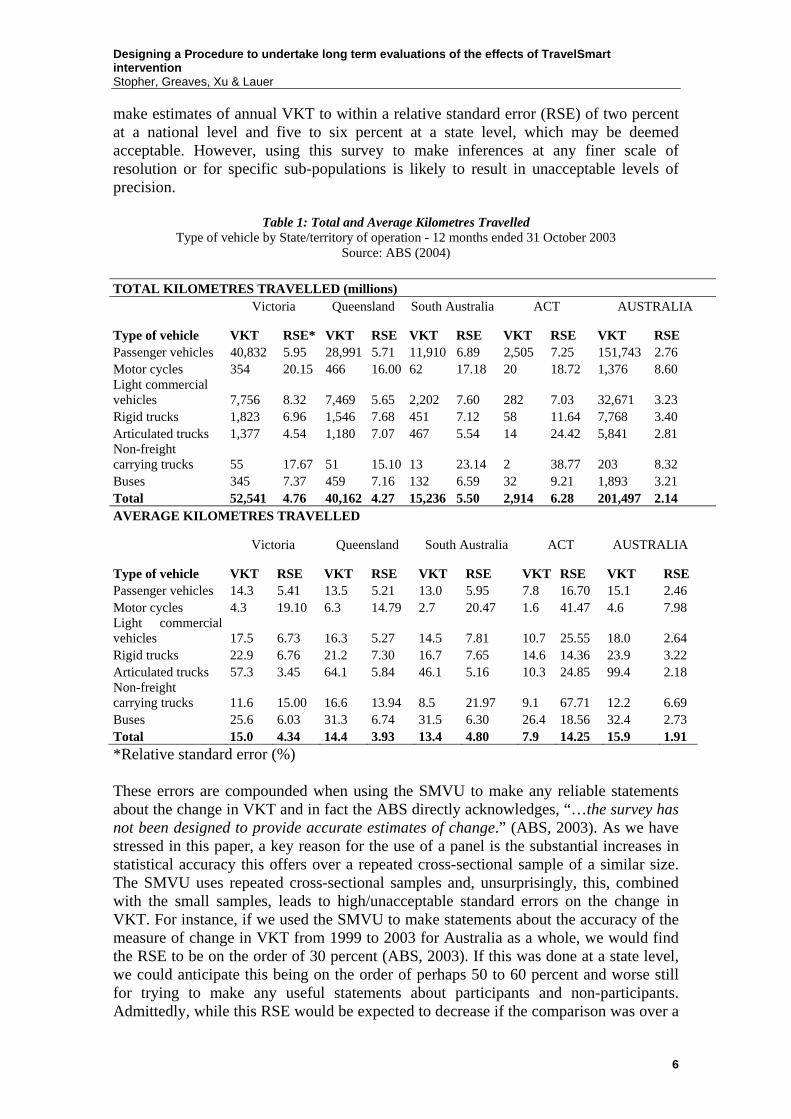
make estimates of annual VKT to within a relative standard error (RSE) of two percent at a national level and five to six percent at a state level, which may be deemed acceptable. However, using this survey to make inferences at any finer scale of resolution or for specific sub-populations is likely to result in unacceptable levels of precision.

Table 1: Total and Average Kilometres Travelled Type of vehicle by State/territory of operation - 12 months ended 31 October 2003

Source: ABS (2004) TOTAL KILOMETRES TRAVELLED (millions) Victoria Queensland South Australia ACT AUSTRALIA

Type of vehicle VKT RSE* VKT RSE VKT RSE VKT RSE VKT RSE Passenger vehicles 40,832 5.95 28,991 5.71 11,910 6.89 2,505 7.25 151,743 2.76 Motor cycles 354 20.15 466 16.00 62 17.18 20 18.72 1,376 8.60 Light commercial vehicles 7,756 8.32 7,469 5.65 2,202 7.60 282 7.03 32,671 3.23 Rigid trucks 1,823 6.96 1,546 7.68 451 7.12 58 11.64 7,768 3.40 Articulated trucks 1,377 4.54 1,180 7.07 467 5.54 14 24.42 5,841 2.81 Non-freight carrying trucks 55 17.67 51 15.10 13 23.14 2 38.77 203 8.32 Buses 345 7.37 459 7.16 132 6.59 32 9.21 1,893 3.21 Total 52,541 4.76 40,162 4.27 15,236 5.50 2,914 6.28 201,497 2.14 AVERAGE KILOMETRES TRAVELLED

Victoria Queensland South Australia ACT AUSTRALIA

Type of vehicle VKT RSE VKT RSE VKT RSE VKT RSE VKT RSE Passenger vehicles 14.3 5.41 13.5 5.21 13.0 5.95 7.8 16.70 15.1 2.46 Motor cycles 4.3 19.10 6.3 14.79 2.7 20.47 1.6 41.47 4.6 7.98 Light commercial vehicles 17.5 6.73 16.3 5.27 14.5 7.81 10.7 25.55 18.0 2.64 Rigid trucks 22.9 6.76 21.2 7.30 16.7 7.65 14.6 14.36 23.9 3.22 Articulated trucks 57.3 3.45 64.1 5.84 46.1 5.16 10.3 24.85 99.4 2.18 Non-freight carrying trucks 11.6 15.00 16.6 13.94 8.5 21.97 9.1 67.71 12.2 6.69 Buses 25.6 6.03 31.3 6.74 31.5 6.30 26.4 18.56 32.4 2.73 Total 15.0 4.34 14.4 3.93 13.4 4.80 7.9 14.25 15.9 1.91 *Relative standard error (%) These errors are compounded when using the SMVU to make any reliable statements about the change in VKT and in fact the ABS directly acknowledges, “…the survey has not been designed to provide accurate estimates of change.” (ABS, 2003). As we have stressed in this paper, a key reason for the use of a panel is the substantial increases in statistical accuracy this offers over a repeated cross-sectional sample of a similar size. The SMVU uses repeated cross-sectional samples and, unsurprisingly, this, combined with the small samples, leads to high/unacceptable standard errors on the change in VKT. For instance, if we used the SMVU to make statements about the accuracy of the measure of change in VKT from 1999 to 2003 for Australia as a whole, we would find the RSE to be on the order of 30 percent (ABS, 2003). If this was done at a state level, we could anticipate this being on the order of perhaps 50 to 60 percent and worse still for trying to make any useful statements about participants and non-participants. Admittedly, while this RSE would be expected to decrease if the comparison was over a



7

year from 2002 to 2003, the bottom line is it does not enable us to even say (statistically speaking) whether VKT has actually increased or decreased.

2.4 Passive Measurement - GPS Surveys A novel method of collecting the data is to use GPS devices. The use of GPS devices to track travel is a recent development, made possible with recent technology changes that have permitted devices to be developed that can be carried by individuals. ITLS has pioneered the use of these devices in Australia, both in evaluating a TravelSmart initiative and in validating household travel survey data. The advantages of the GPS are: 1. It is a passive method of data collection that requires very little from the

respondent other than carrying the device with her or him for the period requested. 2. It records data very accurately about routes used, distance travelled, time taken,

and when and where the trip takes place. 3. It provides a means to obtain travel data over a number of days, with very little

additional burden for respondents. 4. Devices will record distances for all modes of travel, and permit the analyst to

infer the mode of travel. Hence, VKT and PKT can be estimated much more accurately than from diaries, and also walk and bicycle travel can be captured.

The GPS also has disadvantages: 1. Devices can easily be left at home and not carried by the respondent. 2. Initial versions of the devices were rather cumbersome, and awkward to take with

the respondent. However, newer technology is solving this problem. A new version that is being produced in South Australia is of the size and weight of a mobile telephone, and seems likely to overcome much of this problem.

3. Devices do not record when a person is in a train, ferry, tunnel, and sometimes in a bus.

4. Devices may take time to acquire position, such that some short trips are lost altogether, and the beginning of other trips may not be recorded. However, these problems can be ameliorated through decision-making rules integrated within processing routines.

In the newest form factors, the devices are available in the shape and weight of a mobile telephone. This offers considerable potential to overcome past problems with wearable devices. At the same time, in-vehicle devices are already quite well accepted, and have been used successfully in a study in Sydney. In applications in Australia to date, the devices have been used for up to one week. New versions of the devices offer considerably better battery power and much greater memory capacity, thereby offering the potential that GPS data could be collected over weeks or even months. The main disadvantage of the method in this application is the cost. Devices cost around $950 each, and must usually be couriered to a household and back to the survey firm. There is also a significant amount of work that needs to be done to process the data and convert the information to usable statistics. This is, therefore, a very accurate method, but not a cheap method. Nevertheless, given the potential accuracy of collecting anywhere from a week to a month of travel data, the sample sizes required may be


8

substantially reduced, thereby offsetting the expense of each household in the sample. It is necessary to pursue pilot survey work with this method to ascertain the sample sizes that would be needed. Preliminary evidence suggests, however, that sample sizes as small as 100-200 households per state would be quite large enough to provide very accurate data from an annual or biannual survey.

2.5 Odometer Surveys A fourth alternative, that has not been used independently of a travel diary before, is based on using that part of the diary survey that is actually most pertinent to the measurement of VKT, which is the odometer reading. However, the proposal here is to collect odometer readings periodically from the same households, in order to be able to estimate the distances that all cars in the household have been driven over a particular time period. From this information, average VKT per day can be estimated, and comparisons can be made from one period to another, to determine if there is a trend in VKT upwards or downwards. At the same time that the odometer readings are collected, it will also be important to collect data on household and person demographics, and vehicle information. These data would then be checked again at each succeeding period, to determine if there have been changes in the household make up, person characteristics, or vehicles.

2.5.1 Benefits of Odometer Surveys The benefits of the odometer surveys are: 1. They involve very little burden for the respondent. 2. They collect only the information needed to measure changes in VKT. 3. They are not subject to error in trip reporting and also provide little opportunity

for respondents to give a “politically correct” response as opposed to a true response, particularly because it will be difficult for them to assess how they would need to lie to make the report “politically correct”.

2.5.2 Challenges with Odometer Surveys We anticipate that there will be two main problems with odometer surveys, and one or two minor problems. The most serious major problem is to get people to remember to record the odometer reading. Experience with diary surveys is that people will often remember to record an odometer reading at one time, but not at the other. In the measurement anticipated by this method, this may not be a serious issue, and we have proposed a method to help get around this problem, discussed in the following subsection (2.5.3). The second main problem is that of malfunctioning odometers. Whether mechanical or electronic, odometers do malfunction, and this could lead to lost data. One of the minor problems is that modern cars use a LCD display for the odometer reading, requiring that the ignition is on to have a display. This means that it is not



9

usually a matter of walking out to one’s car, opening the door, looking at the display, and noting it down, but that the respondent has to use the ignition key and turn on the ignition to get a reading. Another minor problem arises when a household sells an existing car and replaces it with another one. In this case, there will be a need to collect data on the final odometer reading of the sold car and the initial reading of the replacement car.

2.5.3 Strategies for Successful Odometer Surveys Bearing in mind the above issues, we propose several strategies as part of the odometer survey. First, we propose that households would be pre-notified by mail about the initial recruitment into a panel for odometer measurement. After agreeing to participate, respondents would be sent a customised postcard for each household vehicle on which to record the odometer readings of each vehicle in the household, and record the date on which the odometer reading is made. These data would then be collected by telephone or post or internet. Subsequently, at each time that the odometer readings are to be collected, households would receive a prior notification by mail or e-mail of the impending measurement of odometer readings, and would again be asked to write down the odometer readings and date. These data could again be retrieved either through a mail back option, telephone call, or respondents may go to a web site and enter the data there. Second, when households are recontacted in each period, they would be asked if they have bought or sold a car since the last time they were contacted. If so, they would be asked to look at the disposal information for the car that was sold and provide the evaluators with the final odometer reading, and also to find the bill of sale for any car purchased in the period, and provide the starting odometer reading from that. We anticipate that a special form would be designed and sent to households that they can keep on the refrigerator, or other convenient location, reminding them to note these details should they sell or purchase/lease a vehicle. It is also important to note that, because the evaluators will be collecting the data on a continuing basis from each household, the specific date on which the odometer reading is written down is not important, as long as both the date and the reading are received.

2.6 Respondent Burden The other clear intuitive appeal of moving away from a diary-based approach is reduced respondent burden. While some may argue the use of GPS is more burdensome, recent design initiatives (miniaturisation and passivity of devices) suggest this is fast becoming a redundant argument. On the downside, we recognise that the desire to form a panel for (potentially) five years or more, and to increase the length and frequency of monitoring will place significant demands on individuals. However, the odometer survey is a low burden activity, and the proposed sampling mechanism, discussed in the next section, is a way to reduce the burden of a panel survey. Even the request to carry a GPS device for a week or a month and then return it to the survey firm is a low burden activity, compared to any type of diary survey.


10

2.7 Recommended Survey Procedure Based on the above discussion, the recommended procedure is the combination of GPS and odometer surveys, in which the respondents to the GPS survey also complete odometer readings at, say three-monthly intervals. The GPS survey could be conducted every six months or annually, with the GPS activity coinciding with odometer readings. Households would be asked to provide appropriate sociodemographic information at the outset and to update this each quarter. In addition, households would be asked to provide address information for household workplaces, educational facilities used by the household, and grocery stores most frequently used. These would also be updated at the time of each wave of the GPS survey.

3. Sampling Mechanism

3.1 Repeated Cross-Sectional Samples Repeated cross-sectional samples are samples that are drawn independently from a target population at each period. Such samples are relatively cheap and easy to obtain, compared to other alternatives. However, a repeated cross-sectional sample has to be a large sample to measure small changes, because of the independence (Stopher and Greaves, 2004). We have to account for both variability between the two separate samples and the variability in VKT over time. This requires very large samples for robust inferences. In addition, such samples cannot permit any form of disaggregate analysis, in which one would compare the behaviour of a given household or small group of households over a period of time. We recommend against such samples for the long-term monitoring.

3.2 Panel Surveys Panel surveys are surveys in which the same people are surveyed on repeated occasions. We propose a panel for this project for four reasons. First, a panel design will enable the tracking of change over time for specific cohorts of households. Such a dynamic assessment of change is essential for true understanding of how sustained any changes in behaviour are. Second, because there is now no need to account for the between sample variability, the sample size required for measuring a change in behaviour is very much smaller than for the repeated cross-section (Stopher and Greaves, 2004). Third, a panel design is more conducive to the formation of Target and Control groupings, if that is the option selected for separating out exogenous and endogenous change (Section 6). Finally some evidence suggests that while initial costs of recruitment are higher, in the long-term a panel may prove a cheaper option than a cross-sectional survey with an equivalent number of respondents (Lawton and Pas, 1996; Armoogum et al, 2004). In fact, even if the unit cost per respondent is higher in a panel survey it is probable this will be outweighed by the significantly smaller sample sizes required to achieve similar levels of statistical reliability.



11

There are also known challenges associated with using panels. The first is panel attrition, whereby, for a variety of reasons, people or households that are initially recruited into the panel and agree to be part of the panel drop out prematurely. Attrition arises for a number of reasons, principally through people feeling that the task is too time-consuming or challenging, changing their minds about willingness to be involved, as well as problems of moving away from the area of concern, death, or dissolution of a household. Panel attrition in the United States has been estimated to run at a level of about 20 to 30 percent per year for diary-type surveys. Second, initial recruitment is harder and more expensive than a simple one-off cross-sectional survey. As discussed below, an incentive may be needed to have a household join the panel, and it is usually necessary to maintain contact with households to keep their interest in continuing to participate. Further, when updating characteristics from a previous wave of the panel, there is a greater analysis task in being able to retrieve and reproduce for the panel members a playback of the information provided on the last occasion. That is, to reduce respondent burden, each household is provided with a copy of their household characteristics from the preceding wave and asked if anything in the household has changed; this process requires great care and is quite labour intensive for the evaluator. Third, there may be the problem of conditioning, in which as the person or household continues in the panel, their membership of the panel may actually cause them to change the behaviours of interest. We anticipate in this case, however, there will be relatively little likelihood of conditioning. Finally, the problems caused by attrition, recruitment, and conditioning raise particular issues when it comes to the question of how the results should be used (i.e., weighted) to infer changes at the population level.

3.3 Panel Design The simplest panel design is one in which a number of participants are recruited and then this panel is maintained throughout the duration of the study. There are two possible ways to deal with the inevitable attrition that such a panel incurs. The first is to start with a panel of sufficient size that anticipated attrition will reduce the panel to the desired size by the end of the time period for which the panel will function. This is called a subsample panel. Thus, supposing that a panel of 500 households was desired for a period of 5 years, with anticipated attrition of 20 percent per annum. The initial panel would consist of 1,225 households, which would be expected to decline to 980 in the second wave, 785 in the third wave, 625 in the fourth wave, and 500 in the fifth wave. This would involve a total number of 4,115 surveys. The second method is one called partial replacement. In this method, the number of households that leave due to attrition each year are replaced by new panel members. This is called a refreshed panel. Thus, one might recruit a panel of 625 households, and expect to replace 125 households at the second and each subsequent wave. This would mean that every pair of waves would have 500 households, whose data could be compared across the two waves, although of the original 625 households, only 256 would, in this case, be expected to remain at the end of 5 waves, and to have provided data throughout the entire study. However, this would involve 3,125 surveys, or about 1,000 less than the first method. One of the major problems with the subsample panel is that by the end of the panel, the panel may be quite different from the population it is supposed to represent. This can


12

also happen in the refreshed panel, if the replacement members are selected to be as similar as possible to those lost by attrition. One method of benchmarking this is to use a design called a split panel. The split is between a cross-sectional survey and a panel. At each wave of measurement of the panel, which may be either a subsample panel or a refreshed panel, a separate cross-sectional sample is also drawn and surveyed. This provides greater accuracy about the changes occurring in the population, but is also a very expensive design, in that the cross-sectional sample must still be fairly large, and the panel size cannot be reduced significantly. A variant on the split panel is where the cross-sectional survey is conducted less frequently than the panel waves. However, this loses much of the benefit of the split panel, and is useful only as an occasional check on the make up of the panel. The fourth alternative panel design is known as a rotational panel. This is a panel that is conducted over a number of waves, and is used to recognise the attrition that will occur. In a rotational panel, members are recruited to the panel for a pre-defined amount of time, which is less than the time for which the panel is intended to operate. For example, in the United States, there is a rotational panel used by the Bureau of the Census for a quarterly income and expenditure survey of households, which is a continuing panel. Households are recruited for this survey and asked to remain in the panel for a period of about three years. At the end of three years, the household is replaced. The rotation is designed in such a way that only a fraction of the panel is replaced at each wave. This, then, constitutes something more like a series of overlapping panels. The three major advantages of this type of panel are that:

1. It puts a limit on the total burden to participants of being in the panel. 2. It can be used to maintain representation of the population by selective

replacement at each rotation. 3. The design minimises conditioning, by keeping respondents in the panel

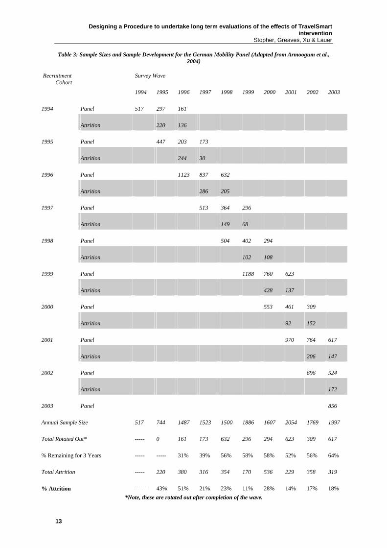
usually for a short enough time that conditioning is relatively minor. An additional benefit for this application is that it would be possible to ask questions about TravelSmart initiatives as households leave the panel, which would not be advisable in the subsampled or refreshed panels, because such questions could contaminate the panel. To demonstrate one way in which a rotational panel has operated, consider the German Mobility Panel, which is the only ongoing large-scale transportation panel that employs this particular design (Armoogum et al., 2004). Established and rigorously tested in the early 1990s, this panel became operational in 1994 and has now completed eleven waves. The survey is conducted annually over a two-month period between mid-September and mid-November and involves panel participants completing a one-week travel diary. The objective is to have households remain in the panel for three years at which point they are rotated out and refreshed with a new cohort of households. New households are also recruited to account for the inevitable attrition from households not staying in for the desired three waves. Table 3 shows how the sample has developed over the ten years of the survey.



13

Table 3: Sample Sizes and Sample Development for the German Mobility Panel (Adapted from Armoogum et al., 2004)

Survey Wave Recruitment Cohort

1994 1995 1996 1997 1998 1999 2000 2001 2002 2003

Panel 517 297 161 1994

Attrition 220 136

Panel 447 203 173 1995

Attrition 244 30

Panel 1123 837 632 1996

Attrition 286 205

Panel 513 364 296 1997

Attrition 149 68

Panel 504 402 294 1998

Attrition 102 108

Panel 1188 760 623 1999

Attrition 428 137

Panel 553 461 309 2000

Attrition 92 152

Panel 970 764 617 2001

Attrition 206 147

Panel 696 524 2002

Attrition 172

2003 Panel 856

Annual Sample Size 517 744 1487 1523 1500 1886 1607 2054 1769 1997

Total Rotated Out* ----- 0 161 173 632 296 294 623 309 617

% Remaining for 3 Years ----- ----- 31% 39% 56% 58% 58% 52% 56% 64%

Total Attrition ----- 220 380 316 354 170 536 229 358 319

% Attrition ------ 43% 51% 21% 23% 11% 28% 14% 17% 18% *Note, these are rotated out after completion of the wave.


14

Table 1 shows that 517 households were initially recruited in 1994 but 220 households (43%) dropped out of the survey, leaving 297 to complete the 1995 wave. At this stage an additional 447 households were recruited bringing the total sample size for that year to 744 households. In 1996, a further 136 households in the initial cohort and 244 households in the 1995 cohort dropped out representing a total attrition of 380 households (51%). A further 1,123 households were recruited, bringing the total sample to 1,487 households. After this wave, we see the first instance of rotation out of the panel, in this case the 161 remaining households from the 1994 cohort – this translates to 31% of households remaining in the survey for the desired duration. As the survey has continued, it is clear that attrition has been reduced substantially since 1996 and the numbers staying in for the three years has increased (to as much as 64% from the 2001-2003 cohort). There are also some caveats behind the figures – for instance the large recruitment in 1999 was due to the expansion of the survey into the former East Germany.

3.4.1 Attrition Reduction Strategies The main reasons for attrition in a panel are usually non-response (a decision to terminate participation in the panel prematurely), loss of interest, death, moving away from the target area, and dissolution of a household, when households are the unit being sampled. In this survey, it is unclear whether or not households should be followed to wherever they move in Australia. Because the VTBC strategies are aimed at changing individuals’ travel behaviour patterns, it could be argued that they should continue to be part of the panel so long as they are in Australia. On the other hand, moving away from the area where the travel behaviour change tools were provided may reduce the ability of a household to continue to maintain the behaviours learnt from the intervention. We recommend that “moving away”, when it means moving out of the immediate vicinity of the original residence should result in removal from the panel. Of course, there is nothing that can be done in the instance of death of a household, although death of one member of a multi-person household should not change panel membership, unless the wishes of the remaining household members are to leave the panel. Dissolution of a household from death, divorce etc, should be handled as follows: any new household formed from the original household within the same vicinity as the original one should, if possible, be retained in the panel. Any new household that is formed elsewhere should be treated the same as moving away. In many instances, however, members of a household that has dissolved will not wish to continue with the panel, and their wishes must be respected. Non-response, fatigue, and loss of interest are the major forms of attrition that can be mitigated. In the past, it has been found that continued contact with the household, and sharing of results with the household help to maintain interest and reduce non-response. We propose, therefore, that a series of re-contacts should be planned for each household. This would include sending Christmas or Holiday greetings around the Christmas/New Year season, sending birthday greetings to household members at the appropriate time, and providing information back to the household as to observed travel patterns.



15

A second method to reduce non-response and loss of interest is that the requests for participation in the household will be made every three months. This frequency of contact should help to keep people more interested and involved in the panel. Also, for those households that are contacted by telephone, we recommend that the same interviewer contact the household each time, so that a rapport will be built up between the interviewer and the household – empirical evidence has shown this issue of interviewer maintenance (which is easily over-looked) to be of extreme importance in maintaining panel participation (Hensher, 1987). The third method is to provide incentives. This is discussed in the section on incentives.

3.4.2 The Importance of Recruitment Recruiting participants into a panel is clearly more challenging than for a traditional cross-sectional survey because of the extra respondent burden. While we tend to focus on recruitment in terms of numbers who enter the panel, evidence suggests that how respondents are recruited can have a significant impact on (ultimately) keeping them in the panel. The German Mobility Panel, for instance, employs a very stringent pre-selection process when refreshing the sample and will only recruit ‘reliable’ respondents into the panel who would participate for the entire three years (Kuhnimhof and Chlond, 2003). It appears that this strategy does provide long-term benefits in terms of the stability of the panel, although this process has to be undertaken with extreme caution, because of potential bias in the final make-up of the sample.

3.4.3 Incentives Some form of incentive is probably worth considering, although one has to be careful that the incentive encourages participation in the survey, not that it influences behaviour. Unfortunately, the evidence is extremely limited on all these issues – it may be that pilot tests of the value of incentives and their use should be conducted. Based on what is known about incentives (Dillman, 1991; Kalfs & van Evert, 2003; Tooley, 1996; Zmud, 2003), the incentive should be fairly small, so as not to connote bribery, should be provided prior to completion of the task, and must be unrelated to the purposes of the survey. Providing free bus tickets, or coupons for reduced petrol prices would be inappropriate for this survey. The types of incentives that might be considered are such things as a small monetary gift, grocery discounts, discounts for hardware stores or CDs, etc. It might be worthwhile to assemble a set of possible incentives and then offer households, at the time of recruitment (and perhaps at each subsequent contact) a choice of the type of incentive they would like to receive.

3.5 Recommended Sampling Mechanism The recommended sampling mechanism is to use a rotational panel, in which panel members are asked to remain in the panel for three years. In the first two years, replacement is undertaken only for attrition. At the end of the third year, all households remaining from the initial recruitment would be rotated out of the panel, and replaced with new panel members, together with any attrition from the replacements of the preceding two years.


16

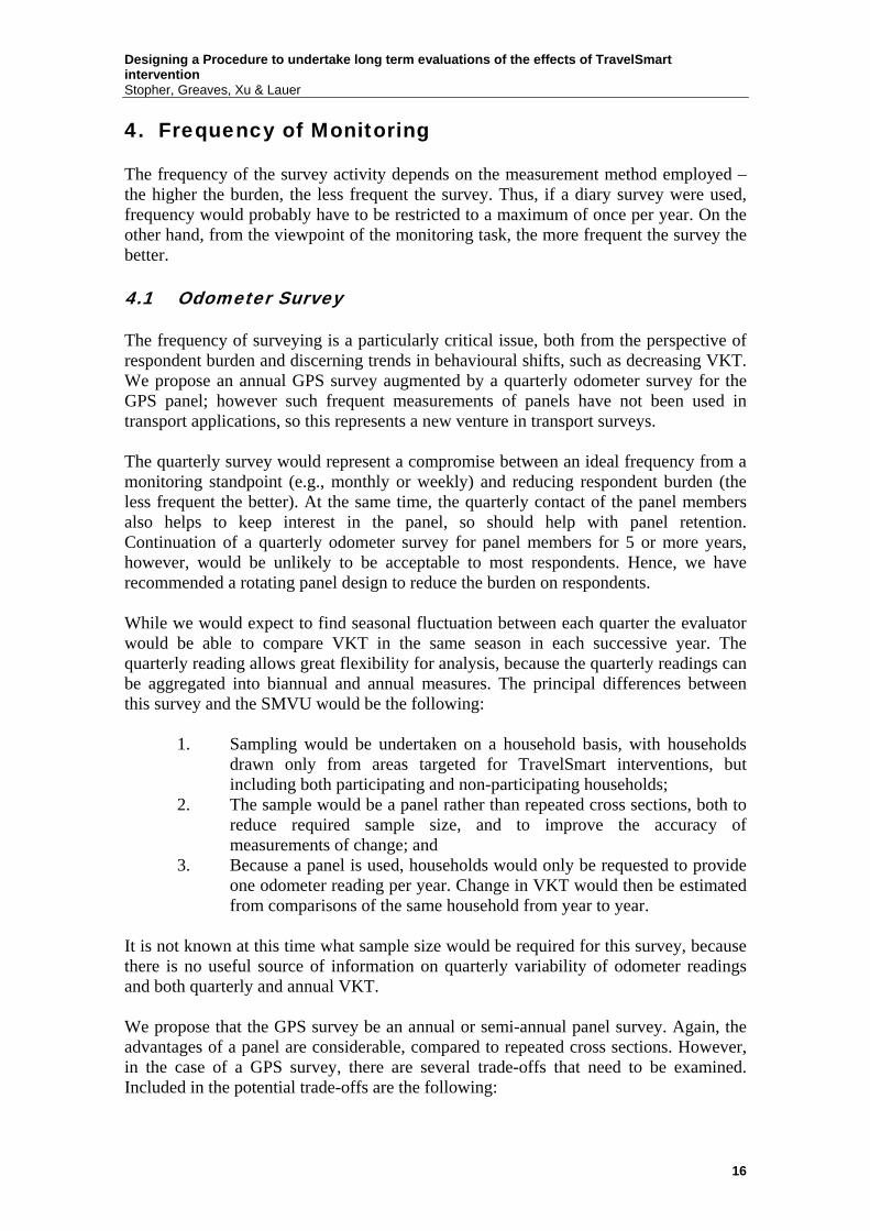
4. Frequency of Monitoring The frequency of the survey activity depends on the measurement method employed – the higher the burden, the less frequent the survey. Thus, if a diary survey were used, frequency would probably have to be restricted to a maximum of once per year. On the other hand, from the viewpoint of the monitoring task, the more frequent the survey the better. 4.1 Odometer Survey The frequency of surveying is a particularly critical issue, both from the perspective of respondent burden and discerning trends in behavioural shifts, such as decreasing VKT. We propose an annual GPS survey augmented by a quarterly odometer survey for the GPS panel; however such frequent measurements of panels have not been used in transport applications, so this represents a new venture in transport surveys. The quarterly survey would represent a compromise between an ideal frequency from a monitoring standpoint (e.g., monthly or weekly) and reducing respondent burden (the less frequent the better). At the same time, the quarterly contact of the panel members also helps to keep interest in the panel, so should help with panel retention. Continuation of a quarterly odometer survey for panel members for 5 or more years, however, would be unlikely to be acceptable to most respondents. Hence, we have recommended a rotating panel design to reduce the burden on respondents. While we would expect to find seasonal fluctuation between each quarter the evaluator would be able to compare VKT in the same season in each successive year. The quarterly reading allows great flexibility for analysis, because the quarterly readings can be aggregated into biannual and annual measures. The principal differences between this survey and the SMVU would be the following:

1. Sampling would be undertaken on a household basis, with households drawn only from areas targeted for TravelSmart interventions, but including both participating and non-participating households;

2. The sample would be a panel rather than repeated cross sections, both to reduce required sample size, and to improve the accuracy of measurements of change; and

3. Because a panel is used, households would only be requested to provide one odometer reading per year. Change in VKT would then be estimated from comparisons of the same household from year to year.

It is not known at this time what sample size would be required for this survey, because there is no useful source of information on quarterly variability of odometer readings and both quarterly and annual VKT. We propose that the GPS survey be an annual or semi-annual panel survey. Again, the advantages of a panel are considerable, compared to repeated cross sections. However, in the case of a GPS survey, there are several trade-offs that need to be examined. Included in the potential trade-offs are the following:



17

1. Frequency of the GPS survey – this could be once or twice per year, with all panel members being surveyed at approximately the same time, or it could be spread throughout the entire year; and

2. Length of time that GPS recording is performed – this could be as little as a few days to one week, or could be as long as one month.

The longer the period for which data are recorded by the GPS device, the greater the accuracy of measurement of such variables as VKT, and therefore either the sample size required will be smaller, or the survey can be undertaken less frequently. Measuring all panel participants at the same time each year provides for accurate information on VKT change from year to year. However, measurement throughout the year allows a more accurate estimate to be made of annual VKT (because there is information on seasonal variation), and therefore total greenhouse gas emissions. Measuring panel participants twice per year, with measurements spread through the entire year will provide increased accuracy on annual VKT and emissions reductions, without requiring the large number of devices that would be required if all panel members were to be surveyed within a period of a month or two. Again, sample sizes are not known at this time, because there is too little available information on variability in VKT measurement from GPS, and there is no information available from measurement over a period as long as one month. However, in terms of relative sample size, the largest sample size would be required if all households were instrumented for one week once per year, and the costs for his would be highest if all households are surveyed at the same time of the year and lowest if the survey is spread throughout the entire year. The smallest sample size requirements would be sampling households twice per year, and with each household keeping the devices for one full month. The costs for this would again be highest if all households are surveyed in the same period of the year and lowest if the sampling is spread throughout the six month period. Also, by using the odometer survey in conjunction with the GPS, we are able to obtain some information on seasonal variation, as well as validation of the car element of VKT measured by the GPS devices.

5. Sampling Method

5.1 Recruitment/Delivery Method Our recommendation for the odometer survey is to start with a pre-notification letter, and follow this with a telephone contact of all households for which a telephone number is available. For households where no telephone number is available, we would propose that a face-to-face contact should be made. For workplaces, where e-mail address lists can be provided by the employer/owner, e-mail contact may be made for the pre-notification letter, but either telephone or face-to-face recruitment is probably necessary for maximum effectiveness. Subsequent contact can be at the choice of the recruited households, with the choices including telephone, face-to-face, mail, e-mail, and Internet. As noted previously, however, each quarterly wave of the panel should involve a pre-notification letter or card that would be sent by mail.


18

We also recommend that the pre-notification letters be sent using Express Post, to increase the likelihood that people will open the letter and read it, and to convey the importance of the survey. This will also provide better information on households that move away. The cost of this form of postage is only marginally greater than using regular postage, especially when purchased in bulk quantities.

5.2 Stratification Schema We propose that a multi-stage stratified sample of households be drawn for the monitoring panel. The first stage of sampling should be to sample suburbs that have been identified as candidate suburbs for inclusion in the study. The suburbs should be classified first into categories describing their proximity to the CBD of the metropolitan area, e.g., inner, middle, and outer. Suburbs should also be classified by state or territory. The first stage sample would then be a random stratified sample of suburbs, so that each type of suburb in each state is included in the first stage sample (i.e., an inner, middle, and outer suburb in each state and territory). Whether more than one suburb should be sampled in each category should be determined based on the sample size needs, budget, and number of eligible suburbs in total. The second stage will be to sample households from within each suburb. Again, a stratified sample is recommended, with the strata being defined by household size and vehicle availability (two measures that correlate highly with the amount of travel undertaken), and also by whether or not the household originally took up TravelSmart opportunities. The former attributes will probably need to be established at the time of recruitment. However, the latter should not be ascertained by questioning the household, but should be determined by using the lists of households that were originally approached and which agreed to participate in the TravelSmart initiative. To avoid contamination, it is important that the monitoring is done without mention of, or any reference to TravelSmart. Once the overall sample size is determined, it will be possible to establish the size of the samples within each suburb. It is probably ideal if the sample contained equal numbers of households in each suburb, and equal numbers in each household classification (e.g., household size by vehicle ownership by participation in TravelSmart). Equal size samples in each category would ensure that there will be similar levels of accuracy in measuring changes in VKT (or lack of change) over the duration of the monitoring program.

5.3 Sample Size Requirements Establishing the sample size requirements to achieve an acceptable level of statistical accuracy is clearly a fundamental component of the design any monitoring program. The first problem is defining what represents an acceptable level of accuracy in this case. Because it is unclear what size of change, if any, we may wish to establish, this is not a trivial task. However, it may be appropriate to start by proposing to measure changes in VKT from year to year with an accuracy of ±1 percent with 95 percent confidence. This would mean that, if the change in VKT was measured as zero, we would have 95 percent confidence that it was between -1 percent and +1 percent. If the



19

change measured was 2 percent, we would have 95 percent confidence that the real change was between 1 and 3 percent. In this latter case, this would mean that we would have better than 95 percent confidence that the change was not zero percent or negative, and also that it was not as much as, say 4 percent. Whether or not this is an acceptable level of accuracy has to be determined by those for whom the evaluation is being done. The implications with respect to sample size and, therefore, cost, cannot be ascertained at this time, for reasons that are explained subsequently. It will then have to be determined as to whether this level of accuracy applies to the entire monitoring sample, or is to be achieved on a state by state basis, or suburb by suburb. In addition, it will be necessary to determine if comparisons are to be made between, say, households that took up TravelSmart and households that did not. In this case, is the same level of accuracy required for the comparison between these two groups? Also, is this comparison to be run at the level of the total sample, or state by state, or even suburb by suburb? These are questions that must be answered by the evaluation sponsors. The critical measure for determining sample size is the variability in the item to be measured, and the covariance or correlation of that item between the panel waves. Because time series data on odometer readings does not appear to have been obtained at a quarterly level, there is no information available currently on the size of the variance of VKT per quarter, nor is there any indication of the correlation between measurements over time. Because we do not know the variability that can be expected in an odometer survey, we do not know at this stage what the variability in VKT will be, which is pivotal to the calculation of sample sizes required for statistically valid results. A pilot study would be required before a useful estimate of sample size could be produced. As this is pioneering research, there is much that we simply do not know about what to expect. Once there is available information on the variability of odometer readings or, perhaps preferably, VKT per day per household, a set of estimates of sample sizes can be determined for different levels of accuracy. This can then be used to determine an acceptable sample size.

5.4 An Hypothetical Example of Application of the Sampling Scheme It seems that it would be useful to illustrate how all of this would work, by using a set of hypothetical numbers and conditions. It must be stressed that this is purely hypothetical, and that the actual application of the sampling scheme may prove very different from this example. Suppose that it was determined that a sample of 3,000 households was required for the desired level of accuracy. Suppose also, that the numbers of suburbs in each state by urban location that have been targeted for TravelSmart interventions within the program are as shown in Table 4.


20

Table 4: Hypothetical Numbers of TravelSmart Suburbs by State/Territory State/Territory Inner Middle Outer Total ACT 3 4 3 10 Queensland 7 12 6 25 South Australia 6 9 5 20 Victoria 9 14 7 30 We decide now to draw a proportionate sample from each state and locality, using a sampling rate of one in three, rounded to the nearest integer. This results in the sample of localities shown in Table 5. This gives 28 suburbs in the final sample. From these 28 suburbs, we will sample an equal number of households, in order to provide close to similar accuracy about each. With a goal of 3,000, we need about 107 from each suburb, so choose to sample slightly more from each at 110, yielding a total sample of 3,080 households.

Table 5: Hypothetical Numbers of TravelSmart Suburbs and Household Sample Sizes by State/Territory

State/Territory Inner Middle Outer Total Suburbs Sample Suburbs Sample Suburbs Sample Suburbs SampleACT 1 110 1 110 1 110 3 330 Queensland 2 220 4 440 2 220 8 880 South Australia

2 220 3 330 2 220 7 770

Victoria 3 330 5 550 2 220 10 1100 TOTAL 8 880 13 1430 7 770 28 3080 As shown in Table 5, such a procedure would also provide a state-by-state sample of 330 for the ACT, 880 for Queensland, 770 for South Australia, and 1,100 for Victoria. Other strategies are also possible, depending on the goals of the sponsors. For example, the sample could have been split equally between each of the states and territories, so that each one received a sample of 750, in this case. Then, the option is either to sample equal numbers of suburbs from each, or to use different sampling rates in each suburb. As noted, however, households should be sampled to give a representation of each household size and vehicle availability combination and to represent both households that participated in TravelSmart and those that did not. Thus, for each suburb, the sampling strata might be as shown in Table 6. Note that zero car owning households are not included, because they will not have odometers to be surveyed, and they are also, presumably, not participants in TravelSmart initiatives. It may be necessary to obtain an estimate of the proportion of such households in each sampled suburb, so that correct expansion of the results can be made to the total population of the partner states and territories. The sample sizes could be set proportionally to their occurrence in the suburb, or they could be set equal in all cells, or they could be set to produce identical error levels in each cell. Given a sample size of about 110 for a suburb, an equal sample in each cell would consist of about 6 households in each cell. It may also be necessary to combine



21

some cells further in this distribution, because it will be relatively hard to find households with more than four persons. The actual sample size (3,000 in this hypothetical case) would have to be determined from the variability of the VKT measures and the desired level of accuracy. If individual states desire a certain level of accuracy, then this would override the computation. The desired accuracy will have a profound impact on the necessary sample sizes for the monitoring program and for very accurate results the sample could be very large.

Table 6: Potential Household Stratification Scheme for Each Suburb

Household Size TravelSmart Households

Vehicles Available 1 2 3 4+ 1 s1 S2 s3 s4 2 S5 s6 s7

Yes

3+ s8 s9 1 s10 s11 s12 s13 2 s14 s15 s16

No

3+ s17 s18

6. Differentiating Sources of Change Most of the TravelSmart applications that are to be monitored in the long term are currently underway, or soon to be initiated. Therefore, it will not be possible to obtain a before data set consistent with the methodology developed for the long-term monitoring for a number of these projects, especially those underway, and those initiated before pilot surveys for the long-term monitoring are completed. (For the future, however, the long-term method should be equally applicable to short-term evaluation and the use of this method should be encouraged for that purpose to allow for consistent between-locations comparisons). Referring back to Figure 1, it is clear that there are numerous problems in actually sorting out the sources of change. Not only do certain national trends have to be taken into account, but also the individual households in the panel will not be without internal changes that may affect household VKT. For example, a household that starts the monitoring period with three children aged 13, 12, and 9 would end the monitoring period with children aged 18, 17, and 14, with the likelihood that the two older children would be licensed to drive by then, and that the household may have acquired one or more additional vehicles. While our recommended procedure would not follow this household from the beginning to the end of the monitoring period, if the household were to enter in the last two years, not only might its VKT be substantially higher than it would have been at the time of the TravelSmart intervention, but its VKT may also be growing more rapidly than the average, because of the addition of the two teenagers as active drivers. External factors refer to all the factors other than the intervention, which could potentially impact travel, such as changes in the participants’ circumstances (e.g.,


22

change in family structure, acquisition of a new car), the transport system (new tolls, fare rises), or the wider economy (increased petrol prices, increased unemployment, etc.). In the context of TravelSmart evaluations, these factors make it increasingly difficult to identify changes due directly to the intervention, something which will clearly become more troublesome the longer the monitoring period. This problem seems to provide further rationale for increasing the frequency of monitoring. The review of the health literature and our own knowledge of TravelSmart evaluations, suggests sample contamination is a serious problem when trying to definitively identify the change attributable to an intervention policy. The primary means to overcome this is through the definition of a Control Group, which is simply a physically separate segment of the population, chosen to match the Target group in terms of demographics, public transport accessibility, location to employment, etc. The identification of the population to use as a control has been contentious (e.g., Stopher and Bullock, 2001). Another serious issue with control groups has been the much lower response rates than the Target sample, especially without the use of incentives to encourage completion. The problem is made doubly difficult, because of the express intent of encouraging diffusion and the simple fact that the length of the program increases the probability that people will be exposed to it. It will generally not be feasible to follow single households and document the changes made by that household over time, for two principal reasons. First, changes taking place in the situation of a single household will be far too complex to be able to determine what long-term effects TravelSmart initiatives have had. To do this, one would need to be able to measure identical households going through identical changes, where some households were exposed to TravelSmart and others were not. Because of the huge number of possible situational changes that could occur over the monitoring period, this would simply not be feasible. Second, the rotating panel design will not permit tracking individual households throughout the monitoring period. Each household would only be monitored for a maximum of two years. In addition, describing the changes on a household-by-household basis has not been done, even for short-term monitoring; rather change has been estimated on a suburb basis, or even for an entire area covered by TravelSmart initiatives. It will be necessary to decide whether it is desired to be able to estimate long-term response to TravelSmart at a suburb-by-suburb level, at a state or territory level, or for the combination of states and territories involved. This will dictate the sample sizes that must be used. Certainly, with the sample sizes discussed in section 5.4, it is unlikely that change could be estimated at a suburb-by-suburb level; larger sample sizes would almost certainly be needed. To determine how TravelSmart households are behaving compared to those that were not exposed, there are three possible approaches. The first is to use a control group sample. The major problems with control group samples for this exercise are that the control groups must be carefully chosen to have similar characteristics to the target groups, not only in terms of household and person demographics, but also in terms of transport service levels (especially public transport, bicycle, and walk), and also be similarly located with respect to the city centre. As TravelSmart is implemented on a more and more widespread basis, this will become increasingly difficult to achieve. Indeed, since it has already been established that inner city suburbs are more responsively to TravelSmart than outer suburbs, it is possible that all inner city suburbs in all major metropolitan areas will be exposed to TravelSmart initiatives within the



23

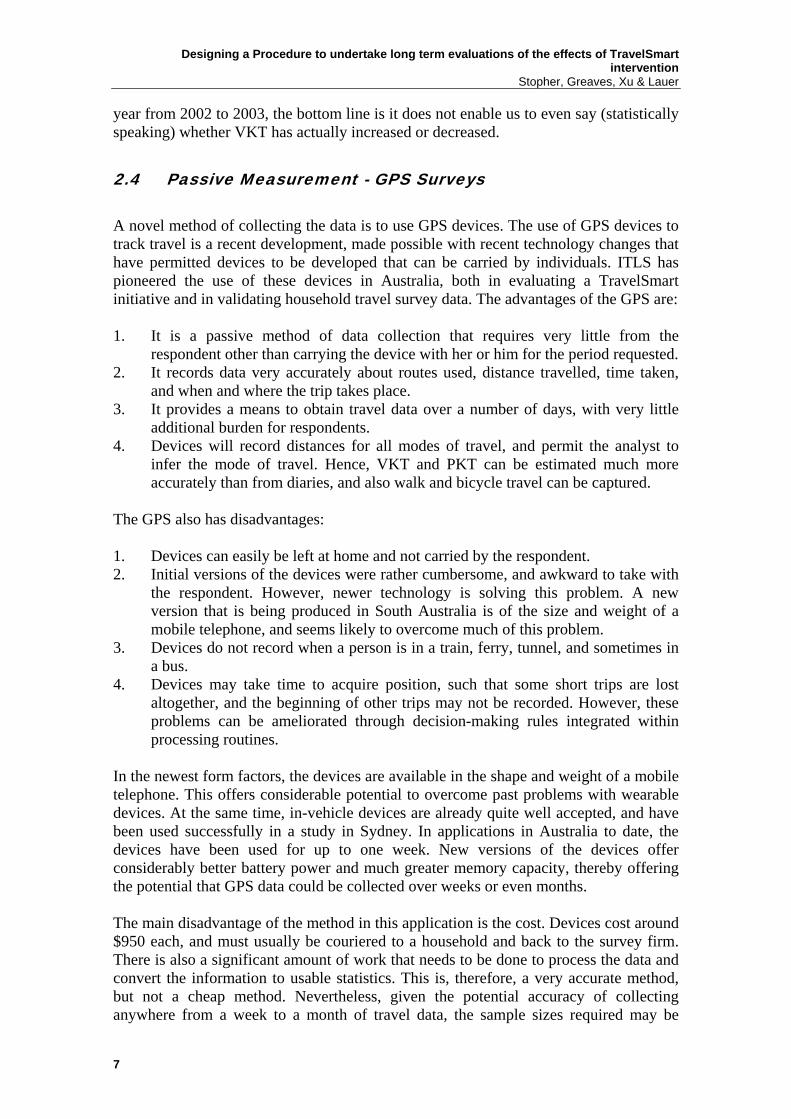
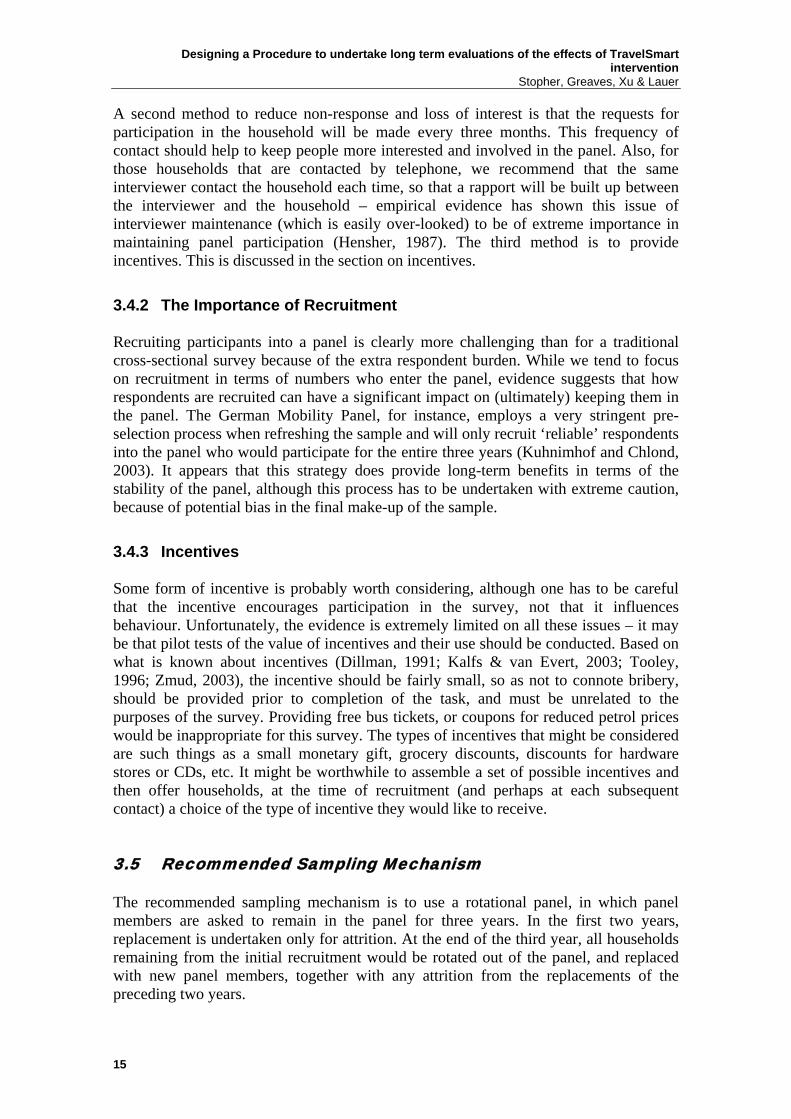
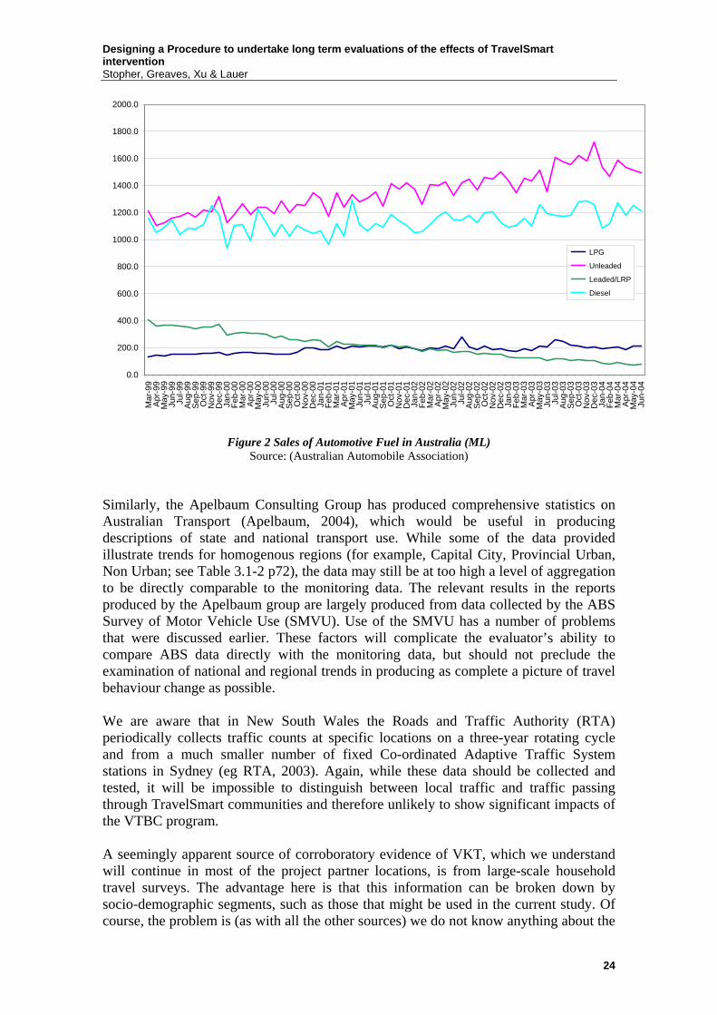
time frame of this long-term monitoring project, thereby leaving no possible control group sample for inner city suburbs. The second method is to use the non-participating households as a comparison base. This provides a better approximation to the households that do participate, but risks inclusion of diffusion effects. Overall, however, this is probably a more practical solution than the choice of control group samples, per se. The third approach is to start monitoring before the implementation of TravelSmart, and to do so sufficiently far in advance to be able to establish the trends in VKT prior to a TravelSmart intervention. In conjunction with the measurement in each suburb of participating and non-participating households, the trends of VKT in each of these two cohorts could be determined and compared, and estimates of the comparative reductions in VKT of TravelSmart households could be determined, together with an estimate of diffusion effects and their longevity in the non-participating households. We believe that this approach is actually the best of the three, but requires that monitoring begin immediately, and that it continues through the end of the long-term period. Alternatively, since most implementations involve short-term monitoring, it would be important that the short-term monitoring is done in a manner consistent with the recommended long-term monitoring strategy, and that before measurements take place as early as possible in all cases. Furthermore, before measurement should be instituted as soon as possible for all suburbs that are expected to be included in TravelSmart initiatives eventually, so that trends can be established. In practice, it is likely that a combination of these methods could be applied for evaluating change. 7. Corroboratory Evidence The challenges with attempting to ascertain the long-term effectiveness of TravelSmart interventions at a household level strongly suggest objective corroboratory evidence of sustained change on a more aggregate level is an essential part of this process. There are a number of additional sources of data relating to vehicle use that require examination within the context of the long-term monitoring program. We would encourage the collection of any data that is indicative of the volume of vehicle use. However, at this stage we expect that corroboratory evidence will not be able to be used to confirm or reject the findings of the monitoring program statistically. It will not be possible for the evaluators to separate the influences of large scale economic, structural, or social change from that produced by the implementation of TravelSmart programs. It will rather be limited to simply supporting, opposing, or overwhelming any sustained change that is measured. One of the major problems that will be encountered in the use of corroboratory data is that the level of aggregation will be too large to perceive any impact of the TravelSmart program. For example, we can locate national petrol sales data (Figure 2), which show a general upward trend, but the 2-10% behaviour change in TravelSmart communities would be completely imperceptible within this data set. The acquisition of data at the level of the community in which TravelSmart has been implemented would be most useful: that is, at a suburb, city or regional level.


24

0.0

200.0

400.0

600.0

800.0

1000.0

1200.0

1400.0

1600.0

1800.0

2000.0

Mar

-99

Apr

-99

May

-99

Jun-

99Ju

l-99

Aug

-99

Sep

-99

Oct

-99

Nov

-99

Dec

-99

Jan-

00Fe

b-00

Mar

-00

Apr

-00

May

-00

Jun-

00Ju

l-00

Aug

-00

Sep

-00

Oct

-00

Nov

-00

Dec

-00

Jan-

01Fe

b-01

Mar

-01

Apr

-01

May

-01

Jun-

01Ju

l-01

Aug

-01

Sep

-01

Oct

-01

Nov

-01

Dec

-01

Jan-

02Fe

b-02

Mar

-02

Apr

-02

May

-02

Jun-

02Ju

l-02

Aug

-02

Sep

-02

Oct

-02

Nov

-02

Dec

-02

Jan-

03Fe

b-03

Mar

-03

Apr

-03

May

-03

Jun-

03Ju

l-03

Aug

-03

Sep

-03

Oct

-03

Nov

-03

Dec

-03

Jan-

04Fe

b-04

Mar

-04

Apr

-04

May

-04

Jun-

04

LPG

Unleaded

Leaded/LRP

Diesel

Figure 2 Sales of Automotive Fuel in Australia (ML) Source: (Australian Automobile Association)

Similarly, the Apelbaum Consulting Group has produced comprehensive statistics on Australian Transport (Apelbaum, 2004), which would be useful in producing descriptions of state and national transport use. While some of the data provided illustrate trends for homogenous regions (for example, Capital City, Provincial Urban, Non Urban; see Table 3.1-2 p72), the data may still be at too high a level of aggregation to be directly comparable to the monitoring data. The relevant results in the reports produced by the Apelbaum group are largely produced from data collected by the ABS Survey of Motor Vehicle Use (SMVU). Use of the SMVU has a number of problems that were discussed earlier. These factors will complicate the evaluator’s ability to compare ABS data directly with the monitoring data, but should not preclude the examination of national and regional trends in producing as complete a picture of travel behaviour change as possible. We are aware that in New South Wales the Roads and Traffic Authority (RTA) periodically collects traffic counts at specific locations on a three-year rotating cycle and from a much smaller number of fixed Co-ordinated Adaptive Traffic System stations in Sydney (eg RTA, 2003). Again, while these data should be collected and tested, it will be impossible to distinguish between local traffic and traffic passing through TravelSmart communities and therefore unlikely to show significant impacts of the VTBC program. A seemingly apparent source of corroboratory evidence of VKT, which we understand will continue in most of the project partner locations, is from large-scale household travel surveys. The advantage here is that this information can be broken down by socio-demographic segments, such as those that might be used in the current study. Of course, the problem is (as with all the other sources) we do not know anything about the



25

level of exposure to TravelSmart interventions of participants in these surveys so we can really only use these data sources to indicate fairly aggregate trends. 8. Conclusions This paper identifies the major issues with and potential options for a long-term monitoring program of VKT over the period of the 1st Kyoto Protocol (2008 - 2013). Fundamentally, it is clear that the task is markedly different from that of a short-term before-and-after evaluation, and it brings with it additional challenges to ensure the conclusions are based on statistically reliable and robust results. In preparing and scoping the options, it is clear that much remains unknown, which will be of integral importance in the development and refinement of the final methodology for a long term monitoring program. Specifically, we argue it is necessary to investigate the following:

1. Respondent Willingness to Participate and Keep Participating. We have made an assumption that surveying respondents every three months for no more than two years is not unduly burdensome. Are our expectations accurate, or will respondents in fact be willing to stay in shorter or longer and/or participate more or less frequently? What kinds of incentives will be effective in motivating respondents to participate both initially and then on a continuing basis? What impact will the mode of recruitment and retrieval have – for instance, are modes such as e-mail, SMS, etc. seen as more acceptable than a phone call?

2. Attrition. We have assumed that there will probably be about a ten percent level of attrition from quarter to quarter. However, there is little documentation of attrition from quarterly panel surveys, and the actual level of attrition is important to establish. Furthermore, it is possible that attrition rates may decline with successive quarters (there are participants still in the Puget Sound Transportation Panel in the U.S., after 11 annual waves and the German Mobility Panel shows that attrition at the first wave is generally larger than in subsequent waves), and this would need to be known in order to design the panel correctly.

3. Length of Time in Panel. We have suggested that respondents remain in the panel for a maximum of three waves. However, this is based purely on supposition regarding respondent burden and likely willingness to continue in the panel. We do not currently know if it would be better to keep respondents in the panel for one, two or three years, or even longer. This is an issue both of respondent burden and the actual computations and sampling errors from the panel.

4. Panel Design. While we have argued here that a rotational panel is the preferred approach, much is unknown about how this should be designed specifically for this purpose. How should participants be rotated out – along the lines of the GMP or some other way?

5. Sample Size Requirements. We stressed in section 5.3 that determining the required sample sizes to achieve desired levels of statistical accuracy depends on much that is simply unknown at this stage. Fundamentally, we need to know something about the variability in odometer readings on a quarterly basis for a


26

panel, what level of statistical accuracy is required, and whether this is to apply to the entire monitoring sample, state, or suburb. A further issue is whether we should be basing sample size requirements on adjacent quarters or (recognising the probable seasonality impact) on the same quarter in the following year. Similarly, variability in GPS measurements for a week or longer are unknown, and this must also be known for sample size determination. Whether there is a significantly increased reduction in sample requirements by having the GPS task performed twice a year, or once a year for longer than a week is also unknown.

6. New Technologies. The rate of development in new technologies suggests that by the time of the start of the monitoring period, there may well be options, which were not viable at the time of writing. It is already notable, for instance, how GPS is fundamentally changing our capacity to collect travel data. It is probable that developments in mobile phone technology and vehicle electronics could offer possibilities in the future.

We envisage these issues could be investigated through a mixture of focus groups, controlled experiments, and ultimately a pilot study of the proposed methodology. Use of the methodology proposed here in short-term evaluations of TravelSmart initiatives would provide valuable information to the long-term evaluator of established trends and would be useful in the analysis of VKT variability for the determination of required sample sizes for the long term program. References

ABS (1998) Information Paper – Survey of Motor Vehicle Use: Historical Comparison. Retrieved: 9th September, 2004, from http://www.abs.gov.au/Ausstats/[email protected]/Lookup/407EBF957FC03B29CA2568A9001394D

ABS (2003) Survey of Motor Vehicle Use: 12 Months ended 31st October 2004. Retrieved: 9th September, 2004, from http://www.ausstats.abs.gov.au/ausstats/subscriber.nsf/Lookup/A97A3B6D99640F48CA256DAC000224CB/$File/92080_01%20nov%202001%20to%2031%20oct%202002.pdf

ABS (2004) Motor Vehicle Use (Survey of), Year ending October 2002 Retrieved: 1st December, 2004, from http://www.sch.abs.gov.au/SCH/A1610103.NSF/SurveysNameM?OpenView&M

Apelbaum Consulting Group Pty Ltd (2004) Australian Transport Facts 2002, Report for ATEDAC, CD-Rom.

Armoogum, J., B. Chlond, J. Madre and D. Zumkeller (2004 in press). “Panel Surveys” – A Resource Paper for the 7th ISCTSC, Costa Rica, August 2004.

Australian Automobile Association “AAA Transport Statistics Database”. Retrieved: 14th September, 2004, from http://www.aaa.asn.au/results.asp

Dillman, D.A. (1991), “The Design and Administration of Mail Surveys,” Annual Review of Sociology, 17, 225-249.



27

Hensher, D.(1987), “Issues in the Pre-Analysis of Panel Data”, Transportation Research A, 21, pp. 265-285.

Kalfs, N. and H. van Evert (2003), “Nonresponse in Travel Surveys”, in Stopher, P.R. and P.M. Jones, Transport Survey Quality and Innovation, Elsevier Press, pp. 567-586.

Richardson, A.J., Seethaler, R. and Harbutt, P. (2003) “Design Issues for Before and After Surveys of Travel Behaviour Change”, ATRF(26), CD-Rom.

RTA Traffic and Transport Directorate (2003) Traffic Volume Data for the Sydney Region 2002. Retrieved: 13th September, 2004 from http://www.rta.nsw.gov.au/trafficinformation/downloads/aadt_data_files/aadtsydney2002_i.pdf

Stopher, P. and Bullock, P. (2002) “Travel Behaviour Modification: A Critical Appraisal”, ATRF (25), CD-Rom

Stopher, P. and Greaves, S. (2004) ““Sample Size Requirements for Measuring a Change in Behaviour”, paper presented at the 27th Australasian Transport Research Forum, Adelaide, September.

Tooley, M. (1996), “Incentives and Rates of Return for Travel Surveys,” Transportation Research Record No.1551, pp. 67-73.

Upson, R. (2004). Private communication with Professor Peter R. Stopher by e-mail on 2nd December, 2004.

Wolf, J., M. Loechl, M. Thompson and C. Arce (2003). “Trip Rate Analysis in GPS-Enhanced Personal Travel Surveys”, in Transport Survey Quality and Innovation, P. Stopher and P. Jones (editors), Pergamon Press, Oxford, pp. 483-498.

Zmud, J. (2003), “Designing Instruments to Improve Response”, in Stopher, P.R. and P.M. Jones, Transport Survey Quality and Innovation, Elsevier Press, pp. 89-108.

Date post:	08-Sep-2018
Category:	Documents
Upload:	dangthuy
View:	215 times
Download:	0 times

05-11 Working Paper - University of Sydney Business...

Documents