43
J. Elder PSYC 6256 Principles of Neural Coding 9. HEBBIAN LEARNING
| Date post: | 25-May-2018 |
| Category: |
Documents |
| Upload: | doankhuong |
| View: | 225 times |
| Download: | 1 times |
J. Elder PSYC 6256 Principles of Neural Coding
9. HEBBIAN LEARNING

Probability & Bayesian Inference
J. Elder PSYC 6256 Principles of Neural Coding
2
Hebbian Learning
“When an axon of cell A is near enough to excite cell B and repeatedly or persistently takes part in firing it, some growth process or metabolic change takes place in one or both cells such that A's efficiency, as one of the cells firing B, is increased.”
This is often paraphrased as "Neurons that fire together wire together." It is commonly referred to as Hebb's Law.
Donald Hebb
Probability & Bayesian Inference
J. Elder PSYC 6256 Principles of Neural Coding
3
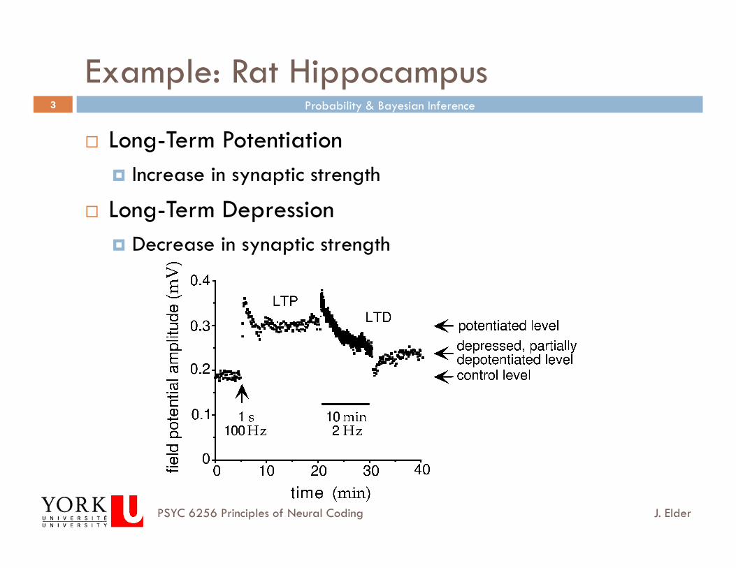
Example: Rat Hippocampus
Long-Term Potentiation Increase in synaptic strength
Long-Term Depression Decrease in synaptic strength

Single Postsynaptic Neuron

Probability & Bayesian Inference
J. Elder PSYC 6256 Principles of Neural Coding
5
Simplified Functional Model
v = wiu = w tu
v
u1 u2 uNu
Probability & Bayesian Inference
J. Elder PSYC 6256 Principles of Neural Coding
6
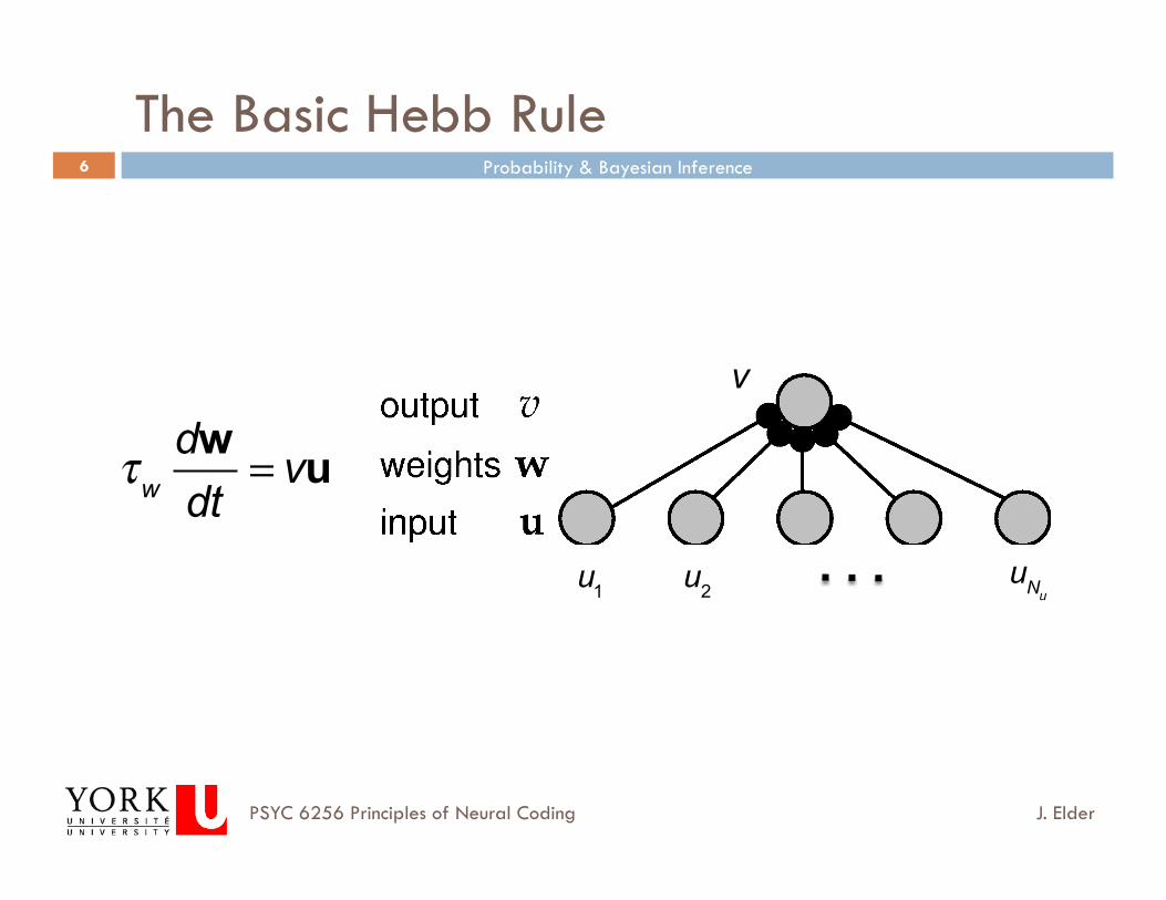
The Basic Hebb Rule
τw
dwdt
= vu
v
u1 u2 uNu

Probability & Bayesian Inference
J. Elder PSYC 6256 Principles of Neural Coding
7
Modeling Hebbian Learning
Hebbian learning can be modeled as either a continuous or a discrete process: Continuous:
Discrete:
τw
dwdt
= vu
w → w + εvu

Probability & Bayesian Inference
J. Elder PSYC 6256 Principles of Neural Coding
8
Modeling Hebbian Learning
Hebbian learning can be incremental or batch: Incremental:
Batch:
τw
dwdt
= vu
τw
dwdt
= vu

Probability & Bayesian Inference
J. Elder PSYC 6256 Principles of Neural Coding
9
Batch Learning: The Average Hebb Rule
τw
dwdt
= vu
→ τw
dwdt
= Qw
where Q = uut is the input correlation matrix
Probability & Bayesian Inference
J. Elder PSYC 6256 Principles of Neural Coding
10
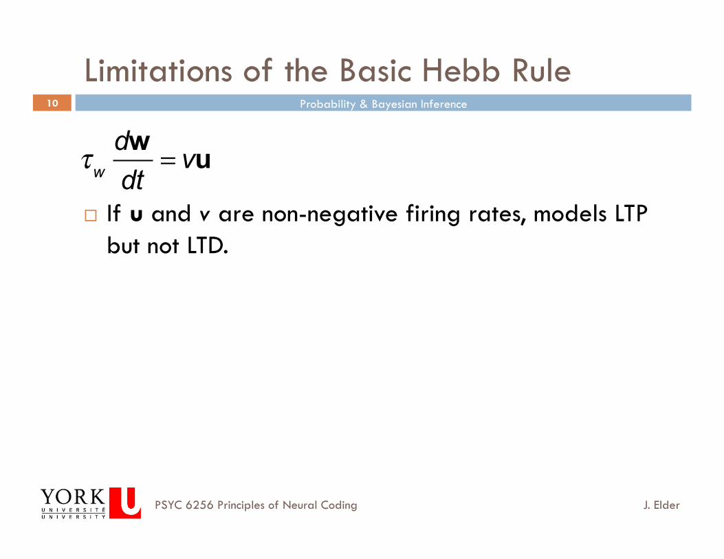
Limitations of the Basic Hebb Rule
If u and v are non-negative firing rates, models LTP but not LTD.
τw
dwdt
= vu

Probability & Bayesian Inference
J. Elder PSYC 6256 Principles of Neural Coding
11
Limitations of the Basic Hebb Rule
Even when input and output may be negative or positive, the positive feedback causes the magnitude of the weights to increase without bound:
τw
d w2
dt= 2v 2
τw
dwdt
= vu

Probability & Bayesian Inference
J. Elder PSYC 6256 Principles of Neural Coding
12
The Covariance Rule
Empirically, LTP occurs if presynaptic activity is accompanied by
high postsynaptic activity. LTD occurs if presynaptic activity is accompanied by
low postsynaptic activity. This can be modeled by introducing a postsynaptic
threshold that determines the sign of learning:
τw
dwdt
= v −θv( )u θv
Probability & Bayesian Inference
J. Elder PSYC 6256 Principles of Neural Coding
13
The Covariance Rule
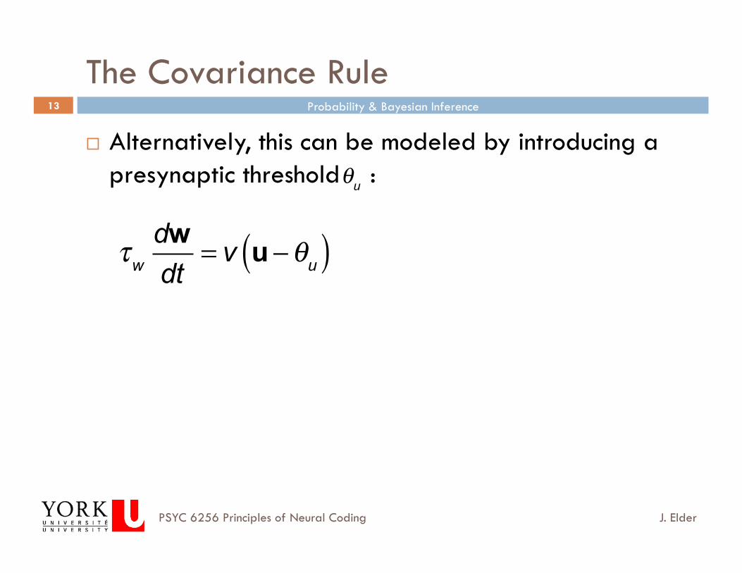
Alternatively, this can be modeled by introducing a presynaptic threshold :
τw
dwdt
= v u−θu( ) θu

Probability & Bayesian Inference
J. Elder PSYC 6256 Principles of Neural Coding
14
The Covariance Rule
In either case, a natural choice for the threshold is the average value of the input or output over the training period:
τw
dwdt
= v − v( )u
τw
dwdt
= v u− u( )or

Probability & Bayesian Inference
J. Elder PSYC 6256 Principles of Neural Coding
15
The Covariance Rule
Both models lead to the same batch learning rule:
τw
dwdt
= Cw
where C = u− u( ) u− u( )t is the input covariance matrix.
Probability & Bayesian Inference
J. Elder PSYC 6256 Principles of Neural Coding
16
The Covariance Rule
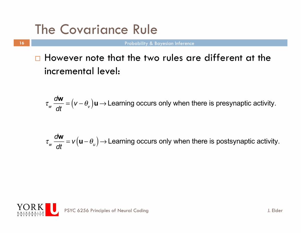
However note that the two rules are different at the incremental level:
τw
dwdt
= v −θv( )u→ Learning occurs only when there is presynaptic activity.
τw
dwdt
= v u−θu( )→ Learning occurs only when there is postsynaptic activity.
Probability & Bayesian Inference
J. Elder PSYC 6256 Principles of Neural Coding
17
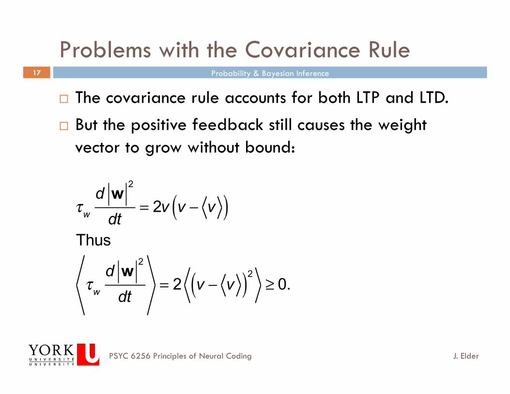
Problems with the Covariance Rule
The covariance rule accounts for both LTP and LTD. But the positive feedback still causes the weight
vector to grow without bound:
τw
d w2
dt= 2v v − v( )
Thus
τw
d w2
dt= 2 v − v( )2
≥ 0.

Synaptic Normalization

Probability & Bayesian Inference
J. Elder PSYC 6256 Principles of Neural Coding
19
Synaptic Normalization
Synaptic normalization constrains the magnitude of the weight vector to some value.
Not only does this prevent the weights from growing without bound, it introduces competition between the input neurons: for one weight to grow, another must shrink.

Probability & Bayesian Inference
J. Elder PSYC 6256 Principles of Neural Coding
20
Forms of Synaptic Normalization
Rigid Constraint: The constraint must hold at all times
Dynamic Constraint: The constraint must be satisfied asymptotically

Probability & Bayesian Inference
J. Elder PSYC 6256 Principles of Neural Coding
21
Subtractive Normalization
This is an example of a rigid constraint. Only works for non-negative weights.
τw
dwdt
= vu−v niu( )n
Nu
,
where n =11
⎡
⎣
⎢⎢⎢
⎤
⎦
⎥⎥⎥
which satisfies τw
dniwdt
= 0

Probability & Bayesian Inference
J. Elder PSYC 6256 Principles of Neural Coding
22
Subtractive Normalization
Note that subtractive normalization is non-local. τw
dwdt
= vu−v niu( )n
Nu

Probability & Bayesian Inference
J. Elder PSYC 6256 Principles of Neural Coding
23
Multiplicative Normalization: The Oja Rule
Here the damping term is proportional to the weights.
Works for positive and negative weights This is an example of a dynamic constraint:
τw
dwdt
= vu−αv 2w
τw
d w2
dt= 2v 2 1−α w
2( )
Probability & Bayesian Inference
J. Elder PSYC 6256 Principles of Neural Coding
24
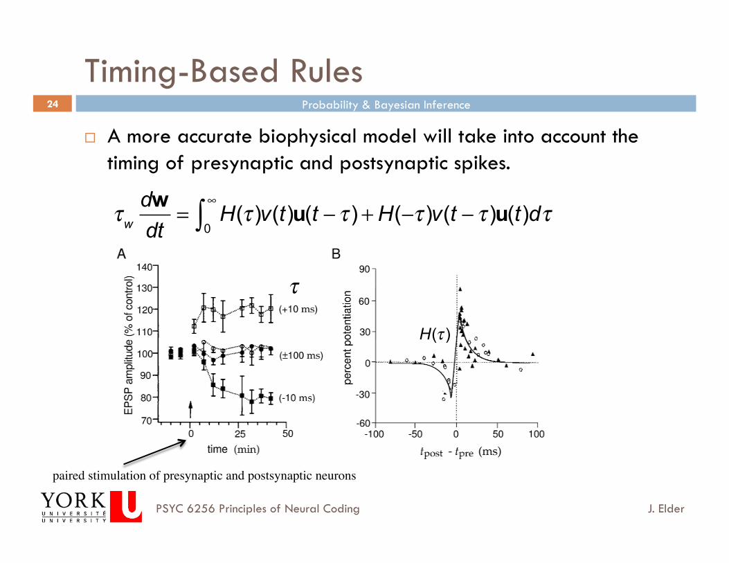
Timing-Based Rules
A more accurate biophysical model will take into account the timing of presynaptic and postsynaptic spikes.
τw
dwdt
= H(τ )v(t)u(t − τ )0
∞
∫ + H(−τ )v(t − τ )u(t)dτ
paired stimulation of presynaptic and postsynaptic neurons
τ
H(τ )

Steady State

Probability & Bayesian Inference
J. Elder PSYC 6256 Principles of Neural Coding
26
Steady State
What do the weights converge to?
τw
dwdt
= Qw
where Q = uut is the input correlation matrix
Let eµ be the eigenvectors of Q, µ = 1,2,…,Nu, satisfying
Qeµ = λµeµ
λ1 ≥ λ2 ≥λNu

Probability & Bayesian Inference
J. Elder PSYC 6256 Principles of Neural Coding
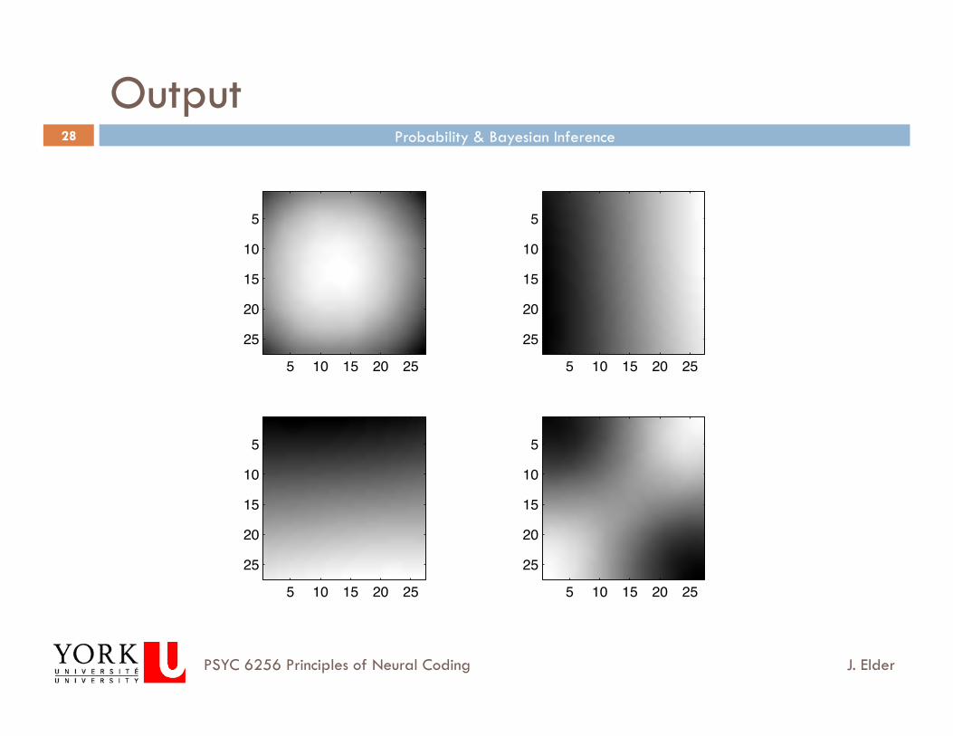
27
Eigenvectors
function lgneig(lgnims,neigs,nit) %Computes and plots first neigs eigenimages of LGN inputs to V1 %lgnims = cell array of images representing normalized LGN output %nit = number of image patches on which to base estimate
dx=1.5; %pixel size in arcmin. This is arbitrary. v1rad=round(10/dx); %V1 cell radius (pixels) Nu=(2*v1rad+1)^2; %Number of input units
nim=length(lgnims);
Q=zeros(Nu); for i=1:nit
u=im(y-v1rad:y+v1rad,x-v1rad:x+v1rad); u=u(:);
Q=Q+u*u'; %Form autocorrelation matrix end Q=Q/Nu; %normalize [v,d]=eigs(Q,neigs); %compute eigenvectors
Probability & Bayesian Inference
J. Elder PSYC 6256 Principles of Neural Coding
28
Output
5 10 15 20 25
5
10
15
20
25
5 10 15 20 25
5
10
15
20
25
5 10 15 20 25
5
10
15
20
25
5 10 15 20 25
5
10
15
20
25

Probability & Bayesian Inference
J. Elder PSYC 6256 Principles of Neural Coding
29
Steady State
Now we can express the weight vector in the eigenvector basis:
Substituting into the Hebb rule, we get
τw
dwdt
= Qw
w(t) = cµ (t)eµ
µ=1
Nµ
∑
τw
dcµ (t)dt
eµµ=1
Nµ
∑ = Q cµ (t)eµµ=1
Nµ
∑
→τw
dcµ (t)dt
= λµcµ (t) → cµ (t) = aµ exp λµ / τw( ) t( )
and thus w(t) = aµ exp λµ / τw( ) t( )eµ
µ=1
Nµ
∑
Probability & Bayesian Inference
J. Elder PSYC 6256 Principles of Neural Coding
30
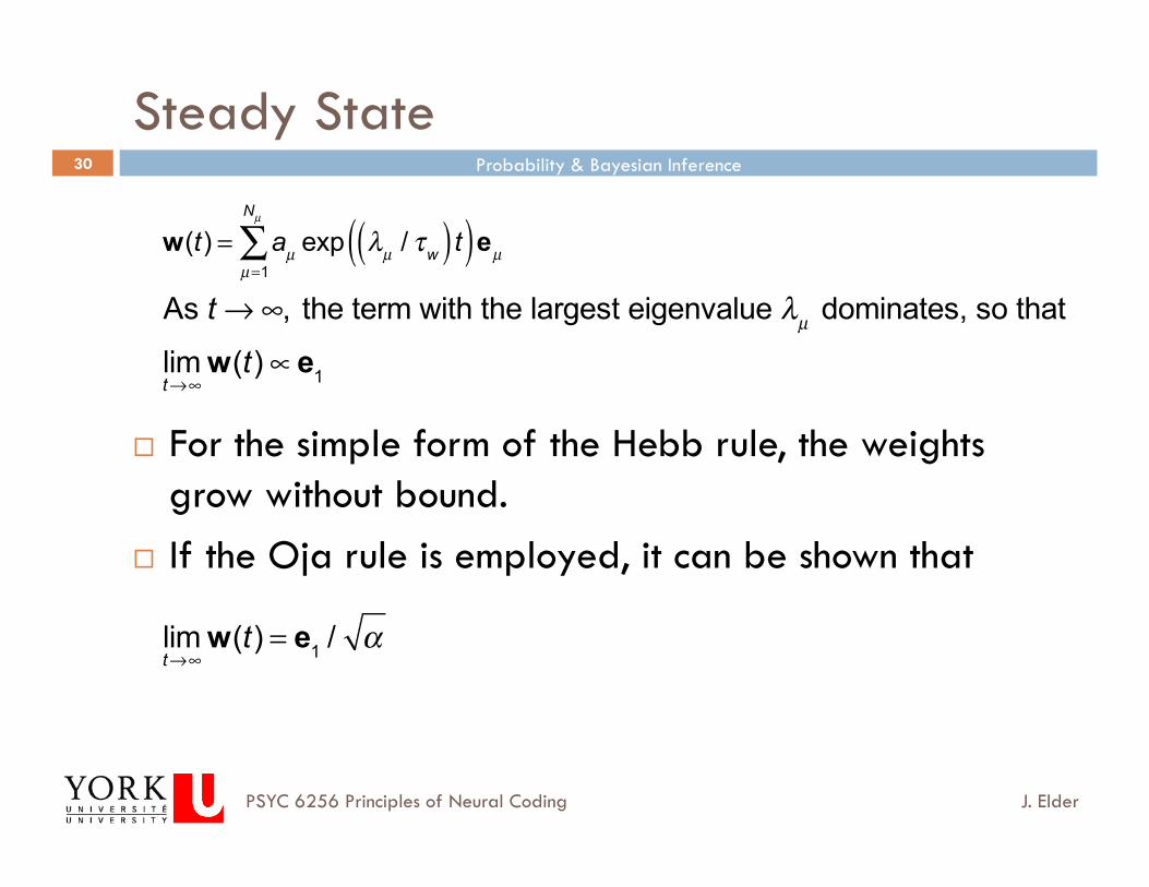
Steady State
For the simple form of the Hebb rule, the weights grow without bound.
If the Oja rule is employed, it can be shown that
w(t) = aµ exp λµ / τw( ) t( )eµ
µ=1
Nµ
∑
As t →∞, the term with the largest eigenvalue λµ dominates, so that
limt→∞
w(t) ∝ e1
limt→∞
w(t) = e1 / α
Probability & Bayesian Inference
J. Elder PSYC 6256 Principles of Neural Coding
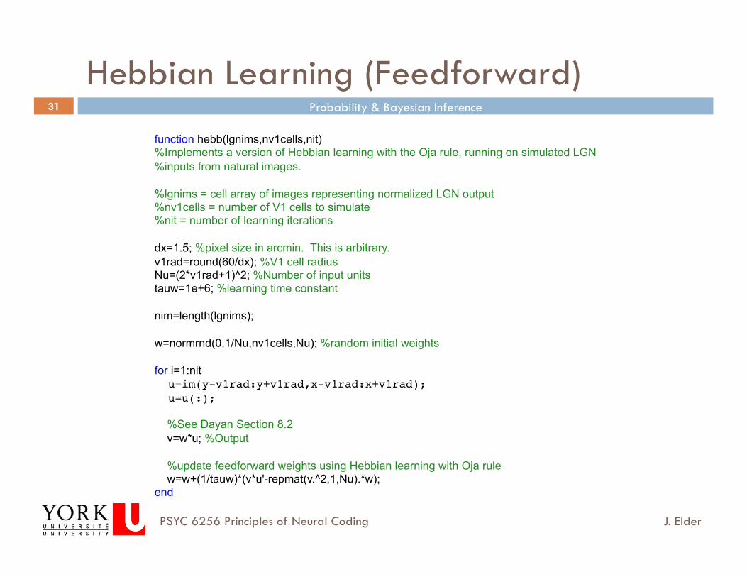
31
Hebbian Learning (Feedforward)
function hebb(lgnims,nv1cells,nit) %Implements a version of Hebbian learning with the Oja rule, running on simulated LGN %inputs from natural images.
%lgnims = cell array of images representing normalized LGN output %nv1cells = number of V1 cells to simulate %nit = number of learning iterations
dx=1.5; %pixel size in arcmin. This is arbitrary. v1rad=round(60/dx); %V1 cell radius Nu=(2*v1rad+1)^2; %Number of input units tauw=1e+6; %learning time constant
nim=length(lgnims);
w=normrnd(0,1/Nu,nv1cells,Nu); %random initial weights
for i=1:nit u=im(y-v1rad:y+v1rad,x-v1rad:x+v1rad);! u=u(:);!
%See Dayan Section 8.2 v=w*u; %Output
%update feedforward weights using Hebbian learning with Oja rule w=w+(1/tauw)*(v*u'-repmat(v.^2,1,Nu).*w); end

Probability & Bayesian Inference
J. Elder PSYC 6256 Principles of Neural Coding
32
Output
20 40 60 80
20
40
60
8020 40 60 80
20
40
60
80
20 40 60 80
20
40
60
8020 40 60 80
20
40
60
80
0 1000 2000 3000 4000 5000 6000 7000 8000 9000 100000
0.5
1
1.5
2
2.5
Norm(w)

Probability & Bayesian Inference
J. Elder PSYC 6256 Principles of Neural Coding
33
Steady State
Thus the Hebb rule leads to a receptive field representing the first principal component of the input.
There are several reasons why this is a good computational choice.
Correlation Rule Correlation Rule Covariance Rule
Probability & Bayesian Inference
J. Elder PSYC 6256 Principles of Neural Coding
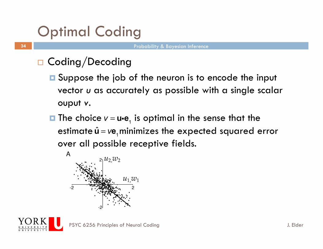
34
Optimal Coding
Coding/Decoding Suppose the job of the neuron is to encode the input
vector u as accurately as possible with a single scalar ouput v.
The choice is optimal in the sense that the estimate minimizes the expected squared error over all possible receptive fields.
v = uie1
u = ve1

Probability & Bayesian Inference
J. Elder PSYC 6256 Principles of Neural Coding
35
Information Theory
Projection of the input onto the first principal component of the input correlation matrix maximizes the variance of the output.
For a Gaussian input, this also maximizes the output entropy.
If the output is corrupted by Gaussian noise, this also maximizes the information the output v carries about the input u.
v = uie1
Multiple Postsynaptic Neurons
Probability & Bayesian Inference
J. Elder PSYC 6256 Principles of Neural Coding
37
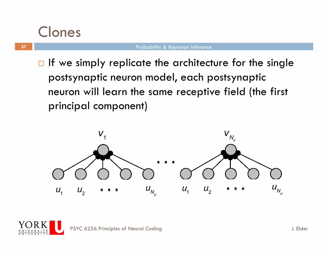
Clones
If we simply replicate the architecture for the single postsynaptic neuron model, each postsynaptic neuron will learn the same receptive field (the first principal component)
v1 vNv
u1 u2 uNµ u1 u2
uNµ

Probability & Bayesian Inference
J. Elder PSYC 6256 Principles of Neural Coding
38
Competition Between Output Neurons
In order to achieve diversity, we must incorporate some form of competition between output neurons.
The basic idea is for each output neuron to inhibit the others when it is responding well. In this way it ‘takes ownership’ of certain inputs.
This leads to diversification in receptive fields. This inhibition is achieved through recurrent
connections between output neurons
Probability & Bayesian Inference
J. Elder PSYC 6256 Principles of Neural Coding
39
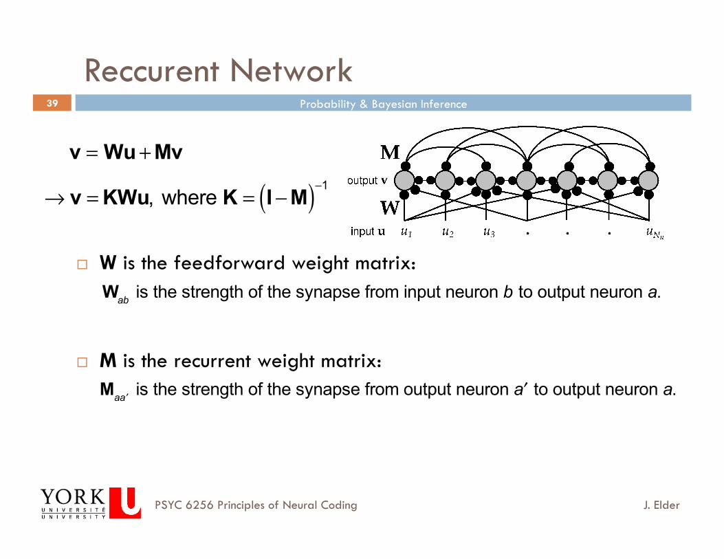
Reccurent Network
W is the feedforward weight matrix:
M is the recurrent weight matrix:
v = Wu+Mv
Wab is the strength of the synapse from input neuron b to output neuron a.
Ma ′a is the strength of the synapse from output neuron ′a to output neuron a.
→ v = KWu, where K = I−M( )−1
Probability & Bayesian Inference
J. Elder PSYC 6256 Principles of Neural Coding
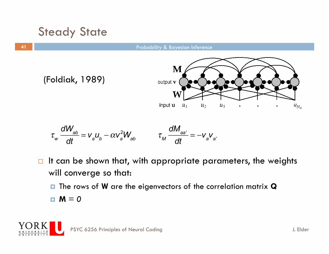
40
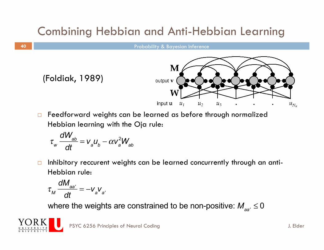
Combining Hebbian and Anti-Hebbian Learning
Feedforward weights can be learned as before through normalized Hebbian learning with the Oja rule:
Inhibitory reccurent weights can be learned concurrently through an anti-Hebbian rule:
τw
dWab
dt= vaub −αva
2Wab
τM
dMa ′a
dt= −vav ′a
where the weights are constrained to be non-positive: Ma ′a ≤ 0
(Foldiak, 1989)
Probability & Bayesian Inference
J. Elder PSYC 6256 Principles of Neural Coding
41
Steady State
It can be shown that, with appropriate parameters, the weights will converge so that: The rows of W are the eigenvectors of the correlation matrix Q
M = 0
τw
dWab
dt= vaub −αva
2Wab τM
dMa ′a
dt= −vav ′a
(Foldiak, 1989)
Probability & Bayesian Inference
J. Elder PSYC 6256 Principles of Neural Coding
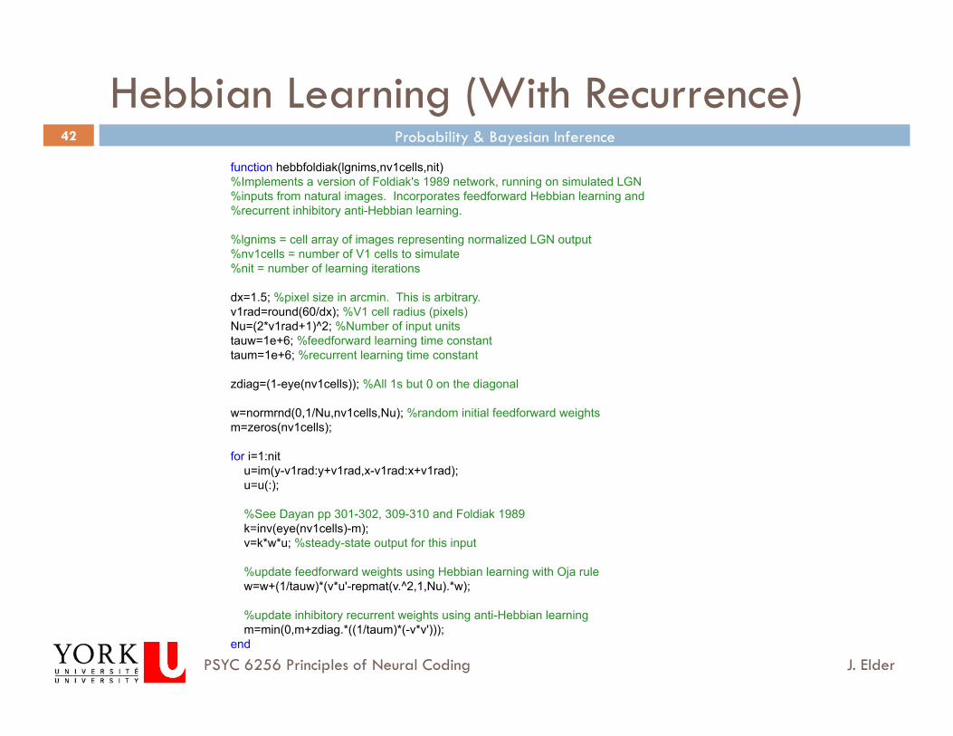
42
Hebbian Learning (With Recurrence) function hebbfoldiak(lgnims,nv1cells,nit) %Implements a version of Foldiak's 1989 network, running on simulated LGN %inputs from natural images. Incorporates feedforward Hebbian learning and %recurrent inhibitory anti-Hebbian learning.
%lgnims = cell array of images representing normalized LGN output %nv1cells = number of V1 cells to simulate %nit = number of learning iterations
dx=1.5; %pixel size in arcmin. This is arbitrary. v1rad=round(60/dx); %V1 cell radius (pixels) Nu=(2*v1rad+1)^2; %Number of input units tauw=1e+6; %feedforward learning time constant taum=1e+6; %recurrent learning time constant
zdiag=(1-eye(nv1cells)); %All 1s but 0 on the diagonal
w=normrnd(0,1/Nu,nv1cells,Nu); %random initial feedforward weights m=zeros(nv1cells);
for i=1:nit u=im(y-v1rad:y+v1rad,x-v1rad:x+v1rad); u=u(:);
%See Dayan pp 301-302, 309-310 and Foldiak 1989 k=inv(eye(nv1cells)-m); v=k*w*u; %steady-state output for this input
%update feedforward weights using Hebbian learning with Oja rule w=w+(1/tauw)*(v*u'-repmat(v.^2,1,Nu).*w);
%update inhibitory recurrent weights using anti-Hebbian learning m=min(0,m+zdiag.*((1/taum)*(-v*v'))); end

Probability & Bayesian Inference
J. Elder PSYC 6256 Principles of Neural Coding
43
Output
20 40 60 80
20
40
60
8020 40 60 80
20
40
60
80
20 40 60 80
20
40
60
8020 40 60 80
20
40
60
80
0 1000 2000 3000 4000 5000 6000 7000 8000 9000 100000
0.5
1
1.5
2
Norm(w)
0 1000 2000 3000 4000 5000 6000 7000 8000 9000 100000
0.5
1
1.5
Norm(m)


