29
1 Daniel Felsenstein Eyal Ashbel Simultaneous Modeling of Developer Behavior and Land Prices in UrbanSim UrbanSim European Users Group meeting, ETH Zurich, 17-18 th March 2008
| Date post: | 19-Dec-2015 |
| Category: |
Documents |
| View: | 215 times |
| Download: | 0 times |

1
Daniel Felsenstein
Eyal Ashbel
Simultaneous Modeling of Developer Behavior and Land Prices in UrbanSim
Simultaneous Modeling of Developer Behavior and Land Prices in UrbanSim
UrbanSim European Users Group meeting, ETH Zurich, 17-18th March 2008

2
The Motivation
The Motivation
• In UrbanSim, interdependence between developer behavior and land prices is noted.
• Interdependence between dev.behav/land prices and h’hold and job location choice, is also noted.
• However, in the model developer behavior and land prices are modeled independently.
• In practice, the two occur simultaneously

3
Motivation cont.
Motivation cont.
• UrbanSim models assumes prices are exogenous to interaction between buyers and sellers (their individual transactions are too small to affect aggregate prices).
• But much urban economics points to endogeneity issue: developer behavior depends on land prices and land prices depend on developer behavior
• Issue of endogeneity means dealing with:
– Correct identification of models (error structures)
– Instrumentation
– Dynamics

4
Motivation cont 2.
Motivation cont 2.
• Dynamics in current land price model: cross-section simulation of end-of-the-year-prices based on updated cell characteristics (from developer model, h’hold and jobs location choices and transport model).
• These land prices then influence h’holds, jobs, developer behavior in next year: back-door endogeneity?
• Prices also fixed by expectations of price (rational expectations world)

5
TheoryTheory
Relative PriceRelative Price QuantityQuantity
itB
A
it
it
P
P L
LA
B
A
P
P
L
LA
AB
D
S' (π+1= π)
S'' (π+1> π)

6
SupplySupply
itite1ititiit UλZγπβπασ
itititit VXπd
Z, X = vectors of variables that cause supply/demand curves to shift
general price is sum of parcel prices.
n
1iitittit w;θ
itit d
(–)
(+)DemandDemand
Equilibrium
Equilibrium
7
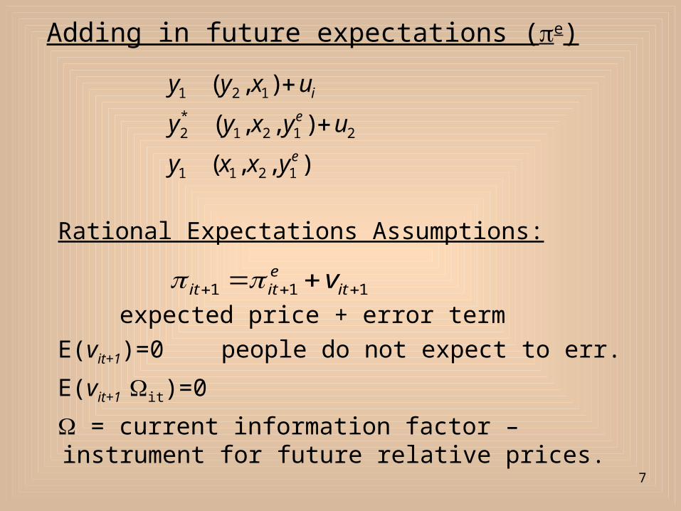
Rational Expectations Assumptions:
expected price + error termE(vit+1)=0 people do not expect to err.
E(vit+1 it)=0
= current information factor – instrument for future relative prices.
Adding in future expectations (e)
),,(
),,(
),(
1211
2121*2
121
e
e
i
yxxy
uyxyy
uxyy
111 iteitit v

8
Adding time factor to future expectations:
yt=xt+[yt+1-vt+1]+ut E(vt+1,ut)=0
=xt+yt+1+ut- vt+1 E(yet+1)<0
IV: yt+1 , xt , vt+1
1te
1t1t
te
1ttt
vyy
uyxy

9
Estimation StrategyEstimation Strategy
Maddala (1983): simultaneous equationsUse probit two-stage least squares (P2SLS)CDSIMEQ routine (STATA Journal 2003)
111
*211 uyy X
22212*2 uyy X
Land price model (OLS)
Developer model (probit)

10
1. Simultaneous equations
2. y*2 is not observed,
rewrite (1) and (2) as
3. Estimate reduced form
4. Extract predicted values
5. Plug-in fitted values and adjust covariance matrix
)2(
)1(
22212*2
111*211
uyy
uyy
X
X
)4(
)3(
2
22
2
21
2
2**2
111**
2211
u
yy
uyy
X
X
)6(
)5(
222**
2
1111
vy
vy
X
X
)8(ˆˆ
)7(ˆˆ
2**
2
11
X
X
y
y
)10(ˆ
)9(ˆ
22212**
2
111**
211
uyy
uyy
X
X
11
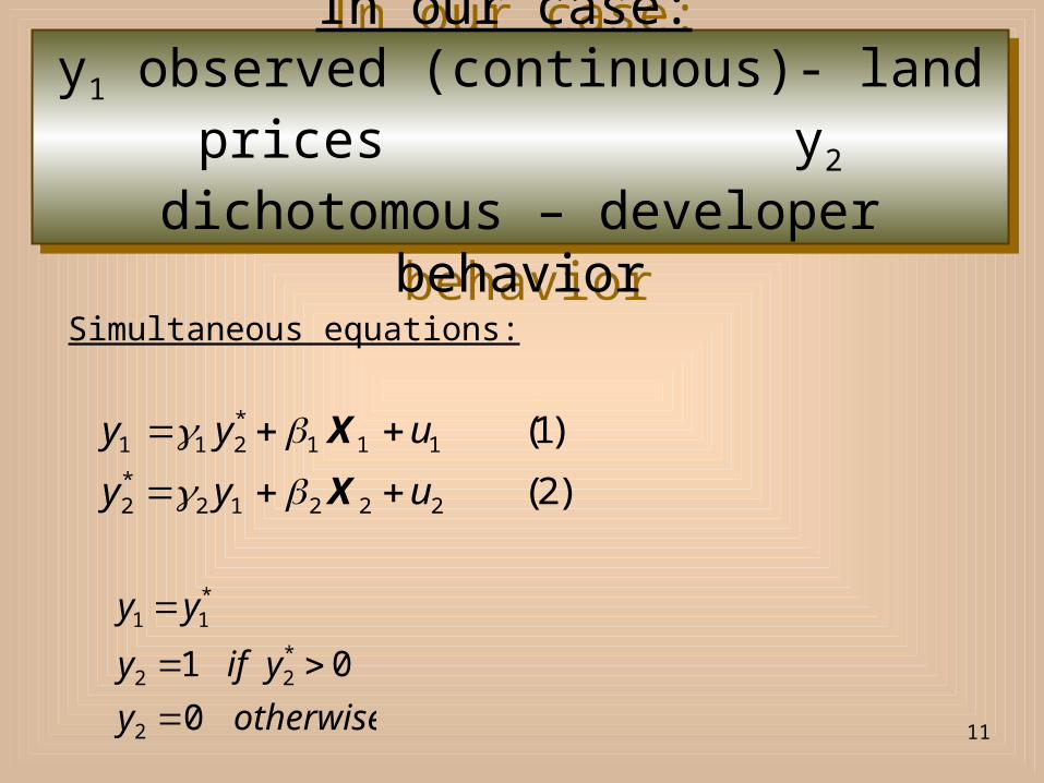
In our case: y1 observed (continuous)- land prices y2 dichotomous –
developer behavior
In our case: y1 observed (continuous)- land prices y2 dichotomous –
developer behavior
otherwisey
yify
yy
0
01
2
*22
*11
)2(
)1(
22212*2
111*211
uyy
uyy
X
X
Simultaneous equations:

12
As is not observed (ie only observed as a dichotomous variable), equations (1) and (2) are re-written:
*2y
)4(
)3(
2
22
2
21
2
2**2
111**
2211
u
yy
uyy
X
X
This has implications for standard errors that will need to be corrected later on.

13
Stage 1: (estimated by OLS and probit): models fitted using all exogenous variables. Predicted values obtained.
)6(
)5(
222**
2
1111
vy
vy
X
X
)8(ˆˆ
)7(ˆˆ
2**
2
11
X
X
y
y
From these reduced-form estimates, predicted values from each model are obtained for use in Stage 2.
Two-stage Estimation Two-stage Estimation
X= matrix of all exogenous variables
Π1’Π2,= vectors of parameters to be estimated

14
Two-stage Estimation cont.
Two-stage Estimation cont.
Stage 2: (estimated by OLS and probit): original endogenous variables in (3) and (4) are replaced by their fitted values from (7) and (8).
1**
2 ˆ,ˆ yy
Finally, need correction for standard errors (adjustment of the variance- covariance matrix) as models based on
and not on the appropriate
)10(ˆ
)9(ˆ
22212**
2
111**
211
uyy
uyy
X
X
1**
2 , yy

15
Estimated Results - Example
Estimated Results - Example
Land PricesDeveloper Behavior 2 -(-1), Residential – no
further developmentConstant 12.43**
Developer Behavior 0.541*
Travel time CBD -0.00253**
Percent water -0.00710 **
ln resid. units walking dist -0.0808**
ln resid. units 0.104**
ln distance highway 0.0468**
ln commercial sq. ft. 0.0199**
Mixed Use 1.477**
Residential -2.377 **
Constant 4.113*
ln land prices -0.1300Access to arterial hwy. -0.5499*
Recent transitions to resid. (walking dist) -0.58853Recent transitions to same type (walking dist) -1.4915**
Percent mixed use (walking dist) 0.5465*
Percent same type cells (walking dist)0.01518*
ln resid. units -0.8261**
-2log likelihood -N 2,919R2 0.73LR X2 -
-57.634238
-
214.5(p<0.000)

16
Tel Aviv Metropolitan Area
Tel Aviv Metropolitan Area
• 1,683 sq km. • Three million
inhabitants.• One million employees• 49 % National GNP.• 60 local authorities
(city governments)
17
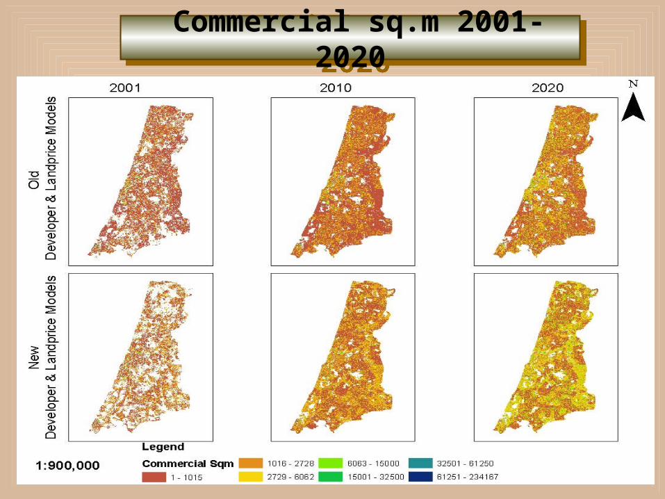
Commercial sq.m 2001-2020
Commercial sq.m 2001-2020

18
Non- residential land values, 2001-2020
Non- residential land values, 2001-2020

19
Non-residentialNon-residential
• Non-resid sq m: development starts later but reaches more extreme values
• Similar trends to individual model estimation. Accentuated suburban non-residential development
• Simultaneous estimation makes for more extreme values in non- resid land prices. Less smooth price gradient

20
Density – persons per grid cell, 2001-2020
Density – persons per grid cell, 2001-2020

21
Residential Land Values, 2001-2020
Residential Land Values, 2001-2020
22
ResidentialResidential
• Simultaneous estimation predicts more population deconcentration.
• Residential land values are estimated to be higher in suburban locations than in CBD (using simultaneous estimation)
• Individual estimation gives opposite picture: higher residential prices closer to CBD

23
Local Authorities within the Metro Area
Local Authorities within the Metro Area

24
City Name Delta 2001 Delta 2010 Delta 2020 Delta 2001 Delta 2010 Delta 2020Ra'anana 17% 0% 1% 4% 1% 5%Petah Tikva -3% 11% -2% 1% 1% 2%Netanya 5% 2% -4% 1% 2% 1%Rehovot 0% 9% 2% 1% -1% 2%Rishon Leziyon -6% 17% 2% 1% 0% 1%Ashdod 2% 8% 10% 3% 1% 2%Tel Aviv 5% 5% 1% 2% 3% 1%
Average Income Households
Delta=(new-old)/new
Households Data

25
Grid Cells Data
City Name Delta 2001 Delta 2010 Delta 2020Ra'anana -22% -4% 0%Petah Tikva 21% 28% 30%Netanya 3% 15% 17%Rehovot 27% 27% 27%Rishon Leziyon 20% 31% 34%Ashdod 24% 34% 40%Tel Aviv 8% 14% 13%
Commercial Sqm
26
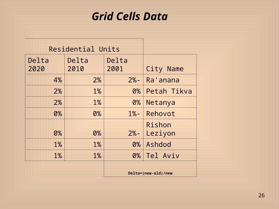
Grid Cells Data
Residential Units
City NameDelta 2001
Delta 2010
Delta 2020
Ra'anana-2%2%4%Petah Tikva0%1%2%Netanya0%1%2%Rehovot-1%0%0%Rishon Leziyon-2%0%0%Ashdod0%1%1%Tel Aviv0%1%1%
Delta=(new-old)/new

27
Grid Cells Data
Fraction Residential
City NameDelta 2001
Delta 2010
Delta 2020
Ra'anana-30%5%5%Petah Tikva-10%5%5%Netanya-7%2%2%Rehovot-20%-2%-2%Rishon Leziyon-23%-1%-2%Ashdod-9%-3%-4%Tel Aviv0%1%1%
Delta=(new-old)/new

28
Results for Individual Local Authorities
Results for Individual Local Authorities
• Results tend to stabilize over the longer term (2020)
• Households data: simultaneous estimation generally yields higher outcomes (positive deltas) than individual estimation.
• Changes in attributes of cells: estimates of changes in non-residential cells (units, area) much more volatile than for residential cells. Confirms results relating to land values.
• Southern local authorities estimated gains much more in non-residential units than in residential (implications for fiscal independence).

29
ConclusionsConclusions
• Avoiding endogeneity in price fixing= the easy way out?
• Explicit treatment of prices in UrbanSim- can this be improved? (Prices respond at the end of the year to grid cell characteristics of location, balance of supply an demand at each location)
• Price expectations need to be included (need credible instrument)
• Is this more suited to UrbanSim4?


