1 Energy Efficient Broadcasting Using Sparse Topology in Wireless Ad Hoc Networks Kousha Moaveninejad ? Xiang-Yang Li ? Keywords —Wireless ad hoc networks, broadcasting, power consumption, spare structures, topology control. I. Introduction Wireless Ad Hoc Networks: Due to its potential applica- tions in various situations such as battlefield, emergency relief, environment monitoring, and so on, wireless ad hoc networks [1], [2], [3], [4] have recently emerged as a pre- mier research topic. Wireless networks consist of a set of wireless nodes which are spread over a geographical area. These nodes are able to perform processing as well as ca- pable of communicating with each other by means of a wireless ad hoc network. With coordination among these wireless nodes, the network together will achieve a larger task both in urban environments and in inhospitable ter- rain. For example, the sheer numbers of wireless sensors and the expected dynamics in these environments present unique challenges in the design of wireless sensor networks. Many excellent researches have been conducted to study problems in this new field [1], [2], [5], [3], [6], [4]. In this paper, we consider a wireless ad hoc network consisting of a set V of n wireless nodes distributed in a two-dimensional plane. Each wireless node has an omni- directional antenna. This is attractive because a single transmission of a node can be received by many nodes within its vicinity which, we assume, is a disk centered at the node. This property is also known as ”wireless mul- ticast advantage ”. We call the radius of this disk the trans- mission range of this wireless node. In other words, node v can receive the signal from node u if node v is within the transmission range of the sender u. Otherwise, two nodes communicate through multi-hop wireless links by using in- termediate nodes to relay the message. Consequently, each node in the wireless network also acts as a router, forward- ing data packets for other nodes. By a proper scaling, we assume that all nodes have the maximum transmission range equal to one unit. These wireless nodes define a unit disk graph UDG(V ) in which there is an edge between two nodes if and only if their Euclidean distance is less than or equal to one. In addition, we assume that each node has a low-power Global Position System (GPS) receiver, which provides the position information of the node itself. If GPS is not avail- able, the distance between neighboring nodes can be esti- mated on the basis of incoming signal strengths. Relative co-ordinates of neighboring nodes can be obtained by ex- ? Department of Computer Science, Illinois Institute of Technology, 10 W. 31st Street, Chicago, IL 60616, USA. Email [email protected], [email protected]. changing such information between neighbors [7]. With the position information, we can apply computational ge- ometry techniques to solve some challenging questions in wireless networks. Power-Attenuation Model: Energy conservation is a criti- cal issue in wireless network for the node and network life, since the nodes are powered by batteries only. Each wire- less node typically has a portable set with transmission and reception processing capabilities. To transmit a sig- nal from a node to the other node, the power consumed by these two nodes consists of the following three parts. First, the source node needs to consume some power to prepare the signal. Second, in the most common power- attenuation model, the power needed to support a link uv is kuvk β , where kuvk is the Euclidean distance between u and v, β is a real constant between 2 and 5 dependent on the transmission environment. This power consumption is typically called path loss. Finally, when a node receives the signal, it needs to consume some power to receive, store and then process that signal. For simplicity, this overhead cost can be integrated into one cost, which is almost the same for all nodes. Thus, we will use c to denote such con- stant overhead. In most results surveyed here, it is assumed that c = 0, i.e., the path loss is the major part of power consumption to transmit signals. The power cost p(e) of a link e = uv is then defined as the power consumed for transmitting signal from u to node v, i.e. p(uv)= kuvk β . Broadcast, Multicast and Unicast: Broadcasting is a com- munication paradigm that allows sending data packets from a source node to all nodes in the network, Multi- casting is a communication paradigm that allows sending data packets from a source node to multiple receivers and Unicasting is a communication paradigm that allows send- ing data packets from a source node to a single destination node. In one-to-all model, (using omni-directional anten- nas) transmission by each node can reach all nodes that are within radius distance from it, while in the one-to-one model, each transmission is directed toward only one neigh- bor (using, for instance, directional antennas or separate frequencies for each node). The broadcasting in liter- ature has been studied mainly for one-to-all model and we will use that model in this chapter. Broad- casting is also frequently referred to as flooding. Broadcasting and multicasting in wireless ad hoc net- works are critical mechanisms in various applications such as information diffusion, wireless networks, and also for maintaining consistent global network information. Broad- casting is often necessary in MANET routing protocols. For example, many unicast routing protocols such as Dy- namic Source Routing (DSR), Ad Hoc On Demand Dis-
Transcript
1
Energy Efficient Broadcasting Using SparseTopology in Wireless Ad Hoc Networks
Kousha Moaveninejad? Xiang-Yang Li?
Keywords—Wireless ad hoc networks, broadcasting, powerconsumption, spare structures, topology control.
I. Introduction
Wireless Ad Hoc Networks: Due to its potential applica-tions in various situations such as battlefield, emergencyrelief, environment monitoring, and so on, wireless ad hocnetworks [1], [2], [3], [4] have recently emerged as a pre-mier research topic. Wireless networks consist of a set ofwireless nodes which are spread over a geographical area.These nodes are able to perform processing as well as ca-pable of communicating with each other by means of awireless ad hoc network. With coordination among thesewireless nodes, the network together will achieve a largertask both in urban environments and in inhospitable ter-rain. For example, the sheer numbers of wireless sensorsand the expected dynamics in these environments presentunique challenges in the design of wireless sensor networks.Many excellent researches have been conducted to studyproblems in this new field [1], [2], [5], [3], [6], [4].
In this paper, we consider a wireless ad hoc networkconsisting of a set V of n wireless nodes distributed in atwo-dimensional plane. Each wireless node has an omni-directional antenna. This is attractive because a singletransmission of a node can be received by many nodeswithin its vicinity which, we assume, is a disk centeredat the node. This property is also known as ”wireless mul-ticast advantage”. We call the radius of this disk the trans-mission range of this wireless node. In other words, nodev can receive the signal from node u if node v is within thetransmission range of the sender u. Otherwise, two nodescommunicate through multi-hop wireless links by using in-termediate nodes to relay the message. Consequently, eachnode in the wireless network also acts as a router, forward-ing data packets for other nodes. By a proper scaling,we assume that all nodes have the maximum transmissionrange equal to one unit. These wireless nodes define a unitdisk graph UDG(V ) in which there is an edge between twonodes if and only if their Euclidean distance is less than orequal to one.
In addition, we assume that each node has a low-powerGlobal Position System (GPS) receiver, which provides theposition information of the node itself. If GPS is not avail-able, the distance between neighboring nodes can be esti-mated on the basis of incoming signal strengths. Relativeco-ordinates of neighboring nodes can be obtained by ex-
?Department of Computer Science, Illinois Institute of Technology,10 W. 31st Street, Chicago, IL 60616, USA. Email [email protected],[email protected].
changing such information between neighbors [7]. Withthe position information, we can apply computational ge-ometry techniques to solve some challenging questions inwireless networks.
Power-Attenuation Model: Energy conservation is a criti-cal issue in wireless network for the node and network life,since the nodes are powered by batteries only. Each wire-less node typically has a portable set with transmissionand reception processing capabilities. To transmit a sig-nal from a node to the other node, the power consumedby these two nodes consists of the following three parts.First, the source node needs to consume some power toprepare the signal. Second, in the most common power-attenuation model, the power needed to support a link uvis ‖uv‖β , where ‖uv‖ is the Euclidean distance betweenu and v, β is a real constant between 2 and 5 dependenton the transmission environment. This power consumptionis typically called path loss. Finally, when a node receivesthe signal, it needs to consume some power to receive, storeand then process that signal. For simplicity, this overheadcost can be integrated into one cost, which is almost thesame for all nodes. Thus, we will use c to denote such con-stant overhead. In most results surveyed here, it is assumedthat c = 0, i.e., the path loss is the major part of powerconsumption to transmit signals. The power cost p(e) ofa link e = uv is then defined as the power consumed fortransmitting signal from u to node v, i.e. p(uv) = ‖uv‖β .
Broadcast, Multicast and Unicast: Broadcasting is a com-munication paradigm that allows sending data packetsfrom a source node to all nodes in the network, Multi-casting is a communication paradigm that allows sendingdata packets from a source node to multiple receivers andUnicasting is a communication paradigm that allows send-ing data packets from a source node to a single destinationnode. In one-to-all model, (using omni-directional anten-nas) transmission by each node can reach all nodes thatare within radius distance from it, while in the one-to-onemodel, each transmission is directed toward only one neigh-bor (using, for instance, directional antennas or separatefrequencies for each node). The broadcasting in liter-ature has been studied mainly for one-to-all modeland we will use that model in this chapter. Broad-casting is also frequently referred to as flooding.
Broadcasting and multicasting in wireless ad hoc net-works are critical mechanisms in various applications suchas information diffusion, wireless networks, and also formaintaining consistent global network information. Broad-casting is often necessary in MANET routing protocols.For example, many unicast routing protocols such as Dy-namic Source Routing (DSR), Ad Hoc On Demand Dis-
2
tance Vector (AODV), Zone Routing Protocol (ZRP), andLocation Aided Routing (LAR) use broadcasting or aderivation of it to establish routes.
Currently, most of the protocols rely on a simplistic formof broadcasting called Flooding, in which each node (or allnodes in a localized area) retransmits each received uniquepacket exactly one time. The main problems with Floodingare that it typically causes unproductive and often harm-ful bandwidth congestion, as well as inefficient use of noderesources. Broadcasting is also more efficient than send-ing multiple copies of the same packet through unicast. Itis highly important to use power-efficient broadcast algo-rithms for such networks since, as mentioned before,wireless devises are often powered by batteries only.
Recently, a number of research groups have proposedmore efficient broadcasting techniques [8], [9], [10], [11],[12], [13], [14] with various goals such as minimizing thenumber of retransmissions, minimizing the total powerused by all transmitting nodes, minimizing the overall de-lay of the broadcasting, and so on. Williams and Camp[13] classified the broadcast protocols into four categories:simple (blind) flooding, probability based, area based, andneighbor knowledge methods. Wu and Lou [15] classifiedbroadcasting protocols based on neighbor knowledge infor-mation into four categories: global, quasi-global, quasi-local, and local. The global broadcast protocol, whichcould be centralized or distributed, is based on globalstate information. In quasi-global broadcasting, a broad-cast protocol is based on partial global state information.For example, the approximation algorithm in [16] is basedon building a global spanning tree (a form of partial globalstate information) that is constructed in a sequence of se-quential propagations. In quasi-local broadcasting, a dis-tributed broadcast protocol is based on mainly local stateinformation and occasionally partial global state informa-tion. Cluster networks are such examples: while clusterscan be constructed locally for most of the time, the chainreaction does occur occasionally. In local broadcasting, adistributed broadcast protocol is solely based on local stateinformation. All protocols that select forward nodes locally(based on 1-hop or 2-hop neighbor set) belong to this cat-egory. It has been recognized that scalability in wirelessnetworks cannot be achieved by relying on solutions whereeach node requires global knowledge about the network.To achieve scalability, the concept of localized algorithmswas proposed, as distributed algorithms where simple localnode behavior, based on local knowledge, achieves a desiredglobal objective.
MAC Specification: Collision avoidance is inherently dif-ficult in MANETs; one often cited difficulty is overcom-ing the hidden node problem, where a node cannot decidewhether some of its neighbors are busy receiving transmis-sions from an uncommon neighbor. The 802.11 MAC fol-lows a Carrier Sense Multiple Access/Collision Avoidance(CSMA/CA) scheme. For unicasting, it utilizes a RequestTo Send (RTS) / Clear To Send (CTS) / Data / Acknowl-edgment (ACK) procedure to account for the hidden nodeproblem. However, the RTS/CTS/Data/ACK procedure is
too cumbersome to implement for broadcast packets as itwould be difficult to coordinate and bandwidth expensive:a relay node has to perform RTS/CTS individually withall its neighbors that should receive the packets. Thus,the only requirement made for broadcasting nodes is thatthey assess a clear channel before broadcasting. Unfor-tunately, clear channel assessment does not prevent colli-sions from hidden nodes. Additionally, no resource is pro-vided for collision when two neighbors assess a clear chan-nel and transmit simultaneously. Ramifications of this en-vironment are subtle but significant. Unless specific meansare implemented at the network layer, a node has no wayof knowing whether a packet was successfully reached byits neighbors. In congested networks, a significant amountof collisions occur leading to many dropped packets. Themost effective broadcasting protocols try to limit the prob-ability of collisions by limiting the number of rebroadcastsin the network. Thus, it is often imperative the underly-ing structure for broadcasting is degree bounded and thelinks are at similar lengths. By using a power adjustmentat each node, the collision of packets and contention forchannel will be alleviated. Notice that, if the underlyingstructure for broadcasting is degree bounded, we can eitheruse RTS/CTS scheme to avoid hidden node problem, or wecan rebroadcast the dropped packets (such rebroadcast willbe less since the number of intended receiving neighbors isbounded by a small constant).
Performance Measurement: The performance of broad-cast protocols can be measured by variety of metrics. Acommonly used metric is the number of message retrans-missions with respect to the number of nodes. In caseof broadcasting with adjustable transmission power, whichwill be explained later in section II, the total power is usedas performance metrics, while In case of broadcasting withnon-adjustable transmission power, which also will be ex-plained later in section II, the number of forwarding nodes,also known as dominators, is used as performance metrics
Organization The rest of the chapter is organized as fol-lows. In Section II, we review the priori arts of energyefficient broadcasting based on structures constructed incentralized manner or localized manner. In Section III westudy broadcasting based on sparse topology constructedlocally and to validate our theoretical results we conductedextensive simulations in Section III. We conclude the paperin Section VI.
II. Preliminaries
Network Model: We assume that all wireless nodesare given as a set V of n points in a two dimensional spaceand each wireless node has some computational power andan omni-directional antenna. This is attractive because asingle transmission by a wireless node can be received byall wireless nodes within its vicinity. It is also assumedthat the nodes are almost static in a reasonable period oftime, all wireless nodes have distinctive identities and eachwireless node u has a maximum transmission range Ru. Adirected communication graph
−→G = (V,
−→E ) over a set V
of wireless nodes has an edge −→uv from node u to node v
3
if and only if node u can send message directly to node v(i.e., ‖uv‖ ≤ Ru). If the maximum transmission range ofall wireless nodes are the same, then all communicationsedge will be mutual, i.e., −→uv exists iff −→vu exists, and we canignore the direction of edges and by proper scaling we canset the maximum transmission of all wireless nodes to oneunit and model the graph as UDG(Unit Disk Graph).UnitDisk Graph is an undirected graph where there is an edgebetween two nodes if and only if the Euclidean distancebetween them is less than one unit (See Figure 1(a) for anillustration). We always assume the network is connected,otherwise sending message from the source node to all thenodes in the network would be impossible.
Minimum Connected Dominating Set:A subset Sof V is a dominating set if each node u in V is either inS or is adjacent to some node v in S. Nodes from S arecalled dominators, while nodes not is S are called dom-inatees. A subset C of V is a connected dominating set(CDS) if C is a dominating set and C induces a connectedsubgraph. Consequently, the nodes in C can communicatewith each other without using nodes in V − C. A dom-inating set with minimum cardinality is called minimumdominating set, denoted by MDS. A connected dominatingset with minimum cardinality is denoted by minimum con-nected dominating set (MCDS). A broadcasting based onconnected dominating set only uses the nodes in CDS torelay the message.
In Figure 1 dominators are shown by squares. Figure1(a) shows the original UDG graph and as can be seen inFigure 1(b), all nodes in the graph are either in the back-bone or at least have a neighbor in the backbone. Figure1(c) shows the backbone of the same graph.
Broadcast Tree: Any broadcast routing can be viewedas an arborescence (a directed tree) T , rooted at the sourcenode of the broadcasting, that spans all nodes. Let fT (p)denote the transmission power of the node p required byT . For any leaf node p of T , fT (p) = 0. For any internalnode p of T , fT (p) depends on the power model that isused for broadcasting.
In Figure 2(a) a message from source node s is broad-casted to all nodes in the network. Dashed circles repre-sent the transmission area of node s,1 and 2. Figure 2(b)shows an isomorphic arborescence to what is shown in Fig-ure 2(a). As can be seen leaf nodes, (i.e., nodes 2, 3, 4, 6, 7,and 8 in this examples) do not contribute in broadcast andconsume no energy.
Power Model:In the literature, there are two commonenergy models that could be used for broadcasting:• Non-adjustable power : In this model, each node uses itsmaximum transmission range to send message or data tothe nodes in its vicinity. In other words, the power con-sumed at each node is not adjustable and is a constant forall relay nodes. Since we assumed the maximum transmis-sion range of all nodes is 1 unit, for any internal node p inthe broadcast tree T we have:
fT (p) = 1,
So minimizing the total power used by a reliable broadcast
tree is equivalent to the minimum connected dominatingset problem (MCDS) (i.e., minimize the number of nodesthat relay the message), since all relaying nodes of a reliablebroadcast form a connected dominating set (CDS).• Adjustable power : In this model the power consumed ateach node is adjustable. we assume that the power con-sumed by a relay node u is ‖uv‖β , where the real numberβ ∈ [2, 5] depending on transmission environment and v isthe farthest neighbor of u in the broadcast tree. For anyinternal node p of T ,
fT (p) = maxpq∈T
‖pq‖β,
in other words, the β-th power of the longest distance be-tween p and its children in T . The total energy requiredby T is
∑p∈P fT (p).
In the rest of this chapter, for these two energy models re-spectively, we will review several methods that can buildsome broadcast trees whose energy consumption are withina constant factor of the optimum if the original communi-cation graph is modelled by unit disk graph.
Approximation ratio: Approximation ratio of aheuristic of a minimization problem is the maximum ra-tio of value given by the heuristic to value of the answer ofthe problem. So for minimization problem A, and heuristicH, Approximation ratio α is defined as:
α =SUPA(H)
A(optimal)
and Approximation ratio of a heuristic of a maximizationproblem is the maximum ratio of the value of the optimalanswer of the problem to the value given by the heuristic.Sofor maximization problem A, and heuristic H, Approxima-tion ratio α is defined as:
α =SUPA(optimal)
A(H)
A. Centralized Methods
A.1 Based on adjustable power model:MST and Variations
Some centralized methods are based on greedy heuris-tics. Three greedy heuristics were proposed in [17] for theminimum-energy broadcast routing problem: MST (min-imum spanning tree), SPT (shortest-path tree), and BIP(broadcasting incremental power). MST is the tree thatspans all the nodes and has the minimum total edge length.The MST heuristic first applies the Prim’s algorithm to ob-tain a MST, and then orients it as an arborescence rootedat the source node. SPT is the tree that spans all thenodes such that the shortest path between every pair ofnodes is included. In other words, for any pairs of nodesu and v, the shortest Euclidean path that connects node uto node v belongs to SPT. The SPT heuristic applies theDijkstra’s algorithm to obtain a SPT rooted at the sourcenode. The BIP heuristic is the node version of Dijkstra’salgorithm for SPT. It maintains, throughout its execution,a single arborescence rooted at the source node. The ar-borescence starts from the source node, and new nodes are
4
(a) (b) (c)Fig. 1. UDG and CDS example.
8
1
2
3
4
5 7
6
S
8
15
67
S
2 3 4
(a) (b)Fig. 2. Broadcast tree example.
added to the arborescence one at a time on the minimumincremental cost basis until all nodes are included in thearborescence. The incremental cost of adding a new nodeto the arborescence is the minimum additional power in-creased by some node in the current arborescence to reachthis new node.
The minimum-energy broadcast routing problem is dif-ferent from the conventional link-based minimum spanningtree (MST) problem. Minimum-energy broadcast rout-ing problem finds the tree such that the total power con-sumed by the node in the broadcast tree in minimized whilethe conventional link-based minimum spanning tree (MST)problem finds the tree such that the total Euclidean edgelength is minimized.
Indeed, while the MST can be solved in polynomial timeby algorithms such as Prim’s algorithm and Kruskal’s al-gorithm [18], the minimum-energy broadcast routing prob-lem cannot be solved in polynomial time unless P=NP [19].Recently, Clementi et al. [19] proved that the minimum-energy broadcast routing problem is NP-hard and obtaineda parallel but weaker result to those of [20].
Wan et al. [20] showed that the approximation ratios ofMST and BIP are between 6 and 12 and between 13
3 and12 respectively.
here approximation ratio of a heuristic is the maximumratio of the energy needed to broadcast a message based
on the arborescence generated by this heuristic to the leastnecessary energy by any arborescence for any set of points.
Another two greedy heuristics were proposed in [17] forthe minimum-energy broadcast routing problem: BLU andBLiMST. BLU (Broadcast Least-Unicast-cost) algorithm isa straightforward (but far from optimal) approach. BLUbuilds the broadcast trees that consist of the superposi-tion of the best unicast paths to each individual destina-tion. It is assumed that an underlying unicast algorithm(such as the Bellman-Ford or Dijkstra algorithm) provides”minimum-distance” paths from the source node to everyother node. Since BLU is based on the use of a scalableunicast algorithm, it also is scalable.
Also note that, although algorithms based onminimum distance paths are normally used forpacket-switched applications, this approach is beingused here for session oriented traffic, since a cost(involving power and possibly congestion) can bedefined for each link in the network. By contrast,in circuit-switched wired applications it is difficultto define a link cost because energy is not of con-cern and because delay is not an appropriate met-ric (as it would be in packet-switched applications)since resources are reserved in circuit-switched ap-plications. Instead, blocking probability is the onlyoverall objective, and there is no known way of
5
mapping that objective to individual link metrics.Summarizing the above, we have:BLU: A minimum-cost path from the source node to ev-
ery other node is established. The broadcast tree consistsof the superposition of these unicast paths.
The failure of BLU to exploit the wireless multicast ad-vantage results in higher overall power expenditure.
BLiMST (Broadcast Link-based MST) based on the useof the standard MST formulation (as in wired networks)in which a link cost is associated with each pair of nodes(i.e., the power to sustain the link). Thus, the ”wirelessmulticast advantage” is ignored in the construction of theMST. Since the MST problem is of polynomial complexity,it is scalable. Once the MST is constructed in this manner,the evaluation of its cost (i.e., the total power needed tosustain the broadcast tree) does take into consideration thewireless multicast advantage.
Summarizing the above, we have:BLiMST: A minimum-cost (minimum-power) spanning
tree is formed using standard (link-based) MST techniques.Similar to the case of BLU, the failure of BLiMST to
exploit the wireless multicast advantage results in higheroverall power expenditure. The complexity of BLU, whenimplemented by means of the Dijkstra algorithm, is O(N2),where N is the number of nodes in the network. Thecomplexity of BLiMST, when implemented by means ofPrim’s algorithm, is O(N3) when a straightforward im-plementation is used. However, a more sophisticated im-plementation using a Fibonacci heap yields complexityO(M +NlogN) = O(N2), where M = N(N−1)
2 is the num-ber of links (in a fully connected network). Since BIP isbased on Prim’s algorithm, it also has complexity O(N3).
The Sweep: Removing Unnecessary Transmis-sions:The performance of the algorithms presented herecan be improved by eliminating unnecessary transmissionsby means of what we call the ”sweep” operation. The sweepprocedure is summarized as follows. We examine the nodesin ascending ID order, Leaf nodes are ignored because theydo not transmit. Each nodes whose neighbors are all cov-ered by nodes with lower ID’s will become a leaf node. It iseasy to show that sweep operation doesn’t disconnect thebroadcast tree.
Typically, a single application of the sweep operationprovides significant improvement; small further improve-ment can often be obtained by repeating the sweep oncemore, but little improvement has been found by additionalapplications of this procedure. However, in most cases thetree produced by BIP has lower power, both before andafter the sweep.
A.2 Based on non-adjustable power model:Clustering
ADD WU and LI’s methodWe now study the non-adjustable power model case.
When using the non-adjustable model, every internal nodein the broadcast tree (also called relay node) uses its max-imum power, so the power consumed at all internal nodesare equal. In other words for every pair of internal nodesp and q in the broadcast tree T we have:
fT (p) = fT (q) ,
Since the energy consumed at all relay nodes are equal,our goal is to minimize the number of relay nodes in thebroadcast tree, so the set of nodes that rebroadcast themessage in a reliable broadcasting scheme define a con-nected dominating set.
In other words, if nodes cannot adjust their transmissionpowers accordingly, then we need to find the minimum con-nected dominating set to save the total power consumptionof the broadcasting protocol. Unfortunately, the problemof finding connected dominating set of minimal size is NP-complete even for unit disk graphs.
We first review several methods in the literature to builda connected dominating set.
Notice that, Berman et al. [21] gave an 43 approxima-
tion method to connect a dominating set and Robins et al.[22] gave an 4
3 approximation method to connect an inde-pendent set and a PTAS for minimum dominating set wasreported in [23]. Thus, we can easily have an 8
3 approxi-mation algorithm for MCDS, which was reported in [24].Recently, Cheng et al. [25] designed a PTAS for MCDS inUDG. However, it is impossible to run their method effi-ciently in a distributed manner. Several distributed clus-tering (or dominating set) algorithms have been proposedin the literature [26], [27], [28], [29], [30], [31]. All algo-rithms assume that the nodes have distinctive identities(denoted by ID hereafter).
B. Localized Methods
The centralized algorithms do not consider computa-tional and message overheads incurred in collecting globalinformation. Several of them also assume that the networktopology does not change between two runs of informationexchange. These assumptions may not hold in practice,since the network topology may change from time to time,and the computational and energy overheads incurred incollecting global information may not be negligible. Thisis especially true for large-scale wireless networks where thetopology is changing dynamically due to the changes of po-sition, energy availability, environmental interference, andfailures, which implies that centralized algorithms that re-quire global topological information may not be practical.
Some distributed heuristics are proposed, such as [32],[33], [34]. Most of them are based on distributed MSTmethod. A possible drawback of these distributed meth-ods is that they may not perform well under frequent topo-logical changes as they rely on information that is multiplehops away to construct the MST. Refer to [35] for more de-tail. Localized minimum energy broadcast algorithms arebased on the use of a locally defined geometric structures,such as RNG (relative neighborhood graph), proposed byToussaint [36]. RNG consists of all edges uv such that uvis not the longest edge in any triangle uvw. That is, uvbelongs to RNG if there is no node w such that uw < uvand vw < uv. Cartigny et al. [37] proposed a localizedalgorithm, called RBOP [37] that is built upon the notion
6
of relative neighborhood graph (RNG) using the rules ofneighbor elimination [38]. Simulation results show that theenergy consumption could be as high as 100% compared toBIP.
Li and Hou [35], and Cartigny et al. [39] proposed an-other localized algorithm, which applies LMST (localizedminimum spanning tree) instead of RNG as the broadcasttopology. In LMST, proposed in [40], each node calculateslocal minimum spanning tree of itself and its 1-hop neigh-bors. A node uv is in LMST if and only if u and v selecteach other in their respective trees. The simulations [35],[39] show that the performance of LMST based schemesis significantly better than the performance of RBOP, andwith about 50% more energy consumption than BIP instatic scenarios.
However, as shown in [41], the total energy used basedon RNG and LMST could still be as large as O(n2) timesof the total energy used by MST. Given a graph G, letωb(G) =
∑e∈G ‖e‖b. Then ωb(RNG) = Θ(nb) · ωb(MST )
and ωb(LMST ) = Θ(nb) · ωb(MST ). In [41], [42], we de-scribed three low weight planar structures that can be con-structed by localized methods with total communicationcosts O(n). The energy consumption of broadcast basedon those structures are within O(nβ−1) of the optimum,which improves the previously known “lightest” structureRNG by O(n) factor.
C. Flooding Based Methods
The simplest broadcasting mechanism is to let everynode retransmit the message to all its one-hop neighborswhen receiving the first copy of the message, which is calledflooding in the literature. Despite its simplicity, floodingis very inefficient and can result in high redundancy, con-tention, and collision. One approach to reduce the redun-dancy is to let a node only forward the message to a subsetof one-hop neighbors who together can cover the two-hopneighbors. In other words, when a node retransmits a mes-sage to its neighbors, it explicitly asks a subset of its neigh-bors to relay the message.
In [?], Lim and Kim proposed a broadcasting schemethat chooses some or all of its one-hop neighbors as re-broadcasting node. When a node receives a broadcastpacket, it uses a Greedy Set Cover algorithm to determinewhich subset of neighbors should rebroadcast the packet,given knowledge of which neighbors have already been cov-ered by the sender’s broadcast. The Greedy Set Cover algo-rithm recursively chooses 1-hop neighbors which cover themost 2-hop neighbors and recalculates the cover set untilall 2-hop neighbors are covered.
Calinescu et al. [43] gave two practical heuristics for thisproblem (they called selecting forwarding neighbors). Thefirst algorithm runs in time O(n log n) and returns a subsetwith size at most 6 times of the minimum. The second al-gorithm has an improved approximation ratio 3, but withrunning time O(n2). Here n is the number of total two-hopneighbors of a node. When all two-hop neighbors are in thesame quadrant with respect to the source node, they gavean exact solution in time O(n2) and a solution with ap-
proximation factor 2 in time O(n log n). Their algorithmspartition the region surrounding the source node into fourquadrants, solve each quadrants using an algorithm withapproximation factor α, and then combine these solutions.They proved that the combined solution is at most 3α timesof the optimum solution.
Their approach assumes that every node u can collectits 2-hop neighbors N2(u) efficiently. Notice that, the 1-hop neighbors of every node u can be collected efficientlyby asking each node to broadcast its information to its 1-hop neighbors. Thus all nodes get their 1-hop neighborsinformation by using total O(n) messages. However, untilrecently, it was not known how to collect the 2-hop neigh-bors information with O(n) communications. The simplestbroadcasting of 1-hop neighbors N1(u) to all neighbors udoes let all nodes in N1(u) to collect their corresponding2-hop neighbors. However, the total communication costof this approach is O(m), where m is the total number oflinks in UDG. Recently, Calinescu [44] proposed an efficientapproach to collect N2(u) using the connected dominatingset [45] as forwarding nodes. Assume that the node po-sition is known. He proved that the approach takes totalcommunications O(n), which is optimum within a constantfactor.
The Probabilistic scheme from [12] is similar to Flooding,except that nodes only rebroadcast with a predeterminedprobability. When the probability is 100%, this scheme isidentical to Flooding.
Cartigny and Simplot [?] applied probability which isa function of the distance to the transmitting neighbor.Tseng et al. [12] shows an inverse relationship between thenumber of times a packet is received at a node and the prob-ability of that node being able to reach additional area on arebroadcast. This result is the basis of their Counter-Basedscheme. Upon reception of a previously unseen packet, thenode initiates a counter with a value of one and sets aRAD (which is randomly chosen between 0 and Tmax sec-onds). During the RAD, the counter is incremented by onefor each redundant packet received. If the counter is lessthan a threshold value when the RAD expires, the packetis rebroadcasted. Otherwise, it is simply dropped. From[12], threshold values above six relate to little additionalcoverage area being reached.
In either probabilistic schemes or the counter-basedschemes a node decides whether to rebroadcast a receivedpacket purely based on its own information. Tseng et al.[12] proposed several other criteria based on the additionalcoverage area to decide whether the node will rebroadcastthe packet.
These coverage-area based methods are similar to themethods of selecting forwarding neighbors, which tries toselect a set of one-hop neighbors sufficient to cover all itstwo-hop neighbors. While area based methods only con-sider the coverage area of a transmission; they don’t con-sider whether nodes exist within that area. Two coverage-area based methods are proposed in [12]: Distance-BasedScheme and Location Based Scheme.
In Distance-Based Scheme, a node compares the distance
7
between itself and each neighbor node that has previouslyrebroadcast a given packet. Upon reception of a previouslyunseen packet, a RAD is initiated and redundant pack-ets are cached. When the RAD expires, all source nodelocations are examined to see if any node is closer than athreshold distance value. If true, the node doesn’t rebroad-cast.
The Location-Based scheme uses a more precise estima-tion of expected additional coverage area in the decision torebroadcast.
In this method, each node must have the means to de-termine its own location, e.g., a GPS. Whenever a nodeoriginates or rebroadcasts a packet it adds its own locationto the header of the packet. When a node initially receivesa packet, it notes the location of the sender and calculatesthe additional coverage area obtainable were it to rebroad-cast. If the additional area is less than a threshold value,the node will not rebroadcast, and all future receptionsof the same packet will be ignored. Otherwise, the nodeassigns a RAD before delivery. If the node receives a redun-dant packet during the RAD, it recalculates the additionalcoverage area and compares that value to the threshold.The area calculation and threshold comparison occur withall redundant broadcasts received until the packet reacheseither its scheduled send time or is dropped.
Instead of covering area, one could simply cover neigh-boring nodes, assuming their location, or existence of theirlink to a previous transmitting node, are known. The basicmethod was independently and almost simultaneously (Au-gust 2000) proposed in two articles [?], [?]. The methodswere called Neighbor Elimination by Stojmenovic and Sed-digh [?], while a similar method, called Scalable BroadcastAlgorithm, was proposed by Peng and Lu [?]. Two-hopneighbors information is used to determine whether a nodewill rebroadcast the packet. Suppose that a node u receivesa broadcast data packet from its neighbor node v. Node uknows all the neighbors of node v, and thus all nodes thatare common neighbors of them (already received the datafrom v). If node u has additional neighbors not reached bynode v’s broadcast, node u schedules the packet for deliv-ery with a RAD. However, if node u receives a redundantbroadcast packet from some other neighbors within RAD,node u will recalculate whether it needs rebroadcast thepacket. This process is continued until either the RAD ex-pires and the packet is then sent, or the packet is dropped(when all its neighbors are already covered by the broad-casts of some of its neighbors).
Lipman, Boustead and Judge [?] described the followingbroadcasting protocol. Upon receiving a broadcast mes-sage(s) from a node h, each node i (that was determinedby h as a forwarding node) determines which of its one-hop neighbors also received the same message. For each ofits remaining neighbors j (which did not receive a messageyet, based on i’s knowledge), node i determines whether jis closer to i than any one-hop neighbors of i (that are alsoforwarding nodes of h) who received the message already.If so, i is responsible for message transmission to j, other-wise it is not. Node i then determines a transmission range
equal to that of the farthest neighbor it is responsible for.
III. Broadcasting Based on Sparse TopologyConstructed Locally
In this section, we will study the energy efficient broad-casting based on some sparse structures constructed effi-ciently in a localized manner. Notice that the approxima-tion of the minimum connected dominating set consumespower within a constant factor of the minimum when thepower of each node is at some fixed value. On the otherhand, majority of the spare structures consume power notmuch worse compared with the optimum when each nodecan adjust its power accordingly and the power needed tosupport a link uv is proportional to ‖uv‖β . However, noneof these structures works well when the power needed tosupport a link uv is c + ‖uv‖β , where c is some fixed over-head of a node when processing and sending the signal. Inaddition, although the power consumption based on previ-ous sparse structures is reasonable for random input, theaverage number of hops between all nodes and the sourceis large because these kind of structures prefer using shortlinks to save the power consumption. As a tradeoff, A newstructure by applying a spare structure (such as IMRG)on top of a hierarchical structure (such as a CDS) is pro-posed. For completeness of presentation, we first studyeach of them individually.
A. Distributed CDS
Recently, several algorithms were proposed with a con-stant worst case approximation ratio by taking advantageof the geometry properties of the underlying graph. Al-zoubi et al. [16] gave the first fully localized algorithm tobuild a CDS which uses only O(N) messages where N is thenumber of nodes. Alzoubi also gives a method to maintainmobility of nodes. The algorithm is as follows:
By definition, any pair of nodes in a MIS (Maximal In-dependent Set) are separated by at least two hops. How-ever, a subset of nodes in a MIS U may be three hopsaway from its complementary subset in U . This case mayappear when an ID-Based approach is used for rank as-signment [1]kkk. Our distributed construction of the CDScan be briefly described as two phases. The first phase, aMIS S is constructed. The nodes in S are referred to asdominators, and the nodes not in S are referred to as domi-natees. In the second phase each dominatee node identifiesthe dominators that are at most two hops away from itselfand broadcasts this information. Using such informationfrom all neighbors, each dominator node identifies a pathof at most three hops (not necessarily the shortest one) toeach dominator that is at most three hops away from itselfand has larger ID than its own ID, and informs all nodes inthis path about this selection. The set C then consists ofall dominatee nodes in these paths, which are referred to asconnectors. However, the description of our CDS construc-tion combines the two phases. In the next, we describe adistributed algorithm with linear message complexity andlinear time complexity to implement this distributed con-struction.
8
A.1 Local Variables and Structures
: Each node is in one of the four states: candidate, dom-inatee, dominator and connector. Each node is initiallyin the candidate state and subsequently enters either thedominatee state or the dominator state. The connectorstate can only be entered from the dominatee state. Eachnode also maintains several local variables and data struc-tures. The local variable x1 stores the number of currentcandidate neighbors, and is initially equal to the total num-ber of neighbors. The local variable x2 stores the numberof current candidate neighbors with lower IDs, and is ini-tially equal to the total number of neighbors with lowerIDs. Note that both x1 and x2 can be initialized in lineartime.
Each dominatee or connector node maintains a local vari-able y which counts the number of neighboring dominateesthat have reported their list of adjacent dominators. yinitially equals to 0. Each dominator node maintains a lo-cal variable z which counts the number of reports yet to bereceived from its neighbors on their lists of single-hop dom-inators and lists of two-hop dominators. z initially equalsto twice the number of neighbors. Each dominatee nodemaintains two lists, list1 and list2. list1 stores the IDs ofthe neighboring dominators. Each entry in list1 is simplythe ID of neighboring dominator. list2 stores the IDs of thedominators two hops away and the IDs of the neighboringdominatee to reach these dominators. Each entry in list2is an ordered pair of the ID of a dominator two hops awayand a neighboring dominatee that is adjacent to both. Allentries in both lists are sorted in the increasing order of theIDs of the dominators, and both lists initially are empty.Each dominator node maintains two lists, list2 and list3.list2 (respectively, list3) stores the ID of the dominatorswith larger IDs that are two (respectively, three) hops awayand the IDs of its neighbors to reach these dominators. Anentry in list2 (respectively, list3) is an ordered pair of theIDs of a dominator with larger ID that is two (respectively,three) hops away and a neighbor to reach this dominator.All entries in both lists are sorted in the increasing order ofthe IDs of the dominators, and all lists initially are empty.Each connector node maintains a list Rlist which is initiallyempty. Each entry in Rlist contains two parameters. Thefirst parameter is a pair of IDs of two dominators to whichit maintains connectivity. The second parameter containsthe ID of the associated connector that connects the twodominators in the first parameter, if the two dominatorsare three hop distance. If the two dominators are two hopdistance, the value of the second parameter is assigned toNull. Each node further maintains a list Clist which is ini-tially empty and stores the IDs of neighboring connectors.
A.2 Messages and Actions
: A candidate node with x2 = 0 changes its own state todominator, initializes z to twice the number of neighbors,and then broadcasts a DOMINATOR message. Note thatsuch node does exist at the beginning. Upon receiving aDOMINATOR message, a node (which cannot be a dom-inator node) decrements x1 by one and inserts the ID of
the sender into list1. A candidate node further proceedsas follows. It changes its own state to dominatee, and thenbroadcasts a DOMINATEE message. If x1 = 0 after theupdating, it broadcasts a LIST1 message which contains allentries in list1; if the number of neighboring dominators isalso equal to the number of neighbors (i.e., all neighborsare dominators), it also broadcasts a LIST2 message whichcontains all entries in list2 (which is empty in this case).
Upon receiving a DOMINATEE message, a candidatenode decrements x1 by one. If the sender has lower ID,it decrements x2 by one. If x2 = 0 after the updating, itfirst changes its own state to dominator, then initializes zto twice the number of neighbors, and finally broadcasts aDOMINATOR message. Upon receiving a DOMINATEEmessage, a dominatee node decrements x1 by one. If x1 = 0after the updating, it broadcasts a LIST1 message whichcontains all entries in list1. Upon receiving a LIST1 mes-sage, a dominatee or connector node increments y by one.(When a node receives a LIST1 message, the node cannotbe in candidate state. However, some of its neighbors maybe still in the candidate state and thus it can not determinethe final number of neighboring dominatees. This is whywe increment y.) For each dominator ID contained in theLIST1 message which does not appear in the current list1and list2, it inserts into list2 an entry consisting of thisdominator ID and the senders ID. Finally, if x1 = 0 and yis also equal to the number of neighbors minus the numberof neighboring dominators (the length of list1) after theupdating, it broadcasts a LIST2 message which containsall entries in list2. Upon receiving a LIST1 message, adominator node decrements z by one. For each dominatorID contained in the LIST1 message which is larger than itsown ID and does not appear in the current list2, it insertsinto list2 an entry consisting of this dominator ID and thesenders ID, and removes from list3 the entry containingthis dominator ID if there is any. If z = 0 after the updat-ing, it broadcasts a LIST3 message which contains all en-tries in list2 and list3. Upon receiving a LIST2 message, adominator node decrements z by one. For each dominatorID contained in the LIST2 message which is larger thanits own ID and does not appear in the current list2 andlist3, it inserts into list3 an entry consisting of this domi-nator ID and the senders ID. If z = 0 after the updating,it broadcasts a LIST3 message which contains all entries inlist2 and list3. Upon receiving a LIST3 message, a node(which must be either in dominatee state or in connectorstate) checks whether its ID appears in any of the entriesin this message, and if so it proceeds as follows. First, itsets its state to connector if its current state is domina-tee. Then, for each entry in LIST3 message that has itsID, it inserts into the first parameter of its Rlist the IDof the sender, and the ID of the dominator it is responsi-ble to connect (target dominator). If the target dominatoris adjacent to itself, it sets the second parameter to null.Otherwise, it sets the second parameter to the ID of neigh-boring node associated with the target dominator in itsown list2. Finally, it broadcasts a CONNECTOR1 mes-sage which includes two parameters, the first parameter
9
has its own ID, and the second parameter contains a list ofall entries that were added to its Rlist. Upon receiving aCONNECTOR1 message, a node inserts into its Clist theID of the sender. A node which is not a dominator fur-ther checks whether its ID appears in any of the entries ofthe second parameter of the message, and if so it proceedsas follows. First, it sets its state to connector if its currentstate is dominatee. Then, it inserts into the first parameterof its Rlist the first parameter of the entry that has its IDin the received CONNECTOR1 message, and adds the IDof the sender to the second parameter in its Rlist. Finally,it broadcasts a CONNECTOR2 message. Upon receivinga CONNECTOR2 message, a node inserts into its Clistthe ID of the sender. Figure 3 illustrates the constructionprocess of the CDS. In the graph, the IDs of the nodes arelabelled beside the nodes. White nodes represent the can-didate nodes, black nodes represent the dominators, graynodes represent the dominatees, and the white node withan inner black node represents a connector node. A possi-ble execution scenario is shown in Figure 3(a)(d), which isexplained below.
1. Initially all nodes are candidates (see Figure 3(a)).2. Each of the nodes 1, 2, 3 and 4 declares itself as a dom-inator, and broadcasts a DOMINATOR message. Noticethis process may occur simultaneously, since each one ofthese nodes has the lowest ID among all its neighbors.Whenever a neighboring node receives the DOMINATORmessage, it declares itself as a dominatee and broadcastsa DOMINATEE message. Thus each of the nodes 5, 6and 7 declares itself as a DOMINATEE and broadcasts aDOMINATEE message. (see Figure 3(b)).3. Upon receiving DOMINATOR and DOMINATEE mes-sages from all its neighbors; node 5 sends a LIST1 message,which includes the IDs of nodes 1 and 2; node 6 sends aLIST1 message, which includes the IDs of nodes 3 and 4;and node 7 sends a LIST1 message, which includes the IDsof nodes 3 and 4.4. Upon receiving the LIST1 message from node 5, node6 sends a LIST2 message, which includes the IDs of nodes1 and 2. Upon receiving the LIST1 message from node 6,node 5 sends a LIST2 message, which includes the IDs ofnodes 3 and 4. Since all neighbors of node 7 are dominators,node 7 sends a LIST2 message with the empty list list2.5. Upon receiving LIST1 and LIST2 messages from node5, node 1 selects node 5 as a connector to reach nodes 2, 3and 4 by sending a LIST3 message. Upon receiving LIST1and LIST2 messages from node 5, node 2 selects node 5as a connector to reach nodes 3 and 4 by sending a LIST3message. Upon receiving LIST1 and LIST2 messages fromnodes 6 and 7, node 3 selects node 7 as a connector to reachnode 4 by sending a LIST3 message. Notice, node 4 doesnot make any selection since it has the largest ID amongall dominators within three-hop distance.6. Upon receiving LIST3 message from nodes 1 and 2,node 5 declares itself as a connector for each of the pairs(1, 2), (1, 3), (1, 4), (2, 3) and (2, 4), then it sends a CON-NECTOR1 message selecting node 6 as a second connectorto connect each of the nodes 1 and 2 to each of the nodes
3 and 4. Upon receiving LIST3 message from node 3, node7 declares itself as a connector for the pair (3, 4), then itsends a CONNECTOR1 message. (see Figure 3(c)).7. Upon receiving the CONNECTOR1 message from node5, nodes 6 declares itself as a connector for each of the pairs(1, 3), (1, 4), (2, 3) and (2, 4) and it broadcasts CONNEC-TOR2 message.(see Figure 3(d)).
A.3 Message and Time Complexity
Theorem 1: Alzoubi’s distributed algorithm for con-structing a CDS has an O(n) time complexity, and O(n)message complexity. [16]
A.4 Mobile maintenance
We need to maintain a connected dominating set in theunit-disk graph as the topology of the network may change.In the mean time we need to maintain the same perfor-mance ratio for the CDS. The key technique in our ap-proach is to maintain the MIS in the unit disk graph first,and to maintain the connection between all MIS nodeswithin three-hop distance through connector nodes. Inour discussion for the maintenance of the CDS, we needto distinguish between dominators and connectors. Afterany topology changes, the MIS should be maintained, butthere may be an additional affect on the connectors. Whena dominator node is turned off, or leaves its vicinity, thischanges should affect the connectors, which are used onlyto connect this dominator to other dominators. After theMIS is maintained and the connectors are changed back todominatees whenever is needed, the next step is to makesure that any dominator appears in a new vicinity musthave a two-hop and three-hop path of connector nodes toall two-hop and three-hop dominators respectively. In thenext, we provide a brief description of the maintenanceprocess. The implementation details of this process willappear in Alzoubis Dissertation.
Dominator Node Movement : When a dominatee or con-nector node v learns that a dominator node u has left itsvicinity and u is the only dominator of v, v changes its ownstate to candidate and then it sends a WARNING1 messagereporting the loss of u. The WARNING1 message containsvs ID and state, and the ID of u. If v has other dominatorsand v is a dominatee, it simply remains as a dominatee. Ifv is a connector connecting two or more dominators otherthan u, it remains as a connector. Otherwise, it changes itsstate to dominatee, and sends an SDOMINATEE message.Whenever a dominatee node w receives a WARNING1 mes-sage from v reporting the loss of u, it sends a RESPONSE,which contains ws ID and state, and the ID of u. Whenevera connector node w receives a WARNING1 message froma dominatee node v, or from a connector node v which isnot in ws Rlist, w maintains its state as a connector, andsends a RESPONSE message. Whenever a connector nodew receives a WARNING1 message from a connector node v,and w is only responsible to connect u to other dominators,w changes its state to dominatee and sends a RESPONSEmessage. Otherwise, w maintains its state as a connector,and sends a RESPONSE message. Whenever a connector
10
3
2
1
5 6
4
7
3
2
1
5 6
4
7
(a) (b)
3
2
1
5 6
4
7
3
2
1
5 6
4
7
(c) (d)Fig. 3. CDS construction example.
node w receives an SDOMINATEE message from a connec-tor node v, and w is only responsible to connect u to otherdominators, w changes its state to dominatee and sendsan SDOMINATEE message. Otherwise, w maintains itsstate as a connector. Whenever candidate node receives aWARNING1, or RESPONSE message from each neighbor,it applies the CDS algorithm locally. Thus, a candidatenode v with the lowest ID declares itself as a dominator.Then v must be connected through connector nodes to alldominators within three-hop distance by applying the CDSalgorithm locally. When a dominator node u joins a neigh-borhood with at least one dominator, the dominator withthe lowest ID becomes a winner, and maintains its state asa dominator. All other dominators switch their state to adominatee. Otherwise, u (winner) maintains its state as adominator, and sends a DOMINATOR message. However,the winner must be connected through connector nodes toall dominators within three-hop distance by applying theCDS algorithm locally.
Dominatee or Candidate Node Movement : When a dom-inatee node v joins a new neighborhood, if any of its newneighbors is a dominator, it maintains its state as a dom-inatee, it also sends a LIST1 message. When receiving aLIST1 message from v, a dominatee or connector node wsends a LIST1 and LIST2 messages. Whenever v receives aLIST1 message from each dominatee and connector neigh-bor, it sends a LIST2 message. Then the dominators re-
ceiving the LIST1 and LIST2 messages react based on theCDS algorithm. When a dominatee node u joins a newneighborhood, if non of its new neighbors is a dominator,it declares itself as a dominator and sends a DOMINATORmessage. If a DOMINATOR message is received from y, adominatee or connector node v sends a LIST1 message, fol-lowed by LIST2 message. When receiving a LIST1 messagefrom a dominatee or connector neighbor v, a dominatee orconnector node w sends a LIST2 message. Then the domi-nators receiving the LIST1 and LIST2 messages react basedon the CDS algorithm. Whenever a new node y joins thenetwork, initially it is a candidate, if any of its neighbors isa dominator, it becomes a dominatee, and the same actionis taken as if a dominatee node joins a new neighborhood.Whenever a new node y joins the network, initially it is acandidate, if non of its neighbors is a dominator, it declaresitself as a dominator, and sends a DOMINATOR message.Then the same action is taken as if a dominatee node joinsa new neighborhood and becomes a dominator.
Connector Node Movement Whenever a connector nodew learns that a connector node v has left its vicinity, ifw is only responsible to connect v to other dominators, itchanges its own state to a dominatee. Otherwise, it main-tains its own state as a connector. However, w sends aLOST message reporting the lose of connection to the dom-inators (lost dominators) associated with it through theconnector node v. Whenever a dominator node x receives
11
a LOST message from w, if any of the lost dominators hasa larger ID than its own, it sends a REQUEST message,which contains its own ID, and the IDs of all lost domina-tors with larger IDs. Whenever a dominatee or a connectornode x receives the REQUEST message, it sends a REPLYmessage, which contains its own ID and for each dominatorappeared in the REQUEST message the ordered pair (ID,distance), where distance is, equal to 1 if the dominatoris one-hop from x, equal to 2 if the dominator is two-hopfrom x, or equal to 8 otherwise. Whenever a dominatorx receives a REPLY message from a neighbor, it selectsnew connectors for all two-hop and three-hop dominators,then the CDS continues to be applied locally. Whenever adominator node u learns that a connector node v has leftits vicinity, if any of the dominators (lost dominators) con-nected to u through v has a larger ID than its own, it sendsa REQUEST message, which contains its own ID, and theIDs of all lost dominators with larger IDs. Whenever adominatee or a connector node x receives the REQUESTmessage, it sends a REPLY message, which contains itsown ID and for each dominator appeared in the REQUESTmessage the ordered pair (ID, distance), where distance is,equal to 1 if the dominator is one-hop from x, equal to 2if the dominator is two-hop from x, or equal to 8 other-wise. Whenever a dominator x receives a REPLY messagefrom a neighbor, it selects new connectors for all two-hopand three-hop dominators, then the CDS continues to beapplied locally.
Examples Figure 4(a,b) illustrates the action taking byneighboring nodes in response to a dominator node move-ment. Figure 4(a) represents the network topology beforethe node movement. When node 4 moves and becomeswithin the vicinity of the dominator node 3, and since ithas a higher ID than node 4, it changes its state to a dom-inatee and sends an SDOMINATEE message. When node7 receives the SDOMINATEE message from node 4, it re-moves each pair in its Rlist associated with the node 4.Since node 7 has only one entry in its Rlist, and this entrycorresponds to node 4, node 7 switches to dominatee andsends an SDOMINATEE message.
Figure 5(a-e) illustrates the action taking by neighbor-ing nodes in response to a dominator node movement andtwo broken links simultaneously. Figure 5(a) represents thenetwork topology before the node movement. The execu-tion procedures are explained below:1. When the dominator node 1 moves upward, both ofthe dominatee nodes 4 and 5 become candidate nodes (see5(b)), and both of them send a WARNING message.2. Whenever node 2 receives the WARNING message fromnode 5, it sends back a RESPONSE message. Whenevernode 4 receives the WARNING message from node 5, itdeclares itself as a dominator (since it has the lowest degreeamong all its candidate neighbors) (see 5(c)) and sends aDOMINATOR message.3. Whenever node 5 receives the DOMINATOR message,it declares itself as a dominatee (see 5(d)) and sends aDOMINATEE message, followed by LIST1 and LIST2 mes-sages.
4. Whenever node 2 receives the LIST1 message it sends aLIST2 message.5. Whenever the dominator node 3 receives the LIST2 mes-sage from node 2, it sends a LIST3 message selecting node2 as a connector to reach the dominator node 4 (since ithas a lower ID than the dominator node 4).6. Whenever node 2 receives the LIST3 message, it selectsnode 5 as a second connector to reach node 4, by sendinga CONNECTOR1 message.7. Whenever node 5 receives the CONNECTOR1 messageaddressed to itself, it declares itself as a connector (see 5(e))and sends a CONNECTOR2 message.
Recently, Wan, et al. [45] proposed a communication ef-ficient algorithm to find connectors based on the fact thatthere are only a constant number of dominators within k-hops of any node. The following observation is a basis ofseveral algorithms for CDS. After clustering, one domina-tor node can be connected to many dominatees. However,it is well-known that a dominatee node can only be con-nected to at most five dominators in the unit disk graphmodel.
Generally, it was shown in [45], [46] that for each node(dominator or dominatee), there are at most a constant`k < (2k + 1)2 number of dominators that are at most khops away.
Given a dominating set S, let V irtG be the graph con-necting all pairs of dominators u and v if there is a path inUDG connecting them with at most 3 hops. V irtG is con-nected. It is natural to form a connected dominating setby finding connectors to connect any pair of dominators uand v if they are connected in V irtG. This strategy is alsoadopted by Wan, et al. [45]. Wan et al. [16] suggested tofind only one unique shortest path to connect any two dom-inators that are at most three hops away. Wang and Li [46]and Alzoubi et al. [45] discussed in detail some approachesto optimize the communication cost and the memory cost.In [16], [46], they proved the following theorem.
Theorem 2: The number of connectors found by this al-gorithm is at most `3 times of the minimum. The size ofthe connected dominating set found by this algorithm iswithin a small constant factor of the minimum.
The graph constructed by this algorithm is called a CDSgraph (or backbone of the network). If we also add all edgesthat connect all dominatees to their dominators, the graphis called extended CDS, denoted by CDS’. It was shown in[16], [46] that the CDS’ graph is a sparse spanner in termsof both hops and length with factors 3 and 6, meanwhileCDS has a bounded node degree max(`3, 5 + `2). See [46]for detailed proofs.
Several routing algorithms require the underlying topol-ogy be planar. Notice in the formation algorithm of CDS,we do not use any geometry information. The resultingCDS maybe non-planar graph. Even using some geometryinformation, the CDS still is not guaranteed to be a planargraph. Then Li et al. [46] proposed a method to makethe graph CDS planar without losing the spanner propertyof the backbone. Their method applies the localized De-launay triangulation [47] on top of the induced graph from
12
3
2
1
5 6
4
7 4
2
1
5 6 7
3
(a) (b)Fig. 4. Node movement example.
5
1 2 3
4
1
2 3
4 5
1
2 3
4 5
1
2 3
4 5
1
2 3
4 5
(a) (b) (c) (d) (e)Fig. 5. Dominator node movement example with two simultaneous broken links.
CDS, denoted by ICDS. It was proved in [47] that LDel(G)is a spanner if G is a unit disk graph. Notice that ICDS isa unit disk graph defined over all dominators and connec-tors. Consequently, LDel(ICDS) is a spanner in terms oflength.
B. RNG and Variants
Although RNG is very sparse structure (the averagenumber of neighbors per node is about 2.5), in some de-generate cases a particular node may have arbitrarily largedegree. This motivated Stojmenovic [48] to define a mod-ified structure where each node will have degree boundedby 6. The same structure was independently proposed byLi in [41], with an additional motivation. Li proved thatthe modified RNG is the first localized method to constructa structure H with weight O(ω(MST )) using total O(n)local-broadcast messages. Note that, if each node alreadyknows the positions and IDs of all its neighbors, then nomessages are needed to decide which of its edges belongto (modified) RNG. Notice that, traditionally, the relativeneighborhood graph will always select an edge uv even ifthere is some node on the boundary of lune(u, v). Herelune(u, v) is the intersection of two disks centered at nodesu and v with radius ‖uv‖ respectively. Thus, RNG mayhave unbounded node degree, e.g., considering n−1 pointsequally distributed on the circle centered at the nth pointv, the degree of v is n−1. Notice that for the sake of lower-ing the weight of a structure, the structure should containas less edges as possible without breaking the connectivity.Li [41] and Stojmenovic [48] then naturally extended thetraditional definition of RNG as follows.
We need to make distinct edge lengths. This can beachieved by adding the secondary, and if necessary, theternary keys for comparing two edges. Each node is as-sumed to have a unique ID. Then consider the record
(‖uv‖), ID(u), ID(v)), where ID(u) < ID(v) (otherwiseu and v are exchanged for given edge). Two edges com-pare their lengths first to decide which one is longer. Ifsame, they then compare their secondary key, which istheir respective lower endpoint node’s ID. If this is alsosame, then the ternary key resolves the comparison (oth-erwise we are comparing edge against itself). This simplemethod for making distinct edge length was proposed in[49], [40]. The edge lengths, so defined, are then used inthe regular definition of RNG. It is easy to show that twoRNG edges uv and uw going out of the same node musthave angle between them at least π/3, otherwise vw < uvor vw < uw, and one of the two edges becomes the longestin the triangle and consequently could not be in RNG. Li[41] denoted modified RNG structure by RNG’. Obviously,RNG’ is a subgraph of traditional RNG. It was proven in[41], [48] that RNG’ still contains a MST as a subgraph.However, RNG’ is still not a low weight structure. We thenstudy some structures proven to be low weight.
C. Localized Low Weight Structures
C.1 Sparse and Low Weight Structure H
Notice that it is well-known that the communicationcomplexity of constructing a minimum spanning tree of an-vertex graph G with m edges is O(m+n log n); while thecommunication complexity of constructing MST for UDGis O(n log n) even under the local broadcasting communi-cation model in wireless networks. It was shown in [41]that it is impossible to construct a low-weighted structureusing only one hop neighbor information.
The localized algorithm given in [41] that constructs alow-weighted structure using only some two hops informa-tion is as follows.
Algorithm 1: Construct Low Weight Structure H
13
1. All nodes together construct the graph RNG’ in a local-ized manner.2. Each node u locally broadcasts its incident edges inRNG’ to its one-hop neighbors. Node u listens to the mes-sages from its one-hop neighbors.3. Assume node u received a message informing existenceof edge xy ∈ RNG′ from its neighbor x. For each edgeuv ∈ RNG′, if uv is the longest among uv, xy, ux, and vy,node u removes edge uv. Ties are broken by the label ofthe edges. Here assume that uvyx is the convex hull of u,v, x, and y.4. Let H be the final structure formed by all remainingedges in RNG’.
Obviously, if an edge uv is kept by node u, then it is alsokept by node v. The following theorem was proved in [41].
Theorem 3: [41] The total edge weight of H is within aconstant factor of that of the minimum spanning tree.
This was proved by showing that the edges in H sat-isfy the isolation property (defined in [50]). They [41] alsoshowed that the final structure contains MST of UDG as asubgraph.
Clearly, the communication cost of Algorithm 1 is atmost 7n: initially each node spends one message to tellits one-hop neighbors its position information, then eachnode uv tells its one-hop neighbors all its incident edgesuv ∈ RNG′ (there are at most total 6n such messages sinceRNG′ has at most 3n edges). The computational cost ofAlgorithm 1 could be high since for each link uv ∈ RNG′,node u has to test whether there is an edge xy ∈ RNG′
and x ∈ N1(u) such that uv is the longest among uv, xy,ux, and vy. Then [42] presents some new algorithms thatimprove the computational complexity of each node whilestill maintains low communication costs.
C.2 Spare and Low Weight Structure LMSTk
The first new method in [42] uses a structure called localminimum spanning tree, let us first review its definition.It is first proposed by Li, Hou and Sha [40]. Each nodeu first collects its one-hop neighbors N1(u). Node u thencomputes the minimum spanning tree MST (N1(u)) of theinduced unit disk graph on its one-hop neighbors N1(u).Node u keeps a directed edge uv if and only if uv is an edgein MST (N1(u)). They call the union of all directed edgesof all nodes the local minimum spanning tree, denoted byLMST1. If only symmetric edges are kept, then the graphis called LMST−1 , i.e., it has an edge uv iff both directededge uv and directed edge vu exist. If ignoring the direc-tions of the edges in LMST1, they call the graph LMST+
1 ,i.e., it has an edge uv iff either directed edge uv or directededge vu exists. They prove that the graph is connected, andhas bounded degree 6. In [42], Li et al. also showed thatgraph LMST−1 and LMST+
1 are actually planar. Thenthey extend the definition to k-hop neighbors, the unionof all edges of all minimum spanning tree MST (Nk(u)) isthe k local minimum spanning tree, denoted by LMSTk.For example, the 2 local minimum spanning tree can beconstructed by the following algorithm.
Algorithm 2: Construct Low Weight Structure LMST2
by 2-hop Neighbors1. Each node u collects its two hop neighbors informationN2(u) using a communication efficient protocol describedin [44].2. Each node u computes the Euclidean minimum span-ning tree MST (N2(u)) of all nodes N2(u), including u it-self.3. For each edge uv ∈ MST (N2(u)), node u tells node vabout this directed edge.4. Node u keeps an edge uv if uv ∈ MST (N2(u)) or vu ∈MST (N2(v)). Let LMST+
2 be the final structure formedby all edges kept. It keeps an edge if either node u or nodev wants to keep it. Another option is to keep an edge only ifboth nodes want to keep it. Let LMST−2 be the structureformed by such edges.
In [42], they prove that structures LMST2 (LMST+2 and
LMST−2 ) are connected, planar, low-weighted, and havebounded node degree at most 6. In addition, MST is asubgraph of LMSTk and LMSTk ⊆ RNG′. Although theconstructed structure LMST2 has several nice propertiessuch as being bounded degree, planar, and low-weighted,the communication cost of Algorithm 2 could be very largeto save the computational cost of each node. The largecommunication costs are from collecting the two hop neigh-bors information N2(u) for each node u. Although the to-tal communication of the protocol described in [44] is O(n),the hidden constant is large.
C.3 Spare and Low Weight Structure IMRG
A method was presented in [42] to improve the commu-nication cost of collecting N2(u) by using a subset of twohop information without sacrificing any properties. DefineNRNG′
2 (u) = {w | vw ∈ RNG′ and v ∈ N1(u)} ∪ N1(u).The modified algorithm is as follows.
Algorithm 3: Construct Low Weight Structure IMRGby 2-hop Neighbors in RNG’1. Each node u tells its position information to its one-hopneighbors N1(u) using a local broadcast model. All nodestogether construct the graph RNG’ in a localized manner.2. Each node u locally broadcasts its incident edges inRNG’ to its one-hop neighbors. Node u listens to the mes-sages from its one-hop neighbors.3. Each node u computes the Euclidean minimum span-ning tree MST (NRNG′
2 (u)) of all nodes NRNG′2 (u), includ-
ing u itself.4. For each edge uv ∈ MST (NRNG′
2 (u)), node u tells nodev about this directed edge.5. Node u keeps an edge uv if uv ∈ MST (NRNG′
2 (u)) orvu ∈ MST (NRNG′
2 (v)). Let IMRG+ be the final struc-ture formed by all edges kept. Similarly, the final struc-ture is called IMRG− when edge uv ∈ RNG′ is keptiff uv ∈ MST (NRNG′
2 (u)) and uv ∈ MST (NRNG′2 (v)).
Here IMRG is the abbreviation of Incident MST and RNGGraph.
Notice that in the algorithm, node u constructs the localminimum spanning tree MST (NRNG′
2 (u)) based on the in-duced UDG of the point sets NRNG′
2 (u). It is obvious thatthe communication cost of Algorithm 3 is at most 7n.
14
It is shown that structures IMRG+ and IMRG− arestill connected, planar, bounded degree, and low-weighted.They are obviously planar, and with bounded degree sinceboth structures are still subgraphs of the modified rela-tive neighborhood graph RNG’. Clearly, the constructedstructures are supergraphs of the previous structures, i.e.,LSMT2+ ⊆ IMRG+ and LSMT−2 ⊆ IMRG−, since Al-gorithm 3 uses less information than Algorithm 2 in con-structing the local minimum spanning tree. Both IMRG−
and IMRG+ have node degree at most 6.Recall that until now there is no efficient localized al-
gorithm that can achieve all following desirable features:bounded degree, planar, low weight and spanner. It is stillan open problem.
D. Combining Clustering and Low Weight
We then discuss in detail a new approach by combin-ing the low-weighted structures and the connected dom-inating set for energy efficient broadcasting in traditionalone-to-many (omnidirectional antenna) networks. Combin-ing structures for efficient broadcasting is not new. Sed-digh, Gonzalez and Stojmenovic [51] specified two locationbased broadcasting algorithms that combine RNG and in-ternal node concept (connected dominating set) as follows.PI-broadcast algorithm applies the planar subgraph con-struction first, and then applies the internal nodes concepton the subgraph. The result is different from the internalnodes applied on the whole graph. IP-broadcast algorithmchanges the order of concept application compared to theprevious algorithm. Internal nodes are first identified in thewhole graph, and then the obtained subgraph (containingonly internal nodes) is further reduced to planar one bythe RNG construction. We found that using IMRG on topof CDS provides us some extra savings in terms of totalpower consumption.
Notice that the constructed low-weighted structures aresubgraphs of RNG, thus, they are sparser than RNG andthus could save energy, which is also validated in our sim-ulations. Here, we concentrate on IP-broadcast. We firstconstruct a CDS and then apply the IMRG structure ontop of the CDS to remove some long links. Local improve-ment can also be applied after the structure is constructed.However, we did not implement them since the effect ofthe local improvement may hinder our ability to study whatcauses the performance improvement of the new broadcast-ing method.
E. A Negative Result
In [41], [42], they showed that it is impossible to designa deterministic localized method that constructs a struc-ture such that the broadcasting based on this structureconsumes energy within a constant factor of the optimumwhen the power needed to support a link uv is ‖uv‖β . As-sume that there is a deterministic localized algorithm to doso: it uses k-hop information of every node u to select theedges incident on u, and the energy consumption is no morethan C times of the optimum. They construct two set ofnodes configurations such that the k-hop information col-
lected in a special node u is same for both configurations.In addition, there is an edge uv in both UDGs such thatif node u decides to keep edge uv (then edge uv is kept inboth configurations), the energy consumption of one con-figuration is already more than C times of the optimum; ifnode u decides to remove edge uv (then edge uv is removedin both configurations), then the structure constructed foranother configuration is disconnected.
IV. Experimental studies
We conducted extensive simulations to study the per-formance of different methods that are based on virtualbackbone and spare structures. We model the network byunit disk graph and mobile hosts are randomly placed in atwo dimensional area. We tried unit disk graph with 1000nodes that are randomly placed in squares of different sizes,squares of size 5× 5 to 15× 15 and the transmission rangeis fixed to one unit in all simulations. For each square wetried 100 different graphs and we measured the followingmetrics:1. Number of messages: Since wireless nodes are of-ten powered by batteries only and have limited memories,wireless ad hoc networks prefer localized and power effi-cient algorithms. Message sending consumes energy andfor the reasons mentioned above, the number of messageswould be a very important metric in all wireless ad hoc net-work algorithms. We would like to compare the messagecomplexity of constructing different structures.2. Adjustable Power: After constructing the structurefor broadcasting, we assign each leaf node to its closestnon-leaf neighbor to keep the network connected. Eachnon-leaf node needs as much energy as it could reach itsfarthest neighbor in the broadcasting structure.3. Non-adjustable Power: After constructing the struc-ture for broadcasting, we assign each non-leaf node its max-imum power, which is rβ where r is the transmission range.In this case, the total power of the network is proportionalto the number of non-leaf nodes. Thus, having less numberof non-leaf nodes results in less total power consumptionfor broadcasting.
We compare different structures constructed either in acentralized manner or in a localized manner for minimumenergy broadcasting. The structures we studied are MST,BIP, CDS, RNG’, H, LMSTk, IMRG, IMRG-CDS. Figure6 illustrates all such structures constructed for 500 nodesdistributed in a 5× 5 square and the transmission range ofall nodes is one unit.
A. Number of messages
One important metric when comparing different locallyconstructed structure is the number of messages used.LMST1 and RNG need only the information of one hopneighbor, so the total message needed to construct themis n, where n is the number of wireless nodes. We al-ready know that IMRG can be constructed using at most7n messages and our simulations validate that. Althoughconstructing CDS uses O(n) messages but the hidden con-stant could be large. Figure 7 compares the number of mes-
15
BIP MST
CDS (Based on Degree) CDS (Based on ID) LMST1
LMST2 RNG’ IMRG
IMRG-CDS (Based on Degree) IMRG-CDS (Based on ID) H
Fig. 6. Comparison between different power models.
16
sages used in constructing different structures locally. Ascan be seen in Figure 7 CDS construction uses lots of mes-sages when the graph is dense and most of these messagesare used during the phase of finding connectors to connectdominators that are three-hops away from each other. No-tice that the structure IMRG-CDS is built upon CDS, thusit always uses more messages than the CDS. Figure 7 showsthat the difference between the number of messages usedfor CDS and IMRG-CDS is not high. In other words, mostof the messages used in building IMRG-CDS are used inbuilding the CDS.
4 6 8 10 12 14 160
0.5
1
1.5
2
2.5
3
3.5
4
4.5
5x 10
8
Graph Range
# of
mes
sage
s
CDSRNGLMSTIMRGIMRG−CDS
Fig. 7. Number of messages used in constructing structures locally.
B. Adjustable power
In Section II, we discussed two power models for node:adjustable and non-adjustable. In adjustable power model,the structures that have smaller edges perform better thanthe structures that have longer edges. Figure 8 comparesthe total power consumption of the broadcasting basedon different localized structures when adjustable powermodel is used. Since CDS tries to find the backbone withminimum cardinality, it has lots of long edges, i.e., edgeswhose length is close to the maximum transmission range.Not surprisingly, CDS performs poorly in adjustable powermodel in our simulations. Figure 8 shows that the powerconsumption of broadcasting based on other topologies areonly slightly different, (IMRG is always the best and RNGis always the worst).
We further compared the structures constructed locallywith the structure MST and BIP constructed in a central-ized way under the adjustable power model and plottedthe results in Figure 9. Although the centralized methodshave better performance but the difference between local-ized and centralized methods is not dramatic. Interestingly,we found that the difference becomes larger when the net-work becomes sparser (in our simulations, it means thatthe geometry region where the 1000 nodes with transmis-sion range 1 reside becomes bigger). For example, when thegeometry region is a 15 by 15 square, IMRG only consumespower about 33% more than MST, while RNG consumesabout 96%, and LMST consumes about 48% percent morepower than MST. Notice that IMRG-CDS consumes about
4 6 8 10 12 14 160
0.5
1
1.5
2
2.5
3
3.5
4
4.5
5x 10
4
Graph Range
Tot
al p
ower
CDSRNGLMSTIMRGIMRG−CDS
Fig. 8. Adjustable power model.
55% more power than MST, but the structure IMRG-CDShas smaller number of hops to connect the source to mostof the destinations.
4 6 8 10 12 14 160
0.5
1
1.5
2
2.5
3x 10
4
Graph Range
Tot
al P
ower
BIPMSTRNGLSMTIMRGIMRG−CDS
Fig. 9. Adjustable power model.
C. Non-adjustable power
Our first simulations confirmed that the sparse struc-tures perform well for broadcasting for adjustable powermodel where the power needed for a link uv is ‖uv‖β .We continue to study their performance under the non-adjustable power model. In non-adjustable power model,all non-leaf nodes in the structure use the maximum power.Thus, the less number of non-leaf nodes the structure has,the less power it consumes. Our simulations show that CDSand IMRG-CDS have less number of non-leaf nodes thanall other structures discussed in this paper. Consequently,these two structures perform much better in non-adjustablepower model. Figure 10 compares the total power con-sumption of different structure used for broadcasting. In-terestingly, we found that the difference becomes largerwhen the network becomes denser (in our simulations, it
17
means that the geometry region where the 1000 nodes withtransmission range 1 reside becomes smaller). To be consis-tent with the adjustable power case, for example, when thegeometry region is a 15 by 15 square, IMRG-CDS only con-sumes power about 96% of the power consumed by CDS,while RNG consumes about 86%, and LMST consumesabout 70% percent more power than CDS. RNG consumespower about 6 times the power consumed by CDS whenthe geometry region is a 5 by 5 square. IMRG-CDS alwaysconsumes the least power for non-adjustable power modelhere.
4 6 8 10 12 14 160
1
2
3
4
5
6
7
8
9
10x 10
4
Graph Range
Tot
al p
ower
CDSRNGLMSTIMRGIMRG−CDS
Fig. 10. Non-adjustable power model.
We further compared the structures constructed locallyand structures constructed in a centralized manner andplotted the results in Figure 11. Since BIP and MST arebased on adjustable power model, they perform poorly innon-adjustable power model. Notice that IMRG performsthe worst when the node power is fixed because it has thelargest number of non-leaf nodes.
4 6 8 10 12 14 160
1
2
3
4
5
6
7
8
9
10x 10
6
Graph Range
# of
hop
s BIPMSTCDSIMRGIMRG−CDS
Fig. 11. Non-adjustable power model.
D. Using More Practical Energy Model
In all adjustable power models we assumed that the passloss is the major part of power consumption to transmit sig-nals. In other words we assumed that the power to supporta link uv is ‖uv‖β , where β ∈ [2, 5]. In this section we takeinto account the constant value c and we study the per-formance of different methods based on power adjustablemodel where the power to support a link uv is c + ‖uv‖β .
When the value of c is considered, the power used forbroadcasting increases by c×Ni, where Ni is the number ofnon-leaf nodes in the structure. Thus, the structures thathave less number of non-leaf nodes could perform better inthis energy model. Figure 12 compares the power consump-tion for broadcasting of different structures when c = 0. Ascan be seen CDS performs poorly and IMRG-CDS per-forms slightly better than H and RNG and slightly worsethan IMRG and MST .
4 6 8 10 12 14 160
0.5
1
1.5
2
2.5
3
3.5
4
4.5
5x 10
4
Graph Range
Tot
al P
ower
MSTRNGCDSIMRGIMRG−CDSH
Fig. 12. Power model c + ‖uv‖β when c = 0.
As the value of c increases,(See Figure 13 for example),IMRG-CDS becomes the best and CDS performs muchbetter compared to the previous one. That is because of thefollowing observation: in the structures that are designedfor adjustable power we have lots of non-leaf nodes. Sincethe additional power consumed for broadcasting when c isnot ignored is proportional to the number of non-leaf nodes,when the value of c increases, the increment in the powerconsumption of structures (such as IMRG) designed for ad-justable power is higher than power increment of the struc-tures (such as CDS) that are designed for non-adjustablepower.
Figure 13 shows that, when the graph is dense, i.e., thesquare containing all the nodes is small in this case, CDSeven performs better than MST because in dense graphsthe number of non-leaf nodes of CDS is much less thanthat of MST . We found that when c = 0.3, the structureIMRG-CDS performs the best among all structures dis-cussed in this paper. Generally, we found that the relativeperformance of structure IMRG-CDS improves when theoverhead cost c increases. Notice that, structure IMRG-
18
CDS already performs well when c = 0; see illustration ofFigure 12.
4 6 8 10 12 14 160
1
2
3
4
5
6
7x 10
4
Graph Range
Tot
al P
ower
MSTRNGCDSIMRGIMRG−CDSH
Fig. 13. Power model c + ‖uv‖β when c = 0.3.
V. Virtual Backbone Construction in MANETsusing Adjustable Transmission Ranges
ADD this to the organization partWu proposed distributed solution based on reducing the
network density through a special method that merges twomechanisms: clustering and adjustable transmission range.The basic idea is to first reduce the network density throughclustering using a short transmission range. Then neigh-boring clusterheads (i.e., clusterheads that are 2 or 3 hopsaway) are connected using a long (and normal) transmis-sion range. In this way, neighboring clusterheads are con-nected without using any gateway selection process. Con-nected clusterheads form a CDS. Depending on the selec-tion of the short and long transmission ranges, two versionsof the distributed solution are given. A pruning processcan be applied on the connected clusterhead set to furtherreduce the size of the CDS.
With the use of adjustable transmission range, anotherobjective is also achieved: energy-efficient design, which isimportant in MANETs, because each node is operated onbattery with limited capacity. In fact, the proposed energy-efficient design also achieves several other goals as by-products: reducing computation complexity of the broad-cast algorithm, maximizing traffic capacity of the network,reducing power consumption of the broadcast process, pro-longing life span of each individual node, and reducing con-tention at the MAC layer.
A. Backbone Formation in Dense Networks
In this section, a density reduction approach which canbe integrated to any local approach for CDS construction isproposed. In the proposed methods, the network densityis first reduced through clustering using a short transmis-sion range. Then neighboring clusterheads are connectedusing a long (and normal) transmission range. In this way,
neighboring clusterheads are connected without using gate-ways and form a CDS. This CDS consisting of all cluster-heads can be further reduced by applying marking processintroduced by Jie Wu and Hailan Li [52]. Depending onthe selection of the short and long transmission ranges,two approaches can be used to construct a backbone. Thefirst approach adopts a 2-level hierarchy : In the lower level,the entire network is covered by the set of clusterheads un-der the short transmission range. In the upper level, allclusterheads are covered by the set of marked clusterheadsunder the long transmission range. The second approachconstructs a flat backbone, where the entire network is di-rectly covered by the set of marked clusterheads with thelong transmission range. For each approach, an efficientbroadcast scheme as an application will be shown.
A.1 2-level clustering approach
We first use different transmission ranges at differentstages of protocol handshake, and then apply the long (andnormal) transmission range in broadcasting among clus-terheads and the short transmission range in broadcastingwithin each cluster with an unmarked clusterhead. Thisapproach is similar to the clustering approach that forms aCDS in a dense graph. However, unlike the regular cluster-ing approach where a selection process is needed to selectgateway nodes to connect clusterheads, we use a reducedtransmission range for clustering. The virtual backboneformation procedure is as follows:
Marking process on clusterheads:1. Each node uses a transmission range of 1
3r for clusterformation.2. Each clusterhead uses a transmission range of r formarking process [52].
In the above process, the backbone is constructed basedon clusterheads using a transmission range of 1
3r. A trans-mission range of 1
3r ensures that all neighboring cluster-heads (i.e., clusterheads within 3 hops) are directly con-nected under a transmission range of r. More formally, weuse G = (V ; r) to represent a unit disk graph with nodeset V and r represents a uniform transmission range. Twonodes are connected if their Euclidean distance is no morethan r. G can be simplified to G(r) to represent a unitdisk graph with a uniform transmission range of r. It is as-sumed that the graph is sufficiently dense such that G( r
k )is still a connected graph for a small k such as k = 3 or 4.
Theorem 4: The clusterhead set V ′ , derived from G( r3 )
via clustering, is a CDS of G(r).Let G′(r) be the subgraph of G(r) derived from V ′. Since
marking process preserve a CDS, we haveCorollary 5: V ′′ derived from the marking process is a
CDS of G′(r).The broadcast process is as follows:
Broadcast process:1. If the source is a non-clusterhead, it transmits the mes-sage with a transmission range of r
3 to the source cluster-head.
19
2. The source clusterhead transmits the message with atransmission range of r.3. At each intermediate node, if the node is a marked clus-terhead, it forwards the message with a transmission rangeof r and if it is an unmarked clusterhead, it forwards themessage with a transmission range of r
3 ; otherwise, it doesnothing.
Theorem 6: The broadcast process ensures full coverage.When the notion of clusterhead coverage is extended to
cover clusterheads and all their members, each unmarkedclusterhead is still required to forward the message with atransmission range of r
3 to ensure coverage within its clus-ter, because when marking process is used, the coverage isonly extended to all clusterheads, not to all their memberswhich are within r
3 .put figure here
A.2 1-level flat approach
In the 2-level clustering approach, the broadcast processinvolves both inter-clustering and intra-clustering broad-cast using different transmission ranges. In the 1-level flatapproach, the notion of clustering is removed by using auniform transmission range. Still, different transmissionranges are used at different stages of protocol handshake.The modified cluster formation procedure is as follows:
Marking process on clusterheads1. Each node uses a transmission range of r
4 for clusterformation.2. Each clusterhead uses a transmission range of 3.r
4 formarking process.
Theorem 7: The clusterhead set V ′ , derived from G( r4 )
via clustering, is a CDS of G( 3.r4 ).
Corollary 8: V ′′ derived from marking process is a CDSof G′( r
4 ).As a result of the above process, marked clusterheads
form a CDS among all nodes in the network. The broadcastprocess is as follows:
Broadcast process:Each node uses a transmission range of r for a blind
flooding on marked clusterheads.
Theorem 9: The broadcast process ensures full coverage.The density reduction approach can also be used in other
local algorithms for CDS construction. For example, inmultipoint relay (MPR) [kkk], each node collects 2-hopneighbor information and then selects a subset of 1-hopneighbors to cover its 2-hop neighbor set. The selectednodes form a CDS.We can use a small transmission rangeto select clusterheads/cores in a dense network and thenuse large transmission range(s) for 1-hop and 2-hop neigh-bor set collection and transmission. The difference is thatMPR, instead of marking process, is used in the secondstage to further reduce the size of the CDS.
A.3 Performance analysis
The quality of a backbone is measured by the approx-imation ratio, i.e., an upper bound of the ratio betweenthe size of the backbone to the size of the minimal CDS.This subsection shows that both approaches have O(1) ap-proximation ratio, and O(∆) computation complexity andO(1) message complexity at each node, where ∆ is themaximum node degree in the network. We also analyzetime steps (or rounds of control message exchange) usedin the CDS formation. Although the proposed approachesneed O(n) rounds in the worst case, where n is the numberof nodes in the network, we show that they complete inO(logn′) rounds in most cases, where n′ is the number ofclusterheads and is usually proportional to the area of the2-D space occupied by a MANET, and reversely propor-tional to the transmission range. Note that both proposedapproaches consist of two stages: (1) cluster formation and(2) pruning via marking process. The O(1) approximationratio is guaranteed by stage 1 and preserved in stage 2.That is, an upper bound exists on the number of cluster-heads in a finite area. Assume transmission range r1 isused in stage 1 and r2 in stage 2. We call node v a neigh-boring clusterhead of node u, if v is a clusterhead in stage 1and within range r2 of u. The following lemma shows thatthe number of neighboring clusterheads is bounded by aconstant. A similar lemma has been proved in [kkk].
Lemma 10: Each node has at most(
r1+2r2r1
)2neighbor-
ing clusterheads.Theorem 11: The 2-level clustering approach has an ap-
proximation ratio of 49. The 1-level flat approach has anapproximation ratio of 81.
Note, however, that the importance of the approximationratio, which gives a bound on the worst case performanceof a CDS algorithm, should not be overstated. The aver-age performance under random networks, which is a moreimportant metric, can only be obtained via probabilisticanalysis or simulation study.
Theorem 12: Both proposed approaches have O(∆)computation complexity and O(1) message complexity ateach node, where ∆ is the maximal node degree under thetransmission range used in the cluster formation stage.
Note that we assume a constant length for node id inTheorem 12. When n is extremely large, it takes O(logn)bits to represent a unique node id and O(logn) time to pro-cess each message. In this case, the proposed approacheshave O(∆logn) computation complexity and O(logn) mes-sage complexity at each node.
Another measure of the time is the number of roundsof message exchanges. In a MANET with dynamic topol-ogy changes, a CDS is formed and maintained via periodicexchange of control messages among neighbors. Due tothe interdependence among control messages from differ-ent nodes, a CDS formation process usually requires sev-eral rounds. For example, marking process completes intwo rounds. In the first round, each node advertises its id.In the second round, each node advertises its 1-hop neigh-bor set built in the last round. Then the status of each
20
node can be determined based on its neighbors neighborsets.
Unfortunately, cluster formation may not complete inconstant rounds. Assume clusterheads are elected withminimal node id. In the best case, stage 1 completes in 3rounds: After every node advertises its id, all clusterheadsare elected in the second round, and all non-clusterheadsannounce their status in the third round. In the worst case,stage 1 may take O(n) rounds. As shown in Figure includefigure, when all nodes form a sequence with decreasingnode ids (i.e., v1 > u1 > v2 > u2.... > vl), the cluster for-mation process requires n + 1 rounds to complete. Nodev1 cannot become a clusterhead until u1 becomes a non-clusterhead, while before u1 becomes a non-clusterhead, itmust wait for v2 to become a clusterhead, and so on. For-tunately, the following theorem shows that the situation ismuch better in the average case.
Theorem 13: Let K be the number of rounds used in acluster formation process and n′ the number of clusterheadselected, The expectation of K, E[K] = O(log(n′)).
B. Extension
In this section, we first extend the backbone formationscheme in the previous section to a general framework,where other DS and CDS formation algorithms can be usedto substitute cluster formation and the marking process.This framework is further generalized to support multiplelayers of density reduction in very dense networks.
B.1 A general framework
Both 2-level clustering and 1-level flat approaches can begeneralized into the following 2-stage process:
2-stage backbone formation1. Each node uses a transmission range of r1 to form a DS,V ′ , of G(r1).2. Each node in V ′ uses a transmission range of r2 = 3r1
to form a CDS, V ′′, of G′(r2).
Here G′(r2) is the subgraph of G(r2) induced by V ′ . Instage 1, any algorithm that yields a dominating set can beused.
Theorem 14: If G(r1) is connected, V ′′ is a CDS of bothG′(r2) and G(r2 + r1).
The following broadcast schemes show two different waysof using the backbone formed by the above process.
2-level broadcast process:1. The source node and all nodes in V ′′ transmit the mes-sage with a transmission range of r2.2. All other nodes in V ′ transmit the message with a trans-mission range of r1.
1-level broadcast process:The source node and all nodes in V ′′ transmit the mes-
sage with a transmission range of r2 + r1 = 4r1.
The following algorithm shows the correctness of aboveapproaches.
Theorem 15: If G(r1) is connected, both 2-level and 1-level broadcast processes ensure full coverage.
B.2 Recursive density reduction
When the network is very dense, each node may stillhave a large node degree with the transmission range r1,which causes high contention and computation cost in stage1. In this case, the above 2-stage process can be furthergeneralized into the following k-stage process, where thenode degree is reduced in stage 1 using a smaller r1, andbounded by a constant in all subsequent stages. The re-sultant backbone can be used in both hierarchical routing(as demonstrated by the k-level broadcast process) and flatrouting (as demonstrated by the 1-level broadcast process).
k-stage backbone formation:• 1.Each node uses a transmission range of r1 to form aDS, V1, of G(r1).• 2.Each node uses a transmission range of r2 = 3r1 toform a DS, V2, of G1(r2).• ...• k.Each node in Vk−1 uses a transmission range of rk =3rk−1 to form a CDS, Vk, of Gk−1(rk).
Theorem 16: If G(r1) is connected, Vk is a CDS of bothGk−1(rk) and G(rk + rk−1 + ... + r1).
k-level broadcast process:• 1.The source node and all nodes in Vk transmit the mes-sage with a transmission range of rk.• 2.All other nodes in Vk−1 transmit the message with atransmission range of rk−1
• ...• k. All other nodes in V1 transmit the message with atransmission range of r1.1-level broadcast process:The source node and all nodes in Vk transmit the messagewith a transmission range of rk + rk−1 + ... + r1 = 3k−1
2 r1.
Theorem 17: If G(r1) is connected, both k-level and 1-level broadcast processes ensure full coverage.
VI. Conclusion
In this paper, we reviewed several methods for efficientbroadcasting for wireless ad hoc networks. Although thestructures IMRG and LMSTk (k ≥ 2) have total edgelength within a constant factor of the MST, the broad-casting based on these locally constructed structures couldstill consume energy arbitrarily larger than the optimumin the worst case, when we assume that the power neededto support a link uv is ‖uv‖β . It has been proved thatthe broadcasting based on MST consumes energy within aconstant factor of the optimum, but MST cannot be con-structed locally. It is already known that no structure canbe constructed locally and the broadcasting based on itconsumes energy within a constant factor of the optimumwhen the power needed to support a link uv is ‖uv‖β . Al-though it is known that MST and BIP consumes powerwithin a constant factor of the minimum, when the com-munication overhead for maintenance is added, localizedsolution becomes superior.
21
In this paper, we proposed a new structure, calledIMRG-CDS, that can be constructed efficiently in a lo-calized manner using only O(n) communications under thelocal broadcast communication model, i.e., assuming themessage sent by a node can be received by all nodes withinits transmission range. We conducted extensive simula-tions to study the performance of various structures forbroadcasting: structures constructed in a centralized man-ner, such as MST and BIP, and some structures con-structed in a localized manner, such as RNG, IMRG, CDS,LMST, and our new structure IMRG-CDS. In our simula-tions, we compared their performances in both adjustableand non-adjustable power consumption model. We alsocompared the cost of constructing these structures, i.e.number of messages used to build the structure, for lo-calized methods. We found that our new structure IMRG-CDS performs well in both power models. When the powerneeded to support a link uv is c+‖uv‖β , we found that thestructure IMRG-CDS performs better and better when cincreases.
References
[1] Deborah Estrin, Ramesh Govindan, John S. Heidemann, andSatish Kumar, “Next century challenges: Scalable coordinationin sensor networks,” in Mobile Computing and Networking (Mo-bicom), 1999, pp. 263–270.
[2] J. M. Kahn, R. H. Katz, and K. S. J. Pister, “Next centurychallenges: Mobile networking for smart dust,” in Interna-tional Conference on Mobile Computing and Networking (MO-BICOM), 1999, pp. 271–278.
[3] Seapahn Megerian and Miodrag Potkonjak, “Wireless sensornetworks,” in Book Chapter in Wiley Encyclopedia of Telecom-munications, Editor: John G. Proakis, 2002.
[4] G.J. Pottie and W.J. Kaiser, “Wireless integrated network sen-sors,” in Communications of the ACM, vol. 43, no. 5, 2000, pp.551–558.
[5] Chalermek Intanagonwiwat, Ramesh Govindan, and DeborahEstrin, “Directed diffusion: a scalable and robust communica-tion paradigm for sensor networks,” in Mobile Computing andNetworking (Mobicom), 2000, pp. 56–67.
[6] Seapahn Meguerdichian, Farinaz Koushanfar, Miodrag Potkon-jak, and Mani Srivastava, “Coverage problems in wireless ad-hocsensor network,” in IEEE INFOCOM’01, 2001, pp. 1380–1387.
[7] S. Capkun, M. Hamdi, and J.P. Hubaux, “Gps-free position-ing in mobile ad-hoc networks,” in Proc. Hawaii Int. Conf. onSystem Sciences, 2001.
[8] C. Chiang and M. Gerla, “demand multicast in mobile wirelessnetworks,” 1998.
[9] Jorjeta G. Jetcheva, Yih-Chun Hu, David A. Maltz, andDavid B. Johnson, “A simple protocol for multicast and broad-cast in mobile ad hoc networks,” 2001.
[10] M. Liu, R. Talpade, and A. McAuley, “Amroute: Adhoc multi-cast routing protocol,” 1999.
[11] Charles E. Perkins, Elizabeth M. Belding-Royer, and Samir Das,“Ad hoc on demand distance vector (aodv) routing,” 2002.
[12] Y.-C. Tseng, Y.-S. Chen S.-Y. Ni, and J.-P. Sheu, “The broad-cast storm problem in a mobile ad hoc network,” in WirelessNetworks, vol. 8 (Short version in MOBICOM 99).
[13] B. Williams and T. Camp, “Comparison of broadcasting tech-niques for mobile ad hoc networks,” in Proceedings of the ACMInternational Symposium on Mobile Ad Hoc Networking andComputing (MOBIHOC), 2002, pp. 194–205.
[14] C. W. Wu, Y. C. Tay, , and C.-K Toh, “Ad hoc multicast rout-ing protocol utilizing increasing id-numbers (amris) functionalspecification,” 1998.
[15] J. Wu and W. Lou, “Forward-node-set-based broadcast in clus-tered mobile ad hoc networks,” in Wireless Communicationsand Mobile Computing, 2003, pp. 155–173.
[16] Khaled Alzoubi, Peng-Jun Wan, and Ophir Frieder, “Message-optimal connected-dominating-set construction for routing inmobile ad hoc networks,” in 3rd ACM International Symposium
on Mobile Ad Hoc Networking and Computing (MobiHoc’02),2002.
[17] J. Wieselthier, G. Nguyen, and A. Ephremides, “On the con-struction of energy-efficient broadcast and multicast trees inwireless networks,” in Proc. IEEE INFOCOM 2000, 2000, pp.586–594.
[18] T. J. Cormen, C. E. Leiserson, and R. L. Rivest, Introductionto Algorithms, MIT Press and McGraw-Hill, 1990.
[19] A. Clementi, P. Crescenzi, P. Penna, G. Rossi, and P. Vocca,“On the complexity of computing minimum energy consump-tion broadcast subgraphs,” in 18th Annual Symposium on The-oretical Aspects of Computer Science, LNCS 2010, 2001, pp.121–131.
[20] Peng-Jun Wan, G. Calinescu, Xiang-Yang Li, and Ophir Frieder,“Minimum-energy broadcast routing in static ad hoc wirelessnetworks,” ACM Wireless Networks, 2002, To appear. Prelimi-nary version appeared in IEEE INFOCOM 2000.
[21] P. Berman, M. Furer, and A. Zelikovsky, “Applications of ma-troid parity problem to approximating steiner trees,” Tech. Rep.980021, Computer Science, UCLA, 1998.
[22] G. Robins and A. Zelikovsky, “Improved steiner tree approxi-mation in graphs,” in Proceedings of ACM/SIAM Symposiumon Discrete Algorithms, 2000, pp. 770–779.
[23] Harry B. Hunt III, Madhav V. Marathe, Venkatesh Radhakrish-nan, S. S. Ravi, Daniel J. Rosenkrantz, and RichardE. Stearns,“NC-approximation schemes for NP- and PSPACE -hard prob-lems for geometric graphs,” J. Algorithms, vol. 26, no. 2, pp.238–274, 1999.
[24] Khaled M. Alzoubi, Virtual Backbone in Wireless Ad Hoc Net-works, Ph.D. thesis, Illinois Institute of Technology, 2002.
[25] Xiuzhen Cheng, “A polynomial time approximation algorithmfor connected dominating set problem in wireless ad hoc net-works,” 2002.
[26] Khaled M. Alzoubi, Peng-Jun Wan, and Ophir Frieder, “Newdistributed algorithm for connected dominating set in wirelessad hoc networks,” in HICSS, Hawaii, 2002.
[27] Chunhung Richard Lin and Mario Gerla, “Adaptive clusteringfor mobile wireless networks,” IEEE Journal of Selected Areasin Communications, vol. 15, no. 7, pp. 1265–1275, 1997.
[28] I. Chlamtac and A. Farago, “A new approach to design andanalysis of peer to peer mobile networks,” Wireless Networks,vol. 5, pp. 149–156, 1999.
[29] Alan D. Amis, Ravi Prakash, Dung Huynh, and Thai Vuong,“Max-min d-cluster formation in wireless ad hoc networks,” inProc. of the Nineteenth Annual Joint Conference of the IEEEComputer and Communications Societies INFOCOM, 2000,vol. 1, pp. 32–41.
[30] Ji-Cherng Lin, Shi-Nine Yang, and Maw-Sheng Chern, “Anefficient distributed algorithm for minimal connected dominat-ing set problem,” in Proc. of the Tenth Annual InternationalPhoenix Conference on Computers and Communications 1991,1991, pp. 204–210.
[31] Alan D. Amis and Ravi Prakash, “Load-balancing clusters inwireless ad hoc networks,” in Proc. of the 3rd IEEE Sympo-sium on Application-Specific Systems and Software EngineeringTechnology, 2000.
[32] Ashwinder Ahluwalia, Eytan Modiano, and Li Shu, “Onthe complexity and distributed construction of energy efficientbroadcast trees in static ad hoc wireless networks,” in Proceed-ings of 36th Annual Conference on Information Sciences andSystems (CISS), 2002.
[33] Mario Cagalj, Jean-Pierre Hubaux, and Christian Enz,“Minimum-energy broadcast in all-wireless networks: Np-completeness and distribution issues,” in Proceedings of theACM MOBICOM 02, 2002.
[34] J.E. Wieselthier, G.D. Nguyen, and A. Ephremides, “The energyefficiency of distributed algorithms for broadcasting in ad hocnetworks,” in Proceedings of IEEE 5th International Symposiumon Wireless Personal Multimedia Communication (WPMC),2002, pp. 499–503.
[35] Ning Li and Jennifer C. Hou, “Blmst: a scalable, power efficientbroadcast algorithm for wireless sensor networks (submitted forpublication, a version as uiuc computer science department tech-nical report.),” in 2003.
[36] G. Toussaint, “The relative neighborhood graph of finite planarset,” in Pattern Recognition vol. 12, no. 4, 1980, pp. 261–268.
[37] J. Cartigny, D. Simplot, and I. Stojmenvic, “Localized
22
minimum-energy broadcasting in ad-hoc networks,” in Proc.of IEEE INFOCOM 2003, 2003.
[38] Ivan Stojmenovic, Mahtab Seddigh, and Jovisa Zunic, “Dom-inating sets and neighbor elimination based broadcasting algo-rithms in wireless networks,” IEEE Transactions on Paralleland Distributed Systems, vol. 13, no. 1, pp. 14–25, 2002.
[39] J. Carle, D. Simplot, and I. Stojmenovic, “Area coverage basedbeaconless broadcasting in adhoc networks (in preparation.),” .
[40] Ning Li, Jennifer C. Hou, and Lui Sha, “Design and analysisof a mst-based topology control algorithm,” in Proc. of IEEEINFOCOM 2003, 2003.
[41] Xiang-Yang Li, “Efficient code assignment for wireless net-works,” 2002, Submitted for publication.
[42] Xiang-Yang Li, Yu Wang, Peng-Jun Wan, and Ophir Frieder,“Localized low weight graph and its applications in wireless adhoc networks,” 2003.
[43] Gruia Calinescu, Ion Mandoiu, Peng-Jun Wan, and AlexanderZelikovsky, “Selecting forwarding neighbors in wireless ad hocnetworks,” in ACM DialM, 2001.
[44] Gruia Calinescu, “Computing 2-hop neighborhoods in ad hocwireless networks,” 2002, Submitted for publication.
[45] Peng-Jun Wan, Khaled M. Alzoubi, and Ophir Frieder, “Dis-tributed construction of connected dominating set in wireless adhoc networks,” in INFOCOM, 2002.
[46] Yu Wang and Xiang-Yang Li, “Geometric spanners for wirelessad hoc networks,” in Proc. of 22nd IEEE International Con-ference on Distributed Computing Systems (ICDCS), 2002, Toappear.
[47] Xiang-Yang Li, G. Calinescu, and Peng-Jun Wan, “Distributedconstruction of planar spanner and routing for ad hoc wirelessnetworks,” in 21st Annual Joint Conference of the IEEE Com-puter and Communications Societies (INFOCOM), 2002, vol. 3.
[48] Ivan Stojmenovic, “Degree limited rng,” in Workshop on Wire-less Networks.
[49] Xiang-Yang Li, Ivan Stojmenovic, and Yu Wang, “Partial de-launay triangulation and degree limited localized bluetooth mul-tihop scatternet formation,” in IEEE Transactions on Paralleland Distributed Systems, 2003.
[50] Gautam Das, Giri Narasimhan, and Jeffrey Salowe, “A new wayto weigh malnourished euclidean graphs,” in ACM Symposiumof Discrete Algorithms, 1995, pp. 215–222.
[51] Mahtab Seddigh, J. Solano Gonzalez, and I. Stojmenovic, “Rngand internal node based broadcasting algorithms for wirelessone-to-one networks,” ACM Mobile Computing and Commu-nications Review, vol. 5, no. 2, pp. 37–44, 2002.
[52] Jie Wu and Hailan Li, “A dominating-set-based routing schemein ad hoc wireless networks,” Telecommunication Systems, vol.18, no. 1–3, pp. 13–36, 2001.
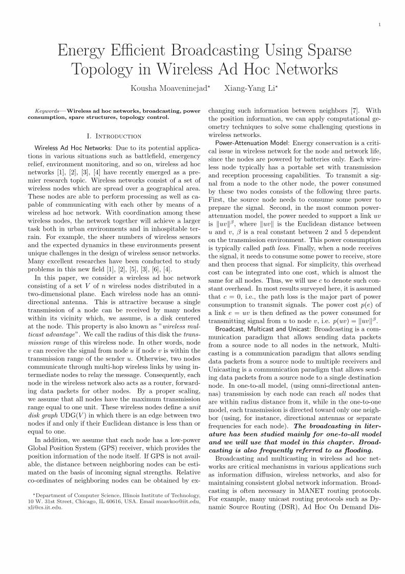
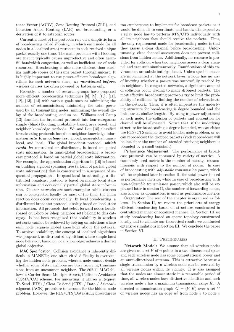
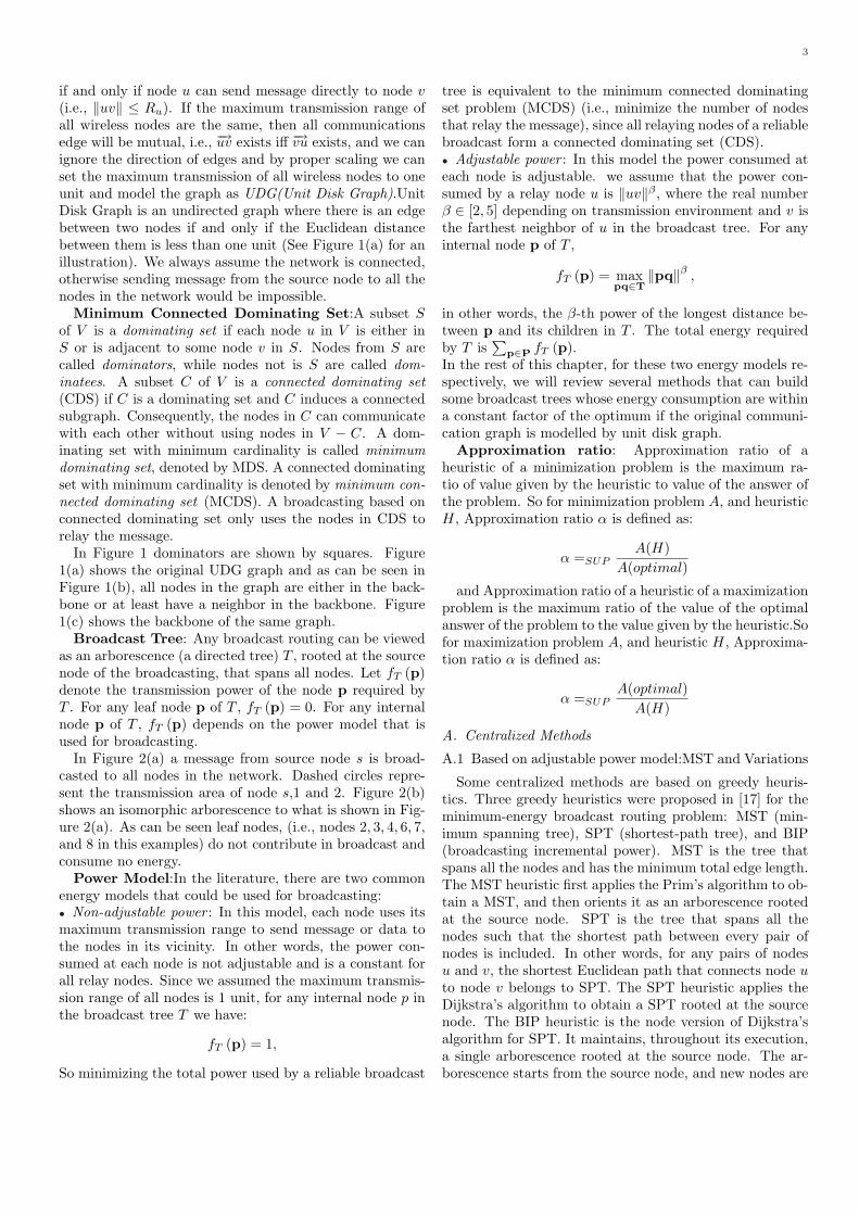
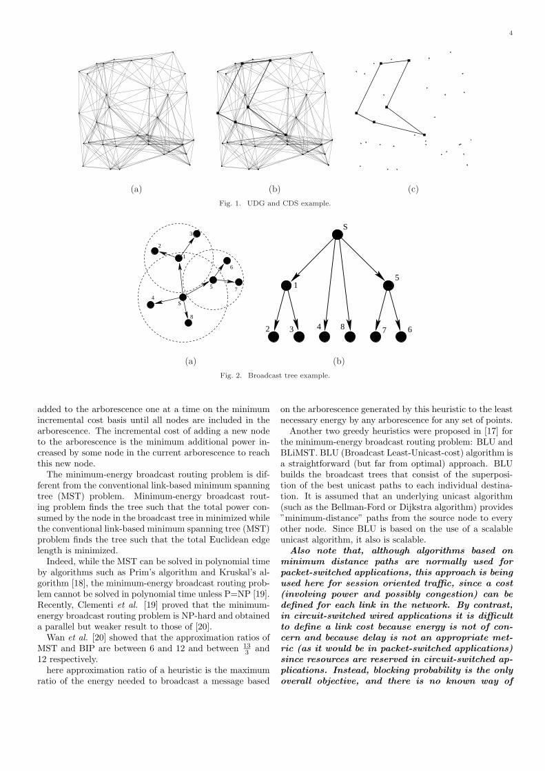
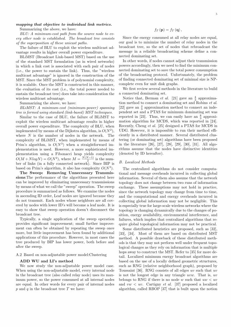
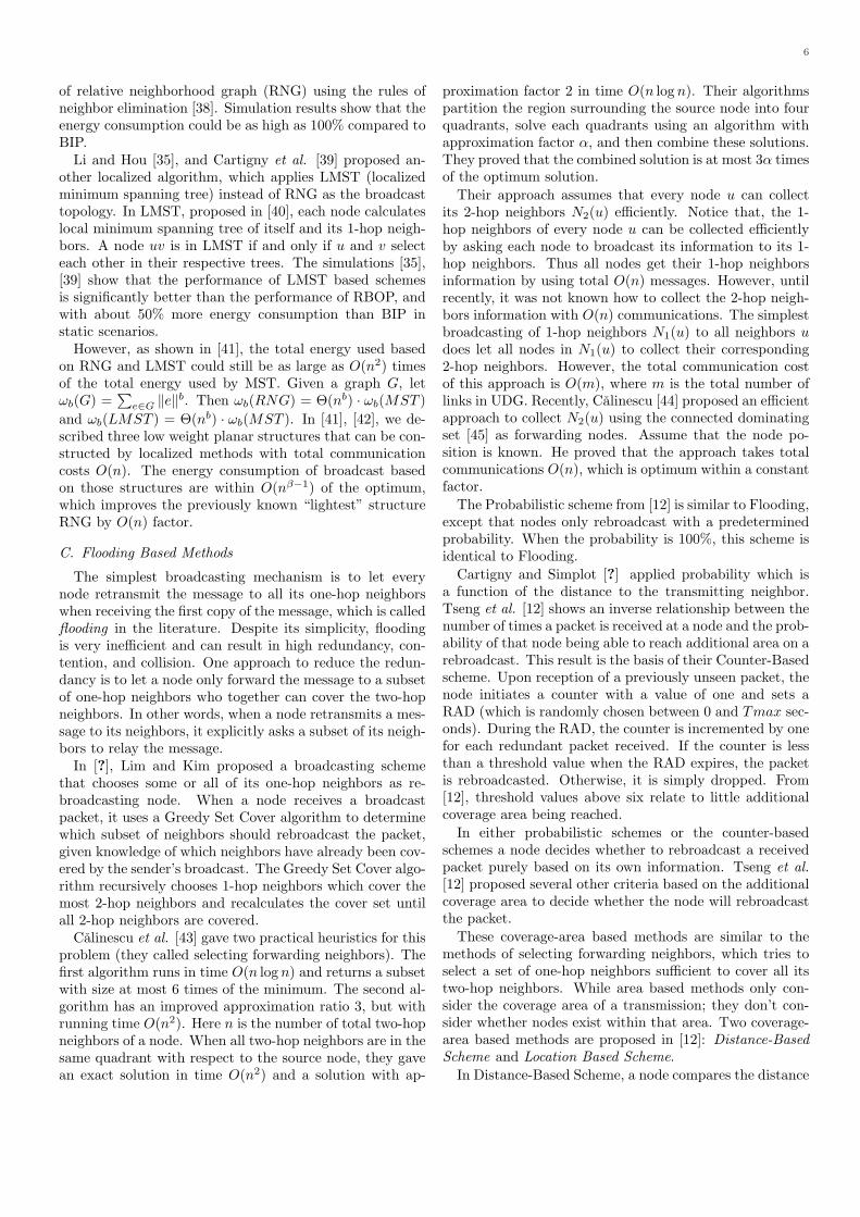
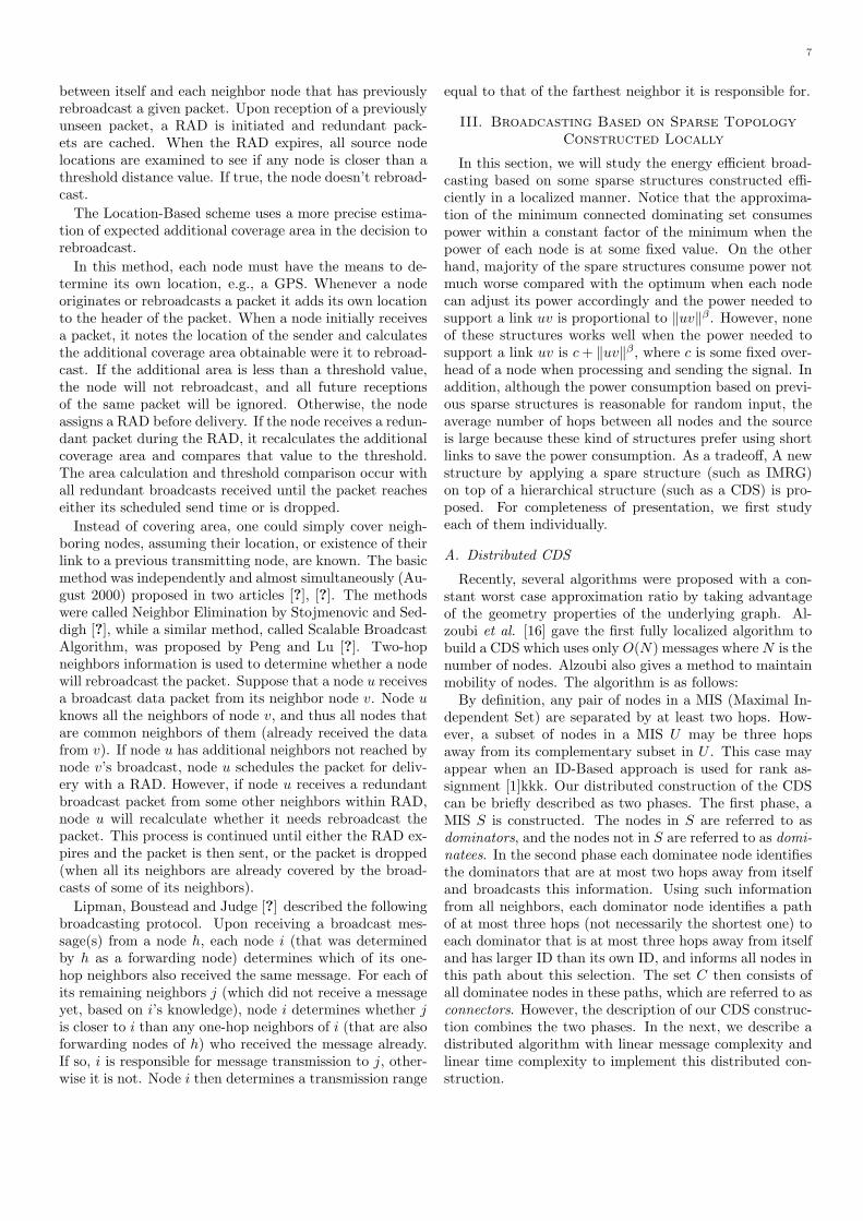
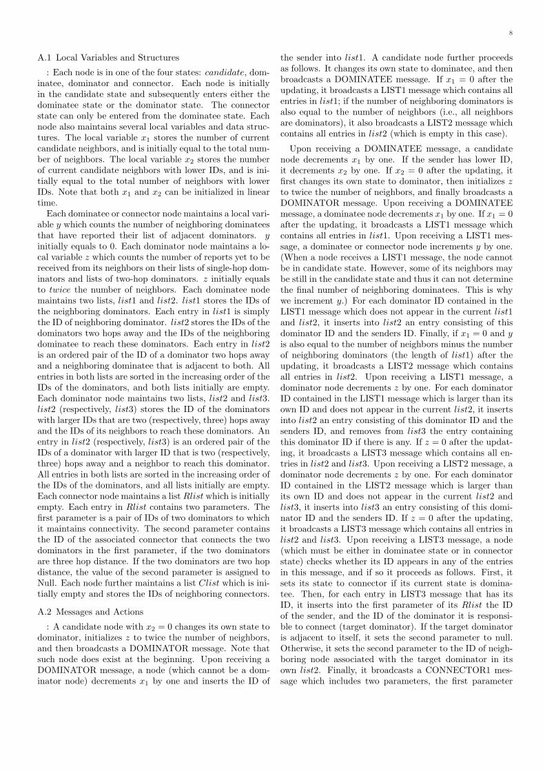
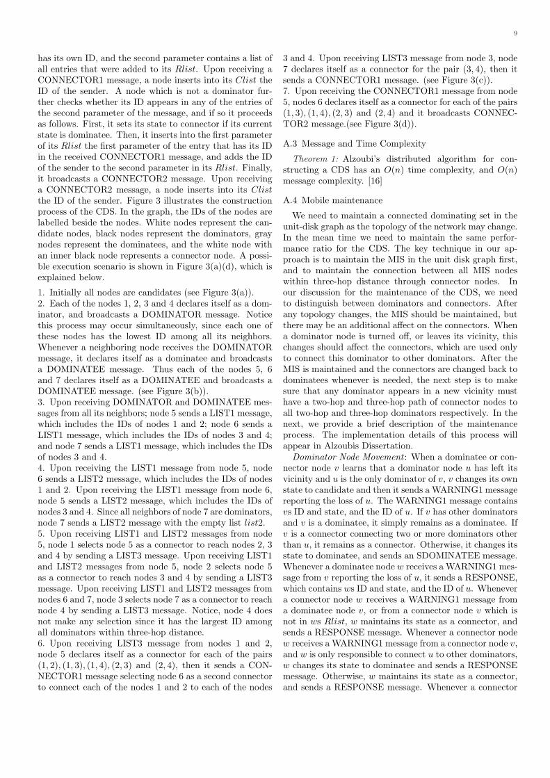
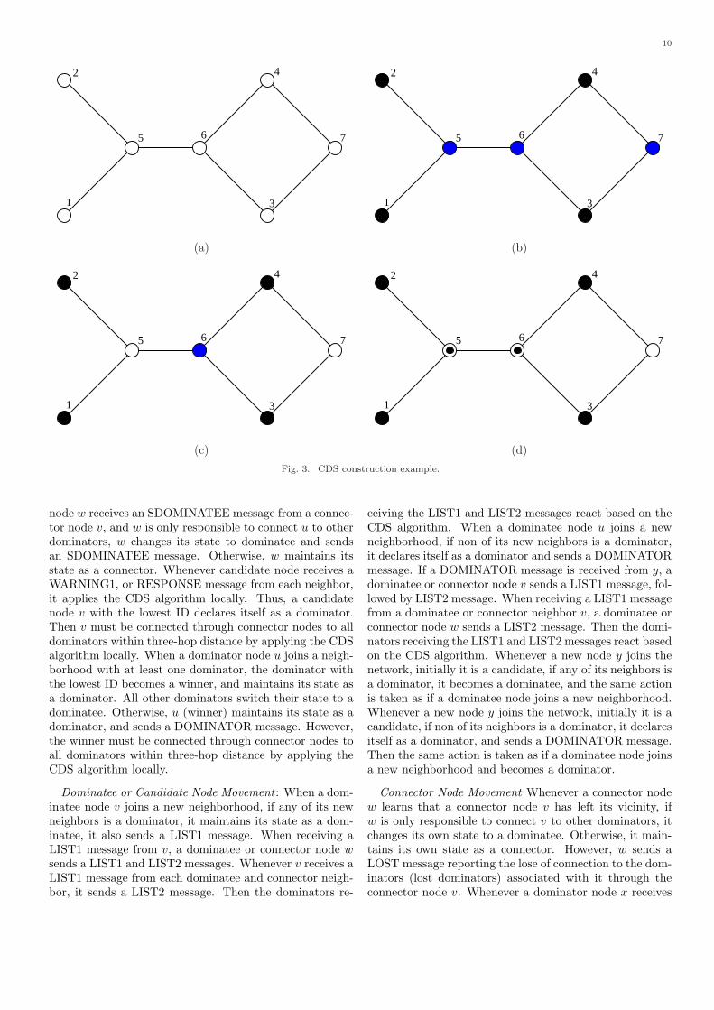
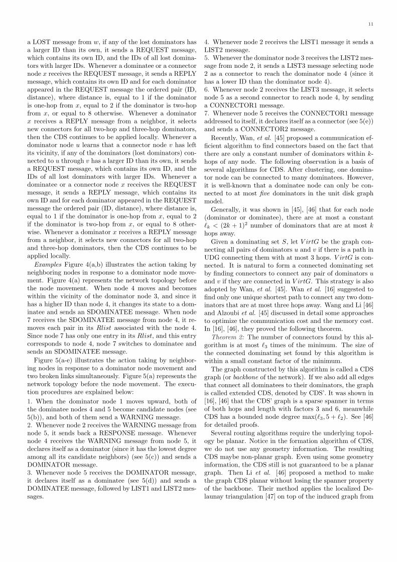
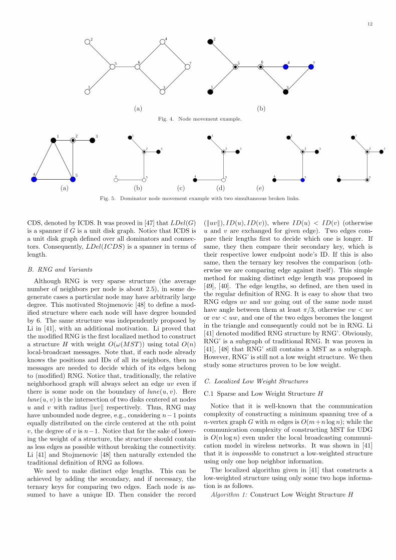
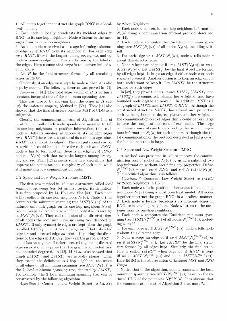
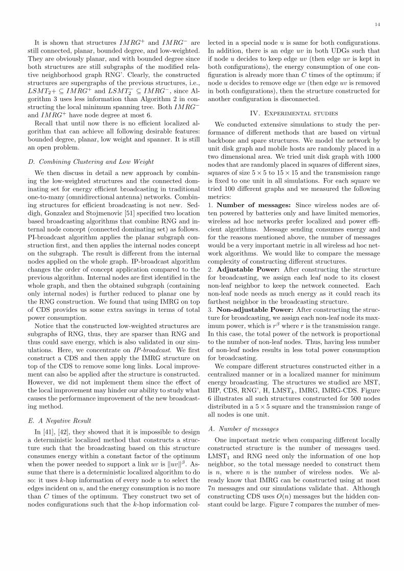
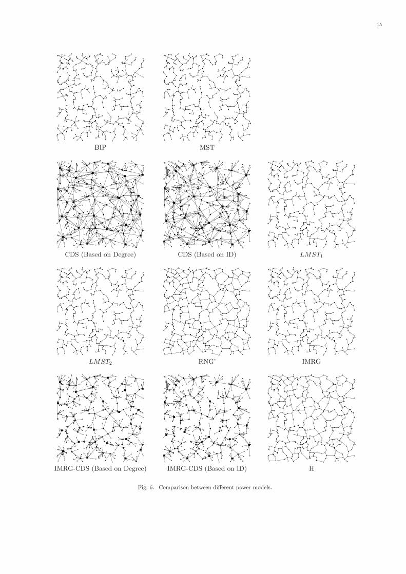
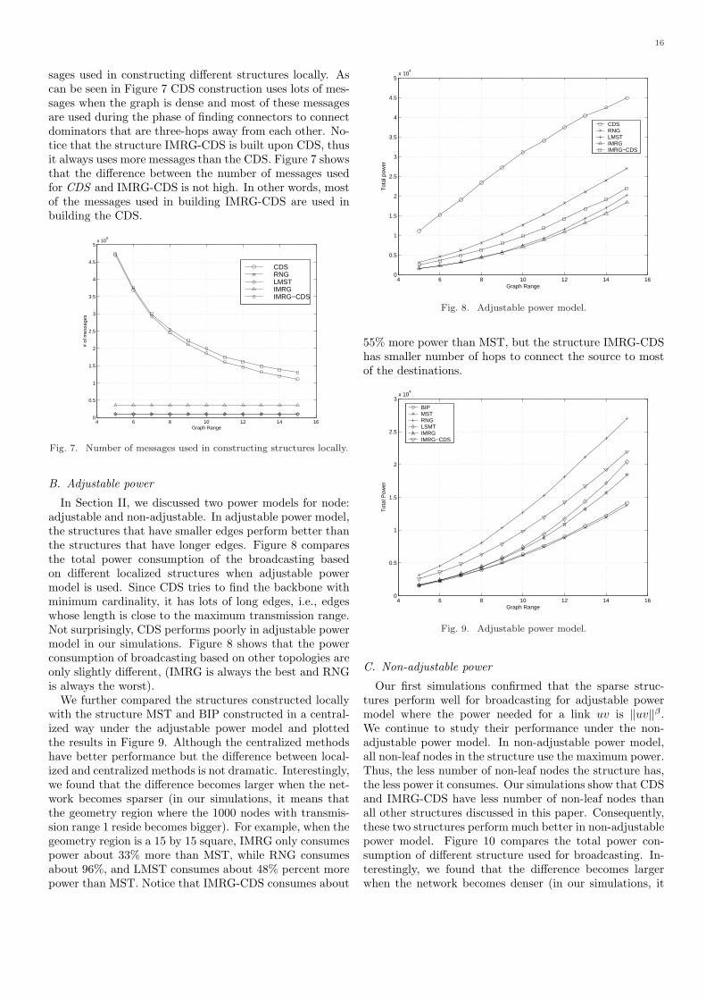
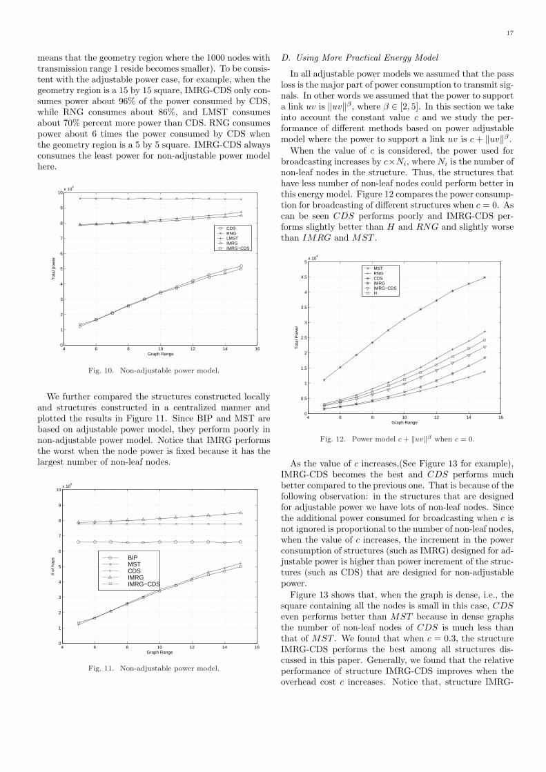
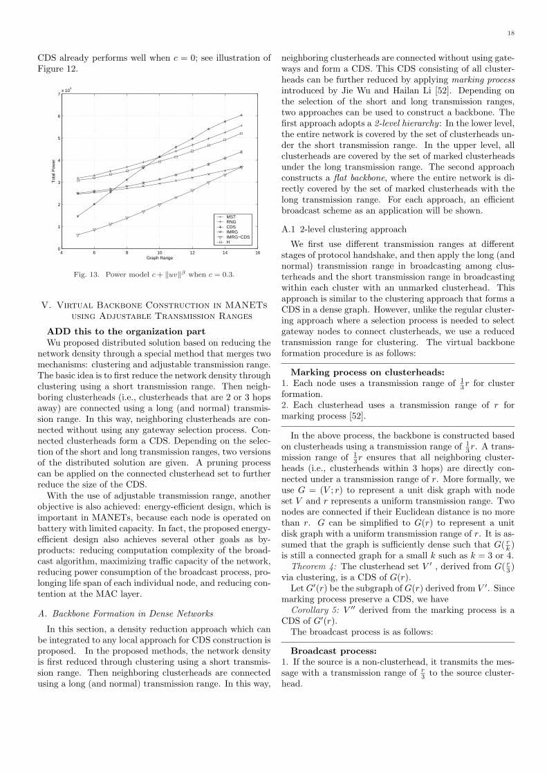
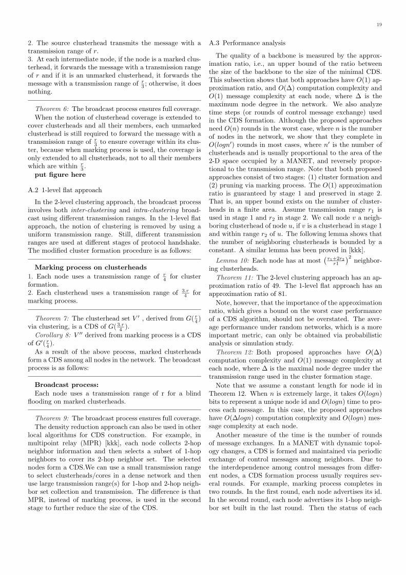
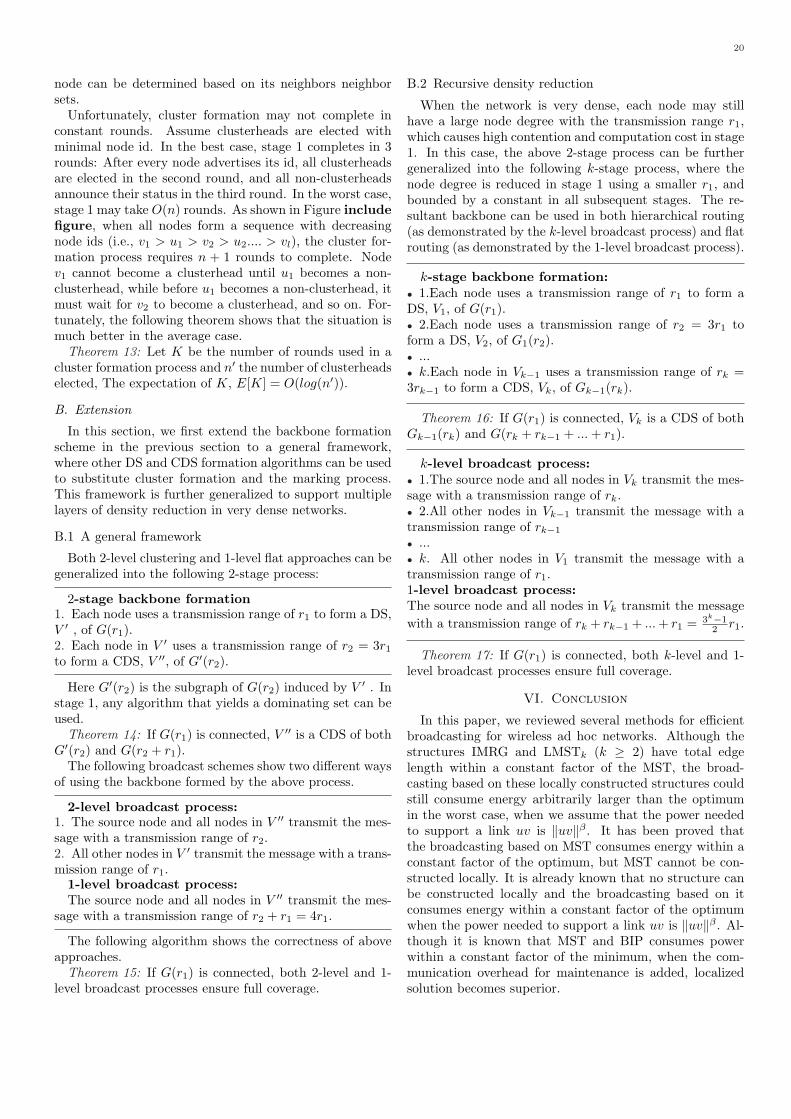
![1 Two Unicast Information Flows over Linear Deterministic ...web.eng.ucsd.edu/~sukamath/two_unicast_linear... · unicast problem, in [1] Wang and Shroff study the solvability of two-unicast](https://static.documents.pub/doc/80x56/6107c99ad649e33b30210889/1-two-unicast-information-flows-over-linear-deterministic-webengucsdedusukamathtwounicastlinear.jpg)


