MEASURING INFLATION: AN ATTEMPT TO OPERATIONALIZE CARL MENGER’S CONCEPT OF THE INNER VALUE OF MONEY M.M.G. Fase and C.K. Folkertsma ABSTRACT This paper attempts to operationalize Carl Menger’s concept of the ‘innerer Tauschwert des Geldes’, i.e. the inner value of money. Since the change in the inner value of money is the component of price movements which is due to monetary influences, the operationalization provides an alternative measure of inflation. We consider several approaches for gauging the change in the inner value of money. Of these, we use Quah and Vahey’s structural VAR model to identify the price movements in the Netherlands and the EU due to monetary shocks. Key words: core inflation, monetary policy, European Monetary Union JEL codes: E31
Transcript
MEASURING INFLATION: AN ATTEMPT TO OPERATIONALIZE CARL MENGER’S
CONCEPT OF THE INNER VALUE OF MONEY
M.M.G. Fase and C.K. Folkertsma
ABSTRACT
This paper attempts to operationalize Carl Menger’s concept of the ‘innerer Tauschwert des Geldes’,i.e. the inner value of money. Since the change in the inner value of money is the component of pricemovements which is due to monetary influences, the operationalization provides an alternativemeasure of inflation. We consider several approaches for gauging the change in the inner value ofmoney. Of these, we use Quah and Vahey’s structural VAR model to identify the price movements inthe Netherlands and the EU due to monetary shocks.
The main objective of this paper is to identify the component of observable price changes, which isdue to monetary as opposed to real shocks. It attempts to operationalize Carl Menger’s old concept ofthe inner value of money as the true measure for inflation. This operationalization is applied to theNetherlands and the European Union, yielding a measure of price changes, which reflects more closelythe theoretical notion of inflation as a monetary phenomenon.
According to the definition adopted here, inflation is any increase in prices induced by monetaryfactors. Contrary to Friedman’s well-known definition of inflation as ‘a steady and sustained rise inprices’ (Friedman (1963) p. 1), a non-recurring price change is considered as (short-term) inflation aslong as it is due to monetary influences. Clearly, without stating that the price changes are induced bymonetary factors, inflation would not be ‘always and everywhere a monetary phenomenon’ (Friedman(1963), p. 17), since short periods of rising prices may, after all, be due to real factors alone. Theadoption of the broader inflation concept seems justified since in economic theory the importantdistinction is not between the effects of a temporary and a sustained price increase but betweenanticipated and unanticipated changes. Furthermore, from the perspective of monetary policy, it isinteresting to measure any movement in prices brought about by monetary shocks, irrespective ofwhether the movements are temporary or sustained.
This paper is organised as follows. Section 2 argues why the change in the consumer price index (CPI)and comparable indices are inappropriate for measuring inflation. Section 3 goes into Carl Menger’sdistinction between ‘innerer’ and ‘äußerer Tauschwert des Geldes’ which is our main inspiration forthis research (Fase (1986, pp. 9-10)). Section 4 proposes a decomposition of price changes. Fourpossible inflation gauges are examined, the aim being to establish which components of price changesthey identify. Section 5 discusses a method to identify the change in the inner value of money insofaras price rises are caused by monetary shocks. Section 6 applies this method to Dutch and Europeandata. Conclusions are drawn in the final section.
2 CHANGES IN PRICE INDICES AS INFLATION GAUGE
The change in the CPI published monthly is seen by the public and by politicians as the measure ofinflation on an annual basis. The change in this index gauges the increase in expenditure on a packageof goods and services consumed by the representative household. Roughly, the rise in the CPI reflectsthe loss of purchasing power of money as the representative household experiences it. Application ofthis index is justifiable if the aim is to determine changes in the spending potential of households,which are caused by price movements ensuing from changes in monetary policy, or from changes infiscal policy and other real causes. However, this gauge is inappropriate for measuring inflation asdefined by Friedman or price level changes brought about by monetary shocks as the CPI reflectsevery change in consumer prices.
Several attempts have been made to restructure the CPI into a better measure of inflation. For instance,in addition to the ordinary CPI, a price index is published in the Netherlands, which has been adjustedfor changes in indirect taxation and subsidies, and various statistical methods have been developed toidentify the trend component in the change in prices. But even when an adjustment is made for thedirect influence of changed taxes and subsidies on expenditure, the index still reacts to price changeswhich have been generated by second-order effects of tax and subsidy adjustments and other realinfluences. Furthermore, weighting the price index means that some prices will determine the generalprice level thus measured to a greater extent than others. For an assessment of changes in purchasingpower, the weighting scheme has a theoretical foundation but there is no clear rationale for gauginginflation by means of weighting. Finally, the basket of goods consumed by households is but a sub-set
- 2 -
of the goods marketed within the economy. Notably the prices of the various factors of production areleft out of account.
Its partial nature, the weighting aspect and the impossibility to distinguish between real and monetarycauses of price changes make the CPI an unsuitable instrument for gauging inflation. For similarreasons, other frequently used price indices such as the producer price index or the implicit deflator ofgross domestic product do not constitute better tools for measuring inflation either.
3 MENGER’S CONCEPT OF ‘INNERER TAUSCHWERT’
At the end of the nineteenth century, Carl Menger (Menger (1923)) introduced the dual concept of the‘innerer’ (i.e. inner) and the ‘äußerer Tauschwert’ (i.e. outer value) of a commodity, and of money inparticular. By the outer value of a commodity, he meant the price of that commodity or the amount ofmoney, which is to be exchanged for the commodity in equilibrium. Analogously, the outer value ofmoney is its purchasing power, viz. the commodity bundle that can be exchanged for one unit ofaccount. In Menger's terminology the CPI thus measures the change in the outer value of money.While Menger stressed that the ratio at which two goods are exchanged in equilibrium is ultimatelydetermined by the (marginal) subjective valuation of the goods involved, he avers that a change in therelationship may be caused by changes affecting only one of the goods. He calls these changesmovements in the inner value of a good. Analogously, changes in the inner value of money are thoseprice changes, which are due to purely monetary factors.
According to Menger, a decrease in the inner value of money must lead to a proportional increase inall goods prices. After all, if the changes relate solely to money, the relative goods prices will, in hisview, remain unchanged. However, he does acknowledge that a proportional rise in all prices need notnecessarily constitute a fall in the inner value of money, because this may also be caused by realfactors affecting the production of all commodities simultaneously. That is why Menger is scepticalabout the possibility of measuring changes in the inner value of money. He mentions measurementbased on the distribution of price changes as a possible way of operationalization. If all prices rise bythe same percentage, the hypothesis that the inner value of money has fallen is more likely than thehypothesis that the inner value of all goods has gone up to the same extent. The likelihood of thisconclusion rests on the fact that the first explanation relates to the changes in the value of fewerobjects of exchange. If not all goods prices go up by the same percentage, then the change in the innervalue of money could, on the basis of the same argument, be estimated with the aid of the mode of thefrequency distribution of the price changes. However, Menger indicates himself that the methodbecomes less convincing as the spread of the price changes increases.
Menger’s concept of the inner value of money is closely related to the definition of inflation used inthis paper. Inflation is the change in the inner value of money. Thus Menger’s classical concept of theinner value of money turns out to have a very modern interpretation. This was already observed byHayek (1934, p. XXXI) who noted that ‘the actual terms employed are somewhat misleading’ but ‘theunderlying concept of the problem is extra-ordinarily modern’. In the light of the relevance ofMenger’s concept it is interesting to search for a more convincing operationalization. The maincharacteristic of Menger’s concept should, however, remain intact. This characteristic is that a changein the inner value of money should ultimately lead to a proportional rise in all commodity prices. Assuggested by Menger, a suitable starting point for operationalization is the frequency distribution ofprice changes. The following section deals with this approach and discusses possible gauges for thechange in the inner value of money.
- 3 -
4 INNER VALUE OF MONEY: A FRAMEWORK FOR THE DECOMPOSITION OF PRICECHANGES
The observed change in the price of a good may be caused by various factors. The change in relativeand absolute prices may be due to monetary or real causes or an error of measurement may haveoccurred. If ktP is the price of good k at time t and
)1(lnln −−= tkktkt PPπis the increase in the price of good k, then the observed price change may be broken down into
ktktktMtkt εβααπ +++= .,...,1 Kk = (1)
ktMt αα + is the price rise at time t of good k, which is underlain by monetary factors, such as an
expansion of the money supply. Although an expansion of the money supply should, at least in thelong run, lead to a proportional rise in all prices, the transmission of monetary shocks will, at least
temporarily, disturb relative prices. Mtα is the change in the inner value of money, i.e. the
proportional rise in all goods prices as a result of a monetary shock following the completion of alladjustment processes. ktα reflects the temporary deviation of the relative prices from the new long-run
equilibrium during the transmission of a monetary shock 1. ktε is the error of measurement which may
arise in the observation of prices. ktβ is the price change in period t which is caused by real factors.
Real shocks may effect a change in supply and demand in all markets. This disturbance of the generalequilibrium of the economy will, if the equilibrium is stable, lead to new relative prices.
The component of the price changes that must be identified is the change in the inner value of moneyMtα . The decomposition of price changes according to (1) may help to examine to what extent the
measuring results obtained with the aid of various inflation gauges will approximate the change in theinner value of money. The first gauge to be considered here is the change in the CPI as the gauge most
commonly used in practice. For the change in the CPI, say Ctπ , which is defined as the weighted sum
of individual price changes by
∑=k
ktktCt w ππ , (2)
with 0)1(0
)1(0 >=∑ −
−
itii
tkkkt Px
Pxw and ∑ =
kktw 1, one has, in view of the decomposition (1) that
∑ ∑ ∑+++=k k k
ktktktktktktMt
Ct www εβααπ . (3)
We see that the change in the CPI does not simply measure the change in the inner value of moneyMtα . We note that, generally speaking, neither the weighted sum of the relative price effects of
transmission ∑k
ktktw α , nor the sum of the budget-share weighted price changes caused by real
factors ∑k
ktktw β equal 0 2. Finally, it cannot be ruled out that measurement errors — the term
∑k
ktktw ε — affect Ctπ .
1 In his discussion of the inner value of money, Menger abstracted from the problem that monetary shocks might lead to atemporary disturbance in relative prices.
2 0=∑k
ktktw β holds only if the demand and supply functions of the economy fulfill highly exceptional conditions.
- 4 -
However, other inflation gauges based on, for instance, the frequency distribution of price changes,may be considered. As the change in the inner value of money is a component of the general price rise,the average, the median or, as Menger proposed, the modal price changes form alternative ways ofmeasuring inflation.
The average price change Atπ would only identify the change in the inner value of money if it may be
assumed that the average price rise caused by real factors and transmission equals nil. After all
∑=k
ktAt K
ππ 1, and, on the basis of decomposition (1)
∑ ∑ ∑+++=k k k
ktktktMt
At KKK
εβααπ 111
or, if the calculation of the average price changes is based on a large number of goods
∑ ∑++≈k k
ktktMt
At KK
βααπ 11. (4)
The latter equation follows under mild conditions from the law of large numbers 3. There are,however, no arguments in economic theory to justify the hypothesis that the relative price changes
caused by real or monetary factors average nil. In fact, it is extremely unlikely that ∑k
ktKβ1
equals
zero after an increase in VAT by 1%. Therefore, the average price change as such is not a suitablestatistic for the change in the inner value of money.The median and the modal price change, too, lead to a breakdown of the changes in the inner value ofmoney and price changes caused by real factors only on the basis of certain ad hoc assumptions. For
the median price change Mtπ , and the modal price change X
tπ ,
tMt
Mt z+= απ (5)
and
tMt
Xt s+= απ (6)
respectively, with z the median and s the mode of the joint distribution of ktα , ktβ and the
measurement errors ktε . Like the change in the CPI and the average price change, the median and the
modal price change are also on the whole unable to identify the change in the inner value of money. Itis clear from this discussion that the changes in the inner value of money cannot be gleaned with theaid of purely descriptive statistics. None of the gauges is capable of distinguishing between generalprice level increases caused by monetary factors and those resulting from real shocks. In addition, allgauges, except the average price change, are sensitive to errors of measurement. Therefore, we followanother route to identify the changes in the inner value of money.
5 THE MODEL OF QUAH AND VAHEY AND THE INNER VALUE OF MONEY
5.1 The model
Quah and Vahey (1995) recently proposed a model for solving the problem of measuring monetaryinflation. This is a structural VAR model. The approach of Quah and Vahey is underlain by the notionthat in the long run inflation, being a monetary phenomenon, is output-neutral, with the proviso thatunexpected inflationary shocks in the short and medium term may influence real income. Measuring
3 Where the change in the CPI is concerned, the law of large numbers applies only under highly implausible assumptions
with regard to the budget shares ktw .
- 5 -
inflation by means of the CPI or other price indices can, however, be misleading as has been shown inthe previous section, since price changes brought about by real factors are not eliminated. Therefore,Quah and Vahey suggest decomposing measured inflation into so-termed core inflation and a residual.Core inflation is defined as the component of measured inflation, which is output-neutral in the longrun.
Quah and Vahey assume that the first differences of (the logarithm of) output and measured inflationare stationary stochastic processes. Furthermore, they assume that the change in measured inflation,
π∆ , and the growth rate of output, y∆ , can be explained by contemporaneous and lagged effects of
two types of shocks 1ε and 2ε . Therefore,
...32
313
22
212
12
111
2
10 +
+
+
+
=
∆∆
−
−
−
−
−
−
t
t
t
t
t
t
t
t
t
t AAAAy ε
εεε
εε
εεπ
(7)
The shocks itε of this structural VAR model are serially and contemporarily uncorrelated with zero
expectation and unit variance 4. Finally, they assume that one of the shocks, the ‘core inflation shock’,
t1ε , does not affect the level of output in the long run. The change in the output-neutral component of
measured inflation, i.e. the change in core inflation, is then defined as ∑∞
=−=∆
0,111,
jjtj
ct A επ , with 11,jA
the element (1,1) of matrix jA .
The parameters of the stochastic process generating inflation and output are, however, unknown andmust be determined empirically. Here an identification problem arises: only the reduced form of thevector autoregressive representation of (7)
+
∆∆
++
∆∆
+
∆∆
=
∆∆
−
−
−
−
−
−
t
t
pt
pt
pt
t
t
t
t
t
yD
yD
yD
y 2
1
2
22
1
11 ...
υυππππ
(8)
can be estimated. The moving average representation of (7), however,
...32
313
22
212
12
111
2
1 +
+
+
+
=
∆∆
−
−
−
−
−
−
t
t
t
t
t
t
t
t
t
t CCCy υ
υυυ
υυ
υυπ
(9)
shows that the shocks e in the structural form (7) are not identified. Indeed, comparing thecoefficients in (7) and (9) shows that tt A ευ 0= and ii AAC =0 , ,...2,1=i with the matrix 0Aunknown.
With the aid of the estimated covariance matrix of the reduced-form disturbances Ω=TttυυE and the
hypothesis that in the long run core inflation is output-neutral, all elements of 0A can be identified.
After all, TTtt AA 00E =υυ so that the covariance matrix yields three restrictions for the four elements
of 0A . The neutrality of core inflation implies that the model parameters must meet a fourth restriction:
after k periods, a core inflation shock leads to a change in the output level of size ∑ =+k
j jkt A0 21,1ε . On
the basis of neutrality, 00 21, =∑∞
=j jA should therefore hold. In other words, the element (2,1) of
matrix 00∑∞
=i i AC must equal zero.
Once the matrix 0A has been determined with the aid of these restrictions, the structural form (7) can
be constructed using the residuals and the estimated parameters from the reduced form (8).
4 The normalization of the variance of the structural shocks does not have any consequences for the estimations of otheroutcomes of the model.
- 6 -
Subsequently, core inflation or the output-neutral component of measured inflation, which is notdirectly observable, may be derived from the parameters and the shocks of the structural form.
5.2 A closer look at the model
Quah and Vahey assume that observed inflation and output are explained by no more than two typesof exogenous shocks. The reasons why core inflation depends on just one type of exogenous shock arethat it is due entirely to monetary influences and that monetary policy is conducted by a singleinstitution, viz. the central bank. The assumption that all other changes in measured inflation andoutput may be explained by a single second type of shock which invariably influences the twoendogenous variables in the same way may be seen as no more than an approximation. The latterassumption can, however, be relaxed if the number of endogenous variables in the model is increasedby the number and nature of possible structural shocks. A desirable extension of the model wouldconsist of the explicit treatment of indirect tax rate changes. It seems unlikely that the effect of achanged VAT rate is identical to that of an oil price change or of a variation in government spending.
In Quah and Vahey’s model, the identification of structural shocks is underlain by the economichypothesis that in the long run inflation does not affect output. There seems to be a consensus amongeconomists about this property of inflation. Inflation is a monetary phenomenon and thus, in theabsence of money illusion, it has no long-run real impact. The bone of contention lies mainly with theshort-run effects of inflation or the speed with which the short-run turns into the long-run Phillipscurve. The influence that inflation may have in the short and the medium run on the level of output is,however, not restricted by the identification method. The model of Quah and Vahey also permits thevalidity of the identification method to be tested. As inflation is a monetary phenomenon, the secondtype of shocks, viz. output shocks, should, in the long run, not affect measured inflation. However,should measured inflation be found to be influenced by output shocks even in the long run, doubtswould arise about the validity of the identification procedure proposed by Quah and Vahey.
Finally, there is an identification problem related to the model of Quah and Vahey. As the model isestimated in first differences of the endogenous variables, it is not core inflation itself that is identified,but the change in core inflation. The level of core inflation itself remains unknown and undetermined.
5.3 The relationship between the inner value of money and core inflation
The main question that arises upon consideration of Quah and Vahey’s model is what relationshipexists between the change in the inner value of money and Quah and Vahey’s concept of coreinflation.
Quah and Vahey’s core inflation is that part of measured inflation which is output-neutral in the longrun. The decompositions of two possible inflation gauges, viz. the change in the CPI of equation (3)and the average price change of equation (4), indicate that in the long run three components do notaffect the level of output, and may therefore be identified as part of core inflation. These componentsare- the change in the inner value of money- the (weighted) average of temporary relative price changes brought about by monetary shocks,
and- measurement errors.Of course, the (weighted) average of the relative price changes generated by monetary shocks isoutput-neutral in the long run because these price effects will disappear if the equilibrium is stable.
Consequently, it may be concluded that the method of Quah and Vahey is, in theory, capable ofdecomposing the influence of real and monetary shocks on inflation, measured by one of these twogauges. However, for both gauges, Quah and Vahey’s core inflation does not correspond wholly to thechange in the inner value of money. Core inflation derived from the CPI or the average price change attime t is the (weighted) average of the price changes at that time, insofar as caused by monetary
- 7 -
factors, but not the change in the inner value of money, i.e. the proportional change in all pricesfollowing a monetary shock after the new long-run equilibrium is reached. Thus, in the absence ofmeasurement errors, the difference between core inflation and the decrease in the inner value ofmoney depends on transitory relative price changes due to monetary shocks.
The use of the unweighted average price change as the inflation series which is to be decomposed byQuah and Vahey’s model probably yields the least distorted estimation of the change in the inner valueof money because, on the one hand, weighting the CPI in order to measure inflation is theoreticallyunfounded and, on the other, errors of measurement have a negligible effect on this inflation gauge.Moreover, when calculating the average price, one is in principle not limited to consumer commoditiesonly. For the other two gauges, the median and the modal price change, it is not possible to determine,without the aid of further and highly detailed assumptions, which components would be identified ascore inflation by the Quah and Vahey method.
Although Quah and Vahey’s core inflation does not exactly correspond to the change in the innervalue of money, core inflation derived from the average price change is thus far the best availableoperationalization to measure Menger’s concept. In the next section we use this operationalization tocalculate the change of the inner value of money for the Netherlands and for the European Union.
6 MEASURING THE INNER VALUE OF MONEY
6.1 The Netherlands
Quah and Vahey’s VAR model (8) for the Netherlands is estimated with monthly data from the period1991-1995. For real output the deseasonalized average daily output of the production industriesexcluding construction was chosen. For observed inflation we used the average price change,calculated on the basis of the 200 price series which also underlie the CPI.
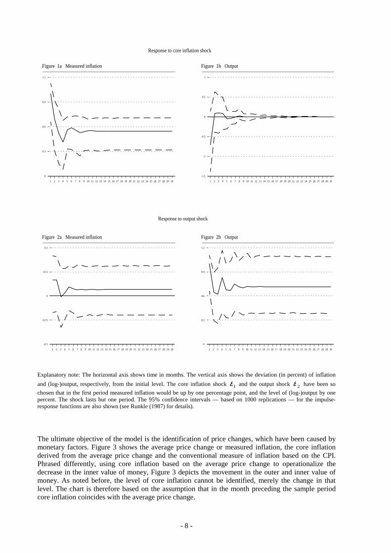
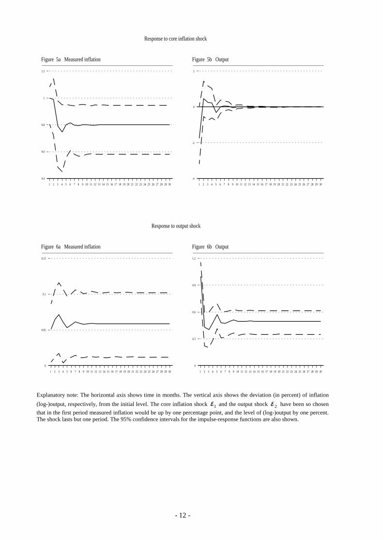
Before estimating Quah and Vahey’s VAR model, we tested if the non-stationarity assumptions areindeed satisfied by the Dutch data. The results of the tests for the non-stationarity of the average pricechange and real output, summarised in Table 1 of Appendix I, indicate that the series are integrated oforder one. Completing the specification of the model, we determined the order of the VAR model.Based on preliminary estimations we included 3 lagged variables in our final model 5. The results ofthe estimation are presented as impulse-response functions shown in Figure 1 and 2, which indicatehow real output and measured inflation respond to the structural shocks. Note that these impulse-responses show the movements in the level of measured inflation and output.
Figure 1 shows that a core inflation shock leads to a permanent increase in inflation, while after lessthan a year output has returned to its initial level. The speed with which the effect of an unanticipatedinflation impulse on real output wears off is not determined by the identification method. Indeed, theidentification implies solely that core inflation has become output-neutral after an infinite number ofperiods. It is noteworthy that an inflation shock decreases output in the first month, while the oppositewas to be expected on the basis of the short-run Phillips curve. The confidence intervals are, however,so large that there is no telling whether this effect is significant.
Figure 2 shows that an output shock leads to a permanent rise in measured inflation, too. This effect is,however, not significant. This confirms the hypothesis that core inflation shocks do indeed reflectmonetary influences. Finally, Figure 2 shows that an output shock has a permanent impact on realoutput.
5 Details are provided in Appendix I.
- 8 -
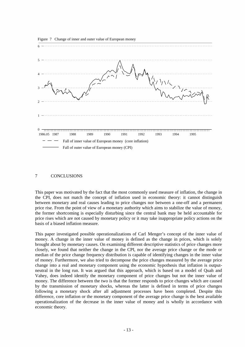
Explanatory note: The horizontal axis shows time in months. The vertical axis shows the deviation (in percent) of inflation
and (log-)output, respectively, from the initial level. The core inflation shock 1ε and the output shock 2ε have been so
chosen that in the first period measured inflation would be up by one percentage point, and the level of (log-)output by onepercent. The shock lasts but one period. The 95% confidence intervals — based on 1000 replications — for the impulse-response functions are also shown (see Runkle (1987) for details).
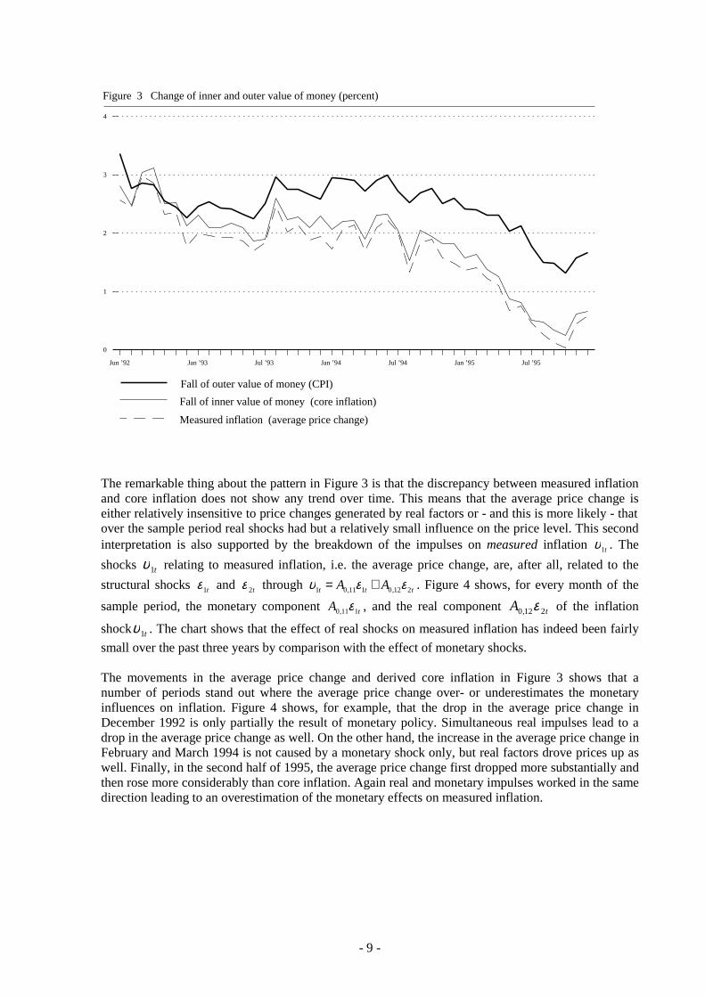
The ultimate objective of the model is the identification of price changes, which have been caused bymonetary factors. Figure 3 shows the average price change or measured inflation, the core inflationderived from the average price change and the conventional measure of inflation based on the CPI.Phrased differently, using core inflation based on the average price change to operationalize thedecrease in the inner value of money, Figure 3 depicts the movement in the outer and inner value ofmoney. As noted before, the level of core inflation cannot be identified, merely the change in thatlevel. The chart is therefore based on the assumption that in the month preceding the sample periodcore inflation coincides with the average price change.
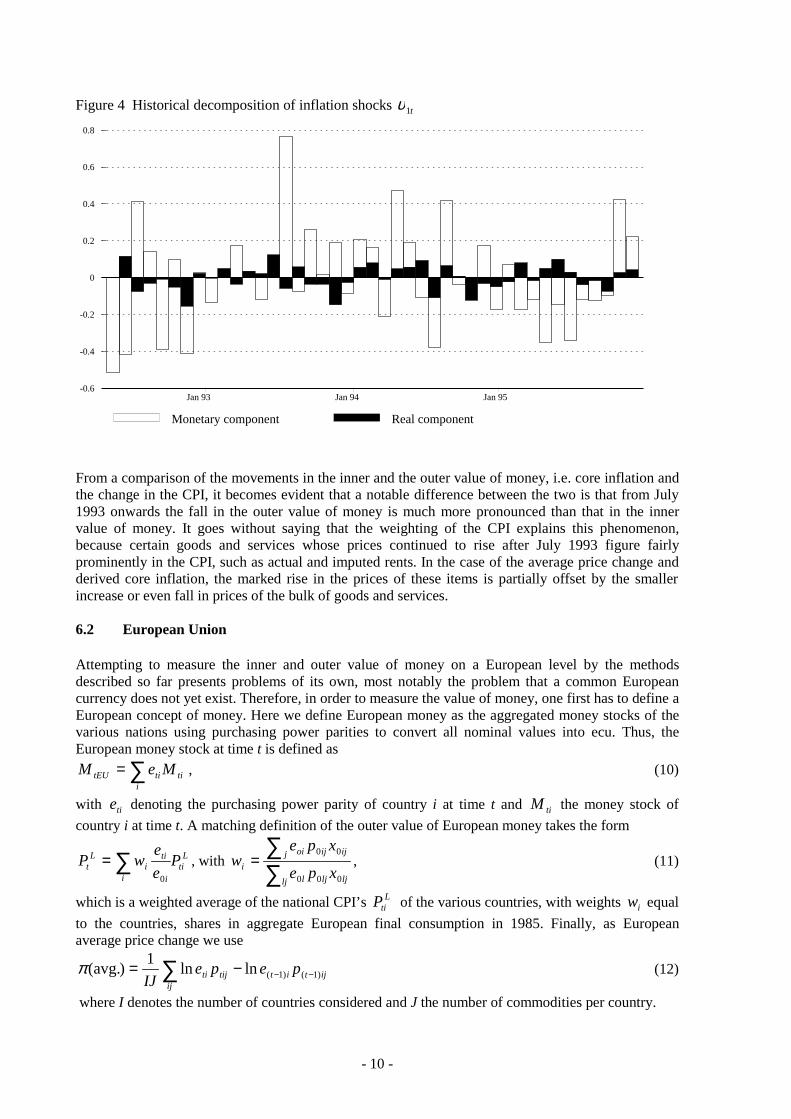
The remarkable thing about the pattern in Figure 3 is that the discrepancy between measured inflationand core inflation does not show any trend over time. This means that the average price change iseither relatively insensitive to price changes generated by real factors or - and this is more likely - thatover the sample period real shocks had but a relatively small influence on the price level. This secondinterpretation is also supported by the breakdown of the impulses on measured inflation t1υ . The
shocks t1υ relating to measured inflation, i.e. the average price change, are, after all, related to the
structural shocks t1ε and t2ε through ttt AA 212,0111,01 εευ += . Figure 4 shows, for every month of the
sample period, the monetary component tA 111,0 ε , and the real component tA 212,0 ε of the inflation
shock t1υ . The chart shows that the effect of real shocks on measured inflation has indeed been fairly
small over the past three years by comparison with the effect of monetary shocks.
The movements in the average price change and derived core inflation in Figure 3 shows that anumber of periods stand out where the average price change over- or underestimates the monetaryinfluences on inflation. Figure 4 shows, for example, that the drop in the average price change inDecember 1992 is only partially the result of monetary policy. Simultaneous real impulses lead to adrop in the average price change as well. On the other hand, the increase in the average price change inFebruary and March 1994 is not caused by a monetary shock only, but real factors drove prices up aswell. Finally, in the second half of 1995, the average price change first dropped more substantially andthen rose more considerably than core inflation. Again real and monetary impulses worked in the samedirection leading to an overestimation of the monetary effects on measured inflation.
1
Jun ’92 Jan ’93 Jul ’93 Jan ’94 Jul ’94 Jan ’95 Jul ’95
0
1
2
3
4
Figure 3 Change of inner and outer value of money (percent)
Fall of outer value of money (CPI)
Fall of inner value of money (core inflation)
Measured inflation (average price change)
- 10 -
Figure 4 Historical decomposition of inflation shocks t1υ
From a comparison of the movements in the inner and the outer value of money, i.e. core inflation andthe change in the CPI, it becomes evident that a notable difference between the two is that from July1993 onwards the fall in the outer value of money is much more pronounced than that in the innervalue of money. It goes without saying that the weighting of the CPI explains this phenomenon,because certain goods and services whose prices continued to rise after July 1993 figure fairlyprominently in the CPI, such as actual and imputed rents. In the case of the average price change andderived core inflation, the marked rise in the prices of these items is partially offset by the smallerincrease or even fall in prices of the bulk of goods and services.
6.2 European Union
Attempting to measure the inner and outer value of money on a European level by the methodsdescribed so far presents problems of its own, most notably the problem that a common Europeancurrency does not yet exist. Therefore, in order to measure the value of money, one first has to define aEuropean concept of money. Here we define European money as the aggregated money stocks of thevarious nations using purchasing power parities to convert all nominal values into ecu. Thus, theEuropean money stock at time t is defined as
∑=i
tititEU MeM , (10)
with tie denoting the purchasing power parity of country i at time t and tiM the money stock of
country i at time t. A matching definition of the outer value of European money takes the form
Lti
i i
tii
Lt P
e
ewP ∑=
0
, with ∑∑
=lj ljljl
j ijijoi
i xpe
xpew
000
00, (11)
which is a weighted average of the national CPI’s LtiP of the various countries, with weights iw equal
to the countries, shares in aggregate European final consumption in 1985. Finally, as Europeanaverage price change we use
ijtij
ittijti pepeIJ )1()1(lnln1
)avg.( −−∑ −=π (12)
where I denotes the number of countries considered and J the number of commodities per country.
1
Jan 93 Jan 94 Jan 95-0.6
-0.4
-0.2
0
0.2
0.4
0.6
0.8
Monetary component Real component
- 11 -
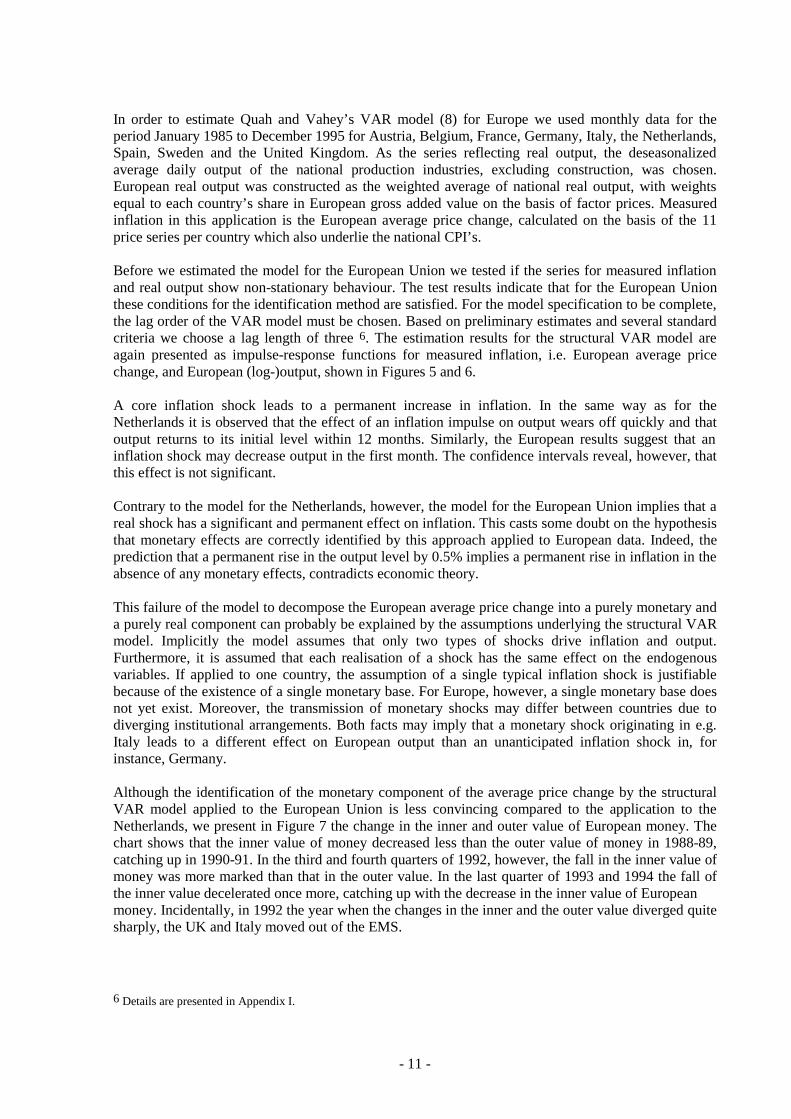
In order to estimate Quah and Vahey’s VAR model (8) for Europe we used monthly data for theperiod January 1985 to December 1995 for Austria, Belgium, France, Germany, Italy, the Netherlands,Spain, Sweden and the United Kingdom. As the series reflecting real output, the deseasonalizedaverage daily output of the national production industries, excluding construction, was chosen.European real output was constructed as the weighted average of national real output, with weightsequal to each country’s share in European gross added value on the basis of factor prices. Measuredinflation in this application is the European average price change, calculated on the basis of the 11price series per country which also underlie the national CPI’s.
Before we estimated the model for the European Union we tested if the series for measured inflationand real output show non-stationary behaviour. The test results indicate that for the European Unionthese conditions for the identification method are satisfied. For the model specification to be complete,the lag order of the VAR model must be chosen. Based on preliminary estimates and several standardcriteria we choose a lag length of three 6. The estimation results for the structural VAR model areagain presented as impulse-response functions for measured inflation, i.e. European average pricechange, and European (log-)output, shown in Figures 5 and 6.
A core inflation shock leads to a permanent increase in inflation. In the same way as for theNetherlands it is observed that the effect of an inflation impulse on output wears off quickly and thatoutput returns to its initial level within 12 months. Similarly, the European results suggest that aninflation shock may decrease output in the first month. The confidence intervals reveal, however, thatthis effect is not significant.
Contrary to the model for the Netherlands, however, the model for the European Union implies that areal shock has a significant and permanent effect on inflation. This casts some doubt on the hypothesisthat monetary effects are correctly identified by this approach applied to European data. Indeed, theprediction that a permanent rise in the output level by 0.5% implies a permanent rise in inflation in theabsence of any monetary effects, contradicts economic theory.
This failure of the model to decompose the European average price change into a purely monetary anda purely real component can probably be explained by the assumptions underlying the structural VARmodel. Implicitly the model assumes that only two types of shocks drive inflation and output.Furthermore, it is assumed that each realisation of a shock has the same effect on the endogenousvariables. If applied to one country, the assumption of a single typical inflation shock is justifiablebecause of the existence of a single monetary base. For Europe, however, a single monetary base doesnot yet exist. Moreover, the transmission of monetary shocks may differ between countries due todiverging institutional arrangements. Both facts may imply that a monetary shock originating in e.g.Italy leads to a different effect on European output than an unanticipated inflation shock in, forinstance, Germany.
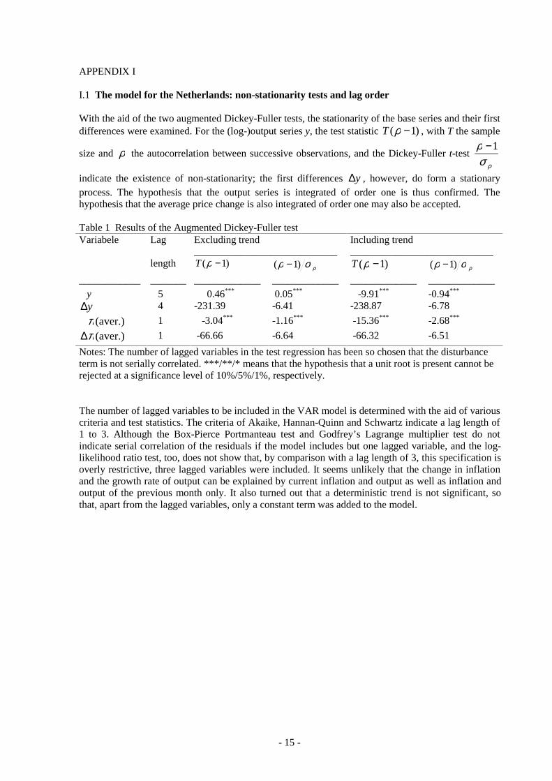
Although the identification of the monetary component of the average price change by the structuralVAR model applied to the European Union is less convincing compared to the application to theNetherlands, we present in Figure 7 the change in the inner and outer value of European money. Thechart shows that the inner value of money decreased less than the outer value of money in 1988-89,catching up in 1990-91. In the third and fourth quarters of 1992, however, the fall in the inner value ofmoney was more marked than that in the outer value. In the last quarter of 1993 and 1994 the fall ofthe inner value decelerated once more, catching up with the decrease in the inner value of Europeanmoney. Incidentally, in 1992 the year when the changes in the inner and the outer value diverged quitesharply, the UK and Italy moved out of the EMS.
6 Details are presented in Appendix I.
- 12 -
Explanatory note: The horizontal axis shows time in months. The vertical axis shows the deviation (in percent) of inflation
(log-)output, respectively, from the initial level. The core inflation shock 1ε and the output shock 2ε have been so chosen
that in the first period measured inflation would be up by one percentage point, and the level of (log-)output by one percent.The shock lasts but one period. The 95% confidence intervals for the impulse-response functions are also shown.
This paper was motivated by the fact that the most commonly used measure of inflation, the change inthe CPI, does not match the concept of inflation used in economic theory: it cannot distinguishbetween monetary and real causes leading to price changes nor between a one-off and a permanentprice rise. From the point of view of a monetary authority which aims to stabilize the value of money,the former shortcoming is especially disturbing since the central bank may be held accountable forprice rises which are not caused by monetary policy or it may take inappropriate policy actions on thebasis of a biased inflation measure.
This paper investigated possible operationalizations of Carl Menger’s concept of the inner value ofmoney. A change in the inner value of money is defined as the change in prices, which is solelybrought about by monetary causes. On examining different descriptive statistics of price changes moreclosely, we found that neither the change in the CPI, nor the average price change or the mode ormedian of the price change frequency distribution is capable of identifying changes in the inner valueof money. Furthermore, we also tried to decompose the price changes measured by the average pricechange into a real and monetary component using the economic hypothesis that inflation is output-neutral in the long run. It was argued that this approach, which is based on a model of Quah andVahey, does indeed identify the monetary component of price changes but not the inner value ofmoney. The difference between the two is that the former responds to price changes which are causedby the transmission of monetary shocks, whereas the latter is defined in terms of price changesfollowing a monetary shock after all adjustment processes have been completed. Despite thisdifference, core inflation or the monetary component of the average price change is the best availableoperationalization of the decrease in the inner value of money and is wholly in accordance witheconomic theory.
Figure 7 Change of inner and outer value of European money
Fall of inner value of European money (core inflation)
Fall of outer value of European money (CPI)
- 14 -
Applying the approach to the Netherlands and the European Union, we found that the change in theinner and that in the outer value of money have diverged considerably and persistently in the periodsexamined. This finding indicates that using the CPI as a gauge for inflation is not only theoreticallyinappropriate but that even in practical applications it yields distorted information on the actualinflationary tendencies. The change in the inner value of money may be seen as an alternative measurethat matches the concept of inflation used in economic theory more closely than the change in the CPI.Moreover, from the point of view of monetary policy, it seems to be the more adequate measure ofinflation in terms of accountability.
- 15 -
APPENDIX I
I.1 The model for the Netherlands: non-stationarity tests and lag order
With the aid of the two augmented Dickey-Fuller tests, the stationarity of the base series and their firstdifferences were examined. For the (log-)output series y, the test statistic )1( −ρT , with T the sample
size and ρ the autocorrelation between successive observations, and the Dickey-Fuller t-test ρσ
ρ 1−
indicate the existence of non-stationarity; the first differences y∆ , however, do form a stationaryprocess. The hypothesis that the output series is integrated of order one is thus confirmed. Thehypothesis that the average price change is also integrated of order one may also be accepted.
Table 1 Results of the Augmented Dickey-Fuller testVariabele Lag Excluding trend Including trend
Notes: The number of lagged variables in the test regression has been so chosen that the disturbanceterm is not serially correlated. ***/**/* means that the hypothesis that a unit root is present cannot berejected at a significance level of 10%/5%/1%, respectively.
The number of lagged variables to be included in the VAR model is determined with the aid of variouscriteria and test statistics. The criteria of Akaike, Hannan-Quinn and Schwartz indicate a lag length of1 to 3. Although the Box-Pierce Portmanteau test and Godfrey’s Lagrange multiplier test do notindicate serial correlation of the residuals if the model includes but one lagged variable, and the log-likelihood ratio test, too, does not show that, by comparison with a lag length of 3, this specification isoverly restrictive, three lagged variables were included. It seems unlikely that the change in inflationand the growth rate of output can be explained by current inflation and output as well as inflation andoutput of the previous month only. It also turned out that a deterministic trend is not significant, sothat, apart from the lagged variables, only a constant term was added to the model.
- 16 -
I.2 The model for the European Union: non-stationarity tests and lag order
The results of the test for the non-stationarity of the European average price change and European realoutput are summarised in Table 2. With the aid of the two augmented Dickey-Fuller tests, thestationarity of the base series and their first differences were examined. For the (log-)output series y,the test statistic )1( −ρT , and the Dickey-Fuller t-test indicate the existence of non-stationarity; the
first differences y∆ , however, do form a stationary process. The hypothesis that the output series isintegrated of order one is thus confirmed. The hypothesis that the average price change is alsointegrated of order one may also be accepted.
Table 2 Results of the Augmented Dickey-Fuller testVariabele Lag Excluding trend Including trend
Notes: The number of lagged variables in the test regression has been so chosen that the disturbanceterm is not serially correlated. ***/**/* means that the hypothesis that a unit root is present cannot berejected at a significance level of 10%/5%/1%, respectively.
As in the model for the Netherlands, the number of lagged variables to be included in the VAR modelis determined with the aid of the criteria of Akaike, Hannan-Quinn and Schwartz. The criterion ofSchwartz points towards a lag length of 1, whereas the other two criteria indicate a lag length of 3. Themodel with 1 lagged variable is, however, not correctly specified since the Box-Pierce Portmanteautest and Godfrey’s Lagrange multiplier test indicate serial correlation of the residuals. The log-likelihood ratio test, too, rejects a lag length of 1 maintaining the model with three lagged variables.
- 17 -
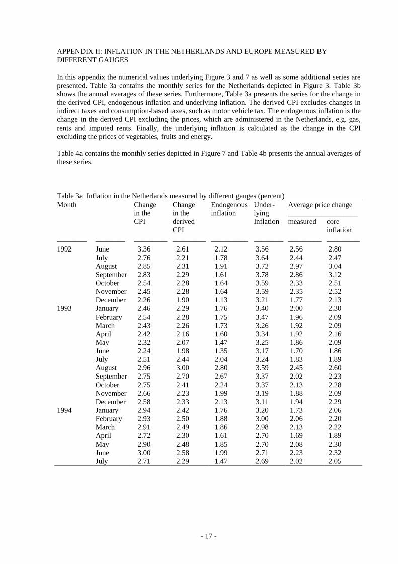
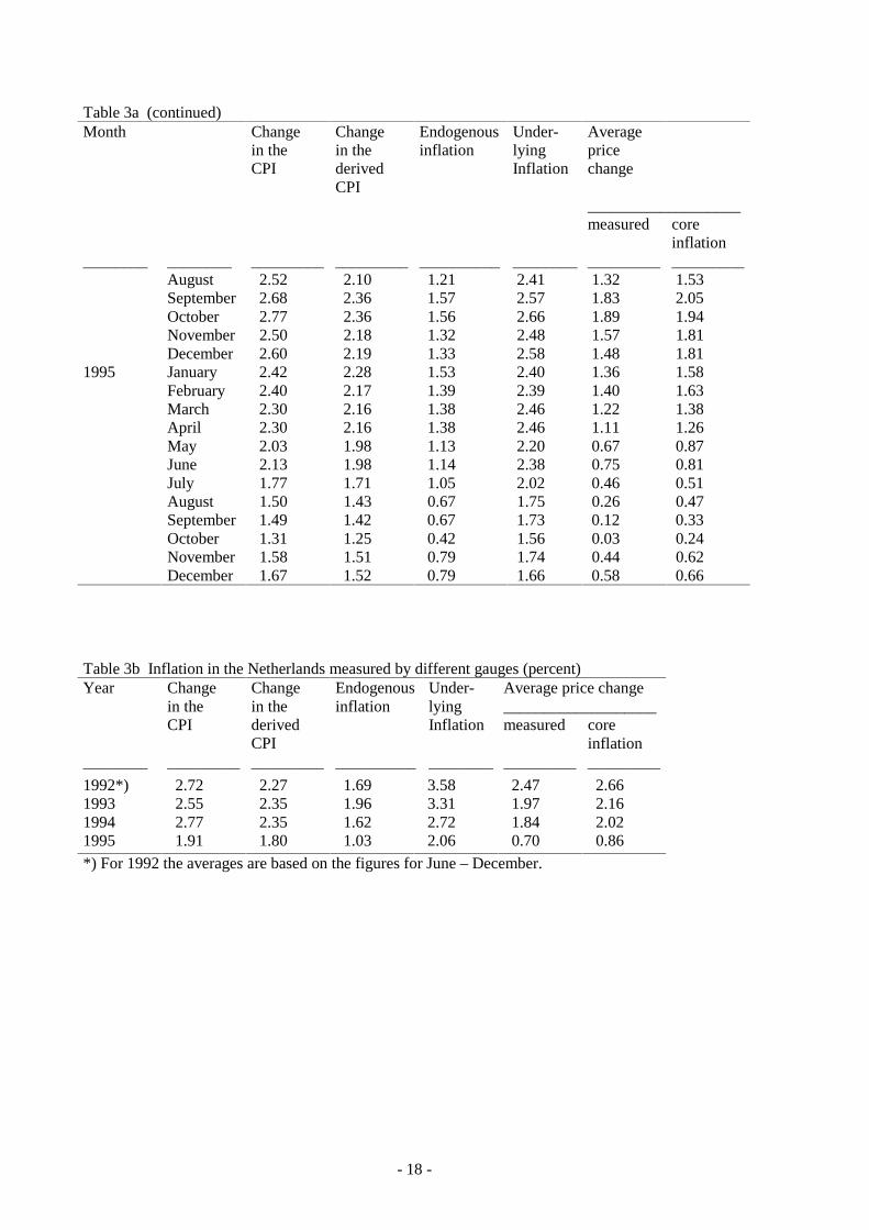
APPENDIX II: INFLATION IN THE NETHERLANDS AND EUROPE MEASURED BYDIFFERENT GAUGES
In this appendix the numerical values underlying Figure 3 and 7 as well as some additional series arepresented. Table 3a contains the monthly series for the Netherlands depicted in Figure 3. Table 3bshows the annual averages of these series. Furthermore, Table 3a presents the series for the change inthe derived CPI, endogenous inflation and underlying inflation. The derived CPI excludes changes inindirect taxes and consumption-based taxes, such as motor vehicle tax. The endogenous inflation is thechange in the derived CPI excluding the prices, which are administered in the Netherlands, e.g. gas,rents and imputed rents. Finally, the underlying inflation is calculated as the change in the CPIexcluding the prices of vegetables, fruits and energy.
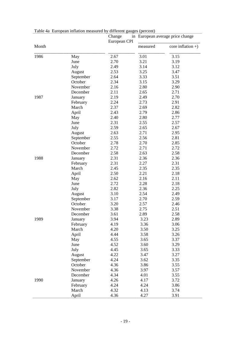
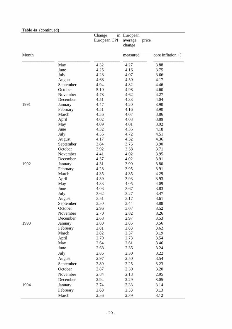
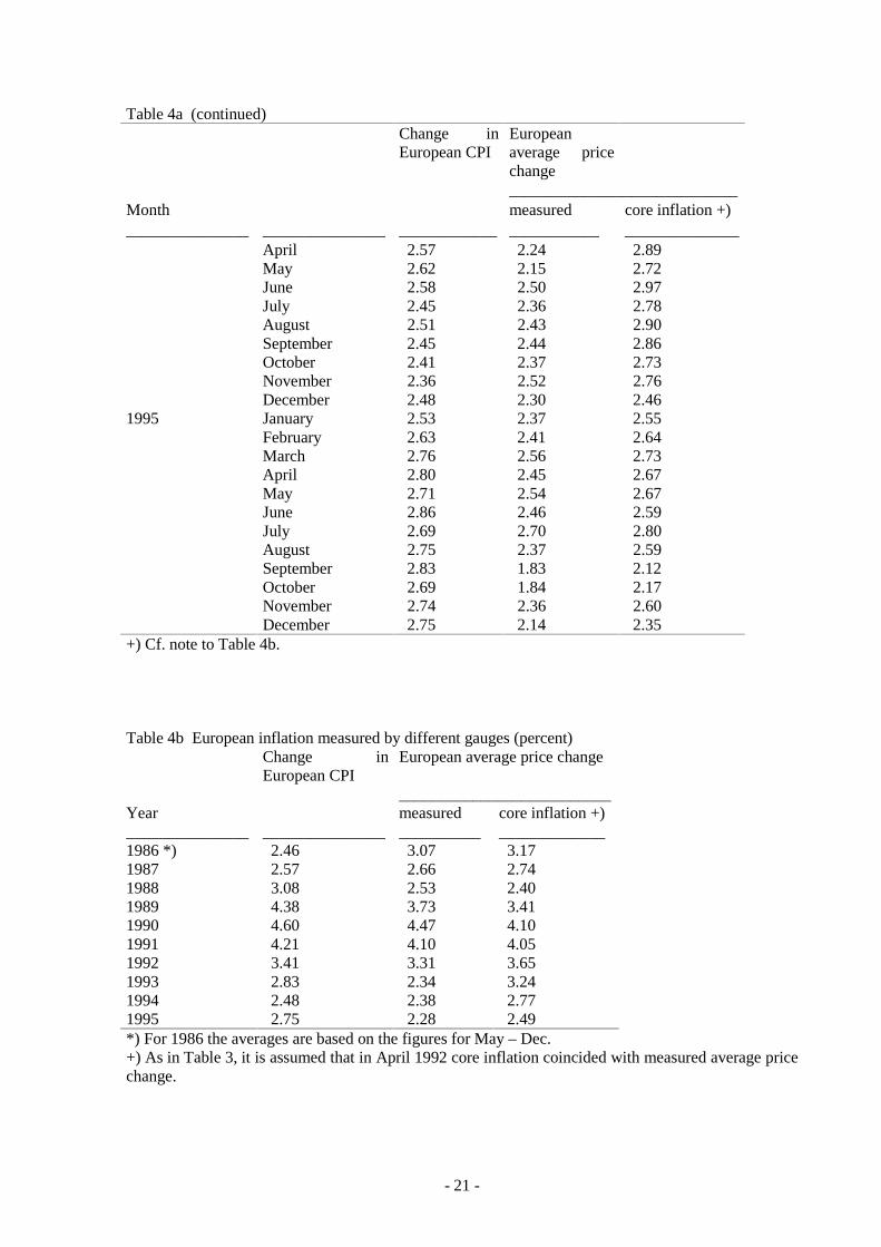
Table 4a contains the monthly series depicted in Figure 7 and Table 4b presents the annual averages ofthese series.
Table 3a Inflation in the Netherlands measured by different gauges (percent)Month Average price change
Table 4b European inflation measured by different gauges (percent)Change inEuropean CPI
European average price change
__________________________Year measured core inflation +)_______________ _______________ __________ _____________1986 *) 2.46 3.07 3.171987 2.57 2.66 2.741988 3.08 2.53 2.401989 4.38 3.73 3.411990 4.60 4.47 4.101991 4.21 4.10 4.051992 3.41 3.31 3.651993 2.83 2.34 3.241994 2.48 2.38 2.771995 2.75 2.28 2.49*) For 1986 the averages are based on the figures for May – Dec.+) As in Table 3, it is assumed that in April 1992 core inflation coincided with measured average pricechange.
- 22 -
REFERENCES
Fase, M.M.G. (1986) ‘Geldtheorie en monetaire normen: enige beschouwingen over aard en inhoudvan de monetaire economie’, Stenfert Kroese: Leiden/Antwerpen.
Friedman, M. (1963) Inflation: Causes and Consequences, Asia Publishing House: New York.
Hayek, F.A. von (1934) ‘Carl Menger’, in The Collected Work of Carl Menger I, MacMillan:London.
Menger, C. (1923, 2nd edition) Grundsätze der Volkswirtschaftslehre, Hölder-Pichler-Tempsky:Wien, Chapter 9.
Quah, D. and S.P. Vahey (1995) ‘Measuring core inflation’, The Economic Journal 105, pp. 1130-1144.
Runkle, D.E. (1987) ‘Vector autoregressions and reality’, Journal of Business and EconomicStatistics 5, pp. 437-442.