1 On Computing Ranges of Polynomials - Some Improvements to the Bernstein Approach P. S. V. Nataraj...

1

On Computing Ranges of On Computing Ranges of Polynomials - Some Polynomials - Some

Improvements to the Improvements to the Bernstein ApproachBernstein Approach

P. S. V. NatarajShashwati Ray

IIT Bombay

Presented at the Second Taylor Model Workshop, Miami, Dec. 2003

Indian Institute of Technology, Bombay 2003

2

SCOPE OF THE PRESENTATIONSCOPE OF THE PRESENTATION Introduction Bernstein forms :

• Definition• Properties• Basis conversion

Range calculations• Important theorems• Subdivision• Subdivision direction selection strategies

New propositions Comparison with Globsol Examples and conclusion Future work

3

INTRODUCTIONINTRODUCTION

Polynomials are encountered in Engineering and Scientific Applications.

Required to find bounds for the range of polynomials over an interval.

Our method based on expansion of multivariate polynomial into Bernstein form.

4

ADVANTAGES OF BERNSTEIN ADVANTAGES OF BERNSTEIN FORMFORM

Avoids function evaluations – may be otherwise costly for polynomials of high degrees.

Nice features about range enclosures with Bernstein form: Information when enclosure is exact.

Sharpness of enclosure can be improved by elevating the Bernstein degree or by subdivision of the domain

5

BERNSTEIN FORMBERNSTEIN FORM

Any polynomial in power form is represented as

Bernstein form of representation is

Bernstein coefficients are given by

RR , , 0

naxaxp i ni

n

ii)(

[0,1] )( )(0

xxBbxp ni

n

i

ni

ni

j

n

j

i

abi

jj

ni ,...,2,1,0

0

,

6

BERNSTEIN FORMBERNSTEIN FORM

Bernstein functions on [0,1] are defined by

On a general interval the Bernstein functions are defined as

Each set of coefficients ai or bin can be computed from the

other (i.e., power form to Bernstein form).

nix)(xi

n(x)B inin

i ,...,2,1,01

,

],[ xxx

x,xxxx

xxxx

i

nxB n

inini

7

BASIS CONVERSIONBASIS CONVERSION On unit interval a polynomial’s equivalent power and

Bernstein forms

Using matrix multiplication p(x) = XA = BXB – X is the variable (row) matrix.– A is the coefficient (column) matrix– BX is the Bernstein basis (row) matrix – B is the Bernstein coefficient (column) matrix

After certain computations, BXB = XUXB– UX is a lower triangular matrix

)()(00

xBbxaxp ni

n

i

ni

n

i

ii

8

BASIS CONVERSIONBASIS CONVERSION

BX = XWXVXUX

– WX is an upper triangular matrix

– VX is a diagonal matrix

XA = BXB

XA = XWXVXUX B

B=(UX)-1 (VX)-1 (WX)-1A

9

BASIS CONVERSIONBASIS CONVERSION

For a bivariate case

X1 and X2 are variable matrices

By analogy with univariate case

TAXXxxp 2121 ),( TXX BBBxxp

21),( 21

1111 1 XXXX UVWXB

2222 2 XXXX UVWXB

10

RANGE CALCULATIONRANGE CALCULATION IMPORTANT THEOREMSIMPORTANT THEOREMS

Theorem 1 : The minimum and maximum Bernstein coefficients give an enclosure of the range of polynomial on the given interval.

Theorem 2 : Vertex condition : If the minimum and maximum Bernstein coefficients of polynomial in Bernstein form occur at the vertices of the Bernstein coefficient array, then the enclosure is the exact range.

Theorem 3 : Bernstein approximations converge to the range and the convergence is at least linear in the order of approximations.

11

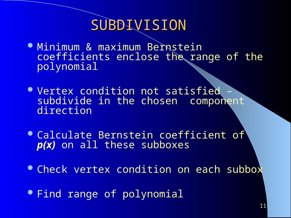
SUBDIVISIONSUBDIVISION Minimum & maximum Bernstein coefficients

enclose the range of the polynomial

Vertex condition not satisfied – subdivide in the chosen component direction

Calculate Bernstein coefficient of p(x) on all these subboxes

Check vertex condition on each subbox

Find range of polynomial

12

SWEEP PROCEDURESWEEP PROCEDURE

13

SUBDIVISION DIRECTION SUBDIVISION DIRECTION SELECTION STRATEGIESSELECTION STRATEGIES

EXISTING RULESEXISTING RULES Rule A

• Direction chosen is cyclic

Rule B (derivative based)• Find an upper bound for the absolute value of the

partial derivative (from its Bernstein form) in the rth direction

• Compute the same for each direction • The direction for which this is maximum is selected as

the optimal direction for bisection

14


EXISTING RULESEXISTING RULES

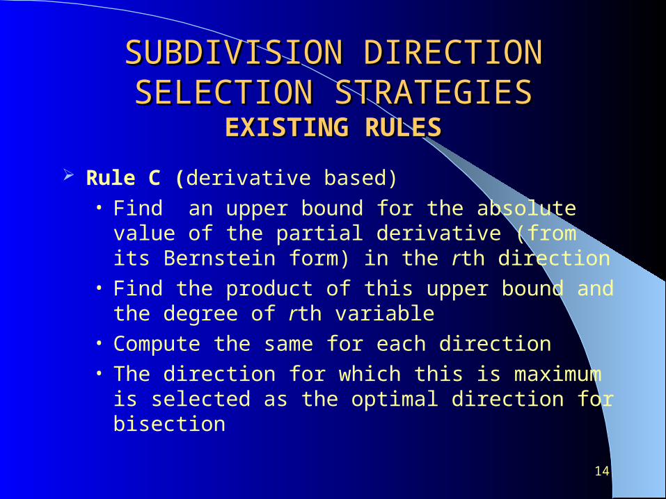
Rule C (derivative based)• Find an upper bound for the absolute value of the


• Find the product of this upper bound and the degree of rth variable



15


EXISTING RULESEXISTING RULES

Rule D (derivative based)• Find an upper bound for the absolute value of the


• Find the product of this upper bound and the edge length



16


EXISTING RULESEXISTING RULES Rule E (max width)

• Bisection is done along the component direction of maximal width

Rule F (randomized)• Pick a box randomly from the current list• Bisect it in all component directions• Find the maximal width of the polynomial over both these

boxes• Choose the component direction where this width is least

17

DISADVANTAGES OF THE DISADVANTAGES OF THE EXISTING METHODS OF EXISTING METHODS OF

BERNSTEIN COEFFICIENTS BERNSTEIN COEFFICIENTS COMPUTATIONSCOMPUTATIONS

Conventional method is very inefficient for higher dimensional polynomials

Even the Matrix multiplication method cannot be generalized to higher dimensional polynomials

18

DISADVANTAGES OF THE DISADVANTAGES OF THE EXISTING METHODS OF EXISTING METHODS OF BISECTION DIRECTION BISECTION DIRECTION

SELECTIONSELECTION

The existing rules generally need large computation times.

Certain existing rules are grossly inefficient, especially for higher dimensional polynomials.

19

DISADVANTAGES OF THE DISADVANTAGES OF THE EXISTING RANGE COMPUTATION EXISTING RANGE COMPUTATION

ALGORITHMSALGORITHMS

Fortran 95 can not readily cater to more than six dimensional arrays.

Bernstein coefficients generated are stored in multidimensional arrays

For getting sharp enclosures, subdivision usually creates large amount of data

All these are found to heavily slow down computations

20

NEW PROPOSITIONSNEW PROPOSITIONS

We propose new tools for

Bernstein Coefficient Computations Subdivision Direction Selection Acceleration devices

21

PROPOSITION 1PROPOSITION 1Computation of Bernstein CoefficientsComputation of Bernstein Coefficients

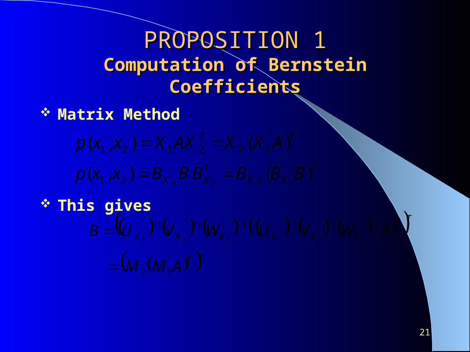
Matrix Method

This gives

TT AXXAXXxxp )(),( 122121 T

XXTXX BBBBBBxxp )(),(

121 221

TT

XXXXXX AWVUWVUB 111111

111222

TTAMM 12

22

PROPOSITION 1PROPOSITION 1Computation of Bernstein coefficientsComputation of Bernstein coefficients

Extending the above to trivariate case

where transpose means converting 3rd coordinate direction to 2nd , 2nd coordinate direction to 1st , 1st coordinate direction to 3rd

The same logic can be extended to the l-variate case

1111 111

XXX WVUM

1112 222

XXX WVUM

TTTAMMMB321123

23

PROPOSED MATRIX METHODPROPOSED MATRIX METHOD

For a 3-dimensional case instead of considering the polynomial coefficient matrix A as a 3 dimensional array, it can be considered as a matrix with 0 to n1 rows and 0 to (n2+1)(n3+1) –1 columns

After the third transpose and reshape the ‘A’ matrix would come in its original form

The same is shown as figures in the report.

24

Proposed Algorithm Proposed Algorithm Bernstein MatrixBernstein Matrix

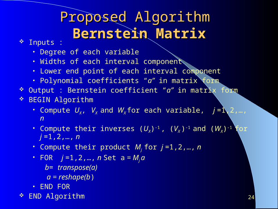
Inputs :• Degree of each variable • Widths of each interval component• Lower end point of each interval component • Polynomial coefficients “a” in matrix form

Output : Bernstein coefficient “a” in matrix form BEGIN Algorithm

• Compute UX, VX and WX for each variable, j =1,2,…, n• Compute their inverses (UX)-1

, (VX )-1 and (WX)-1 for j =1,2,…, n• Compute their product Mj for j =1,2,…, n• FOR j =1,2,…, n Set a = Mj a

b= transpose(a) a = reshape(b)

• END FOR END Algorithm

25

Comparison and results (Bernstein Comparison and results (Bernstein coefficients evaluation)coefficients evaluation)

Comparison is done between conventional method and the proposed Matrix method

All problems are taken from Verschelde’s PHC pack (database of polynomial systems)

Both methods generate the same Bernstein coefficients Proposed method gives results for all the examples Conventional method takes much longer time; it does not

give results for some examples even after a long time.

26

Time in seconds taken by the Matrix Time in seconds taken by the Matrix and the Conventional methods to and the Conventional methods to compute Bernstein coefficientscompute Bernstein coefficients

Ex Function Dim Domain t(Mat)

1 Lot Volt 3 [-1.5,2]3 0.000197

2 React Diff 3 [-5,5]3 0.00188

3 Lot Volt 4 [-2,2]4 0.00207

4 Capr sys 4 [-.5,.5]4 0.00213

5 Wright 5 [-5,5]5 0.00213

6 Reimer 5 5 [-1,1]5 0.02981

7 Mag 6 [-5,5]6 0.00345

8 Butcher 6 [-10,10]6 0.00285

9 Reimer 6 [-1,1]6 0.61231

10 Katsura 6 7 [-5,5]7 0.00741

11 Reimer 7 7 [-1,1]7 25.1991

t(Con)

0.00113

0.00098

0.00527

0.00722

0.00482

214.0184

0.51627

0.12679

*

3.65736

*

Ratio

0.5736

0.5213

2.5459

3.3897

2.2629

7179.4

149.64

44.48

>47,035

493.57

>1142.97

% Reduction

-74.33

-91.83

60.72

70.49

55.80

99.98

99.33

97.75

99.99

99.80

99.91

27

Some DefinitionsSome Definitions

Solution box is the box where ‘vertex property’ of the Bernstein coefficients is satisfied.

Solution patch is given by enclosure of the Bernstein coefficients over the solution box.

Current range is the hull of all solution patches.

28

PROPOSITIONPROPOSITION 2 2Subdivision Direction SelectionSubdivision Direction Selection

Proposed Rule 1 : Select patch with minimum hull

Find the patches with smallest and largest Bernstein coefficients from the entire list of patches

Find the respective distance of smallest and largest Bernstein coefficient to the infimum and supremum of the current range

Select that patch as the one which gives the largest distance, and bisect this selected patch in all component directions

29

EXAMPLEEXAMPLEDistanceDistance

Let a 3-d polynomial be given as

The polynomial coefficient and the Bernstein coefficient matrices are given as

Let at some stage the Current range be given by [1,20]

232

21

231

2332

21

3231212211

26

2542)(

xxxxxxxxx

xxxxxxxxxxp

2 ,1 ,2 321 nnn

20135.15.111211

5675.325.444

245.212

106005

010124

021012

BA

30

EXAMPLEEXAMPLE Let the two existing patches in the entire list be

Minimum and maximum value of Bernstein coefficients are 0.5 and 7.70 respectively

The respective distances are (1-0.5) = 0.5 and (20-7.70) = 12.30 Select the patch which has 7.70 as the Bernstein coefficient

625.78625.575.525.525.5

25.45.3625.2125.275.25.2

3225.15.5.12

70.725.7625.55.525.525.5

25.45625.2125.375.23

3425.125.12

31

Subdivision Direction SelectionSubdivision Direction Selection

Select patch with minimum hull

Hull of the Bernstein coefficients over both the generated subboxes is found out in each direction

The selected bisection direction is the one which gives the minimal hull.

32

PROPOSITION 3PROPOSITION 3Subdivision Direction SelectionSubdivision Direction Selection

Proposed Rule 2 : Randomized box with minimum hull Choose a box randomly from the current list.

The chosen box is bisected along each and every component direction.

Hull of the Bernstein coefficients over both the generated subboxes is found out in each direction.

The selected bisection direction is the one which gives the minimal hull.

33

RESULTS AND CONCLUSIONSRESULTS AND CONCLUSIONS Subdivision Direction SelectionSubdivision Direction Selection

All problems are taken from Verschelde’s PHC pack (database of polynomial systems)

Comparison of the bisection direction selection rules, on the basis of the following performance metrics • Number of solution boxes where vertex property/simplified vertex

condition is satisfied• Number of subdivisions• Maximum patch list length• Computation time in seconds

With the proposed rules we are able to solve all the examples

With rules A, B, C, D, E and F we are able to solve 90%, 70%, 70%, 50%, 90% and 90% of the examples, respectively

34


Comparison is done with all the existing rules (except rule D, which is unable to solve half the problems).

Proposed rules are found to be the most efficient, in terms of every performance metric

Reduction in number of solution boxes compared to Rule A is 82%, Rule B is 83%, Rule C is 83%, Rule E is 81% and Rule F is 84%

Reduction in number of subdivisions compared to Rule A is 84%, Rule B is 83%, Rule C is 83%, Rule E is 81% and Rule F is 84%

35


Reduction in the maximum list length compared to Rule A is 85%, Rule B is 51%, Rule C is 46%, Rule E is 34% and Rule F is 63%

Reduction in the computational time compared to Rule A is 98%, Rule B is 93%, Rule C is 93%, Rule E is 91% and Rule F is 93%

Both the rules give the same amount of reductions

36

PROPOSITION 4PROPOSITION 4Accelerating Devices for Range Accelerating Devices for Range

ComputationComputation Cut off test

Let the enclosure of Bernstein coefficients over a box be included in the current range.

This box can be deleted from further processing.

Any further subdivision of this box is not going to improve the current range.

Therefore, unnecessary subdivisions are eliminated

37


ComputationComputation Simplified Vertex Condition

Let smallest Bernstein coefficient in a patch appear at the vertex ; and the upper bound of this patch be included in the current range

This patch can be taken to be a solution patch

No further subdivision is required, as it would not give any further improvement in the current range

Same is true if the largest Bernstein coefficient in a patch is appearing at the vertex and the lower bound of the patch is included in the current range

38


ComputationComputation Monotonicity Test

If the polynomial is monotonic w.r.t any direction on a box

If the box is in the interior

• This box can be rejected If the box is not in the interior

• This box is retained

• No subdivision of this box in that direction

Avoids unnecessary subdivisions

39

PROPOSED ALGORITHMPROPOSED ALGORITHMRangeRange

Inputs : Maximum degree of each variable of the polynomial Coefficients of the polynomial in the form of a matrix Initial domain box Accuracy tolerances

Outputs: An enclosure of the range of the specified accuracy Number of solution boxes Number of subdivisions Maximum patch list length used to store the patches

40


BEGIN Algorithm Evaluate Bernstein coefficients in matrix form; put

them as a patch in a list. Set flags for simplified vertex condition, cut off test

and monotonicity test Take the first patch from the list and check for

‘vertex’/’simplified vertex’ condition.• If ‘true’, then update current range.• Else, perform ‘cut off test’.

• If list is not empty, choose a component direction based on a bisection rule

41


Take each patch from list, do the monotonicity test. If test is passed, proceed to next step; else discard tested box and choose next patch from the list.

Perform the necessary subdivision in the given direction and evaluate the new Bernstein coefficients

Update the list of patches and remove the tested box

Take the next patch from the list and perform the same operations, till the list is empty

Get the range of the polynomial from the current range END Algorithm

42

COMPARISON WITH COMPARISON WITH GLOBSOLGLOBSOL

We compare our results with the results obtained with Globsol

All problems are taken from Verschelde’s PHC pack, a database of polynomial systems.

Comparison of the computation time required by both the algorithms in terms of values of : Ratio Percent reduction

43

COMPARISON WITH COMPARISON WITH GLOBSOLGLOBSOL

Proposedby taken Time

Globsolby taken Time Ratio

100 timeGlobsol

timealgo proposed - timeGlobsol %reduction

44

Comparison of computation time by both Comparison of computation time by both the algorithmsthe algorithms

Ex. Test Function Dim Time, s Globsol Bernstein

1 Lotka 3 Number 0.0500 0.0049

Volterra Ratio 10.20

System % Reduction 90.20

2 Reaction 3 Number 0.0100 0.0101

Diffusion Ratio 0.9901

Problem % Reduction -1.0000

3 Lotka 4 Number 0.3500 0.0058

Volterra Ratio 60.3448

System 98.3429

4 Caprasse’s 4 Number 0.01 0.1940

System Ratio 1.9072

% Reduction 47.57

45

Ex. Test Function Dim Time, s Globsol Bernstein

5 System of

A.H. Wrightt

5 Number 0.01 0.0213

Ratio 0.4695

% Reduction -113.0000

6 System of

Reimer

5 Number 7.8300 4.3274

Ratio 1.8094

% Reduction 44.7300

7 Hunecke 5 Number 2.0300 2.7163

Ratio 0.7474

% Reduction -33.80

8 Cyclic

5-roots

Problem

5 Number * 0.0027

Ratio

% Reduction

9 Magnetism

In

Physics

6 Number 2.1700 1.9738

Ratio 1.0994

% Reduction 9.04

46

Ex. Test Function Dim. Time, s Globsol Bernstein

10 Camera 6 Number 2.24 0.1062

Displacement Ratio 21.0923

% Reduction 95.26

11 Butcher’s

Problem

6 Number 1.13 0.2072

Ratio 5.45054

% Reduction 81.6637

12 Hairer 6 Number 0.0200 0.0037

Ratio 5.4054

% Reduction 81.5000

13 System

Of

Reimer (6)

6 Number 1.2700 0.5885

Ratio 2.1580

% Reduction 53.6614

14 Magnetism

In

Physics

7 Number 5.0500 7.0464

Ratio 0.7167

% Reduction -39.533

47

Ex. Test Function Dim. Time, s Globsol Bernstein

15 Cyclic 7 Number 108.7500 0.1180

7-roots Ratio 921.6102

Problem % Reduction 99.8915

16 Heart

Dipole

Problem

8 Number 12.3500 1.1044

Ratio 11.1825

% Reduction 91.0575

17 Virasoro

Algebras

8 Number 222.7600 0.0039

Ratio 5.37e+04

% Reduction 99.9982

18 Cyclic

8-roots

Problem

8 Number 386.6000 0.0036

Ratio 1.07e+05

% Reduction 99.9991

48

RESULTSRESULTSComparison with GlobsolComparison with Globsol

In one of the examples Globsol was unable to give any result (arithmetic exception core dumped) indicated by ‘*’ in the table.

Compared to Globsol, the improved Bernstein method gives an average percent reduction in computational time of 47.38%

49

CONCLUSIONSCONCLUSIONS

The new algorithm Range is faster than Globsol in fourteen out of eighteen problems.

Further, on the average, we obtain considerable reductions in computation time with the proposed Algorithm Range.

50

FUTURE WORKFUTURE WORK

Modify the new algorithm after incorporating certain modifications in the Monotonicity test , thus further speeding up the algorithm Range

Integrate the code with COSY package of Berz et al.

Apply the method to Engineering problems, especially control engineering !

51

THANK YOU !THANK YOU !

Date post:	20-Dec-2015
Category:	Documents
View:	220 times
Download:	0 times

1 On Computing Ranges of Polynomials - Some Improvements to the Bernstein Approach P. S. V. Nataraj...

Documents