42
1 Pertemuan 13 Uji Koefisien Korelasi dan Regresi Matakuliah : A0392 – Statistik Ekonomi Tahun : 2006
| Date post: | 21-Dec-2015 |
| Category: |
Documents |
| View: | 222 times |
| Download: | 3 times |

1
Pertemuan 13Uji Koefisien Korelasi dan Regresi
Matakuliah : A0392 – Statistik Ekonomi
Tahun : 2006

2
Outline Materi : Uji koefisien korelasi Uji koefisien regresi Uji parameter intersep
3
Inference About The Slope and Coefficient Of Correlation
Inference about the slope with Analysis of Variance

4
Measures of Variation: The Sum of Squares
SST = SSR + SSE
Total Sample
Variability
= Explained Variability
+ Unexplained Variability

5
Measures of Variation: The Sum of Squares
• SST = Total Sum of Squares – Measures the variation of the Yi values
around their mean,
• SSR = Regression Sum of Squares – Explained variation attributable to the
relationship between X and Y
• SSE = Error Sum of Squares – Variation attributable to factors other than the
relationship between X and Y
(continued)
Y

6
Measures of Variation: The Sum of Squares
(continued)
Xi
Y
X
Y
SST = (Yi - Y)2
SSE =(Yi - Yi )2
SSR = (Yi - Y)2
_
_
_

7
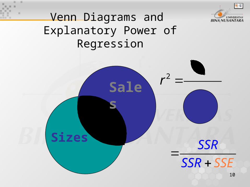
Venn Diagrams and Explanatory Power of Regression
Sales
Sizes
Variations in Sales explained by Sizes or variations in Sizes used in explaining variation in Sales
Variations in Sales explained by the error term or unexplained by Sizes
Variations in store Sizes not used in explaining variation in Sales
SSE
SSR
8
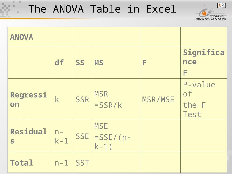
The ANOVA Table in Excel
ANOVA
df SS MS FSignificance
F
Regression
kSSR
MSR
=SSR/kMSR/MSE
P-value of
the F Test
Residualsn-k-1
SSE
MSE
=SSE/(n-k-1)
Total n-1SST

9
Measures of VariationThe Sum of Squares: Example
ANOVA
df SS MS F Significance F
Regression 1 30380456.12 30380456 81.17909 0.000281201
Residual 5 1871199.595 374239.92
Total 6 32251655.71
Excel Output for Produce Stores
SSR
SSERegression (explained) df
Degrees of freedom
Error (residual) df
Total df
SST
10
Venn Diagrams and Explanatory Power of Regression
Sales
Sizes
2
SSR
SSR S
r
SE
11
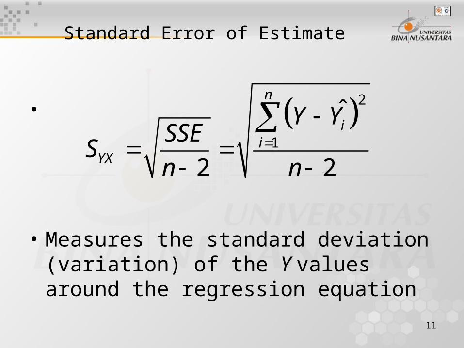
Standard Error of Estimate
•
• Measures the standard deviation (variation) of the Y values around the regression equation
2
1
ˆ
2 2
n
ii
YX
Y YSSE
Sn n

12
Measures of Variation: Produce Store Example
Regression StatisticsMultiple R 0.9705572R Square 0.94198129Adjusted R Square 0.93037754Standard Error 611.751517Observations 7
Excel Output for Produce Stores
r2 = .94
94% of the variation in annual sales can be explained by the variability in the size of the store as measured by square footage.
Syxn

13
Linear Regression Assumptions
• Normality– Y values are normally distributed for each X– Probability distribution of error is normal
• Homoscedasticity (Constant Variance)
• Independence of Errors

14
Consequences of Violationof the Assumptions
• Violation of the Assumptions– Non-normality (error not normally distributed)– Heteroscedasticity (variance not constant)
• Usually happens in cross-sectional data– Autocorrelation (errors are not independent)
• Usually happens in time-series data• Consequences of Any Violation of the Assumptions
– Predictions and estimations obtained from the sample regression line will not be accurate
– Hypothesis testing results will not be reliable• It is Important to Verify the Assumptions

15
• Y values are normally distributed around the regression line.
• For each X value, the “spread” or variance around the regression line is the same.
Variation of Errors Aroundthe Regression Line
X1
X2
X
Y
f(e)
Sample Regression Line
16
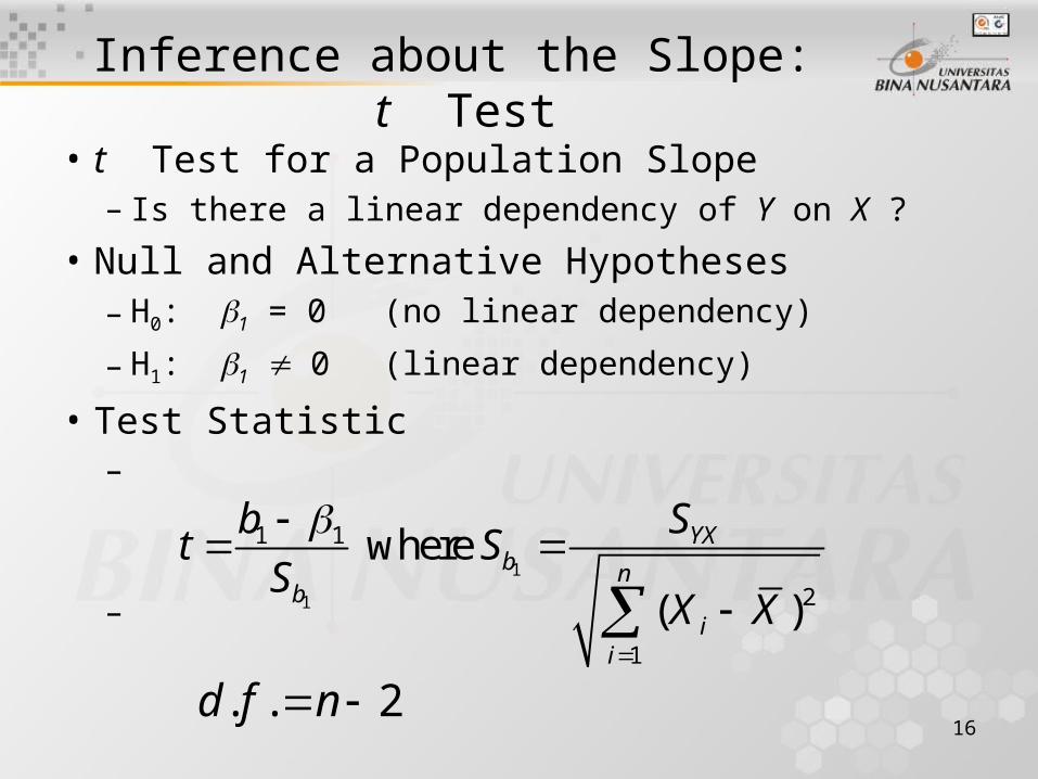
Inference about the Slope: t Test
• t Test for a Population Slope– Is there a linear dependency of Y on X ?
• Null and Alternative Hypotheses– H0: 1 = 0 (no linear dependency)
– H1: 1 0 (linear dependency)
• Test Statistic–
–
1
1
1 1
2
1
where
( )
YXb n
bi
i
b St S
SX X
. . 2d f n

17
Example: Produce Store
Data for 7 Stores:Estimated Regression Equation:Annual
Store Square Sales Feet ($000)
1 1,726 3,681
2 1,542 3,395
3 2,816 6,653
4 5,555 9,543
5 1,292 3,318
6 2,208 5,563
7 1,313 3,760
ˆ 1636.415 1.487i iY X
The slope of this model is 1.487.
Does square footage affect annual sales?

18
Inferences about the Slope: t Test Example
H0: 1 = 0
H1: 1 0
.05
df 7 - 2 = 5
Critical Value(s):
Test Statistic:
Decision:
Conclusion:There is evidence that square footage affects annual sales.
t0 2.5706-2.5706
.025
Reject Reject
.025
From Excel Printout
Reject H0.
Coefficients Standard Error t Stat P-valueIntercept 1636.4147 451.4953 3.6244 0.01515Footage 1.4866 0.1650 9.0099 0.00028
1b 1bS t
p-value
19
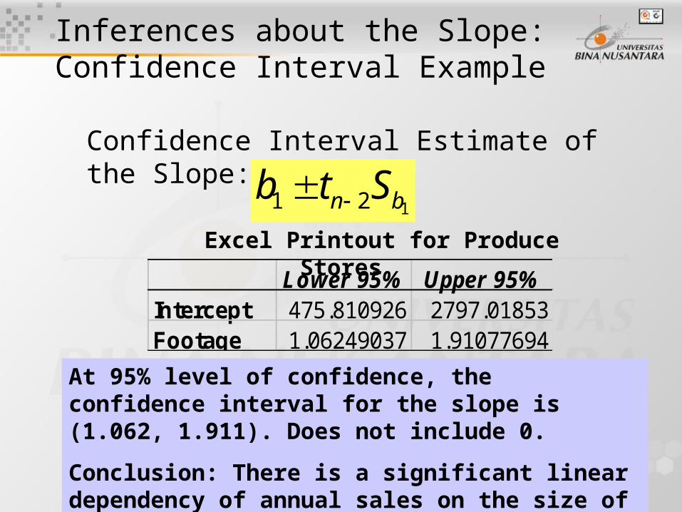
Inferences about the Slope: Confidence Interval Example
Confidence Interval Estimate of the Slope:
11 2n bb t S Excel Printout for Produce Stores
At 95% level of confidence, the confidence interval for the slope is (1.062, 1.911). Does not include 0.
Conclusion: There is a significant linear dependency of annual sales on the size of the store.
Lower 95% Upper 95%Intercept 475.810926 2797.01853Footage 1.06249037 1.91077694
20
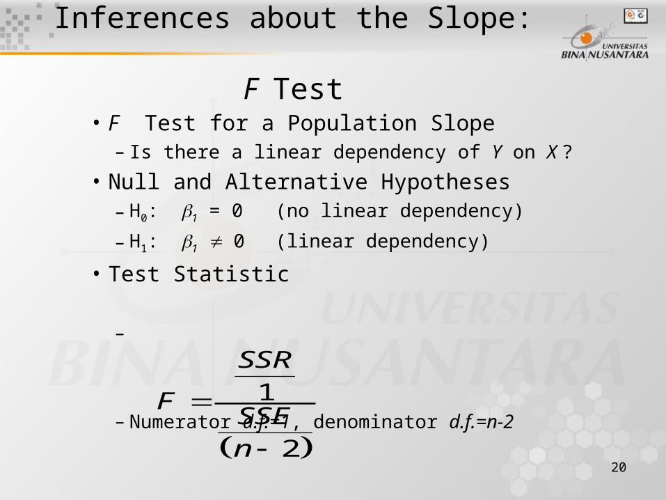
Inferences about the Slope: F Test
• F Test for a Population Slope– Is there a linear dependency of Y on X ?
• Null and Alternative Hypotheses– H0: 1 = 0 (no linear dependency)
– H1: 1 0 (linear dependency)
• Test Statistic
–
– Numerator d.f.=1, denominator d.f.=n-2
1
2
SSR
FSSEn
21
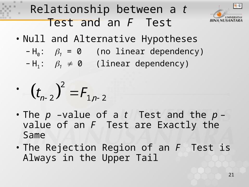
Relationship between a t Test and an F Test
• Null and Alternative Hypotheses– H0: 1 = 0 (no linear dependency)– H1: 1 0 (linear dependency)
•
• The p –value of a t Test and the p –value of an F Test are Exactly the Same
• The Rejection Region of an F Test is Always in the Upper Tail
2
2 1, 2n nt F
22
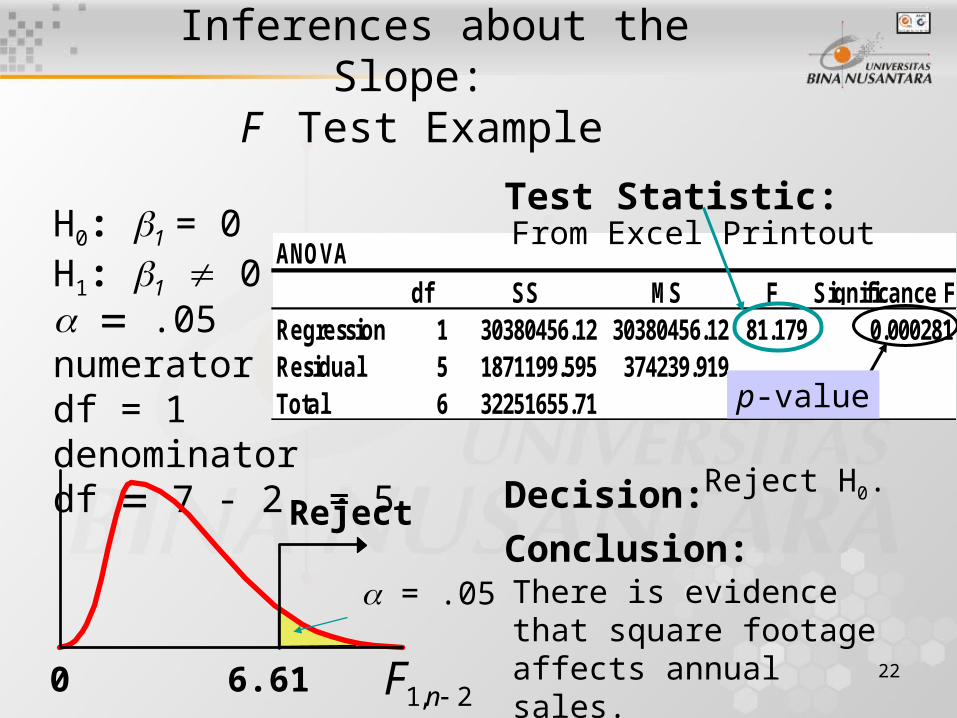
ANOVAdf SS MS F Significance F
Regression 1 30380456.12 30380456.12 81.179 0.000281Residual 5 1871199.595 374239.919Total 6 32251655.71
Inferences about the Slope: F Test Example
Test Statistic:
Decision:Conclusion:
H0: 1 = 0H1: 1 0 .05numerator df = 1denominator df 7 - 2 = 5
There is evidence that square footage affects annual sales.
From Excel Printout
Reject H0.
0 6.61
Reject
= .05
1, 2nF
p-value

23
Purpose of Correlation Analysis
• Correlation Analysis is Used to Measure Strength of Association (Linear Relationship) Between 2 Numerical Variables– Only strength of the relationship is concerned– No causal effect is implied

24
Purpose of Correlation Analysis
• Population Correlation Coefficient (Rho) is Used to Measure the Strength between the Variables
(continued)
XY
X Y

25
• Sample Correlation Coefficient r is an Estimate of and is Used to Measure the Strength of the Linear Relationship in the Sample Observations
Purpose of Correlation Analysis
(continued)
1
2 2
1 1
n
i ii
n n
i ii i
X X Y Yr
X X Y Y
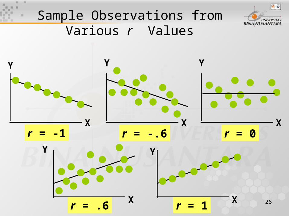
26r = .6 r = 1
Sample Observations from Various r Values
Y
X
Y
X
Y
X
Y
X
Y
X
r = -1 r = -.6 r = 0
27
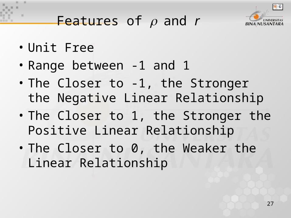
Features of and r
• Unit Free
• Range between -1 and 1
• The Closer to -1, the Stronger the Negative Linear Relationship
• The Closer to 1, the Stronger the Positive Linear Relationship
• The Closer to 0, the Weaker the Linear Relationship

28
• Hypotheses – H0: = 0 (no correlation)
– H1: 0 (correlation)
• Test Statistic
–
2
2 1
2 2
1 1
where
2n
i ii
n n
i ii i
rt
rn
X X Y Yr r
X X Y Y
t Test for Correlation
29
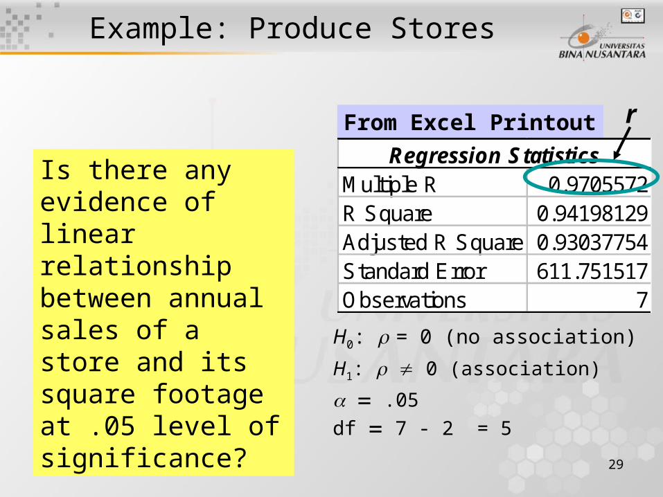
Example: Produce Stores
Regression StatisticsMultiple R 0.9705572R Square 0.94198129Adjusted R Square 0.93037754Standard Error 611.751517Observations 7
From Excel Printout r
Is there any evidence of linear relationship between annual sales of a store and its square footage at .05 level of significance?
H0: = 0 (no association)
H1: 0 (association)
.05
df 7 - 2 = 5

30
Example: Produce Stores Solution
0 2.5706-2.5706
.025
Reject Reject
.025
Critical Value(s):
Conclusion:There is evidence of a linear relationship at 5% level of significance.
Decision:Reject H0.
2
.97069.0099
1 .942052
rt
rn
The value of the t statistic is exactly the same as the t statistic value for test on the slope coefficient.
31
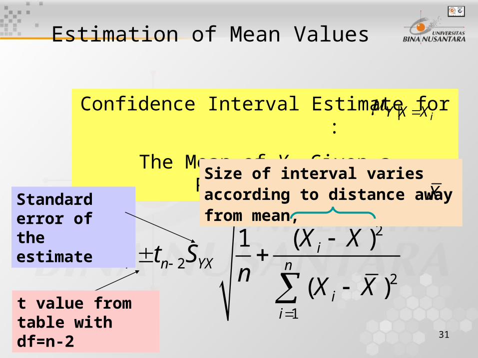
Estimation of Mean Values
Confidence Interval Estimate for :
The Mean of Y Given a Particular Xi
2
22
1
( )1ˆ
( )
ii n YX n
ii
X XY t S
n X X
t value from table with df=n-2
Standard error of the estimate
Size of interval varies according to distance away from mean, X
| iY X X

32
Prediction of Individual Values
Prediction Interval for Individual Response Yi at a Particular Xi
Addition of 1 increases width of interval from that for the mean of Y
2
22
1
( )1ˆ 1( )
ii n YX n
ii
X XY t S
n X X

33
Interval Estimates for Different Values of X
Y
X
Prediction Interval for a Individual Yi
a given X
Confidence Interval for the Mean of Y
Y i = b0 + b1X i
X
34
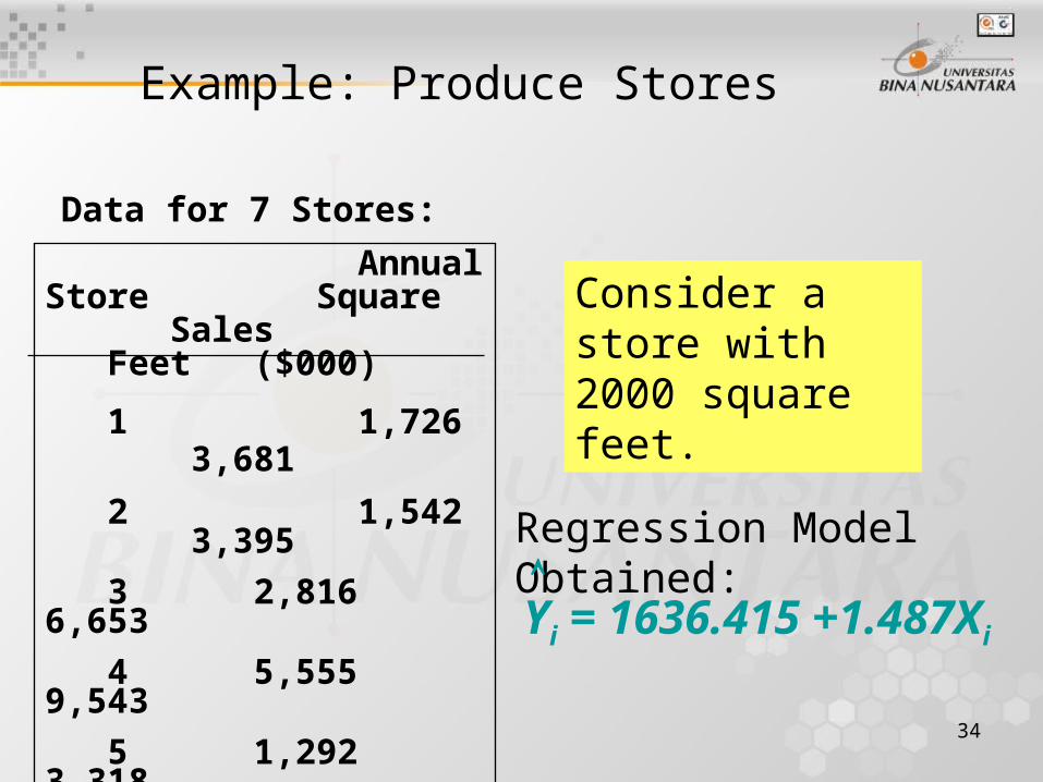
Example: Produce Stores
Yi = 1636.415 +1.487Xi
Data for 7 Stores:
Regression Model Obtained:
Annual Store Square Sales
Feet ($000)
1 1,726 3,681
2 1,542 3,395
3 2,816 6,653
4 5,555 9,543
5 1,292 3,318
6 2,208 5,563
7 1,313 3,760
Consider a store with 2000 square feet.

35
Estimation of Mean Values: Example
Find the 95% confidence interval for the average annual sales for stores of 2,000 square feet.
2
22
1
( )1ˆ 4610.45 612.66( )
ii n YX n
ii
X XY t S
n X X
Predicted Sales Yi = 1636.415 +1.487Xi = 4610.45 ($000)
X = 2350.29 SYX = 611.75 tn-2 = t5 = 2.5706
Confidence Interval Estimate for| iY X X
|3997.02 5222.34iY X X
36
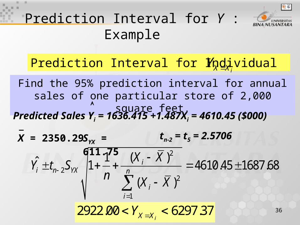
Prediction Interval for Y : Example
Find the 95% prediction interval for annual sales of one particular store of 2,000 square feet.
Predicted Sales Yi = 1636.415 +1.487Xi = 4610.45 ($000)
X = 2350.29 SYX = 611.75 tn-2 = t5 = 2.5706
2
22
1
( )1ˆ 1 4610.45 1687.68( )
ii n YX n
ii
X XY t S
n X X
Prediction Interval for Individual
2922.00 6297.37iX XY
iX XY

37
Estimation of Mean Values and Prediction of Individual Values in PHStat
• In Excel, use PHStat | Regression | Simple Linear Regression …– Check the “Confidence and Prediction Interval
for X=” box
• Excel Spreadsheet of Regression Sales on Footage
Microsoft Excel Worksheet

38
Pitfalls of Regression Analysis
• Lacking an Awareness of the Assumptions Underlining Least-Squares Regression
• Not Knowing How to Evaluate the Assumptions
• Not Knowing What the Alternatives to Least-Squares Regression are if a Particular Assumption is Violated
• Using a Regression Model Without Knowledge of the Subject Matter
39
Strategy for Avoiding the Pitfalls of Regression
• Start with a scatter plot of X on Y to observe possible relationship
• Perform residual analysis to check the assumptions
• Use a histogram, stem-and-leaf display, box-and-whisker plot, or normal probability plot of the residuals to uncover possible non-normality

40
Strategy for Avoiding the Pitfalls of Regression
• If there is violation of any assumption, use alternative methods (e.g., least absolute deviation regression or least median of squares regression) to least-squares regression or alternative least-squares models (e.g., curvilinear or multiple regression)
• If there is no evidence of assumption violation, then test for the significance of the regression coefficients and construct confidence intervals and prediction intervals
(continued)

41
Chapter Summary
• Introduced Types of Regression Models
• Discussed Determining the Simple Linear Regression Equation
• Described Measures of Variation
• Addressed Assumptions of Regression and Correlation
• Discussed Residual Analysis
• Addressed Measuring Autocorrelation

42
Chapter Summary
• Described Inference about the Slope
• Discussed Correlation - Measuring the Strength of the Association
• Addressed Estimation of Mean Values and Prediction of Individual Values
• Discussed Pitfalls in Regression and Ethical Issues
(continued)


