24
1 Tests of Hypotheses: Small Samples Chapter Rejection region
| Date post: | 19-Dec-2015 |
| Category: |
Documents |
| View: | 218 times |
| Download: | 0 times |

1
Tests of Hypotheses:
Small Samples
Tests of Hypotheses:
Small SamplesChapter
Rejectionregion

2CHAPTER GOALSCHAPTER GOALSTO DESCRIBE THE MAJOR
CHARACTERISTICS OF STUDENT’S t-DISTRIBUTION.
TO UNDERSTAND THE DIFFERENCE BETWEEN THE t -DISTRIBUTION AND THE z -DISTRIBUTION.
TO DESCRIBE THE MAJOR CHARACTERISTICS OF STUDENT’S t-DISTRIBUTION.
TO UNDERSTAND THE DIFFERENCE BETWEEN THE t -DISTRIBUTION AND THE z -DISTRIBUTION.

3CHAPTER GOALSCHAPTER GOALSTO TEST A HYPOTHESIS INVOLVING ONE
POPULATION MEAN.TO TEST A HYPOTHESIS INVOLVING THE
DIFFERENCE BETWEEN TWO POPULATION MEANS.
TO CONDUCT A TEST OF HYPOTHESIS FOR THE DIFFERENCE BETWEEN A SET OF PAIRED OBSERVATIONS.
TO TEST A HYPOTHESIS INVOLVING ONE POPULATION MEAN.
TO TEST A HYPOTHESIS INVOLVING THE DIFFERENCE BETWEEN TWO POPULATION MEANS.
TO CONDUCT A TEST OF HYPOTHESIS FOR THE DIFFERENCE BETWEEN A SET OF PAIRED OBSERVATIONS.

4The t-distribution has the following properties:It is continuous, bell shaped and symmetrical
about zero like the z-distribution.There is a family of t-distributions with mean of
zero but one for each sample size.The t-distribution is more spread out and flatter
at the center than the z-distribution, but approaches the z-distribution as the sample size gets larger.
The t-distribution has the following properties:It is continuous, bell shaped and symmetrical
about zero like the z-distribution.There is a family of t-distributions with mean of
zero but one for each sample size.The t-distribution is more spread out and flatter
at the center than the z-distribution, but approaches the z-distribution as the sample size gets larger.
CHARACTERISTICS OF STUDENT’S t-DISTRIBUTION
CHARACTERISTICS OF STUDENT’S t-DISTRIBUTION
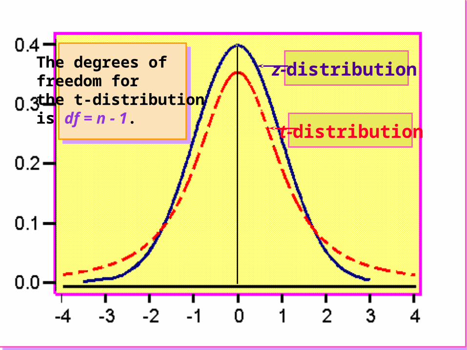
5z-distribution
t-distribution
The degrees of freedom forthe t-distribution is df = n - 1.

6A TEST FOR A POPULATION MEAN: SMALL SAMPLE, POPULATION
STANDARD DEVIATION UNKNOWN
A TEST FOR A POPULATION MEAN: SMALL SAMPLE, POPULATION
STANDARD DEVIATION UNKNOWN
The test statistic for a one sample case is given by equation (9-1) below
(9-1)
The test statistic for a one sample case is given by equation (9-1) below
(9-1) t X
nS
/
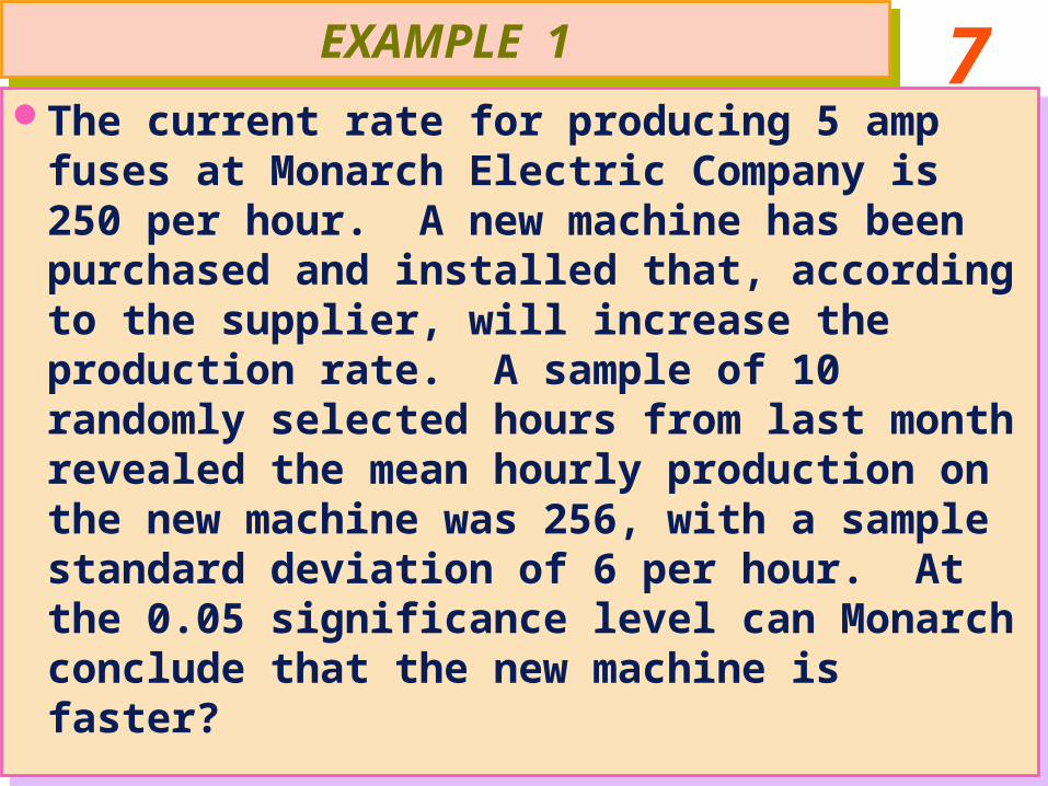
7The current rate for producing 5 amp fuses at
Monarch Electric Company is 250 per hour. A new machine has been purchased and installed that, according to the supplier, will increase the production rate. A sample of 10 randomly selected hours from last month revealed the mean hourly production on the new machine was 256, with a sample standard deviation of 6 per hour. At the 0.05 significance level can Monarch conclude that the new machine is faster?
The current rate for producing 5 amp fuses at Monarch Electric Company is 250 per hour. A new machine has been purchased and installed that, according to the supplier, will increase the production rate. A sample of 10 randomly selected hours from last month revealed the mean hourly production on the new machine was 256, with a sample standard deviation of 6 per hour. At the 0.05 significance level can Monarch conclude that the new machine is faster?
EXAMPLE 1EXAMPLE 1

8EXAMPLE 1 (continued)EXAMPLE 1 (continued)
Step 1: State the null and the alternative hypotheses.
H0: 250 H1: 250
Step 2: State the decision rule.H0 is rejected if t > 1.833, df = 9 (Appendix F).
Step 3: Compute the value of the test statistic.t = [256 - 250]/[6/10] = 3.16.Step 4: What is the decision on H0?
H0 is rejected. The new machine is faster.

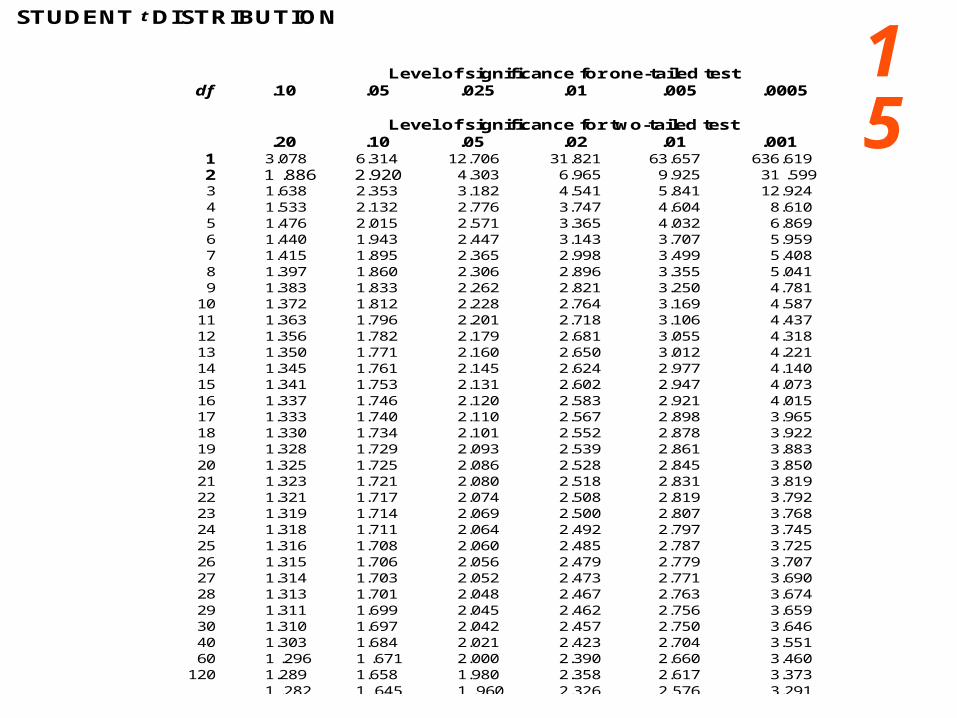
9STUDENT t DISTRIBUTION
Level of significance for one-tailed testdf .10 .05 .025 .01 .005 .0005
Level of significance for two-tailed test.20 .10 .05 .02 .01 .001
1 3.078 6.314 12.706 31.821 63.657 636.6192 1 .886 2.920 4.303 6.965 9.925 31 .5993 1.638 2.353 3.182 4.541 5.841 12.9244 1.533 2.132 2.776 3.747 4.604 8.6105 1.476 2.015 2.571 3.365 4.032 6.8696 1.440 1.943 2.447 3.143 3.707 5.9597 1.415 1.895 2.365 2.998 3.499 5.4088 1.397 1.860 2.306 2.896 3.355 5.0419 1.383 1.833 2.262 2.821 3.250 4.781
10 1.372 1.812 2.228 2.764 3.169 4.58711 1.363 1.796 2.201 2.718 3.106 4.43712 1.356 1.782 2.179 2.681 3.055 4.31813 1.350 1.771 2.160 2.650 3.012 4.22114 1.345 1.761 2.145 2.624 2.977 4.14015 1.341 1.753 2.131 2.602 2.947 4.07316 1.337 1.746 2.120 2.583 2.921 4.01517 1.333 1.740 2.110 2.567 2.898 3.96518 1.330 1.734 2.101 2.552 2.878 3.92219 1.328 1.729 2.093 2.539 2.861 3.88320 1.325 1.725 2.086 2.528 2.845 3.85021 1.323 1.721 2.080 2.518 2.831 3.81922 1.321 1.717 2.074 2.508 2.819 3.79223 1.319 1.714 2.069 2.500 2.807 3.76824 1.318 1.711 2.064 2.492 2.797 3.74525 1.316 1.708 2.060 2.485 2.787 3.72526 1.315 1.706 2.056 2.479 2.779 3.70727 1.314 1.703 2.052 2.473 2.771 3.69028 1.313 1.701 2.048 2.467 2.763 3.67429 1.311 1.699 2.045 2.462 2.756 3.65930 1.310 1.697 2.042 2.457 2.750 3.64640 1.303 1.684 2.021 2.423 2.704 3.55160 1 .296 1 .671 2.000 2.390 2.660 3.460
120 1.289 1.658 1.980 2.358 2.617 3.3731 .282 1 .645 1 .960 2.326 2.576 3.291

10Display of the Rejection Region, Critical Value, and the computed
Test Statistic
Display of the Rejection Region, Critical Value, and the computed
Test Statistic
Region ofrejection
t
Critical value1.833
0.05
df = 9
11To conduct this test, three assumptions are
required:
1. The populations must be normally or approximately normally distributed.
2. The populations must be independent.
3. The population variances must be equal.Let subscript 1 and 2 be associated with
population 1 and 2 respectively.
To conduct this test, three assumptions are required:
1. The populations must be normally or approximately normally distributed.
2. The populations must be independent.
3. The population variances must be equal.Let subscript 1 and 2 be associated with
population 1 and 2 respectively.
COMPARING TWO POPULATIONS MEANS
COMPARING TWO POPULATIONS MEANS
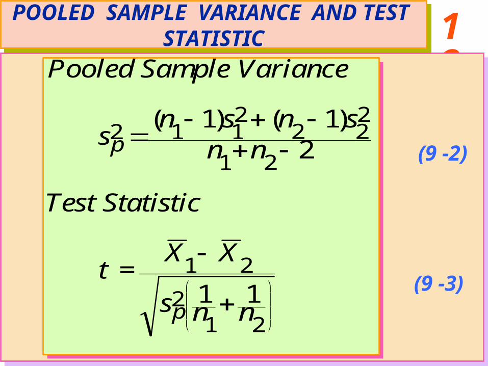
12POOLED SAMPLE VARIANCE AND TEST STATISTIC
POOLED SAMPLE VARIANCE AND TEST STATISTIC
Pooled Sample Variance
sn s n s
n n
Test Statistic
tX X
s n n
p
p
=
1
2 1 12
2 22
1 2
2
21 2
1 12
1 1
( ) ( )
(9 -3)
(9 -2)

13EXAMPLE 2EXAMPLE 2
A recent Environmental Protection Agency (EPA) study compared the highway fuel economy of domestic and imported passengers cars. A sample of 15 domestic cars revealed a mean of 33.7 mpg with a standard deviation of 2.4 mpg. A sample of 12 imported cars revealed a mean of 35.7 mpg with a standard deviation of 3.9. At the 0.05 significance level can the EPA conclude that the miles per gallon is higher on the imported cars? (Let subscript 1 be associated with the domestic cars).
A recent Environmental Protection Agency (EPA) study compared the highway fuel economy of domestic and imported passengers cars. A sample of 15 domestic cars revealed a mean of 33.7 mpg with a standard deviation of 2.4 mpg. A sample of 12 imported cars revealed a mean of 35.7 mpg with a standard deviation of 3.9. At the 0.05 significance level can the EPA conclude that the miles per gallon is higher on the imported cars? (Let subscript 1 be associated with the domestic cars).

14Step 1: State the null and the alternative
hypotheses.H0: H1:
Step 2: State the decision rule.H0 is rejected if t > 1.708, df = 25.
Step 3: Compute the value of the test statistic.t = 1.64 (Verify).Step 4: What is the decision on H0?
H0 is not rejected. Insufficient sample evidence to claim a higher mpg on the imported cars.
Step 1: State the null and the alternative hypotheses.
H0: H1:
Step 2: State the decision rule.H0 is rejected if t > 1.708, df = 25.
Step 3: Compute the value of the test statistic.t = 1.64 (Verify).Step 4: What is the decision on H0?
H0 is not rejected. Insufficient sample evidence to claim a higher mpg on the imported cars.
EXAMPLE 2 (continued)EXAMPLE 2 (continued)
15STUDENT t DISTRIBUTION
Level of significance for one-tailed testdf .10 .05 .025 .01 .005 .0005
Level of significance for two-tailed test.20 .10 .05 .02 .01 .001
1 3.078 6.314 12.706 31.821 63.657 636.6192 1 .886 2.920 4.303 6.965 9.925 31 .5993 1.638 2.353 3.182 4.541 5.841 12.9244 1.533 2.132 2.776 3.747 4.604 8.6105 1.476 2.015 2.571 3.365 4.032 6.8696 1.440 1.943 2.447 3.143 3.707 5.9597 1.415 1.895 2.365 2.998 3.499 5.4088 1.397 1.860 2.306 2.896 3.355 5.0419 1.383 1.833 2.262 2.821 3.250 4.781
10 1.372 1.812 2.228 2.764 3.169 4.58711 1.363 1.796 2.201 2.718 3.106 4.43712 1.356 1.782 2.179 2.681 3.055 4.31813 1.350 1.771 2.160 2.650 3.012 4.22114 1.345 1.761 2.145 2.624 2.977 4.14015 1.341 1.753 2.131 2.602 2.947 4.07316 1.337 1.746 2.120 2.583 2.921 4.01517 1.333 1.740 2.110 2.567 2.898 3.96518 1.330 1.734 2.101 2.552 2.878 3.92219 1.328 1.729 2.093 2.539 2.861 3.88320 1.325 1.725 2.086 2.528 2.845 3.85021 1.323 1.721 2.080 2.518 2.831 3.81922 1.321 1.717 2.074 2.508 2.819 3.79223 1.319 1.714 2.069 2.500 2.807 3.76824 1.318 1.711 2.064 2.492 2.797 3.74525 1.316 1.708 2.060 2.485 2.787 3.72526 1.315 1.706 2.056 2.479 2.779 3.70727 1.314 1.703 2.052 2.473 2.771 3.69028 1.313 1.701 2.048 2.467 2.763 3.67429 1.311 1.699 2.045 2.462 2.756 3.65930 1.310 1.697 2.042 2.457 2.750 3.64640 1.303 1.684 2.021 2.423 2.704 3.55160 1 .296 1 .671 2.000 2.390 2.660 3.460
120 1.289 1.658 1.980 2.358 2.617 3.3731 .282 1 .645 1 .960 2.326 2.576 3.291
16Sampling Distribution for the Statistic t for a Two-Tailed Test, 0.05 Level of
Significance
Sampling Distribution for the Statistic t for a Two-Tailed Test, 0.05 Level of
Significance
Criticalvalue2.06
Criticalvalue-2.06
0.95
Do notreject H0
Region ofrejectionRegion of
rejection
0.025 0.025
t-2.06 2.06
df = 25
0

17Use the following test when the samples are
dependent. For example, suppose you were collecting data
on the price charged by two different body shops because you suspect that one is charging more than the other.
In this case, the same wrecked vehicle will be assessed by the two shops.
Because of this, the samples will be dependent.Here we will take the difference of the two
estimates and perform a test on the differences.
Use the following test when the samples are dependent.
For example, suppose you were collecting data on the price charged by two different body shops because you suspect that one is charging more than the other.
In this case, the same wrecked vehicle will be assessed by the two shops.
Because of this, the samples will be dependent.Here we will take the difference of the two
estimates and perform a test on the differences.
HYPOTHESIS TESTING INVOLVING PAIRED OBSERVATIONS
HYPOTHESIS TESTING INVOLVING PAIRED OBSERVATIONS

18TEST STATISTICTEST STATISTIC
(9 - 4) (9 - 4)
d-bar is the average of the differences
sd is the standard deviation of the differences
n is the number of pairs (differences)
t ds nd
/

19An independent testing agency is comparing the
daily rental cost for renting a compact car from Hertz and Avis. A random sample of eight cities is obtained and the following rental information obtained. At the 0.05 significance level can the testing agency conclude that there is a difference in the rental charged?
NOTE: These samples are dependent since the same type of car (compact) is being rented from the two companies in the same cities.
An independent testing agency is comparing the daily rental cost for renting a compact car from Hertz and Avis. A random sample of eight cities is obtained and the following rental information obtained. At the 0.05 significance level can the testing agency conclude that there is a difference in the rental charged?
NOTE: These samples are dependent since the same type of car (compact) is being rented from the two companies in the same cities.
EXAMPLE 3EXAMPLE 3

20
EXAMPLE 3 (continued)EXAMPLE 3 (continued)
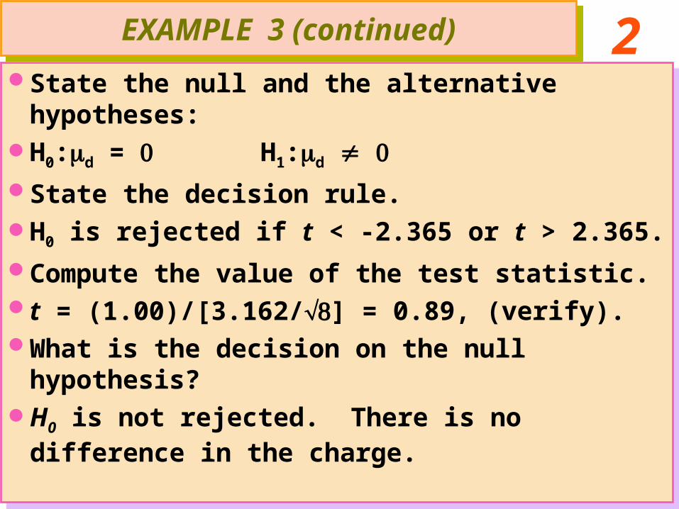
21State the null and the alternative hypotheses:H0:d = H1:d
State the decision rule.H0 is rejected if t < -2.365 or t > 2.365.
Compute the value of the test statistic.t = (1.00)/[3.162/] = 0.89, (verify).What is the decision on the null hypothesis?H0 is not rejected. There is no difference in the
charge.
State the null and the alternative hypotheses:H0:d = H1:d
State the decision rule.H0 is rejected if t < -2.365 or t > 2.365.
Compute the value of the test statistic.t = (1.00)/[3.162/] = 0.89, (verify).What is the decision on the null hypothesis?H0 is not rejected. There is no difference in the
charge.
EXAMPLE 3 (continued)EXAMPLE 3 (continued)

22STUDENT t DISTRIBUTION
Level of significance for one-tailed testdf .10 .05 .025 .01 .005 .0005
Level of significance for two-tailed test.20 .10 .05 .02 .01 .001
1 3.078 6.314 12.706 31.821 63.657 636.6192 1 .886 2.920 4.303 6.965 9.925 31 .5993 1.638 2.353 3.182 4.541 5.841 12.9244 1.533 2.132 2.776 3.747 4.604 8.6105 1.476 2.015 2.571 3.365 4.032 6.8696 1.440 1.943 2.447 3.143 3.707 5.9597 1.415 1.895 2.365 2.998 3.499 5.4088 1.397 1.860 2.306 2.896 3.355 5.0419 1.383 1.833 2.262 2.821 3.250 4.781
10 1.372 1.812 2.228 2.764 3.169 4.58711 1.363 1.796 2.201 2.718 3.106 4.43712 1.356 1.782 2.179 2.681 3.055 4.31813 1.350 1.771 2.160 2.650 3.012 4.22114 1.345 1.761 2.145 2.624 2.977 4.14015 1.341 1.753 2.131 2.602 2.947 4.07316 1.337 1.746 2.120 2.583 2.921 4.01517 1.333 1.740 2.110 2.567 2.898 3.96518 1.330 1.734 2.101 2.552 2.878 3.92219 1.328 1.729 2.093 2.539 2.861 3.88320 1.325 1.725 2.086 2.528 2.845 3.85021 1.323 1.721 2.080 2.518 2.831 3.81922 1.321 1.717 2.074 2.508 2.819 3.79223 1.319 1.714 2.069 2.500 2.807 3.76824 1.318 1.711 2.064 2.492 2.797 3.74525 1.316 1.708 2.060 2.485 2.787 3.72526 1.315 1.706 2.056 2.479 2.779 3.70727 1.314 1.703 2.052 2.473 2.771 3.69028 1.313 1.701 2.048 2.467 2.763 3.67429 1.311 1.699 2.045 2.462 2.756 3.65930 1.310 1.697 2.042 2.457 2.750 3.64640 1.303 1.684 2.021 2.423 2.704 3.55160 1 .296 1 .671 2.000 2.390 2.660 3.460
120 1.289 1.658 1.980 2.358 2.617 3.3731 .282 1 .645 1 .960 2.326 2.576 3.291

23
2.3650
Computedt = 0.89
Rejectionregion
-2.365
Rejectionregion
0.89
df = 7
t

24
Chapter 11 : CD-ROM
Chapter 12 : CD-ROM
Chapter 13 : CD-ROM
Chapter 11 : CD-ROM
Chapter 12 : CD-ROM
Chapter 13 : CD-ROM
Homework for Chapter 11,12,13 Homework for Chapter 11,12,13


