The Economic Origins of Democracy Reconsidered

John R. Freeman

University of Minnesota

Dennis P. Quinn

Georgetown University

10 November 2009 (v4)

Draft – comments welcome

The first version of this paper was presented at the Annual Meeting of the American Political Science Association, Boston, August 28, 2008. A later version was presented at Yale University in November of that same year. We thank James Galbraith, Irfan Nooruddin, Keith Ord, Pietra Rivoli, Thomas Sattler, Ken Scheve, and Vineeta Yadav for comments and suggestions. The paper also benefited from comments at a presentation at the Political Economy working group series at Georgetown. The authors thank Rebecca Anderson, Naphat Kissamrej, Dafina Nikolova, Erica Owen, and Ravi Tayal for excellent research assistance. We thank Aart Kraay for discussions of the inequality data sets available, and Keith Ord for advice on the research design. Sections of this paper draw on work done jointly in other projects with Manmohan Kumar, A. Maria Toyoda, and Hans-Joachim Voth.

2

ABSTRACT

The effect of economic changes sparked by globalization on democracy and

autocracy is a central research question in the social sciences. We review the prevailing

arguments about the links among inequality, financial integration and democratization,

focusing in particular on the contributions of Acemoglu and Robinson (2006) and Boix

(2003). In contrast to the arguments of these scholars, we argue that, because financial

liberalization produces increases in income inequality and allows for capital taxation, in

financially open economies, the relationship between income inequality and

democratization is a “U.” Countries with lower and higher levels of income inequality

are more likely to democratize once they open their economies financially. Our test

employs the most current and reliable income inequality and financial globalization

measures available. We employ a design suggested by Acemoglu, Johnson, Robinson,

Yared (2008). Given financial closure, we find some support for Acemoglu and

Robinson’s main causal claims. Given international financial openness, rather than the

hump-shape predicted by Acemoglu and Robinson or the step change from democracy to

autocracy predicted by Boix (2003), we find a U-shaped pattern between these inequality

and democratization. (182 words)

3

Much has been written in recent years about the positive connection between the

“third wave” of democratization and economic globalization. The fact that these

developments are occurring simultaneously leads many scholars and commentators to

suggest a connection between democratization and some forms of economic

globalization. For example, numerous studies find that democracies liberalize trade, and

that trade appears to reinforce democracy. An example is Eichengreen and Leblang

(2008). Using a design that covers a relatively long period of time and multiple measures

of globalization, Eichengreen and Leblang find a positive relationship between

democracy and trade openness. Similar findings are reported by Milner and Mukherjee

(2009). Figure 1 shows data for the global averages over time for several indicators of

democracy and indicators of trade and capital account openness (described below). It

appears from the figure that democracy and economic globalization indeed are closely

related phenomena.

At the same time, researchers recognize several lacunas in the literature. One is

theoretical. Milner and Mukherjee argue that we lack convincing “detailed causal

theories” to explain the positive correlation between economic globalization and

democracy. A second lacuna is the relative lack of studies of the effects of financial

globalization on democratization.

The economic origins of democracy literature offers another perspective on

economic globalization and democracy. In this genre, income inequality and the nature of

capital—the relative share of land to physical capital and, relatedly, the specificity of

capital are key variables. Acemoglu and Robinson (2006) argue that, because of the

threat of redistribution, income inequality and democracy have a complex relationship,

4

namely, it is hump shaped (an inverse U). Boix (2003), in contrast, contends that

democratization depends on the interrelationship of income inequality and asset

specificity. For instance, for a high level of asset specificity, income inequality reduces

the likelihood of democratization. If asset specificity is low, the prospects for

democratization are much brighter.

This research and the literature on economic globalization are not well integrated.

Scholars differ in how they incorporate economic globalization, especially financial

globalization, in their models. Acemoglu and Robinson (2006: Chapter 9 and 10)

explicitly extend their model to allow elites to own land and to open their economy trade

and capital flows. But these extensions leave their principle result—the hump shaped

relationship between inequality and democracy intact. The effects of economic

globalization are more implicit in Boix (2003). Boix makes only passing reference to the

effect that economic openness has on asset specificity; he suggests that financial

liberalization generally reduces asset specificity but does not explain how this occurs. He

also does not supply an analysis of the effect of openness on inequality. In general

scholars studying the economic origins of democracy make little or no mention of the

closed-open economy distinction. The same is true of scholars who recently tested the

causal claims in the economics origins of democracy literature; no variables for economic

openness are included as controls in their models. They also make no attempt to link their

periodizations—embodied in temporal dummies—to changes in levels of economic

openness (Houle 2009; see also the test in Ansell and Samuels, 2009).1

1 Houle (2009) includes land and trade openness in his multiple imputation model but not in his explanatory model. The only variable in his explanatory model remotely related to openness is oil exportation and this is included to capture arguments about natural resource politics. As regards the changing degree of economic globalization over time, Houle checks for robustness in his dynamic probit model with decade

5

We focus here on the effects of financial globalization on democracy. We

synthesize the literatures on democracy and globalization and on the economic origins of

democracy. We concur that income inequality and asset specificity are key elements of

the causal nexus that produces the correlation between economic globalization and

democracy. But we argue that the relationship between these variables and democracy

differs fundamentally in closed and open economies. In particular, the extensive financial

liberalization in conjunction with recent financial innovations like deposit receipts and

the persistence of capital income taxation means the causal chain connecting income

inequality and asset specificity to democracy is reversed in open economies. For

example, what is a “hump shape” relationship in the closed case becomes a U shape

relationship in the open economies. It follows that tests of causal theories about the links

between income inequality, asset specificity, and democracy must include measures of

financial openness and (or) they must be performed separately for periods in which the

degree (type) of financial and other kinds of globalization varied. We perform the first

test for such a reversal in the causal relationships between these variables here.

Our paper is divided into four parts. Part one reviews the major works that bear

on the relationship between economic globalization and democracy as well as recent

attempts to test their causal claims.2 Our new theory for why the relationship between

economic globalization—especially financial globalization—and democracy reverses is

presented in section two. This theory builds on the work of Acemoglu and Robinson and

and regional dummy variables. But he draws no implications from these dummies about changes in economic openness. Eichengreen and Leblang (2008) actually find that financial liberalization does not have a causal impact on democracy in their “post WWII subperiod.” However this subperiod covers four decades when economies were both closed and open. We critique these and other tests of the two literatures in the first section of our paper. 2This paper analyzes democratization. Democratic consolidation is left to a future work.

6

Boix, but also incorporates the newest developments in international finance such as the

ability of land owners to reduce asset specificity through American and Global Deposit

Receipts (ADRs and GDRs, respectively). Our theory is tested in the third section. Our

test employs new data for inward and outward capital account restrictions, and updated

inequality indicators. Our inferences are based on dynamic panel models; we estimate

this model with both OLS and the system Generalized Method of Moments (system

GMM). The results confirm our predicted pattern of a U relationship between inequality

and democracy in a financially open world. Economic globalization reverses in

significant ways the relationships between variables like income inequality and

democracy.

Literature Review

The Economic Determinants of Democracy in Closed Economies3

The arguments of AR and Boix are similar, though their conclusions differ. AR

explain the economic origins of democracy in terms of the politics of income inequality;

this argument follows from an analysis of their “workhorse model.” As we explain

below, capital and land are introduced later as an extension of this model AR partition

society into two groups, the poor and the rich (p, r), an architecture that Boix (2003) also

adopts (following earlier work by AR and others) .4 The poor outnumber the rich by a

3 In this paper, we focus on the two most prominent published works in this literature, Acemoglu and Robinson (2006) and Boix (2003). We also focus on the main models in these works, the two actor models that analyze the negotiations between the poor and the rich. Future work will analyze the more complex, three actor models that introduce a middle class as well as newer, unpublished models of this kind (Ansell and Samuels 2009). 4 See AR 2006, p. 87 for a discussion of the relationship of their work to Boix’s, and see Boix 2003, p. 11, for a discussion of the relationship of his work to theirs.

7

considerable margin.5 The two groups have complete information. They struggle over the

distribution of resources; redistribution is accomplished by means of a common

proportional tax, the proceeds of which are transferred (in equal shares) to all members of

society. Democracy is an institution that makes commitments to redistribution more

credible than the promises to redistribute by the rich (in autocracy). The questions are: 1)

Do the poor accept the policies and promises offered by the rich or do they choose to

revolt?; and, concomitantly, 2) Do the rich offer tax rates that are their most preferred

policy (zero taxation), “concessionary” rates that are nonzero but also not the rates most

preferred by the poor, or choose to democratize?

AR and Boix use game theory to derive the best responses (strategies) of the rich

and poor under a variety of conditions pertaining to democratic and autocratic societies.

Their accounts of democracy are based on previous work by Meltzer and Richard (1981)

and others. The core idea is that in democracy the median voter is a poor individual

whose preferences on tax policy are always determinative.

In the AR model, the median voter’s preference takes into account the deadweight

loss of taxation, C(τ). But, even then, unlike the rich, the median voter still favors a

nonzero tax rate, τp. Moreover, her preferred tax rate increases with the level of

inequality in society; mathematically, this follows from the assumption that the share of

income held by the rich, θ, is greater than the share of the population that is poor, δ.

5 In several places in their book AR consider more complex partitioning of society, including the possibility of a middle class. But their core argument is framed in terms of a distributional struggle between the poor and the rich.

8

Therefore, in democracy, the median voter’s preferences are always implemented and

this leaves the poor better off and the rich worse off in terms of post-tax income.6

The situation in autocracy is a bit more complicated. AR’s workhorse model

implies that the rich have a choice between imposing a tax rate that, from their point of

view, is no better than τp or risk suffering a revolution and losing all their wealth. For

their part, the poor must choose between accepting the tax rate imposed by the rich or

opting for revolution. A key assumption regarding the latter option is that revolutions

destroy forever a share of societal resources, µ. This means that, after the revolution,

while the rich have no income, the poor earn a reduced rate than what would be possible

in a democracy, were the preferences of the (poor) median voter to be adopted.7 So, for

the poor, the question, in the simplest static model, is whether their post tax income is

higher under the tax rate offered them by the autocratic rich relative to the post tax

income they would obtain after losing a share of societal resources in the revolution. AR

call this the revolutionary constraint. They show it is equivalent to the condition θ> µ.8

Democratization occurs when revolution is relatively more attractive to the poor

than the concessions the rich might offer and, for the rich, repression is more costly than

democratization.9 Given these results, AR then show that democratization is likely only

6Pre tax incomes of the two groups are expressed as yp = [(1-θ) /(1-δ)] and yr = (θ )/δ where θ is the share of the income accruing to the rich, δ is the fraction of the population that is rich (assumed to be less than .50), and is the average income of individuals in the society. Post tax income is expressed as V(yi | τ) = (1 – τ) yi + T = (1 – τ)yi + (τ – C(τ)) where V denotes indirect utility, yi is the income of individual i, τ is the tax rate, T is the transfer (from government collected taxes), C(τ) is the deadweight loss of taxation, and is defined as before. AR show that the derivative of τp with respect to the level of inequality in society, θ, is positive. 7 That is, after revolution the payoff to the rich, Vr(R,µ) = 0 and the payoff to the poor is Vp(R,µ)= [(1-µ) ]/(1-δ) where µ is the share resources destroyed forever by the revolution, is average societal income and δ is the share of the population that is poor. 8 This derives from the condition Vp(R,µ) > yp. 9See Proposition 6.2, AR p. 189.

9

under intermediate levels of inequality, θ. For low levels of θ, revolution is not a viable

option for the poor. Hence, the rich may be able to implement their most preferred tax

policy and; therefore, autocracy survives. Above a certain high threshold level of θ, elites

have more to lose from democracy than they do from repression (or from concessions).

The rich, therefore, opt for repression and all agents suffer a loss in income. But this

leaves the rich relatively better off than they would be if they agreed to democracy and

the poor were able to choose their most preferred tax policy.10

AR thus propose the following causal proposition:

AR Proposition 1. In closed economies there is a (convex) hump-shaped relationship between societal inequality and democratization within and across countries.

As regards capital, in an extension of their “workhorse model” for the closed

economy, AR let production depend on both land and the capital stock. The poor earn

wages while the rich earn rent from land and returns from capital. Markets are assumed to

be perfectly competitive so these earnings (returns) equal their marginal products. The

key political parameters are the relative cost of repression (revolution) on the types of

capital and the capital-to-land ratio. When the cost to capital from repression (revolution)

is greater than the cost to land and the capital-to-land ratio is greater than a certain

10This is AR’s Corollary 6.1. To derive this key corollary, AR examine the conditions relative to θ, that (the promise of) concessionary taxation is just enough to prevent revolution, the condition relative to θ under which the value of democracy is equal to that of revolution for the poor. They show there is a range of inequality levels where democracy can be conceded by the rich, the rich end up better off than if they had repressed (given the value of the cost of repression) and the poor do are satisfied with the tax policy of the median voter. There is, however, an upper threshold in equality that produces democracy, however. Beyond this upper threshold, democracy—the tax policy of the median (poor) voter—leaves the rich worse off than they would be under repression. Put another way, at this upper level of inequality, the cost of repression has to be very high before the rich would opt for democratization. At this upper level, either a) (promises of) concessionary taxation don’t work, the poor prefer revolution, and repression is the only option for the rich (to avoid a total loss of income) or b) the poor prefer democracy to revolution, but the rich still are better off repressing the poor than agreeing to democracy and accruing the post-tax income produced by the tax policy of the median (poor) voter, τp.

10

threshold, the rich always choose democracy over repression. Put another way, “capital

investments make the elites more prodemocratic than land holdings” (2003, p. 296). In

this way, AR rationalize the findings of Barrington Moore and others about the relative

likelihood of autocracy in agrarian societies.11

Boix (2003) argues that the origins of democracy depend on both inequality and

asset specificity. The distinction between closed and open economies is implicit in the

general model he develops. As noted above, Boix also partitions society into the poor and

the wealthy. Each group owns some share of a country’s capital. Each group’s income is

a function of this capital. But the wealthy sometimes can earn income abroad. How much

income the wealthy can earn abroad depends on the specificity of their capital. Formally,

ya = k(1-σ) where ya is this foreign income, k is capital and σ is a parameter that is 1

when capital is purely specific—Boix gives land as an example—and 0 when capital is

completely mobile. We will call this the asset specificity constraint. It embodies the

possibility of the wealthy augmenting their income from foreign investment.12

In the Boix model, each group’s utility is simple a linear function of their

members expected income minus the costs associated with different kinds of governance.

In democracy, the government tax level, τ, as in the AR set-up, is chosen by a member of

the poor, more specifically, the (poor) median voter. This (poor) median voter maximizes

11See AR’s Corrollary 9.1 in section 9.2 12 The concept of asset specificity is central to Boix’s argument. The “specificity” of an asset for Boix depends on its value outside the country of origin:…”capital can be thought of as being somewhat specific to the country in which it is being used. The extent to which an asset is specific is measured by its productivity at home relative to its productivity abroad. Whenever capital is moved abroad, it loses a share (σ) of its value. More exactly, capital k, which at home would produce y = k, produces abroad ya = k(1- σ). Thus, the more specific the capital, that is the larger the σ, the less attractive the option of moving capital abroad becomes to its owners. The degree of specificity varies across types of capital: it is practically complete for land, yet extremely low for money or generic skills (2003, 22-23).”

11

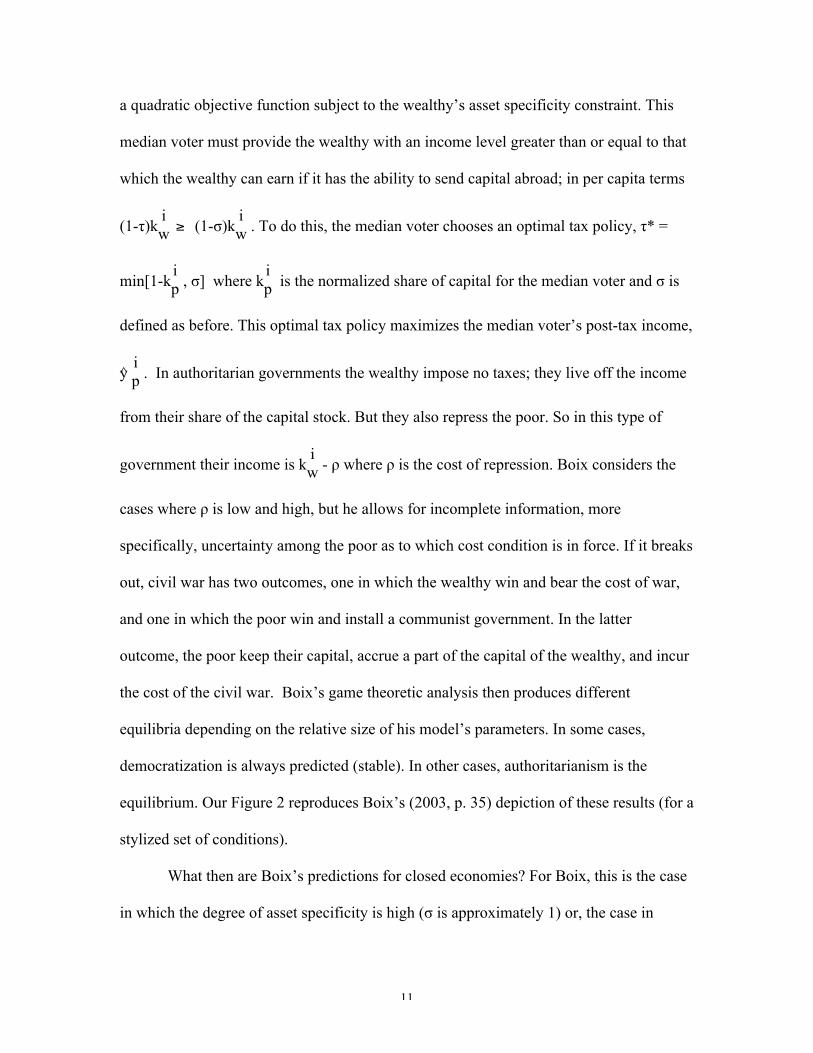
a quadratic objective function subject to the wealthy’s asset specificity constraint. This

median voter must provide the wealthy with an income level greater than or equal to that

which the wealthy can earn if it has the ability to send capital abroad; in per capita terms

(1-τ)kiw (1-σ)k

iw . To do this, the median voter chooses an optimal tax policy, τ* =

min[1-kip , σ] where k

ip is the normalized share of capital for the median voter and σ is

defined as before. This optimal tax policy maximizes the median voter’s post-tax income,

y ip . In authoritarian governments the wealthy impose no taxes; they live off the income

from their share of the capital stock. But they also repress the poor. So in this type of

government their income is kiw - ρ where ρ is the cost of repression. Boix considers the

cases where ρ is low and high, but he allows for incomplete information, more

specifically, uncertainty among the poor as to which cost condition is in force. If it breaks

out, civil war has two outcomes, one in which the wealthy win and bear the cost of war,

and one in which the poor win and install a communist government. In the latter

outcome, the poor keep their capital, accrue a part of the capital of the wealthy, and incur

the cost of the civil war. Boix’s game theoretic analysis then produces different

equilibria depending on the relative size of his model’s parameters. In some cases,

democratization is always predicted (stable). In other cases, authoritarianism is the

equilibrium. Our Figure 2 reproduces Boix’s (2003, p. 35) depiction of these results (for a

stylized set of conditions).

What then are Boix’s predictions for closed economies? For Boix, this is the case

in which the degree of asset specificity is high (σ is approximately 1) or, the case in

12

which there is no possibility of the wealthy earning income from abroad. If, in this case,

inequality is low, Boix contends the wealthy will always agree to democratize. The

optimal tax policy will not be constrained by σ, but the optimal tax rate for the median

voter, (1-kip ) will be relatively low because the gap in the income between the median

voter and the wealthy is low. The illustration in Appendix Figure A1 shows this for

income inequality in the range of 0-.2.

This prediction is different from that of AR, however. Recall that AR predict

authoritarianism for low levels of inequality in closed economies. For high levels of

inequality in the closed economy (σ near 1), Boix’s prediction is authoritarianism if not

civil war [northeast region of Figure 2). This prediction is the same as AR. Finally, for

intermediate levels of inequality in the closed economy (σ near 1), there is a cut point at

which it is rational for the wealthy to repress in order to preserve authoritarian

government. The location of this cut point and, by implication, the level of optimal

taxation for the median voter that provokes authoritarianism depends on the constellation

of the parameters in the model especially the cost of repression. To be more specific, at

intermediate levels of inequality, the key relationship is ( kiw -ρlow) > y

iw > (k

iw -ρhigh);

This condition determines whether, net of the (low) repression, the wealthy are better off

with authoritarianism than with democracy. So Boix’s prediction for the closed economy

(σ near 1) is a step change from democracy to authoritarianism as inequality increases

rather than a smooth transition (hump) from a low to high and then high to low

probability of democracy as inequality increases.

In sum, Boix’s proposition

13

Boix Proposition 1.

For closed economies (σ near 1), as inequality increases there is a step change in the prospects for democracy. Democracy is likely at low levels of societal inequality. But at an intermediate point that depends on a constellation of parameters, there is a switch to substantially decreased (no) prospects for democracy for this intermediate level of inequality and for all higher levels of inequality.13

The Economic Determinants of Democracy in Open Economies

How does economic globalization figure in these arguments? International

economic forces further enhance the prospects for democratization for both sets of

scholars. AR assume that in most autocratic countries labor is abundant and capital is

scarce. They also assume that trade produces factor price equalization. The result is an

increase in the returns to poor--an increase in the poor’s income--and a reduction in the

poor’s preferred tax rate. After trade, a relatively lower income loss to the rich relative to

the poor is sufficient to make democracy the preferred choice over repression (because

democracy means a higher post-tax income when the poor (median voter) chooses the

lower, post trade tax rate).

Capital mobility supposedly has some of the same effect as trade on the prospects

for democratization. Capital inflows occur in developing countries, because the return to

capital is higher domestically than internationally; eventually these rates of return are

assumed to equalize at which point capital inflows stop. The equalization (increase) in

wage rates occurs at the same time and, again, this lowers the preferred tax rate of the

poor, making democracy relatively more attractive than repression. This impact on wage

rates is sufficient to make democracy more likely. One reason is that, in their analysis of

13Because he emphasizes the conditions in which democracy is likely rather than the distinction between closed and open economies, Boix’s discussion (2003,pps. 32ff) is organized around the conditions in which democracy or authoritarianism are the equilibria of the game. We therefore reorganize his results here around the size of σ.

14

the inflow case, AR assume there are no local taxes on foreign capital and no taxation of

capital abroad.14

In regards to capital outflows, AR assume a global (post-tax) rate of return on

capital that is higher than the domestic (post-tax) return. They contend that, in

democracy, the poor are forced to equalize the two rates, or capital will flow out of the

country (reducing post-tax income). As with trade, this lowers the preferred tax rate for

the poor (median voter) to some p < τp. This, again, makes the payoff of democracy

relatively higher to the rich than it would be without capital outflows. In turn, repression

is less attractive. To be more specific, with capital outflow, repression has to be cheaper

(because there is less of an income loss) for it to be preferred by the rich. Thus,

democratization is encouraged by capital outflows.

AR’s analysis of the impact of economic openness on democratization produces a

clear causal expectation:

AR Proposition 2. In developing countries, both inward capital account liberalization and outward capital account liberalization lead to democratization though the mechanisms differ; inward liberalization leads to reductions in inequality, and outward liberalization limits redistributive taxation.

Again, in Boix’s model the key indicator of openness is asset specificity. This is a

parameter representing a reduction in the cost of moving capital away from its country of

14 AR also assume no cost to foreign capital from coups. They do not say if there is a cost to foreign capital from revolution. It appears this cost also ruled out by AR. This argument about capital inflows is for the developed country case. In the opening to the chapter on opening economies, AR point out that effects on wages and on capital are reversed in developed countries. In this case, wages fall and the returns to capital rise. But since these countries have “fully consolidated democracies” the implied, resulting “marginal increase in redistribution” will not provoke a coup. In other words, parameter values depend on the duration of democratic consolidation (see AR p. 323).

15

origin.15 The less “specific” the asset, the more mobile is capital. The link between

lower asset specificity (capital mobility) and democracy is straightforward, he argues:

….this book predicts that a decline in the extent to which capital can be either taxed or expropriated as result of its characteristics also fosters the emergence of a democratic regime. As the mobility of capital increases, tax rates necessarily decline since otherwise capital holders would have an incentive to transfer their assets abroad (2003, p. 12).

In terms of Boix’s model, recall that in democracy the optimal tax rate for the median

voter, τ*, is the minimum of (1-kip ) and σ. So, a low level of σ reduces the (poor) median

voter’s optimal tax rate. This means that taxation in democracy in an open economy has a

less redistributive impact on the income of the wealthy. Hence they are more prone to

accept democracy. [This is depicted in the illustration in the far left side of the Figure 2 .]

Boix mentions this as one of his principal results; democracy always occurs when asset

specificity is low (2003:32). But he makes only passing reference to how financial

liberalization is produces a decline in σ and therefore, all things being equal, enhances the

prospects for democracy (Ibid.p. 41) As regards trade, like AR, Boix contends that when

the poor are an abundant factor in world production, trade liberalization raises their

relative incomes therefore lowering the optimal tax rate and making democracy more

likely.16

Boix Proposition 2.

As economies become more open (σ approaches 0), democracy is increasingly likely.

15 Readers of the literatures in international business and foreign direct investment will note immediately that scholars in these fields see the international investment assets of globalized firms as being highly specialized and “specific,” far more so than investments of purely domestic firms. 16 In Chapter 4 of his book, Boix briefly argues that the skill distribution is the key factor mitigating the effects of trade liberalization. If the labor market is dominated by highly skilled individuals who benefit from trade, the prospects for democracy may be undermined. In this context he also mentions the salutatory effects of labor outflows on the prospects for democracy (by raising the relative income of the median voter and hence lowering the optimal tax rate). See 2003, pps. 142-143.

16

Critique

Financial Globalization and Capital Taxation.

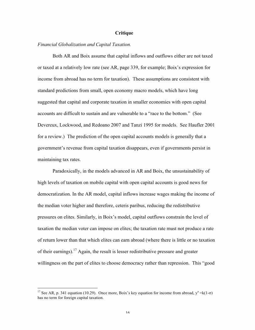
Both AR and Boix assume that capital inflows and outflows either are not taxed

or taxed at a relatively low rate (see AR, page 339, for example; Boix’s expression for

income from abroad has no term for taxation). These assumptions are consistent with

standard predictions from small, open economy macro models, which have long

suggested that capital and corporate taxation in smaller economies with open capital

accounts are difficult to sustain and are vulnerable to a “race to the bottom.” (See

Devereux, Lockwood, and Redoano 2007 and Tanzi 1995 for models. See Haufler 2001

for a review.) The prediction of the open capital accounts models is generally that a

government’s revenue from capital taxation disappears, even if governments persist in

maintaining tax rates.

Paradoxically, in the models advanced in AR and Boix, the unsustainability of

high levels of taxation on mobile capital with open capital accounts is good news for

democratization. In the AR model, capital inflows increase wages making the income of

the median voter higher and therefore, ceteris paribus, reducing the redistributive

pressures on elites. Similarly, in Boix’s model, capital outflows constrain the level of

taxation the median voter can impose on elites; the taxation rate must not produce a rate

of return lower than that which elites can earn abroad (where there is little or no taxation

of their earnings).17 Again, the result is lesser redistributive pressure and greater

willingness on the part of elites to choose democracy rather than repression. This “good

17 See AR, p. 341 equation (10.29). Once more, Boix’s key equation for income from abroad, ya =k(1-σ) has no term for foreign capital taxation.

17

news” is a reversal of sorts of earlier arguments made in political science that open

capital accounts diminish the prospects for democratization.

It is difficult, however, to think of an argument in international political economy

research that is more at odds with the observed behavior of governments. Consider

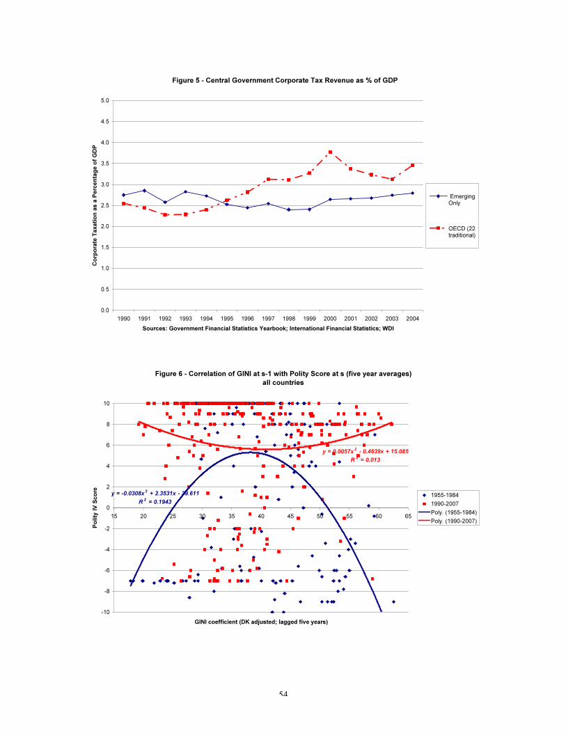
Figures 3, 4, and 5.18 Figures 3 and 4 report OECD corporate tax collections and rates for

1970 and 2005, both years of world business cycle expansion.19 For the average OECD

country, corporate tax revenues as a percentage of GDP have risen in the past 35 years

from 2.5% of GDP to 3.6%. The 35 years between 1970 and 2005 are a period of

financial globalization among OECD countries with no significant capital controls

remaining in 2005. Top corporate tax rates have fallen on average during the same

period (see Figure 4), but the tax base has been broadened through reductions in

incentives and other deductions, and base-broadening has contributed to the steep rise in

corporate tax collections.20 Emerging market corporate tax collections (Figure 5) in

recent years have not grown, in contrast to collections for OECD member countries, but

they have remained relatively stable.

Addressing the discrepancy between theory and evidence in a paper entitled

“Why is there no race to the bottom in capital taxation?,” Plümper, Troeger, and Winner

(2009) argue that fiscal rules and equity norms (measured by Gini coefficients) put

upward pressure on capital taxation, both rates and revenue. While “tax competition”

does cause some shifting of tax burdens to less mobile factors, fiscal rules and social 18 We use corporate capital taxation (revenue and rates) as our proxy for capital taxation. Data on corporate taxation is reliable, in contrast to data for the more general category, “capital” taxation. What constitutes “capital” income varies extensively cross-nationally in contrast to corporate income. 19 Because taxation is frequently counter-cyclical, controlling for stages of the business cycle is important in analysis over time. Both 1970 and 2005 were part of peak world business cycles with world growth averaging 5% both year. See IMF, World Economic Outlook, April 2007, p. 1. 20 See Devereux, Griffith, and Klemm 2002 for a review of the policy debate around cutting top tax rates while “tax-base broadening.” See also Swank and Steinmo 2002.

18

fairness norms are the determining factors. Plumper et al’s results confirm that countries

with open capital account do not converge on capital tax policies in general, and do not

“race to the bottom” in particular. Hays (2003) traces these differences in capital tax

policies to the workings of majoritarian versus consensual political institutions. The

Plumper et al. findings are consistent with the “system of constraints” argument and

evidence in Swank and Steinmo (2002), and the “tournament” model in Basinger and

Hallerberg (2004). Countries, while not free in these analyses to tax capital at

confiscatory rates, are able to capture substantial income from capital taxation under

conditions of capital account openness.

The implication is that the analyses in AR and Boix are seriously incomplete.

Governments are able to extract substantial revenue from owners of capital assets under

conditions of financial openness. Financial globalization does not necessarily eliminate

the tax burden on capital, and therefore the consequences of financial liberalization are

much more complex than AR and Boix argue. The foreign capital that flows into

countries is taxed therefore providing additional revenue for transfers to both the poor

and elite. How this additional revenue figures into the calculi of the median voter and

elite is not explained in either model. Similarly, elites contemplating capital flight must

take into account taxation abroad, which is extensive in advanced industrial economies.

This taxation necessarily lowers their potential income from abroad, and, in the case of

Boix’s model, means the impact of asset specificity is lessened. In turn, the optimal tax

for the median voter in the financially open economy may well be higher than Boix

suggests; the thresholds of inequality and asset specificity at which step changes from

democracy to authoritarianism occurs may be inaccurate. In particular, the possibility that

19

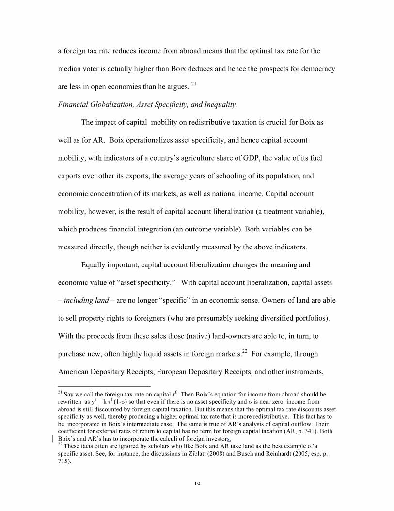
a foreign tax rate reduces income from abroad means that the optimal tax rate for the

median voter is actually higher than Boix deduces and hence the prospects for democracy

are less in open economies than he argues. 21

Financial Globalization, Asset Specificity, and Inequality.

The impact of capital mobility on redistributive taxation is crucial for Boix as

well as for AR. Boix operationalizes asset specificity, and hence capital account

mobility, with indicators of a country’s agriculture share of GDP, the value of its fuel

exports over other its exports, the average years of schooling of its population, and

economic concentration of its markets, as well as national income. Capital account

mobility, however, is the result of capital account liberalization (a treatment variable),

which produces financial integration (an outcome variable). Both variables can be

measured directly, though neither is evidently measured by the above indicators.

Equally important, capital account liberalization changes the meaning and

economic value of “asset specificity.” With capital account liberalization, capital assets

– including land – are no longer “specific” in an economic sense. Owners of land are able

to sell property rights to foreigners (who are presumably seeking diversified portfolios).

With the proceeds from these sales those (native) land-owners are able to, in turn, to

purchase new, often highly liquid assets in foreign markets.22 For example, through

American Depositary Receipts, European Depositary Receipts, and other instruments,

21 Say we call the foreign tax rate on capital τf.. Then Boix’s equation for income from abroad should be rewritten as ya = k τf (1-σ) so that even if there is no asset specificity and σ is near zero, income from abroad is still discounted by foreign capital taxation. But this means that the optimal tax rate discounts asset specificity as well, thereby producing a higher optimal tax rate that is more redistributive. This fact has to be incorporated in Boix’s intermediate case. The same is true of AR’s analysis of capital outflow. Their coefficient for external rates of return to capital has no term for foreign capital taxation (AR, p. 341). Both Boix’s and AR’s has to incorporate the calculi of foreign investors. 22 These facts often are ignored by scholars who like Boix and AR take land as the best example of a specific asset. See, for instance, the discussions in Ziblatt (2008) and Busch and Reinhardt (2005, esp. p. 715).

20

Argentine landowners now can sell their assets to overseas investors in American and

other equity markets, retain the proceeds from those sales and buy new equities. In

general, assets that were once treated as fixed or immobile (domestic asset owners

receiving little capital income abroad, or σ approaching 1) are now globally traded

(domestic asset owners receiving extensive capital income from abroad, or σ approaches

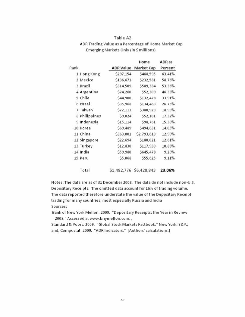
0). In fact, the public offerings in the American Depositary Receipt (ARD) markets by

industry – nearly 35% of the $175 Billion in offerings sold outside home countries have

been in ‘fixed’ or ‘immobile’ industries, such as mining and agriculture. Of the $6.5

trillion in market capitalization value for the top 15 emerging markets, nearly 25% of the

value of those markets traded in New York and not in the home market. These 15

emerging markets went from substantially closed in the early 1980s to substantially

financial open in the early 1990s. See Figure 8 (see also the Tables A.2 and A.3 in our

Appendix).. In addition to these 15 leading markets, international investors are buying

and leasing ‘immobile’ assets, such as large tracts of land in Africa, Central Europe, and

other parts of the world. The Economist calls this “Outsourcing’s Third Wave” (May 23,

2009: 61-62). Even labor is not quite so “specific” as laborers can sell “labor” to foreign

investors, and these workers can invest the returns of their labor in overseas markets.

Modern portfolio theory sheds light on how liberalizing both capital account

inflows and outflows helps domestic and foreign investors create better diversified

portfolios. A central problem for international investors has been to diversify risk by

investing in assets that do not commove with international markets. Paradoxically, when

a country with ‘immobile’ assets liberalizes inward capital account transactions, specific

assets (or those that have idiosyncratic risk that are uncorrelated with returns in global

21

capital markets) become highly valuable to foreign investors as components of a

diversified portfolio. With liberalization of capital account outflows, the domestic

investor is able to avoid insuring that that his or her assets are not too “specific” (or, more

correctly, not too idiosyncratic in risk) through international diversification.

The key recommendations of modern portfolio theory - international

diversification is good for domestic investors and domestic investment is good for

international investors – has a long lineage of work. Lowenfeld (1909) demonstrated that

international equity market correlations are lower than industry correlations within one

country, a finding widely replicated since. Consequently, domestic investors should be

able to improve the risk/return profile of their portfolio significantly if they move assets

out of “specific” classes of investments, and partly into foreign equities and assets

(Grubel (1968), Levy and Sarnat (1970)). In these ways, capital account liberalization

has been a core, if not the core, contributing factor to asset market integration (Quinn and

Voth 2008).

Hence, we expect that, following capital account liberalization, domestic capital

owner will accrue large earnings through asset sales (leases) to foreigners. These earnings

will increase – not decrease – income inequality. Moreover, their ability to sell their

assets abroad (to foreigners) will reduce asset specificity even further. Whether foreign

capital in a country is more (as) productive as native capital thereby increasing the wages

of native workers—remains to be seen. Neither AR nor Boix analyze this possibility.23

Beyond this, there is the question of if, under financial liberalization, the cost of

23 AR’s (Chapter 10) analysis of capital inflow assumes that some new, externally supplied capital K’ simply is added to native capital K increasing productivity, wages, and hence reducing inequality. AR don’t address the possibility of foreign capital substituting for native capital. Boix does not have an economy in his model so he is unable to analyze this possibility.

22

repression necessarily falls more heavily on physical capital than land (AR, chapter 9)

and, now, for these reasons some of this cost also falls on foreign capital. The latter

possibility also is ignored by AR (Ibid., p. 339).

In addition, empirical studies offer some evidence that financial globalization will

lead to increasing income inequality. Financial globalization was found to be a robust

correlate of rising income inequality in a cross-section of countries examined in Quinn

1997. A recent paper by Jaumotte, Lall, and Papgeorgiou (2008) uses panel OLS

methods to disentangle the effects on income inequality of technological innovation,

trade, and financial globalization. They find that, while trade does have the effect of

reducing income inequality, inward FDI flows have increased not decreased income

inequality (cf. AR, Chapter 10, Section 5.1). A study in 2008 by the International Labor

Organization (ILO) also uses OLS panel methods to document the correlation between

rising income inequality and stock of FDI as a percentage of GDP (ILO 2008). [See also

Figini and Görg (2006), which show initial rises in wage inequality from inward FDI.]

In these ways, financial globalization has much more complex effects on

democratization than AR and Boix contend. In the short term, asset sales increase, rather

than decrease, inequality, thereby hurting democratic prospects. On the other hand, the

increasing ability of native elites to sell land and other assets limits the ability of the poor

to tax the elites and this should lessen elite opposition to democratization.

Tests of Economic Theories of Democratization

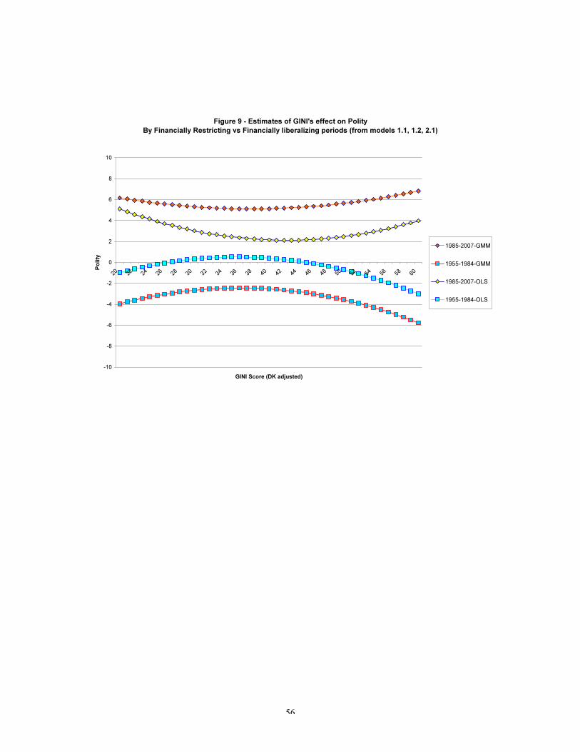
How well do the AR and Boix propositions match data for the postwar era? As a

simple experiment, we plot the lagged values of a country’s five year average GINI

coefficient and the five year average value of its Polity IV score: e.g., GINI 1955-59

23

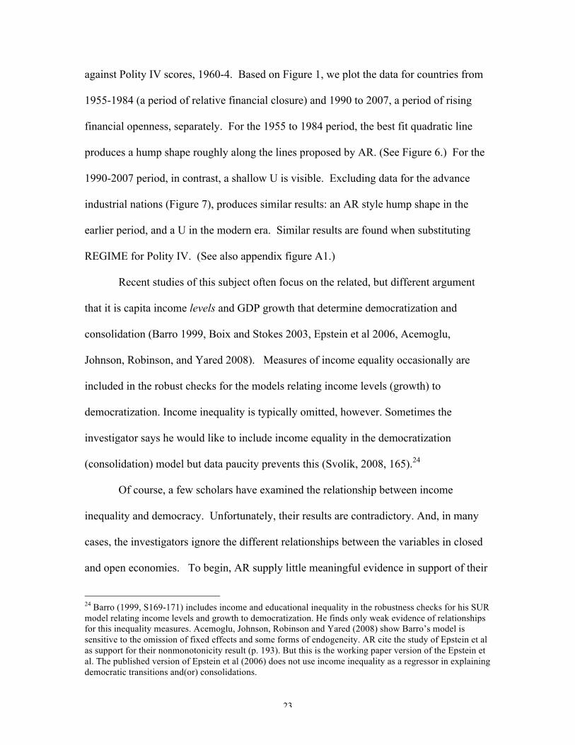
against Polity IV scores, 1960-4. Based on Figure 1, we plot the data for countries from

1955-1984 (a period of relative financial closure) and 1990 to 2007, a period of rising

financial openness, separately. For the 1955 to 1984 period, the best fit quadratic line

produces a hump shape roughly along the lines proposed by AR. (See Figure 6.) For the

1990-2007 period, in contrast, a shallow U is visible. Excluding data for the advance

industrial nations (Figure 7), produces similar results: an AR style hump shape in the

earlier period, and a U in the modern era. Similar results are found when substituting

REGIME for Polity IV. (See also appendix figure A1.)

Recent studies of this subject often focus on the related, but different argument

that it is capita income levels and GDP growth that determine democratization and

consolidation (Barro 1999, Boix and Stokes 2003, Epstein et al 2006, Acemoglu,

Johnson, Robinson, and Yared 2008). Measures of income equality occasionally are

included in the robust checks for the models relating income levels (growth) to

democratization. Income inequality is typically omitted, however. Sometimes the

investigator says he would like to include income equality in the democratization

(consolidation) model but data paucity prevents this (Svolik, 2008, 165).24

Of course, a few scholars have examined the relationship between income

inequality and democracy. Unfortunately, their results are contradictory. And, in many

cases, the investigators ignore the different relationships between the variables in closed

and open economies. To begin, AR supply little meaningful evidence in support of their

24 Barro (1999, S169-171) includes income and educational inequality in the robustness checks for his SUR model relating income levels and growth to democratization. He finds only weak evidence of relationships for this inequality measures. Acemoglu, Johnson, Robinson and Yared (2008) show Barro’s model is sensitive to the omission of fixed effects and some forms of endogeneity. AR cite the study of Epstein et al as support for their nonmonotonicity result (p. 193). But this is the working paper version of the Epstein et al. The published version of Epstein et al (2006) does not use income inequality as a regressor in explaining democratic transitions and(or) consolidations.

24

main argument that there is a hump-shaped relationship between income inequality and

democratization. AR offer a few scatterplots in support of the idea that income inequality

and democracy are correlated. These scatterplots, however, actually show a curiously

monotonic relationship (even though their central thesis is that the relationship is

nonmontonic).25 In fact, the relationship in AR’s main scatterplot looks more like that

predicted by Boix under conditions of high asset specificity (2003; see Figure A.2 in our

appendix). At no other place in their book do AR produce any statistical analysis in

support of their argument. In fact, in their analysis of the impact of international

economic forces on inequality and democracy, they admit that the evidence is “unsettled”

or “equivocal” (2006, 344-5, 347).

Boix, provides a rigorous test of his theory. Using five year Gini measures of

inequality from Denniger and Squires, the measures of asset specificity listed above,

Przeworksi et al’s classification of democracies, and Amemiya’s dynamic probit model,

he analyzed autocratic to democratic transitions from 1850-1980. Boix reported support

for his claim that there is an inverse relationship between inequality and democratization.

His result was robust to the omission of Soviet cases and some specification changes

A more recent test of AR and Boix’s claims is Houle (2009). Houle also uses a

dynamic probit model to predict transitions in the Przeworski et al’s measure of regime.

The data of Ortega and Rodriquez are used by Houle to measure inequality. His analysis

spans the period 1950-2002. Houle’s main finding is that inequality only affects the

25Later, in Chapter 6, AR report data on a single downturn in inequality in Korea-Taiwan and of a relatively flat trend in income inequality in Singapore (Figure 6.3, p. 192) as evidence of the nonmonotonic relationship. Needless to say, these data do not support the strong claim they make about nonmonotonicity. Below, we review the logic behind the thesis that income inequality of intermediate levels is only likely to produce democracy (2006, p. 37, 189-193).

25

consolidation process, not democratization; if there is any relationship between inequality

and democracy it is U not hump-shaped (Houle, 2009: 610, 615).

Several methodological problems plague these tests. First, Houle’s analysis does

not capture the essence of Boix’s argument. As explained above, Boix’s theory is based

on the conjuncture of income inequality and asset specificity (cf. Figure 2). Houle does

not include any variables (controls) for, let alone interactions with asset specificity.

Second, like Boix’s original test, Houle does not provide for variations in economic

openness. He includes a variable for oil exports in his model but only to test arguments

about resource determinants of democracy. The inclusion of time, e.g., decade dummies,

as proxies for financial and other kinds of openness obviously is problematic. Our review

of the open case implies that Houle’s, and even Boix’s, models are plagued by omitted

variable bias.26

Last, and probably most important, is the problem of endogeneity. Consider the

following schematic representation of the argument in AR’s tenth chapter linking

financial openness to democratization:

1) Inward Financial openness → factor price equalization → greater income

equality → democracy is likely to result in less redistribution and repression is relatively

less attractive in relation to democracy → greater probability of transition to democracy

(and of democratic consolidation).;

and

26 Houle (2009) includes both trade and land in his multiple imputation model but, for some reason, not in his explanatory models. Ansell and Samuels (2009) also miss the importance of asset specificity in Boix’s argument. They too make no provision for the effects of economic openness on link between income inequality, asset specificity, and democratization.

26

2) Outward financial openness → greater incentives for capital flight for elites in

the presence of high tax policies imposed by democracy → reduction in median voter’s

preferred tax rate to somewhere between “safe haven” and global average tax rate →

democracy is likely to result in less redistribution, and repression is relatively less

attractive in relation to democracy → greater probability of transition to democracy (and

of democratic consolidation).

This causal chain is a recursion and therefore relatively easy to estimate. But, if

the causal arrows point in both directions, models like those of Houle and others that treat

inequality and other covariates as exogenous will be plagued by endogeneity bias. And

there are many places in AR’s analysis that suggest endogeneity is present. One is their

analysis of the impact of concessionary taxation in autocracy; concessionary taxation

may affect income inequality.27 Statistical tests therefore not only must “control” for the

variables left out of AR’s analysis but also estimation must take endogeneity into

account. Unfortunately, AR give us little guidance how best to accomplish these things.28

In Boix’s case, the core argument is that it is actor expectations about how elites and

“masses” pursue or resist future democratization in light of their preferences regarding

current and future distributions of income that influence the likelihood of a country’s

27 AR treat the level of income inequality in autocracy as exogenous, fixed parameter. Yet one of their main insights is that the rich, under certain conditions, can (promise to) redistribute some income to stave off revolution; this rate is expressed in equation (2) in the text. How this concessionary taxation affects the level of income inequality is not clear. In addition, AR go back and forth—sometimes even in the same passage (e.g., p. 189) between talking about the promise to redistribute income via concessionary taxation and the actual redistribution of concessionary taxes. They also do this in their dynamic analysis (pps. 198-199). Once more, how concessionary taxation and redistribution could leave θ unaffected is not explained. Another likely form of endogeneity is the relationship between capital outflows and the size of the capital stock. The loss of capital in this case may have the same impact as the loss of capital due to revolution or coups. 28 Boix acknowledges that the democracy and inequality variables are endogenous, especially in a cross-sectional research design (2003, 74). But, Boix says “even if inequality is an endogenous variable to political regime, it is determined previously to the political game we are playing.” If, as Chong 2004 and others note, independent and dependent variables exhibit persistence over time, an instrumenting procedure is advisable.

27

democratization. Therefore, expectations of about future democracy potentially influence

current distribution of resources; and, expectations about future democracy influences

expectations about future income distribution, all of which in turn is correlated with

current distribution.

Finally, note that many papers explicitly reverse the dependent and independent

variables in the AR and Boix investigations, and instead model the effect of democracy

and autocracy on income inequality (Reuveny and Li 2003, for instance). Some recent

papers model the relationships endogenously; see, e.g., Chong 2004 (especially 193, 203)

in which a GMM_System set-up is used to explore the effects of democracy on changes

in inequality. We content that because of the possibility of endogeneity, econometric

analysis must employ instrumental variables methods.

Our Argument

We agree that the relationship among financial globalization, rising inequality,

and democratic prospects is non-linear, as AR suggest. But we contend that the

nonlinearity reverses in the presence of financial globalization. In relatively equitable

societies, financial globalization increases inequality since it affords elites more

opportunities to increase their wealth through asset sales, but gains from taxation to the

poor and the losses to the rich, given by the constrained global rate, are modest. Hence

democratization is likely in financially open economies with low levels of inequality. In

conditions of intermediate inequality, however, with financial globalization and asset

sales comes a further increase in inequality, which is likely to hurt democratic prospects

as the holders of rising incomes risk being taxed by the poor at the global tax rates, which

are far from zero. As inequality rises to high to even higher levels, however, the poor are

28

faced with a global tax rate constraint and the possibility of large number of asset sales,

limiting the scope of redistribution. Moreover, once income inequality rises to high

levels, prudent wealthy residents are likely follow the advice of modern portfolio theory,

which is to diversify internationally. The wealthy have little to gain from resisting

democratization. Therefore the prospects for democratization are bright in financially

open economies with high inequality. Given financial globalization, very low and very

high levels of inequality, therefore are associated with democratization. Again, at

intermediate levels of inequality, the ability of elites (asset holders) to diversify are more

limited, making capital exports more difficult. Capital tax rates are biting at intermediate

levels of inequality. Hence this is the case where the prospects for democratization are

least favorable in the financially open case.

Schematically, we differ most from AR in terms of the influence of inward

liberalization:

1) Inward Financial openness → factor price shifts, asset price auctions and

bubbles from international investors seeking ‘asset specificity’ → greater income

INequality as holders of tangible assets gain windfalls → democracy is more

likely to result in more redistribution; and repression is relatively more attractive

in relation to democracy → lower probability of transition to democracy (and of

democratic consolidation); and

2) Outward financial openness → international portfolio diversification by

domestic elites → reduced internal income inequality → reduction in median

voter’s preferred tax rate to somewhere between “safe haven” and global average

tax rate → democracy is likely to result in less redistribution, and repression is

29

relatively less attractive in relation to democracy → greater probability of

transition to democracy (and of democratic consolidation).

We therefore propose that – with greater financial liberalization – comes a U.

Relatively equitable autocracies have few incentives to resist democratization, as Boix

argues, under conditions of financial openness. With increased but moderate levels of

inequality, the wealthy have an incentive to resist democracy as globalization produces

windfall returns. Once inequality rises to high levels, the wealthy in open societies have

few incentives to resist democracy as the democratic tax rate is constrained to be at or

near the global average and opportunities to diversify through international asset sales are

lucrative and many.

Summary and Hypothesis. AR argue that financial globalization should lead to

democratization, both because of the decreasing inequality from factor price equilibration

in emerging markets, and from the diminished ability of the state to tax and redistribute

capital income. Boix sees decreasing inequality directly, decreasing inequality from

financial globalization indirectly, and financial globalization per se all reinforcing

democratization. The relationship between financial globalization and democratization is

linear and positive for both Boix and AR.

We contend, in contrast, that financial globalization, especially inward

liberalization, leads to rising – not decreasing – inequality. We further propose that

outward liberalization, which offers elites the opportunity to sell their land as well as

other assets abroad, while constraining of some government policies, still allows for

significant redistribution of wealth through the tax system .These relationships produce a

U-shape relationship among financial globalization, inequality, and democracy.

30

The next sections describe the data used and put forth such a design. We then

conduct a test of these propositions.

A Test of Our Theory

Data and Measures

Data choices significantly influence many scholarly studies. We outline here

some of the choices investigators face in estimating models using measures of

democracy, inequality, and financial globalization. We then assess the consequences of

these choices. Where feasible we use multiple indicators of key variables.

Democracy. Our core dependent variable in this investigation is democracy, which we

measure by using both Polity IV and Regime.29 These democracy measures are standards

in political economy. We estimate models using the two variables to demonstrate

robustness of our results. In using the 21 point Polity measure, we allow for minor as well

as major changes in democratic institutions to be modeled. In using the 0,1 Regime

variable, we focus on large changes in political institutions. (Note that in a five year

panel, the dichotomous Regime variable is transformed into an interval level variable

taking values between 0 and 1, and which is continuous and normally distributed).

Regime is rescaled so that large values indicate greater levels of democracy or of civil

liberties. As an additional robustness check, we estimate models using Freedom House

data, though note that the limited coverage in Freedom House (1972 onward) limits our

ability to test propositions about financial closure.

29 Polity IV is from Marshall, Jaggers and Gurr 2007 (updated at www.bsos.umd.edu/cidcm/polity). Regime is from Przeworski et al. 2000 (upates available from Cheibub and Ghandi 2004, as cited by http://www.nsd.uib.no/macrodataguide/set.html?id=1&sub=1.

31

We show below that the choice of the democracy indicator is not per se a crucial

choice in the investigation. Regime, however, has fewer observations than Polity IV, and

the end of the respective series coincides with important changes in history. But, regime

ends in 2000, and misses recent events. Polity IV covers the period between 1945 and

2007, and therefore contains more variance.

Inequality. In contrast to the democracy indicators, which are broadly comparable across

space and time, the cross-national inequality indicators are plagued with measurement

difficulties. We use as our measure of inequality Gini coefficients30 from three standards

sources: Deininger and Squires 1996 (D&S); Milanovic 2005, and United Nations

University-World Institute for Development Economics Research’s World Income

Inequality Database (WIID) 2008. The D&S and WIID data, however, contain

information from diverse sources using diverse methods on diverse populations. These

data need to be adjusted before using in cross-national, time-series analyses.31 The

Milanovic/World Bank survey data are comparable across time and space, but are limited

in time to at most three observations per country.

Dollar and Kraay 2002 (DK) offer a transforming metrics that allow for the GINI

indicators to be turned into measures useful for comparative research. 32 We use DK’s

transformation algorithm to adjust the 2008 WIID data.

30 Gini coefficients are a way of measure a nation’s income inequality. They are scaled between 0-100. Gini coefficients measure the dispersion of income, with high values indicating higher inequality. 31 The main differences are whether surveys measure income or expenditure, households or individuals, and are net of taxes and transfers or are gross income. We use GINI indicators that are a) national in origin, b) are rated as having a WIID quality of at least “3,” and c) where possible, consistent by methodology within country. 32 Dollar and Kraay 2002 (Table 2) use a regression on GINI using dummy variables for gross income and expenditure (consumption), plus regional dummies. They then subtracted the coefficient estimates of the gross income and expenditure dummies from the GINI coefficient. Identical results are given by extracting the residuals of the regression, and adding them to the intercept. Dollar and Kraay did not use a dummy for household vs. person as they do not find a statistically significant effect (Email correspondence, A. Kraay

32

The Galbraith and Kum 2005 inequality indicator, EHII, uses United Nations

Industrial Organization (UNIDO) wage data with a Theil T’s statistic to generate over

3,000 country year observations of GINI. An advantage of the Galbraith-Kum approach

is that a fuller data set using wage data is estimated. A disadvantage is that their data end

in 1999, whereas the new WIID data extend to 2006. The correlation between EHII and

the other GINI indicator is not high: ~.6. We show below that the results of the

investigation will sometimes differ, depending on which of these GINI indicators are

used.

An alternative measure of inequality is used by Houle 2009. Houle uses the

UNIDO data without the Galbraith-Kum adjustments, and describes these data as “capital

share” data, following Rodriguez and Ortega 2006. Rodriguez and Ortega 2006 do not,

however, treat the “capital share” as cross-nationally valid indicators of inequality.

Rodriguez and Ortega demonstrate that per capita income and national ‘capital

share’ from UNIDO exhibit a strongly negative, highly statistically significant,

relationship in a variety of specifications. (See their Figure 1 (2006, 4) plus their results

section) In contrast, controlling for country effects, the WIID indicators with a DK

adjustment have no statistically significant relationship with per capita income.

It is initially extremely counter-intuitive that capital poor countries would exhibit

high capital shares relative to capital rich countries. One possible explanation for this

anomaly is discussed in Rodriguez and Ortega 2006, which is measurement error and

and D. Quinn, 21 July 2008; phone conversation, 17 July 2008.) We replicate nearly exactly Dollar and Kraay’s results for Table 2 on their sample. In the WIID 2008 updated sample, however, we find that the coefficient estimate for household is now statistically significant, and that the regional dummy effects in Dollar and Kraay are now very different from prior findings. A simple model regressing GINI with dummies for all three types of surveys is what we use. We also estimate a model without the household dummy. The coefficient estimate for expenditure surveys remains consistent with the early Dollar Kraay result, but the coefficient on the gross income dummy is now twice the size as before. We use both results.

33

national differences in reporting. Since capital share (CS) is taken as CS =[1-Wages and

Salaries], and since it is computed from surveys of larger incorporated firms, countries

with large informal sectors or many smaller business will, through data omission on wage

data, have larger capital shares (since the wages paid in the informal sector and in small

businesses will be credited to the capital share). Many advanced economies also report

fringe benefits and other forms of compensation as wages, which further decreases their

capital share. A second possibility that Rodriguez and Ortega consider is that poorer

countries have stronger agrarian sectors, which are not considered in the industrial

surveys. A third possibility is that emerging market countries, while having fewer

incorporated firms and larger agrarian sectors, also have firms that exhibit lower labor

productivity, which translates into lower wages (and higher capital shares). A fourth

possibility, and highly germane to the research question, is that more open societies,

which tend to be richer, do a better job of collecting survey data from respondent firms.

Whatever the advantages of the capital share measure from UNIDO, the data

appear to be highly influenced by collection and reporting methods, which are in turn

correlated with several of our key independent and dependent variables. The WIID data,

in contrast, do not exhibit a correlation with indicators of development. (EHII, which is

based on UNIDO, does have a modestly negative statistically significant correlation with

income, which must be counted as a disadvantage in this investigation.)

Financial Globalization. We operationalize international financial regulation as two

indicators of change in international financial openness or closure, which are described in

Quinn (1997) and Quinn and Toyoda (2007; 2008). CAPITAL and

FINANCIAL_CURRENT (FIN_CURRENT hereafter) are the main components of

34

openness created from the text published in the annual AREAER volume that reports on

the laws used to govern international financial transactions. These indicators take a

different approach in creating an index for a government’s policy stance toward capital

account liberalization and financial current account liberalization by offering a measure

not only for the existence (absence) of restrictions, but also for the severity or magnitude

of those restrictions. Data for up to 122 countries through 2007 are available. CAPITAL

is scored 0-4, in half integer units, with 4 representing an economy fully open to capital

flows. This measure is transformed into a 0 to 100 scale by calculating

100*(CAPITAL/4). CAPITAL distinguishes between restrictions on residents and non-

residents, which correspond to restrictions on capital outflows and inflows, respectively.

(See IMF (1993), pp. 80-1, for a discussion).

To measure a country’s integration into global financial markets, scholars often

turn to non-index, de facto or “blended” measurements. Reuveny and Li 2003, for

example, used FDI inflows and Portfolio inflows as indicators of financial globalization

in their study.

In this investigation, however, we cannot use FDI and portfolio indicators as

measures of financial globalization. Our analysis spans 1955 to 2007, a time period in

which four different “investment regimes” prevailed, rendering the FDI and Portfolio

measures not comparable across investment regime. To be specific, the 1993 IMF

Balance of Payments Manual (BoPM), 5th edition, revised the definition of FDI as

constituting the purchase by non-residents of 10% or more of the ordinary shares (or

voting equity stake) of a company. The 4th edition (IMF (1977), 137) gave a range of 10

35

to 25% to distinguish FDI from portfolio investment. The 3rd edition (IMF (1961), 120)

gave a range of 25 to 75%, depending on the circumstances.

The data reported for FDI and portfolio flows are not adjusted back in time, with

the result that some of the increases in FDI flows in the 1990s in particular derive from

changes in threshold definition for FDI: 10-25% of an investment stake vs. 10% after

1993. Moreover, countries used and continue to use inconsistent definitions, albeit with

IMF permission. See IMF (1996) and IMF (1993, 87).33 Because of the inconsistencies

in FDI and portfolio data across time, we use the de jure measures of financial

globalization.

Models and methods. In this investigation, we are interested in exploring the

separate and joint effects of financial globalization and income inequality on

democratization. Pooled, cross-section, time-series (PCSTS) models are useful in

evaluating the question of why, over time, some countries become more democratic while

others do not. That is, the variation in the dependent variables comes from both the

dynamic and cross-sectional factors. Some pooling of data is necessary to address the

questions.

Because AR (2006) offer little guidance regarding the appropriate design for their

propositions, we start with models of five year averages of democratization proposed and

estimated in their related work, Acemoglu, Johnson, Robinson, and Yared 2008, hereafter

AJRY. The AJRY model is a country and time fixed effect model with an indicator of

Democracy in levels as a dependent variable estimated with a lagged endogenous

33 The discussion group for the 6th edition of the BoPM, scheduled for release in 2008, has proposed 20% as the new threshold for distinguishing FDI flows from Portfolio flows.

36

variable on the right-hand side. In their specification, AJRY add one key variable, log of

income, lagged once.

We find, as AJRY do, persistent serial correlation in their simple model using five

year averages. We overcome the serial correlation by amending their model with an

additional lag of the level of the dependent variable. (See also Barro 1999). By

including lagged levels of the dependent variable, we no longer include country fixed

effects in the model (as the inclusion of fixed effects induces serial correlation in these

OLS models, presumably because of the correlation between the fixed effects and the

lagged dependent variables). These OLS specifications are five-year non-overlapping

models, with the units denoted by i=1,2,...,x and the index s representing five-year

intervals, starting at 1955-59 and continuing onward. This means, e.g., that

Democracyi,s for the s=1985-1989 period is analyzed using data from the s-1=1980-84

period. This is in contrast to AJRY, who use the initial year’s value to represent the data

for a five year period.34

We use this simple OLS AJRY model to explore the potentially nonlinear

relationship derived in AR between inequality and subsequent democratization,

employing various indicators of inequality. A hump shaped relationship, as derived by

AR in their Corollary 6.1, would imply that intermediate levels of inequality facilitate

democratization. This relationship would appear as a statistically significant positive

coefficient on the level of Gini and a statistically significant negative coefficient on Gini

squared. A “U”-shaped relationship between the two variables would have the opposite

34 The data for Polity are up through 2007. The data for 2005, 2006, and 2007 are averaged in a period, and examined using data for the right hand-side variables for 2000-04. The Regime series data are through 2002, and the 2000, 2001, and 2002 data are average into a single period, and examined using data on the right hand side from 1995-1999.

37

signs on the respective coefficients. This U shape would imply, contrary to AR’s

Corollary 6.1, that low and high levels of income inequality facilitate democratization.

Again, we theorize that the coefficient estimates will vary such that, in eras of

financial closure, inequality will have a non-linear relationship as proposed by AR – a

hump. In eras of financial openness, in contrast, inequality’s non-linear relationship will

invert – a U shape will appear. To test our hypotheses, we divide the data into two

periods based upon Figure 1, 1955 to 1984, and 1985 to the present. 35

OLS estimations, while useful in exploring the structure of the relationships, are

potentially plagued by several methodological problems including 1) hard-to-observe

persistence in explanatory variables that is correlated with the error term and 2) possible

endogeneity. As explained above, we test for serial correlation, and find that, as did

AJRY, models with one lag of the dependent variable are plagued with extensive serial

correlation. We find, however, our democratization models, two or three lags of the

lagged endogenous variable invariably eliminate evidence of serial correlation.

The endogeneity problem for the relationships between democracy and economic

inequality is unquestionably serious, given that scholars treat both variables as dependent

and independent. Some scholars focus on the contemporaneous effects of democracy on

inequality (e.g., Reuveny and Li 2003), while others focus on the effects of inequality on

democracy (e.g., Acemoglu and Robinson 2006). The relationship between financial

globalization and democracy is also potentially endogenous. For example, Quinn and

Toyoda 2007 analyze democracy’s influence on financial globalization whereas Guiliano,

Mishra, Scalise, and Spilimbergo 2008 examine the reverse relationship. Eichengreen

35 Financial closure, not openness, spread world-wide until the early 1980s, with the 1980-4 period representing the ‘low’ point of financial globalization in our models.

38

and Leblang find a mutually reinforcing relationship between democratization and

financial globalization in an instrument variable (IV) setup. (See also Giavazzi and

Tabellini 2006; Milner and Murkerjee 2009.) Five year lagged averages in variables

attenuate the possible endogeneity bias, but they do not eliminate it.

To further address the endogeneity issues, we use GMM-system estimations,

which are a form of IV regression.36 The GMM_System method is due to Blundell and

Bond 1998; it is the same estimator used by Eichengreen and Leblang 2003, Mukherjee

and Milner 2009, and Quinn and Toyoda 2007, 2008, among others.

The validity of the instruments is assessed through the Sargan test of over-

identifying restrictions.37 The null hypothesis is that the instruments are uncorrelated

with the error term, and a rejection of the null hypothesis at conventional levels of

statistical significance means that instruments are not valid: the number in brackets is the

p-value of the test. For example, [1.000] equals a p-value of one, and indicates that the

instruments are valid.

Our design includes an additional transformation of the right-hand side variables.

The GINI estimates, the democracy variables, and other right-hand side variables exhibit

persistence over time, a persistence that is exaggerated by five year averaging. The same

is true of the lags of the endogenous variables we use as instruments. The persistence in

these variables could make them correlated with the error term. This would produce

biased estimates. We therefore difference these variables. Finally, note that in GMM

estimation, the absence of serial correlation in the main model is indicated by is indicated

36 All estimations are done using PCGive 12. 37 To be more specific, we use the two-step Sargan test, as recommended in Doornik and Hendry 2001, 69.

39

by negative, statistically significant first order AB m1 test, combined with no statistical

significance on the AB m2 test. (See Doornik and Hendry 2001, 69.)

The AJRY model, while the starting point for our investigation, is underspecified

regarding other determinants of democracy. We add to the base model for democracy

regressors representing domestic political and economic variables, most of which are

standard in the literature: growth in PPP adjusted per capita income, log of levels of

investment (as a share of GDP), and log of levels of trade openness (imports + exports as

a percentage of gross domestic product). (See Gassebner, Lamla, and Vreeland 2007 for

a review of some of the standard regressors in the literature. See also Milner and

Muhkerjee 2009.) We add to this model an indicator of change in global oil prices.

Recent scholarship stresses the importance of investigating and controlling for

unobserved cross-sectional or spatial correlation in time-series panel studies. (See

Franzese and Hays 2007.) Of particular concern in this investigation is whether the

changes in democratic processes for a given country are fully independent of the

processes at work regionally and(or) globally. Gleditsch and Ward (2006) find that a

country’s democratic processes are influenced by regional forces, as measured by

regional averages for democracy. To assess the influence of the behavior of regional

neighbors, we compute the regional average democracy for a given country (removing

the value for that country).38

With the differencing transformation, additional conditioning information

(controls) and allowance for endogeneity, the GMM-system model (1) is:

38 We use the World Bank’s regional definitions.

40

ΔDemocracyi,s = ß0 + ß1(ΔDemocracyi,s-1) + ß2(ΔDemocracyi,s-2 ) + ß3(ΔGINIi,s-1) +

ß4(ΔGINIsquarei,s-1) + ß5(ΔEconomic Growthi,s-1) + ß6(ΔIncomei,s-1 )

+ß7(ΔInvestmenti,s-1) + ß8(ΔTrade Opennessi,s-1) + ß9(ΔWorld Oil Pricesj,s-1) +

ß10(ΔRegional Democracy)j,s-1 + εi,s

i=1,2,...,84. (1)

The instruments for the endogenous variables in (1) are the third lags of the levels

of the endogenous variables, and the second lag of the differences of the endogenous

variables, except in the case of the democracy variables, where the fourth and third lags

(respectively) are used.39 Change in oil prices is treated as exogenous variables. Note

that this model includes the variables we need to test the main propositions in the AR’s

argument: GINI indicators (described above), and the squared GINI indicator terms. In

GMM system models, fixed effects can enter can enter the model (if the unit effects are

uncorrelated with the error term and with the instruments for the lagged endogenous

variable). We report the results of (1) with both fixed and random effects models. We

elsewhere test for fixed-effect, and estimate fixed effects models where appropriate.40

To test properly the second parts of AR’s and Boix’s arguments - the claims about

the impact of financial integration on inequality - we need to estimate models of income

inequality. As explained above, AR’s argument is that financial integration’s positive

influence on democracy works, at least in part, through changes in income inequality. 39 The model settings in PCGive 11 for the GMM system estimation include 1-step estimates with robust standard errors, the transformation set to ‘differences,’ and specification tests for two lags of serial correlation. 40 We estimate a Wald test version of the Hausman test. The classic Hausman test is whether the coefficient estimates from a random effects model are unaffected by the omission of unit effects; the null hypothesis is that the beta of fixed effects model equal the betas of random effects models. This will be true only if the fixed effects are jointly zero. We directly test whether the unit effects are zero with a Wald test.

41

AR further argue that Capital_In and Capital_Out have subtly different effects on

inequality, the rich, and therefore on the transition to democracy. (See especially pp.

338-340 on “Capital-in and Democracy,” and pp. 340-342 on “Capital-out and

Democracy.”)

Modeling inequality, however, requires adding additional information to the

inequality base model. As Tanzi (1998, 4) noted, “inequality is generally determined by

the interplay of various factors ….[of which] the main systemic factors are social norms

or institutions [and] broad economic changes….” We operationalize social norms in

terms of global anticapitalist sentiment, as in Quinn and Toyoda 2007.41 To represent

economic changes, we enter indicators of per capita income, investment, changes in

global oil prices, and population growth. We follow Reuveny and Li (2003) and add

trade openness to the model. We test for the “Kuznets effect” by adding income squared

as a regressor (Kuznets 1955). Because we find that the coefficient estimates of the

income squared indicator are always smaller than the corresponding standard errors, we

omit the term from the reported results. The capital account variables are central to the

analysis as AR suggest that easing both inward and outward capital restrictions will

influence inequality’s dynamics. Capital inflows should raise incomes of lower wage

workers in capital scare economies, and the threat of capital outflows should limit the

demands for redistributive taxation, according to AR. We also test for the direct effects

of capital account openness as distinguishing clearly between capital inflow restrictions

and capital outflow restrictions is difficult because of the extensive collinearity between

the variables (~.7).

41 Various measures of anticapitalist sentiment are used in that paper. We adopt one measure, which is the share of votes earned by Communist Parties in those countries in which the Communist Party was free to compete throughout the period.

42

GINIi,s = ß0 + ß1(GINIi,s-1) + ß2(Democracyi,s-2 ) + ß3(Global Communist Party

Votingi,s-1) + ß4(ΔEconomic Growthi,s-1) + ß5(ΔIncomei,s-1 )

+ß6(ΔInvestmenti,s-1) + ß7(ΔPopulation Growthi,s-1) + ß8(ΔTrade Opennessi,s-1)

+ ß9(ΔRevolutions and Coupsi,s-1) + ß10(ΔCAPITALi,s-

1)….[ß10.i(ΔCAPITAL_ini,s-1) + ß10.ii(ΔCAPITAL_outi,s-1)] + (Country Dummy

Variables) + (Period Dummies) + εi,s

i=1,2,...,74 (GINI_DK)/79(GINI_EHII). (2)

As AR note, financial globalization’s effect, if any, on democracy should work in

part through an inequality channel. To capture these “channel” effects, we estimate a

further, first stage, IV model, which estimates the influence of financial globalization on

inequality, and which extracts the predicted values of inequality from financial

globalization.42 These predicted values are, therefore, the forecast of inequality resulting

from financial globalization. We then substituted the predicted values of inequality for

the observed values of inequality, and re-estimate model 1 with the predicted inequality

terms plus the residual values of the inequality terms.

Results

In Table 1, we report the estimates of an AJRY-style OLS model, using two

measures of income inequality and two measures of change in democracy: ΔPolity and

ΔRegime. Drawing on the data in Figure 1, we split the sample between relatively

financially closed period ending in 1984 (columns 1, 3), and a relatively financially open

42 The instrument for the home country’s indicator of financial globalization is either the global average of inward capital account openness (net of home country data) lagged one period or the global average of capital account openness (again net of home country) lagged one period. The models include country fixed effects. The instruments are highly correlated with the endogenous right hand-side variables (beta ~ .9***), which are highly statistically significantly associated with rising inequality.

43

period starting in 1990 (columns 2, 4). We enter both the DK adjusted Gini indicators

and Gini indicators squared.

For the recent period of financial liberalization, using both measures of change in

democracy and both indicators of inequality, we find a “U” shape in the relationship

between inequality and subsequent changes in democracy. The “base” GINI term has a

negative and statistically significant coefficient, and the square term has a positive and

statistically significant coefficient. For the earlier period, we find in three of the four

models, a statistically significant positive ‘base’ GINI coefficient, and a negative and

statistically significant square term. (For the ΔRegime model using DK adjustments, we

find no statistically significant results.) The OLS results offer confirmation of the

graphical analyses in Figures 3 and 4.

The shape of the hump (model 3.1) and the U (model 3.2) can be seen in Figure 9,

in which the estimated quadratic effects of GINI on change in Polity are shown. We find,

therefore, evidence consistent with the argument in AR (Proposition 1) for a relatively

closed world economy. In the more recent period, in contrast, when countries’

economies were more financially open, 1990-2007, however, we find support for our

‘globalization’ hypothesis.

In Table 2, we assess the interactive effects of openness and GINI using a

GMM_System model (1). We interact a period dummy representing 1999-2002/7

(Regime and Polity, respectively) with the GINI indicators. The models perform well

from a statistical point of view: the instruments are valid and no serial correlation is

indicated for AR1 and AR2 tests of the OLS residuals. In all fours models, the ‘base’

GINI variables are statistically significant and reveal a ‘hump-like’ quadratic relationship

44

between inequality and both Polity and Regime. In contrast, the GINI and GINI squared

terms interacted with the dummy for the later period show the reverse signs with highly

statistically significant coefficients.43 The shape of the ‘hump’ and U for the GMM

model can be seen in Figure 9.

The models in Tables 1 and 2 are not fully consistent with the other key

implications of either AR’s or Boix’s theories. Recall that Propositions 2 and 3 argue that

financial globalization influences inequality (by raising wages or by altering the feasible

tax rate on wealthy individuals) thereby reducing the costs of democracy to the rich. To

test more completely this part of AR’s and Boix’s theories, we estimate inequality models

in Table A3, focusing on the effects of inward and outward capital account on income

inequality. For the GINI_DK models, the Capital_In coefficients are positive and highly

statistically significant. This suggests that inward capital openness increases income

inequality. For the Galbraith-Kum EHII inequality data, change in CAPITAL, not

change in the components, is an influence, negative and statistically significantly so.

These results are in line with the empirical findings in Figini and Görg (2006); ILO

(2008); Jaumotte, Lall, and Papgeorgiou (2008); and Quinn 1997. They are inconsistent

with theoretical expectations of AR and Boix, however. The results from this set of

models challenges one of the main propositions from AR and from Boix.

The other variables in the models in Table A3 are control variables. Several

results are worth noting, even so. Trade openness has no evident role in increasing

inequality, whereas changes in global anticapitalist sentiment is negatively associated

43 The interaction terms are statistically significantly different from the base terms in all four models. Not all of the interaction terms are statistically significant, however, given the procedures outline in Friedrichs 1982. The underlying interaction terms for model 2.2 are, in particular, far from conventional levels of statistical significance. In that case, we find a hump for the earlier period, and no statistically significant relationship in the latter period.

45

with rising inequality – prior increases in Communist party voting worldwide is

associated with subsequent decreases in inequality.

In Table 3, we estimate the pathway effects of financial globalization on

democratization through inequality. As noted earlier, we estimated models of the

contribution of financial globalization to inequality, and extract the predicted values of

these models. In light of the results in Table A3, we focus on the effect of Capital_In on

GINI_DK and on the effect of Capital on GINI_EHII. We substitute the lagged predicted

values of change in inequality into the models in Table 3, as well as the residual values of

inequality (the part of inequality not associated with the estimated effects of financial

globalization). The estimates of inequality now reflect the influence of financial

globalization, as called for in the AR model.

The striking results are that the predicted GINI_DK indicators (base and squared

term) for both the ΔRegime and the ΔPolity models shows strong evidence of a U. Both

indicators have negative and statistically significant coefficients in the base term and

positive and statistically significant coefficients on the squared inequality terms. It is

countries that are highly equitable and highly inequitable that appear to democratize as a

consequence of financial globalization’s influence on inequality. The residual values of

GINI_DK (closed economy) for ΔPolity show a statistically significant quadratic

relationship generating a hump. The predicted values of GINI_EHII (base and squared

terms) are exhibit a U shape, but the p-values are close to but not at conventional levels

of statistical significance. We report the GINI_EHII terms directly, which show evidence

of a U relationship between inequality and democracy as measured by ΔRegime and

ΔPolity.

46

Conclusion

The origin of democracy and dictatorship is undoubtedly one of the most

important topics we study in political science. The theoretical contributions of AR and

Boix to this literature are unquestionable. We propose amending their theories by 1)

relaxing the assumption financial globalization decreases capital income taxation, and 2)

reversing the assumption that financial globalization decreases income inequality.

Changing these two pillars of the AR and Boix theories to account for the effects of

financial liberalization alters the expectations regarding the relationship between

inequality and democracy: in financially open economies more equal and highly unequal

societies will either reform politically, whereas societies with intermediate levels of

inequality are less likely to democratize.

Until now, to our knowledge, the AR argument about the effect of financial

openness had not been rigorously tested. Important elements of Boix argument regarding

financial globalization also had not been tested.. Using a design suggested by the AR

(AJRY, 2008), we find that the data from relatively financial closed economies are

consistent with the arguments in AR. Given financial globalization, we find evidence of

a quadratic, U-shaped, relationship between income inequality and democratization.

Future work will be devoted to still additional measurement and specification

checks. This will include more complex provisions for conjunctural causal relationships

(e.g., interactions) and possibly more complex dynamic formulations (pooled vector

autoregressions). This is a first step toward the more comprehensive exploration.

47

References Acemoglu, Daron, Simon Johnson, James A. Robinson, and Pierre Yared. 2008.

“Income and Democracy” American Economic Review 98(3): 808-842. Acemoglu, Daron, and James A. Robinson 2006 Economic Origins of Dictatorship and

Democracy NY Cambridge University Press. Ansell, Ben and David Samuels. 2009. “Inequality and Democratization.” Paper

Presented at the 2008 Annual Meeting of the American Political Science Association, Boston.

Arellano, M., and O. Bover. 1995. Another look at the instrumental variables estimation

of error-components. Review of Economic Studies 68: 277-97. Barrow, Robert J. 1999 “Determinants of Democracy” Journal of Political Economy

107(6): S158-S183. Bank of New York Mellon. 2009. Depositary Receipts: the Year in Review, 2008.

Accessed at www.bnymellon.com. Basinger, Scott J., and Mark Hallerberg. 2004. „Remodeling the Competition for

Capital: How Domestic Erases the Race to the Bottom.” American Political Science Review 98(1):261-276.

Blundell, R. W., and S. R. Bond. 1998. Initial conditions and moment restrictions in

dynamic panel data models. Journal of Econometrics 87: 115-43. Boix, Carles. 2003. Democracy and Redistribution. New York: Cambridge University

Press. Boix, Carles, and Susan Stokes. 2003. “Endogenous Democratization” World Politics

55(4):517-549.. Busch, Marc, and Eric Reinhardt 2005. “Industrial Location and Voter Participation in

Europe” British Journal of Political Science 35: 713-730. Chong, Alberto. 2004. “Inequality, Democracy, and Persistence: Is There a Political

Kuznets Curve?” Economics and Politics 16(2):189-212. Compustat. 2009. “ADR Indicators.” Accessed at www.compustat.com. Deininger, Klaus, and Lyn Squire. 1996. “A New Data Set Measuring Income

Inequality.” World Bank Economic Review 10(3):565-592.

48

Devereux, Michael P., Rachel Griffith, and Alexander Klemm. 2002. “Corporate Income Tax Reforms and International Competition.” Economic Policy 35(October):451-495.

Devereux, Michael P., Ben Lockwood, and Michela Redoano. 2007. “Do Countries

Compete Over Corporate Tax Rates?” Journal of Public Economics 92(5-6):1210-1235.

Dollar, David, and Aart Kraay. 2002. “Growth is Good for the Poor,” Journal of

Economic Growth Eichengreen, B. J., and D. Leblang. 2003. Capital account liberalization and growth: was

Mr. Mahathir right? International Journal of Finance and Economics 8: 205-224. Eichengreen, Barry J., and David Leblang. 2008. “Democracy and Globalization,”

Economics and Politics. Epstein, David L, Robert Bates, Jack Goldstone, Ida Kristensen, Sharyn O’Halloran

2006. “Democratic Transitions” American Journal of Political Science 50(3): 551-569.

Figini, Paolo, and Holger Görg. 2006. “Does Foreign Direct Investment Affect Wage

Inequality: An Empirical Investigation.” IZA (Forschunginstitut zur Zukunft der Arbeit) Workking Paper No. 2336.

Freedom House. 2007. Freedom in the World: Political Rights and Civil Liberties 2006-

2007. Freedom House, NY. Franzese, Jr., R. J., and J. C. Hays. 2007. Spatial econometric models for the analysis of

TSCS data in political science. Political Analysis 15(2):140-64. Gassebner, Martin, Michael J. Lamla, and James R. Vreeland. 2007. “Extreme Bounds

of Democracy.” Paper Presented at the Conference on Globalization and Democracy, Princeton University. Accessed at http://www.princeton.edu/~pcglobal/conferences/globdem/papers/Gassebner-Lamla-Vreeland.pdf.

Galbraith, James K., and Hyunsub Kum. 2005. “Estimating the Inequality of Household

Incomes: A Statistical Approach to the Creation of a Dense and Consistent Global Data Set.” Review of Income and Wealth 51(1):115:143.

Giavazzi, Francesco and Guido Tabellini. 2005. “Economic and Political

Liberalizations,” Journal of Monetary Economics 52:1297-1330. Gleditsch, Kristian S., and Michael D. Ward. 2006. “Diffusion and the International

Context of Democratization.” International Organization 60(October):911-933.

49

Grubel, Herbert, 1968, Internationally diversified portfolios: Welfare gains and flows,

American Economic Review 58, 1299-1314. Guiliano, Paulo, Prachi Mishra, Diego Scalise, and Antonio Spilimbergo. 2008. “What

Determines Structural Reforms in Developing Countries.” Paper Presented at the American Economic Association Annual Meeting, New Orleans.

Haufler, Andreas. 2001. Taxation in a Global Economy: Theory and Evidence. New

York: Cambridge University Press. Heston, A., R. Summers, and B. Aten. 2006. The Penn World Table, Version 6.2. Center

for International Comparisons of Production, Income and Prices at the University of Pennsylvania, September.

Hays, Jude C. 2003. “Globalization and Capital Taxation in Consensus and Majoritarian

Democracies.” World Politics 56(1):79-113. Houle, Christian 2009 “Inequality and Democracy: Why Inequality Harms Consolidation

but Does Not Affect Democratization” World Politics 61(4): 589-622. International Labor Organization. 2008. Income Inequalities in an Age of Financial

Globalization: World of Work Report 2008. Geneva: ILO. Jaumotte, Florence, Subir Lall, and Chris Papgeorgiou. 2008. “Rising Income

Inequality: Technology, or Trade and Financial Globalization?” IMF Working Paper WP/08/185.

International Monetary Fund. Annual Report on Exchange Restrictions. Various years,

1950 on International Monetary Fund. Continued by Annual Report on Exchange Arrangements and Exchange Restrictions after 1979 and Exchange Arrangements and Exchange Restrictions after 1989.

International Monetary Fund. 1961. Balance of Payments Manual, 3rd ed. Washington,

D.C.: IMF. International Monetary Fund. 1977. Balance of Payments Manual, 4th ed. Washington,

D.C.: IMF. International Monetary Fund. 1993. Balance of Payments Manual, 5th ed. Washington,

D.C.: IMF. Kraay, Aart. 2006. “When Is Growth Pro-Poor? Evidence from a Panel of Countries.”

Journal of Development Economics 80(June):198-227.

50

Kristensen, Ida P., and Gregory Wawro. 2005. “Lagging the Dog? The robustness of panel corrected standard errors in the presence of serial correlation and observation specific effects.” The Robustness of Panel Corrected Standard Errors in the Presence of Serial Correlation and Observation Specific Effects.” Working paper: Columbia University. Available at http://polmeth.wustl.edu/retrieve.php?id=54

Kuznets, Simon. 1955. “Economic Growth and Income Inequality.” American

Economic Review 45(1):1-28. Levy, Haim, and Marshall Sarnat, 1970, International diversification of investment

portfolios, American Economic Review 60, 668-75. Lowenfeld, Henry, 1909, Investment an exact science (The Financial review of reviews,

London, Eng.). Marshall, M., K. Jaggers, and R. T. Gurr. 2000. Polity IV Project. Accessed at

http://www.bsos.umd.edu/cidcm/polity/ Milanovic, Branko L. 2005. “Can We Discern the Effect of Globalization on Income

Distribution? Evidence from Household Budget Surveys.” World Bank Economic Review 19(1):21-44.

Midlarsky, Manus 1999. The Evolution of Inequaliy: War, State Survival and Democracy

in Comparative Perspective Stanford, CA. Stanford University Press. Milner, Helen V., and Bumba Mukerjee. 2009. “Democratization and Economic

Globalization.” Annual Review of Political Science 12(May): In Press. Plümper, Thomas, Vera Troeger, and Hannes Winner. Forthcoming. “Why Is There No

Race to the Bottom in Capital Taxation? Tax Competition among Countries of Unequal Size, Different Levels of Budget Rigidities, and Heterogenous Fairness Norms.” International Studies Quarterly In Press.

Przeworski, Adam, Michael Alvarez, Joseph A. Cheibub and Fernando Limongi. 1996.

“What Makes Democracies Endure?” Journal of Democracy 7():39-55 Przeworski, Adam, Michael Alvarez, Joseph A. Cheibub and Fernando Limongi. 2000.

Democracy and Development: Political Institutions and Well-Being in the World, 1950-1990. New York: Cambridge University Press.

Przeworski, Adam, and Fernando Lemongi. 2000. “Modernization Theory: Facts and

Fictions.” World Politics Quinn, D. 1997. The correlates of change in international financial regulation. American

Political Science Review 91: 531-51.

51

Quinn, D. P., and A. M. Toyoda. 2007. Ideology and voter sentiment as determinants of

financial globalization. American Journal of Political Science 51(April): 344-363.

Quinn, Dennis P. and H. Joachim Voth. 2008. “A Century of Stock Market Correlations

and International Financial Openness.” American Economic Review 98(May, Papers and Proceedings):529-534.

Reuveny, Rafael and Quan Li 2003. “Economic Openness, Democracy and Income

Inequality” Comparative Political Studies 36(5): 575-601. Rodriguez, Francisco, and Daniel Ortega. 2006. “Are Capital Shares Higher in Poor

Countries? Evidence from Industrial Surveys.” Wesleyan Economics Working Papers, #2006-023. accessed at www.repec.wesleyan .edu.

Rudra, Nita. 2005. “Globalization and the Strengthening of Democracy in the

Developing World,” American Journal of Political Science 49(3):704-730. Standard & Poors. 2009. Global Stock Markets Factbook. New York: S&P. Svolik, Milan 2008. “Authoritarian Reversals and Democratic Consolidation” American

Political Science Review 102(2): 153-168. Swank, Duane, and Sven Steinmo. 2002. “The New Political Economy of Taxation in

Advanced Capitalist Democracies.” American Journal of Political Science.46(3):642-655.

Tanzi, Vito. 1998. “Fundamental Determinants of Inequality and the Role of

Government.” Washington, D.C.: IMF Working Paper, 98/178. Tanzi, Vito. 1995. Taxation in an Integrated World. Washington: Brookings. United Nations University-World Institute for Development Economics Research. 2008.

World Income Inequality Database, V2.0c (May). Accessed at http://www.wider.unu.edu/research/Database/en_GB/database/ 26 June 2008.

Wacziarg, Romain, and Susan Welch. 2008. “Trade Liberalizations and Growth: New

Evidence.” World Bank Economic Review 22(2):187-231. Ziblatt, Daniel. 2008 “Does Landholding Inequality Block Democratization?” World

Politics 60: 610-641.

52

Figure 2. Boix’s Main Results (“Equilibria of the Game as a Function of Inequality an Country Specificity,” 2003: 35)

53

54

55

56

57

Table 1 – The influence of Inequality of changes in Democracy Y=Change in Democracy Indicators

Notes: These are OLS models with a dummy for each five year period (initial period omitted) and a lagged endogenous variable. *Statistically significant at 0.1 significance level; ** Statistically significant at 0.05 significance level; *** Statistically significant at 0.01 significance level.

Variable

Model 1 ΔPolity, 1955-1984

Model 2 ΔPolity, 1990-2007

Model 3 ΔRegime, 1955-1984

Model 4 ΔRegime, 1990- 2004

Polity or Regime(s-1) -0.084 (0.157)

-0.167*** (0.06)

0.018 (0.172)

-0.187*** (0.068)

Polity or Regime(s-2) -0.054 (0.17)

-0.138** (0.071)

-0.127 (0.182)

-0.213** (0.099)

Polity or Regime(s-3) 0.08* (0.046)

Gini (s-1) (DK adj) 0.429* (0.228)

-0.508*** (0.177)

0.004 (0.011)

-0.051*** (0.018)

Gini Sq (s-1)(DK adj) -0.006** (0.003)

0.006*** (0.002)

0.000 (0.000)

0.001*** (0.000)

Adj. R2 .07 .32 .03 0.25 Number of Countries 61 86 62 84 Number of Observations 160 287 165 219

Intercept -7.156* (4.16)

12.86*** (3.824)

0.029 (0.202)

1.276 *** (0.348)

AR1 [p-value] [0.237] [0.329] [0.316] [0.944] AR2 [p-value] [0.335] [0.856] [0.190] [0.128] Variable

Model 7 ΔPolity, 1965-1984

Model 8 ΔPolity, 1990-2007

Model 9 ΔRegime, 1965-1984

Model 10 ΔRegime, 1990-2004

Polity or Regime(s-1) 0.011 (0.051)

-0.109* (0.063)

0.117* (0.061)

-0.087* 0.052

Polity or Regime(s-2) -0.121*** (0.04)

-0.099** (0.046)

-0.243*** (0.063)

-0.144*** (0.044)

Polity or Regime(s-3) Gini (s-1) (EHIIj) 0.512*

(0.274) -0.975***

(0.245) 0.03** (0.013)

-0.086*** (0.021)

Gini (s-1) (EHII squared)

-0.007** (0.004)

0.011*** (0.003)

0.000** 0.000

0.001*** (0.000)

Adj. R2 .08 .30 .10 .18 Number of Countries 82 96 82 96 Number of Obs 259 286 262 238 Intercept -8.505*

(4.970) 23.773***

(5.434) -0.46** (0.238)

1.987*** (0.445)

AR1 [p-value] [0.996] [0.290] [0.803] [0.848] AR2 [p-value] [0.050] [0.815] [0.326] [0.139]

58

Table 2 - Y=Change in Democracy, GMM-System estimators 1955-2007 (Polity) or 1955-1999 (Regime)

Notes: No serial correlation is indicated in GMM-SYS models when the Arellano-Bond test for second-order serial correlation is not significant at the .05 level and beyond, and where we expect to find from the ABm1 test evidence of statistically significant negative serial correlation in the differenced residuals. The Sargan test examines whether the instruments are uncorrelated with the error; the null hypothesis is that the instruments are valid. The Wald test examines whether u_i=0; the null hypothesis is that the fixed effects are jointly zero. For a discussion of the test statistics, see Doornik and Hendry (2001, 67-69). The instruments for the endogenous variables are the third lags of the differenced endogenous variables, and the second lag of the level endogenous variables. Change in oil prices is treated as exogenous variables. Standard errors are listed below the coefficients. * p-value < .10; ** p-value < .05; *** p-value < .01.

Variable

Model 1 ∆Polity

(RE)

Model 2 ∆Polity

(FE)

Model 3 ∆Regime

(RE)

Model 4 ∆Regime

(FE) ∆Polity or Regime (s-1)

-0.158** (0.069)

-0.284*** (0.092)

-0.14* (0.081)

-0.322*** (0.088)

∆Polity or Regime (s-2)

-0.071 (0.051)

-0.239*** (0.061)

-0.106 (0.078)

-0.293*** (0.082)

∆Gini 0.423* (0.256)

1.074*** (0.424)

0.037*** (0.015)

0.072** (0.031)

∆Gini-squared -0.006* (0.003)

-0.013*** (0.005)

0.0005*** (0.0002)

-0.0014** (0.0004)

∆Gini*Open -0.679* (0.358)

-1.19** (0.493)

-0.083*** (0.027)

-0.109*** (0.039)

∆Gini-squared*Open

0.009** (0.004)

0.016*** (0.006)

0.001*** (0.0003)

0.001*** (0.0005)

Open = 1985-2007

9.915* (5.719)

18.758** (8.058)

1.084*** (0.366)

1.428*** (0.553)

∆Regional Democracy (s-1)

0.049 (0.042)

0.082 (0.122)

0.003 (0.003)

-0.005 (0.012)

∆Income (s-1) 0.671*** (0.232)

-0.547 (1.085)

0.052*** (0.017)

-0.022 (0.102)

∆Growth (s-1) -0.025 (0.058)

0.024 (0.06)

0.006 (0.006)

0.008 (0.006)

∆Investment (s-1) (Share of GDP)

-0.37 (0.308)

0.341 (0.949)

-0.069** (0.03)

0.015 (0.074)

∆Oil Prices (s-1) -0.026 (0.021)

-0.012 (0.034)

-0.014*** (0.005)

-0.017*** (0.007)

∆Trade Openness (s-1)

-0.262 (0.201)

0.371 (0.611)

-0.035** (0.016)

0.096 (0.065)

Adjusted R2 .23 .45 .20 .47 Wald (fixed effects) [0.111] [0.000] ABm1 [p-value] -[0.001] -[0.001] -[0.006] -[0.005] ABm2 [p-value] [0.237] [0.645] [0.073] [0.229] Sargan test [0.246] [0.729] [0.163] [0.970] Number of Obs. 475 475 410 410 Number/Countries 84 84 83 83 Intercept -10.092*

(5.541) -21.912* (12.16)

-0.644** (0.316)

-1.725 (1.09)

Fixed Effects? N y N Y

59

Table 3 - Y=Change in Democracy, GMM-System

Notes: No serial correlation is indicated in GMM-SYS models when the Arellano-Bond test for second-order serial correlation is not significant at the .05 level and beyond, and where we expect to find from the ABm1 test evidence of statistically significant negative serial correlation in the differenced residuals. The Sargan test examines whether the instruments are uncorrelated with the error; the null hypothesis is that the instruments are valid. The Wald test examines whether u_i=0; the null hypothesis is that the fixed effects are jointly zero. For a discussion of the test statistics, see Doornik and Hendry (2001, 67-69). The instruments for the endogenous variables are the third lags of the differenced endogenous variables, and the second lag of the level endogenous variables. Change in oil prices is treated as exogenous variables. Standard errors are listed below the coefficients. * p-value < .10; ** p-value < .05; *** p-value < .01

Variable

Model 1 ∆Polity

Model 2 ∆Regime

Model 3 ∆Polity

Model 4 ∆Regime

Polity or Regime or Freedom (s-1) -0.324*** (0.092)

-0.331*** (0.088)

-0.175** (0.07)

-0.017 (0.067)

Polity or Regime or Freedom (s-2) -0.224*** (0.082)

-0.296*** (0.071)

-0.283*** (0.094)

-0.352** (0.162)

∆CAPITAL (s-1) 0.0002 (0.015)

0.0002 (0.002)

-0.017 (0.019)

-0.0003 (0.001)

Predicted value of ∆GINI_DK (s-1) from Capital_In

-2.021*** (0.758)

-0.174*** (0.064)

- -

Predicted Value of ∆GINI_DK sq (s-1) from Capital_In

0.017** (0.008)

0.002** (0.001)

- -

Residual of ∆GINI_DK (s-1) from Capital_In

0.068* (0.04)

0.004 (0.003)

- -

Residual of ∆GINI_DK sq (s-1) from Capital_In

-0.014** (0.007)

-0.0004 (0.001)

- -

∆GINI_EHII (s-1) - - -1.626*** (0.571)

-0.053* (0.032)

∆GINI_EHII sq (s-1) - - 0.019*** (0.007)

0.001* (0.0006)

Regional Democracy (s-1) 0.079 (0.149)

0.011 (0.01)

0.241* (0.141)

0.007** (0.003)

∆Income (s-1) -0.433 (1.247)

0.095 (0.069)

1.885** (0.938)

0.039 (0.026)

∆Growth (s-1) 0.058 (0.059)

0.000 (0.006)

-0.101 (0.087)

-0.006 (0.007)

∆Investment (Share of GDP) (s-1)

-0.164 (0.907)

0.000 (0.08)

-0.564 (0.903)

-0.004 (0.029)

∆Oil Prices (s-1) 0.03 (0.043)

-0.002 (0.003)

-0.023 (0.044)

-0.001 (0.004)

∆Trade Openness (s-1) 0.716 (0.764)

0.123 (0.087)

0.464 (0.721)

-0.029 (0.024)

Adjusted R2 .45 .45 .36 .13 Wald (fixed effects) [p-value] [0.000] [0.125] [0.000] [0.000] AB1 [p-value] -[0.004] -[0.019] -[0.001] -[0.000] AB2 [p-value] [0.427] [0.239] [0.737] [0.406] Sargan test [p-value] [1.000] [0.987] [0.755] [0.000] Number of Observations 453 388 536 524 Number of Countries 81 79 87 88 Sample period 1965-2007 1965-1999 1970-2004 1970-1999 Intercept 46.684***

(17.08) 2.704** (1.254)

18.573 (13.45)

0.985 (0.622)

60

61

62

63

Appendix Table A3 – The Determinants of Inequality Y=Change in Inequality, GMM-System

Variable

Model 1 ∆GINI_DK

Model 2 ∆GINI_DK

Model 3 ∆EHII

Model 4 ∆EHII

∆GINI_DK (s-1) 0.342*** (0.096)

0.35*** (0.096)

∆EHII (s-1)

0.515*** (0.073)

0.497*** (0.091)

∆CAPITAL (s-1) 0.013

(0.019) 0.02*

(0.012)

∆CAPITAL_in (s-1) 0.079** (0.036)

0.033 (0.031)

∆CAPITAL_out (s-1) -0.046 (0.042)

0.015 (0.031)

∆POLITY IV(s-1) 0.092 (0.09)

0.097 (0.091)

0.012 (0.04)

0.028 (0.041)

∆Global Communist Party vote share (s-1)

-9.889** (4.066)

-9.83** (4.065)

-1.553 (24.29)

-1.324 (25.01)

∆Growth (s-1) 0.175 (0.11)

0.195* (0.103)

-0.049 (0.052)

-0.036 (0.051)

∆Income (s-1) -0.652 (1.98)

-0.667 (2.097)

-2.602*** (0.854)

-2.089** (0.935)

∆Investment (Share of GDP) (s-1)

-1.027 (1.702)

-1.259 (1.707)

-1.061 (0.701)

-1.317* (0.772)

∆Population Growth (s-1) -0.643 (0.616)

-0.665 (0.617)

-0.289 (0.567)

-0.238 (0.567)

∆Trade Openness (s-1) -0.2 (1.071)

0.023 (1.109)

-0.061 (0.742)

0.113 (0.673)

∆Revolutions/Coups 0.085 (0.482)

0.249 (0.468)

-0.032 (0.286)

0.105 (0.246)

Adjusted R2 .10 .10 .03 .03 Wald (dummy) [p-v] [0.011] [0.002] [0.000] [0.000] Wald (time) [p-value] [0.015] [0.021] [0.041] [0.269] AB1 [p-value] -[0.001] -[0.001] -[0.000] -[0.000] AB2 [p-value] [0.520] [0.610] [0.529] [0.557] Sargan test [p-value] [1.000] [0.999] [0.896] [0.787] Number/Observations 367 368 433 434 Number/Countries 74 74 79 79 Intercept 99.637***

(33.98) 99.464***

(33.98) 50.249 (125.4)

46.029 (135.2)