Abstract Numerical simulation of closed loop multibody systems is associated with nu-merical solution of equations of motion which are, in general, in the form of DAE’s index-3systems. For assuring continuous simulation, one should overcome some difficulties such asstabilization of the constraint equations, singular configuration of the system. In this paper,the system equations of motion with the Lagrange multipliers is rewritten by introducinggeneralized reaction forces. The combination with the condition of ideality of constraintsleads to the system of equations which can be solved by numerical techniques smoothly,even over singular positions. Based on the new criterion of ideality of constraints, which re-lates generalized reaction forces and the null space matrix of Jacobian matrix, it is possiblealso to remove reaction forces and use only the reduced system of equations with null spacematrix for passing singular positions. In order to prevent the constraint equations from theaccumulated errors of integral time, the method of position and velocity projection has beenexploited. Some numerical experiments are carried out to verify the proposed approach.
Keywords Constrained mechanical system · Singularity configuration · Numericalsimulation · DAE · Null space · Generalized reaction forces · Equation of motion
1 Introduction
Dynamic simulation of multibody systems has an association with deriving of the equationof motion and numerical solving them. For multibody systems with closed loop, the redun-dant coordinates, with performing, e.g., Lagrange multipliers are frequently used and thisresults in the index-3 systems of differential-algebraic equations (DAEs). The simulationof constrained multibody systems has been investigated by many authors including [1, 9,
D.V. Phong · N.Q. Hoang (�)Department of Applied Mechanics, Hanoi University of Science and Technology, No. 1 Dai Co VietRoad, Hanoi, Vietname-mail: [email protected]
11–14, 19–26, 31, 32]. Besides using the reliable numerical methods, some related prob-lems have been to taken into account for smooth and continuous simulation. Methods suchas Lagrange multiplier partition, constraint violation stabilization method and coordinatepartitioning method have been normally used due to their simplicity [7, 8, 20, 21, 26]. Themethod of velocity transformations is also applied [33]. However, these methods require theJacobian matrix of constraint equations having a full rank, it means the system is outside ofsingular configurations.
In recent years, the problems of overcoming the singular configuration have been inves-tigated by several authors. The augmented Lagrangian formulation within the context ofsingular positions has been used by some authors as in [4–6]. This method is stable andaccurate, but the method parameters are not easy to choose. Moreover, with representingthese parameters, the dynamics of the systems is described approximately only. The vectorof generalized acceleration and Lagrangian multipliers at each time point are determined byiterative algorithms.
Besides the smoothness over the singular configuration, the stability of the simulationalgorithm is also important issue. The stable property requires that the constraints in positionand velocity are not broken down. For this problem, the stabilization method introduced byBaumgarte [3] is one of the most popular methods and this has been applied successful byseveral authors [16]. However, the choice of the method parameters is not straightforwardand they are normally determined by expertise.
The methods of coordinate and velocity projection are a post-stabilized techniques, inwhich the solution obtained after one or several integration steps will be projected onto themanifold determined by constrained equations and its derivatives. This technique has beeninvestigated and applied successfully for closed loop multibody systems [5]. Nevertheless,the integration and projection are two separate processes; they are not simultaneously per-formed. The comprehensive review of the theoretical foundations used for the enforcementof constraints in multibody systems can be found in [2].
In this paper, the null space technique is applied to overcome the singular configura-tion of the system. Firstly, the system of equations of motion with Lagrange multipliersare rewritten by introducing the generalized reaction forces and the null space of Jacobianmatrix of the constrains are used to close the presenting equations. The advantage of thisnew kind of equations of motion is that it enables algorithms dealing with the singular con-figuration to make the simulation process be continuous. Also, the coordinate and velocityprojection technique is applied to guarantee that the constraints are not broken down due tothe accumulated errors during the integration process.
2 Equations of motion of constrained mechanical systems
For a mechanical system, the differential equations describe the dynamics of the system andthe algebraic equations describe the constraints in the system. Let us consider a system ofn degree of freedom that is described by m redundant coordinates. Note that in comparisonwith the system with the minimal number of generalized coordinates the system with redun-dant generalized coordinates leads to the easier algorithm for deriving equations of motionand also is more convenient for simulation on computer.
Let q = [q1, q2, . . . , qm]T , m > n be the vector of generalized coordinates. The derivationof equations of motion for this system belongs to standard multibody codes, well describedin the literature (see, e.g., [15, 20, 26]). With Lagrange multipliers, the system of equations
Singularity-free simulation of closed loop multibody systems 489
of motion is in the following form [27, 32]:
d
dt
(∂T
∂ q
)T
−(
∂T
∂q
)T
= Q − GTq (q)λ −
(∂Π
∂q
)T
(2.1)
where T = 12 qT M(q)q is the kinetic energy, M(q) is the mass matrix with a size of m×m;
Π = Π(q) is the potential energy; vector Q denotes the generalized forces of control andnonpotential forces; vector λ = [λ1 λ2 . . . λr ]T with size of r × 1, r = m − n, contains La-grange multipliers; Vector function g(q) = 0, g = [g1 g2 . . . gr ]T , contains m−n constraintequations of redundant coordinates; and Gq(q) = ∂g/∂q with size of r × m is the Jacobianmatrix.
It is well known that (2.1) can be rewritten as
M(q)q + C(q, q)q + h(q) + GTq (q)λ = Q, (2.2)
with
h(q) =(
∂Π
∂q
)T
, C(q, q)q = M(q)q −(
∂T
∂q
)T
.
Matrix C(q, q) is determined from the mass matrix M(q) according to Christoffel formulaas [18]
C(q, q) = {cij (q, q)
}, cij (q, q) = 1
2
m∑k=1
(∂mij
∂qk
+ ∂mik
∂qj
− ∂mjk
∂qi
)qk. (2.3)
Putting p1 = Q − C(q, q)q − h(q), and taking into account the constraint equations onegets the differential algebraic equations describing the system as
M(q)q + GTq (q)λ = p1(u,q, q), (2.4)
g(q) = 0. (2.5)
In order to solving the system (2.4), (2.5), the consistent initial conditions are necessary, itmean the initial conditions are required to satisfy
g(qo) = 0, (2.6)
G(qo)qo = 0. (2.7)
The DAEs (2.4), (2.5) can be solved by numerical methods. Some techniques are requiredsuch as Lagrange multipliers partition, constraint violation stabilization method, and coor-dinate partitioning method, etc. Basically, for applying the numerical schemes for ordinarydifferential equations (ODEs), one uses the second derivatives of the constraint equations.
2.1 Method of Lagrange multiplier partition
An important property of the DAEs for mechanical system is that the equations are lin-ear to differential variables q and algebraic variables λ (Lagrange multipliers). This allowsseparating two variables q and λ to get the ordinary differential equations for q . By differ-entiating equation (2.5) with respect to time, one gets
Gq(q)q = −Gq(q)q − Gtq q − gt t , with
490 D.V. Phong, N.Q. Hoang
Gq(q) = ∂g
∂q, gt = ∂g
∂t, gt t = ∂2g
∂t2, Gtq = ∂gt
∂q. (2.8)
Writing (2.4) and (2.8) together yields
M(q)q + GTq λ = p1(u,q, q),
Gq(q)q = −Gq(q)q − Gtq q − gt t =: p2, with p2 = −Gq(q)q − Gtq q − gt t
(2.9)
or in the matrix form[
M(q) GTq
Gq(q) 0
][q
λ
]=
[p1(u,q, q)
p2(q, q, t)
]. (2.10)
Note that the method of Lagrange multipliers partition can be applied only in case the fol-lowing matrix to be regular
A(q) =[
M(q) GTq
Gq(q) 0
].
In this case from (2.10), one gets
q = q(u,q, q, t), λ = λ(u,q, q, t).
2.2 Coordinate partitioning method
Main idea of this method is to eliminate dependent coordinates and Lagrange multipliers, totransform DAEs (2.4), (2.5) to ODEs. Firstly, the generalized coordinates q are divided intotwo subgroups: independent coordinates q i and dependent coordinates qd , so the constraintequations can be rewritten as
g(q) = g(q i ,qd) = 0. (2.11)
From (2.11), the dependent coordinates qd can be solved by analytical or numerical methodsto get a function of independent coordinates qd = z(q i ).
The constraint equations at velocity level are given by differentiating (2.5) with respectto time
Gq(q)q = Gqd(q)qd + Gqi
(q)q i = 0, (2.12)
where Gqd(q) is a square matrix of size r ×r , and Gqi
(q) is a matrix of size r ×n. Assumingthat matrix Gqd
(q) to be nonsingular, detGqd(q) �= 0. Solving (2.12) for qd yields
qd = −[Gqd
(q)]−1
Gqi(q)q i . (2.13)
Putting a homogeneous presenting
q i = Eq i , with identity matrix E of size n, (2.14)
so (2.13) and (2.14) can be combined together as following:
q =[
q i
qd
]=
[E
−[Gqd(q)]−1Gqi
(q)
]q i . (2.15)
Singularity-free simulation of closed loop multibody systems 491
Let define the matrix
D(q) =[
E
−[Gqd(q)]−1Gqi
(q)
]. (2.16)
It is clear that it describes the relationship between derivatives of generalized coordinatesand independent generalized velocity. Now (2.15) is rewritten in a compact form as
q = D(q)q i . (2.17)
Substituting (2.17) into (2.12) yields
Gq(q)q = Gq(q)D(q)q i = 0. (2.18)
Because the elements of vector q i are independent so we can conclude that
Gq(q)D(q) = 0 or DT (q)GTq (q) = 0. (2.19)
Left multiplying both sides of (2.4) by matrix DT (q) yields
DT (q)M(q)q + DT (q)GTq (q)λ = DT (q)p1. (2.20)
Considering the formula (2.19), so (2.20) becomes
DT (q)M(q)q = DT (q)p1. (2.21)
Differentiating (2.17) with respect to time one gets
q = D(q)q i ⇒ q = D(q)q i + D(q)q i (2.22)
and substituting (2.22) into (2.21) yields
DT (q)M(q)[D(q)q i + D(q)q i
] = DT (q)p1 (2.23)
or
DT (q)M(q)D(q)q i = DT (q)p1 − DT (q)M(q)D(q)q i . (2.24)
Equation (2.24) is the differential equation of motion for a closed loop mechanical systemsdescribed by independent generalized coordinates. Surely, the system (2.24) is only a ODE’ssystem and by solving one obtains
q i = (DT MD
)−1(DT p1 − DT MDq i
) = ϕ(u,q i , q i , t). (2.25)
3 Singularity-free with null space of Jacobian matrix
Two above mentioned methods can be used only in the cases that the Jacobian matrix Gq(q)
is nonsingular. It means the matrix Gq(q) must have a full rank, i.e., rank[Gq(q)] = r , wherer is the number of constraints. However, the simulation can collapse, as well known, atsome so-called singular configurations if the Jacobian matrix reduces its rank that is at thesepositions rank[Gq(q)] < r , where and when that occurs, depends on the system structure
492 D.V. Phong, N.Q. Hoang
and its parameters. In order to assure the continuous and smooth simulation we need to finda solution to deal with this singularity.
For this purpose, the technique using null space of Jacobian matrix of constraints willbe presented in this section. At first, let us define so-called generalized reaction forces ofconstraints. In case under consideration this is m dimensions vector r = GT
q (q)λ and it isthe generalized force vector of reaction forces appearing at the cutting joints [23]. So, (2.4)describing the behavior of the system becomes
M(q)q + r = p1(u,q, q, t),
g(q, t) = 0.(3.1)
In this system of equations, the unknowns are q and r , hence their total number is 2m. It isclear that we have in (3.1) only 2m − n equations. In order to close the system of equationsof motion, the ideality of the constraints will be taken into account. According to principleof virtual work, one can write
δA = δqT · r = 0 ⇒ δqT · GTq (q)λ = 0. (3.2)
Dividing the generalized coordinates by two groups: independent set q i with n elements anddependent set qd with r elements
q = [qT
i ,qTd
]Tso δq = [
δqTi , δqT
d
]T.
These virtual displacements have to satisfy the following equation:
Gq(q) · δq = 0 ⇒ Gqi(q) · δq i + Gqd
(q) · δqd = 0. (3.3)
At the regular configurations, detGqd(q) �= 0, and from (3.3) one gets
δqd = −G−1qd
(q) · Gqi(q) · δq i . (3.4)
Putting (3.4) into (3.2) yields
δA = δqT · r = 0 ⇒δqT · r = ([
E,−G−1qd
(q) · Gqi(q)
] · δq i
)T · r= δqT
i
(E,−[
G−1qd
(q) · Gqi(q)
]T ) · r = 0.
With the m × n matrix D defined by (2.16), i.e.,
D = [E,−[
G−1qd
(q) · Gqi(q)
]T ]T
(E is identity matrix with size of n × n), the virtual work of generalized reaction forces isrewritten as
δA = δqT · r = δqTi · DT · r = 0. (3.5)
Since the elements of vector δq i are independent, so the virtual work vanishes only if fol-lowing condition is satisfied
DT r = 0. (3.6)
Singularity-free simulation of closed loop multibody systems 493
This matrix condition with n equations will be added to (3.1) to close the system of equationsof motion. Thus, after combination two matrix equations (3.1) and (3.6), one gets a completesystem of 2m equations with 2m unknowns (q and r). Matrix equation (3.6) which relatesthe generalized reaction force r and the matrix D, presents a nice criterion for the conditionof ideality of constraints. It is worth to note that the ideality of the constraints is commonlysupposed. Hence, by dropping (3.6), we will pass to other class of mechanical systems withnonideal constraints. That is the sense of using generalized reaction force [23].
Note that matrix D is the null space of the Jacobian matrix Gq(q), i.e. Gq(q)D = 0. Thiscan be proved as follows:
Gq(q)D = [Gqi
(q),Gqd(q)
][E
−G−1qd
(q)Gqi(q)
]
= Gqi(q) − Gqd
(q)G−1qi
(q)Gqi(q) = 0.
By combining (3.1) and (3.6), the DAEs of the closed loop mechanical systems can bewritten as
M(q)q + r = p1(u,q, q, t),
g(q, t) = 0,
DT r = 0
(3.7)
with p1(u,q, q, t) = Q − C(q, q)q − h(q) and Gq(q)D = 0.Keep in mind that in the system (3.7) the constraint equation g(q, t) = 0 is represented
in the original form at position level. So, if we dispose of reliable numerical integrationmethods for the index-3 DAE’s system, direct integration can be performed. However, thecommon effective way for solving the system is using the numerical schemes for ODEs. Forthis purpose, the constraint equations are rewritten in acceleration level; it means that wedifferentiate g(q, t) = 0 two times and get the constraint equations as the following:
Gq(q)q = −Gq(q)q − Gtq q − gt t = p2(q, q, t).
So, (3.7) becomes
M(q)q + r = p1(u,q, q, t),
Gq(q)q = p2(q, q, t),
DT · r = 0
(3.8)
or in the matrix form⎡⎣ M(q) E
Gq(q) 00 DT
⎤⎦
[q
r
]=
⎡⎣p1(u,q, q, t)
p2(q, q, t)
0
⎤⎦ . (3.9)
Putting
B(q) =⎡⎢⎣
M(q) E
Gq(q) 00 DT
⎤⎥⎦ , y =
[q
r
], f (u,q, q, t) =
⎡⎢⎣
p1(u,q, q, t)
p2(q, q, t)
0
⎤⎥⎦
494 D.V. Phong, N.Q. Hoang
one can write the system of equations of motion in a compact form as
B(q)y = f (u,q, q, t). (3.10)
The matrix equations (3.10) describe the dynamics of the same constrained mechanical sys-tems as (2.10), however, note the difference about them. Number of equations in (2.10) is2m − n, i.e., the size of the matrix A(q) is (2m − n) × (2m − n), and it has full rank only atregular positions, at the singular configurations the rank of this matrix is less than 2m − n.
The matrix equations (3.9) or (3.10) have (2m+ s) lines, i.e., the size of the matrix B(q)
is (2m+ s)× 2m, with s = r − rank[Gq(q)]. In the case the Jacobian matrix has a full rank,rank[Gq(q)] = r , then s is equal to zero. According to the theorem of rank plus nullity, it isalways hold for rank[Gq(q)]+ rank[D] = m [17]. Hence, the matrix B(q) always has a fullrank, i.e., rank[B(q)] = 2m and the solution of (3.10) with 2m unknowns can be founded by
y = [BT (q)B(q)
]−1BT (q)f (u,q, q, t). (3.11)
Therefore, the vector of generalized acceleration q is always determined directly from (3.11)and the solution is independent of the fact that the system is at regular configurations or not.This is a remarkable advantage of the equations of motion in form (3.9) in comparisonwith (2.10). Thus, by writing the equations of motion with the generalized reaction forcesthe numerical simulation for constrained systems is continuous over the singular configura-tions.
Further, in this case of ideal constraints the reaction forces are coupled with the nullspace of Jacobian matrix by (3.6) and we can remove the vector r and get the reduced formof system equations of motion [2]. Really, premultiplying the first equation of (3.8) by DT
and using third equation of (3.8) one gets easily the system
DT M(q)q = DT p1(u,q, q, t),
Gq(q)q = p2(q, q, t).
Again the total number of equations of the system is m, since rank[Gq] + rank[DT M] = m
for all positions: regular and singular.One of key points of the proposed algorithm is the construction of the matrix D. In case
under consideration with the assumption of ideal constraints, this matrix can be determinedby analytical or numerical methods. At the regular configurations of the system, the matrixD is defined either directly by (2.16) or computed by numerical methods. At the singu-lar configurations, the rank of Jacobian matrix Gq(q) decreases, the formula (2.16) cannotbe used and, in general, numerical methods should be applied for finding matrix D fromGqD = 0 [7, 23, 24]. In this case, the numerical methods as transformation to row echelonform or method of SVD can be used.
It is worth to note that in the proposed approach with the null space matrix D, it is notnecessary to find out the singular position for smooth simulation. However, it is possible byusing the rank of matrix Gq or D to check these positions. Surely, it is not easy task and istime consuming. The most reliable numerical method is using SVD technique to check thenumber of singular values of these matrices.
Also, if we use the system equation (3.9) with derivatives form on constraints the driftphenomenon can occur during simulation process and some stabilization methods should beused. The most popular method is Baumgarte methods. However, reader can combine theproposed method with many other procedures; see [3, 10, 16, 28–30, 34]. Note that in someprocedures the null space matrix is used [28–30]. In illustrated examples in this paper, themethod of position and velocity projection is exploited.
Singularity-free simulation of closed loop multibody systems 495
Fig. 1 (a) The slider-crank mechanism. (b) Singular configurations
4 Numerical experiments
In this section, some numerical simulations for closed loop multibody systems are imple-mented to illustrate the proposed approach. Two systems considered here are a slider-crankmechanism and two four-bar mechanism. The length of linkages is chosen so that there aresingularities in their configurations.
Example 1 We solve the simulation problem of a slider-crank mechanism moving in thevertical plane (Fig. 1a). The mechanism consists of crank having a length OA = L1; con-nection rod AB = L2 = L1, and a slide B. The centers of mass are located at the middleof each member, with OC1 = L1/2, e2 = AC2 = L2/2; masses and inertia moment respectto axis through the centers of mass are givens as m1 = 1, m2 = 1, m3 = 0.5 kg, JC1 = 0.1,JC2 = 0.1 kgm2, and L2 = L1 = 0.5 m.
The system has only one degree-of-freedom and the generalized coordinates are definedas
q = [q1, q2, q3]T , so m = 3, n = 1.
The equation of motion of the mechanism in form of (3.7) is given by matrices and vectoras the following:
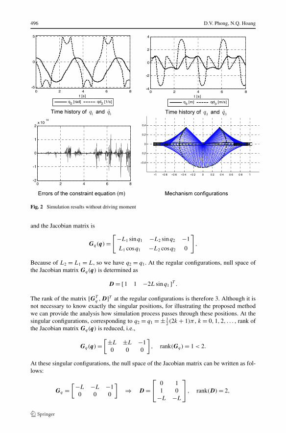
Because of L2 = L1 = L, so we have q2 = q1. At the regular configurations, null space ofthe Jacobian matrix Gq(q) is determined as
D = [1 1 −2L sinq1 ]T .
The rank of the matrix [GTq ,D]T at the regular configurations is therefore 3. Although it is
not necessary to know exactly the singular positions, for illustrating the proposed methodwe can provide the analysis how simulation process passes through these positions. At thesingular configurations, corresponding to q2 = q1 = ± 1
2 (2k + 1)π , k = 0,1,2, . . . , rank ofthe Jacobian matrix Gq(q) is reduced, i.e.,
Gq(q) =[±L ±L −1
0 0 0
], rank(Gq) = 1 < 2.
At these singular configurations, the null space of the Jacobian matrix can be written as fol-lows:
Gq =[−L −L −1
0 0 0
]⇒ D =
⎡⎣ 0 1
1 0−L −L
⎤⎦ , rank(D) = 2,
Singularity-free simulation of closed loop multibody systems 497
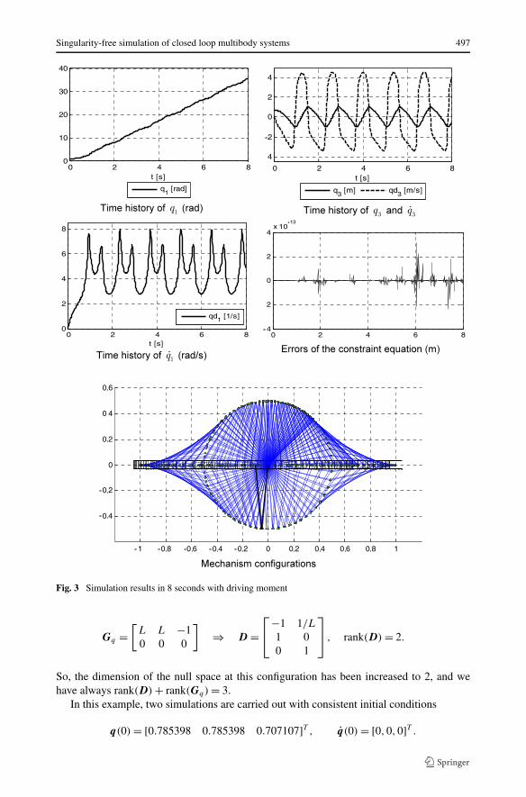
Fig. 3 Simulation results in 8 seconds with driving moment
Gq =[
L L −10 0 0
]⇒ D =
⎡⎣−1 1/L
1 00 1
⎤⎦ , rank(D) = 2.
So, the dimension of the null space at this configuration has been increased to 2, and wehave always rank(D) + rank(Gq) = 3.
In this example, two simulations are carried out with consistent initial conditions
Fig. 4 Simulation results in 20 seconds with driving moment
In the first simulation, there is not applied moment on the crank; the mechanism is forcedto move by only gravity. While in the second case, the mechanism is moved under actingof moment u1 = 10 − 2q1 on the crank OA. The numerical simulation is performed by theRunge–Kutta rule with fixed step time equal to 0.01 s. The scheme for constraint stabiliza-tion is the method of position and velocity projection. The simulation results are shown inthe Figs. 2, 3, and 4.
Simulation results of the first case are shown in the Fig. 2. In this case, the system isconservative. The results show that time history of the generalized coordinates change re-peatedly. The mechanism moves smoothly through the singular configurations and the errorsof the constraint equations hold very small about 10−14 m.
Figures 3 and 4 show the simulation results of the second case. Since there is an appliedmoment on the driving link, the crank OA increases respectively to time. The mechanismmoves also smoothly through the singular configurations and the errors of the constraintequations hold very small about 10−13 m. These small errors are also maintained when theintegration time is set longer, Fig. 4. This confirms the stability of the integration processwith the projection techniques.
Singularity-free simulation of closed loop multibody systems 499
The comparison of two alternative forms: with and without the reaction force vector r
was also provided. The results show that these two forms have practically the same effect.The reduced form seems to be simpler since it consists of fewer equations; however, if thereaction force r is required in direct way it is better to use the original form. The mostimportant for simulation is the using of null space matrix with combination with a goodintegration scheme and stabilization method.
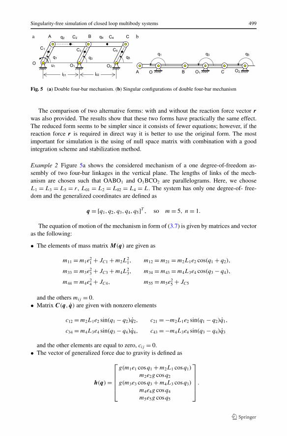
Example 2 Figure 5a shows the considered mechanism of a one degree-of-freedom as-sembly of two four-bar linkages in the vertical plane. The lengths of links of the mech-anism are chosen such that OABO1 and O1BCO2 are parallelograms. Here, we chooseL1 = L3 = L5 = r , L01 = L2 = L02 = L4 = L. The system has only one degree-of- free-dom and the generalized coordinates are defined as
q = [q1, q2, q3, q4, q5]T , so m = 5, n = 1.
The equation of motion of the mechanism in form of (3.7) is given by matrices and vectoras the following:
• The elements of mass matrix M(q) are given as
m11 = m1e21 + JC1 + m2L
21, m12 = m21 = m2L1e2 cos(q1 + q2),
m33 = m3e23 + JC3 + m4L
23, m34 = m43 = m4L3e4 cos(q3 − q4),
m44 = m4e24 + JC4, m55 = m5e
25 + JC5
and the others mij = 0.• Matrix C(q, q) are given with nonzero elements
and the other elements are equal to zero, cij = 0.• The vector of generalized force due to gravity is defined as
h(q) =
⎡⎢⎢⎢⎢⎣
g(m1e1 cosq1 + m2L1 cosq1)
m2e2g cosq2
g(m3e3 cosq3 + m4L3 cosq3)
m4e4g cosq4
m5e5g cosq5
⎤⎥⎥⎥⎥⎦ .
500 D.V. Phong, N.Q. Hoang
The constraint equations are given for two closed loops as
g1 = L1 cosq1 + L2 cosq2 − L3 cosq3 − L01 = 0,
g2 = L1 sinq1 + L2 sinq2 − L3 sinq3 = 0,
g3 = L3 cosq3 + L4 cosq4 − L5 cosq5 − L02 = 0,
g4 = L3 sinq3 + L4 sinq4 − L5 sinq5 = 0.
The Jacobian matrix is given as
Gq(q) =
⎡⎢⎢⎢⎣
−L1 sinq1 −L2 sinq2 L3 sinq3 0 0
L1 cosq1 L2 cosq2 −L3 cosq3 0 0
0 0 −L3 sinq3 −L4 sinq4 L5 sinq5
0 0 L3 cosq3 L4 cosq4 −L5 cosq5
⎤⎥⎥⎥⎦ .
In case of L1 = L3 = L5 = r , L01 = L2; L02 = L4, we have
Gq(q) =
⎡⎢⎢⎢⎣
−r sinq1 −L2 sinq2 r sinq3 0 0
r cosq1 L2 cosq2 −r cosq3 0 0
0 0 −r sinq3 −L4 sinq4 r sinq5
0 0 r cosq3 L4 cosq4 −r cosq5
⎤⎥⎥⎥⎦ .
With the chosen length of linkages, the mechanism has singular configurations at q1 =±kπ , k = 0,1,2, . . . . At regular positions q1 �= ±kπ , k = 0,1,2, . . . , the Jacobian matrixGq(q) has a full rank, equal to 4. And the null space in this case is
D = [1 0 1 0 1]T .
And the rank of the matrix [GTq ,D]T is 5. Again for illustration, we can check the situation
at singular configurations. At positions q1 = ±kπ , k = 0,1,2, . . . q5 = q3 = q1, q4 = q2 =±kπ , rank of Gq(q) reduces and is equal to two
Gq =
⎡⎢⎢⎣
0 0 0 0 0±r L2 ∓r 0 00 0 0 0 00 0 ±r L4 ∓r
⎤⎥⎥⎦ , rank(Gq) = 2 < 4.
At these singular configurations, the null space of the Jacobian matrix can be written asfollows:
Gq =
⎡⎢⎢⎣
0 0 0 0 0r L2 −r 0 00 0 0 0 00 0 r L4 −r
⎤⎥⎥⎦ ⇒ D =
⎡⎢⎢⎢⎢⎣
−L2/r −L4/r 11 0 00 −L4/r 10 1 00 0 1
⎤⎥⎥⎥⎥⎦ , rank(D) = 3,
Gq =
⎡⎢⎢⎣
0 0 0 0 0−r L2 r 0 00 0 0 0 00 0 −r L4 r
⎤⎥⎥⎦ ⇒ D =
⎡⎢⎢⎢⎢⎣
1 0 00 1 01 −L2/r 00 0 11 −L2/r −L4/r
⎤⎥⎥⎥⎥⎦ , rank(D) = 3.
Singularity-free simulation of closed loop multibody systems 501
Fig. 6 Simulation results
So, the rank of the null space at these configurations has been increased to 3, and we havealways rank(D) + rank(Gq) = 5.
Following are the system parameters used in simulations:
In this example, a simulation is performed with initial conditions of driving link of q1(0) =80◦, q1(0) = 0. Solving constraint equations, one obtains the consistent initial conditions asfollows:
In this example, there is not driven moment acting on the mechanism. The integrationstep is chosen as constant with �t = 0.01 s and the Runge–Kutta rule is used in the simula-tion.
The simulation is performed in time interval of 8 s. The results obtained are displayed inFig. 6. The left column plot shows the time history of the coordinates q1, q3, q5 from top tobottom. The right column shows the q2, errors of constraint equations, and the mechanismconfigurations of in the first second respectively. During the simulation, the mechanism goesthrough the singular positions (q1 = ±kπ ) 6 times with no difficulty and without lockingthe simulation. The results show that there are no differences between of the time history ofthe coordinates q1, q3, q5.
It is worth to make a remark that in our examples the problems can be solved with the in-dependent generalized coordinates; however, the described technique with redundant gener-alized coordinates is very general and can be applied to any multibody system in comparisonwith the concept of minimal number of generalized coordinates.
5 Conclusion
In this paper, a new form of equation of motion for constrained systems is presented byintroducing the generalized reaction forces. The null space of Jacobian matrix is exploitedto close the set of equations for the system. The most important advantage of this new formis that the numerical simulation can be performed smoothly through the singular configura-tions. The post-adjusting technique is also applied to guarantee the constraints in the systemfrom breakdown as well. Numerical experiments have been shown to verify the efficienciesof the proposed approach.
References
1. Amirouche, F.M.L., Tung, C.-W.: Regularization and stability of the constraints in the dynamics of multi-body systems. Nonlinear Dyn. 1(6), 459–475 (1990)
2. Bauchau, O.A., Laulusa, A.: Review of contemporary approaches for constraint enforcement in multi-body system. J. Comput. Nonlinear Dyn. 3, 011005 (2008)
3. Baumgarte, J.: Stabilization of constraints and integrals of motion in dynamical systems. Comput. Meth-ods Appl. Mech. Eng. 1, 1–16 (1972)
4. Bayo, E., Avello, A.: Singularity-free augmented Lagrangian algorithms for constrained multibody dy-namics. Nonlinear Dyn. 5, 209–231 (1994)
5. Bayo, E., Ledesma, R.: Augmented Lagrangian and mass-orthogonal projection methods for constrainedmultibody dynamics. Nonlinear Dyn. 9, 113–130 (1996)
6. Bayo, E., Jalon, J.G., Serna, M.A.: A modified Lagrangian formulation for the dynamic analysis ofconstrained mechanical systems. Comput. Methods Appl. Mech. Eng. 71, 183–195 (1988)
7. Blajer, W., Schiehlen, W., Schirm, W.: A projective criterion to the coordinate partitioning method formultibody dynamics. Arch. Appl. Mech. 64, 215–222 (1994)
8. Blajer, W.: Elimination of constraint violation and accuracy aspects in numerical simulation of multibodysystems. Multibody Syst. Dyn. 7, 265–284 (2002)
Singularity-free simulation of closed loop multibody systems 503
9. Braun, D.J., Goldfarb, M.: Eliminating constraint drift in the numerical simulation of constrained dy-namical systems. Comput. Methods Appl. Mech. Eng. 198(37–40), 3151–3160 (2009)
10. Eich, E.: Convergence results for a coordinate projection method applied to mechanical systems withalgebraic constraints. SIAM J. Numer. Anal. 30, 1467–1482 (1993)
11. Ider, S.K., Amirouche, F.M.L.: Coordinate reduction in constrained spatial dynamic systems—a newapproach. J. Appl. Mech. 55, 899–905 (1988)
12. Ider, S.K., Amirouche, F.M.L.: Numerical stability of the constraints near singular positions in the dy-namics of multibody systems. Comput. Struct. 33, 129–137 (1989)
13. Jalon, J.G., Bayo, E.: Kinematic and Dynamic Simulation of Multibody Systems—The Real-Time Chal-lenge. Springer, New York (1994)
14. Kamman, J.W., Huston, R.L.: Dynamics of constrained multibody systems. J. Appl. Mech. 51, 899(1984)
15. Kane, T.R., Levinson, D.A.: Dynamics: Theory and Applications. McGraw-Hill, New York (1985)16. Lin, S.T., Huang, J.N.: Stabilization of Baumgarte’s method using the Runge–Kutta approach. J. Mech.
Des. 124(4), 633 (2002)17. Meyer, C.D.: Matrix Analysis and Applied Linear Algebra. SIAM, Philadelphia (2001)18. Murray, R.M., Li, Z., Sastry, S.S.: A Mathematical Introduction to Robotic Manipulation. CRC Press,
Boca Raton (1994)19. Nikravesh, P.E.: Some methods for dynamic analysis of constrained mechanical systems: a survey. In:
Haug, E.J. (ed.) Computer-Aided Analysis and Optimization of Mechanical System Dynamics, pp. 351–368. Springer, Berlin (1984)
21. Orden, J.C.G., Ortega, R.A.: A conservative augmented Lagrangian algorithm for the dynamics of con-strained mechanical systems. In: The Third European Conference on Computational Mechanics (2006)
22. Petzold, L.R., Ren, Y., Maly, T.: Regularization of higher-index differential-algebraic equations withrank-deficient constraints. SIAM J. Sci. Comput. 18, 753–774 (1997)
23. Phong, D.V.: Principle of compatibility and criteria of ideality in study of constrained mechanical sys-tems. Stroj. cas. 47(1), 2–11 (1996)
24. Phong, D.V.: An algorithm for deriving equations of motion of constrained mechanical system. J. Mech.,NCNST Vietnam 21(1), 36–44 (1999)
25. Schiehlen, W. (ed.): Multibody System Handbook. Springer, Heidelberg (1990)26. Schiehlen, W.: Multibody system dynamics: roots and perspectives. Multibody Syst. Dyn. 1, 149–188
(1997)27. Shabana, A.A.: Dynamics of Multibody Systems, 2nd edn. Cambridge University Press, Cambridge
(1998)28. Terze, Z., Lefeber, D., Muftic, O.: Null space integration method for constrained multibody system
simulation with no constraint violation. Multibody Syst. Dyn. 6, 229–243 (2001)29. Terze, Z., Naudet, J.: Geometric properties of projective constraint violation stabilization method for
generally constrained multibody systems on manifolds. Multibody Syst. Dyn. 20, 85–106 (2008)30. Terze, Z., Naudet, J.: Structure of optimized generalized coordinates partitioned vectors for holonomic


![0-( & & & & & 1+2(3&44444444444444444444444444444 · !"# $$%&'()*(+&,$$-./.011$2$ [ \ ] 6 $ $ $ $ $ !3# $$$-./.011$2$ ^ _ ` a b #$$4567$-.01$867$/.01# $!!! 5 2 4 3 I 1 fF4 gu fC2](https://static.documents.pub/doc/80x56/5ec3c5f3a76875481d64f0c8/0-12344444444444444444444444444444-.jpg)


