10
10.2 The Multinomial Distribution Ulrich Hoensch Monday, April 08, 2013

10.2 The Multinomial Distribution
Ulrich Hoensch
Monday, April 08, 2013

The Multinomial SettingA probability experiment consists of selecting an object at randomfrom exactly one of k bins, where the probability of selecting theobject from the ith bin is pi . Suppose the experiment is repeated ntimes independently. Let Xi be the random variable that givesthe number of objects selected from the ith bin.
In this situation, we say that the random vector (X1,X2, . . . ,Xk)has a multinomial distribution. Note that for k = 2, we obtain abinomial distribution.
Theorem 10.2.1
If (X1,X2, . . . ,Xk) has a multinomial distribution, then
P(X1 = x1, . . . ,Xk = xk) =
(n
x1 x2 . . . xk
)px11 px22 . . . pxkk
=n!
x1!x2! . . . xk !px11 px22 . . . pxkk .

Example
Suppose five observations are independently obtained from thedistribution with PDF
f (x) = 6x(1 − x), 0 ≤ x ≤ 1.
Find the probability that one observation lies in the interval[0, 0.25), none in the interval [0.25, 0.50), three in the interval[0.50, 0.75), and one in the interval [0.75, 1].
We have 4 bins, and the probability for each bin can be obtainedby integration. For example,
p1 =
∫ 0.25
06x(1 − x) dx =
5
32.
Example
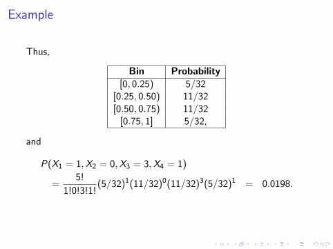
Thus,
Bin Probability[0, 0.25) 5/32
[0.25, 0.50) 11/32[0.50, 0.75) 11/32
[0.75, 1] 5/32,
and
P(X1 = 1,X2 = 0,X3 = 3,X4 = 1)
=5!
1!0!3!1!(5/32)1(11/32)0(11/32)3(5/32)1 = 0.0198.
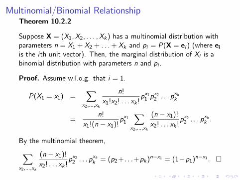
Multinomial/Binomial RelationshipTheorem 10.2.2
Suppose X = (X1,X2, . . . ,Xk) has a multinomial distribution withparameters n = X1 + X2 + . . . + Xk and pi = P(X = ei ) (where ei
is the ith unit vector). Then, the marginal distribution of Xi is abinomial distribution with parameters n and pi .
Proof. Assume w.l.o.g. that i = 1.
P(X1 = x1) =∑
x2,...,xk
n!
x1!x2! . . . xk !px11 px22 . . . pxkk
=n!
x1!(n − x1)!px11
∑x2,...,xk
(n − x1)!
x2! . . . xk !px22 . . . pxkk .
By the multinomial theorem,∑x2,...,xk
(n − x1)!
x2! . . . xk !px22 . . . pxkk = (p2+ . . .+pk)n−x1 = (1−p1)n−x1 . �

Example
Suppose 32 independent selections from 4 bins resulted in thefollowing observed frequencies:
Bin Obs. Freq.1 102 53 104 7
Suppose we assume that a multinomial distribution with(p1, p2, p3, p4) = (5/32, 11/32, 11/32, 5/32) applies. We formulatethe null hypothesis
H0 : p1 = 5/32, p2 = 11/32, p3 = 11/32, p4 = 5/32.
We want to compute the probabilty that under H0, the observedfrequencies or more extreme frequencies occur. This is the(exact) p-value for H0.

Example
This leads to the following table.
Bin Obs. Freq. Exp. Freq. Difference1 10 5 52 5 11 63 10 11 14 7 5 2
The range R for the observed and more extreme frequences is:
I X1 : 0, 10 − 32
I X2 : 0 − 5, 17 − 32
I X3 : 0 − 10, 12 − 32
I X4 : 0 − 3, 7 − 32
Note that we also need X1 + X2 + X3 + X4 = 32.

Example
The exact p-value is
p =∑
(x1,x2,x3,x4)∈R
32!
x1!x2!x3!x4!
(5
32
)x1 (11
32
)x2 (11
32
)x3 ( 5
32
)x4
≈ 0.0008 = 0.08%.
Thus, we reject the null hypothesis that the given multinomialdistribution applies. The p-value was computed using the followingMathematica code.
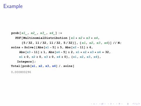
Example
prob@x1_, x2_, x3_, x4_D :=
PDF@MultinomialDistribution @x1 + x2 + x3 + x4,
85 � 32, 11 � 32, 11 � 32, 5 � 32<D, 8x1, x2, x3, x4<D �� N;
solns = Solve@8Abs@x1 - 5D ³ 5, Abs@x2 - 11D ³ 6,
Abs@x3 - 11D ³ 1, Abs@x4 - 5D ³ 2, x1 + x2 + x3 + x4 � 32,
x1 ³ 0, x2 ³ 0, x3 ³ 0, x4 ³ 0<, 8x1, x2, x3, x4<,
IntegersD;
Total@prob@x1, x2, x3, x4D �. solnsD0.000800296

Homework Problems for Section 10.2 (Points)
p.498-499: 10.2.2 (2), 10.2.8 (2).
Homework problems are due at the beginning of the class onMonday, April 15, 2013.


