1.2 Heat transfer from electrical equipment - EE&T Lecture ... - Lec2 - Heat... · 1.2 Heat...

ELEC9712: Heat Transfer p. 1/32

ELEC9712 High Voltage Systems

1.2 Heat transfer from electrical equipment

The basic equation governing heat transfer in an item of electrical equipment is the following incremental balance equation, with dθ and dt being incremental changes in temperature and time respectively:

( )0pPdt m c d Ah T T dtθ= × + −

where: P = power dissipation (generation) level in the

equipment

m = equipment mass

cp = specific heat of the equipment material

h = overall heat dissipation coefficient

A = surface area available for heat dissipation from equipment

T = surface temperature

To = ambient temperature

Thus • Pdt is the energy dissipation in time dt • dθ is the temperature rise of the equipment in dt • pmc is the thermal capacity of the equipment • ( )0Ah T T− is the heat dissipated to the ambient in dt.


Under steady state heating conditions, we have constant temperature θ, and so

( )0Pdt Ah T T dt= −

This equation is the basis for determination of continuous thermal rating of equipment. Under short circuit conditions, the heating is adiabatic

( ) 0oh T T − = and thus we have

pPdt mc dθ=

This equation is the basis for determining transient rating of electrical equipment. We will look at these two cases separately. Steady state heating and thermal transfer Cooling of electrical equipment is usually achieved by a combination of the three standard modes of heat transfer mechanisms, viz. conduction, convection and radiation. In order to quantify the actual heat transfer rates by any of the above mechanisms or combination of mechanisms, a number of material and configuration (geometrical) factors must be taken into account. These include the following important parameters:


A surface area of equipment cp specific heat of the major material involved k thermal conductivity of the material ρ material density ε radiative emissivity of the surface β expansion coefficient of the material being heated v fluid flow velocity past hot surfaces µ fluid viscosity (dynamic) L (or X) a characteristic length of the surface dissipating heat For determining the overall heat transfer rate for an item of equipment under steady state conditions, we must determine an overall heat transfer coefficient h (W/m2/oC), such that the total heat dissipation Ht from the equipment surface is:

( )0t tH Ah T T= − watts where Ht (and thus ht) are the total dissipation including all mechanisms. The determination of ht is very important for any electrical equipment and its calculation must take account of the environment and the equipment considered together. The calculation of ht is achieved by a simple addition of the three individual coefficients for conduction, convection and radiation, or whichever ones are applicable.

t cond conv rh h h h= + + W/m2/oC


The determination of the heat transfer coefficient for conduction is relatively simple. For the radiation coefficient, it is also relatively simple. However, it is very complex for the thermal convection dissipation coefficient. We must develop methods for calculating them according to the following methods:

(i) thermal conduction, using Newton’s law of cooling (ii) thermal radiation, using Stefan’s law emission (iii) thermal convection:

a. natural convection empirical equations b. forced convection empirical equations

1.2.1 Thermal Conduction This is generally the most inefficient method of the three, as most materials that have to dissipate the heat in electrical equipment are electrical insulators and these are also generally good thermal insulators and poor thermal conductors. However, in some cases thermal conduction may be the only dissipation mechanism available (for example in power cables). Thermal conduction is only significant for solid materials: in liquids and gases, convection loss will be much more efficient and dominant than conduction loss.

dH dHA A T1

T2

l

dx

dAdH dHA A T1

T2

l

dx

dA


We are mainly interested in steady state heat conduction, where we can write:

dTdH k dAdx

= − ⋅ H dTkA dx

= −

i.e. ( )2 1kAH T Tl

= − watts

or: ( )2 1AH T Tgl

= −

where: 1gk

= = thermal resistivity

i.e. ( )2 1T T

HG−

=

where: glGA

= = thermal resistance

This is the Thermal Ohm’s Law and the analogy with the electrical Ohm’s law is obvious, with the following correspondence:

H → heat flow → flux quantity → (cf current I) ( )2 1T T− → temperature difference → potential quantity

→ (cf voltage difference V) G → thermal resistance → medium characeristic →

(cf electrical resistance R) We can devise thermal equivalent circuits that can be handled by exact analogy with electrical circuits once the thermal


resistances are determined for the materials and the configurations involved in the equipment. Example:

≡

G1 G2 G3H H

T1 T2 T3 T4A

L1 L2 L3

G1 G2 G3H HT1 T2 T3 T4

≡

G1 G2 G3H H

T1 T2 T3 T4A

L1 L2 L3

G1 G2 G3H HT1 T2 T3 T4

We have:

1 11

g LGA

= ; 2 22

g LGA

= ; 3 33

g LGA

=

and: [ ]1 4 1 2 3T T H G G G− = + + Example:

≡

H H

G1

G2

G3H H

1234

56

7

G4

G5

G6

G7

≡

H H

G1

G2

G3H H

1234

56

7

G4

G5

G6

G7


Calculation of the thermal resistance. G can be calculated using exactly the same methods as are used to determine the electrical resistance for the same geometry. The only change needed is to use the thermal resistivity ( )1g k= instead of the electrical resistivity ρ. For example, for a coaxial geometry, the two equations for electrical and thermal resistance for radial electrical current and heat flow through the cable insulation are:

r a=r b=r a=r b=

ln2

bRa

ρπ

=

(electrical) ohms

ln2g bG

aπ =

thermal ohms

For any thermal insulation geometry we can determine the thermal resistance by using the electrical-thermal analogy so that we can simply use the known electrical resistance expression for any geometry to calculate the thermal resistance. This is done simply by replacing ρ by g. All that is required is the value of thermal resistivity, g.


The most common area of use of thermal resistance is in the rating calculation of power cables, where the above coaxial geometry is used. It is also possible to use the standard line to plane electrical resistance formula for determining the effective thermal resistance between a buried cable to the ground surface above (representing the ambient infinite heat sink). Some typical thermal resistivities (g) of various materials are:

Material g (oCm/W) PVC insulation Mica Porcelain & Glass Moist soil Asphalt Sand (dry) (moist) Air Concrete Rubber Water Oil-paper Wood Polyethylene Copper

7.0 2.0 1.0 1.0 1.4 3.0 0.9 41 1.0 5.0 1.7 6.0

4 – 8 4.0

0.002 Conduction heat transfer coefficient [ ]condh The general equation heat transfer equation is:


( )2 1condH h A T T= − For thermal conduction along a constant cross-section tube of length L,

( )2 1AH T T

gL= − [Th. resistance G gL A= ]

Thus:

1condh

gL= W/m2/oC [g is thermal resistivity]

For most thermal conduction calculations, hcond is not much used as Hcond can be calculated easily from the thermal equivalent circuit. Also, thermal conduction usually acts by itself, so that hconv and hr are not relevant. 1.2.2 Thermal Convection Heat transfer from a surface by a fluid (liquid or gas) by either natural or forced convection flow dissipation depends on the following factors: • Surface temperature • Length of surface exposed to the fluid flow • Surface configuration (shape) • Surface texture (rough or smooth) • Properties of the fluid, particularly the following

o Thermal conductivity k o Density ρ


o Specific heat cp o Viscosity µ o Thermal expansion coefficient β

The first three of the above fluid properties define the thermal diffusivity ( )pk cρ of the fluid which is the main thermal characteristic of importance for convection heat removal from surfaces. As before, we need to find a heat transfer coefficient hconv for dissipation by convection. This is a very complex calculation (estimation!) for convection because the processes involved are not able to be quantified analytically. Empirical equations must be used to determine Hconv and hconv. Empirical equations are available for most commonly encountered surfaces, but for more complex situations we must use a more basic empirical fluid flow approach in the estimation, using the various defined “numbers” to calculate heat transfer. Empirical equations for hcond from typical surfaces are given below. A Natural Convection The method of natural convection flow establishment is the expansion of the fluid as it heats up, thus leading to a reduction in density and hence rising buoyancy forces that cause the hot fluid to rise and be replaced by cooler fluid at the bottom. The following give empirical equations for the


heat transfer coefficients by such a process in simple geometries.

Dissipation from flat surfaces and cylinders by natural convection (a) Vertical plates and cylinders in air

0.25

1.37 ThL∆ =

W/m2/oC [L = plate length]

(b) Horizontal plate in air (top surface)

0.25

1.32 ThL∆ =

W/m2/oC

(c) Horizontal plate in air (bottom surface)

0.25

0.59 ThL∆ =

W/m2/oC

(d) Horizontal cylinder (in air)

0.25

1.32 ThD∆ =

W/m2/oC [D = diameter]

(e) Vertical plate & cylinder in water at 21oC

0.25

127 ThL∆ =

W/m2/oC

(f) Vertical plate & cylinder in transformer oil at 21oC


0.25

59 ThL∆ =

W/m2/oC

Note that in all of the above expressions the heat transfer coefficient calculated will be temperature dependent. This is a significant complication in determining the total heat transfer using the equation, H hA T= ∆ watts

= constant ( )5 4A T× ∆ watts compared to thermal conduction, for example, where the heat transfer coefficient h was constant and independent of temperature. A typical magnitude of the natural convection heat transfer coefficient in air at normal operating temperatures is about

hconv ≈ 5 - 6 W/m2/oC Examples of natural convection in electrical equipment include:

• Natural circulation of oil in transformers • Natural air cooling of pipes on transformers • Heat sinks on power semiconductor components • Natural convection from exposed overhead lines and

busbars


B Forced Convection Dissipation from a flat surface by forced convection flow 5.7 4.5convh v= + [for 5v < m/s - laminar flow]

0.87.8convh v= [for 5v > m/s - turbulent flow] or, we can use the following more general formulation:

1 3Re PrmNu C= where Re is the Reynolds number, Nu is the Nusselt Number, Pr is the Prandtl Number, m is a general exponent dependent on the situation, C is a constant. and we then use the equation:

Nu hL k= where k is thermal conductivity, L is a general length. Thus:

( ) 1 3Re Prmconvh k L C=

The calculation becomes even more complex for cylindrical geometries. Techniques to enhance heat dissipation rates from electrical equipment


From the above equations and the parameter dependencies, some simple techniques of enhancing heat dissipation rates from electrical equipment can be determined as follows:

(a) Natural convection

• Optimisation of surface orientation • Increasing the surface area for dissipation • Use of a fluid with high thermal diffusivity • Keeping ambient temperature low

(b) Forced convection

• Use a high flow velocity • Optimise surface orientation • Use a large surface area • Use a fluid with high thermal diffusivity • Using low ambient temperature

Thermal convection dissipation requires the removal of heat from a hot surface by using fluid flow past the surface to remove heat and dissipate it by the fluid flow. This requires of course that the fluid temperature is kept lower than that of the surface. Such fluid flow past a surface results in a boundary layer of the fluid adhering to the surface with the inner part of the boundary layer at the surface being attached to the surface and essentially static. The fluid velocity then increases in the layer as away from the surface.


The result of this layer attachment is that the thermal transfer then has to take place via the boundary layer, so that even thermal conduction in the fluid material is important in convection dissipation, with the initial transfer being by thermal conduction through the attached static inner fluid layer. Thus convection dissipation is determined by fluid parameters such as the viscous drag of the fluid at the surface, the specific heat of the fluid, the thermal conductivity of the fluid, the viscous drag of the fluid, the fluid flow velocity, fluid density, etc, as well as the thickness of the layer. All of these factors are incorporated in a series of characteristic numbers derived by dimensional analysis of fluid flow and these are used in fluid flow problems to determine general convective dissipation. The following gives a general discussion of the use of such numbers.

Use of non-dimensional characteristic numbers to describe and calculate

convective heat dissipation from surfaces In less well-defined geometries than those for the equations given previously, we have to use the non-dimensional fluid flow numbers to quantify the heat dissipation coefficient.


The fluid flow numbers of importance for convection dissipation are:

The Reynolds Number [ Re ] The Grashof Number [ Gr ] The Prandtl Number [ Pr ] The Nusselt Number [ Nu ]

Reynolds Number (Re)

Re vX vXρµ υ

= =

ρ = fluid density, v = fluid flow velocity, µ = fluid (dynamic) viscosity, υ ( )µ ρ= = kinematic viscosity, and X is some characteristic length. The Reynolds number represents the ratio of the fluid dynamic forces ( ρv2 ) of the flow to the viscous drag forces ( )v Xµ retarding the fluid flow motion. The magnitude of Re indicates whether the flow is laminar or turbulent, giving a numerical criterion for laminar flow. Laminar or turbulent flow is an important factor in determining the convective dissipation of heat by a fluid. The Reynolds number relates primarily to forced flow situations. It is not easy to define a specific Re value for the transition from laminar to turbulent flow, however a value of Re = 105


is often used for general flow conditions, but the geometry will affect this transition value. Thus Laminar flow Re < 105 Turbulent flow Re ≥ 105

A low Re means that viscous forces dominate the flow. A high Re means that inertial forces dominate the flow. Typical values of Re:

For cylindrical pipes, the flow is turbulent when Re ≥ 2000.

For a pipe of diameter 10 mm, and a flow velocity of 10 mm/s:

Re = 6 for air Re = 100 for water Re = 1 for oil

Grashof Number ( Gr )

2 3

2

g XGr Tβρµ

= ⋅∆

g = the gravitational acceleration constant, β = coefficient of volume thermal expansion, T∆ = the temperature difference between the surface and the fluid. Other symbols are as previously defined.


The Grashof number represents the ratio of the fluid buoyancy force of natural convection heat dissipation to the viscous drag of the fluid flow. It represents the effects of the hydrostatic natural buoyancy lift force of the heated fluid and the viscous force opposing the flow during natural convection. Gr is used instead of Re when the convection is naturally generated in the fluid.

Laminar flow Gr < 105 Turbulent flow Gr ≥ 105

Typical values of Gr: For a surface with X = 20 mm, and for a temperature difference T∆ = 10oK

Gr = 7500 for air Gr = 240,000 for water Gr = 20 for oil.

Prandtl Number ( Pr )

pcPr

kµ

=

cp = fluid specific heat, k = fluid thermal conductivity, µ = viscosity. The Prandtl number represents the ratio of momentum diffusivity( )µ ρ of the flow to the thermal diffusivity


( )pk cρ . Note that it does not involve any geometry factors: it is a purely physical property of the fluid. It represents the efficiency relationship of the heat transfer process of the fluid to the fluid motion during convective loss processes. Typical values:

Pr = 0.7 in air Pr = 6.5 in water Pr = 500 in oil Nusselt Number ( Nu )

hXNuk

=

h = convective heat dissipation coefficient of the fluid flow (ultimately this is what we need to calculate to determine heat loss) and k = thermal conductivity of the fluid. The Nusselt number is the basic parameter which quantifies convective heat transfer by a fluid. It represents the ratio of convective heat transfer ( )hA T∆ to conductive heat transfer ( )kA T X∆ by the fluid. In order to find h, the Nusselt number must be evaluated from the Re, Gr and Pr numbers (as appropriate to the flow conditions). The Re, Gr and Pr numbers are themselves determined from the fluid properties


and the geometry using experimental data for various fluids and geometries. We use the following form of relationship: Nu = f (Gr, Pr ) for natural convection

Nu = f1( Re, Pr ) for forced convection The functional nature of f and f1 are determined by the situation and fluid properties. For natural convection, Nu ∝ Gr1/4 for laminar flow

Nu ∝ Gr1/3 for turbulent flow For forced convection, Nu ∝ Re1/2 for laminar flow

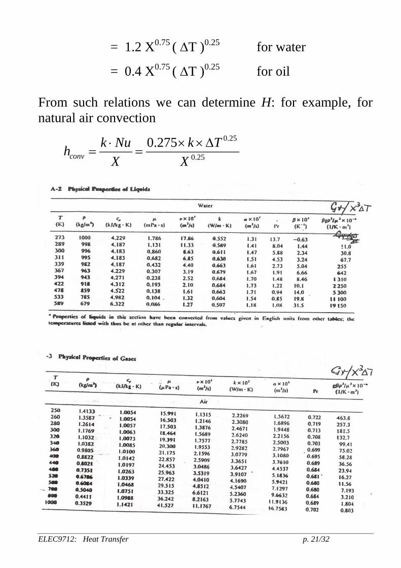
Nu ∝ Re4/5 for turbulent flow For natural convection the following equation is often used: Nu = 0.53 ( Gr. Pr)0.25 = 0.275 X0.75 ( ∆T )0.25 for air


= 1.2 X0.75 ( ∆T )0.25 for water

= 0.4 X0.75 ( ∆T )0.25 for oil From such relations we can determine H: for example, for natural air convection

0.25

0.25

0.275conv

k Nu k ThX X⋅ × ×∆

= =




1.2.3 Thermal radiation All bodies radiate electromagnetic radiation. At normal temperatures under consideration here, [T ≈ 100oC or 373oK] this radiation is primarily in the infra-red region of the spectrum. For a body at an absolute temperature of T kelvin, the heat radiated is given by Stefan’s Law:

4H Tσε= W/m2 where: σ is Stefan’s constant (5.7 x 10-8 W/m2K4) ε is the surface radiative emissivity (0 < ε ≤ 1) T is the absolute temperature of the surface [K] However at the same time as radiating heat, the body will also absorb heat from the ambient, which is at temperature T0 oK, so that the net quantity of heat lost by the body at T oK will be given by:

4 40H T T Aσε = − watts

where T is the surface temperature (oK) T0 is the ambient temperature (oK) Here we assume that the radiation absorption coefficient of the surface is the same as the emissivity coefficient. This is generally a good assumption, though not always strictly correct.


The value of emissivity ε is very dependent on the surface condition:

ε ≈ 0.8 – 0.9 for a matt (eg weathered) surface ε ≈ 0.2 – 0.3 for a shiny (eg new) surface We can calculate from the above an expression for the radiative heat transfer coefficient hr, using the usual general expression

[ ]r oH h A T T= − watts We get: [ ] 2 2

r o oh T T T Tσε = + + W/m2/oC It can be seen that, as with the convective heat transfer coefficient, the radiative heat transfer coefficient is also temperature dependent. Typically, hr is about 4 - 6 W/m2/oK at normal operating temperatures. At normal operating temperatures we can approximate hr by the expression:

( )0.172.9r oh T Tε= − W/m2/oK For example,

for T = 333 oK, To = 293 oK and ε = 0.8 the heat transfer coefficient is:

( )0.172.9 0.8 40 4.3rh = × × ≈ W/m2/oK


1.2.4 Examples of calculations (a) Temperature distribution in a transformer winding:

Heat flow

transformercore

Heat flow

transformercore

The winding has three layers of insulated copper as shown. The space factor = 0.75 = (area of copper) / (total area) The 2I R loss = 17.8 W/kg in the winding. The thermal resistivity of the insulation over the copper is g = 7.5 oKm/W. The total thickness of the three layers = 30 mm. It is required to find the temperature distribution across the winding. Assume no core loss.

x

1

yx

1

y


The space factor = 0.75, i.e. if the insulation thickness is y and the copper area is x2, with total side taken as unity:

2

2 0.751x

= ⇒ 0.866x = units, and 2 0.134y = units

The insulation covers 1 0.134x− = of the overall thickness. To calculate thermal transfer and temperature rise (fall) we need an effective thermal resistivity of the copper and insulation.

( )1eff insg g x= − [assume 0cug = ] ( )7.5 1 0.866 1.01= × − = oKm/W If power loss = p watts/m3 then in the volume ( )1 1 x× × :

loss px= watts This flows radially from left to right

x= 0 x= a

x

dTdx

x= 0 x= a

x

dTdx

Hence: ( )1 1effg dx

dT px=×

oK


effpx g dx= ⋅ ⋅

and: 0

a

T dT∆ = ∫

2

0

12

a

eff effpg xdx g pa= =∫ oK above ambient

where: p = space factor x Cu density x 17.8 W/m3

( )3 50.75 8.9 10 17.8 1.19 10= × × × = × W/m3 1.01effg = 0.03a = m Hence:

( )5 21 1.01 1.19 10 0.03 542

T∆ = × × × × = oK

and the variation is parabolic.

x0 x = a

To

54oK

T

x0 x = a

To

54oK

T

(b) Loss calculation for a transformer: Transformer is oil-filled with circulation of oil through pipes mounted on walls.


oil flowoil flow

There are 2 heat loss mechanisms: radiation and convection. The transformer rating is 7.5 MVA and has a rated core loss = 14 kW and copper loss = 46 kW. Total = 60 kW. The tank is 1.4m x 2.5m x 3.0m high. It has 925m of external tubes to circulate oil. Tube diameter = 50mm. Determine the average surface temperature rise above 25oC ambient for rated current. Assume 0.9ε = for all surfaces and:

For flat top surface 0.252.6convh T= ×∆ W/m2/K For vertical surface 0.252.0convh T= ×∆ W/m2/K For vertical pipes 0.25 0.251.3convh d T−= ∆ W/m2/K (i) Radiation loss

( )4 4298r surfp Tσε= − W/m2

( ) ( )8 4 45.7 10 0.9 298surfT−= × × × − and: r rP p A=


In this case, A is the effective area presented to the ambient.

A = top surface + 4 sides

1.4 2.5 2 1.4 3 2 2.5 3 26.9= × + × × + × × = m2 Thus: 6 4 41.38 10 298r surfP T− = × − watts (ii) Convection loss

Top surface: ( )1 42.6 25h θ= × − W/m2/K

( )5 42.6 25p θ= × − W/m2 A = 3.5 m2

( )5 49.1 25topP θ= × − watts Flat sides:

( )1 42.0 25h θ= × − W/m2/K

( )5 42.0 25p θ= × − W/m2 A = 23.4 m2

( )5 446.8 25sidesP θ= × − watts Tubes:

( ) ( )1 4 1 41.3 0.05 25h θ−= × × − W/m2/K

( ) ( )1 4 5 41.3 0.05 25p θ−= × × − W/m2 925 0.05 145.2A π= × × = m2

( )5 4399 25tubesP θ= × − watts


Thus, total loss is:

[ ]( )46 41.38 10 273 298totP θ−= × + −

( )( )5 49.1 46.8 399 25θ+ + + −

[ ]( ) ( )5 446 41.38 10 273 298 454.9 25totP θ θ−= × + − + −

= 60 kW Have to solve by iteration. Try 70θ = oC as first trial. Then heat loss: ( ) ( )1.25 6 4 4455 45 1.38 10 343 298−= + × − 53.03 8.22 61.25= + = kW Try 69θ = oC, we get 51.56 8.00 59.56= + = kW

Try 69.2θ = oC, we get 51.71 8.02 59.73= + = kW

Try 69.3θ = oC, we get 52.00 8.06 60.06= + = kW

69.3θ = oC is close enough. Thus the surface temperature is:

69.3 25 44.3θ∆ = − = oC (or oK) above ambient To consider the effect of overloading, we try the calculation assuming a load of 1.25 pu, losses will be:

( )214 46 1.25 85.9+ = kW Apply same iteration procedure. Try 85θ = oC as first trial. Then heat loss:


75.98 11.79 87.77= + = kW Try 84θ = oC, we get 74.40 11.53 85.93= + = kW

84θ = oC is close enough. Thus the temperature rise above ambient is:

84 25 59θ∆ = − = oC (or oK) To consider the effectiveness of the cooling pipes, we try the calculation assuming only the tank sides, i.e.

conv ( )5 455.9 25θ= − with same radiation Try 100θ = oC: 12.34convP = , 15.83rP = , 28.17totP = kW

Try 140θ = oC: 21.05convP = , 29.27rP = , 50.32totP = kW

Try 150θ = oC: 23.36convP = , 33.30rP = , 56.66totP = kW

Try 155θ = oC: 24.54convP = , 35.43rP = , 59.97totP = kW Thus the temperature is 155θ = oC and the temperature rise above ambient is:

155 25 130θ∆ = − = oC (or oK) as compared to 44.3oC with pipes. It can be seen that the pipes provide a significant improvement in cooling.

Date post:	19-May-2018
Category:	Documents
Upload:	phungliem
View:	218 times
Download:	2 times

1.2 Heat transfer from electrical equipment - EE&T Lecture ... - Lec2 - Heat... · 1.2 Heat...

Documents