14-1

Chapter 14Chapter 14

Risk and Managerial Risk and Managerial Options in Capital Options in Capital

BudgetingBudgeting

Risk and Managerial Risk and Managerial Options in Capital Options in Capital

BudgetingBudgeting© 2001 Prentice-Hall, Inc.

Fundamentals of Financial Management, 11/eCreated by: Gregory A. Kuhlemeyer, Ph.D.

Carroll College, Waukesha, WI

14-2

Risk and Managerial Risk and Managerial Options in Capital BudgetingOptions in Capital BudgetingRisk and Managerial Risk and Managerial Options in Capital BudgetingOptions in Capital Budgeting

The Problem of Project Risk

Total Project Risk

Contribution to Total Firm Risk: Firm-Portfolio Approach

Managerial Options

The Problem of Project Risk

Total Project Risk

Contribution to Total Firm Risk: Firm-Portfolio Approach

Managerial Options

14-3

An Illustration of Total An Illustration of Total Risk (Discrete Distribution)Risk (Discrete Distribution)An Illustration of Total An Illustration of Total Risk (Discrete Distribution)Risk (Discrete Distribution)

ANNUAL CASH FLOWS: YEAR 1PROPOSAL APROPOSAL A

State ProbabilityProbability Cash FlowCash Flow

Deep Recession .05 $ -3,000

Mild Recession .25 1,000

Normal .40 5,000

Minor Boom .25 9,000

Major Boom .05 13,000

ANNUAL CASH FLOWS: YEAR 1PROPOSAL APROPOSAL A

State ProbabilityProbability Cash FlowCash Flow

Deep Recession .05 $ -3,000

Mild Recession .25 1,000

Normal .40 5,000

Minor Boom .25 9,000

Major Boom .05 13,000

14-4

Probability Distribution Probability Distribution of Year 1 Cash Flowsof Year 1 Cash FlowsProbability Distribution Probability Distribution of Year 1 Cash Flowsof Year 1 Cash Flows

.40

.05

.25

Pro

bab

ility

-3,000 1,000 5,000 9,000 13,000

Cash Flow ($)

Proposal AProposal A

14-5

CFCF11 PP11 (CFCF11)()(PP11))

$ -3,000 .05 $ -150 1,000 .25 250 5,000 .40 2,000 9,000 .25 2,250 13,000 .05 650

=1.001.00 CFCF11=$5,000$5,000

CFCF11 PP11 (CFCF11)()(PP11))

$ -3,000 .05 $ -150 1,000 .25 250 5,000 .40 2,000 9,000 .25 2,250 13,000 .05 650

=1.001.00 CFCF11=$5,000$5,000

Expected Value of Year 1 Expected Value of Year 1 Cash Flows (Cash Flows (Proposal AProposal A))Expected Value of Year 1 Expected Value of Year 1 Cash Flows (Cash Flows (Proposal AProposal A))

14-6

(CFCF11)()(PP11)) ( (CFCF11 - - CFCF11))22((PP11) )

$ -150 ( -3,000 - 5,000)22 ( (.05.05)) 250 ( 1,000 - 5,000)22 ( (.25.25)) 2,000 ( 5,000 - 5,000)22 ( (.40.40)) 2,250 ( 9,000 - 5,000)22 ( (.25.25)) 650 (13,000 - 5,000)22 ( (.05.05))

$5,000$5,000

(CFCF11)()(PP11)) ( (CFCF11 - - CFCF11))22((PP11) )

$ -150 ( -3,000 - 5,000)22 ( (.05.05)) 250 ( 1,000 - 5,000)22 ( (.25.25)) 2,000 ( 5,000 - 5,000)22 ( (.40.40)) 2,250 ( 9,000 - 5,000)22 ( (.25.25)) 650 (13,000 - 5,000)22 ( (.05.05))

$5,000$5,000

Variance of Year 1 Variance of Year 1 Cash Flows (Cash Flows (Proposal AProposal A))Variance of Year 1 Variance of Year 1 Cash Flows (Cash Flows (Proposal AProposal A))

14-7

Variance of Year 1 Variance of Year 1 Cash Flows (Cash Flows (Proposal AProposal A))Variance of Year 1 Variance of Year 1 Cash Flows (Cash Flows (Proposal AProposal A))

(CFCF11)()(PP11)) ( (CFCF11 - - CFCF11))22*(*(PP11) )

$ -150 3,200,000 250 4,000,000 2,000 0 2,250 4,000,000 650 3,200,000

$5,000$5,000 14,400,00014,400,000

(CFCF11)()(PP11)) ( (CFCF11 - - CFCF11))22*(*(PP11) )

$ -150 3,200,000 250 4,000,000 2,000 0 2,250 4,000,000 650 3,200,000

$5,000$5,000 14,400,00014,400,000

14-8

Summary of Summary of Proposal AProposal A

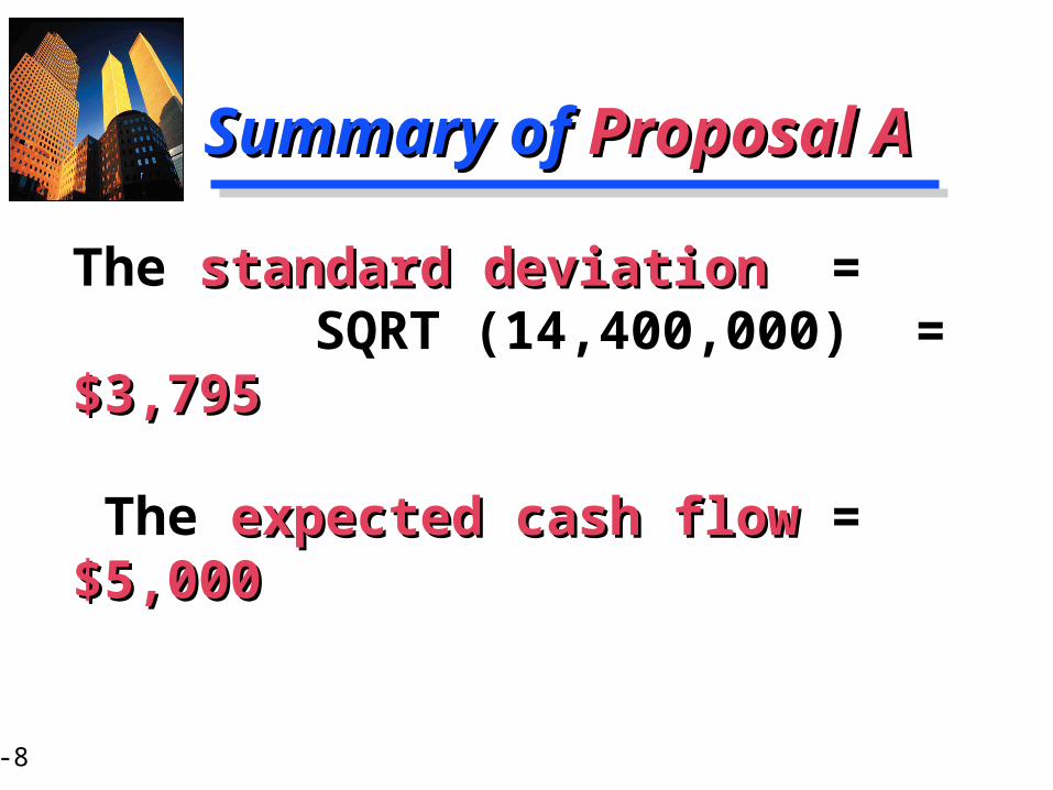
The standard deviation standard deviation = SQRT (14,400,000) = $3,795$3,795

The expected cash flow expected cash flow = $5,000$5,000

14-9

An Illustration of Total An Illustration of Total Risk (Discrete Distribution)Risk (Discrete Distribution)An Illustration of Total An Illustration of Total Risk (Discrete Distribution)Risk (Discrete Distribution)

ANNUAL CASH FLOWS: YEAR 1PROPOSAL BPROPOSAL B

State ProbabilityProbability Cash FlowCash Flow

Deep Recession .05 $ -1,000

Mild Recession .25 2,000

Normal .40 5,000

Minor Boom .25 8,000

Major Boom .05 11,000

ANNUAL CASH FLOWS: YEAR 1PROPOSAL BPROPOSAL B

State ProbabilityProbability Cash FlowCash Flow

Deep Recession .05 $ -1,000

Mild Recession .25 2,000

Normal .40 5,000

Minor Boom .25 8,000

Major Boom .05 11,000

14-10

Probability Distribution Probability Distribution of Year 1 Cash Flowsof Year 1 Cash FlowsProbability Distribution Probability Distribution of Year 1 Cash Flowsof Year 1 Cash Flows

.40

.05

.25

Pro

bab

ility

-3,000 1,000 5,000 9,000 13,000

Cash Flow ($)

Proposal BProposal B

14-11

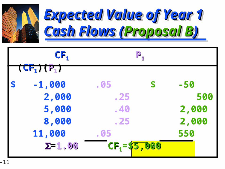
Expected Value of Year 1 Expected Value of Year 1 Cash Flows (Cash Flows (Proposal BProposal B))Expected Value of Year 1 Expected Value of Year 1 Cash Flows (Cash Flows (Proposal BProposal B))

CFCF11 PP11 (CFCF11)()(PP11))

$ -1,000 .05 $ -50 2,000 .25 500 5,000 .40 2,000 8,000 .25 2,000 11,000 .05 550

=1.001.00 CFCF11=$5,000$5,000

CFCF11 PP11 (CFCF11)()(PP11))

$ -1,000 .05 $ -50 2,000 .25 500 5,000 .40 2,000 8,000 .25 2,000 11,000 .05 550

=1.001.00 CFCF11=$5,000$5,000

14-12

(CFCF11)()(PP11)) ((CFCF11 - - CFCF11))22((PP11))

$ -50 ( -1,000 - 5,000)22 ( (.05.05)) 500 ( 2,000 - 5,000)22 ( (.25.25)) 2,000 ( 5,000 - 5,000)22 ( (.40.40)) 2,000 ( 8,000 - 5,000)22 ( (.25.25)) 550 (11,000 - 5,000)22 ( (.05.05))

$5,000$5,000

(CFCF11)()(PP11)) ((CFCF11 - - CFCF11))22((PP11))

$ -50 ( -1,000 - 5,000)22 ( (.05.05)) 500 ( 2,000 - 5,000)22 ( (.25.25)) 2,000 ( 5,000 - 5,000)22 ( (.40.40)) 2,000 ( 8,000 - 5,000)22 ( (.25.25)) 550 (11,000 - 5,000)22 ( (.05.05))

$5,000$5,000

Variance of Year 1 Variance of Year 1 Cash Flows (Cash Flows (Proposal BProposal B))Variance of Year 1 Variance of Year 1 Cash Flows (Cash Flows (Proposal BProposal B))

14-13

Variance of Year 1 Variance of Year 1 Cash Flows (Cash Flows (Proposal BProposal B))Variance of Year 1 Variance of Year 1 Cash Flows (Cash Flows (Proposal BProposal B))

(CFCF11)()(PP11)) ( (CFCF11 - - CFCF11))22((PP11))

$ -50 1,800,000 500 2,250,000 2,000 0 2,000 2,250,000 550 1,800,000

$5,000$5,000 8,100,000 8,100,000

(CFCF11)()(PP11)) ( (CFCF11 - - CFCF11))22((PP11))

$ -50 1,800,000 500 2,250,000 2,000 0 2,000 2,250,000 550 1,800,000

$5,000$5,000 8,100,000 8,100,000

14-14

Summary of Summary of Proposal BProposal B

The standard deviation of Proposal B Proposal B < < Proposal AProposal A..

( ( $2,846$2,846 < < $3,795$3,795 ) )

The standard deviation standard deviation = SQRT (8,100,000) = $2,846$2,846

The expected cash flow expected cash flow = $5,000$5,000

14-15

Total Project RiskTotal Project Risk

Projects have risk that may change

from period to period.

Projects are more likely to have

continuous, rather than discrete distributions.

Cas

h F

low

($)

11 22 33 Year

14-16

Probability Tree ApproachProbability Tree Approach

A graphic or tabular approach for organizing the possible cash-flow

streams generated by an investment. The presentation

resembles the branches of a tree. Each complete branch represents one possible cash-flow sequence.

14-17

Probability Tree ApproachProbability Tree Approach

Basket Wonders is examining a project that will have an initial cost initial cost today of

$900$900. Uncertainty surrounding the first year cash flows creates three

possible cash-flow scenarios in Year 1Year 1.

-$900-$900

14-18

Probability Tree ApproachProbability Tree Approach

Node 1: 20% chance of a $1,200$1,200 cash-flow.

Node 2: 60% chance of a $450$450 cash-flow.

Node 3: 20% chance of a -$600-$600 cash-flow.

-$900-$900

(.20) $1,200$1,200

(.20) -$600-$600

(.60) $450$450

Year 1Year 1

11

22

33

14-19

Probability Tree ApproachProbability Tree Approach

Each node in Year 2 Year 2

represents a branchbranch of our

probability tree.

The probabilities are said to be

conditional conditional probabilitiesprobabilities.

-$900-$900

(.20.20) $1,200$1,200

(.20.20) -$600-$600

(.6060) $450$450

Year 1Year 1

11

22

33

(.60) $1,200$1,200

(.30) $ 900$ 900

(.10) $2,200$2,200

(.35) $ 900$ 900

(.40) $ 600$ 600

(.25) $ 300 $ 300

(.10) $ 500$ 500

(.50) -$ 100-$ 100

(.40) -$ 700-$ 700

Year 2Year 2

14-20

Joint Probabilities [P(1,2)]Joint Probabilities [P(1,2)]

.02 Branch 1

.12 Branch 2

.06 Branch 3

.21 Branch 4

.24 Branch 5

.15 Branch 6

.02 Branch 7

.10 Branch 8

.08 Branch 9

-$900-$900

(.20.20) $1,200$1,200

(.20.20) -$600-$600

(.6060) $450$450

Year 1Year 1

11

22

33

(.60) $1,200$1,200

(.30) $ 900$ 900

(.10) $2,200$2,200

(.35) $ 900$ 900

(.40) $ 600$ 600

(.25) $ 300$ 300

(.10) $ 500$ 500

(.50) -$ 100-$ 100

(.40) -$ 700-$ 700

Year 2Year 2

14-21

Project NPV Based on Project NPV Based on Probability Tree UsageProbability Tree Usage

The probability tree accounts for the distribution of cash flows.

Therefore, discount all cash flows at only the risk-freerisk-free rate of

return.

The NPV for branch i NPV for branch i of the probability tree for two

years of cash flows is

NPV = (NPVNPVii)(PPii)

NPVNPVii = CFCF11

(1 + RRff )11 (1 + RRff )22

CFCF22

- ICOICO

+

i = 1

z

14-22

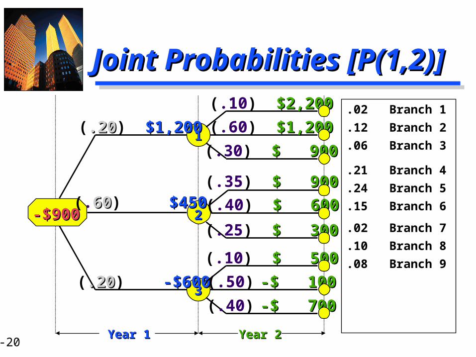
NPV for Each Cash-Flow NPV for Each Cash-Flow Stream at 5% Risk-Free RateStream at 5% Risk-Free Rate

$ 2,238.32

$ 1,331.29

$ 1,059.18

$ 344.90

$ 72.79

-$ 199.32

-$ 1,017.91

-$ 1,562.13

-$ 2,106.35

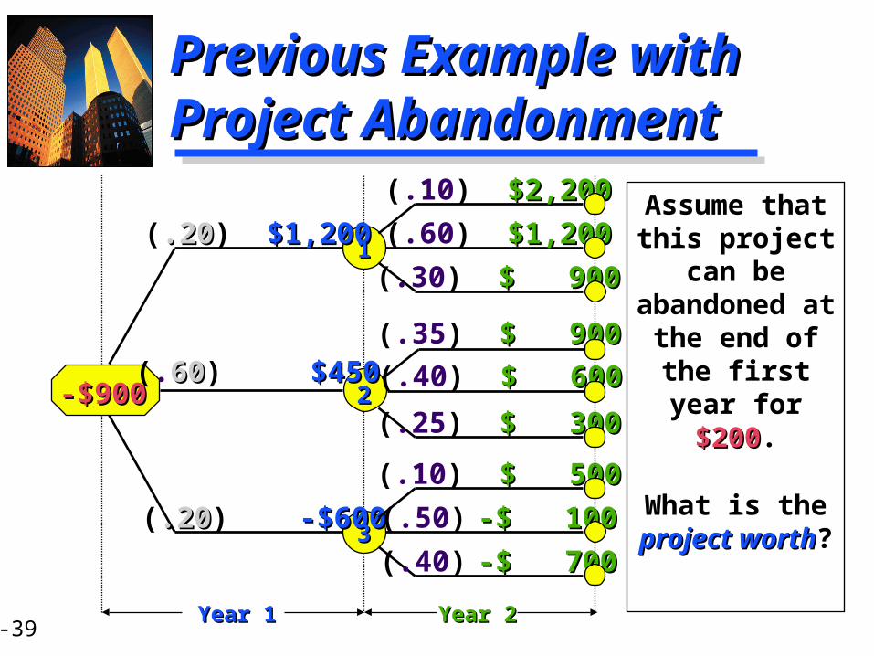
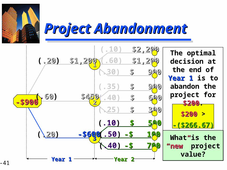
-$900-$900

(.20.20) $1,200$1,200

(.20.20) -$600-$600

(.6060) $450$450

Year 1Year 1

11

22

33

(.60) $1,200$1,200

(.30) $ 900$ 900

(.10) $2,200$2,200

(.35) $ 900$ 900

(.40) $ 600$ 600

(.25) $ 300 $ 300

(.10) $ 500$ 500

(.50) -$ 100-$ 100

(.40) -$ 700-$ 700

Year 2Year 2

14-23

NPV on the CalculatorNPV on the Calculator

Remember, we can use the cash flow registry

to solve these NPV problems quickly and

accurately!

14-24

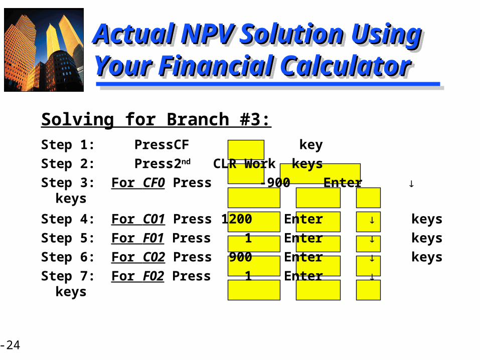
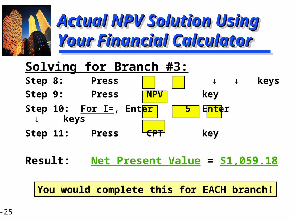
Actual NPV Solution Using Actual NPV Solution Using Your Financial CalculatorYour Financial CalculatorActual NPV Solution Using Actual NPV Solution Using Your Financial CalculatorYour Financial Calculator

Solving for Branch #3:Step 1: Press CF key

Step 2: Press 2nd CLR Work keys

Step 3: For CF0 Press -900 Enter keys

Step 4: For C01 Press 1200 Enter keys

Step 5: For F01 Press 1 Enter keys

Step 6: For C02 Press 900 Enter keys

Step 7: For F02 Press 1 Enter keys

14-25

Actual NPV Solution Using Actual NPV Solution Using Your Financial CalculatorYour Financial CalculatorActual NPV Solution Using Actual NPV Solution Using Your Financial CalculatorYour Financial Calculator

Solving for Branch #3:

Step 8: Press keys

Step 9: Press NPV key

Step 10: For I=, Enter 5 Enter keys

Step 11: Press CPT key

Result: Net Present Value = $1,059.18

You would complete this for EACH branch!

14-26

Calculating the Expected Calculating the Expected Net Present Value (Net Present Value (NPVNPV))

Branch NPV NPVii

Branch 1 $ 2,238.32Branch 2 $ 1,331.29Branch 3 $ 1,059.18Branch 4 $ 344.90Branch 5 $ 72.79Branch 6 -$ 199.32Branch 7 -$ 1,017.91Branch 8 -$ 1,562.13Branch 9 -$ 2,106.35

P(1,2) P(1,2) NPVNPVii * P(1,2) P(1,2)

.02 $ 44.77 .12 $159.75 .06 $ 63.55 .21 $ 72.43 .24 $ 17.47 .15 -$ 29.90 .02 -$ 20.36 .10 -$156.21 .08 -$168.51

Expected Net Present Value Expected Net Present Value = -$ 17.01-$ 17.01

14-27

Calculating the Variance Calculating the Variance of the Net Present Valueof the Net Present Value

NPVNPVii

$ 2,238.32 $ 1,331.29 $ 1,059.18 $ 344.90 $ 72.79-$ 199.32-$ 1,017.91-$ 1,562.13-$ 2,106.35

P(1,2) P(1,2) ((NPVNPVii - NPVNPV )2[P(1,2)P(1,2)]

.02 $ 101,730.27 .12 $ 218,149.55 .06 $ 69,491.09 .21 $ 27,505.56 .24 $ 1,935.37 .15 $ 4,985.54 .02 $ 20,036.02 .10 $ 238,739.58 .08 $ 349,227.33

Variance Variance = $1,031,800.31$1,031,800.31

14-28

Summary of the Summary of the Decision Tree AnalysisDecision Tree Analysis

The standard deviation standard deviation = SQRT ($1,031,800) = $1,015.78$1,015.78

The expected NPV expected NPV = -$ 17.01-$ 17.01

14-29

Simulation ApproachSimulation Approach

An approach that allows us to test the possible results of an

investment proposal before it is accepted. Testing is based on a model coupled with probabilistic

information.

14-30

Simulation ApproachSimulation Approach

Market analysisMarket analysis Market size, selling price, market

growth rate, and market share

Investment cost analysisInvestment cost analysis Investment required, useful life of

facilities, and residual value Operating and fixed costsOperating and fixed costs

Operating costs and fixed costs

Factors we might consider in a model:

14-31

Simulation ApproachSimulation Approach

Each variable is assigned an appropriate probability distribution. The distribution for

the selling price of baskets created by Basket Wonders might look like:

$20 $25 $30 $35 $40 $45 $50.02 .08 .22 .36 .22 .08 .02

The resulting proposal value is dependent on the distribution and interaction of EVERY variable listed on slide 14-30.

14-32

Simulation ApproachSimulation Approach

Each proposal will generate an internal rate of internal rate of returnreturn. The process of generating many, many

simulations results in a large set of internal rates of return. The distributiondistribution might look like

the following:

INTERNAL RATE OF RETURN (%)

PR

OB

AB

ILIT

YO

F O

CC

UR

RE

NC

E

14-33

Combining projects in this manner reduces the firm risk due to diversificationdiversification.

Combining projects in this manner reduces the firm risk due to diversificationdiversification.

Contribution to Total Firm Risk: Contribution to Total Firm Risk: Firm-Portfolio ApproachFirm-Portfolio ApproachContribution to Total Firm Risk: Contribution to Total Firm Risk: Firm-Portfolio ApproachFirm-Portfolio Approach

CA

SH

FL

OW

TIME TIMETIME

Proposal AProposal A Proposal BProposal BCombination of Combination of

Proposals Proposals AA andand BB

14-34

NPVP = ( NPVj )

NPVP is the expected portfolio NPV,

NPVj is the expected NPV of the jth NPV that the firm undertakes,

m is the total number of projects in the firm portfolio.

NPVP = ( NPVj )

NPVP is the expected portfolio NPV,

NPVj is the expected NPV of the jth NPV that the firm undertakes,

m is the total number of projects in the firm portfolio.

Determining the Expected Determining the Expected NPV for a Portfolio of ProjectsNPV for a Portfolio of ProjectsDetermining the Expected Determining the Expected NPV for a Portfolio of ProjectsNPV for a Portfolio of Projects

m

j=1

14-35

PP = jk

jk is the covariance between possible

NPVs for projects j and k

jk = j k rrjk .

j is the standard deviation of project j,

k is the standard deviation of project k,

rjk is the correlation coefficient between projects j and k.

PP = jk

jk is the covariance between possible

NPVs for projects j and k

jk = j k rrjk .

j is the standard deviation of project j,

k is the standard deviation of project k,

rjk is the correlation coefficient between projects j and k.

Determining Portfolio Determining Portfolio Standard DeviationStandard DeviationDetermining Portfolio Determining Portfolio Standard DeviationStandard Deviation

m

j=1

m

k=1

14-36

E: Existing ProjectsE: Existing Projects

8 Combinations

EE EE + 1 EE + 1 + 2 EE + 2 EE + 1 + 3EE + 3 EE + 2 + 3

EE + 1 + 2 + 3

AA, BB, and CC are dominatingdominating combinations from the eight possible.

Combinations of Combinations of Risky InvestmentsRisky Investments

A

B

C

E

Standard Deviation

Exp

ecte

d V

alu

e o

f N

PV

14-37

Managerial (Real) OptionsManagerial (Real) Options

Management flexibility to make future decisions that affect a

project’s expected cash flows, life, or future acceptance.

Project Worth = NPV + Option(s) Value

14-38

Managerial (Real) OptionsManagerial (Real) Options

Expand (or contract)Expand (or contract)

Allows the firm to expand (contract) production if conditions become favorable (unfavorable).

AbandonAbandon

Allows the project to be terminated early.

PostponePostpone

Allows the firm to delay undertaking a project (reduces uncertainty via new information).

14-39

Previous Example with Previous Example with Project AbandonmentProject Abandonment

Assume that this project

can be abandoned at the end of the first year for

$200$200.

What is the project project worthworth?

-$900-$900

(.20.20) $1,200$1,200

(.20.20) -$600-$600

(.6060) $450$450

Year 1Year 1

11

22

33

(.60) $1,200$1,200

(.30) $ 900$ 900

(.10) $2,200$2,200

(.35) $ 900$ 900

(.40) $ 600$ 600

(.25) $ 300$ 300

(.10) $ 500$ 500

(.50) -$ 100-$ 100

(.40) -$ 700-$ 700

Year 2Year 2

14-40

Project AbandonmentProject Abandonment

Node 3Node 3:

(500500/1.05)(.1)+ (-100-100/1.05)(.5)+ (-700-700/1.05)(.4)=

($476.19)(.1)+ -($ 95.24)(.5)+ -($666.67)(.4)=

-($266.67)-($266.67)

-$900-$900

(.20.20) $1,200$1,200

(.20.20) -$600-$600

(.6060) $450$450

Year 1Year 1

11

22

33

(.60) $1,200$1,200

(.30) $ 900$ 900

(.10) $2,200$2,200

(.35) $ 900$ 900

(.40) $ 600$ 600

(.25) $ 300 $ 300

(.10) $ 500$ 500

(.50) -$ 100-$ 100

(.40) --$ 700$ 700

Year 2Year 2

14-41

Project AbandonmentProject Abandonment

-$900-$900

(.20.20) $1,200$1,200

(.20.20) -$600-$600

(.6060) $450$450

Year 1Year 1

11

22

33

(.60) $1,200$1,200

(.30) $ 900$ 900

(.10) $2,200$2,200

(.35) $ 900$ 900

(.40) $ 600$ 600

(.25) $ 300 $ 300

(.10) $ 500$ 500

(.50) -$ 100-$ 100

(.40) -$ 700-$ 700

Year 2Year 2

The optimal decision at the end of Year 1 Year 1 is to abandon the project for

$200$200.

$200$200 >

-($266.67)-($266.67)

What is the “new” “new” project

value?

14-42

Project AbandonmentProject Abandonment

$ 2,238.32

$ 1,331.29

$ 1,059.18

$ 344.90

$ 72.79

-$ 199.32

-$ 1,280.95

-$900-$900

(.20.20) $1,200$1,200

(.20.20) -$400*-$400*

(.6060) $450$450

Year 1Year 1

11

22

33

(.60) $1,200$1,200

(.30) $ 900$ 900

(.10) $2,200$2,200

(.35) $ 900$ 900

(.40) $ 600$ 600

(.25) $ 300$ 300

(1.0) $ 0 $ 0

Year 2Year 2

*-$600 + $200 abandonment

14-43

Summary of the Addition Summary of the Addition of the Abandonment Optionof the Abandonment Option

* For “True” Project considering abandonment option

The standard deviation*standard deviation* = SQRT (740,326) = $857.56$857.56

The expectedexpected NPV*NPV* = $$ 71.8871.88

NPV* NPV* = Original NPV + Abandonment OptionAbandonment Option

Thus,Thus, $71.88 $71.88 = -$17.01 + OptionOption

Abandonment Option Abandonment Option = $ 88.89$ 88.89