1,4 DIOXANE REMOVAL FROM GROUNDWATER … · Appendix F: Initial Carbon Capacity Estimations ... 1,4...

1,4 DIOXANE REMOVAL FROM GROUNDWATER USING POINT-OF-ENTRY WATER TREATMENT

TECHNIQUES

BY

MICHAEL A. CURRY

B.S. in Civil Engineering, University of New Hampshire, 2009

THESIS

Submitted to the University of New Hampshire in Partial Fulfillment of the Requirements for the Degree of

Master of Science

In

Civil Engineering

September 2012

ii

This Thesis has been examined and approved.

.

Thesis Director, Nancy E. Kinner

Professor of Civil/Environmental Engineering

.

Thesis Co-Director, James P. Malley, Jr.


.

M. Robin Collins


iii

DEDICATION

I wish to express my gratefulness to my parents who have shown unwavering support throughout

my academic and personal endeavors.

iv

ACKNOWLEDGEMENTS

First and foremost I would like to thank my advisor Dr. Nancy Kinner for the contagious

passion she shows not only in her work, but in her students. I am lucky to have had you

in my life as a professor, an advisor, and now a longtime friend.

I would also like to thank Dr. James Malley for taking the time to lend his expertise and

insight on this project. More than any other professor at UNH you have prepared me for

what is to come not only in my professional journey, but also in life.

Thanks to the New Hampshire Department of Environmental Services, Fred McGarry,

Lou Barinelli, Sheila Heath, and Pat Bickford for providing me the opportunity to work

with them on such an interesting project. Without your help and hard work, this project

would never have left the ground.

Finally, I would like to thank Maddy and all of the students, staff, and faculty in the

Environmental Engineering department. Your positive attitudes made it easy to come

into Gregg Hall every day.

v

Contents Page

DEDICATION ................................................................................................................................ iii

ACKNOWLEDGEMENTS ............................................................................................................ iv

LIST OF TABLES ........................................................................................................................ viii

LIST OF FIGURES ......................................................................................................................... x

ABSTRACT ................................................................................................................................... xii

Chapter 1 - INTRODUCTION ........................................................................................................ 1

Use and Occurrence of 1,4 Dioxane ............................................................................................ 1

Properties of 1,4 Dioxane ............................................................................................................ 3

Health Effects and Regulations of 1,4 Dioxane ........................................................................... 4

Research Objectives ..................................................................................................................... 6

Chapter 2 – METHODS AND MATERIALS ................................................................................. 8

Objectives .................................................................................................................................... 8

Standard Preparation .................................................................................................................... 8

Air Stripping ................................................................................................................................ 8

Initial Air Stripping Experiment ............................................................................................ 10

Detailed Air Stripping Experiment ........................................................................................ 11

Activated Carbon Adsorption .................................................................................................... 12

F200 Isotherm Studies: Initial Sorption Evaluation ............................................................... 13

F200 Isotherm Studies: Revised Sorption Evaluation ........................................................... 15

F200 Isotherm Studies: Final Sorption Evaluation ................................................................ 16

GAC Comparison Isotherm Study ......................................................................................... 17

GAC Isotherm Experiments ................................................................................................... 18

Direct UV Photolysis ................................................................................................................. 22

UV-Peroxide Oxidation ............................................................................................................. 27

Initial UV-Peroxide Experiment ............................................................................................ 28

UV-Peroxide Experiment for Scavenging Effects ................................................................. 29

Analytical Methods .................................................................................................................... 30

Chapter 3 – RESULTS AND DISCUSSION ................................................................................ 31

Air Stripping .............................................................................................................................. 31

Preliminary Air Stripping Test ............................................................................................... 31

Air Stripping Test Using Typical POE A:W Ratios .............................................................. 32

Activated Carbon Adsorption .................................................................................................... 34

vi

F200 Isotherm Study .............................................................................................................. 34

GAC Comparison Isotherm Study ......................................................................................... 37

GAC Isotherm Experiments ................................................................................................... 39

UV Direct Photolysis ................................................................................................................. 45

UV-Peroxide Oxidation ............................................................................................................. 51

UV-Peroxide Experiment for Scavenging Effects ................................................................. 53

Chapter 5 – APPLICATIONS FOR RESIDENTIAL TREATMENT ........................................... 56

Air Stripping .......................................................................................................................... 56

GAC Adsorption .................................................................................................................... 57

UV Direct Photolysis ............................................................................................................. 58

UV-Peroxide .......................................................................................................................... 59

Chapter 6 – CONCLUSIONS ........................................................................................................ 60

Chapter 7 –Recommendations ....................................................................................................... 62

REFERENCES .............................................................................................................................. 63

Public Health Effects ............................................................................................................. 67

Air Stripping .......................................................................................................................... 69

Activated Carbon Adsorption ................................................................................................ 71

Bioremediation ....................................................................................................................... 72

Advanced Oxidation Processes .............................................................................................. 76

Appendix A: Literature Review ................................................................................................................... 67

Appendix B: F200 Isotherm Studies-Initial Sorption Evaluation Data ......................................................... 80

Appendix C: F200 Isotherm Studies-Revised Sorption Evaluation Data ...................................................... 81

Appendix D: F200 Isotherm Studies: Final Sorption Evaluation Data .......................................................... 82

Appendix E: GAC Comparison Isotherm Study Data ................................................................................... 83

Appendix F: Initial Carbon Capacity Estimations ......................................................................................... 84

Appendix G: GAC Comparison Graphs for Dioxane Sorption ..................................................................... 85

Appendix H: Carbon Dosage Requirements Calculations ............................................................................. 86

Appendix I: GAC Isotherm Experimental Data ............................................................................................ 87

Appendix J: IUVA-Bolton Photosciences Spreadsheet (Low Pressure-Deep Sample) ................................. 89

Appendix K: Preliminary Air Stripping Test Data ........................................................................................ 90

vii

Appendix L: Primary Air Stripping Test Data Using Typical A:W Ratios ................................................... 91

Appendix M: Initial UV Bench Scale Study Data ......................................................................................... 92

Appendix N: UV Bench Scale Study with Additional Monitoring Data ....................................................... 93

Appendix O: UV Batch Reactor Study Data ................................................................................................. 94

Appendix P: Initial UV-Peroxide Experiment Data ...................................................................................... 95

Appendix Q: UV-Peroxide Experiment Data for Scavenging Effects ........................................................... 96

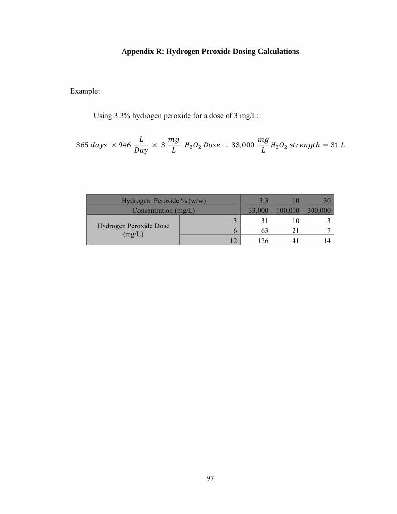
Appendix R: Hydrogen Peroxide Dosing Calculations ................................................................................. 97

Appendix S: Laboratory Percent Recovery Correction Calculation .............................................................. 99

viii

LIST OF TABLES

Table Page

Table 1: Occurrence of 1,4 Dioxane in Cleaning Finished Products ............................................................... 2

Table 2: 1,4 Dioxane Properties ...................................................................................................................... 4

Table 3: Regulatory Guidelines for 1,4 Dioxane in Water .............................................................................. 5

Table 4: Preliminary Sampling Regime for Initial Air Stripping Experiment ............................................... 11

Table 5: Sampling Regime for Detailed Air Stripping Experiment .............................................................. 11

Table 6: Activated Carbon Samples for Adsorption Studies ......................................................................... 12

Table 7: 1,4 Dioxane Standard Concentrations (C0) After 24 Hour Storage ................................................ 14

Table 8: 1,4 Dioxane Standard Concentrations for Revised Sorption Evaluation ......................................... 15

Table 9: 1,4 Dioxane Standard Concentrations for Final Sorption Evaluation ............................................. 16

Table 10: Estimated GAC Capacities ............................................................................................................ 18

Table 11: Carbon Dosage Requirements for F200 ........................................................................................ 19

Table 12: GAC Type for Comparison Study ................................................................................................. 37

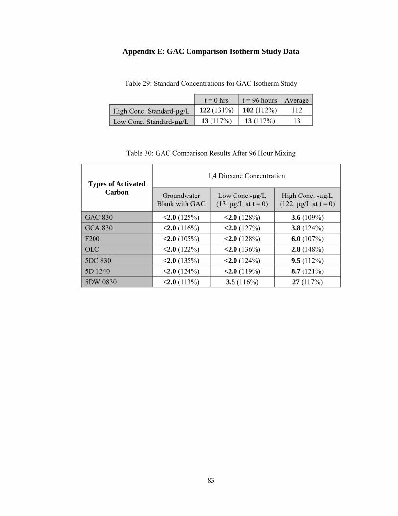
Table 13: Dioxane Concentrations in Controls Lacking GAC ...................................................................... 38

Table 14: Low and High Concentration for 1,4 Dioxane Removal Results .................................................. 38

Table 15: Initial GAC Capacities for Dioxane .............................................................................................. 39

Table 16: Freundlich Isotherm Constants for Three GAC Types .................................................................. 40

Table 17: GAC Comparison for POE Unit .................................................................................................... 44

Table 18: Drinking Water Cost ..................................................................................................................... 45

Table 19: Annual Hydrogen Peroxide Use in Liters ..................................................................................... 55

Table 20: Minimum Risk Levels for Humans as a Result of Exposure to 1,4 Dioxane (Adapted from

ATSDR) ............................................................................................................................................... 69

Table 21: Advanced Oxidation Processes for 1,4 Dioxane Removal In Water ............................................. 76

Table 22: Advanced Oxidation Processes for 1,4 Dioxane Treatment .......................................................... 77

Table 23: F200 Initial Sorption Concentration Results ................................................................................. 80

Table 24: Mass of F200 for Initial Sorption .................................................................................................. 80

ix

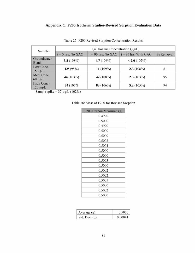
Table 25: F200 Revised Sorption Concentration Results .............................................................................. 81

Table 26: Mass of F200 for Revised Sorption ............................................................................................... 81

Table 27: F200 Final Sorption Concentration Results .................................................................................. 82

Table 28: Mass of F200 for Final Sorption ................................................................................................... 82

Table 29: Standard Concentrations for GAC Isotherm Study ....................................................................... 83

Table 30: GAC Comparison Results After 96 Hour Mixing ......................................................................... 83

Table 31: Dioxane Concentrations for Initial GAC Comparison Study ........................................................ 84

Table 32: F200 Carbon Dose Requirements .................................................................................................. 86

Table 33: OLC Carbon Dose Requirements .................................................................................................. 86

Table 34: GCA 830 Carbon Dose Requirements .......................................................................................... 86

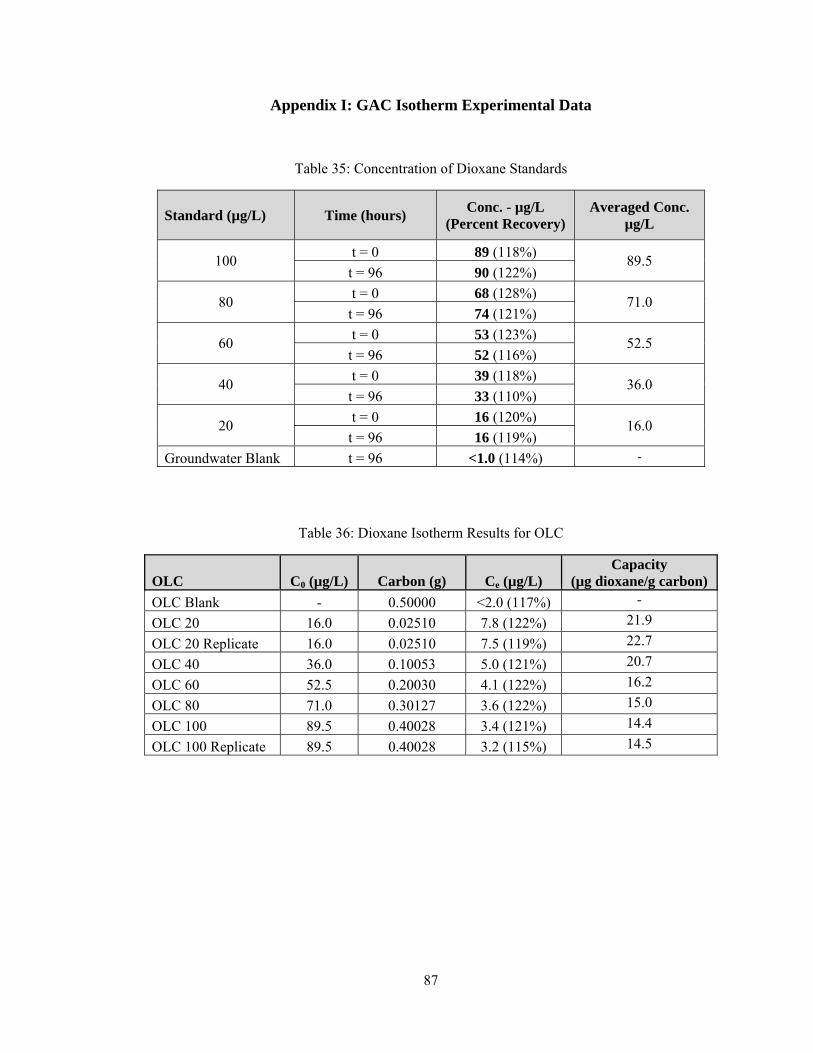
Table 35: Concentration of Dioxane Standards ............................................................................................. 87

Table 36: Dioxane Isotherm Results for OLC ............................................................................................... 87

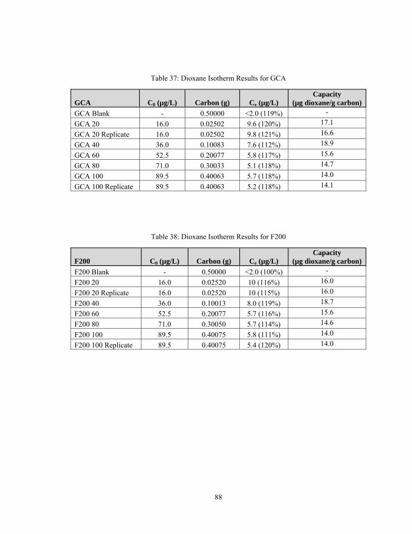
Table 37: Dioxane Isotherm Results for GCA .............................................................................................. 88

Table 38: Dioxane Isotherm Results for F200 ............................................................................................... 88

Table 39: Preliminary Air Stripping Results ................................................................................................. 90

Table 40: Air:Water Ratios for 150 mL Sample at 500 sccm ....................................................................... 90

Table 41: Primary Air Stripping Results at Typical A:W Ratios .................................................................. 91

Table 42: Air:Water Ratios for 150 mL Sample at 100 sccm ....................................................................... 91

Table 43: Initial UV Bench Scale Results (Percent Recovery) ..................................................................... 92

Table 44: UV Bench Scale Study Results with Additional Monitoring ........................................................ 93

Table 45: pH and Temperature Data for UV Bench Scale Study with Additional Monitoring .................... 93

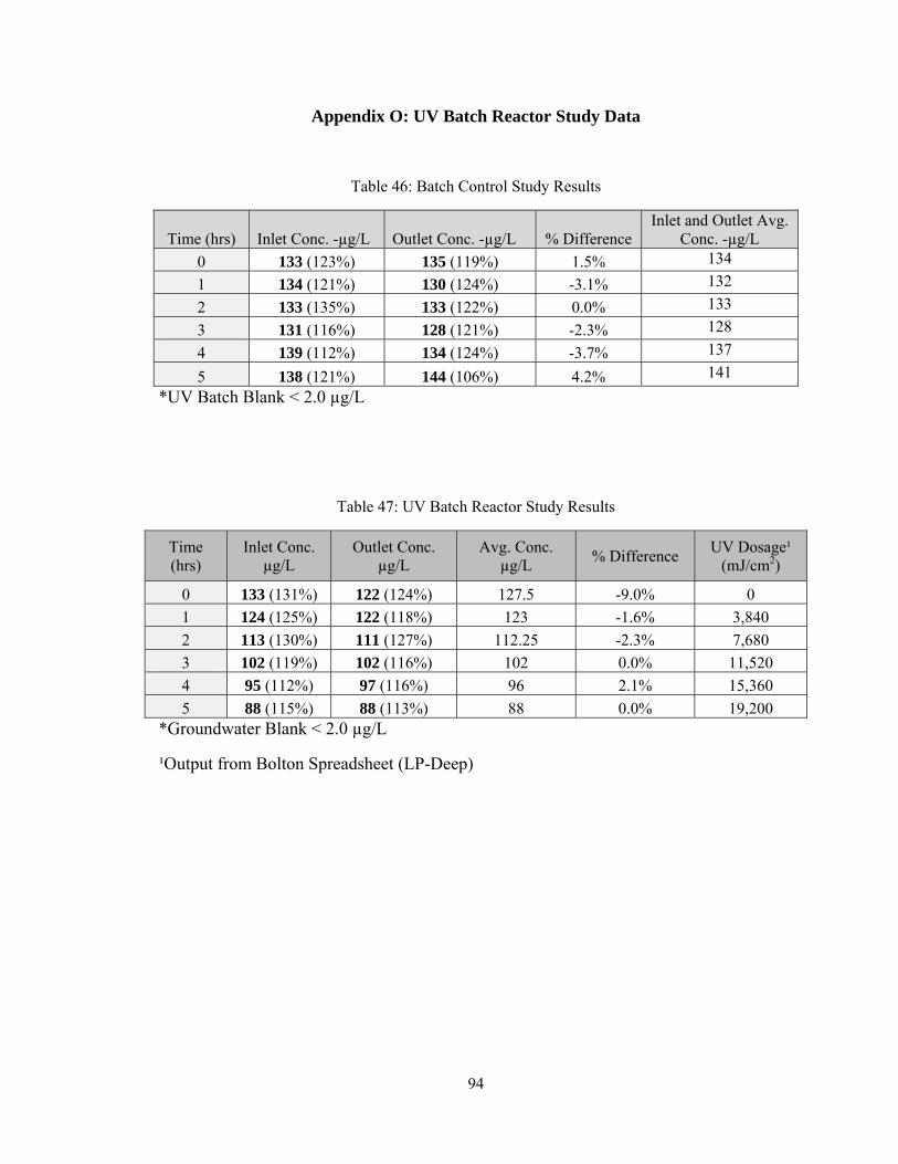
Table 46: Batch Control Study Results ......................................................................................................... 94

Table 47: UV Batch Reactor Study Results .................................................................................................. 94

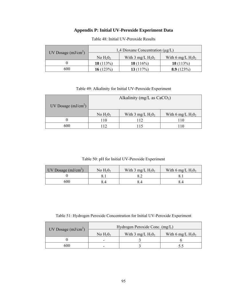
Table 48: Initial UV-Peroxide Results .......................................................................................................... 95

Table 49: Alkalinity for Initial UV-Peroxide Experiment ............................................................................. 95

Table 50: pH for Initial UV-Peroxide Experiment ........................................................................................ 95

Table 51: Hydrogen Peroxide Concentration for Initial UV-Peroxide Experiment ...................................... 95

Table 52: UV-Peroxide Results for Scavenging Effects (Percent Recovery) ................................................ 96

x

Table 53: Alkalinity Results for UV-Peroxide Experiments for Scavenging Effects .................................... 96

Table 54: pH Results for UV-Peroxide Experiment for Scavenging Effects ................................................ 96

Table 55: Hydrogen Peroxide Results for UV-Peroxide Experiment for Scavenging Effects ...................... 96

LIST OF FIGURES

Figure Page

Figure 1: 1,4 Dioxane Structure ...................................................................................................................... 1

Figure 2: Ethylene Oxide Dimerization........................................................................................................... 2

Figure 3: Schematic Representation of Gas Transfer Theory .......................................................................... 9

Figure 4: Air Stripping Experimental Setup .................................................................................................. 10

Figure 5: End-Over-End Rotary Mixer ......................................................................................................... 15

Figure 6: Collimated Beam Apparatus .......................................................................................................... 22

Figure 7: UV Batch Scale Laboratory Setup ................................................................................................. 25

Figure 8: Preliminary Air Stripping Test ....................................................................................................... 32

Figure 9: Air Stripping Test Using Typical POE A:W Ratios ...................................................................... 33

Figure 10: F200 Isotherm Study: Final Sorption Evaluation ......................................................................... 36

Figure 11: Freundlich Isotherm for OLC ...................................................................................................... 41

Figure 12: Freundlich Isotherm GCA 830 ..................................................................................................... 42

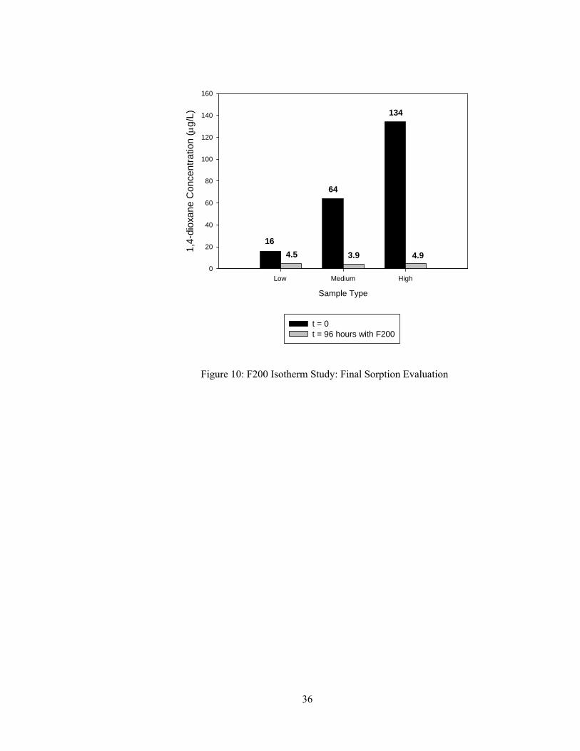
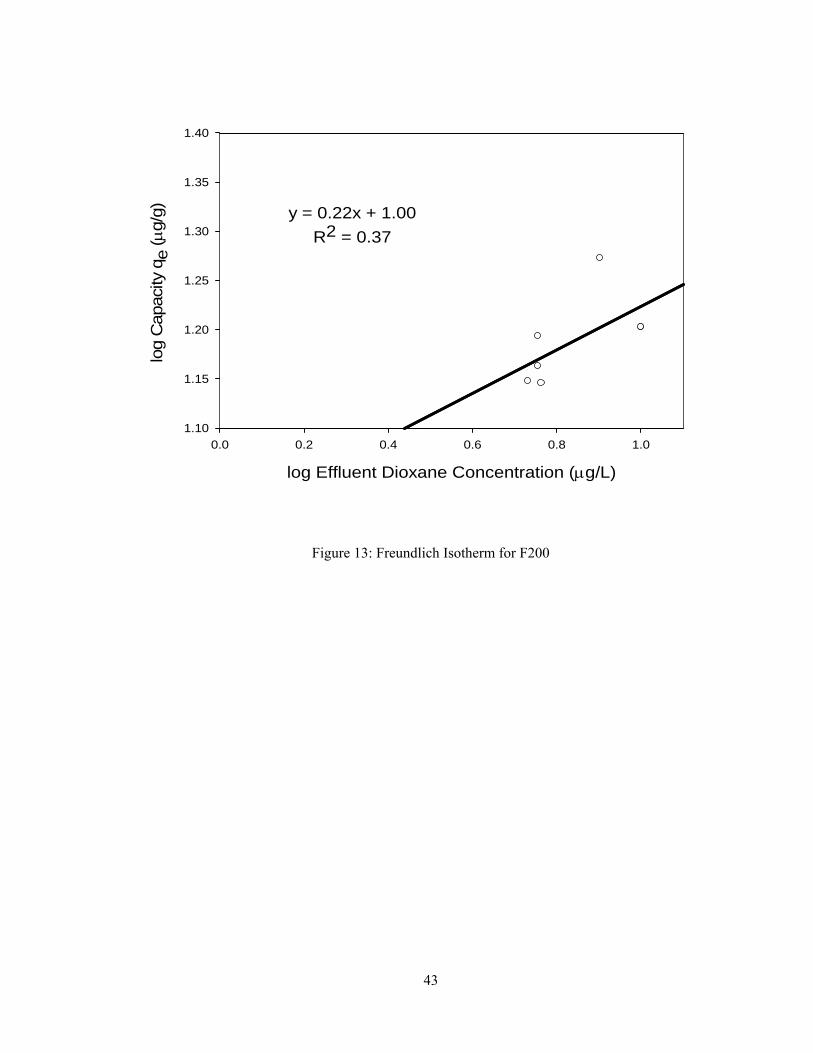
Figure 13: Freundlich Isotherm for F200 ...................................................................................................... 43

Figure 14: Initial UV Bench Scale Experiment ............................................................................................. 47

Figure 15: UV Bench Scale with Additional Monitoring .............................................................................. 48

Figure 16: UV Batch Reactor Study with SPV-8 UV Unit ........................................................................... 50

Figure 17: Initial UV-Peroxide Experiment .................................................................................................. 52

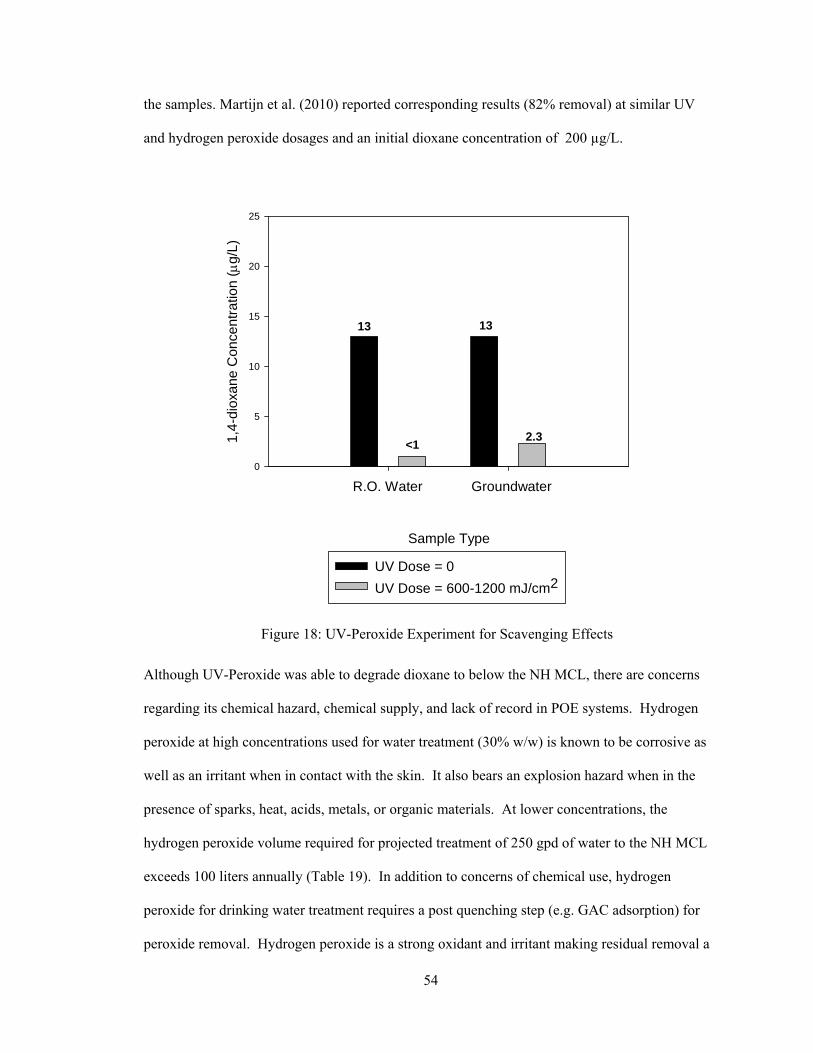
Figure 18: UV-Peroxide Experiment for Scavenging Effects ....................................................................... 54

Figure 19: Available1,4 Dioxane Health Effect Studies (ATSDR, 2007) ..................................................... 68

Figure 20: 1,4-Dioxane Model ...................................................................................................................... 70

Figure 21: Tetrahydrofuran ........................................................................................................................... 73

xi

Figure 22: High Initial Concentration GAC Comparison .............................................................................. 85

Figure 23: Low Initial Concentration GAC Comparison .............................................................................. 85

Figure 24: Bolton Photosciences Excel Spreadsheet ..................................................................................... 89

xii

ABSTRACT

1,4 DIOXANE REMOVAL FROM GROUNDWATER USING POINT-OF-ENTRY WATER TREATMENT TECHNIQUES

by

Michael A. Curry

University of New Hampshire, September, 2012

This feasibility study investigated the removal of an emerging organic contaminant, 1,4

dioxane, from groundwater using point-of-entry (POE) treatment techniques in response to its

discovery in some small New Hampshire groundwater-based private drinking water systems. The

New Hampshire Department of Environmental Services (NHDES) is evaluating future treatment

options for dioxane contamination of these small, groundwater-based private systems. Treatment

technologies assessed for dioxane removal included: air stripping, carbon adsorption, direct UV

photolysis, and UV-peroxide (H2O2) oxidation. Criteria used to assess the suitability of these

technologies for POE application included: dioxane removal efficiency, capital and operations

and maintenance (O & M) cost, ease of use, and safety. Initial tests indicated that air stripping

and direct photolysis were not feasible treatment options for a maximum contaminant level

(MCL) of 3 µg/L dioxane. Carbon adsorption and UV-Peroxide oxidation were both found to

treat dioxane to ≤ 3 µg/L (96% and 82% removal, respectively). This study determined that

carbon adsorption using a coconut-based carbon is the most feasible dioxane treatment option for

a POE system based on cost evaluations and treatment experience.

1

Chapter 1 - INTRODUCTION

Use and Occurrence of 1,4 Dioxane

1,4 dioxane, hereafter refereed to simply as “dioxane” (Figure 1), is a synthetic industrial

chemical which found its key role in the past as a stabilizer for chlorinated solvents, particularly

of 1,1,1 trichloroethane (TCA, methyl chloroform). Prior to 1957, TCA was not commonly used

because a good stabilizer was not available. Then, the United States (U.S.) patent office received

its first request to use dioxane as a stabilizer for TCA (Dow, 1954). The development of this

dioxane patent formula helped TCA earn widespread acceptance within the degreasing industry

(Doherty, 2000). Used in the electronics, metal finishing and fabric cleaning industries, dioxane

reduces the degradation of important properties of solvents (Mohr, 2001). With the 1990

enactment of the Montreal Protocol, the use of TCA has been significantly reduced because of its

ozone depleting properties. TCA production was eventually eliminated as of January 1996,

thereby decreasing this direct use of dioxane (USEPA, 2010). However, dioxane is resistant to

degradation, so it continues to be present in the environment.

Figure 1: 1,4 Dioxane Structure

O

O

H2C

H2C CH2

CH2

2

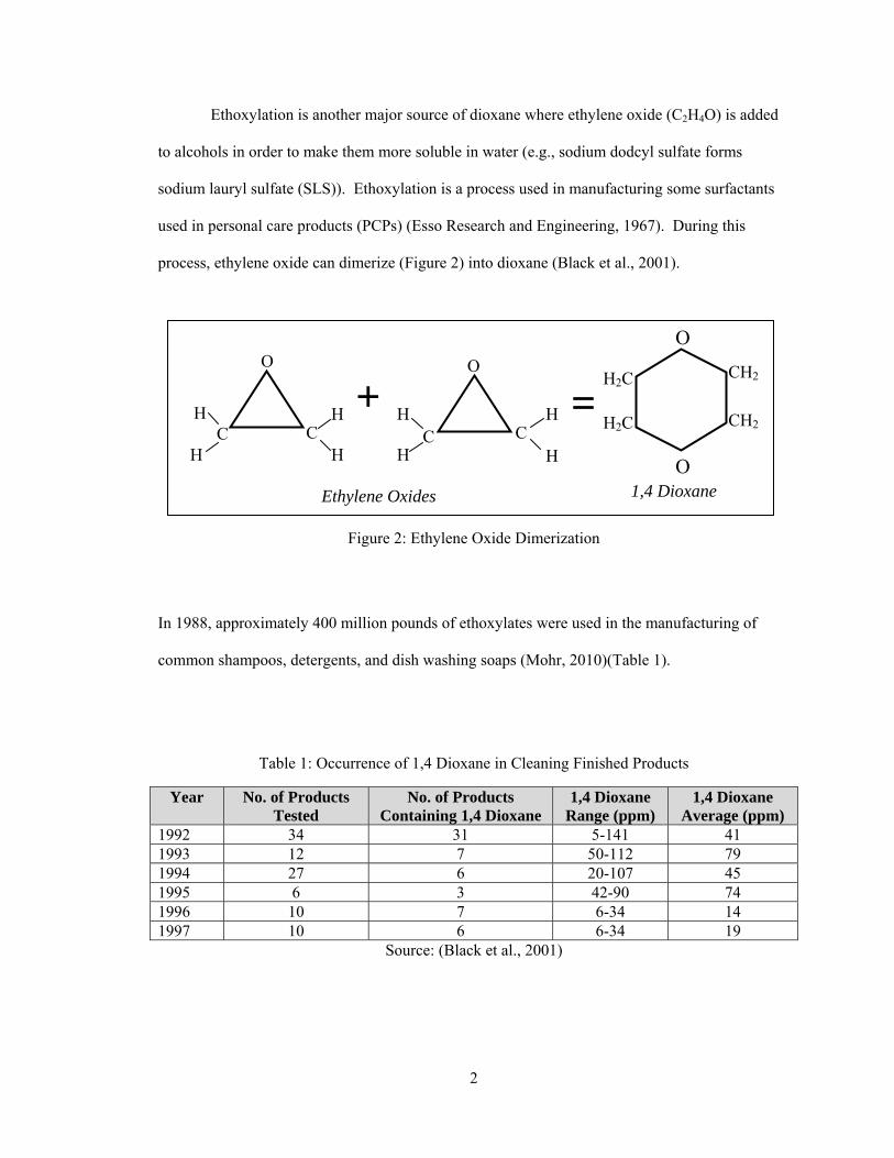
Ethoxylation is another major source of dioxane where ethylene oxide (C2H4O) is added

to alcohols in order to make them more soluble in water (e.g., sodium dodcyl sulfate forms

sodium lauryl sulfate (SLS)). Ethoxylation is a process used in manufacturing some surfactants

used in personal care products (PCPs) (Esso Research and Engineering, 1967). During this

process, ethylene oxide can dimerize (Figure 2) into dioxane (Black et al., 2001).

Figure 2: Ethylene Oxide Dimerization

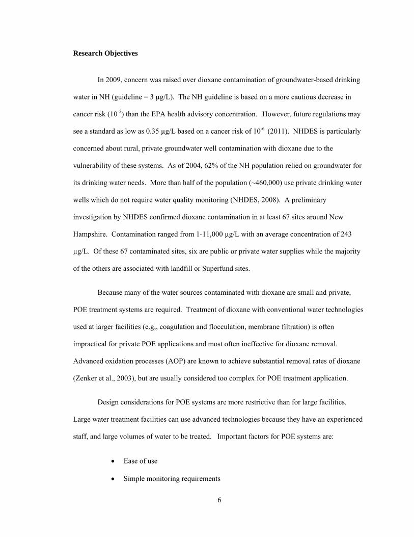
In 1988, approximately 400 million pounds of ethoxylates were used in the manufacturing of

common shampoos, detergents, and dish washing soaps (Mohr, 2010)(Table 1).

Table 1: Occurrence of 1,4 Dioxane in Cleaning Finished Products

Year No. of Products Tested

No. of Products Containing 1,4 Dioxane

1,4 Dioxane Range (ppm)

1,4 Dioxane Average (ppm)

1992 34 31 5-141 41 1993 12 7 50-112 79 1994 27 6 20-107 45 1995 6 3 42-90 74 1996 10 7 6-34 14 1997 10 6 6-34 19

Source: (Black et al., 2001)

H2C C C

O

C C

O

H

H

H

H

H

H

H

H

O

O

=+

Ethylene Oxides 1,4 Dioxane

H2C CH2

CH2

3

Along with its association with solvents and surfactants, dioxane has also been an ingredient in

the production of cellulose acetate membranes, liquid scintillation cocktails, tissue preservatives,

printing inks, paint production, adhesives, and is found in aircraft deicing fluids (Mohr, 2010).

Occurrence of dioxane in groundwater has been reported throughout the U.S. and in

countries such as Canada. In Japan, dioxane was found in 87% of a survey of surface and

groundwater samples at levels up to 95 µg/L (Abe, 1998). In December 2010, the New

Hampshire Department of Environmental Services (NHDES) found 67 locations, including

landfill and Superfund sites, at which dioxane was detected in groundwater at an average of 243

µg/L. A majority of the sites where dioxane is found are linked to industrial areas or hazardous

waste landfills. There is concern that dioxane impurities in PCPs will not be degraded in

municipal wastewater treatment facilities, subsequently contaminating natural waters.

Contamination of natural waters may lead to future problems for drinking water facilities that use

these sources. Current conventional water treatment practices (e.g., sedimentation, filtration,

biological treatment) have proven to be relatively ineffective at removing dioxane from source

water (Mohr T. K., 2010). Dioxane is also linked to groundwater impacted by waste sites where

chemical solvents (e.g., TCA) were disposed. Many NH groundwater aquifers which are

contaminated serve as potable water supplies for rural areas, where surface water sources are not

available. In these cases, point-of-entry (POE) treatment systems to remove dioxane for private

residences and other small users may be required to meet NH drinking water recommendations

(MCL1,4 Dioxane = 3 µg/L).

Properties of 1,4 Dioxane

Once released into the environment, the physical and chemical properties (Table 2) of

dioxane make it not only persistent, but difficult to treat with a POE system. Dioxane, a

4

heterocyclic ether, is resistant to biodegradation without tetrahydrofuran (THF) present as a co-

metabolite (Shangraw & Plaehn, 2006);(Zenker, 2004);(Parales et al., 1994). Its low Henry’s

Law Constant (KH) indicates it will not readily volatilize out of water. Additionally, the

unfavorable octanol-water partition coefficient (Kow) and organic carbon partition coefficient

(Koc) imply that dioxane is hydrophilic and will not adsorb to sediment, but will transport well in

groundwater. As a result, dioxane is moderately resistant to traditional treatment methods (e.g.,

air stripping, activated carbon adsorption) for the volatile organic carbons (VOCs) with which it

often co-exists (Zenker et al., 2003). Consequently, it remains a contaminant of concern (COC),

even at sites where chlorinated solvents such as TCA have been remediated.

Table 2: 1,4 Dioxane Properties

Property 1,4 Dioxane Source

Boiling Point (°C at 760 mm Hg) 101.32 (Riddick et al., 1986) Density (g/mL at 20°) 1.0336 (Riddick et al., 1986) Water Solubility (mg/L at 20°C) Miscible (Riddick et al., 1986) Octanol-Water Partition Coefficient log(Kow) -0.27 (Howard, 1990) Sorption Partition Coefficient log(Koc) 1.23 (Lyman & Rosenblatt, 1982) Henry’s Law Constant ( KH dimensionless) 1.96 × 10-4 (Howard, 1990) Maximum Rate of Microbial Utilization (kc mg of dioxane/mg total suspended solids per day)

0.45 ± 0.03 (Zenker et al., 2004)

Health Effects and Regulations of 1,4 Dioxane

Concern about dioxane contamination in groundwater has steadily increased in recent

years, due in part to advances in analytical techniques that now allow detection at low

concentrations. Human exposure pathways include inhalation of contaminated air, dermal

contact with contaminated products (e.g., shampoos, detergents), and ingestion of contaminated

water (ATSDR, 2007).

5

Citing toxicology studies, the USEPA (2009) listed dioxane as a probable human

carcinogen. The National Cancer Institute (NCI, 1978) conducted a study on the toxicity of

dioxane ingested by rats and mice and found that it had significant carcinogenic effects. More

recent studies with rats and mice show an increase in cancer occurrence, particularly of the nasal

cavity and liver when exposed to drinking water spiked with dioxane (Kano et al., 2009).

USEPA (2011) established a health advisory concentration of 35 µg/L in drinking water

based on a 10-4 increased cancer risk. Currently, no federal drinking water standards or maximum

contaminant levels (MCL) exist for dioxane, leaving regulation to individual states. Only

Colorado has adopted a water quality standard (6.1 µg/L). However, many other states are

adopting regulatory guidelines, action levels, and remediation targets (Table 3).

Table 3: Regulatory Guidelines for 1,4 Dioxane in Water

State Type of Guideline Concentration (µg/L) California Advisory Level 3 Colorado Drinking Water Standard 3.2 Connecticut Comparison Value for Risk Assessments 20 Maine Maximum Exposure Guideline 32 Massachusetts Guideline 3 New Hampshire Proposed Risk-Based Remediation Value 3 New York Dept. of Health Drinking Water Standard 600 South Carolina Drinking Water Health Advisory 70

Source: (Mohr, 2010)

6

Research Objectives

In 2009, concern was raised over dioxane contamination of groundwater-based drinking

water in NH (guideline = 3 µg/L). The NH guideline is based on a more cautious decrease in

cancer risk (10-5) than the EPA health advisory concentration. However, future regulations may

see a standard as low as 0.35 µg/L based on a cancer risk of 10-6 (2011). NHDES is particularly

concerned about rural, private groundwater well contamination with dioxane due to the

vulnerability of these systems. As of 2004, 62% of the NH population relied on groundwater for

its drinking water needs. More than half of the population (~460,000) use private drinking water

wells which do not require water quality monitoring (NHDES, 2008). A preliminary

investigation by NHDES confirmed dioxane contamination in at least 67 sites around New

Hampshire. Contamination ranged from 1-11,000 µg/L with an average concentration of 243

µg/L. Of these 67 contaminated sites, six are public or private water supplies while the majority

of the others are associated with landfill or Superfund sites.

Because many of the water sources contaminated with dioxane are small and private,

POE treatment systems are required. Treatment of dioxane with conventional water technologies

used at larger facilities (e.g,, coagulation and flocculation, membrane filtration) is often

impractical for private POE applications and most often ineffective for dioxane removal.

Advanced oxidation processes (AOP) are known to achieve substantial removal rates of dioxane

(Zenker et al., 2003), but are usually considered too complex for POE treatment application.

Design considerations for POE systems are more restrictive than for large facilities.

Large water treatment facilities can use advanced technologies because they have an experienced

staff, and large volumes of water to be treated. Important factors for POE systems are:

Ease of use

Simple monitoring requirements

7

Minimal and relatively non-hazardous chemical requirements

Low capital and operation and maintenance (O & M) costs

Minimal energy consumption

Small space requirements

Minimal noise and odor production

The objective of my research, funded by the NHDES and the University of New

Hampshire (UNH) Environmental Research Group (ERG), was to evaluate possible POE

treatment technologies to remove dioxane from private groundwater systems. Technologies

assessed included: air stripping, carbon adsorption, direct UV photolysis, and UV-Peroxide

(H2O2) advanced oxidation. Criteria used to assess the suitability of these technologies for POE

application included: dioxane removal efficiency, capital and O & M cost, ease of use, and safety.

8

Chapter 2 – METHODS AND MATERIALS

Objectives

The objective of my research, funded by the NHDES and the University of New

Hampshire (UNH) Environmental Research Group (ERG), was to evaluate possible POE

treatment technologies to remove dioxane from private groundwater systems. Technologies

assessed at the bench scale level included: air stripping, carbon adsorption, direct UV photolysis,

and UV-Peroxide (H2O2) oxidation. Criteria used to assess the suitability of these technologies

for POE application included: dioxane removal efficiency, capital and O & M cost, ease of use,

and safety.

Standard Preparation

The dioxane used in this research was reagent grade (99+ % extra pure) supplied by

Acros Organics (Waltham, MA). Groundwater was pumped from a pristine bedrock well located

on the northeast side of Gregg Hall at UNH (Durham, NH).

Air Stripping

Air stripping is a common desorption process for removing chlorinated VOCs (e.g, TCA)

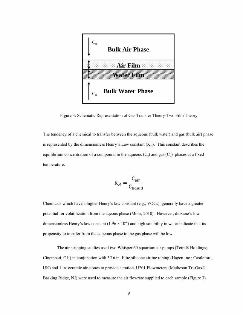
associated with dioxane in groundwater. This process (Figure 3) is governed by gas (mass)

transfer theory of the contaminant through the bulk water phase, air-water interface, and bulk air

phase (Weber, 1972).

9

Figure 3: Schematic Representation of Gas Transfer Theory-Two Film Theory

The tendency of a chemical to transfer between the aqueous (bulk water) and gas (bulk air) phase

is represented by the dimensionless Henry’s Law constant (KH). This constant describes the

equilibrium concentration of a compound in the aqueous (Ca) and gas (Cg) phases at a fixed

temperature.

KCC

Chemicals which have a higher Henry’s law constant (e.g., VOCs), generally have a greater

potential for volatilization from the aqeous phase (Mohr, 2010). However, dioxane’s low

dimensionless Henry’s law constant (1.96 × 10-4) and high solubility in water indicate that its

propensity to transfer from the aqueous phase to the gas phase will be low.

The air stripping studies used two Whisper 60 aquarium air pumps (Tetra® Holdings;

Cincinnati, OH) in conjunction with 3/16 in. Elite silicone airline tubing (Hagen Inc.; Castleford,

UK) and 1 in. ceramic air stones to provide aeration. U201 Flowmeters (Matheson Tri-Gas®;

Basking Ridge, NJ) were used to measure the air flowrate supplied to each sample (Figure 3).

Bulk Air Phase

Bulk Water Phase

Air Film

Water Film

Cg

Ca

10

Dioxane solutions were prepared within 30 minutes of the start of the experiment to minimize

volatilization losses. The temperature and pH of each sample were measured before and after the

experiment to ensure stable water chemistry and that no other reactions were occurring (e.g.,

photo-oxidation).

Initial Air Stripping Experiment

Groundwater spiked with ~120 µg/L of dioxane was aerated in 6 separate beakers over 25

hours to determine the effectiveness of air stripping (Table 4). The purpose of the initial test was

to determine if aeration could reduce the dioxane concentration in groundwater. The air flowrate

was monitored at 500 standard cm3/min (sccm) per beaker. At a fixed sample volume of 150 mL,

air to water (A:W) ratios over the experimental run ranged from 0-5,000:1. Samples were aerated

in a dark room to protect against external ultraviolet (UV) sources causing unwanted direct

photolysis of dioxane. Samples were analyzed according to USEPA Method 8260B by the

NHDES Laboratory (Concord, NH). Samples had a 14 day hold time before analysis. Reported

concentrations do not have confidence intervals because deuterated dioxane was used as a

surrogate for percent recovery.

Figure 4: Air Stripping Experimental Setup

Air stones

Whisper 60 Air pumps

U201 Flowmeter

11

Table 4: Preliminary Sampling Regime for Initial Air Stripping Experiment

Sample Type Sample Time (hours) 0 1 4 12 8 25

Non-Aerated with 1,4 Dioxane (Controls) Aerated with 1,4 Dioxane Groundwater Blank -Aerated

Detailed Air Stripping Experiment

The initial aeration test indicated that as much as 61% of the 104 µg/L dioxane was

removed from the groundwater by air stripping . Packed tower air strippers generally have air-to-

water ratios which range from 5-300 (Lagrega at al., 2001) as opposed to the 5000:1 ratio used in

the initial test. POE units used for radon removal (Kinner et al., 1990) used an air-to-water ratio

ranging from 119-156:1 dictated by pump parameters. Therefore, sampling times and air

flowrates were lowered to simulate ratios more commonly used in water treatment (A:W ≤

240:1). Lower A:W ratios resulted in shorter sampling times and decreased air flowrates (Table

5). Mixing rates among the samples were not quantified. However, mixing was not believed to

be a limiting factor due to the small sample volume (150 mL) and the air stone aeration area. The

concentration of dioxane spiked into the samples was reduced to ~50 µg/L, as this is a more

representative based on the results of NHDES survey of the state’s groundwater wells. The air

flowrate was sustained at 100 sccm in a dark room to protect against external ultraviolet (UV)

sources. The temperature and pH of each sample were measured before and after the experiment

to ensure stable water chemistry and that no other reactions were occurring (e.g., photo-

oxidation).

Table 5: Sampling Regime for Detailed Air Stripping Experiment

Sample Type Sample Time (hours) 0 0.5 1 2 4 6

Non-Aerated (Controls) with 1,4 Dioxane Aerated with 1,4 Dioxane Groundwater Blank -Aerated

12

Activated Carbon Adsorption

Adsorption is a mass transfer process in which compounds present in the liquid phase

(adsorbate) accumulate on a solid phase (adsorbent) and are thus removed from the liquid. In

drinking water treatment, this process has been used for the removal of taste and odor causing

compounds, organic and inorganic constituents and synthetic organic compounds (e.g., dioxane).

During adsorption, dissolved species diffuse into the porous carbon granules and are then

adsorbed (physically or chemically) onto the inside surface of the adsorbent. Granular activated

carbon (GAC) is known to have a wide range of pore sizes enabling it to accommodate different

types of adsorbates (Montgomery Watson Harza, 2005).

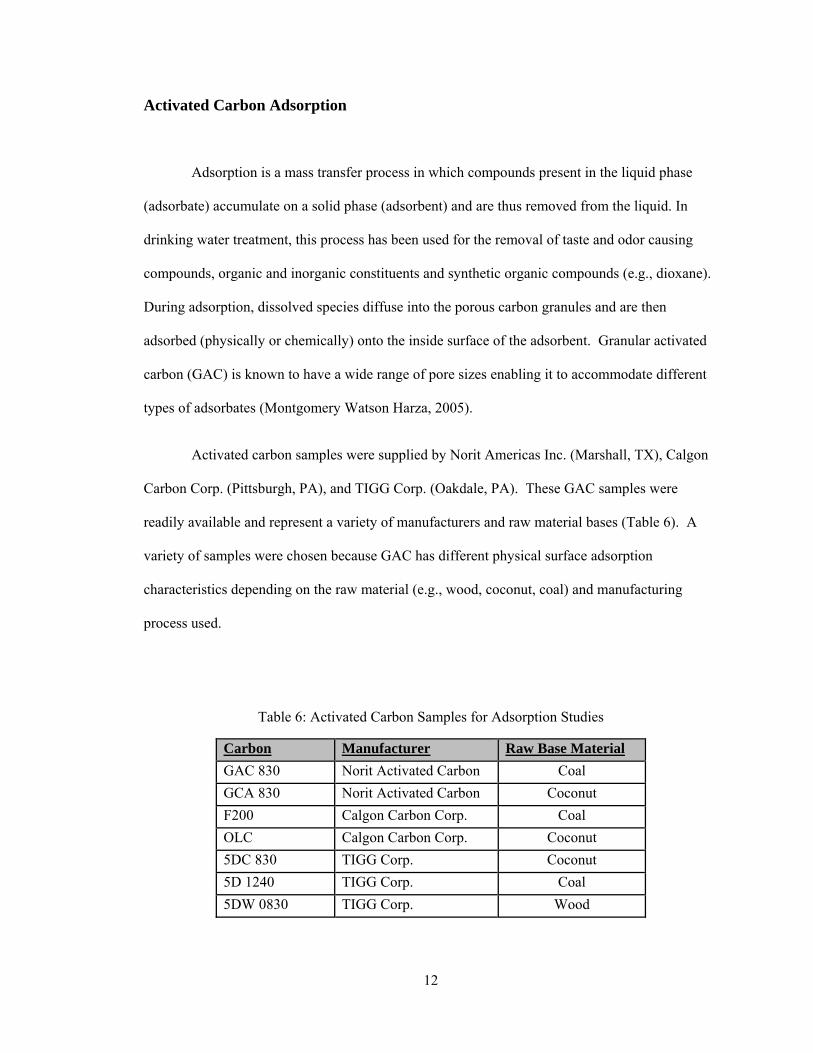
Activated carbon samples were supplied by Norit Americas Inc. (Marshall, TX), Calgon

Carbon Corp. (Pittsburgh, PA), and TIGG Corp. (Oakdale, PA). These GAC samples were

readily available and represent a variety of manufacturers and raw material bases (Table 6). A

variety of samples were chosen because GAC has different physical surface adsorption

characteristics depending on the raw material (e.g., wood, coconut, coal) and manufacturing

process used.

Table 6: Activated Carbon Samples for Adsorption Studies

Carbon Manufacturer Raw Base Material

GAC 830 Norit Activated Carbon Coal

GCA 830 Norit Activated Carbon Coconut

F200 Calgon Carbon Corp. Coal

OLC Calgon Carbon Corp. Coconut

5DC 830 TIGG Corp. Coconut

5D 1240 TIGG Corp. Coal

5DW 0830 TIGG Corp. Wood

13

The numerical portion of the carbon title represents the size of the carbon based on

standard US sieve sizes (e.g., “830” indicates granular sizes that are > 8 mesh and <30 mesh).

For all adsorption experiments, the GAC was hand crushed with a mortar and pestle in a chemical

hood. The GAC was passed through a #200 sieve, and heated in a muffle furnace to 550°C for 90

minutes to remove organic interferences.

F200 Isotherm Studies: Initial Sorption Evaluation

During this initial isotherm study, Calgon F200 carbon was used to determine the

potential capacity of dioxane sorption. The capacity of GAC for dioxane sorption is described as

microgram (µg) of dioxane sorbed per gram (g) of GAC. F200 coal-based carbon was chosen

due to its widespread use in drinking water treatment (e.g., taste and odors, chlorinated solvents).

The purpose of this study was to determine: (a) the extent to which dioxane sorption occurred

(capacity) and (b) the detectability of dioxane concentrations in the sorption experiments. A

measurable quantity of dioxane must be present in the samples at the end of an isotherm

experiment to determine the GAC adsorption capacity (mass of dioxane sorbed/mass of carbon

present). The analytical reliable detection limit (RDL) for dioxane is 2 µg/L (NHDES, 2009).

Dioxane solutions with initial targets of low, medium and high initial dioxane

concentrations (Co, Table 7) were prepared 48 hours in advance of the isotherm experiments and

refrigerated. The standard solutions were covered with aluminum foil. Results (Appendix B)

showed that these standard concentrations were lower than expected after storage.

14

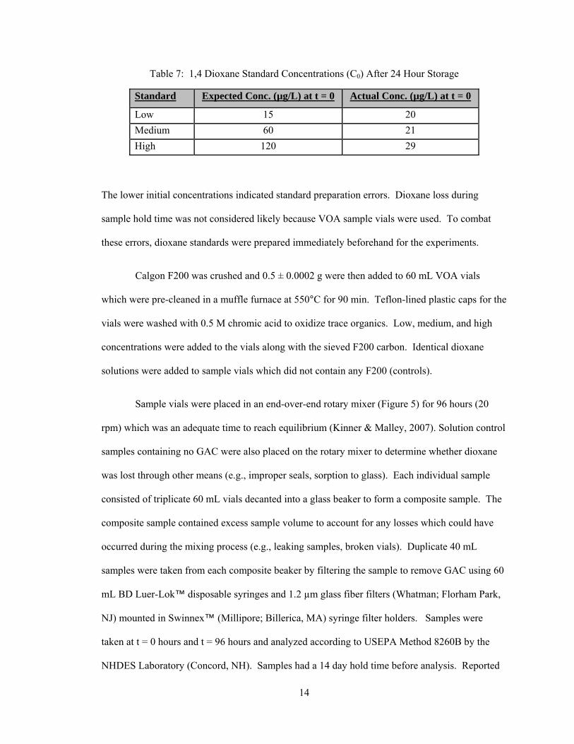
Table 7: 1,4 Dioxane Standard Concentrations (C0) After 24 Hour Storage

Standard Expected Conc. (µg/L) at t = 0 Actual Conc. (µg/L) at t = 0

Low 15 20

Medium 60 21

High 120 29

The lower initial concentrations indicated standard preparation errors. Dioxane loss during

sample hold time was not considered likely because VOA sample vials were used. To combat

these errors, dioxane standards were prepared immediately beforehand for the experiments.

Calgon F200 was crushed and 0.5 ± 0.0002 g were then added to 60 mL VOA vials

which were pre-cleaned in a muffle furnace at 550°C for 90 min. Teflon-lined plastic caps for the

vials were washed with 0.5 M chromic acid to oxidize trace organics. Low, medium, and high

concentrations were added to the vials along with the sieved F200 carbon. Identical dioxane

solutions were added to sample vials which did not contain any F200 (controls).

Sample vials were placed in an end-over-end rotary mixer (Figure 5) for 96 hours (20

rpm) which was an adequate time to reach equilibrium (Kinner & Malley, 2007). Solution control

samples containing no GAC were also placed on the rotary mixer to determine whether dioxane

was lost through other means (e.g., improper seals, sorption to glass). Each individual sample

consisted of triplicate 60 mL vials decanted into a glass beaker to form a composite sample. The

composite sample contained excess sample volume to account for any losses which could have

occurred during the mixing process (e.g., leaking samples, broken vials). Duplicate 40 mL

samples were taken from each composite beaker by filtering the sample to remove GAC using 60

mL BD Luer-Lok™ disposable syringes and 1.2 µm glass fiber filters (Whatman; Florham Park,

NJ) mounted in Swinnex™ (Millipore; Billerica, MA) syringe filter holders. Samples were

taken at t = 0 hours and t = 96 hours and analyzed according to USEPA Method 8260B by the

NHDES Laboratory (Concord, NH). Samples had a 14 day hold time before analysis. Reported

15

concentrations do not have confidence intervals because deuterated dioxane was used as a

surrogate for percent recovery (Appendix T).

Figure 5: End-Over-End Rotary Mixer

F200 Isotherm Studies: Revised Sorption Evaluation

F200 isotherm methods and materials for this study were identical to those of the initial

sorption study except for adjustments made to dioxane solution preparation. Revised from the

initial experiment, dioxane standards were prepared immediately before the test (instead of 48

hours in advance) to obtain initial concentrations (Co) closer to desired values (15-120 µg/L).

The change in procedure yielded improved results (Appendix C) for actual initial concentrations

(Table 8).

Table 8: 1,4 Dioxane Standard Concentrations for Revised Sorption Evaluation


Low 15 12

Medium 60 44

High 120 84

22 in. diameter mixer operating at 20 rpm

16

The 0.5 ± 0.0002 g of sieved F200 was added to the 60 mL VOA vials. During the experiment,

the end-over-end rotary mixer stopped for an unknown amount of time between 24-72 hours.

Consequently, these results may not be comparable to similar studies with a known contact time.

The background groundwater samples contained dioxane contamination ≤ 4.7 µg/L. Blank

groundwater contamination indicated that laboratory technique was most likely causing

contamination.

F200 Isotherm Studies: Final Sorption Evaluation

The methods and materials for this study were identical to the previous ones, except

revisions were made to the dioxane solution preparation procedure to minimize laboratory

contamination. The first adjustment was to fill and seal all blank groundwater samples before

any dioxane solutions were prepared. The second adjustment was to check the calibration of the

Eppendorf Reference© micropipetter (Hauppauge, NY) using laboratory water (reverse osmosis

water) and a laboratory scale before every solution preparation, adjusting the volume as needed.

0.5 ± 0.0006 g of sieved F200 was added to 60 mL VOA vials and mixed end-over-end for 96

hours These two adjustments yielded initial dioxane concentrations (Co) closer to desired values

and produced blank groundwater samples without detectable dioxane (RDL = 2 µg/L). Revisions

in procedure were used in all subsequent GAC studies.

Table 9: 1,4 Dioxane Standard Concentrations for Final Sorption Evaluation


Low 15 16

Medium 60 66

High 120 139

17

GAC Comparison Isotherm Study

Seven different types of GAC (Table 6) were crushed using a mortar and pestle and

sieved using an ASTM #200 sieve. 0.5 ± 0.0010 g of this GAC was added to 60 mL VOA vials

pre-cleaned in a muffle furnace at 550°C for 90 min. Teflon-lined plastic caps for the vials were

washed with chromic acid to oxidize trace organics. Dioxane solutions of low and high

concentrations were added to the vials along with the sieved GAC. Similar dioxane

concentrations were added to sample vials which did not contain any GAC to serve as controls.

Sample vials were then set in an end-over-end rotary mixer for 96 hours. Each individual

sample consisted of triplicate 60 mL vials decanted into a glass beaker to form a single composite

sample. Duplicate 40 mL samples were taken from each composite beaker by filtering the

contents using a 60 mL BD Luer-Lok™ disposable syringe and 1.2 µ glass fiber filters

(Whatman; Florham Park, NJ) mounted in a Swinnex™ (Millipore; Billerica, MA) syringe filter

holder. Samples were taken at t = 0 hours and t = 96 hours and analyzed by NHDES according

to USEPA Method 8260B. Samples had a 14 day hold time before analysis.

18

GAC Isotherm Experiments

Three GAC types with high percent dioxane removal from the initial GAC comparison

study continued through isotherm testing. These included F200 (Calgon Corp.), OLC (Calgon

Corp.), and GCA 830 (Norit Activated Carbon). The isotherm study evaluated the capacity of

each carbon for dioxane. Using results from the previous GAC experiments in this research,

capacities (qe, Table 10) were estimated for each carbon type using the Equation 1:

(eq. 1)

qe = Carbon specific capacity μ

V = Vial volume (L) M = Mass of dry carbon in vial (g) C0 = Initial dioxane concentration (

µ)

Ce = Final dioxane concentration (µ)

Table 10: Estimated GAC Capacities

Carbon Manufacturer Base Estimated Capacity (qe) µg 1,4 dioxane/ g carbon

GCA 830 Norit Activated Carbon Coconut 14.5

F200 Calgon Carbon Corp. Coal 14.2

OLC Calgon Carbon Corp. Coconut 14.6

Estimated capacities were calculated (Appendix F) using Eq.1 using initial dioxane

concentrations (C0) and carbon dosages (M) based on the initial sorption experiments. The final

dioxane concentrations (Ce) required at the end of the 96 hour mixing period could be estimated

by rearranging the equation to:

C eq.2

19

Final dioxane concentrations (Ce) of ~15 µg/L were desired, so the initial carbon dosages could

be calculated for F200 as shown in Table 11. 15 µg/L was chosen as it is significantly greater

than the RDL of 2.0 µg/L. The carbon dosage requirements for the other two GAC types are

shown in Appendix G.

Table 11: Carbon Dosage Requirements for F200

Sieved GAC was added to 60 mL VOA vials pre-cleaned in a muffle furnace at 550°C for

90 minutes. Teflon-lined plastic caps for the vials were washed with chromic acid to remove

trace organics. Dioxane solutions of 20, 40, 60, 80, and 100 µg/L were added to the vials along

with the sorted GAC. Replicate samples for the 20 and 100 µg/L samples were prepared to test

for experimental variability. Identical dioxane solutions were added to sample vials which did

not contain any GAC to serve as controls.

Sample vials were placed in an end-over-end rotary mixer for 96 hours. Each individual

sample consisted of duplicate 60 mL vials decanted into a glass beaker to form a single composite

sample. Duplicate 40 mL samples were taken from each composite beaker by filtering the

contents using 60 mL BD Luer-Lok™ disposable syringes and 1.2 µm glass fiber filters mounted

in Swinnex™ the syringe filter holders. Samples were taken at t = 0 hours and t = 96 hours and

analyzed by the NHDES according to the USEPA Method 8260B.

Where qe(µg/g) = 14.2 (Table 10)

C0 (µg/L) Mass of GAC (g) Volume of Mixing Vials (L) Ce (µg/L)

100 0.4 0.067 15.2

80 0.3 0.067 16.4

60 0.2 0.067 17.6

40 0.1 0.067 18.8

20 0.025 0.067 14.7

20

Results from the 96 hour mixing study were used to calculate capacities (qe) at each

concentration. These capacities and concentrations were applied to the Freundlich equation

which is commonly applied to powdered carbons used for water treatment (Weber, 1972):

q (Eq. 3)

qe = carbon specific capacity μ

= constant μ

1/n

= constant (unitless)

Ce = effluent dioxane concentration (µ)

Rearranging Eq. 3 indicates units for KF as ⁄

⁄. To simplify the units of KF

and in this study, they were constants. As long as the effluent dioxane concentrations were

calculated in , then the capacity (qe ) can be reported in

. Data used with the

Freundlich equation are generally fitted to the logarithmic form which yields a straight line with a

slope of and an intercept equal to log .

logq log log Eq.4

Using the logarithmic Freundlich equation and a linear regression from isotherm plots, the

Freundlich constants were calculated for each carbon type. With these constants, new Freundlich

capacities were calculated at specific initial dioxane concentrations to compare potential GAC

21

exhaustion time, effluent quality and cost of the GAC for POE application. In following the

procedure used by Kinner and Malley (2007), the calculated capacity of the carbon was not

corrected for the use of crushed carbon, also known as powdered activated carbon (PAC).

Comparison of PAC to GAC dosage based on the value of 1/n indicates that GAC capacities in

this study may be slightly underestimated.

22

Direct UV Photolysis

Ultraviolet (UV) photolysis is the process by which energy from UV light (photons) is

absorbed by molecules causing a photochemical change (degradation). This process is largely

controlled by three factors including: (a) how well the target molecule (dioxane) absorbs UV light

of a specific wavelength (molar absorption), (b) how much UV light the target molecule requires

for photochemical degradation (quantum yield), and (c) how well the water matrix transmits light

(UV absorbance). Both molar absorption (ε) and quantum yield (Ф) are chemically dependent on

molecular structure (Linden & Rosenfeldt, 2010). Research has shown that dioxane has a

relatively low molar absorptivity coefficient (ε) indicating that it is not likely to undergo

significant photochemical reactions (Martijn et al., 2010; Stefan & Bolton, 1998). The third

factor, UV absorbance (A), can be affected by various dissolved or suspended constituents in the

water matrix (e.g., natural organic matter, metals, turbidity, nitrate) (Linden & Rosenfeldt, 2010).

Methods for UV photolytic research were described and standardized by Bolton &

Linden (2003). UV direct photolysis (and UV-peroxide) experiments used a collimated beam

apparatus (Figure 6) with a low pressure high output (LPHO) mercury lamp (Ondeo Infilco

Degrémont Inc.; LPHO; Richmond; VA).

Figure 6: Collimated Beam Apparatus

Metal casing with LPHO Mercury Lamp inside

Aperture/Shutter

Sample

Irradiation Stage with Stir Plate

23

LPHO lamps emit 85% of their UV light at a wavelength of 254 nm (Linden & Rosenfeldt,

2010). Appropriate UV dose or fluence (mJ/cm2) was calculated as the product of the average

irradiance (mW/cm2) and exposure time using an Excel spreadsheet provided by Bolton

Photosciences Inc. (2004)(Appendix H). UV irradiance of the collimated beam was measured

over the exposure surface area of the sample using a radiometer (International Light

Technologies; IL1700; Peabody; MA) known to be within calibrated specifications of ± 5%

(Malley, 2011). Sample absorption coefficients were measured using a spectrophotometer

(Hitachi High Technologies Corp.; U-2000; Tokyo, Japan). The spreadsheet computed the

average irradiance ( using inputs including UV irradiance readings, sample volume (mL),

sample diameter, distance from UV lamp to top of water surface, and sample absorption

coefficient (cm-1) at 254 nm. These inputs in the IUVA-Bolton Photosciences spreadsheet

combine to help calculate the petri factor, reflection factor, water factor, and divergence factor of

the sample in order to correct the UV dose for the experimental setup and sample conditions.

Once all inputs to the IUVA-Bolton Photosciences spreadsheet are made, the user enters the

desired UV dosages and is provided with required irradiation times for a particular sample.

Initial UV Bench Scale Study

Initial UV experiments compared water samples which were irradiated with UV light

(collimated beam apparatus, Figure 6) to those samples which were not. UV irradiance readings,

sample volume (mL), sample diameter, distance from UV lamp to top of water surface, and the

sample absorption coefficient (cm-1) at 254 nm were entered into the IUVA-Bolton Photosciences

spreadsheet to determine the time required for a sample to receive a specific UV dose

(mJ/cm2)(Appendix G). The initial UV dose used was 10,000 mJ/ cm2, equivalent to an exposure

time of 25.5 hours. A high UV dose was chosen to verify if direct photolysis had the ability to

degrade dioxane.

24

A groundwater solution containing ~130 µg/L of dioxane was prepared. 150 mL of this

standard were placed into two 250 mL chromic acid (0.5 M) washed beakers with stir bars. One

sample beaker was positioned on the irradiation stage under the collimated beam apparatus, while

the other sample beaker was placed in a dark room to prevent stray UV exposure. Both beakers

were stirred for the duration of the experiment. Duplicate 40 mL samples of each were taken at t

= 0 hours and t = 25.5 hours and analyzed by NHDES using USEPA Method 8260B.

UV Bench Scale Study with Additional Monitoring

This study was designed to determine the cause of significant dioxane reductions

observed in both the irradiated and non-irradiated samples during the initial UV bench scale

study. The procedure used was the same as the initial UV bench scale study except for the

addition of two samples: (1) a beaker that was neither irradiated nor stirred, and (2) another

beaker which was sampled and sealed immediately. To further prevent stray UV exposure, a

black cloth covered the collimated beam apparatus during the experiment. Samples were also

monitored for temperature and pH changes before and after the experiment.

A groundwater solution containing ~20 µg/L of dioxane was prepared. 150 mL of this

standard were placed into four 250 mL acid-washed beakers, two of which contained stir bars.

One beaker (stirred) was positioned under the collimated beam apparatus, while the other two

beakers (only one stirred) were placed in a dark environment to avoid external UV exposure. The

fourth beaker was sampled immediately and sealed. Duplicate 40 mL samples were taken at t = 0

hours and t = 25.5 hours and analyzed according to EPA Method 8260B.

25

UV Batch Study with SPV-8 UV Reactor

Although direct photolysis bench scale studies yielded only marginal dioxane removals,

a final batch scale study was conducted using a small LPHO UV reactor. A Sterilight Platinum

SPV-8 series reactor was used with an ICE Controller (Trojan Technologies; London, ON)

capable of supplying a UV dose of 40 mJ/cm2 at a flow of ~30 Lpm (8 gpm). This reactor was

turned on 30 minutes before use to allow proper warm-up. A 18.9 liter (5 gal.) low-density

polyethylene carboy (Thermo Fisher Scientific Nalgene®; Waltham, MA) and I/P Masterflex®

Standard BDC Drive peristaltic pump (Cole-Palmer Instrument Co.; Vernon Hills, IL) were used

in the batch system (Figure 7). The pump used an Easy Load Masterflex® I/P Drive Head and

Masterflex® Tygon Long Flex Life #73 tubing. The system was constructed with PVC sampling

ports, before (inlet) and after (outlet) the UV reactor. All fittings and sealing tape used were

either Teflon or PVC.

Figure 7: UV Batch Scale Laboratory Setup

A common table salt tracer was used to find the time required for complete mixing within

the system. The UV reactor remained off during the tracer experiment. The reservoir was filled

SPV-8 UV LPHO Reactor

19 liter LDPE Carboy

#73 Tygon tubing Peristaltic Pump

ICE Controller

26

with 17.9 L of reverse osmosis water and the pump operated at ~3.8 Lpm (1 gpm). A

conductivity meter (Oakton® Instruments; Vernon Hills, IL) was lowered into the reservoir and

the conductivity (µS) recorded. A 1 L solution of R.O. water and a salt concentration of 2,000

mg/L was spiked into the reservoir and the conductivity was measured until equilibrium was

reached at 2.5 minutes. Dioxane was added in the batch scale study in the same 1 L spike

method.

The first control (no dioxane) study used 18.9 L (5 gal.) of reverse osmosis water pumped

through the system at ~3.8 Lpm. After 5 hours of exposure (UV dose = 19,200 mJ/cm2),

duplicate samples were taken from the outlet sampling point to test for dioxane. The sample had

a dioxane concentration of <2.0 µg/L (RDL). The UV reduction equivalent of this reactor is a

function of flow and UV transmittance of the water using biodosimetry with MS-2 and Bacillus

pumilus (Malley, 2011).

For the second control study, the reservoir was filled with 17.9 L of groundwater and the

pump turned on (~3.8 Lpm). A 1 L dioxane spike was slowly introduced to the top of the

reservoir to create an overall concentration of ~130 µg/L. The UV reactor remained off for this

test. Duplicate 40 mL samples were taken from the inlet and outlet ports (t = 2.5 min. and 1, 2, 3,

4, 5 hours). Changes in dioxane concentration occurred, but by other means (e.g, aeration) not be

attributed to UV direct photolysis.

For the UV irradiation study, the reservoir was filled with 17.9 L of groundwater and the

pump turned on (~3.8 Lpm). With the UV reactor on, a 1 L dioxane spike was slowly introduced

to the top of the reservoir to create an overall concentration of ~130 µg/L. Duplicate 40 mL

samples were taken from the inlet and outlet ports (t = 2.5 min. and 1, 2, 3, 4, 5 hours).

All samples were analyzed according to EPA Method 8260B by the NHDES Laboratory.

27

UV-Peroxide Oxidation

UV-peroxide oxidation is an advanced oxidation process (AOP) by which hydrogen

peroxide (~2-10 mg/L), in the presence of UV light, disassociates to form two hydroxyl radicals

(OH·).

H2O2 + UV →2 OH·

Hydroxyl radicals are some of the strongest chemical oxidants known and are effective for

destruction of many organic contaminants in water (Linden & Rosenfeldt, 2010). Similar to

direct UV photolysis, the disassociation process is limited by the quantum yield (Ф) and molar

absorption (ε) of the target molecule (hydrogen peroxide). Although hydrogen peroxide has a

high hydroxyl radical quantum yield, hydrogen peroxide is a very good absorber of UV light

(Stefan & Bolton, 1998) thereby limiting the creation of hydroxyl radicals in the UV-peroxide

process. Just as with direct photolysis, the UV absorbance (A) of the water matrix by various

dissolved or suspended constituents (e.g., natural organic matter, metals, turbidity, nitrate) can

also affect the efficiency of hydroxyl radical production (Linden & Rosenfeldt, 2010).

In addition to UV absorption limitations in the UV-peroxide process, there are also

problems associated with hydroxyl radical scavenging. Hydroxyl radicals are non-selective

oxidants and may be scavenged by carbonate species (alkalinity), natural organic matter, reduced

metal ions (e.g., Fe2+), and sulfide (Montgomery Watson Harza, 2005).

Bench scale studies for UV-Peroxide oxidation were similar to those for direct UV

photolysis (Bolton & Linden, 2003) with a few supplemental steps including the addition of

monitoring for hydrogen peroxide and alkalinity to assess hydroxyl scavenging effects. UV-

peroxide experiments used the collimated beam apparatus (Figure 5) with a low pressure high

output (LPHO) mercury lamp. The desired UV dosage (mJ/cm2) was determined using the same

28

method and spreadsheet (Bolton Photosciences, 2004) as for direct UV photolysis. Hydrogen

peroxide for this study was 3.3% w/w (Acros Organics; Waltham, MA) and measured using self-

filling reagent ampoules (CHEMetrics, Inc.; Calverton, VA). The pH of each sample was

measured with an Accumet Excel XL 50 meter kit and ATC probe (Fisher Scientific; Waltham,

MA) before and after the experiments. Alkalinity (mg/L as CaCO3) was monitored for hydroxyl

scavenging capability in each sample before and after the experiment using the HACH® Digital

Tritrator Method 8203.

Initial UV-Peroxide Experiment

The initial experiment compared water samples at hydrogen peroxide concentrations of 0,

3, and 6 mg/L irradiated at a UV dose of 600 mJ/ cm2 (1.5 hour exposure). These values were

selected based on existing water reuse facilities with UV-peroxide systems for micropollutant

destruction (Martijn et al., 2010).

A groundwater solution containing ~20 µg/L of dioxane was prepared. This study

consisted of three phases, one for each peroxide concentration. For Phase I: 150 mL of the 20

µg/L dioxane standard was added to two muffled (550°C) and cooled 250 mL beakers with stir

bars. One sample beaker was positioned under the collimated beam apparatus, while the other

beaker was placed in a darkened room to avoid external UV exposure. No hydrogen peroxide

was added to either sample. The beakers were stirred for 1.5 hours (UV dose = 600 mJ/ cm2) and

duplicate 40 mL samples taken. For Phase II: 500 mL of the standard was spiked with 3 mg/L

H202. 150 mL of this solution was then measured into two acid-washed 250 mL beakers with stir

bars. One sample beaker was positioned under the collimated beam apparatus, while the other

was placed in a darkened room to avoid external UV exposure. Both beakers were stirred for 1.5

hours and duplicate 40 mL samples taken. The beaker which contained hydrogen peroxide was

29

measured after irradiation for residual concentrations. For Phase III: this phase was identical to

Phase II, except that 6 mg/L H202 was added to the solution instead of 3 mg/L.

All samples were analyzed according to EPA Method 8260B by the NHDES Laboratory.

UV-Peroxide Experiment for Scavenging Effects

Marginal dioxane reduction results from UV-peroxide Phase II and III indicated the

possibility of hydroxyl radical scavenging by naturally occurring alkalinity. This study was

designed to: 1) determine if hydroxyl scavenging was occurring, and 2) determine if a higher dose

of UV and H202 would be more effective.

Phase I: To determine if hydroxyl scavenging was occurring, R.O. water was substituted

for groundwater due to its lack of interferences. An R.O. solution containing ~15 µg/L of

dioxane was prepared and spiked with a hydrogen peroxide to provide a dose of 3 mg/L in the

sample. 150 mL of this solution was added into a muffled 250 mL beaker with a stir bar. The

beaker was stirred and irradiated for 1.5 hours (UV dose = 600 mJ/ cm2) and duplicate 40 mL

samples taken. H202was measured for initial and residual concentrations.

For Phase 2: A groundwater solution containing ~15 µg/L of dioxane was prepared and

spiked with a hydrogen peroxide dose of 12 mg/L. 150 mL of this solution was then added to two

acid-washed 250 mL beakers with stir bars. One sample beaker was positioned under the

collimated beam apparatus, while the other beaker was placed in a closed room to avoid external

UV exposure. Both beakers were stirred for 3.2 hours (UV dose = 1200 mJ/ cm2, 2× the exposure

time and UV dose) and duplicate 40 mL samples taken. H202was measured for initial and

residual concentrations.

30

Analytical Methods

All 1,4 dioxane studies used pre-cleaned vials for sampling and were analyzed by the

NHDES according to EPA Method 8260B for volatile organic compounds by gas

chromatography/mass spectrometry (GC/MS). The preparation technique used was a heated

purge and trap for aqueous samples, EPA Method 5030. The reliable detection limit (RDL) of

dioxane for this method was 2.0 µg/L for samples received between September 9th, 2009 and

October 25th, 2010 and 1.0 µg/L for dioxane samples received after. Dioxane concentrations

were reported corrected for the percent recovery (%R) of a surrogate standard used, 1,4 dioxane-

d8, or deuterated 1,4dioxane (Appendix T). Major interferences for this method include the

presence of VOCs and large amounts of suspended solids.

The pH of samples was measured with an Accumet Excel XL 50 meter kit and ATC

probe (Fisher Scientific; Waltham, MA) following the electrometric method, Standard Method

4500B. The pH meter was calibrated weekly at minimum on a 3 point calibration curve.

Alkalinity (mg/L as CaCO3) was monitored for hydroxyl scavenging capability using the

HACH® Digital Titrator Method 8203 (Standard Method 2320B). This method has a range of

10-4000 mg/L as CaCO3.

Hydrogen peroxide measurements in the UV-peroxide study were done with self-filling

reagent ampoules using the Ferric Thiocyanate Method (Boltz & Howell, 1978). The detection

range was from 0-1 and 1-10 mg/L H202 with a MDL of 0.05 mg/L.

31

Chapter 3 – RESULTS AND DISCUSSION

This laboratory study was designed to determine the effectiveness of four potential POE

water treatment systems (e.g., air stripping, activated carbon adsorption, UV direct photolysis,

and UV-peroxide oxidation) to cost effectively remove dioxane from groundwater and meet

NHDES maximum contaminant level guidelines (NH MCL) of ≤ 3 µg/L. Important selection

factors considered for POE water treatment units include: ability to meet the NHDES MCL, ease

of use, monitoring and chemical requirements, noise and odor production, energy consumption,

footprint, and capital and O & M costs.

Air Stripping

Preliminary Air Stripping Test

The initial air stripping study was designed to investigate the unidentified dioxane losses

in direct photolysis experiments. Not initially considered viable as a treatment option, further

literature research (Appendix A) showed a 30% reduction in high dioxane concentrations (610

µg/L) was possible using high A:W ratios (Bowman, 2001). Our preliminary study compared

two groundwater samples spiked with dioxane (~100 µg/L), one aerated at 500 sccm for 25 hours

and one not. Results showed 61% and 22% reductions in the aerated and non-aerated samples,

respectively (Figure 8). The difference between the two samples (39%) indicated that air

stripping had a significant effect on the dioxane concentration. A definitive cause for the 22%

dioxane reduction in the control samples is unknown; however, likely causes include

volatilization and/or analytical variability. While these results (Appendix J) compared favorably

with dioxane reductions of 30% reported by Bowman (2001), such high dioxane removal rates

32

(61%) could be attributed to the initial high dioxane concentration (Co~100 µg/L) and the high

volume of air supplied (A:W = 5000:1) in this study.

Time (hours)

0 5 10 15 20 25 30

1,4-

Dio

xane

Con

cent

ratio

n (

g/L)

0

10

20

30

40

50

60

70

80

90

100

110

Aerated SampleNon-Aerated Sample

Figure 8: Preliminary Air Stripping Test

Air Stripping Test Using Typical POE A:W Ratios

Following the preliminary experiment, revisions were made to determine if air stripping

could be successfully applied at typical POE A:W ratios as described by Kinner et al., (1990).

They found that homeowners disliked the noise caused by the POE aeration units and would

unplug them. Therefore, experimental conditions were revised to include lower A:W ratios (1-

240:1) as well as lower influent dioxane concentrations (~30 µg/L) to better mimic a typical POE

application. Lower A:W ratios were achieved by decreasing the airflow rate and sampling time to

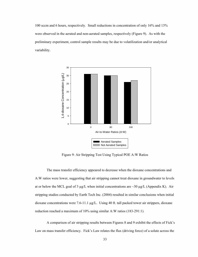
33

100 sccm and 6 hours, respectively. Small reductions in concentration of only 16% and 13%

were observed in the aerated and non-aerated samples, respectively (Figure 9). As with the

preliminary experiment, control sample results may be due to volatilization and/or analytical

variability.

Air-to-Water Ratios (A:W)

0 80 240

1,4-

diox

ane

Con

cent

ratio

n (

g/L)

0

5

10

15

20

25

30

35

Aerated SamplesNot Aerated Samples

64

16

Figure 9: Air Stripping Test Using Typical POE A:W Ratios

The mass transfer efficiency appeared to decrease when the dioxane concentrations and

A:W ratios were lower, suggesting that air stripping cannot treat dioxane in groundwater to levels

at or below the MCL goal of 3 µg/L when initial concentrations are ~30 µg/L (Appendix K). Air

stripping studies conducted by Earth Tech Inc. (2004) resulted in similar conclusions when initial

dioxane concentrations were 7.6-11.1 µg/L. Using 40 ft. tall packed tower air strippers, dioxane

reduction reached a maximum of 10% using similar A:W ratios (183-291:1).

A comparison of air stripping results between Figures 8 and 9 exhibit the effects of Fick’s

Law on mass transfer efficiency. Fick’s Law relates the flux (driving force) of a solute across the

34

air-to-water interface as a function of the concentration gradient between the phases. Because the

concentration gradients in Figure 9 were lower than that in Figure 8, the overall transfer rates

decreased. The limitations presented in Fick’s Law make air stripping difficult at low

concentration commonly associated with dioxane contamination. Steps to overcome mass transfer

limitations (e.g., increasing the mass transfer interface, increasing air flow) could potentially

result in further dioxane reduction; however, results obtained in the air stripping experiments as

well as results found in the literature indicate that air stripping is not a viable treatment option to

treat dioxane to levels required by New Hampshire.


Limited carbon isotherm data is available for dioxane from manufacturers because the

Kow suggests adsorption is not an effective treatment method. Despite this, the Beede waste oil

Superfund site (Plaistow, NH) obtains 90% dioxane reduction in their effluent using GAC filters

in place for chlorinated solvent removal. These results created interest in generating carbon

adsorption isotherms for dioxane. The purpose of the isotherm studies was to determine if

commercially available GAC could cost effectively treat dioxane to ≤ 3 µg/L.

F200 Isotherm Study

Initial isotherm studies used Calgon’s F200 coal based carbon (GAC) because of

established track record for many contaminants as well as its common use in NH POE systems

(e.g., MtBE). F200 is used in POE units installed in NH homes for treatment of MTBE

contamination in drinking water (Kinner and Malley, 2007).

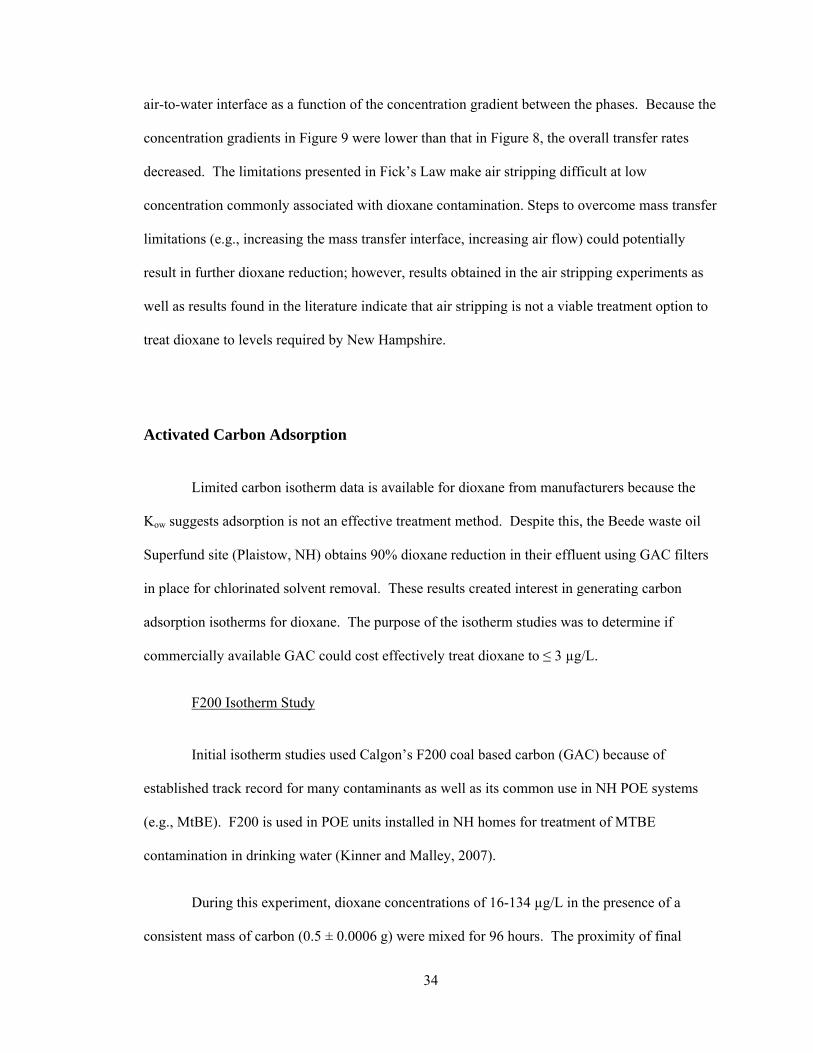
During this experiment, dioxane concentrations of 16-134 µg/L in the presence of a

consistent mass of carbon (0.5 ± 0.0006 g) were mixed for 96 hours. The proximity of final

35

concentrations in the results (despite differences in initial concentrations) indicated equilibrium

between the GAC and aqueous phase dioxane was reached within the 96 hour mixing period

(Figure 10). All subsequent isotherm experiments would use 96 hours as a mixing time to ensure

equilibrium was reached. Controls which lacked GAC were monitored to determine whether

dioxane was lost from solution by means other than carbon adsorption (e.g., improper seals,

sorption to glass). The control samples contained an average of 2.29 ± 2.00% more dioxane at

the end of 96 hours, most likely due to issues with analytical precision.

Results of this experiment (Appendix D) indicated dioxane reductions of 72%, 94%, and

96% in the low, medium, and high standards, respectively (Figure 10). Successful sorption

results in this study encouraged further research on the capacities of dioxane sorption by GAC.

The similarity of final dioxane concentrations (Ce = 4.5, 3.9 and 4.9 µg/L) regardless of

varying initial dioxane concentrations (C0 = 16, 64, and 134 µg/L, respectively) suggested a final

dioxane concentration of ~4-5 µg/L in the aqueous phase. This limit could be due to a limit in

dioxane transport kinetics (e.g., bulk solution transport, film transport, intraparticle transport),

dioxane adsorption limitations (e..g, adsorption mechanism, available sorption sites, GAC

particles size), or competitive adsorption from other solutes found in the groundwater (e.g., iron,

NOM). This limit may possibly be overcome by increasing the contact time, mixing energy, or

changing the adsorbent type, size, or dose. Subsequent GAC experiments further evaluated the

concentration limits of dioxane sorption.

36

Figure 10: F200 Isotherm Study: Final Sorption Evaluation

Sample Type

Low Medium High

1,4-

diox

ane

Con

cent

ratio

n (

g/L)

0

20

40

60

80

100

120

140

160

t = 0 t = 96 hours with F200

134

4.9 3.9

64

4.5

16

37

GAC Comparison Isotherm Study

The purpose of this experiment was to determine the three most effective commercially

available carbons for dioxane sorption for use in further isotherm studies. Seven different types

of GAC were tested representing different manufacturers (Calgon Carbon Corp., Norit Activated

Carbon, TIGG Corp.) and raw base materials (coal, coconut, wood)(Table 12).

Table 12: GAC Type for Comparison Study

Carbon Manufacturer Base Material

Apparent Density (g/cc)

GAC 830 Norit Activated Carbon

Coal 0.50

GCA 830 Norit Activated Carbon

Coconut 0.47

F200 Calgon Carbon Corp.

Coal 0.59

OLC Calgon Carbon Corp.

Coconut 0.48

5DC 830 TIGG Corp. Coconut -

5D 1240 TIGG Corp. Coal 0.43-0.48

5DW 0830 TIGG Corp. Wood 0.24-0.30

Low (13 µg/L) and high (112 µg/L) dioxane concentrations were placed in VOA bottles

with a consistent mass of carbon (0.5 ± 0.0010 g) and mixed for 96 hours. Controls, which

lacked GAC, were monitored to determine whether dioxane was lost from solution due to other

means. The high dioxane control samples attained a 16% reduction in dioxane over the course of

96 hours (Table 13). The likely cause of a significant reduction in the control sample may be

volatilization that occurred during the the post-experiment filtration of the samples to remove

residual GAC. Due to this loss, the initial concentration of the high sample was assumed to be

an average (112 µg/L) of t = 0 and t = 96 hours rather than 102 µg/L or 122 µg/L. The lack of

change seen in the low control sample supports the hypothesis that losses could be attributed to

volatilization, and was seen more dramatically at high concentrations as expected by Fick’s Law.

38

Table 13: Dioxane Concentrations in Controls Lacking GAC

Sample 1,4 dioxane (µg/L) t = 0

1,4 dioxane (µg/L) t = 96 hours

Low 13 13

High 122 102

At the low concentration (13 µg/L), all GAC types, except the wood based carbon (5DW

0830), reduced dioxane concentrations to below the RDL (2.0 µg/L). The wood based carbon

had a low apparent density compared to other GAC types which may have affected the sorption

efficiency. At the high concentration (112 µg/L), dioxane samples showed reductions ranging

from 75-97% (Table 14). GCA 830, F200, and OLC were chosen for continued isotherm testing.

F200 was chosen over the GAC 830 and 5D 1240 (all coal based carbons) because it is

commonly used in NH POE applications for a range of groundwater contaminants.

Table 14: Low and High Concentration for 1,4 Dioxane Removal Results

Activated Carbon Type

1,4 dioxane (µg/L) t = 0

1,4 dioxane (µg/L) t = 96 hours

Percent Reduction

Norit GAC 830 (Coal)

13 < 2 >85% 112 3.6 96.8%

Norit GCA 830 (Coconut)

13 < 2 >85 112 3.8 96.6%

Calgon F200 (Coal)

13 < 2 >85% 112 6.0 94.6%

Calgon OLC (Coconut)

13 < 2 >85% 112 2.8 97.5%

TIGG 5DC 830 (Coconut)

13 < 2 >85% 112 9.5 91.5%

TIGG 5D 1240 (Coal)

13 < 2 >85% 112 8.7 92.2%

TIGG 5DW 0830 (Wood)

13 3.5 >85% 112 27 75.9%

*Graphical representation in Appendix G, percent recovery for each sample in Appendix E

39

GAC Isotherm Experiments

GAC isotherms were created across the range of dioxane concentrations (0-100 µg/L)

typically experienced by POE systems in NH. Preliminary capacities (qe) were calculated (Table

15) for the three types of GAC using Eq. 1. Based on a sample vial size of 67 mL and a carbon

dosage of 0.5 g,

q0.067L 112

μgdioxaneL 6.0

μgL

0.5 F200

= 14.2 μgofdioxane gofF200carbon⁄

Table 15: Initial GAC Capacities for Dioxane

GAC Type Capacity

qe (µg of dioxane/g of carbon) Norit GCA 830

(Coconut) 14.5

Calgon F200 (Coal)

14.2


14.6

Capacities calculated were lower than values found in the literature. Johns et al. (2007) reported

capacities for Filtrasorb 200 (Calgon F200) of ~3,500 µg dioxane/g of activated carbon. The

higher capacity could be due to higher initial dioxane concentration used in their experiment

(800 µg/L vs. 112 µg/L). Differences in experimental design including equalization times,

solution characteristics (e.g., additional contaminants, pH, temperature), and GAC characteristics

(e.g., activation procedure, surface area, density) could also account for dissimilar GAC

capacities. It is important to note that in following the isotherm procedure used by Kinner and

Malley (2007), the calculated capacity of the carbon was not corrected for the use of crushed

carbon, also known as powdered activated carbon (PAC).

40

Using the estimated capacities (Table 15) and rearranging Eq. 1, values were chosen for

initial concentrations (C0) and carbon dosages (M) to provide estimated effluent concentrations

(Ce ) ≈15 µg/L (RDL = 2.0 µg/L), so dioxane could be detected at the end of each isotherm

(Appendix H).

For F200, using Eq. 2, C0 of 100 µg/L will yield a Ce ≈15 µg/L.

C 100µg/L0.4g 14.20

μgL

0.067

15.2 μg/L

Samples for the three select carbon types were filled with calculated initial concentrations

and carbon dosages (Appendix H). These vials were mixed for 96 hours and sampled. Controls

which lacked GAC were monitored to determine whether dioxane was lost from solution due to

other means. Isotherm results (Appendix I) from the 96 hour mixing study were then applied to

the logarithmic Freundlich equation, plotted (Figures 11-13) with a linear regression, and

Freundlich constants calculated (Table 16).

LogarithmicFreundlichEquation:logq1log log

Table 16: Freundlich Isotherm Constants for Three GAC Types

GAC Type KF (95% Confidence Interval)

(80% Confidence Interval)

Norit GCA 830 (Coconut)

9.0 ± 3.2

0.30 ± 0.17

Calgon F200 (Coal)

10.1± 3.3 0.22 ± 0.19


7.8 ± 2.9 0.53 ± 0.10

Because GAC adsorption is not the treatment method of choice for dioxane, published Freundlich

constants are not available for comparison. The coefficient of determination, also known as the

41

R2 value, for Figures 11-13 indicate that the linear regressions do not have a strong fit to the data

for two out of three isotherms. However, due to limited number samples (7) for each isotherm it

was decided that all data points should be included in the regression to avoid altering the

conclusions of the study. To account for the error involved in linear regression, confidence

intervals provide ranges for data associated with the regression analysis.

log Effluent Dioxane Concentration (g/L)

0.0 0.2 0.4 0.6 0.8 1.0

log

Cap

acity

qe

( g/

g)

1.10

1.15

1.20

1.25

1.30

1.35

1.40

y = 0.53x + 0.89

R2 = 0.92

Figure 11: Freundlich Isotherm for OLC

42


0.0 0.2 0.4 0.6 0.8 1.0

log

Cap

acity

qe

( g/

g)

1.10

1.15

1.20

1.25

1.30

1.35

1.40

y = 0.30x + 0.95

R2 = 0.57

Figure 12: Freundlich Isotherm GCA 830

43


0.0 0.2 0.4 0.6 0.8 1.0

log C

apaci

ty q

e (

g/g)

1.10

1.15

1.20

1.25

1.30

1.35

1.40

y = 0.22x + 1.00

R2 = 0.37

Figure 13: Freundlich Isotherm for F200

44

Using the linear regression analysis from each of the isotherm plots, carbon capacities were

calculated using an initial concentration of 20 µg/L. With each new carbon capacity, a 95%

prediction interval was found to determine the range of predicted values at the specific initial

dioxane concentration of 20 µg/L. Applying Freundlich capacities to POE design assumptions

provides projected values for daily carbon usage, exhaustion time, and annual carbon cost for a

single POE unit (Table 17).

Table 17: GAC Comparison for POE Unit

Carbon Capacity at CF = 20

(µg/g)

Carbon Use per day (g)

Exhaustion Time for a 2ft³ POE Reactor (days)

Cost per lb. (2010 quotes)

Annual Carbon Cost

GCA 830 23 ± 9 500-1092 26-57 $1.64 $650-1,400 F200 21 ± 9 537-1263 26-62 $2.12 $900-2,150 OLC 40 ± 12 309-579 47-88 $1.63 $400-750

* For GAC comparison, point-of-entry design assumptions included: C0 = 20 µg/L,CF = 3 µg/L, Q = 250 gpd, POE Reactor volume = 2 ft3, 95% Prediction intervals.

Carbon cost per pound does not include shipping charges which would vary depending on

quantity purchased. It is important to note that this annual cost does not include the capital or

installation cost of the GAC units. Service, GAC re-bedding, and spent GAC disposal for carbon

used for MtBE removal currently costs approximately $275 per unit service visit (McGarry,

2011). For cost estimation purposes, this service value was assumed to be comparable to that of

what dioxane would be. Table 18 outlines estimated drinking water costs including POE unit

service, re-bedding, and GAC disposal based on contracts provided by the NHDES. As expected

for POE systems, the average cost per 1000 gallons treated is significantly higher than the

national average due to the labor costs associated with re-bedding and the large amount of carbon

required for adequate dioxane removal. From the three GAC types compared, OLC (coconut

base, Calgon Carbon Corp.) had the best projected capacity, exhaustion time, and annual cost of

$1,800-3,000 or $20-32 per 1,000 gal treated (Table 18). Drinking water costs were estimated

45

using preliminary GAC isotherm research. For more reliable cost estimation and kinetics

purposes, laboratory column tests (e.g., rapid small-scale column tests (RSSCT)) are considered

more accurate for estimating system performance.

Table 18: Drinking Water Cost

GAC Type Number of Service Re-beds per Year

Annual Estimated Cost per unit

Cost per 1,000 gal. treated

Norit GCA 830 (Coconut) 7-15 $2,500-5,500 $28-61 Calgon F200 (Coal) 6-14 $2,500-6,000 $28-66

Calgon OLC (Coconut) 5-8 $1,800-3,000 $20-32 *National drinking water average = $2 per 1,000 gal. treated

(USEPA, Water On Tap: what you need to know, 2009)

UV Direct Photolysis

The purpose of the UV studies was to determine if direct photolysis could efficiently

degrade dioxane in groundwater to acceptable guidelines of <3 µg/L. Stefan & Bolton (1998)

reported dioxane as a weak absorber of UV light which indicates direct photolysis would not be

successful. Corresponding results were observed by Martijn et al. (2010) finding no significant

degradation of dioxane (C0=200 µg/L) at a UV dosage of 1200 mJ/cm2. However, studies have

shown in natural water systems that UV irradiation can form small amounts of hydrogen

peroxide, a precursor to the hydroxyl radical which has the ability to degrade dioxane (Scully at

al., 1996). For all of the experiments the background UV absorbance of the groundwater

samples was between 0.01-0.03 cm-1.

Initial UV Bench Scale Experiment

The initial UV bench scale study compared two groundwater samples spiked with ~130

µg/L of dioxane over a 25 hour period. One sample was irradiated with a high dosage of UV

46

light (10,000 mJ/cm2), while a control sample was in an environment receiving minimal UV light.

Both samples were stirred during the experiment.

65% and 43% dioxane removals were attained in the irradiated and control samples

respectively (Figure 14). The irradiated sample final concentration was 44 µg/L compared to 75

µg/L in the control sample. The difference between sample removal rates (+22% for the

irradiated sample) was attributed to direct photolysis. Successful direct photolysis contradicts

Stefan & Bolton (1998) and Martijn et al. (2010), however, those experiments did not irradiate

samples at such a high UV dose (1,000 mJ/cm2 vs. 10,000 mJ/cm2). High removal rates in the

control sample indicated dioxane losses through volatilization as observed in the air stripping

study to greater degree (43% vs. 22%). The difference in control sample losses between the

studies may be caused by the difference in mixing mechanisms used in the two experiments:

bubble aeration vs. magnetic stir bar. Control sample results due to volatilization compare

similarly to the ~30% volatilization results found by Bowman et al. (2001) and are logical given

that the sample had to be stirred for 25 hours.

47

Sample Type

1,4-

diox

ane

Con

cent

ratio

n (

g/L)

0

20

40

60

80

100

120

140

UV Dose = 0

UV Dose = 10,000 mJ/cm2

With UV Irradiation Without UV Irradition

Figure 14: Initial UV Bench Scale Experiment

UV Bench Scale Study with Additional Monitoring

A high removal rate in the control sample from the initial experiment indicated some

additional removal mechanism, most likely volatilization from sample agitation. To further

understand removal mechanisms, the experiment was repeated with the addition of a sample

which was neither stirred nor irradiated. Temperature and pH were also measured before and

after the study to ensure that the water chemistry was stable and no other reactions were

occurring. Groundwater samples spiked with ~120 µg/L dioxane were tested over a 25 hour

period. The difference between control samples helped determine if dioxane was volatilizing

without agitation from stirring.

47% dioxane removals were attained in the irradiated and stirred control samples (Figure

15). The similarity of the removal rates of the irradiated and controlled stirred samples indicated

48

little to no effect from direct photolysis as found by Martijn et al. (2010). The sample that was

not stirred or irradiated showed minimal removal (9%) compared to the control sample which was

stirred (47 %). The losses in the control sample compare favorably to those obtained in the initial

UV experiment (43% vs. 47%). These losses indicated that a majority of the dioxane removal

could be attributed to volatilization from the samples being continuously stirred over the course

of the study. Temperature and pH remained relatively consistent between the beginning and the

end of the study (Appendix N).

Sample Type

1,4-

diox

ane

Con

cent

ratio

n (

g/L)

0

20

40

60

80

100

120

140

UV Dose = 0

UV Dose = 10,000 mJ/cm2

UV IrraditionNot stirred

No UV IrraditionNot stirred

UV IrraditionStirred

Figure 15: UV Bench Scale with Additional Monitoring

49

UV Batch Reactor Study

A 5 gallon batch reactor study was used for final consideration of photolysis. A POE-

sized UV reactor (SPV-8 Unit, Trojan Technologies; London, ON) supplied a high UV dose of

19,200 mJ/cm2 over the course of 5 hours at a water flow of 3.78 lpm (1 gpm). A control study

was completed without the UV source on to help determine dioxane losses not attributed to

irradiation.

Without irradiation there was little removed of the 134 µg/L dioxane present with only a

slight variability (5%) over 5 hours (Figure 16). This indicated that there was little to no dioxane

loss from aeration, agitation, or sorption from the closed loop batch reactor. The small variations

in concentration observed may have resulted from incomplete mixing of the dioxane spike or

precision of the analytical method. UV irradiation showed high removal rates at high UV

dosages. A clear dioxane reduction (30%) from an initial averaged concentration of 127.5 µg/L

to a final concentration of 88 µg/L (Figure 16) was observed. However, with high initial dioxane

concentrations and UV dose, the 30% reduction in dioxane from direct photolysis was not

considered viable as a POE technology because of the lack of efficiency. The dioxane reduction

attributed to photolysis at low UV dosages (1,200 mJ/cm2 ) is similar to results reported by

Martijn et al. (2010).

50

UV Dose (mJ/cm2)

0 5000 10000 15000 20000

1,4-

diox

ane

Con

cent

ratio

n (

g/L)

0

20

40

60

80

100

120

140

UVControl

Figure 16: UV Batch Reactor Study with SPV-8 UV Unit

At high UV doses, the possibility of forming of hydroxyl radicals in natural waters

increases due to an increase in the sample’s UV exposure. The generation of hydroxyl radicals in

natural waters can be attributed to several different mechanisms including the photolysis of

hydrogen peroxide, ozone, nitrate, nitrite, dissolved organic matter (DOM), and metal ions

(Brezonik & Fulkerson-Brekken, 1998). Vione et al. (2006) found that DOM was the main

source (and sink) for hydroxyl radicals in a surface water sample while nitrate was the main

source in a groundwater sample. Evaluation of these naturally occuring parameters in NH

groundwater as well a their effects on hydroxyl radical production would be required for further

consideration of direct photolysis.

51


After minimal success with dioxane destruction through direct UV photolysis, hydrogen

peroxide (H2O2) was included in the bench scale studies in an effort to improve removal. Known

for removal of difficult to treat contaminants, UV-peroxide oxidation is an effective AOP able to

treat dioxane levels to < 5 µg/L from an initial dioxane concentration of 367 µg/L (Wojcicka &

Cavalcante, 2004). Dioxane has a favorable second order rate constant for destruction with

hydroxyl radicals at 2.8 × 109 liters/mole•sec (MWH, 2005). However, chemical use (hydrogen

peroxide) and treatment complexities present significant obstacles for application in a POE

system.

Initial UV-Peroxide Experiment

Preliminary testing compared three different groundwater samples spiked with dioxane to

a concentration of 18 µg/L. Samples were spiked with 0, 3, and 6 mg/L H202. The pH and

alkalinity of each sample were monitored before and after the experiment to provide an

estimation of the groundwater hydroxyl scavenging ability. Initial groundwater alkalinity was

measured at 112 ± 2 mg/L as CaCO3. All samples were stirred and irradiated at a UV dose of 600

mJ/cm2, a median dosage applied at existing water treatment facilities (Martijn et al., 2010).

Although the UV dose administered in a POE system has the possiblity to be higher than that

applied at existing water treatment facilities, this initial experiment was conducted to determine

the effectiveness of UV-peroxide using groundwater vs. to pre-treated surface water.

11%, 28%, and 51% reductions in dioxane concentration were observed for the

groundwater samples spiked with 0, 3, and 6 mg/L of hydrogen peroxide, respectively (Figure

17). Dioxane reduction did not meet expectations based on the low initial concentration and high

52

UV-peroxide dosages. Martijn et al. (2010) reported 55% and 57% reduction rates at higher

initial dioxane concentrations (200 µg/L) using similar UV and hydrogen peroxide dosages. The

lack of dioxane destruction was attributed to interferences in the groundwater, specifically

alkalinity (112 ± 2 mg/L as CaCO3) which can act as a scavenger for hydroxyl radicals. Final

dioxane concentrations did not approach the treatment goal of ≤ 3 µg/L in either sample spiked

with hydrogen peroxide.

Sample Type

No H202 With 3 mg/L H202 With 6 mg/L H202

1,4-

diox

ane

Con

cent

ratio

n (

g/L)

0

5

10

15

20

25

UV Dose = 0

UV Dose = 600 mJ/cm2

18 18 18

16

13

8.9

NHDES Guideline

Figure 17: Initial UV-Peroxide Experiment

# above bar = 1,4-dioxane concentration in µg/L

53

UV-Peroxide Experiment for Scavenging Effects

The second UV-peroxide study was designed to determine: a) if the groundwater was

causing hydroxyl interference, and b) if an increased UV and hydrogen peroxide dosage would

result in greater dioxane removal. A reverse osmosis (R.O.) water sample (minimal interferences,

alkalinity < 10 mg/L as CaCO3) spiked to a final dioxane concentration of 13 µg/L was dosed to 3

mg/L hydrogen peroxide and irradiated with a UV dose of 600 mJ/cm2. Groundwater with 13

µg/L of dioxane was spiked with 10 mg/L hydrogen peroxide and irradiated with a UV dose of

1200 mJ/cm2. This treatment represented the high range of dosing for UV-peroxide treatment.

The R.O. water showed > 92% reduction in dioxane concentrations to below an analytical

RDL of 1 µg/L (Figure 18). Martijn et al. (2010) reported similar results (98% removal) when

using Milli-Q water for the sample. These results confirmed that interferences in the

groundwater were inhibiting dioxane degradation. Interferences in dioxane degradation can be

caused by the presence of UV-absorbing compounds or by hydroxyl radical scavengers.

Compounds that absorb UV-light and prevent the formation of hydroxyl radicals include nitrate,

organic matter, and suspended material. Compounds that scavenge hydroxyl radicals and thereby

inhibiting target degradation include carbonate, bicarbonate, reduced metal ions, DOM, and

nitrite. The natural buffering capacity of water (alkalinity) in the form of carbonate (CO32-) and

bicarbonate (HCO3-) species is of particular concern in natural waters because their

concentrations are often three orders of magnitude higher than the target contaminant. Crittenden

et al. reported that even low alkalinities of 50 mg/L (compared to ~112 mg/L CaCO3) reduced the

rate of TCE destruction by a factor of 10 at a pH of 7 (MWH, 2005).

An 82% reduction in dioxane to a final concentration of 2.3 µg/L (Figure 18) was

observed when UV and hydrogen peroxide dosages were increased to 1200 mJ/cm2 and 10 mg/L,

respectively. It is important to note the low initial dioxane concentration (13 µg/L) of dioxane in

54

the samples. Martijn et al. (2010) reported corresponding results (82% removal) at similar UV

and hydrogen peroxide dosages and an initial dioxane concentration of 200 µg/L.

Although UV-Peroxide was able to degrade dioxane to below the NH MCL, there are concerns

regarding its chemical hazard, chemical supply, and lack of record in POE systems. Hydrogen

peroxide at high concentrations used for water treatment (30% w/w) is known to be corrosive as

well as an irritant when in contact with the skin. It also bears an explosion hazard when in the

presence of sparks, heat, acids, metals, or organic materials. At lower concentrations, the

hydrogen peroxide volume required for projected treatment of 250 gpd of water to the NH MCL

exceeds 100 liters annually (Table 19). In addition to concerns of chemical use, hydrogen

peroxide for drinking water treatment requires a post quenching step (e.g. GAC adsorption) for

peroxide removal. Hydrogen peroxide is a strong oxidant and irritant making residual removal a

Figure 18: UV-Peroxide Experiment for Scavenging Effects

Sample Type

1,4-

diox

ane

Con

cent

ratio

n (

g/L)

0

5

10

15

20

25

UV Dose = 0

UV Dose = 600-1200 mJ/cm2

13 13

<12.3

R.O. Water Groundwater

55

mandatory step for drinking water. This ancillary treatment step would add to an already

complex POE UV-peroxide treatment system.

Table 19: Annual Hydrogen Peroxide Use in Liters

Hydrogen Peroxide Strength (w/w)

Q = 946 lpd (250 gpd)

3.3% 10% 30%

Hydrogen Peroxide Dose 3 mg/L 31 10 3 6 mg/L 63 21 7

12 mg/L 105 35 12 *See Appendix R for calculations

The most significant concern with applying UV-Peroxide treatment to a POE unit is that the

process is entirely unproven. The design process would require significant bench, pilot, and full

scale studies before reaching an acceptable safety levels for the public. Although not

recommended for POE use, continued research on UV-peroxide treatment should involve

quantification of hydrogen peroxide doses required for acceptable dioxane concentrations in

groundwater. Variables that could affect hydrogen peroxide dosage include alkalinity, pH,

hydrogen sulfide, metal ions, nitrite, and nitrate.

The use of vacuum UV (VUV) technology has been shown to create hydroxyl radicals

directly from the photolysis of water. Xenon lamps with an emission wavelength of 172 nm have

been shown to enable the oxidation and mineralization of dissolved organic substrates in water

without the addition of chemicals (Oppenlander et al., 2005). More recent studies have indicated

that VUV may be more efficient at generating hydroxyl radicals than other AOPs (Wanget al.,

2010). Although research by Oppenlander & Gliese (2000) has shown that VUV can successfully

mineralize organic micropollutants (e.g., alcohols and phenols), there has been little to no work

done with respect to dioxane. Concerns with VUV include capital cost of the UV source, UV

interferences at low wavelengths (~172 nm), oxidation intermediates, as well as byproduct

formation. Further investigation into VUV would be required before its consideration as a

possible dioxane treatment technology.

56

Chapter 5 – APPLICATIONS FOR RESIDENTIAL TREATMENT

Reductions of dioxane concentrations in groundwater occurred in three out of the four

treatment techniques examined (air stripping, GAC adsorption, UV-peroxide). However,

treatment capabilities and process efficiency limit which techniques may be applied in residential

settings. This section is intended as a guide to choosing the appropriate POE technology based on

water characteristics (e.g., dioxane concentration, alkalinity). Research completed on these

techniques was preliminary, focusing on the feasibility of each process instead of optimization.

As a result, pilot-scale testing is recommended for all technologies before residential application.

Air Stripping

Air stripping through diffused bubble aeration was not effective at removing dioxane (≤ 3

µg/L) from groundwater at low initial concentrations (20-30 µg/L), indicating that this

technology should not be used exclusively for POE treatment. However, preliminary stripping

experiments with high dioxane concentrations (> 100 µg/L) and high A:W ratios (5000:1)

reduced dioxane concentrations by as much as 39%. Further research into the overall feasibility

and economics of air stripping is necessary to validate and reinforce these findings. In addition,

other types of aeration not tested (e.g., fine bubble, pressurized in-line aeration, spray aeration)

may prove to be more effective at removing dioxane than the methods applied in this research.

If stripping is applied in a POE unit, strict emissions control is necessary. Care must be

taken to ensure that dioxane emissions do not accumulate where the unit is installed (e.g., cellar)

or where the off-gas pipe is located (e.g., roof), as dioxane vapors can be harmful to the user. In

addition to emissions control, clogging and fouling issues should be investigated before

installation. Groundwater characteristics such as iron (Fe+2, Fe+3), manganese (Mn+2), nutrients,

57

and hardness should be measured. Groundwater concentrations of ferrous iron are particularly of

concern in NH groundwater, as this compound can precipitate when oxidized (Sutherland &

Adams, 2004). Clogging of groundwater aeration units (diffused bubble) has been observed with

the likely culprit being iron precipitates (Kinner, Malley Jr., & Clement, 1990). Increased levels

of nutrients (e.g., nitrate) can cause biofouling problems in the stripping system.

Many of the clogging and fouling issues associated with air stripping can be minimized

with proper maintenance and monitoring practices. Pretreatment practices (e.g., ion exchange,

GAC) may be applied to reduce the effects of iron, manganese, and hardness. However, the

investigation of radionuclides must be completed for GAC adsorption pretreatment processes to

ensure there is no danger of long term accumulation (gamma emissions) (Kinner, Malley Jr., &

Clement, 1990).

GAC Adsorption

Adsorption using GAC was effective at removing dioxane from groundwater below the

NH MCLG of 3µg/L. All GACs, which were of a coal or coconut base, were able to treat

dioxane to <3 µg/L. From the carbons tested (Table 12), OLC (coconut base, Calgon Carbon

Corp.) provided the highest capacity at 38 µg of dioxane/g of OLC carbon. Filtrasorb 200 (coal,

Calgon Carbon Corp.), commonly used in NH POE applications, provided a capacity of 20 µg of

dioxane/g of F200 carbon. GAC capacities were based on an influent concentration of 20 µg/L.

This research indicated that a coconut based carbon may yield better dioxane sorption results in

GAC units than coal based carbons, although costly ($20-32 per 1,000 gal. treated, Table 18).

Assuming a common GAC POE reactor volume of 2ft3, dioxane breakthrough would occur in as

short of a time as 1.5 months, requiring re-bedding. The safe practice would be to install a

second POE unit in series with the first to guard against drinking water contamination from any

58

unit failure. Breakthrough times could also be increased through the expansion of the typical

GAC POE reactor volume which is commonly 2ft3,

Because GAC indiscriminately adsorbs many solutes, design must take into account other

species present in the groundwater (e.g., natural organic matter (NOM), hydrogen sulfide, and

other radionuclides). These compounds, along with other organic and inorganic pollutants, may

compete for adsorption sites on the GAC or clog the bed. If present, further investigation of

radon and radionuclides must be completed in to ensure there is no danger of long term

accumulation (gamma emissions) on the GAC (Kinner, Malley Jr., & Clement, 1990).

Similar to air stripping, GAC performance may be hindered by iron hydroxide and

manganese oxide precipitation, calcium carbonate scaling (CaCO3), and biofouling. Evaluation

of iron (Fe+2, Fe+3), manganese (Mg+2), hardness (Ca+2, Mg+2), and pH would be required for

pretreatment considerations. Ion exchange pretreatment may help alleviate issues associated with

manganese, iron, and calcium carbonate. However, the investigation of radionuclides must be

completed in ion exchange pretreatment processes to ensure there is no danger of long term

accumulation (gamma emissions). Past studies on MtBE removal using POE GAC systems in

New Hampshire indicate that these issues are not likely sources of serious concern for 1,4

dioxane treatment because the shorter exhaustion rate (< 6 months vs. 1 year). However, these

parameters still need to be addressed before a POE system is implemented.


Direct photolysis was not proven to reduce dioxane concentrations in groundwater and

therefore should not be considered as a treatment option.

59

UV-Peroxide

UV-peroxide advanced oxidation was not found to be efficient at reducing dioxane

concentrations in groundwater. The NH MCLG (3 µg/L) was only accomplished with low (13

µg/L) initial dioxane concentrations and a high dose of UV (1200 mJ/cm2) and hydrogen

peroxide (10 mg/L). Efficient dioxane destruction was not observed likely due to interferences in

the groundwater (e.g., hydroxyl radical scavenging, UV absorbance). Groundwater

characteristics such as alkalinity, NOM, metal ions (Fe+2, Mg+2), and hydrogen sulfide (H2S)

determine if hydroxyl radicals produced will likely be scavenged (MWH, 2005). Of these

characteristics, alkalinity is likely to be one of the most common obstacles for UV-peroxide

treatment. The natural buffering capacity of water (alkalinity) in the form of carbonate (CO32-)

and bicarbonate (HCO3-) species is of particular concern in natural waters because their

concentrations are often three orders of magnitude higher than the target contaminant. Crittenden

et al. reported that even low alkalinities of 50 mg/L (compared to ~112 mg/L) reduced the rate of

TCE destruction by a factor of 10 at a pH of 7 (MWH, 2005).

Chemical doses coupled with a required hydrogen peroxide post-quenching step make

UV-peroxide a complicated application in a POE residential treatment system. However, the

most significant concern with applying UV-Peroxide treatment to a POE unit is that the process is

entirely unproven. The design process would require significant bench, pilot, and full scale

studies before being accepted for use in a residential POE system.

.

60

Chapter 6 – CONCLUSIONS

Air Stripping

Contrary to what the dimensionless Henry’s Law Constant of 1.96 × 10-6 (Howard, 1990)

indicates, dioxane exhibits some degree of volatilization from water. Air stripping was

proven to significantly reduce dioxane concentrations in groundwater (39%) when initial

concentrations were high (> 100 µg/L). However, high reduction rates required high

A:W ratios (5000:1) and were not proven to reach levels below 26 µg/L.

Air stripping was not found to be effective at removing dioxane from groundwater when

1) initial dioxane concentrations were closer to values which POE systems would

experience (20-30 µg/L), 2) the required final concentrations were low (≤ 3 µg/L), and 3)

when A:W ratios were realistic (240:1).

GAC Adsorption

GAC adsorption studies indicate that 6 out of the 7 carbons tested were able to treat

dioxane to < 2.0 µg/L in groundwater. Dioxane adsorption was most successful in

coconut and coal based carbons. Only the wood based carbon (5DW 0830) was not able

to treat to this level.

Isotherm studies for OLC, F200, and GCA carbons indicated short exhaustion times

between 26 and 88 days for a 2 ft3 POE unit with 250 gpd flow and an influent dioxane

concentration of 20 µg/L.

OLC was the most efficient carbon tested, resulting in a single POE unit exhaustion time

of between 47-88 days at an annual carbon cost of $550.

Further evaluation (pilot scale) of coconut based carbon (e.g., OLC) is recommended

based on the isotherm results which compare coal and coconut capacities.

61


UV direct photolysis was found to be ineffective at degrading dioxane in groundwater at

high doses of UV light (10,000 mJ/cm2). In both Bench Scale Study A and Study B, a

majority (42.7- 46.8%) of the total dioxane reduction (47.3-65.1%) could be attributed to

volatilization from the samples being stirred. This conclusion compares favorably with

the air stripping results.

The UV Batch Reactor Study confirmed the ineffectiveness of direct photolysis showing

only 31.0% dioxane reduction using a UV dose (19,200 mJ/cm2) at a high initial dioxane

concentration (127.5 µg/L). Assuming this removal rate, the influent dioxane

concentration to a POE unit would need to be ≤ 9.7 µg/L to reach the NH MCLG of 3

µg/L.


UV-Peroxide was not found to effectively degrade low concentrations (< 20 µg/L) of

dioxane in groundwater at typical and high dosages of hydrogen peroxide (3-10 mg/L)

and UV irradiation (600-1200 mJ/cm2). Control samples in the UV-Peroxide studies

indicate that groundwater interferences such as alkalinity (117 mg/L as CaCO3) greatly

inhibit dioxane degradation by scavenging hydroxyl radicals.

Compounds that scavenge hydroxyl radicals and thereby inhibiting target degradation

include carbonate, bicarbonate, reduced metal ions, DOM, and nitrite.

62

Chapter 7 –Recommendations

Air Stripping

Further research on air stripping is not recommended when initial dioxane concentrations

are low (20-30µg/L), as seen in many New Hampshire aquifers.

Air stripping may be a viable pre-treatment option in cases where the initial dioxane

concentration is high (> 100 µg/L). In these cases, air stripping could be a cost effective

pre-treatment option to decrease the operating costs of the primary treatment technology

(e.g., carbon adsorption).

GAC Adsorption

Further evaluation of coconut based carbon is recommended based on the isotherm

results. Laboratory column tests (e.g., rapid small-scale column tests (RSSCT)) could

provide a more accurate prediction of GAC performance in a POE system.


UV direct photolysis is ineffective at degrading dioxane in groundwater. Further

research is not recommended.


UV-Peroxide is not a viable POE option for the treatment of dioxane in groundwater

because the technology is unproven in this application. Significant testing would need to

be completed to validate UV-Peroxide as an acceptable POE treatment system for

dioxane.

63

REFERENCES Abe, A. (1998). Distribution of 1,4-dioxane in Relation to Possible Sources in the Water Environment. The Science of the Total Environment , 41-47.

Adams, C. D. (1994). Oxidation and Biodegradability Enhancement of 1,4-Dioxane Using Hydrogen Peroxide and Ozone. Environmental Science and Technology , 1812-1818.

Aitchison, E. W., Kelley, S. L., J, A. J., & Schnoor, J. L. (2000). Phytoremediation of 1,4-Dioxane by Hybrid Poplar Trees. Water Environmental Research , 313-321.

ATSDR. (2007, September). Public Health Statement for 1,4 Dioxane. Retrieved January 12, 2010, from Agency for Toxic Substances and Disease Registry: http://www.atsdr.cdc.gov/PHS/PHS.asp?id=953&tid=199

ATSDR. (2007, September). Toxicological Profile for 1,4 Dioxane. Retrieved January 12, 2011, from Agency for Toxic Substances and Disease Registry: http://www.atsdr.cdc.gov/toxprofiles/tp.asp?id=955&tid=199

Black, R. E., Hurley, F. J., & Havery, D. C. (2001). Occurence of 1,4-Dioxane in Cosmetic Raw Materials and Finished Cosmetic Products. Journal of the AOAC , 666-670.

Bolton, J. (2004, May 6). Germicidal Fluence (UV Dose) Calculations for Low Pressure UV Lamp (Excel Spreadsheet). Edmonton, Alberta, Canada.

Bolton, J. (2005, May 6). Germicidal FLuence (UV Dose) Calculations for Low Pressure UV Lamp (Excel Spreadsheet). Edmonton, Alberta, Canada.

Bolton, J. R., & Linden, K. G. (2003). Standardization of Methods for Fluence (UV Dose) Determination in Bench-Scale UV Experiments. Journal of Environmental Engineering , 209-215.

Boltz, D. F., & Howell, J. A. (1978). Colorimetric Determination of Nonmetals. New York: Wiley-Interscience.

Bowman, R. H. (2001). Ozone-Peroxide Advanced Oxidation Water Treatment System for Treatment of Chlorinated Solvents and 1,4-Dioxane. Applied Process Technology, Inc.

Brezonik, P. L., & Fulkerson-Brekken, J. (1998). Nitrate-Induced Photolysis in Natural Waters: Controls on Concentrations of Hydroxyl Radical Photo-Intermediates by Natural Scavenging Agnets. Environmental Science and Technology , 3004-3010.

CHEMFATE. (2003). Syracuse Research Corporation.

Doherty, R. E. (2000). A History of the Production and Use of Tetrachloride, Tetrachloroethylene, Trichloroethylene, and 1,1,1-Trichloroethane in the United States: Part 2-Trichloroethylene and 1,1,1-Triochloroethane. Journal of Environmental Forensics , 83-93.

Dow, C. C. (1954). Patent No. 2,811,252. The United States.

64

Earth Tech, Inc. (2004). Technology evaluation for treatment of 1,4-dioxane in groundwater. Tuscno, AZ: Air Force Center for Environmental Excellence.

Eddy; Metcalf; AECOM. (2007). Water Reuse. New York, NY: McGraw-Hill Companies.

Esso Research and Engineering, C. (1967). Patent No. 3359331. The United States.

Howard, P. H. (1990). Handbook of Environmental Fate and Exposure Data for Organic Chemicals. Chelsea, MI: Lewis Publishers, Inc.

Johns, M., Wayne, M. E., & Toles, C. A. (1997). Agricultural By-products as Granular Activated Carbons for Adsorbing Dissolved Metals and Organics. The Journal of Chemical Technology and Biotechnology , 131-140.

Kano, H., Ulmeda, Y., Tatsuya, K., & Toshiaki, S. (2009). Carcinogenecity studies of 1,4-dioxane administered in drinking-water to rats and mice for 2 years. Food and Chemical Toxicology , 2776-2784.

Kim, Y. H., & Engesser, K. H. (1994). Degradation of Alkyl Ethers, Aralkyl Ethers, and Dibenzyl Ether by Rhodococcus sp. Strain DEE5151, Isolated from Diethyl Ether-Containing Enrichment Culture. Applied and Environmental Microbiology , 4527-4530.

Kinner, N. E., Malley Jr., J. P., & Clement, J. A. (1990). Radon Removal Using Point-of-Entry Water Treatment Techniques. Cincinnati, OH: U.S. EPA.

Kinner, N., & Malley, J. P. (2007). GAC Point-of-Entry Treatment System Generation of Tertiary Butyl Acohol (TBA) During Methyl tert-Butyl Ether (MtBE) Treatment of Groundwater. Durham, NH: Environmental Research Group.

Lagrega, M. D., Buckingham, P. L., & Evans, J. C. (2001). Hazardous Waste Management. New York, NY: McGraw-Hill.

Linden, K., & Rosenfeldt, E. (2010). Water Quality & Treatment, 6th Ed. Chapter 18. McGraw-Hill.

Lyman, W. J., & Rosenblatt, D. H. (1982). Handbook of Chemical Property Estimation Methods. New York, NY: McGraw-Hill Book Co.

Mahendra, S., & Alvarez-Cohen, L. (2005). Pseudonocardia dioxanivorans sp. nov., a novel actinomycete that grows on 1,4 dioxane. International Journal of Evolutionary Microbiology , 593-598.

Malley, J. P. (2011, June 23). Radiometer Calibration. (M. Curry, Interviewer)

Martijn, B. J., Fuller, A. L., Malley, J. P., & Kruithof, J. (2010). Impact of IX-UF Pretreatment on the Feasiblity of UV/H202 Treatment for Degradation of NDMA and 1,4-Dioxane. Ozone: Science and Engineering , 32: 6, 383-390.

65

McGarry, F. (2009, September). 1,4-dioxane POE Design Specifications. (N. Kinner, & M. Curry, Interviewers)

Mohr, T. K. (2001). 1,4-Dioxane and other Solvent Stabilizers White Paper. Santa Clara Valley Water District.

Mohr, T. K. (2010). Environmental Investigation and Remediation: 1,4-Dioxane and Other Solvent Stabilizers. CRC Press.

Montgomery Watson Harza. (2005). Water Treatment: Principles and Design. Hoboken, NJ: John Wiley & Sons, Inc.

Mzurkiewicz, J., & Tomasik, P. (2005). Why 1,4-dioxane is a water-structure breaker. Journal of Molecular Liquids , 111-116.

National Cancer Institute. (1978). Bioassay of 1,4-Dioxane for Possible Carcinogenecity. Bethesda, MD: The U.S. Department of Health, Education, and Welfare.

NHDES. (2008, October). Innovative Land Use and Planning Techniques: A Handbook For Sustainable Development. Retrieved January 10, 2011, from New Hampshire Department of Environmental Services: http://des.nh.gov/organization/divisions/water/wmb/repp/innovative_land_use.htm

Oppenlander, T., Gliese, & S. (2000). Mineralization of organic micropollutants in water by vacuum-UV-oxidation with an incoherent xenon-excimer lamp at 172 nm. Chemosphere , 15-21.

Oppenlander, T., Walddorfer, C., Burgbacher, J., Kiermeier, M., & Weinschrott, H. (2005). Improved vacuum-UV (VUV)-initiated photomineralization of organic compounds in water with a xenon excimer flow-through photoreactor containing an axially centered ceramic oxygenator. Chemosphere , 302-309.

Parales, R. E., Adamus, J. E., White, N., & May, H. D. (1994). Degradation of 1,4-Dioxane by an Actinomycete in Pure Culture. Applied and Environmental Microbiology , 4527-4530.

Powell, T. (2010, January 8). Photo-cat quote. (M. Curry, Interviewer)

Riddick, J. A., Bunger, W. B., & Sakano, T. K. (1986). Organic Solvents: Physical Properties and Methods of Purification. New York, NY: Wiley-Interscience.

Scully, N., McQueen, D. R., & Cooper, W. J. (May 1996). Hydrogen Peroxide Formation: The Interaction in Ultraviolet Radiation of Dissolved Organic Carbon in Lake Waters. Limnology and Oceanography , 540-548.

Shangraw, T., & Plaehn, W. (2006). Full-Scale Treatment of 1,4-Dioxane USing a Bioreactor. Federal Remediation Technologies Roundtable Meeting (pp. 11-12). Arlington: Engineering Management Support, Inc. and Parsons Corporation.

66

Stefan, M. I., & Bolton, J. R. (1998). Mechanism of the Degradation of 1,4-Dioxane in Dilute Aqueous Solution Using the UV/Hydrogen Peroxide Process. Environmental Science and Technology , 1588-1595.

Steffan, R. J. (August 2007). ER-1422: Biodegradation of 1,4-Dioxane. Tuscon, AZ: SHaw Environmental, Inc.

Sutherland, J., & Adams, C. (2004). Treatment of MTBE by air stripping, carbon adsorption, and advanced oxidation; technical and economic comparison for five groundwaters. Water Research , 38: 193-205.

USEPA. (2009, October). 2009 Edition of Drinking Water Standards and Health Advisories. Retrieved November 12, 2010, from www.epa.gov: http://water.epa.gov/action/advisories/drinking/upload/dwstandards2009.pdf

USEPA. (2010, August 19). Ozone Layer Protection. Retrieved December 13, 2010, from www.epa.gov: http://www.epa.gov/ozone/intpol/

USEPA. (2009, December). Water On Tap: what you need to know. Retrieved from http://www.epa.gov/ogwdw000/wot/pdfs/book_waterontap_full.pdf

Vione, D., Falleti, G., & Maurino, V. (2006). Sources and Sinks of Hydroxyl Radicals upon Irradiation of Natural Water Samples. Environmental Science and Technology , 3775-3781.

Wang, D., Oppenlander, T., Gamel El-Din, M., & Bolton, J. R. (2010). Comparison of the Disinfection Effects of Vacuum-UV and UV Light on Bacillus subtilis Spores in Aqueous Suspensions at 172, 222, and 254 nm. Photochemistry and Photobiology , 176-181.

Weber, W. J. (1972). Physicochemical Processes For Water Quality Control. New York, NY: Wiley-Interscience.

Wojcicka, L., & Cavalcante, N. (2004). Treatment of 1,4-Dioxane in Groundwater using Advanced Oxidation Processes: UV/Peroxide, Ozone/Peroxide, and UV/Titanium Dioxide.

Zenker, M. J. (2004). Biodegradation of 1,4-Dioxane Using a Trickling Filter. Journal of Environmental Engineering , 926-931.

Zenker, M. J., Borden, R. C., & Baralz. (2003). Occurence and Treatment of 1,4-Dioxane in Aqueous Environments. Environmental Engineering Science , 423-432.

Zenker, M. J., Borden, R. C., & Barlaz, M. A. (2000). Mineralization of 1,4-dioxane in the presence of a structural analog. Biodegradation , 239-246.

67

Appendix A: Literature Review

The objective of this research, set by the NHDES, was to evaluate possible POE

treatment technologies for the reduction of dioxane in private groundwater systems. This

appendix reviews the literature available on different processes used to remove dioxane (dioxane)

from water along with their potential applicability to POE systems. The review covers the public

health and regulatory aspects of dioxane, as well as specific treatment processes including air

stripping, activated carbon adsorption, bioremediation, and oxidation. It should be noted that

much of literature involves large scale processes (>1,000 gpd) which may not be applicable for a

POE (<250 gpd) system (McGarry, 2009). The applicability of a process to POE treatment will

be discussed along with its dioxane removal efficiency and the test conditions under which they

were achieved. Many of the publications evaluated several processes. Therefore, the same

reference will be listed in several sections.

Public Health Effects

In 2007, the Agency for Toxic Substances and Disease Registry (ATSDR) completed a

toxicological profile of dioxane noting exposure can occur from inhalation of contaminated air,

ingestion of contaminated drinking water or food, and dermal contact (ATSDR, 2007). Limited

information is available on dioxane’s direct health effects on humans. However, extensive

research on animals (e.g., rats, mice, guinea pigs) provides sufficient evidence that the liver and

kidneys are the target organs for toxicity (Kano et al., 2009).

68

Existing Studies

Figure 19: Available1,4 Dioxane Health Effect Studies (ATSDR, 2007)

69

A Minimum Risk Level (MRL) is defined as an estimate of daily human exposure to a substance

that is likely to be without an appreciable risk of adverse non-carcinogenic effects over a

specified duration of time (Table 20).

Table 20: Minimum Risk Levels for Humans as a Result of Exposure to 1,4 Dioxane (Adapted from ATSDR)

Exposure Type Duration Minimum Risk Level (MRL)

MRL in Drinking Water*

Inhalation Acute 2 ppm - Chronic 1 ppm -

Oral

Acute 4 mg/kg/day 140,000 µg/L Intermediate 0.6 mg/kg/day 21,000 µg/L

Chronic 0.1 mg/kg/day 3,500 µg/L Acute: <14 days Intermediate: 14-365 days Chronic: >365 days

*Assuming 2L of water per day and an average body weight of 70 kg (Appendix S)

Most groundwater sites are contaminated at relatively low concentrations (µg/L) compared to

concentrations used in toxicity studies (mg/L). Chronic (low concentration, long duration)

exposure risk may be more appropriate than acute (high concentration, short duration), especially

with respect to drinking water. Chronic two year exposure to dioxane in drinking water was

linked to liver cancer in rats and mice (Kano et al, 2009).

Air Stripping

Preliminary research on dioxane’s properties reveals a low Henry’s Law constant (KH) of

4.88 × 10-6 atm m3/mole coupled with high solubility. The key property controlling the transport

of dioxane is its solubility. The high solubility of dioxane (Figure 20) can be attributed to the two

oxygen atoms (in red) which are available for interaction with water molecules (Mzurkiewicz &

Tomasik, 2005).

70

The combination of a high solubility with a low Henry’s law constant makes air stripping

ineffective at removing dioxane from water (Mohr, 2001). However, some case studies have

shown limited success in dioxane stripping from water. Air stripping may not be viable to use as a

sole method to reduce dioxane to regulatory limits, but it could be effective in combination with

other processes.

Bowman et al. (2001) investigated the effectiveness of an air stripper as pre-treatment for

an AOP to remove chlorinated solvents in Industry, CA. The air stripper was run at 10 gpm, pH

range of 7.2-8.6. The average removal efficiency for dioxane was 29.5% with influent and

effluent concentrations of 610 and 430 µg/L, respectively.

A case study at U.S. Air Force Plant 44 (Tucson, AZ) to determine if existing large-scale

air strippers, designed to remove chlorinated solvents, could be adjusted to remove dioxane.

Influent dioxane concentrations were 10-15 µg/L with a target effluent concentration of 6 µg/L.

The treatment system consisted of three parallel trains of two stage air stripping towers (primary

and secondary) with a design flow of 5,000 gpm. When the primary and secondary towers were

operated at air to water ratios of 7:1 and 25:1, respectively, no dioxane was removed. When air

Figure 20: 1,4-Dioxane Model

(Oxygen = Red Carbon = Black Hydrogen = White)

71

to water ratio were increased to 69-291:1 a maximum dioxane removal rate of ~10% was

achieved. (Earth Tech, Inc., 2004)

The limited studies done on dioxane removal as well as the variable results for air

stripping indicate that while this technology may be applied to POE units, attaining low effluent

concentrations (≤ 3 µg/L) may be difficult.


The octanol-water partition coefficient (Kow) for dioxane suggests that carbon adsorption

techniques will not be effective. However, granular activated carbon (GAC) systems designed to

remove volatile organic compounds (VOCs) at the Beede waste oil site (Plaistow, NH) have

shown as recently as August 2009, a 90% reduction in dioxane concentrations (35 µg/L to 3.4

µg/L) (Pea09). GAC manufacturers do not have isotherm data for dioxane, making it difficult to

predict the characteristics of a POE activated carbon system.

The dioxane removal efficiencies of GAC produced from agricultural by-products (e.g.,

rice straw, soybean hull, peanut, pecan, walnut shells) were compared to that of commercial

carbon (e.g., Filtrasorb 200 and Centaur 20 × 50; Calgon Carbon Corporation; Pittsburgh, PA)

(Johns et al., 1997). A mixed suite of six organic compounds was employed testing (benzene,

toluene, dioxane, acetonitrile, acetone, methanol). In the study, 0.1 g of carbon are added to a 10

mL organic solution containing 800 µg/L of each compound. Carbon adsorption was the lowest

for dioxane. It also had the greatest variability in removal rates. Estimations made from the

organics adsorption graph (Figure 1 in the paper) showed carbon capacities for Filtrasorb 200

(F200) and Filtrasorb 400 (F400) of ~3,500 µg dioxane/g carbon. However, only the GAC

produced from walnut and pecan shells exceeded 50% dioxane removal. Commercial grade GAC

72

showed removal rates in the 40% range. The reduced affinity for dioxane compared to the other

compounds was attributed to competition with the other adsorbates (e.g., benzene, toluene,

acetonitrile, acetone, methanol. Fortunately, at residential sites where dioxane is a concern, it is

the sole organic contaminant present.

At a groundwater contamination site in South El Monte, CA, the local water authority

conducted monitoring on a GAC system which consisted of two 20,000 lb carbon reactors. The

groundwater was contaminated with a variety of chlorinated solvents as well as dioxane. The

system was run at 9.7 gpm to help reduce 1,1-DCA contamination (Bowman, 2001). It failed to

significantly reduce the dioxane concentrations which averaged 20 µg/L.

Local success at the Beede Waste Oil site (Plaistow, NH) shows GAC is capable of

treating dioxane to below regulatory limits (≤ 3 µg/L). The low water demand of a household

POE system (≤ 250 gpd) meant a multi-pass low flow GAC system could treat dioxane to

required regulatory levels. Such POE adsorption units are common in the home water treatment

industry. A GAC system could also be used in series with another process technology (e.g., air

stripping) to attain better dioxane removal. Future application of GAC for dioxane removal from

groundwater depends on carbon exhaustion rates. Research needed includes the development of

isotherms in order to determine GAC POE re-bedding frequency and cost.

Bioremediation

Dioxane is widely thought to be recalcitrant to microbial activity under normal

environmental conditions, but some studies have found success. Bioremediation studies

involving dioxane as the sole substrate as well as by co-metabolism (i.e., primary substrate =

tetrahydrofuran (THF), propane) have been reported (Shangraw & Plaehn, 2006). Co-metabolic

studies have shown greater success than when dioxane was the sole substrate.

73

THF (Figure 21), an industrial solvent, is the most common primary substrate used with

dioxane due to similarity in structure. However, THF is not usually a co-contaminant with

dioxane in residential situations, so it would need to be added to stimulate biodegradation.

However, THF addition for co-metabolism is not practical in POE applications.

Figure 21: Tetrahydrofuran

1,4 Dioxane as Sole Substrate

In 1993, Parales et al. reported a bacterium (Actinomycete CB1190) capable of

aerobically growing on dioxane as its sole carbon and energy source after being gradually weaned

from a THF enrichment. Direct enrichments on dioxane were unsuccessful; CB1190

preferentially degraded THF in a pure culture. The bacteria were initially isolated from an

industrial waste sludge produced at a dioxane-contaminated site in Darlington, SC. At 30°C, the

pure culture had a specific activity of 0.33 mg of dioxane per min per mg of microbial protein

and mineralized ~50% of the dioxane to CO2. No other organic intermediates were found in the

samples after dioxane degradation. Successful biodegradation of dioxane in this study was only

found with gradual, long term enrichments. THF still was definitely the preferred substrate of the

isolated CB1190 culture.

74

Confirmation of Parales’ results on the CB1190 strain came in 2005 (Mahendra &

Alvarez-Cohen). Using the same pure culture that was isolated from the dioxane-contaminated

industrial sludge and supplied by Parales, growth was achieved using dioxane as the sole

substrate in aerobic conditions. Growth continued for up to 28 days at an optimal temperature of

30°C.

In 2004, Kim and Engesser isolated 20 strains from sewage sludge (Stuttgart, Germany)

which were known to degrade ethers as a sole carbon and energy source, including 18

Rhodococcus strains and two Sphingomonas strains. Strains were aerobically incubated at 30°C.

None of the 20 isolates were able to grow on dioxane or THF.

These studies indicate that bioremediation using dioxane as a sole carbon source is a

difficult process to maintain making it unlikely to be applied successfully to a POE unit.

1,4 Dioxane as a Co-Metabolite

A complete, fullscale study of dioxane and THF biodegradation in groundwater was

performed at the Lowry Landfill Superfund site (Denver, CO). THF is an obligate co-metabolite

in dioxane biodegradation. Promising bench-scale reductions in dioxane (73%) and THF (88%)

concentrations led to a pilot study with parallel 300 gal., fixed film, moving bed bio-reactors to

study the effects of temperature (25° and 15°C). The full scale system was designed with three

aerobic, fixed film, moving bed bio-reactors able to reduce dioxane concentrations (C0=25,000

µg/L) to ≤ 1 µg/L using indigenous bacteria (Flow rate = 6 gpm, Temperature = 23°C) (Shangraw

& Plaehn, 2006). In this study, oxygen was the electron acceptor and dioxane (or THF) the

electron donor.

75

Zenker et al. (2004) designed a laboratory scale trickling filter to biodegrade cyclic ethers

including dioxane and THF at concentrations encountered in contaminated groundwater. Using

oxygen as the electron acceptor and dioxane (or THF) as the electron donor, the filter was

operated for 1 year at low (200 µg/L) and medium (1,000 µg/L) influent dioxane loading. The

average air flow rate through the filter was 0.17 L/min with a hydraulic residence time of 14.4

minutes. At low loading levels with THF present, the filter was capable of consistent dioxane

biodegradation to ~2-10 µg/L. However, the system was more effective at removing THF due the

bacteria’s greater affinity for it as compared to dioxane. The biodegradation of dioxane was

inhibited with the presence of THF in the system until the primary substrate (THF) reached

relatively low levels. This competitive inhibition is commonly observed in co-metabolic

processes where two substrates (dioxane and THF) are competing for the same enzyme.

In a study funded by the U.S. Department of Defense, Steffan (2007) used two aquifers to

show that dioxane was recalcitrant when a primary substrate (propane or THF) was not present.

It did not matter whether aerobic, nitrate, iron, or sulfate reducing or methanogenic conditions

existed. dioxane was not degraded in any of the anaerobic microcosms over >400 days.

Biodegradation of dioxane was observed after >100 days in microcosms of strain ENV478 which

had been stimulated with propane and THF. This and previous studies demonstrate that

biological treatment and natural attenuation are unlikely to be successful remedial choices for

sites contaminated with dioxane, unless a suitable primary substrate is present.

Phytoremediation

In 2000, Aitchison et al. successfully showed that hybrid poplar trees (Populus deltoids,

DN34-Imperial California) effectively removed dioxane from soil and water. The poplar trees

76

were able to remove 54.0 ± 19.0% of a 23,000 µg/L solution of dioxane after 9 days of exposure

through uptake and translocation. The hybrid cuttings also remediated contaminated soil (10

mg/kg) leaving only 18.8 ± 7.9% of the original dioxane in the soil after a 15 day exposure. In

both experiments, a majority of the dioxane assimilated by the poplars was transpired through the

leaves into the air where it was photo degraded. It is important to note that this experiment only

involved short-term results on relatively young poplar plants (8-12 weeks). Although a promising

soil remediation solution, phytoremediation would be difficult to apply to a drinking water

application.

Advanced Oxidation Processes

Advanced oxidation of dioxane is the most common process employed in industrial waste

situations, however, the use of hazardous chemicals make it difficult to apply to a POE system

Common AOPs for dioxane make use of ultraviolet irradiation (UV), hydrogen peroxide (H2O2),

ozone (O3), titanium dioxide (TiO2) in different combinations to mineralize dioxane. Listed

below in Table 19 in are common AOPs used for dioxane:

Table 21: Advanced Oxidation Processes for 1,4 Dioxane Removal In Water

Advance Oxidation Process Acronym Pilot Study Manufacturer Hydrogen Peroxide with Ultraviolet Irradiation

H2O2 + UV Trojan Technologies, Inc (London, Ontario, Canada)

Ozone with Hydrogen Peroxide

O3+ H2O2 HiPOx®, Applied Process Tech. (Long Beach, CA)

Titanium Dioxide with Ultra-Violet Irradiation

TiO2 + UV Purifics ES Inc. (London, Ontario, Canada)

Advanced Oxidation Processes (AOPs) work by creating hydroxyl radicals, highly

reactive species, through the combination of different chemicals and catalysts. These processes

require careful monitoring, expensive equipment, and the use of costly chemicals which make

77

them undesirable for use in a POE system. Developed AOP technologies can treat dioxane

concentrations to drinking water standards (< 3µg/L) at sites where there is a need for a large

scale treatment system (Table 20).

Table 22: Advanced Oxidation Processes for 1,4 Dioxane Treatment

Advanced Oxidation Process

Untreated conc. (µg/L)

Treated conc.(µg/L)

Source

O3 + H2O2 470 <2 (Bowman, 2001)

UV + H2O2 >70 7 (Stefan & Bolton, 1998)

UV + TiO2 3,000 8 (Wojcicka & Cavalcante, 2004)

In 2004, Wojcicka & Cavalante completed a comprehensive study comparing the ability

of these three AOPs (O3 + H2O2, UV + H2O2, UV + TiO2) to be added to a groundwater treatment

plant and treat dioxane in groundwater. The parameters monitored during the study included

hydroxyl radical scavenging potential, general water characteristics, and by-product formation

(i.e., bromate from bromide in ozone treatment). The results from the initial bench-scale study

concluded that the scavenging potential was the most important water characteristic to evaluate

due to its effect on AOP efficiency. The pilot-scale study used systems supplied and optimized

by manufacturers in the water treatment industry. All three AOP systems were evaluated in

parallel after the water was pre-chlorinated (to oxidize metals and rejuvenate filter media) and

filtered just as at the water treatment plant. dioxane was reduced in all three systems from 47-151

µg/L to a targeted concentration of < 10 µg/L when the systems were optimized (number of UV

lamps on, flow rates, chemical dosing).

78

Stefan and Bolton (1998) conducted experiments which were able to define the

degradation routes for dioxane when treated with a dilute aqueous H202 solution (30%) and

ultraviolet (UV) light as the catalyst for hydroxyl radical generation (UV + H2O2). After 5 min.

irradiation with UV light, 90% removal was achieved. They noted pH adjustments may be

required because the pH was 4.2 after treatment. The reactor volume used was 28 L recirculated

at 110 L/min.. Difficulties with applying this process to a POE system lie in the chemical

requirements of hydrogen peroxide, a strong oxidant which must be handled with care. However,

if only low dosages of H2O2 are required, this may be feasible and effective. Further bench scale

research regarding source water characteristics (dioxane concentration, scavenging abilities) are

needed to determine UV + H2O2 viability in a POE unit.

In 2001, Bowman completed an O3 + H2O2 pilot study with support from the San Gabriel

Basin Water Quality Authority using a HiPOx® system from Applied Process Technology, Inc.

(Long Beach, CA). The pilot test was performed in South El Monte, CA at a site contaminated

with chlorinated solvents and dioxane (20.2 µg/L). The pilot unit was run at 10 gpm with H2O2

and O3 influent concentrations of 6.90 mg/L and 3.12 mg/L, respectively. The optimized H2O2

and O3 dosages resulted in an effluent dioxane concentration of < 2 µg/L. This case study also

cited two other groundwater contamination sites where the implementation of an ozone and

hydrogen peroxide system were able to reduce the dioxane concentration to < 3 µg/L. The on-site

generation of O3 in this pilot study means it cannot be applied to a POE system for cost and safety

concerns.

A photocatalytic oxidation evaluation was completed in 2005 using a Photo-Cat®

treatment system supplied by Purifics ES, Inc. (London, Ontario, Canada). This new system uses

UV light to activate titanium dioxide (TiO2 ) beads which act as a catalyst to produce hydroxyl

radicals. The Photo-Cat® was capable of treating dioxane concentrations of ~150 µg/L to below

detection limit of 1.9 µg/L , a near 99% reduction. The results also showed that by-product

79

production (i.e., bromate) is not of concern when using this treatment technology. High costs

make photocatalytic presently undesirable for POE treatment. Laboratory systems capable of

treating 250 gpd were quoted at $70,000, with an operation cost of ~$1.00 per day (Powell,

2010).

80

Appendix B: F200 Isotherm Studies-Initial Sorption Evaluation Data

Table 23: F200 Initial Sorption Concentration Results

Sample 1,4 Dioxane Concentration (µg/L)

t = 0 hrs, No GAC t = 96 hrs, No GAC t = 96 hrs, With GAC % Removal Groundwater Blank 6.3 (110%) 5.8 (113%) < 2.0 (115%) - Low Conc. - 15 µg/L 20¹ (113%) 18 (111%) 2.1 (111%) 90 Med. Conc. - 60 µg/L 21 (119%) 20 (118%) < 2.0 (108%) > 90 High Conc. - 120 µg/L 29 (114%) 27 (112%) 2.7 (107%) 91

¹Sample spike = 54 µg/L (112%)

Table 24: Mass of F200 for Initial Sorption

F200 Carbon Measured (g)

0.5000

0.5000

0.5006

0.5002

0.4999

0.5002

0.5002

0.5004

0.4999

0.5002

0.4999

0.5000

0.4998

0.5004

0.5005

0.5005

0.5000

Average (g) 0.5002

Std. Dev. (g) 0.00025

81

Appendix C: F200 Isotherm Studies-Revised Sorption Evaluation Data

Table 25: F200 Revised Sorption Concentration Results


t = 0 hrs, No GAC t = 96 hrs, No GAC t = 96 hrs, With GAC % Removal Groundwater Blank

3.8 (108%) 4.7 (106%) < 2.0 (102%) -

Low Conc. 15 µg/L

12¹ (95%) 11 (109%) 2.3 (108%) 81

Med. Conc. 60 µg/L

44 (103%) 42 (108%) 2.3 (103%) 95

High Conc. 120 µg/L

84 (107% 83 (106%) 5.2 (105%) 94

¹Sample spike = 37 µg/L (102%)

Table 26: Mass of F200 for Revised Sorption


0.4990

0.5000

0.4990

0.5000

0.5000

0.5002

0.5004

0.5000

0.5000

0.5003

0.5000

0.5002

0.5002

0.5005

0.5000

0.5002

0.5000

Average (g) 0.5000

Std. Dev. (g) 0.00041

82

Appendix D: F200 Isotherm Studies: Final Sorption Evaluation Data

Table 27: F200 Final Sorption Concentration Results


t = 0 hrs, No GAC t = 96 hrs, No GAC t = 96 hrs, With GAC % Removal Groundwater Blank <2.0 (112%) <2.0 (112%) <2.0 (108%) - Low Conc. - 15 µg/L 16 (110%) 16 (109%) 4.5 (111%) 72 Med. Conc. - 60 µg/L 64 (119%) 66 (118%) 3.9 (112%) 94 High Conc. - 120 µg/L 134 (121%) 139 (113%) 4.9 (118%) 96

Table 28: Mass of F200 for Final Sorption


0.5020

0.5000

0.5010

0.5000

0.5000

0.5000

0.5010

0.5000

0.5010

0.5000

0.5010

0.5000

0.5010

0.5010

0.5000

0.5001

0.5000

Average (g) 0.5005

Std. Dev. (g) 0.0006

83

Appendix E: GAC Comparison Isotherm Study Data

Table 29: Standard Concentrations for GAC Isotherm Study

t = 0 hrs t = 96 hours Average

High Conc. Standard-µg/L 122 (131%) 102 (112%) 112

Low Conc. Standard-µg/L 13 (117%) 13 (117%) 13

Table 30: GAC Comparison Results After 96 Hour Mixing

Types of Activated Carbon

1,4 Dioxane Concentration

Groundwater Blank with GAC

Low Conc.-µg/L (13 µg/L at t = 0)

High Conc. -µg/L (122 µg/L at t = 0)

GAC 830 <2.0 (125%) <2.0 (128%) 3.6 (109%)

GCA 830 <2.0 (116%) <2.0 (127%) 3.8 (124%)

F200 <2.0 (105%) <2.0 (128%) 6.0 (107%)

OLC <2.0 (122%) <2.0 (136%) 2.8 (148%)

5DC 830 <2.0 (135%) <2.0 (124%) 9.5 (112%)

5D 1240 <2.0 (124%) <2.0 (119%) 8.7 (121%)

5DW 0830 <2.0 (113%) 3.5 (116%) 27 (117%)

84

Appendix F: Initial Carbon Capacity Estimations

Using the High 96 hour concentration data from the initial GAC comparison isotherm study,

estimated capacities (qe) were calculated using Equation 1 for the three most promising carbon

types:

Table 31: Dioxane Concentrations for Initial GAC Comparison Study

96 Hour Mixing Test: Carbon Types

Concentration F200 5D 1240 GAC 830 5DC OLC GCA 830 5DW

Blank - - - - - - -

Low <2 <2 <2 <2 <2 <2 3.5

High 6.0 8.7 3.6 9.5 2.8 3.8 27

Carbon Base Coal Coconut Wood

*Yellow indicates that the GAC was chosen for further testing, GCA 803 (coconut base) was

chosen over GAC 830 (coal base) for continued testing because F200 showed comparable results

and was considered the industrial standard for coal based carbon in water treatment.

Example for F200:

Equation1:C C

0.067 112 6.0μgL

0.5 200

14.20

200

85

Appendix G: GAC Comparison for Dioxane Sorption

Figure 22: High Initial Concentration GAC Comparison Graph

Figure 23: Low Initial Concentration GAC Comparison Graph

0

20

40

60

80

100

120

F200 5D 1240 GAC 830 5DC OLC GCA 830 5DW

1,4

Dio

xan

e C

onc.

(p

pb

)

Carbon Types

High Conc. 96 Hour Mixing ResultsInitial High Conc. (102 ppb) Conc. After Mixing

0

2

4

6

8

10

12

14

F200 5D 1240 GAC 830 5DC OLC GCA 830 5DW

1,4

Dio

xan

e C

onc.

(p

pb

)

Carbon Types

Low Conc. 96 Hour Mixing ResultsInitial Low Conc. (13 ppb) Conc. After Mixing

86

Appendix H: Carbon Dosage Requirements Calculations

Table 32: F200 Carbon Dose Requirements

For F200 where

qe(µg/g)= 14.20 C0 (µg/L) M (g) Volume (L) Ce (µg/L)

100 0.4 0.067 15.2 80 0.3 0.067 16.4 60 0.2 0.067 17.6 40 0.1 0.067 18.8 20 0.025 0.067 14.7

Table 33: OLC Carbon Dose Requirements

For OLC where

qe(µg/g)= 14.63 C0 (µg/L) M (g) Volume (L) Ce (µg/L)

100 0.4 0.067 12.64 80 0.3 0.067 14.48 60 0.2 0.067 16.32 40 0.1 0.067 18.16 20 0.025 0.067 14.54

Table 34: GCA 830 Carbon Dose Requirements

For GCA 830 where qe(µg/g)= 14.50

C0 (µg/L) M (g) Volume (L) Ce (µg/L) 100 0.4 0.067 13.44 80 0.3 0.067 15.08 60 0.2 0.067 16.72 40 0.1 0.067 18.36 20 0.025 0.067 14.59

87

Appendix I: GAC Isotherm Experimental Data

Table 35: Concentration of Dioxane Standards

Standard (µg/L) Time (hours) Conc. - µg/L

(Percent Recovery) Averaged Conc.

µg/L

100 t = 0 89 (118%)

89.5 t = 96 90 (122%)

80 t = 0 68 (128%)

71.0 t = 96 74 (121%)

60 t = 0 53 (123%)

52.5 t = 96 52 (116%)

40 t = 0 39 (118%)

36.0 t = 96 33 (110%)

20 t = 0 16 (120%)

16.0 t = 96 16 (119%)

Groundwater Blank t = 96 <1.0 (114%) ‐

Table 36: Dioxane Isotherm Results for OLC

OLC C0 (µg/L) Carbon (g) Ce (µg/L) Capacity

(µg dioxane/g carbon)

OLC Blank - 0.50000 <2.0 (117%) -

OLC 20 16.0 0.02510 7.8 (122%) 21.9

OLC 20 Replicate 16.0 0.02510 7.5 (119%) 22.7

OLC 40 36.0 0.10053 5.0 (121%) 20.7

OLC 60 52.5 0.20030 4.1 (122%) 16.2

OLC 80 71.0 0.30127 3.6 (122%) 15.0

OLC 100 89.5 0.40028 3.4 (121%) 14.4

OLC 100 Replicate 89.5 0.40028 3.2 (115%) 14.5

88

Table 37: Dioxane Isotherm Results for GCA

GCA C0 (µg/L) Carbon (g) Ce (µg/L) Capacity


GCA Blank - 0.50000 <2.0 (119%) -

GCA 20 16.0 0.02502 9.6 (120%) 17.1

GCA 20 Replicate 16.0 0.02502 9.8 (121%) 16.6

GCA 40 36.0 0.10083 7.6 (112%) 18.9

GCA 60 52.5 0.20077 5.8 (117%) 15.6

GCA 80 71.0 0.30033 5.1 (118%) 14.7

GCA 100 89.5 0.40063 5.7 (118%) 14.0

GCA 100 Replicate 89.5 0.40063 5.2 (118%) 14.1

Table 38: Dioxane Isotherm Results for F200

F200 C0 (µg/L) Carbon (g) Ce (µg/L) Capacity


F200 Blank - 0.50000 <2.0 (100%) -

F200 20 16.0 0.02520 10 (116%) 16.0

F200 20 Replicate 16.0 0.02520 10 (115%) 16.0

F200 40 36.0 0.10013 8.0 (119%) 18.7

F200 60 52.5 0.20077 5.7 (116%) 15.6

F200 80 71.0 0.30050 5.7 (114%) 14.6

F200 100 89.5 0.40075 5.8 (111%) 14.0

F200 100 Replicate 89.5 0.40075 5.4 (120%) 14.0

89

Date of this Version 06-May-04

Germicidal Fluence (UV Dose) Calculations for a Low Pressure UV LampProgrammed by Jim Bolton - Bolton Photosciences Inc., 628 Cheriton Cres., NW, Edmonton, AB, Canada T6R 2M5

Tel: 780-439-4709 (home); 519-741-6283 (cellular); Fax: 780-439-7792; Email: [email protected] and/or questions are welcome

Note that this Spreadsheet includes the new "Divergence Factor", which has been found to be necessary due to the fact that the beam "diverges" as it passes through the solution.

Note: This Spreadsheet should only be used if the suspension depth in the "Petri" dish is greater than 2 cm.For suspensions with depths less than 2 cm, use the Spreadsheet "Fluence - LP - shallow.xls"

DO NOT CHANGE ANY CELLS OTHER THAN THE CELLS WITH A YELLOW BACKGROUND

INSTRUCTIONS AND NOTES 1. Set up a "quasi" collimated beam apparatus. If possible, do not use a "collimating tube", but rather use circular "masks" to define the beam. Make sure that safety measures are taken to protect workers from exposure to the UV from the lamp. EYE PROTECTION IS AN ABSOLUTE REQUIREMENT. 2. Place the detector head of the UV radiometer on a horizontal surface, containing a 0.5 cm x 0.5 cm grid, such that the "calibration plane" (see the Calibration Sheet provided by the manufacturer of the Radiometer) is at the level of where the top of the solution will be during exposures to the UV. 3. Determine the "Petri Factor" using the procedure given in the "Petri Factor" Worksheet. 4. Measure the absorption coefficient (1 cm absorbance) at 254 nm for the water to be irradiated and insert into Cell C43. Make sure that the instrument is balanced with distilled water in the same cuvette. 5. Insert the solution volume into Cell F34. 6. Insert the distance from the center of the UV lamp to the surface of the water in the Petri Dish into cell F36. 7. Insert the center meter reading into cell G46. 8. Insert the desired Fluences (UV Doses) into cells E55 to E61. 9. Remove the radiometer detector head and place a Petri Dish (or other container), containing the cell suspension, on a stirring motor placed so that the top of the solution is at the same level as that of the "calibration plane" of the detector head. Add a very small stir bar and make sure that the stirring rate is such that there is no vortex. 10. Expose samples in the UV beam for the times calculated in rows 55 to 61. Do at least three exposures for each time and in random order. 11. The "example" Worksheet shows how to analyze the data and obtain the Fluence (UV Dose) Response Curve.

solution volume = 150 mLwater path length = 3.90 cm

distance from UV lamp to top of water surface = 43.8 cm

absorption totalcoefficient absorbance Water Factor

cm-1 (A) X Divergence Factor

0.0250 0.097 0.824717

Radiometer reading at the center of Petri Dish = 0.140 mW/cm2

Petri factor = 0.968

True irradiance across the Petri dish = 0.136 mW/cm2

Reflection factor = 0.975Water factor *

Divergence factor = 0.825

Average Germicidal Irradiance throughout the water volume = 0.109 mW/cm2

Time for a Fluence (UV Dose) of 1 mJ/cm2 = 9.178 s

Time for a Fluence (UV Dose) of 7,000 mJ/cm2 = 64243.2 s = 1070 min 43 s = 17.83 hours




Time for a Fluence (UV Dose) of 0 mJ/cm2 = 0.0 s = 0 min 0 s = 0 hours



Note: the exposure times should be at least 1 min. If they are calculated to be shorter, arrange the irradiation platform further away from the UV lamp so that the irradiance will be smaller.

Appendix J: IUVA-Bolton Photosciences Spreadsheet (Low Pressure-Deep Sample)

Figure 24: Bolton Photosciences Excel Spreadsheet

90

Appendix K: Preliminary Air Stripping Test Data

Table 39: Preliminary Air Stripping Results

Sample Type 1,4 Dioxane Concentration (µg/L)

Sample Time (hrs)

0 1 4 8 12 25

Non-Aerated (Controls) 104 (104%) - - 80 (105%) - 81 (104%)

Aerated 104 (104%) 105 (106%) 93 (109%) - 65 (111%) 41 (106%) Aerated Groundwater Blank

5.5 (107%) - - - - <2.0

(112%)

Table 40: Air:Water Ratios for 150 mL Sample at 500 sccm

Time (hrs) Time (min.) Total Air Supplied in scc's

(@ Q=500 sccm*) A:W Ratios for a 150 mL Sample

0 0 0 0

1 60 30,000 200

4 240 120,000 800

8 480 240,000 1600

12 720 360,000 2400

25 1500 750,000 5000 *Standard cubic centimeters per minute

91

Appendix L: Primary Air Stripping Test Data Using Typical A:W Ratios

Determination of sampling times at a flowrate within the range (0-500 sccm) of the U201 Matheson flowmeter

Table 41: Primary Air Stripping Results at Typical A:W Ratios

Sample Type 1,4 Dioxane Concentration (µg/L)

Sample Time (hrs)

0 0.5 1 2 4 6 Non-Aerated (Controls)

31 (125%) - - 30 (113%) - 27 (117%)

Aerated

31 (125%) 29 (113%) 28 (124%) 30 (111%) 28 (119%) 26 (114%)

Aerated Groundwater Blank

<2.0 (113%) - - - - <2.0 (117%)

Table 42: Air:Water Ratios for 150 mL Sample at 100 sccm

Time (hrs) Time (min.)

Total Air Supplied in scc's (@ Q=100 sccm*)

A:W Ratios for a 150 mL Sample

0 0 0 0

0.5 30 3,000 20

1 60 6,000 40

2 120 12,000 80

4 240 24,000 160

6 360 36,000 240 *Standard cubic centimeters per minute

92

Appendix M: Initial UV Bench Scale Study Data

Table 43: Initial UV Bench Scale Results (Percent Recovery)

Time (hours) Sample Type 0 25.5 % Removal Irradiated and Stirred-µg/L 126 (102%)* 44 (100%) 65.1 Not Irradiated and Stirred-µg/L 131 (97%) 75 (93%) 42.7 R.O. Blank- µg/L 5.2 (100%) -

*Estimated concentration because the sample exceeded the calibration curve upper limit

93

Appendix N: UV Bench Scale Study with Additional Monitoring Data

Table 44: UV Bench Scale Study Results with Additional Monitoring

Time (hours) Sample Type 0 24 % Removal

Not Irradiated or Stirred - µg/L 105 (140%) 96 (105%) 8.6

Not Irradiated, Stirred- µg/L 126 (122%) 67 (113%) 46.8

Irradiated and Stirred- µg/L 112 (116%) 59 (131%) 47.3

Not Irradiated, Sealed- µg/L 112 (121%) 113 (105%) -0.9

Table 45: pH and Temperature Data for UV Bench Scale Study with Additional Monitoring

Not Irradiated, Not Stirred

Not Irradiated,

Stirred

Irradiated, Stirred

Not Irradiated,

Sealed

Temp. Before Experiment (°C) 18 18 18 18

Temp. After Experiment(°C) 19.5 19.5 20 19.5

pH Before Experiment 7.8 7.9 7.9 7.9

pH After Experiment 8.1 8.3 8.2 7.9

94

Appendix O: UV Batch Reactor Study Data

Table 46: Batch Control Study Results

Time (hrs) Inlet Conc. -µg/L Outlet Conc. -µg/L % Difference Inlet and Outlet Avg.

Conc. -µg/L

0 133 (123%) 135 (119%) 1.5% 134

1 134 (121%) 130 (124%) -3.1% 132

2 133 (135%) 133 (122%) 0.0% 133

3 131 (116%) 128 (121%) -2.3% 128

4 139 (112%) 134 (124%) -3.7% 137

5 138 (121%) 144 (106%) 4.2% 141

*UV Batch Blank < 2.0 µg/L

Table 47: UV Batch Reactor Study Results

Time (hrs)

Inlet Conc. µg/L

Outlet Conc. µg/L

Avg. Conc. µg/L

% Difference UV Dosage¹

(mJ/cm2)

0 133 (131%) 122 (124%) 127.5 -9.0% 0

1 124 (125%) 122 (118%) 123 -1.6% 3,840

2 113 (130%) 111 (127%) 112.25 -2.3% 7,680

3 102 (119%) 102 (116%) 102 0.0% 11,520

4 95 (112%) 97 (116%) 96 2.1% 15,360

5 88 (115%) 88 (113%) 88 0.0% 19,200 *Groundwater Blank < 2.0 µg/L

¹Output from Bolton Spreadsheet (LP-Deep)

95

Appendix P: Initial UV-Peroxide Experiment Data

Table 48: Initial UV-Peroxide Results

UV Dosage (mJ/cm2) 1,4 Dioxane Concentration (µg/L)

No H202 With 3 mg/L H202 With 6 mg/L H202 0 18 (113%) 18 (116%) 18 (113%)

600 16 (123%) 13 (117%) 8.9 (123%)

Table 49: Alkalinity for Initial UV-Peroxide Experiment

UV Dosage (mJ/cm2)

Alkalinity (mg/L as CaCO3)

No H202 With 3 mg/L H202 With 6 mg/L H202 0 110 112 110

600 112 115 110

Table 50: pH for Initial UV-Peroxide Experiment

UV Dosage (mJ/cm2) No H202 With 3 mg/L H202 With 6 mg/L H202 0 8.1 8.2 8.1

600 8.4 8.4 8.4

Table 51: Hydrogen Peroxide Concentration for Initial UV-Peroxide Experiment

UV Dosage (mJ/cm2) Hydrogen Peroxide Conc. (mg/L)

No H202 With 3 mg/L H202 With 6 mg/L H202 0 - 3 6

600 - 3 5.5

96

Appendix Q: UV-Peroxide Experiment Data for Scavenging Effects

Table 52: UV-Peroxide Results for Scavenging Effects (Percent Recovery)

1,4 Dioxane Concentration (µg/L) R.O. Water Groundwater

UV Dosage (mJ/cm2)

No UV or H202

With 3 mg/L H202

No UV or H202

With 10 mg/L H202

0 13 (118%) 13 (118%) 13 (123%) 13 (123%) 600-1200 13 (121%) <1.0 (112%) 14 (111%) 2.3 (119%)

Table 53: Alkalinity Results for UV-Peroxide Experiments for Scavenging Effects

Alkalinity (mg/L as CaCO3) R.O. Water Groundwater

UV Dosage (mJ/cm2)

No UV or H202

With 3 mg/L H202

No UV or H202

With 10 mg/L H202

0 0 - 116 116 600-1200 0 0 112 120

Table 54: pH Results for UV-Peroxide Experiment for Scavenging Effects

R.O. Water Groundwater UV Dosage (mJ/cm2)

No UV or H202

With 3 mg/L H202

No UV or H202

With 10 mg/L H202

0 4.9 - 7.6 - 600-1200 5.3 5.4 8.5 8.6

Table 55: Hydrogen Peroxide Results for UV-Peroxide Experiment for Scavenging Effects

R.O. Water Groundwater UV Dosage (mJ/cm2)

No UV or H202

With 3 mg/L H202

No UV or H202

With 10 mg/L H202

0 - 3 - >10 600-1200 - 3 - >10

97

Appendix R: Hydrogen Peroxide Dosing Calculations

Example:

Using 3.3% hydrogen peroxide for a dose of 3 mg/L:

365 946 3 33,000 31

Hydrogen Peroxide % (w/w) 3.3 10 30

Concentration (mg/L) 33,000 100,000 300,000

Hydrogen Peroxide Dose (mg/L)

3 31 10 3

6 63 21 7

12 126 41 14

98

Appendix S: MRLs for Humans Converted to Drinking Water Levels

Assumptions: 2 L of drinking water/day

Average adult = 70 kg

Oral Exposure (Acute)

MRL = 0.4

0.4 70

28

28 ×

14

99

Appendix S: Laboratory Percent Recovery Correction Calculation

High recovery rates of the surrogate standards triggered the NHDES laboratory to begin reporting 1,4 dioxane concentration as adjusted concentrations. Dioxane concentrations were corrected based on the percent recovery of a surrogate standard, in our case, deuterated-1,4dioxane with the following equations:

%

100%

100%%

Date post:	30-Apr-2018
Category:	Documents
Upload:	vananh
View:	220 times
Download:	3 times

1,4 DIOXANE REMOVAL FROM GROUNDWATER … · Appendix F: Initial Carbon Capacity Estimations ... 1,4...

Documents