1438 IEEE TRANSACTIONS ON COMPUTERS, VOL. 54, NO. 11, NOVEMBER

Causality-Based Predicate Detectionacross Space and Time

Punit Chandra and Ajay D. Kshemkalyani, Senior Member, IEEE

Abstract—This paper presents event stream-based online algorithms that fuse the data reported from processes to detect causality-

based predicates of interest. The proposed algorithms have the following features. 1) The algorithms are based on logical time, which

is useful to detect “cause and effect” relationships in an execution. 2) The algorithms detect properties that can be specified using

predicates under a rich palette of time modalities. Specifically, for a conjunctive predicate �, the algorithms can detect the exact fine-

grained time modalities between each pair of intervals, one interval at each process, with low space, time, and message complexities.

The main idea used to design the algorithms is that any “cause and effect” interaction can be decomposed as a collection of

interactions between pairs of system components. The detection algorithms, which leverage the pairwise interaction among the

processes, incur a low overhead and are, hence, highly scalable. The paper then shows how the algorithms can deal with mobility in

mobile ad hoc networks.

Index Terms—Predicates, event streams, causality, data fusion, time, space-time, mobility, ad hoc network, intervals, monitoring.

�

1 INTRODUCTION

EVENT-BASED data streams represent relevant statechanges that occur at the various processes that are

monitored in a distributed system. The paradigm ofanalyzing event streams using data fusion to detectpredicates of interest to various applications is rapidlygaining importance. This paper proposes online algorithmsfor detecting causality-based predicates and behavioralpatterns using event streams which are generated bypotentially mobile processes across the system.

Stable global predicates (once a stable predicate becomestrue, it remains true) can be detected using techniques suchas snapshot algorithms [9]. However, unstable globalpredicates are difficult to detect. This is because aninstantaneous observation across various locations is notpossible due to the lack of perfectly synchronized clocks.Furthermore, the asynchronous nature of the distributedsystem—caused by unpredictable propagation delays andCPU loads, unknown scheduling policies, and mobility—leads to many interleavings of the events and differentobservations of their order. Hence, it is important to have aframework to specify various temporal modalities on thepredicates on the various distributed variables and tomonitor these predicates.

Two modalities, Possiblyð�Þ and Definitelyð�Þ, for thesatisfaction of a global predicate � in a distributed executionwere defined by Cooper and Marzullo [12] and are widelyaccepted [11]. Informally, Possiblyð�Þ/Definitelyð�Þ is trueif some/every observation of an execution will passthrough a state in which � is true. These two modalitiesare based on the potential causality or the “happens before”

relation in distributed executions, which was defined byLamport [24].

The formalism and axiom system given in [19] identifieda complete, orthogonal set < of 40 fine-grained temporalrelations or interaction types (i.e., modalities) on time intervalpairs, based on the potential causality relation in adistributed execution. Any two intervals at two processesare related by one and only one relation in < and no relationin < can be expressed in terms of others in <. It has beenshown [20] that this formalism provides much moreexpressive power than the Possibly and Definitely modalitiesand a mapping from < to the Possibly and Definitely

modalities has been given.A conjunctive predicate is of the form

Vi �i, where �i is

any predicate defined on variables local to process Pi. (Anexample is: xi ¼ 5

Vyj > 2.) The local durations in which �i

is true naturally identify intervals of interest at process Pi inan execution. We model such intervals as the “meta-events”that give rise to the “event stream” generated by eachprocess. Information about the reported intervals is “fused”or correlated and examined in one of the following ways:

. To detect global states of the execution that satisfy agiven predicate.

. To analyze causal relations between intervals to“data mine” patterns in the behavior.

The earliest global state in which a conjunctive predicateholds is well-defined due to the lattice structure of the set ofglobal states [28]. We show that, for a conjunctive predicate�, Possiblyð�Þ and Definitelyð�Þ can be detected along withthe added information of the exact interaction type from <between each pair of intervals, one interval at each process.This provides flexibility and power to monitor eventstreams generated from different mobile processes. Thetime, space, and message complexities of the proposedonline, detection algorithms (Algorithms Fine Poss andFine Def) to detect Possibly and Definitely in terms of the

1438 IEEE TRANSACTIONS ON COMPUTERS, VOL. 54, NO. 11, NOVEMBER 2005

. The authors are with the Computer Science Department, 851 S. MorganSt., University of Illinois at Chicago, Chicago, IL 60607.E-mail: {pchandra, ajayk}@cs.uic.edu.

Manuscript received 27 May 2004; revised 14 Mar. 2005; accepted 15 July2005; published online 16 Sept. 2005.For information on obtaining reprints of this article, please send e-mail to:[email protected], and reference IEEECS Log Number TC-0222-0705.

0018-9340/05/$20.00 � 2005 IEEE Published by the IEEE Computer Society

fine-grained modalities per pair of processes are the same asthose of the earlier online algorithms [15], [16] that candetect only whether the Possibly and Definitely modalitieshold. In addition, the proposed algorithms work in mobilead hoc networks. Fine Rel, which is an intermediateproblem we need to solve, is addressed first. Fine Rel isimportant in its own right because it determines a globalstate such that a prespecified fine-grained modality for eachpair of processes is satisfied. We also consider the problemAll Pairs Fine Rel to detect the fine-grained relationbetween each pair of intervals from different processes.The output can be useful in analyzing causal relations andmining behavioral patterns in the execution.

We now formally define the problems for which wedesign efficient online algorithms that fuse informationfrom the event streams provided by (potentially) mobileprocesses/nodes.

Problem Fine Rel statement. Given a relation ri;j from <for each pair of processes Pi and Pj, identify the intervals(if they exist), one from each process, such that eachrelation ri;j is satisfied for the ðPi; PjÞ pair.

Problem Fine Poss statement. For a conjunctive predicate�, determine online if Possiblyð�Þ is true. If true, identifythe fine-grained pairwise interaction ri;j from < betweeneach pair of processes ðPi; PjÞ when Possiblyð�Þ firstbecomes true.

Problem Fine Def statement. For a conjunctive predicate �,determine online if Definitelyð�Þ is true. If true, identifythe fine-grained pairwise interaction ri;j from < betweeneach pair of processes ðPi; PjÞ when Definitelyð�Þ firstbecomes true.

Problem All Pairs Fine Rel statement. Devise an onlinealgorithm to determine which relation from < holdsbetween each pair of intervals from different processes.

The proposed algorithms detect “cause-effect” relation-ships from the information in event streams, using pre-dicates under a rich palette of temporal specifications. Theperformance of the algorithms is compared in Table 1. P0 isthe data fusion server that processes the event streams. Themetrics are the average time complexity at P0, the totalspace complexity at P0, the cumulative size of all themessages sent to P0, the network-wide count of the

messages sent by the processes to P0, and the averagespace at each process Pi. The parameters n, M, p, ms, andmr are explained in the legend.

For Fine Rel, Fine Poss, and Fine Def , all the mea-sures at P0 are either linear or quadratic in n, the size of thead hoc network. This indicates high scalability of thealgorithms. More importantly, the size of the spacerequirement at each process Pi (i 2 ½1; n�), which is bothspace and energy constrained in a mobile ad hoc network, islinear in n, the number of mobile processes. This makes thealgorithm easily implementable. The overhead can befurther lowered by using a hierarchical structuring of thead hoc network into clusters, with the data fusion server atits root. Known algorithms for managing various issues dueto migration and mobility [2], [3], [4], [26], [30], [32] can beused in conjunction to maintain the hierarchical clusterorganization.

The paper is organized as follows: Section 2 gives thebackground and objectives. Section 3 gives the frame-work and data structures. Sections 4, 5, and 6 give theonline detection algorithms. Section 7 shows how thealgorithms can run on mobile ad hoc networks. Section 8gives the concluding remarks and discusses furtherresearch challenges.

2 MODEL AND BACKGROUND

2.1 System Model

The system model is broad enough to accommodate not justtraditional distributed computing environments, but alsomobile ad hoc networks. The model assumes a looselycoupled ad hoc asynchronous message-passing system inwhich any two processes belonging to the process set N ¼fP1; P2; . . . ; Png can communicate over logical channels. Fora wireless communication system, a physical channel existsfrom Pi to Pj if and only if Pj is within Pi’s range; a logicalchannel is a sequence of physical channels representing amultihop path. Explicit mobility is permitted in the modeland both processes and nodes can migrate within the adhoc network. The only requirement is that each process beable to send its gathered data eventually and asynchro-nously (via any routes) in a FIFO stream to a system-wideknown data fusion server. Known techniques for managingmobility and clustering can be used within a mobile ad hoc

CHANDRA AND KSHEMKALYANI: CAUSALITY-BASED PREDICATE DETECTION ACROSS SPACE AND TIME 1439

TABLE 1Comparison of Space, Message, and Time Complexities

n = number of processes,M = maximum queue length at P0, p = maximum number of intervals occurring at any process,ms = number of messagessent by all the processes, mr = number of messages received by all the processes. Note: 1) p � M as all the intervals may not be sent to P0.2) ms ¼ mr for unicasts.

network. In the remainder of this paper, the term “process”will be used to denote a mobile process. We assume that a

single process runs at each node; thus, node mobility andprocess mobility also become synonymous.

Ei is the linearly ordered set of events executed byprocess Pi in an execution. An event executed by Pi is

denoted ei. An execution is modeled as ðE;�Þ, where E ¼Si Ei is the set of all the events and � is the potential

causality or the “happens before” relation, defined as thetransitive closure of the local ordering relation on each Ei

and the ordering imposed by message send events andmessage receive events [24]. A cut C is a subset of E suchthat if ei 2 C then ð8e0iÞ e0i � ei¼)e0i 2 C. Thus, the events

of a cut are downward-closed within each Ei. A consistent

cut is a downward-closed subset of E. Only all downward-

closed subsets of E preserve causality and denote correctlyobservable execution prefixes.

A variable x local to process Pi is denoted as xi. Given a

networkwide predicate on the variables, the intervals ofinterest at each process are the durations during which thelocal predicate is true. Such an interval at process Pi is

identified by the (totally ordered) corresponding adjacentevents within Ei for which the local predicate is true.

Intervals are denoted by capitals X, Y , and Z. For event e,there are two special consistent cuts # e and e " . # e is themaximal set of events that happen before e. e " is the set of

all events up to and including the earliest events at eachprocess for which e happens before the events.

Definition 1 (Past and future cuts). The cut # e is defined as

fe0 j e0 � eg. The cut e " is defined as

fe0 j e0 6� eg[

fei ð1 � i � nÞ j ðei � eÞ^

ð8e0i for which e0i � ei; e0i 6� eÞg:

The system state after the events in a cut is a global state;

if the cut is consistent, the corresponding system state istermed a consistent global state and denotes a meaningfulobservation of a global state [9]. Each interval can be viewed

as defining an event of coarser granularity at that process,as far as the local predicate of interest is concerned. Such

higher-level events [19], one from each process, can also beused to identify a global state [9].

We assume that vector clocks are available [11], [14],[28]—the vector clock V has the property that

e � f()V ðeÞ < V ðfÞ. Such vector clocks provide logical

time in the system. Each process Pi maintains a vector clock

Vi of size n. The clock operation is described later inSection 3.2. Logical time and vector clocks evolved as a

substitute for physical time for causality-based applications[33], [34]. We use logical vector clocks because they offer thefollowing advantages over synchronized (scalar) physical

clocks:

1. Vector clocks inherently capture the partial orderðE;�Þ and the causality relation in the execution bycorrelating send and receive events across theprocesses [14], [22], [28]. Specifically, causal relation-ships get manifested in network messages and clockvalues.

2. Vector clocks can inherently capture and representthe knowledge of the states (i.e., of a relevantproperty at the various states) of other processes[22]. At any event, the latest progress that can beinferred about other processes is available.

These advantages help in fusing causality-based eventinformation and reduce the postprocessing; inferencing ofcausality-based properties can be easily performed usingthe axiom system [19]. Physical clocks define a linear orderon the events and do not provide a handle to represent theprogress known to be made by other processes. Further,interprocess dependencies [25] are not captured. Usingphysical clocks, if event e at Pi has a smaller timestamp thanevent f at Pj, the only definitive conclusion is that there isno causal dependency from f to e, i.e., f 6� e. Nothing canbe inferred about e � f [22], [33]. Thus, physical clocks—whether perfect or synchronized via GPS [27], NTP [29],or any of the many clock synchronization protocols forwired as well as wireless media, such as those surveyed in[13], [36]—do not offer the mechanism for dealing withcausality relations.

2.2 Background

2.2.1 Possibly=Definitely Temporal Modalities

Specifying predicates on the system state provides animportant handle to specify and detect the behavior of asystem. For unstable predicates, the condition encoded bythe predicate may not persist long enough for it to be truewhen the predicate is evaluated. Furthermore, due to theinherent limitations of observing a distributed system, evenif a predicate is found to be true by a central monitor, it maynot have ever held during the actual execution. Specifically,global snapshot protocols are not useful to detect unstablepredicates—even if the predicate is detected, it may neverhave held and the predicate may have held even if it is notdetected. Cooper and Marzullo [12] therefore proposed twomodalities that apply to the entire distributed execution.

. Possiblyð�Þ: There exists a consistent observation ofthe execution such that predicate � holds in a globalstate of the observation.

. Definitelyð�Þ: For every consistent observation ofthe execution, there exists a global state of it in whichpredicate � holds.

2.2.2 Conjunctive Predicates

Cooper and Marzullo also proposed an online centralizedalgorithm to detect Possiblyð�Þ and Definitelyð�Þ for anarbitrary predicate �. The algorithm works by building alattice of global states. Although it detects generalized globalpredicates, the complexityof thealgorithm is cn,where c is themaximum number of events on any process and n is thenumber of processes. To reduce the complexity of thealgorithm, researchers have focused on the important classof conjunctive global predicates. A conjunctive predicate � ¼^i�i can be expressed as a conjunction of various localpredicates�i, where�i is defined on variables that are local toprocess Pi. In this paper, we consider such conjunctivepredicates. Garg and Waldecker [15], [16] presented centra-lized algorithms to detect Possiblyð�Þ and Definitelyð�Þ forconjunctivepredicates,withmessagespace, storage, and time


complexity of Oðn2mÞ, where m is the maximum number ofmessages sent by any process. Distributed algorithms todetectPossiblyð�Þ andDefinitelyð�Þ such as those in [18] and[7], respectively, have at least as much complexity.

2.2.3 Orthogonal Set of Pairwise Modalities

Table 2 gives six causality-based relations that were definedin [19] to capture the interaction between a pair of intervals.The relations R1-R4 and S1-S2 are expressed in terms of thequantifiers over intervals X and Y . Relations R1 (strongprecedence), R2 (partially strong precedence), R3 (partially

weak precedence), R4 (weak precedence) define causalityconditions. S1 (independent events) and S2 (round-tripinteraction) define coupling conditions.

Two models of time are assumed—dense and nondense. Inthe dense time model, an interval is defined over an infinitedense set E; between any two events in the interval, there isyet another event. Assuming dense time, there are29 possible mutually exclusive interaction types between apair of intervals [19], as given in the upper part of Table 3.The 29 interaction types are specified using Boolean vectors.The six relations R1-R4 and S1-S2 on ðX;Y Þ and on ðY ;XÞ


TABLE 2Dependent Relations for Interactions between Intervals X and Y [19]

Tests for the relations [20] are given in the third column and are explained in Section 3.

TABLE 3The 40 Orthogonal Relations in < [19]

The upper part gives the 29 relations assuming dense time. The lower part gives 11 additional relations if dense time is assumed.

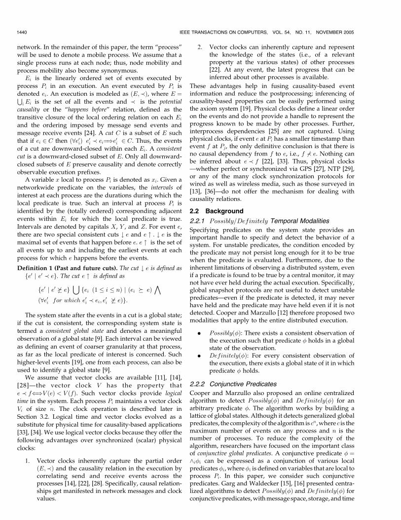
form a Boolean vector of length 12. Any two intervals at twoprocesses are related by one and only one interaction typeand no interaction type can be expressed in terms of theother interaction type—hence, the 29 interaction types forman orthogonal set of relations. Among these 29 interactions,there are 13 pairs of inverses and three are self-inverses. Forexample, IHðX;Y Þ is equivalent to IKðY ;XÞ as IH and IKare inverses of each other. Fig. 1 illustrates these interac-tions. Interval X is shown in a fixed position using a shadedrectangle, whereas multiple instances of interval Y , in-dicated using horizontal lines, are in different positionsrelative to X. minðXÞ and maxðXÞ denote the least andgreatest element of interval X, respectively. # minðXÞ,# maxðXÞ, minðXÞ " , and maxðXÞ " denote consistent cuts.The interaction type of each position of Y relative to X islabeled by IA through IX (and their modifiers). Fivepositions of Y have two labels each. The distinction betweenthe two interaction types represented in each of the fivepairs of labels arises due to the S1 and S2 relations and isshown at the right.

The nondense time model allows 11 interaction types

between a pair of intervals, defined in the lower part of

Table 3, in addition to the 29 identified above. There are five

pairs of inverses and one is its own inverse. These

interactions are illustrated in [19], which also explains the

significance of the nondense time model. The set of

40 orthogonal interaction types, also referred to interchang-

ably as modalities or relations, henceforth is denoted <.Examples of how the < modalities provide useful informa-

tion that is not provided by the Possibly=Definitely

classification are given in [20].

2.2.4 Modalities for Global Predicates

Observe that, for any predicate �, three orthogonal relational

possibilities hold under the Possibly/Definitely classification:

1 ) Definitelyð�Þ, 2 ) :Definitelyð�Þ ^ Possiblyð�Þ, 3 )

:Possiblyð�Þ. The 40 fine-grained orthogonal relational

possibilities in < have been mapped to the three orthogonal

relational possibilities based on the Possibly/Definitely classi-

fication (see [20]). Table 4 shows thismapping, assuming that

the conjunctivepredicate� isdefinedon twoprocesses.When

conjunctivepredicate� is definedover variables that are local

to n > 2 processes, one can still express the three possibilities

1) Definitelyð�Þ, 2 ) :Definitelyð�Þ ^ Possiblyð�Þ, and

3) :Possiblyð�Þ, in terms of the fine-grained 40 independent

relations between Cn2 pairs of intervals. Not all

40Cn2 combinations will be valid—the combinations have to

satisfy the axiom system given in [19].

Theorem 1 [20]. Consider a conjunctive predicate � ¼ ^i�i. The

following results are implicitly qualified over a set of intervals,

containing one interval per process:

. Definitelyð�Þ holds if and only ifV

ð8i2NÞð8j2NÞ½Definitelyð�i ^ �jÞ�.

. :Definitelyð�Þ ^ Possiblyð�Þ holds if and only if

ð9i 2 NÞð9j 2 NÞ:Definitelyð�i ^ �jÞ^

^ð8i2NÞð8j2NÞ

½Possiblyð�i ^ �jÞ�

0@

1A:

. :Possiblyð�Þ holds if and only if

ð9i 2 NÞð9j 2 NÞ:Possiblyð�i ^ �jÞ:

Example. Let � be ai ¼ 8 ^ bj ¼ 7 ^ ck ¼ 2. Let ai, bj, and

ck be 8, 7, 2, respectively, in intervals Xi, Yj, and Zk,

respectively, and let ICðXi; YjÞ, IRðYj; ZkÞ, and

IHðZk;XiÞ be true. See Fig. 2. Then, by Theorem 1,

w e h a v e 1 ) :Definitelyðai ¼ 8 ^ bj ¼ 7Þ a n d

Possiblyðai ¼ 8 ^ bj ¼ 7Þ, 2) :Definitelyðbj ¼ 7 ^ ck ¼ 2Þand Possiblyðbj ¼ 7 ^ ck ¼ 2Þ, and 3) :Definitelyðai ¼8 ^ ck ¼ 2Þ and Possiblyðai ¼ 8 ^ ck ¼ 2Þ. By Theorem 1,

we have the modality Possiblyð�Þ ^ :Definitelyð�Þ.Conversely, if Possiblyð�Þ ^ :Definitelyð�Þ is known in

the classical course-grained classification, the fine-

grained classification gives the added information:

ICðXi; YjÞ, IRðYj; ZkÞ, and IHðZk;XiÞ.


Fig. 1. Illustration of interaction types between intervals under the dense time model [19].

3 FRAMEWORK AND DATA STRUCTURES

3.1 Framework

Given a conjunctive predicate, for each pair of intervalsbelonging to different processes, each of the 29 (40) possibleindependent relations in the dense (nondense) model oftime can be tested for using the bit-patterns for thedependent relations, as given in Table 3. The tests for therelations R1, R2, R3, R4, S1, and S2 are given in the thirdcolumn of Table 2 using vector timestamps [14], [28]. Recallthat the interval at a process is used to identify the periodwhen some local property (using which the predicate � isdefined) holds. V �

i and V þi denote the vector timestamps at

process Pi at the start of an interval and the end of aninterval, respectively. V x

i denotes the vector timestamp ofevent xi at Pi. Observe from Table 2 that, to test for R1, R2,R3, and R4, an overhead of Oð1Þ time complexity is neededif the timestamps of the start and the end of the intervals areknown. However, for relations S1 and S2, if the tests areapplied in a naive manner, then it is also necessary to knowabout all the events in each interval.

Processes P1; P2; . . . ; Pn need to identify appropriate data,such as the timestamps of the start and end events of theirlocal intervals and timestamps of other communicationevents within the intervals, to track locally. This informationcan be sent using the network asynchronously and withoutany timing requirements to a central data fusion server P0.The only requirement is that, between any process and thedata fusion server, the logical link must be FIFO. The datafusion server maintains queues Q1; Q2; . . . ; Qn for intervalinformation from each of the processes. The server P0 itselfmay be a more powerful computing device than the typicalnodes deployed in the field. For each of the problems to besolved, the server runs an appropriately devised algorithmto process the interval information it receives in the queues.The algorithm logic has to detect “concurrent” pairwiseinteractions for each pair of intervals, considering only oneinterval from each process at a time as being a part of a

potential solution. A challenge to solving Fine Rel is to

formulate the necessary and sufficient conditions to

determine when to eliminate the received information

about intervals from the queues in order to process the

queues efficiently. These conditions are critical because

intervals that have been determined as not forming part of a

solution should get deleted from the queues at P0 so that

they are not considered in testing with other intervals.

Efficient data structures also need to be identified carefully.

It is important that the online algorithm has very low

message, space, and time complexity, particularly keeping

in mind the requirements of mobile networks—low power

availability and low bandwidth utilization.For Fine Poss and Fine Def , a critical new challenge is

to formulate different necessary and sufficient conditions

(than for Fine Rel) to determine when to eliminate

information about the intervals in the queues at P0. This is

because the deletion of the interval information cannot be

done based on the examination of whether a single relation

ri;j is satisfied for processes ðPi; PjÞ, as will be shown in

Section 5.We assume that interval X occurs at Pi and interval Y

occurs at Pj. For any two intervalsX andX0 that occur at the

same process, ifR1ðX;X0Þ, then we say thatX is a predecessor

ofX0 andX0 is a successor ofX. Also, there are amaximumof p

intervals at any process. The operations and data structures

required by the algorithms to solve Problems Fine Rel,

Fine Poss, Fine Def , and All Pairs Fine Rel can be

divided into two parts. The first part, common to all the

algorithms, runs on each of the n processes P1 to Pn and is

given in this section. The second part of each algorithm runs

on the data fusion process P0 and is presented in later

sections.

3.2 Clock and Log Operations

Each process Pi, where 1 � i � n, maintains the following

data structures:

. Vi : array ½1::n� of integer. This is the vector clock.

. Ii : array ½1::n� of integer. This is an Interval Clock,which tracks the latest intervals at processes. Ii½j� isthe timestamp Vj½j� when �j last became true.


Fig. 2. Example to show fine-grained relations across n ¼ 3 processes.

TABLE 4Refinement Mapping [20]

The upper part shows the 29 mappings under the dense time model.Under the nondense time model, the 11 additional mappings in the lowerpart also apply.

. Logi: Contains the information to be sent to thecentral process.

Fig. 3 shows how to maintain the vector clock (Rules 1-3)[14], [28] and the Interval Clock (Rules 2, 4, 5) proposed inthis paper. To maintain Logi, the required data structuresand operations are defined in Fig. 4. Logi is constructed andsent to the central process using the protocol shown. Thecentral process uses the Logs received to determine therelationship between two intervals.

3.3 Complexity Analysis at Pi ð1 � i � nÞTheorem 2. The average space complexity at Pi ð1 � i � nÞ is

6n� 2 integers.

Proof. Consider the construction algorithm for Log (Fig. 4).Each Log stores the start (V �) and the end (V þ) of aninterval, which requires 2n integers. Furthermore, anEvent_Interval is added to the Log for every component ofInterval Clock which is modified due to the receive of amessage. As a change in a component of Interval Clock

implies the start of a new interval on another process, thetotal number of times the component of Interval Clock

can change is equal to the number of intervals on all the

processes. Thus, the total number of Event Interval

which can be added to the Logs of a single process is

ðn� 1Þp. This takes 2ðn� 1Þp integers per process. Thus,

the total space for a single Log at a process can be up to

2nþ 2ðn� 1Þp. However, the total space needed for Logs

corresponding to all p intervals on a single process is

2ðn� 1Þpþ 2np. This gives an average of 4n� 2 integers

per Log at a process. As only one Log exists at a time, the

average space requirement at a process Pi ð1 � i � nÞ atany time is the sum of space required by vector clock,

Interval Clock, and Log, which is 6n� 2 integers. tuTheorem 3 (Message complexity).

. The total number of messages sent by the processes toP0 is Oðminðnp; 2ms þ 2mrÞÞ.

. The total message space overhead isOðminð4n2p� 2np; ð6ms þ 4mrÞnÞÞ.

Proof. The message complexity can be determined in two

ways:

1. As one message is sent per interval, the number ofmessages is OðpÞ for each Pi ði 6¼ 0Þ. This gives a


Fig. 3. The vector clock and the Interval Clock.

Fig. 4. Data structures and operations to construct Log at Pi (1 � i � n).

total message complexity of OðnpÞ. On average,the size of each message is 4n� 2 as each messagecontains the Log. The total message space over-head for a particular process is the sum of all theLogs for that process, which was shown to be4np� 2p. Hence, the total message space com-plexity is 4n2p� 2np ¼ Oðn2pÞ.

2. An optimization of message size can be used. TheLog corresponding to an interval is sent to thecentral process only if the relationship betweenthe interval and all other intervals (at otherprocesses) is different from the relationship whichits predecessor interval had with all the otherintervals (at other processes). Two successiveintervals, Y and Y 0, on process Pj will have thesame relationship if no message is sent orreceived by Pj between the start of Y and theend of Y 0. For each message exchanged betweenprocesses, a maximum of four interval Logs needto be sent to the central process because twosuccessive intervals (Y and Y 0) will have differentrelationships if a receive or a send occurs betweenthe start of Y and end of Y 0. This makes itnecessary to send two interval Logs for a sendevent and two for a receive event. Hence, if thereare ms number of send events and mr number ofreceive events in the execution (ms ¼ mr forunicasts), then a total of 2ms þ 2mr intervalsneeds to be sent to the central process in 2ms þ2mr control messages, while the total messagespace overhead is bounded by

2ms:nþ ð2ms þ 2mrÞ:2n ¼ 6msnþ 4mrn:

The first term, 2ms:n, arises because, for every

message sent, each other process eventually (due

to transitive propagation of Interval Clock) may

need to insert an Event Interval tuple in its Log.

This can generate an upper bound of 2nms

overhead in Logs across the n processes. Thesecond term, ð2ms þ 2mrÞ:2n, arises because the

vector clock at the start and end of each interval is

sent with each of the 2nms þ 2nmr control

messages.

Hence, the total number of control messages sent toP0 and the total message space overhead is the lesserof when either all the intervals are sent or when fourintervals are sent for each message exchanged. Thus,the total number of messages sent is Oðminðnp; 2ms þ2mrÞÞ and the total message space overhead isOðminð4n2p� 2np; ð6ms þ 4mrÞnÞÞ. tu

4 ALGORITHM Fine Rel(FINE-GRAINED RELATIONS)

To solve Problems Fine_Poss and Fine_Def, we first solve the

intermediate problem Fine_Rel, which was defined in

Section 1. Recall that the given relations fri;j; 8i; jg must

satisfy the axioms on< [19] for a solution to potentially exist.Algorithm Overview. The algorithm detects a set of

intervals, one on each process, such that each pair of

intervals satisfies the relationship specified for that pair ofprocesses. If no such set of intervals exists, the algorithmdoes not return any interval set. The central process P0

maintains n queues, one for Logs from each process, anddetermines which orthogonal relation holds between pairsof intervals. The queues are processed using “pruning,”described below. If there exists an interval at the head ofeach queue and these intervals cannot be pruned, then theseintervals satisfy ri;j 8 i; j, where i 6¼ j and 1 � i; j � n, and,hence, these intervals form a solution set.

The notion of pruning is developed by first defining theprohibition function and the allows relation.

Definition 2 (Prohibition function). Function H : < ! 2< isdefined to be Hðri;jÞ ¼ fR 2 < j R 6¼ ri;j ^ if RðX;Y Þ is

true then ri;jðX;Y 0Þ is false for all Y 0 that succeed Y g.

Intuitively, for each ri;j 2 <, the prohibition functionHðri;jÞ is the set of all orthogonal relations R ( 6¼ ri;j) suchthat if RðX;Y Þ is true, then ri;jðX;Y 0Þ can never be true forany successor Y 0 of Y . Hðri;jÞ is the set of relations thatprohibit ri;j from being true in the future.

Two relations, R0 and R00 (where R0 6¼ R00), in < arerelated by the allows relatione> if the occurrence of R0ðX;Y Þdoes not prohibit R00ðX;Y 0Þ for some successor Y 0 of Y .

Definition 3 (“allows” relation). e> is a relation on < � <such that R0e> R00 if 1) R0 6¼ R00 and 2) if R0ðX;Y Þ is true,then R00ðX;Y 0Þ can be true for some Y 0 that succeeds Y .

Example. ICe> IB because 1) IC 6¼ IB and 2) if ICðX;Y Þ istrue, then there is a possibility that IBðX;Y 0Þ is also true,where Y 0 succeeds Y .

Lemma 1. For R 6¼ ri;j, if R 2 Hðri;jÞ, then R 6e> ri;j, else if

R 62 Hðri;jÞ, then Re> ri;j.Proof. If R 2 Hðri;jÞ, using Definition 2, it can be inferred

that if RðX;Y Þ is true, then ri;j is false for all Y 0 thatsucceed Y . This does not satisfy the second part ofDefinition 3. Hence, R 6e> ri;j. If R 62 Hðri;jÞ and R 6¼ ri;j, itfollows that if RðX;Y Þ is true, then ri;jðX;Y 0Þ can be truefor some Y 0 that succeeds Y . This satisfies Definition 3and, hence, Re> ri;j. tu

Table 5 givesHðri;jÞ for each of the 40 interaction types in<. The table is constructed by analyzing each interactionpair in <.Example. The third row gives Hðri;jÞ for IC and IV . From

the second column,

HðICi;jÞðXi; YjÞ ¼ fIA; IB; IF; II; IP ; IO; IUX; IOPg:

Hence, for instance, if IBðXi; YjÞ, then ICðXi; Y0j Þ will

never hold for any successor Y 0j of Yj. From the third

column, HðIVi;jÞðXi; YjÞ ¼ < n fIQ; IV g. Hence, for in-stance, if IHðXi; YjÞ, then IV ðXi; Y

0j Þ will never hold for

any successor Y 0j of Yj.

We now state an important result between any tworelations in < that satisfy the “allows” relation and theexistence of the “allows” relation between their respectiveinverses. Specifically, if R0 allows R00, then Theorem 4 statesthat R0�1 necessarily does not allow relation R00�1. The


theorem can be observed to be true from Lemma 1 and

Table 5 by a case-by-case analysis.

Theorem 4. For R0; R00 2 <, if R0e> R00, then R0�1 6e> R00�1.

Example. ICe> IB ) IV ð¼ IC�1Þ 6e> IRð¼ IB�1Þ, which is

true. Note that R0 6¼ R00 in the definition of relation e> is

necessary; otherwise, R0e> R0 will become true and, from

Theorem 4, we get R0�1 6e> R0�1, which leads to a

contradiction.

Lemma 2. If the relationship RðX;Y Þ between intervals X and

Y (at processes Pi and Pj, respectively) is contained in the set

Hðri;jÞ, then interval X can be removed from the queue Qi.

Proof. From the definition of Hðri;jÞ, we get that ri;jðX;Y 0Þcannot exist, where Y 0 is any successor interval of Y .

Hence, interval X can never be a part of the solution and

can be deleted from the queue. tuLemma 3. If the relationship between a pair of intervals X and Y

(at processes Pi and Pj, respectively) is not equal to ri;j, then

either interval X or interval Y can be removed from the queue

Qi or Qj, respectively.

Proof. We use contradiction. Assume relation RðX;Y Þ( 6¼ ri;jðX;Y Þ) is true for intervals X and Y . From

Lemma 2, the only time neither X nor Y will be deleted

is when R 62 Hðri;jÞ and R�1 62 Hðrj;iÞ. From Lemma 1, it

can be inferred that R e> ri;j and R�1e> rj;i. As r�1i;j ¼ rj;i,

we get R e> ri;j and R�1e> r�1i;j . This is a contradiction as,

by Theorem 4, Re> ri;j ) R�1 6e> r�1i;j . Hence, R 2 Hðri;jÞ

or R�1 2 Hðrj;iÞ or both and, thus, at least one of the

intervals can be deleted. tu

Observe from Table 5 that it is possible that bothintervals being compared can be deleted.

Example. If ri;j ¼ IB is to be detected and it is determinedthat RðXi; YjÞ holds, where

RðXi; YjÞ 2 fIF ; II; IP ; IO; IU; IX; IUX; IOPg � Hðri;jÞ;

then Xi should be deleted. Also, we have that

R�1ðYj;XiÞ 2fIF�1; IP�1; IO�1; IU�1; IX�1; IUX�1; IOP�1g � Hðrj;iÞ

and, hence, Yj should also be deleted. This can also beseen from Fig. 1.

Theorem 5. Algorithm Fine_Rel run by P0 in Fig. 6 solvesProblem Fine_Rel.

Proof sketch. Lemma 2, which allows queues to be prunedcorrectly, is implemented in the algorithm at P0. Thecode shown is executed atomically when an intervalarrives at P0. The orthogonal interaction RðX;Y Þbetween a pair of intervals X and Y being consideredis determined in line 12. This determination is done byevaluating R1 to R4 using the tests in Table 2 and byevaluating S1 and S2 using the tests in Fig. 5 thatimplement their definitions in Table 2. Using thisinformation, the bit-vector in Table 3 identifies theorthogonal interaction type between X and Y . Thealgorithm deletes interval X as soon as RðX;Y Þ 2Hðri;jÞ (lines 13-17). Similarly, Y is deleted if RðY ;XÞ 2Hðrj;iÞ (lines 15-17). Thus, an interval gets deleted only ifit cannot be part of the solution. Also, clearly, each


TABLE 5Hðri;jÞ for the 40 Independent Relations in <

The upper part of the table gives the functionH on 29 relations assuming dense time. The lower part of the table gives functionH for the 11 additionalrelations assuming nondense time.

interval gets processed unless a solution is found using a

predecessor interval from the same process. Lemma 3

gives the unique property that if RðX;Y Þ 6¼ ri;j, then

either interval X or interval Y is deleted. A consequence

of this property is that if every queue is nonempty and

their heads cannot be pruned, then a solution exists and

the set of intervals at the head of each queue forms a

solution.


Fig. 5. Tests for coupling relations S1ðX; Y Þ and S2ðY ;XÞ at P0. The tests implement the definitions given in Table 2.

Fig. 6. Online algorithm Fine Rel at the data fusion server P0.

The set updatedQueues stores the indices of all thequeues whose heads got updated. In each iteration of thewhile loop, the indices of all the queues whose headssatisfy Lemma 2 are stored in set newUpdatedQueues(lines 13-16). In lines 17 and 18, the heads of all thesequeues are deleted and indices of the updated queuesare stored in the set updatedQueues. Observe that onlyinterval pairs which were not compared earlier arecompared in subsequent iterations of thewhile loop. Theloop runs until no more queues can be updated. If, at thisstage, all the queues are nonempty, then a solution isfound (follows from Lemma 3). If a solution is found,then, for the intervals X (at Pi) and Y (at Pj) stored at theheads of these queues, we have RðX;Y Þ ¼ ri;j. tu

Theorem 6. Algorithm Fine Rel has the following complexities:

. The total space complexity at process P0 isOðminðð4n� 2Þnp; ð6ms þ 4mrÞnÞÞ.

. The average time complexity at P0 isOððn� 1Þminðð2ms þ 2mrÞ; pnÞÞ. This is equivalentto Oðn2MÞ, where M is maximum number of entriesin a queue.

Proof. For the central process P0, the total space required isOðminðð4n� 2Þnp; ð6ms þ 4mrÞnÞÞ because the totalspace overhead at P0 is equal to the total message spacecomplexity (see Theorem 3).

The time complexity is the product of the number ofsteps required to determine an orthogonal relationshipfrom < and the number of relationships determined.

Consider the first part of the product:

. The total number of interval pairs between anytwo processes Pi and Pj is p2. To determineR1ðX;Y Þ to R4ðX;Y Þ and R1ðY ;XÞ to R4ðY ;XÞ,as eight comparisons are needed for each intervalpair, 8p2 comparisons are necessary for any pairof processes.

. To determine the number of comparisons requiredby S1 and S2, consider the maximum number ofEvent Intervals stored in Logj:p log½i� that are sentover the execution lifetime to the central process aspart of the Logs. This is the maximum number ofEvent Intervals corresponding to Pi stored in Qj

over Pj’s execution lifetime. An Event Interval isadded to Logj:p log½i� only when there is a changein the ith component of Interval Clock at thereceive of a message. As the ith component ofInterval Clock changes only when a new intervalstarts, the total number of times the ith compo-nent of Interval Clock changes is at most equal top, the maximum number of intervals occurring onthe other process Pi. From Fig. 5, it can beobserved that, for each Event Interval, there isone comparison. Thus, to determine the relation-ship between an interval on Pj and all otherintervals on Pi, the number of comparisons isequal to p. As there are p intervals on Pj, a total ofp2 comparisons are required to determine S1 orS2. Hence, the total number of comparisons todetermine S1ðX;Y Þ, S2ðX;Y Þ, S1ðY ;XÞ, andS2ðY ;XÞ is 4p2.

This gives a total of 8p2 þ 4p2 ¼ Oðp2Þ comparisons todetermine the relation between each pair of intervals on apair of processes. As there are a total of p2 intervals pairsbetween two processes, the average number of compar-isons required to determine a relationship is Oð1Þ.

To analyze the second part of the product, considerFig. 6. For each interval considered from one of thequeues in updatedQueues (lines 6-12), the number ofrelations determined is n� 1. Thus, the number ofrelations determined for each iteration of the while loopis ðn� 1ÞjupdatedQueuesj, where jupdatedQueuesj de-notes the number of entries in updatedQueues. Thecumulative

PjupdatedQueuesj over all iterations of the

while loop is less than the total number of intervals overall the queues. Thus, the total number of relationsdetermined is less than ðn� 1Þminð2ms þ 2mr; pnÞ,where minð2ms þ 2mr; npÞ is the upper bound on thetotal number of intervals over all the queues. As theaverage time required to determine a relationship isOð1Þ, the average time complexity of the algorithm isequal to Oððn� 1Þminð2ms þ 2mr; pnÞÞ.

The average time complexity is equivalently ex-pressed using M, the maximum number of entries in aqueue, as follows: The total number of intervals over allthe queues is OðnMÞ. As the total number of relationsdetermined is ðn� 1Þ

PjupdatedQueuesj over all the

iterations of the while loop, this is equivalent toðn� 1Þ:nM ¼ Oðn2MÞ. This is also the average timecomplexity as it takes Oð1Þ time on average to determinea relationship. tu

Table 1 compares the complexities of Fine Rel withthose of earlier algorithms [15], [16] to detect Possibly andDefinitely. The earlier algorithms computed their timecomplexity at P0 as Oðn2MÞ, not in terms of ms, mr, or p.They did not give the space complexity at P0. As eachcontrol message in these earlier algorithms carries a fixedsize OðnÞmessage overhead and a control message is sent toP0 for every message send/receive event, we computedtheir total space complexity and average time complexity atP0 as OðnmrÞ. This enables a direct comparison with the ouralgorithm. Further, we have also computed our averagetime complexity, using M, as Oðn2MÞ. In our algorithm,note that M � p; M ¼ p if the message overhead optimiza-tion is not used. We do not express the total space at P0 interms of M because the queue entries are of variable size,with an average size of ð4n� 2Þ integers.

5 ALGORITHMS Fine Poss AND Fine Def

By leveraging Theorem 1 and the mapping of fine-grainedmodalities to Possibly and Definitely modalities, as givenin Table 4, we address the problems of determining whetherPossiblyð�Þ and Definitelyð�Þ hold. If either of these twocoarse-grained modalities holds, we can also determine theexact fine-grained orthogonal relation/modality betweeneach pair of processes, unlike any previous algorithm.Further, the time, space, and message complexities of theproposed online (centralized) detection algorithms (Algo-rithms Fine Poss and Fine Def) to detect Possibly and


Definitely in terms of the fine-grained modalities per pairof processes are the same as those of the earlier online(centralized) algorithms [15], [16] that can detect onlywhether the Possibly and Definitely modalities hold.

Recall that< is a set of orthogonal relations and, hence, oneand only one relation from <must hold between any pair ofintervals. Consider the case where, for each pair of processesðPi; PjÞ, there is a set ri;j < such that some relation in ri;jmust hold. Now, consider the objective where we need toidentify one interval per process such that, for each processpair ðPi; PjÞ, some relation in ri;j holds for that ðPi; PjÞ. Weformalize this objective by generalizing the detection pro-blem Fine Rel to problem Fine Rel0, as follows:

Problem Fine Rel0 Statement. Given a set of relations ri;j <for each pair of processes Pi and Pj, determine online the

intervals, if they exist, one from each process, such that any

one of the relations in ri;j is satisfied (by the intervals) for each

(Pi; Pj) pair. If a solution exists, identify the fine-grained

interaction from < for each pair of processes.

To solve Fine Rel0, given an arbitrary ri;j, a solutionbased on Algorithm Fine Rel (Fig. 6) will not work because,in the crucial tests in lines 13-14, neither interval may beremovable and yet none of the relations from ri;j might holdbetween the two intervals. This leads to deadlock! To seethis further, let r1; r2 2 ri;j and let RðX;Y Þ hold, whereR 62 ri;j. Now, let R 2 Hðr1Þ, R�1 62 Hðr1�1Þ, R 62 Hðr2Þ,R�1 2 Hðr2�1Þ. Interval X cannot be deleted becauseR 62 Hðr2Þ, implying that r2ðX;Y 0Þ may be true for asuccessor Y 0 of Y . Interval Y cannot be deleted becauseR�1 62 Hðr1�1Þ, implying that r1�1ðY ;X0Þ may be true for asuccessor X0 of X. Therefore, a solution based on AlgorithmFine Rel will deadlock and a more elaborate (and pre-sumably more expensive) solution will be needed.

Example. Let ri;j ¼ fIB; IGg and let RðX;Y Þ ¼ IH. NeitherX nor Y can be deleted.

We now identify and define a special property, termedCONVEXIT Y, on ri;j such that the deadlock is prevented.Informally, this property says that there is no relation R

outside ri;j such that, for any r1; r2 2 ri;j, R e> r1 andR�1e> r2�1. This property guarantees that, when intervals Xand Y are compared for ri;j and RðX;Y Þ holds, either X orY or both get deleted and, hence, there is progress. The setsri;j, derived from Table 4, that need to be detected to solveProblems Fine_Poss and Fine_Def satisfy this property. Wetherefore observe that problems Fine_Poss and Fine_Def arespecial cases of Problem Fine Rel0 in which the propertyCONVEXIT Y on ri;j is necessarily satisfied. To solveProblems Fine Poss and Fine Def , we then use the

generalizations of Lemmas 2 and 3, as given in Lemmas 4and 5, respectively, to first solve Fine Rel0.

Definition 4 (Convexity).

CONVEXIT Y : 8R 62 ri;j :

8ri;j 2 ri;j; R 2 Hðri;jÞ_

8rj;i 2 rj;i; R�1 2 Hðrj;iÞ

� �:

Lemma 4. If the relationship RðX;Y Þ between intervals X and

Y (at processes Pi and Pj, respectively) is contained in the setTri;j2ri;j

Hðri;jÞ, then interval X can be removed from the

queue Qi.

Proof. From the definition of Hðri;jÞ, we infer that norelation ri;jðX;Y 0Þ, where ri;j 2 ri;j and Y 0 is anysuccessor interval of Y on Pj, can be true. Hence,interval X can never be a part of the solution and can bedeleted from the queue. tu

Lemma 5. If the relationship RðX;Y Þ between a pair of intervals

X and Y (at processes Pi and Pj, respectively) does not belong

to the set ri;j, where ri;j satisfies property CONVEXIT Y,then either intervalX or interval Y is removed from the queue.

Proof. We use contradiction. Assume relation RðX;Y Þ( 62 ri;jðX;Y Þ) is true for intervals X and Y . From

Lemma 4, the only time neither X nor Y will be deleted

is when bothR 62T

ri;j2ri;jHðri;jÞ andR�1 62

Trj;i2rj;i

Hðrj;iÞ.However, as ri;j satisfies property CONVEXIT Y, we

have that R 2T

ri;j2ri;jHðri;jÞ or R�1 2

Trj;i2rj;i

Hðrj;iÞmust

be true. Thus, at least one of the intervals can be deleted

by an application of Lemma 4. tuThe proof of the following theorem is similar to the proof

of Theorem 5.

Theorem 7. If the set ri;j satisfies property CONVEXIT Y, thenProblem Fine Rel0 is solved by replacing lines 13 and 15 in

Algorithm Fine Rel in Fig. 6 by lines 13 and 15 in Fig. 7.

Proof. Analogous to the proof of Theorem 5. Use Lemmas 4and 5 instead of Lemmas 2 and 3, respectively, andreason with ri;j instead of with ri;j. tu

Corollary 1. The time, space, and message complexities of

Algorithm Fine Rel0 are the same as those of Algorithm

Fine Rel, which were stated in Theorem 6.

Proof. The only changes to Algorithm Fine Rel are in

lines 13 and 15. In Algorithm Fine Rel0, instead of

checking RðX;Y Þ for membership in Hðri;jÞ in line 13,

RðX;Y Þ is checked for membership inT

ri;j2ri;jHðri;jÞ.

Both Hðri;jÞ andT

ri;j2ri;jHðri;jÞ are sets of size between 0


Fig. 7. Algorithm Fine Rel0: Changes to Algorithm Fine Rel are listed, assuming ri;j satisfies Property CONVEXIT Y.

and j<j ¼ 40. An analogous observation holds for the

change on line 15. Hence, the time, space, and message

complexities of Fine Rel are unaffected in Fine Rel0. tuTo detect Possiblyð�Þ, ri;j is set to the union of the

orthogonal interactions in the first two columns of Table 4.We can verify (by case-by-case enumeration) that ri;j doessatisfy Property CONVEXIT Y. Similarly, to detectDefinitelyð�Þ, ri;j is set to the union of the orthogonalinteractions in the first column of Table 4. We can verify (bycase-by-case enumeration) that ri;j does satisfy PropertyCONVEXIT Y.

The following two theorems about using algorithmFine Rel0 (Fig. 7) to solve Problems Fine Poss andFine Def can be readily proven by using Theorem 1, therefinement mapping of Table 4, and Theorem 7. The tworesulting algorithms are named Fine Poss and Fine Def ,respectively.

Theorem 8. Algorithm Fine Rel modified to AlgorithmFine Rel0 (Fig. 7) solves Problem Fine Poss (aboutPossiblyð�Þ) when ri;j is set to the union of the relations inthe first and second columns of Table 4.

Proof. From Theorem 1, Possiblyð�Þ is true if and only ifð8i 2 NÞð8j 2 NÞPossiblyð�i ^ �jÞ. For any i and j,Possiblyð�i ^ �jÞ is true if and only if RðXi; YjÞ is anyof the temporal relations given in the first two columnsof Table 4. When ri;j is set to the union of the relations inthese two columns, we can verify (by case-by-caseenumeration) that ri;j satisfies CONVEXIT Y. As Algo-rithm Fine Rel0 is correct (by Theorem 7), when its ri;j isinstantiated with the set above to get AlgorithmFine Poss, we have that Fine Poss is also correct. tu

Theorem 9. Algorithm Fine Rel modified to AlgorithmFine Rel0 (Fig. 7) solves Problem Fine Def (aboutDefinitelyð�Þ) when ri;j is set to the union of the relationsin the first column of Table 4.

Proof. From Theorem 1, Definitelyð�Þ is true if and only ifð8i 2 NÞð8j 2 NÞDefinitelyð�i ^ �jÞ. For any i and j,Definitelyð�i ^ �jÞ is true if and only if RðXi; YjÞ is anyof the temporal relations given in the first column ofTable 4. When ri;j is set to the relations in this column,we can verify (by case-by-case enumeration) that ri;jsatisfies CONVEXIT Y. As Algorithm Fine Rel0 iscorrect (by Theorem 7), when its ri;j is instantiated withthe set above to get Algorithm Fine Def , we have thatFine Def is also correct. tu

In Algorithm Fine Rel0, when ri;j is set to the values

as specified in Theorems 8 and 9 to detect Possibly

and Definitely, respectively, the setT

ri;j2ri;jHðri;jÞ used

in line 13 of the algorithm becomes fIAg and

fIA; IB; IC; IG; IH; II; IK; IV ; IM 00; IMN 00; IMNg, respec-tively. An identical change occurs to the set

Trj;i2rj;i

Hðrj;iÞon line 15.

Corollary 2. The time, space, and message complexities ofAlgorithms Fine Poss and Fine Def are the same as thoseof Algorithm Fine Rel (stated in Theorem 6) and ofAlgorithm Fine Rel0 (stated in Corollary 1).

Proof. Follows from Corollary 1 and the fact that ri;j forFine Poss and Fine Def satisfy CONVEXIT Y and areinstantiations of ri;j in Fine Rel0. tu

6 ALGORITHM All Pairs Fine Rel

Using the tests in Table 2 and Fig. 5, we can determine the 12-bit pattern of Table 3 and, hence, the interaction type betweena pair of intervals. To determine the relations between allpairs of intervals fromdifferent processes, the total number ofintervals stored at P0 across all the queues Q1 to Qn in theworst case is pn. The number of runs of the tests required todetermine the relationbetweenall pairs of intervals is equal tothe total number of pairs of intervals, which is Cn

2 :p2. To

reduce the memory overhead and the number of tests, thefollowing queue pruning scheme is used.

Lemma 6. If the relation R between an interval X and intervalY is contained in the set S ¼ fr 2 < j rðX;Y Þ )R2ðX;Y Þ ¼ 1 (defined in Table 3) g ¼ fIA; IB; II; IX; IO;IP; IF ; IU; IUX; IOPg, then X and the successors ofinterval Y being queued on Qj are related by IA and nofurther comparison is needed between them.

Proof. As the control messages from any process arereceived by P0 in FIFO order, the interval Y 0 that getsqueued after Y in Qj is a successor of Y . This, coupledwith the fact that RðX;Y Þ 2 S, implies V þ

i ðXÞ is less thanV þj ðY Þ, which in turn implies V �

j ðY 0Þ is greater thanV þi ðXÞ. Thus, the only relation possible between X and

Y 0 is IA. tu

Using Lemma 6, we can reduce the number ofcomparisons.

Lemma 7. If Lemma 6 is satisfied for an interval X with respectto at least one interval on each of the other queues, theninterval X can be removed from its queue.

Proof. As Lemma 6 is satisfied for interval X with respect toat least one interval Yj on each other queue Qj, weconclude that RðX;Y 0

j Þ ¼ IA between X and anysubsequent interval Y 0

j after Yj on Qj. Hence, we canremove X from its queue. tu

The above lemma is used to decrease the memorystorage overhead for the central process P0. Both of theabove lemmas are used in the predicate detection algorithmat P0. Fig. 8 gives an efficient algorithm to detect therelationship between each pair of intervals.

Theorem 10. The algorithm run by P0 in Fig. 8 solves ProblemAll Pairs Fine Rel.

Proof sketch. An interval X received at P0 is enqueued inQi and compared with intervals on all the other queues.The algorithm stops comparison of interval X withsuccessors of interval Y as soon as X and Y satisfyLemma 6. The interval X is pruned from the queue afterit satisfies Lemma 7, i.e., it satisfies Lemma 6 with respectto all the processes. This is determined by keeping ann-bit array B for each of the intervals stored in thequeues at process P0. For interval X on queue Qi, then-bit array is represented by BX

i . If BXi ½j� is set to 1 when

comparing intervals X and Y (lines 8-9), then no


comparison is needed between X and any successor of Y

because the relationship between X and successors of Y

will be IA. Thus, the relation between all interval pairs is

explicitly determined except when it is known to be IA

or IQ. tuTheorem 11. Algorithm All Pairs Fine Rel has the following

complexities:

. The total message space complexity is Oðn2pÞ.

. The total space complexity at process P0 is Oðn2pÞ.

. The average time complexity at P0 is Oðn2p2Þ.Proof. The total message space complexity can be shown as in

Theorem 3 to be Oðn2pÞ. The message optimization used

there is not applicable as all intervals need to be

considered in All_Pairs_Fine_Rel.The space complexity at P0 is the space occupied by all

the queues. This includes the total message spacecomplexity and also the OðnÞ space for each of the npinstances of the B array. The space complexity at P0 isthus Oðn2pÞ.

The time complexity is the product of the number ofsteps required to determine a relationship from < andthe number of relationships determined.

. It was shown in the proof of Theorem 6 that 1) atotal of Oðp2Þ comparisons are needed to deter-mine a relationship between each pair of intervalson a given pair of processes and 2) it takesaverage time Oð1Þ to determine a relationship.

. There are Cn2 or Oðn2Þ pairs of processes.

Hence, the average time complexity of the algorithm is

Oðn2p2Þ. The actual time complexity is expected to be

much less as the number of comparisons may be greatly

reduced by using Lemmas 6 and 7. tu

7 OPERATION IN MOBILE SYSTEMS

The complexity of the algorithms to solve Fine Rel,

Fine Poss, and Fine Def is shown in Table 1. It can be

seen that these algorithms have low overhead. All the

measures at P0 are either linear or quadratic in n, the size of

the mobile ad hoc network. This indicates high scalability of

the algorithms. Most importantly, the size of the space

requirement at each process Pi (i 2 ½1; n�), which is bothspace and energy constrained, is linear in n. This makes the

algorithm easily implementable and scalable.Recall that mobility is implicitly permitted in the model

(Section 2.1). We now show how to implement the

algorithms in mobile ad hoc networks. The algorithms

require each process Pi (1 � i � n) to eventually and

asynchronously (via any routes) send its event stream to a

central data fusion server process P0 via a FIFO channel,

which can be achieved in mobile ad hoc networks. We use

hierarchical clustering to manage the network. Further

scalability can be achieved by using “hierarchical” time-stamps based on logical clocks. Several efficient implemen-

tations of vector clocks, such as the difference method [35]

and others surveyed in [22], can also be used in conjunction.In the hierarchical organization of the clusters, the data

fusion server P0 is the root and a logical tree is super-

imposed such that the mobile processes are the leaf nodes.

Communication paths from the leaves to the root can be

provided by the hierarchical mobile routing algorithms [2],

[3], [4], [26], [30], [32]. The FIFO channels between each Pi

(i 6¼ 0) and P0 can also be implemented using sequence

numbering with retransmissions at the application layer,rather than in the MAC layer. For a kþ 1 level hierarchy,

each cluster at each level except the highest level can be

organized to have approximately � nodes, where n ¼ �k.

The above algorithms [2], [3], [4], [26], [30], [32] can be used

to maintain the hierarchical cluster organization despite

mobility and failures. For example, for greater fault

tolerance (to node failures), there can be some overlap

among the clusters [3]. In particular, the following can be

ensured using these algorithms:

. Despite mobility of the processes, the hierarchicaltree structure is maintained. Thus, some clusterheadis always identified with each node, using handoff.

. Despite mobility, occasional lost connectivity, andnode deaths, a FIFO logical channel is maintainedbetween each Pi (1 � i � n) and P0.

. If a node dies, the algorithm at P0 is not blocked. If anode in the hierarchy dies, the subtree rooted at thatnode gets reconnected.


Fig. 8. Algorithm All Pairs Fine Rel: to determine the relations between each pair of intervals.

. The algorithm works seamlessly and correctly withbackup data fusion server(s), in case of serverfailure. Event stream routing transparently flipsover to the backup server while maintaining theFIFO property from each node to the server.

The algorithms proposed in this paper used online,

centralized fusion of the data collected from distributed

processes. Although completely distributed and symme-

trical algorithms performing distributed data fusion can be

designed, they are not inherently suitable for mobile ad hoc

networks.

1. The full symmetry may replicate the data fusionwork at all the mobile nodes.

2. Decision-making often requires extra “meta-infor-mation” after the fusion, and such meta-informationis best kept at some server P0 (with a few backupreplicas for fault tolerance). Mobile nodes may notbe capable of decision making and a known logicallocation for decision making is preferred.

3. Fully symmetrical algorithms tend to place higheroverhead on all the participants, in terms of some/all of space, time, and message complexity.

4. A distributed algorithm requires communicationbetween any pair of processes, thus requiring a moreelaborate routing scheme (any-to-any) and not justbetween the leaves and the root. (Multicasting as in[10] may be used for the distributed algorithm, butmulticast overheads would be incurred.)

8 CONCLUSIONS AND DISCUSSION

This paper proposed online algorithms for detecting

conjunctive predicates and behavioral patterns that can be

specified using a rich palette of fine-grained temporal mod-

alities. Algorithm Fine Rel solves a fundamental problem of

identifying a global state satisfying fine-grained interaction

modalities between each pair of processes. Algorithms

Fine Poss and Fine Def not only detect Possiblyð�Þ and

Definitelyð�Þ, respectively, but also (unlike previous algo-

rithms) return the pairwise fine-grained relations which

exist between all the intervals in the solution set. The space,

message and computational complexities of the previous

works for conjunctive predicate detection, which can detect

only Possiblyð�Þ [15] or only Definitelyð�Þ [16], are

compared with our algorithms in Table 1. All the complex-

ity measures for algorithms Fine Poss and Fine Def are

the same as those for the algorithms [15] and [16],

respectively. Thus, with the same overhead, algorithms

Fine Poss and Fine Def do the extra work of finding the

fine-grained relations which exist between the intervals

contained in the solution set for Possibly and Definitely.

The output of All_Pairs_Fine_Rel can be used to mine

patterns in the execution.The space, communication, and time overheads of the

algorithms are low, making them deployable in resource-

constrained mobile ad hoc networks. The algorithms are

highly scalable in that the space requirement at each mobile

node is of the order of the size of the system. We showed

how to run the algorithms in a mobile ad hoc network.

Two distributed algorithms have been proposed for

F in e_Re l . The f i r s t a lgo r i thm [5 ] , [ 6 ] u se s

Oðnminðnp; 4mnÞÞ messages of size OðnÞ each (here, m

is the maximum number of messages sent by any

process). The second algorithm [6], [17] uses

Oðminðnp; 4mnÞÞ messages of size Oðn2Þ each. For both

the algorithms, the total space complexity across all the

processes is minð4n2p� 2np; 10n2mÞ, the worst-case space

overhead per process is minð4np� 2p; 4mn2 þ 2mn� 2mÞ,and the time complexity at a process is Oðminðnp; 4mnÞÞ.Analogous to the approach in this paper, the distributed

algorithms can be used to design distributed versions of

Fine Poss and Fine Def .Alternate definitions [17] of e> and H that exclude the

condition R 6¼ ri;j lead to a simpler structure of the allows

relation. The formalism will need to change accordingly.

For example, the condition on lines 13 and 15 in Fig. 6

would also require RðX;Y Þ 6¼ ri;j and RðY ;XÞ 6¼ rj;i,

respectively, to be true. As another example, the condition

on lines 13 and 15 in Fig. 7 would also require RðX;Y Þ 62 ri;jand RðY ;XÞ 62 rj;i, respectively, to be true.

A discussion of how the presented algorithms andapproach can be used to detect nonconjunctive predicates,i.e., general relational predicates, is given in [21]. The keyidea is to compose and redefine “intervals” at the datafusion server using the execution’s state lattice.

The proposed algorithms assume that the processes can

timestamp (using vector clocks) the events within the

executions of the processes. Recent advances in cost-

effective technology have led to a spurt in designing sensor

networks and actuator networks [1], [31], [37], [38] to

observe real-world physical phenomena. Such networks

typically use synchronized physical clocks; [36] surveys

physical clock synchronization schemes for wireless sensor

networks. Events in the environment are outside of the

processes. Causality-based properties could be detected if

the sensors can 1) detect communication within the physical

environment being sensed (outside the network) and

2) assign logical vector timestamps to the communication

events and events in the environment at which the

monitored variables change. Thus, if it were possible to

manifest causal relations in the events and communication

within the environment, each sensed location can be

assigned a “time-line” be modeled as another “process,”

and be included in the causality analysis. It does not seem

that this can be done.Recent results on detecting predicates that are specified

using physically synchronized clocks are presented in [23].

ACKNOWLEDGMENTS

An earlier version of some portions of this paper appeared

in the Proceedings of the 2003 ASIAN Computing Science

Conference [8].

REFERENCES

[1] I. Akyildiz, W. Su, Y. Sankarasubramanian, and E. Cayirci,“Wireless Sensor Networks: A Survey,” Computer Networks,vol. 38, no. 4, pp. 393-422, 2002.


[2] A. Amis, R. Prakash, T. Vuong, and D. Huynh, “Max-MinD-Cluster Formation in Wireless Ad-Hoc Networks,” Proc. IEEEInfocom, pp. 32-41, 2000.

[3] S. Banerjee and S. Khuller, “A Clustering Scheme for HierarchicalControl in Multi-Hop Wireless Networks,” Proc. IEEE Infocom,pp. 1028-1037, Apr. 2001.

[4] D. Baker and A. Ephremedis, “The Architectural Organization of aMobile Radio Network via a Distributed Algorithm,” IEEE Trans.Comm., vol. 29, pp. 1694-1701, Nov. 1981.

[5] P. Chandra and A.D. Kshemkalyani, “Detection of OrthogonalInterval Relations,” Proc. Ninth Int’l Conf. High-PerformanceComputing, pp. 323-333, 2002.

[6] P. Chandra and A.D. Kshemkalyani, “Distributed Detection ofTemporal Interval Interactions,” Technical Report UIC-ECE-02-07,Univ. of Illinois at Chicago, Apr. 2002.

[7] P. Chandra and A.D. Kshemkalyani, “Distributed Algorithm toDetect Strong Conjunctive Predicates,” Information ProcessingLetters, vol. 87, no. 5, pp. 243-249, Sept. 2003.

[8] P. Chandra and A.D. Kshemkalyani, “Global Predicate Detectionunder Fine-Grained Modalities,” Proc. ASIAN Computing ScienceConf. 2003, pp. 91-109, Dec. 2003.

[9] K.M. Chandy and L. Lamport, “Distributed Snapshots: Determin-ing Global States of Distributed Systems,” ACM Trans. ComputerSystems, vol. 3, no. 1, pp. 63-75, 1985.

[10] C.-C. Chiang, M. Gerla, and L. Zhang, “Tree Multicast Strategiesin Mobile, Multihop Wireless Networks,” Mobile Networks andApplications (MONET), vol. 3, pp. 193-207, 1999.

[11] G. Coulouris, J. Dollimore, and T. Kindberg, Distributed SystemsConcepts and Design, third ed. Addison-Wesley, 2001.

[12] R. Cooper and K. Marzullo, “Consistent Detection of GlobalPredicates,” Proc. ACM/ONR Workshop Parallel and DistributedDebugging, pp. 163-173, May 1991.

[13] J. Elson and K. Romer, “Wireless Sensor Networks: A NewRegime for Time Synchronization,” Proc. First Workshop Hot Topicsin Networks (HotNets-I), Oct. 2002.

[14] C.J. Fidge, “Timestamps in Message-Passing Systems that Pre-serve Partial Ordering,”Australian Computer Science Comm., vol. 10,no. 1, pp. 56-66, Feb. 1988.

[15] V.K. Garg and B. Waldecker, “Detection of Weak UnstablePredicates in Distributed Programs,” IEEE Trans. Parallel andDistributed Systems, vol. 5, no. 3, pp. 299-307, Mar. 1994.

[16] V.K. Garg and B. Waldecker, “Detection of Strong UnstablePredicates in Distributed Programs,” IEEE Trans. Parallel andDistributed Systems, vol. 7, no. 12, pp. 1323-1333, Dec. 1996.

[17] P. Chandra and A.D. Kshemkalyani, “Global State DetectionBased on Peer-to-Peer Interactions,” Proc. IFIP Int’l Conf. Embeddedand Ubiquitous Computing, Dec. 2005.

[18] M. Hurfin, M. Mizuno, M. Raynal, and M. Singhal, “EfficientDistributed Detection of Conjunctions of Local Predicates,” IEEETrans. Software Eng., vol. 24, no. 8, pp. 664-677, Aug. 1998.

[19] A.D. Kshemkalyani, “Temporal Interactions of Intervals inDistributed Systems,” J. Computer and System Sciences, vol. 52,no. 2, pp. 287-298, Apr. 1996.

[20] A.D. Kshemkalyani, “A Fine-Grained Modality Classification forGlobal Predicates,” IEEE Trans. Parallel and Distributed Systems,vol. 14, no. 8, pp. 807-816, Aug. 2003.

[21] A.D. Kshemkalyani, “A Note on Fine-Grained Modalities forNonconjunctive Predicates,” Proc. Fifth Int’l Workshop DistributedComputing, pp. 11-25, Dec. 2003.

[22] A.D. Kshemkalyani, “The Power of Logical Clock Abstractions,”Distributed Computing, vol. 17, no. 2, pp. 131-150, Aug. 2004.

[23] A.D. Kshemkalyani, “Predicate Detection Using Event Streams inUbiquitous Environments,” Proc. Int’l Symp. Network-CentricUbiquitous Systems, Dec. 2005.

[24] L. Lamport, “Time, Clocks, and the Ordering of Events in aDistributed System,” Comm. ACM, vol. 21, no. 7, pp. 558-565, July1978.

[25] L. Lamport, “On Interprocess Communication, Part I: BasicFormalism; Part II: Algorithms,” Distributed Computing, vol. 1,pp. 77-85, vol. 1, pp. 86-101, 1986.

[26] C.R. Lin and M. Gerla, “Adaptive Clustering for Mobile WirelessNetworks,” IEEE J. Selected Areas in Comm., vol. 15, no. 7, pp. 1265-1275, Sept. 1997.

[27] T. Logsdon, The Navstar Global Positioning System. New York: VanNostrand/Reinhold, 1992.

[28] F. Mattern, “Virtual Time and Global States of DistributedSystems,” Parallel and Distributed Algorithms, pp. 215-226, North-Holland, 1989.

[29] D. Mills, “Internet Time Synchronization: The Network TimeProtocol,” IEEE Trans. Comm., vol. 39, no. 10, pp. 1482-1493, Oct.1991.

[30] G. Pei, M. Gerla, X. Hong, and C. Chiang, “A WirelessHierarchical Routing Protocol with Group Mobility,” IEEEWireless Comm. and Networking Conference (WCNC), pp. 1538-1542, 1999.

[31] G. Pottie and W. Kaiser, “Wireless Integrated Network Sensors,”Comm. ACM, vol. 43, no. 5, pp. 51-58, May 2000.

[32] R. Ramanathan and M. Steenstrup, “Hierarchically Organized,Multihop Wireless Mobile Wireless Networks for Quality-Of-Service Support,” Mobile Networks and Applications (MONET),vol. 3, no. 1, pp. 101-110, June 1998.

[33] M. Raynal and M. Singhal, “Logical Time: Capturing Causality inDistributed Systems,” Computer, vol. 29, no. 2, pp. 49-56, Feb. 1996.

[34] R. Schwarz and F. Mattern, “Detecting Causal Relationships inDistributed Computations: In Search of the Holy Grail,” Dis-tributed Computing, vol. 7, pp. 149-174, 1994.

[35] M. Singhal and A.D. Kshemkalyani, “Efficient Implementation ofVector Clocks,” Information Processing Letters, vol. 43, pp. 47-52,Aug. 1992.

[36] B. Sundararaman, U. Buy, and A.D. Kshemkalyani, “ClockSynchronization for Wireless Sensor Networks: A Survey,” Ad-Hoc Networks, vol. 3, no. 3, pp. 281-323, May 2005.

[37] S. Tilak, N. Abu-Ghazaleh, and W. Heinzelman, “A Taxonomy ofWireless Micro-Sensor Models,” ACM Mobile Computing & Comm.Rev., vol. 6, no. 2, Apr. 2002.

[38] X. Yu, K. Niyogi, S. Mehrotra, and N. Venkatasubramanian,“Adaptive Middleware for Distributed Sensor Environments,”IEEE Distributed Systems Online, vol. 4, May 2003.

Punit Chandra received the BTech degree inelectrical engineering from the Indian Institute ofTechnology, Kanpur, in 1999 and the MS degreein computer science from the University ofIllinois at Chicago in 2001. Currently, he is inthe doctoral program at the University of Illinoisat Chicago, and works for Siemens. Hisresearch interests are in distributed computing,computer networks, and operating systems.

Ajay D. Kshemkalyani received the PhDdegree in computer and information sciencefrom The Ohio State University in 1991 and theBTech degree in computer science and engi-neering from the Indian Institute of Technology,Bombay, in 1987. His research interests are incomputer networks, distributed computing, algo-rithms, and concurrent systems. He has been anassociate professor at the University of Illinois atChicago since 2000, prior to which he spent

several years at IBM Research Triangle Park working on variousaspects of computer networks. He is a member of the ACM and a seniormember of the IEEE. In 1999, he received the US National ScienceFoundation’s CAREER Award. He is currently on the Editorial Board ofthe Elsevier journal Computer Networks.

. For more information on this or any other computing topic,please visit our Digital Library at www.computer.org/publications/dlib.


Date post:	04-Feb-2022
Category:	Documents
Upload:	others
View:	4 times
Download:	0 times

1438 IEEE TRANSACTIONS ON COMPUTERS, VOL. 54, NO. 11, NOVEMBER

Documents