15 Single-welltests with constant or variable discharges and recovery tests A single-welltest is a test in which no piezometers are used. Water-level changes during pumping or recovery are measured only in the well itself. The drawdown in a pumped well, however, is influenced by well losses (Chapter 14) and well-bore storage. In the hydraulics of well flow, the well is generally regarded as a line source or line sink, i.e. the well is assumed to have an infinitesimal radius so that the well-bore storage can be neglected. In reality, any well has a finite radius and thus a certain storage capacity. Well-bore storage is large when compared with the storage in an equal vol- ume of aquifer material. In a single-well test, well-bore storage must be considered when analyzing the drawdown data. Papadopulos and Cooper (1967) observed that the influence of well-bore storage on the drawdown in a well decreases with time and becomes negligible at t > 25r,2/KD, where rcis the radius of the unscreened part of the well, where the water level is chang- ing. To determine whether the early-time drawdown data are dominated by well-bore storage, a log-log plot of drawdown s, versus pumping time t should be made. If the early-time drawdowns plot as a unit-slope straight line, we can conclude that well- bore storage effects exist. The methods presented in Sections 15.1 and 15.2 take the linear well losses (skin effects) into account by using the effective well radius rew in the equations instead of the actual well radius r,. Most methods are based on the assumption that non-linear well losses can be neglected. If not, the drawdown data must be corrected with the methods presented in Chapter 14. Section 15.1 presents four methods of analysis for single-well constant-discharge tests. The Papadopulos-Cooper curve-fitting method (Section 15.1.1) and Rushton- Singh’s modified version of it (Section 15.1.2) are applicable for confined aquifers. Jacob’s straight-line method (Section 15.1.3),does not require any corrections for non- linear well losses and can be used for confined or leaky aquifers, and so also can Hurr- Worthington’s approximation method (Section 15. I .4). All four methods are applic- able if the early-time data are affected by well-bore storage, provided that sufficient late-time data (t > 25 r,Z/KD) are also available. Section 15.2 treats variable-discharge tests. Birsoy-Summers’s method (Section 15.2.1) can be used for confined aquifers. A special type of variable discharge test, the free-flowing-well test, can be analyzed by Jacob-Lohman’s method (Section 15.2.2) for confined aquifers and by Hantush’s method (Section 15.2.3) for leaky aquifers. A recovery test is invaluable if the pumping test is performed without the use of piezometers. The methods for analyzing residual drawdown data (Chapter 13) are straight-line methods. The transmissivity of the aquifer is calculated from the slope of a semi-log straight-line, i.e. from differences in residual drawdown. Those influences on the resid- ual drawdown that are or become constant with time, i.e. well losses, partial penet- ration, do not affect the calculation of the transmissivity. The methods presented in Chapter 13 are also applicable to single-wellrecovery test data (Section 15.3). In apply- 219
Transcript
15 Single-well tests with constant or variable discharges and recovery tests
A single-well test is a test in which no piezometers are used. Water-level changes during pumping or recovery are measured only in the well itself. The drawdown in a pumped well, however, is influenced by well losses (Chapter 14) and well-bore storage. In the hydraulics of well flow, the well is generally regarded as a line source or line sink, i.e. the well is assumed to have an infinitesimal radius so that the well-bore storage can be neglected. In reality, any well has a finite radius and thus a certain storage capacity. Well-bore storage is large when compared with the storage in an equal vol- ume of aquifer material. In a single-well test, well-bore storage must be considered when analyzing the drawdown data.
Papadopulos and Cooper (1967) observed that the influence of well-bore storage on the drawdown in a well decreases with time and becomes negligible at t > 25r,2/KD, where rc is the radius of the unscreened part of the well, where the water level is chang- ing.
To determine whether the early-time drawdown data are dominated by well-bore storage, a log-log plot of drawdown s, versus pumping time t should be made. If the early-time drawdowns plot as a unit-slope straight line, we can conclude that well- bore storage effects exist.
The methods presented in Sections 15.1 and 15.2 take the linear well losses (skin effects) into account by using the effective well radius rew in the equations instead of the actual well radius r,. Most methods are based on the assumption that non-linear well losses can be neglected. If not, the drawdown data must be corrected with the methods presented in Chapter 14.
Section 15.1 presents four methods of analysis for single-well constant-discharge tests. The Papadopulos-Cooper curve-fitting method (Section 15.1.1) and Rushton- Singh’s modified version of it (Section 15.1.2) are applicable for confined aquifers. Jacob’s straight-line method (Section 15.1.3), does not require any corrections for non- linear well losses and can be used for confined or leaky aquifers, and so also can Hurr- Worthington’s approximation method (Section 15. I .4). All four methods are applic- able if the early-time data are affected by well-bore storage, provided that sufficient late-time data (t > 25 r,Z/KD) are also available.
Section 15.2 treats variable-discharge tests. Birsoy-Summers’s method (Section 15.2.1) can be used for confined aquifers. A special type of variable discharge test, the free-flowing-well test, can be analyzed by Jacob-Lohman’s method (Section 15.2.2) for confined aquifers and by Hantush’s method (Section 15.2.3) for leaky aquifers.
A recovery test is invaluable if the pumping test is performed without the use of piezometers. The methods for analyzing residual drawdown data (Chapter 13) are straight-line methods. The transmissivity of the aquifer is calculated from the slope of a semi-log straight-line, i.e. from differences in residual drawdown. Those influences on the resid- ual drawdown that are or become constant with time, i.e. well losses, partial penet- ration, do not affect the calculation of the transmissivity. The methods presented in Chapter 13 are also applicable to single-well recovery test data (Section 15.3). In apply-
219
ing these methods, one must make allowance for those influences on the residual draw- down that do not become constant with time, e.g. well-bore storage.
For a constant-discharge test in a well that fully penetrates a confined aquifer, Papado- pulos and Cooper (1967) devised a curve-fitting method that takes the storage capacity of the well into account. The method is based on the following drawdown equation
where
r:,s u, = - 4KDt
(15.1)
(1 5.2)
(1 5.3)
re, = effective radius of the screened (or otherwise open) part of the well; rew
rc = radius of the unscreened part of the well where the water level is changing
- - e-skin
Values of the function F(u,,a) are given in Annex 15.1
The assumptions and conditions underlying the Papadopulos-Cooper method are: - The assumptions listed at the beginning of Chapter 3, with the exception of the
eighth assumption, which is replaced by: The well diameter cannot be considered infinitesimal; hence, storage in the well cannot be neglected.
The following conditions are added: - The flow to the well is in an unsteady state; - The non-linear well losses are negligible.
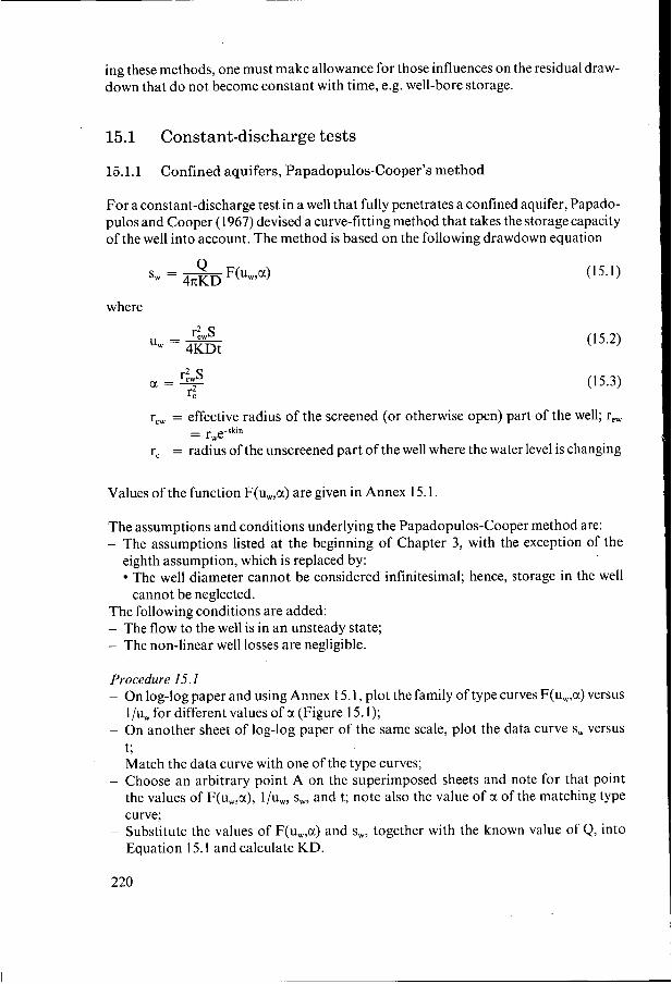
Procedure 15.1 - On log-log paper and using Annex 1 5.1, plot the family of type curves F(u,,a) versus
- On another sheet of log-log paper of the same scale, plot the data curve s, versus
- Match the data curve with one of the type curves; - Choose an arbitrary point A on the superimposed sheets and note for that point
the values of F(u,,a), l/uw, s,, and t; note also the value of a of the matching type curve;
- Substitute the values of F(u,,a) and s,, together with the known value of Q, into Equation 15.1 and calculate KD.
1 /u, for different values of a (Figure 15. I);
t;
220
Figure 15.1 Family of Papadopulos-Cooper’s type curves: F(u,,cc) versus l/u, for different values of cc
Remarks - The early-time, almost straight portion of the type curves corresponds to the period
when most of the water is derived from storage within the well. Points on the data curve that coincide with these parts of the type curves do not adequately reflect the aquifer characteristics;
- If rew is known (i.e. if the skin factor or the linear well loss coefficient B, is known), in theory a value of S can be calculated by introducing the values of Tew, l/uw, t, and KD into Equation 15.2 or by introducing the values of ro Tew, and cc into Equa- tion 15.3. The values of S calculated in these two ways should show a close agree- ment. However, since the form of the type curves differs only very slightly when c1 differs by an order of magnitude, the value of S determined by this method has questionable reliability.
15.1.2 Confined aquifers, Rushton-Singh’s ratio method
Because of the similarities of the Papadopulos-Cooper type curves (Section 15.1. l), it may be difficult to match the data curve with the appropriate type curve. To over- come this difficulty, Rushton and Singh (1983) have proposed a more sensitive curve- fitting method in which the changes in the well drawdown with time are examined. Their well-drawdown ratio is
where
s, S0.4t
22 1
s,
t
= well drawdown at time t = well drawdown at time 0.4t = time since the start of pumping
The values of this ratio are between 2.5 and 1 .O. The upper value represents the situa- tion at the beginning of the (constant discharge) test when all the pumped water is derived from well-bore storage. The lower value is approached at the end of the test when the changes in well drawdown with time have become very small.
The type curves used in the Rushton-Singh ratio method are based on values derived from a numerical model (see Annex 15.2).
Rushton-Singh’s ratio method can be used if the same assumptions as those underlying the Papadopulos-Cooper method (Section 15.1.1) are satisfied.
Procedure 15.2 - On semi-log paper and using Annex 15.2, plot the family of type curves S , / S ~ . ~ , versus
4KDt/r:, for different values of S (Figure 15.2);
s, S0.4t
gQt 2
‘ew
Figure 15.2 Family of Rushton-Singh’s type curves for a constant discharge: st/s0,4, versus 4KDt/r:, for different values of S
222
- Calculate the ratio s,/so41 from the observed drawdowns for different values of t ; - On another sheet of semi-log paper of the same scale, plot the data curve ( S , / S ~ ~ ~ )
versus t; - Superimpose the data curve on the family of type curves and, with the horizontal
coordinates s , / s O ~ , = 2.5 and 1.0 of both plots coinciding, adjust until a position is found where most of the plotted points of the data curve fall on one of the type curves;
- For 4KDt/r:, = 1.0, read the corresponding value o f t from the time axis of the data curve;
- Substitute the value o f t together with the known or estimated value of re, into 4KDt/rt, = 1 .O and calculate KD;
- Read the value of S belonging to the best-matching type curve.
15.1.3
Jacob's straight-line method (Section 3.2.2) can also be applied to single-well constant- discharge tests to estimate the aquifer transmissivity. However, not all the assumptions underlying the Jacob method are met if data from single-well tests are used. Therefore, the following additional conditions should also be satisfied: - For single-well tests in confined aquifers
Confined and leaky aquifers, Jacob's straight-line method
t 1 ~
I
I t > 25r:/KD 1
If this time condition is met, the effect of well-bore storage can be neglected; - For single-well tests in leaky aquifers
K D < t < - =- ;: ( 20";.".) 25rf
As long as t < cS/20, the influence of leakage is negligible.
Procedure 15.3 - On semi-log paper, plot the observed values of s, versus the corresponding time
- Determine the slope of the straight line, i.e. the drawdown difference As, per log
- Substitute the values of Q and As, into K D = 2.30Q/4xAsW, and calculate KD.
t (ton logarithmic scale) and draw a straight line through the plotted points;
cycle of time;
Remarks - The drawdown in the well reacts strongly to even minor variations in the discharge
rate. Therefore, a constant discharge is an essential condition for the use of the Jacob method;
- There is no need to correct the observed drawdowns for well losses before applying the Jacob method; the aquifer transmissivity is determined from drawdown differ- ences As,, which are not influenced by well losses as long as the discharge is constant;
- In theory, Jacob's method can also be applied if the well is partially penetrating, provided that late-time (t > D2S/2KD) data are used. According to Hantush (1964), the additional drawdown due to partial penetration will be constant for t > D2S/
223
2KD and hence will not influence the value of As, as used in Jacob’s method; - Instead of using the time condition t > 25rz/KD to determine when the effect of
well-bore storage can be neglected, we can use the ‘one and one-half log cycle rule of thumb’ (Ramey 1976). On a diagnostic log-log plot, the early-time data may plot as a unit-slope straight line (As,/At = l), indicating that the drawdown data are dominated by well-bore storage. According to Ramey, the end of this unit-slope straight line is about 1.5 log cycles prior to the start of the semi-log straight line as used in the Jacob method.
Example 15.1 To illustrate the Jacob method, we shall use data from a single-well constant-discharge test conducted in a leaky aquifer in Hoogezand, The Netherlands (after Mulder 1983). Mulder’s observations were made with electronic equipment that allowed very precise measurements of s, and Q to be made every five seconds. The recorded drawdown data are given in Table 15.1.
Table 15.1 Single-well constant-discharge test ‘Hoogezand’, The Netherlands (from Mulder 1983)
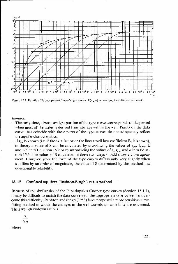
Figure 15.3 shows a semi-log plot of the drawdown s, against the corresponding time, with a straight line fitted through the plotted points. The slope of this line, As,, is 0.07 m per log cycle of time. The transmissivity is calculated from
2.’30Q - 2.30 x 28.7 x 24 = 1800m2,d 4xAs,
- 47t x 0.07 K D = -
Jacob’s straight-line method is applicable to data from single-well tests in leaky aquifers, provided that
25rf cs = < t < - 20
Substituting the value of the radius of the well (r, = 0.185 m) and the calculated transmissivity into 25rf/KD yields
Figure 15.3 Analysis of data from the single-well constant discharge test ‘Hoogezand’ with the Jacob method
According to Mulder (1 983), the values of c and S can be estimated at c = 1 O00 days and S = 4 x lo4. The drawdown in the well is not influenced by leakage as long as
c s 1000 x 4 x 104 or < 1728 20 t < - = 20
Hence, for t > 41 s, Jacob’s method can be applied to the drawdown data from the test ‘Hoogezand’.
225
15.1.4 Confined and leaky aquifers, Hurr-Worthington’s method
The unsteady-state flow to a small-diameter well pumping a confined aquifer can .be described by a modified Theis equation, provided that the non-linear well losses are negligible. The equation is written as
where r%,S u, = - 4KDt
Rearranging Equation 15.4 gives
47tKDs, Q W(U,) = ~
(15.4)
(1 5 . 5 )
(1 5.6)
Hurr (1966) demonstrated that multiplying both sides of Equation 15.6 by u, elimi- nates KD from the right-hand side of the equation
47cKDs, r:,S - 7tr%,S s, U,W(U,) = ~ x - Q 4KDt t x Q (1 5.7)
A table of corresponding values of u, and u,W(u,) is given in Annex 15.3 and a graph in Figure 15.4.
Figure 15.4 Graph of corresponding values of u, and u,W(u,)
226
Hurr (1966) outlined a procedure for estimating the transmissivity of a confined aquifer from a single drawdown observation in the pumped well. In 1981, Worthington incorporated Hurr’s procedure in a method for estimating the transmissivity of (thin) leaky aquifers from single-well drawdown data.
In leaky aquifers, the drawdown data can be affected by well losses, by well-bore storage phenomena during early pumping times, and by leakage during late pumping times.
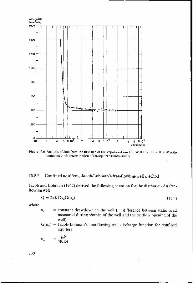
According to Worthington (1981), after the drawdown data have been corrected for non-linear well losses, one can calculate ‘pseudo-transmissivities’ by applying Hurr’s procedure to a sequence of the corrected data. Both well-bore storage effects and leakage effects reduce the drawdown in the well and will therefore lead to calcu- lated pseudo-transmissivities that are greater than the aquifer transmissivity. A semi- log plot of pseudo-transmissivities versus time shows a minimum (Figure 15.5). A flat minimum indicates the time during which the well-bore storage effects have become negligible and leakage effects have not yet manifested themselves: the minimum value of the pseudo-transmissivity gives the value of the aquifer transmissi- vity. If well-bore storage and leakage effects overlap, the lowest pseudo-transmissivity is the best estimate of a leaky aquifer’s transmissivity.
The unsteady-state drawdown data from confined aquifers can also be used to con- struct a semi-log plot of pseudo-transmissivities versus time to account for the early- time well-bore storage effects.
A well-bore
storage effects
t
B leakage well-bore leakage effects storage effects effects
t + t
Figure 15.5 Drawdown data and calculated ‘pseudo-transmissivities‘ A: Moderately affected by well storage and leakage B: Severely affected by well storage and leakage (after Worthington 1981)
227
Hurr-Worthington’s method is based on the following assumptions and conditions: - The assumptions listed at the beginning of Chapter 3, with the exception of the
first and eighth assumptions, which are replaced by: The aquifer is confined or leaky; The storage in the well cannot be neglected.
The following conditions are added: - The flow to the well is in an unsteady-state; - The non-linear well losses are negligible; - The storativity is known or can be estimated with reasonable accuracy.
Procedure 15.4 - Calculate pseudo-transmissivity values by applying the following procedure pro-
posed by Hurr to a sequence of observed drawdown data: For a single drawdown observation, calculate u,W(u,) from Equation 15.7 for known or estimated values of S and re,, and the corresponding values of t, s,, and Q; Knowing u,W(u,), determine the corresponding value of u, from Annex 15.3 or Figure 15.4; Substitute the values of u,, Tew, t, and S into Equation 15.5 and calculate the pseudo-transmissivity;
- On semi-log paper, plot the pseudo-transmissivity values versus the corresponding t (t on the logarithmic scale). Determine the minimum value of the pseudo-transmis- sivity from the plot. This is the best estimate of the aquifer’s transmissivity.
Remarks - The Hurr procedure permits the calculation of the (pseudo) transmissivity from
a single drawdown observation in the pumped well, provided that the storativity can be estimated with reasonable accuracy. The accuracy required declines with declining values of u,. For u,/S < 0.001, the influence of S on the calculated values of K D becomes negligible;
- If the non-linear well losses are not negligible, the observed unsteady-state draw- downs should be corrected before the Hurr-Worthington method is applied.
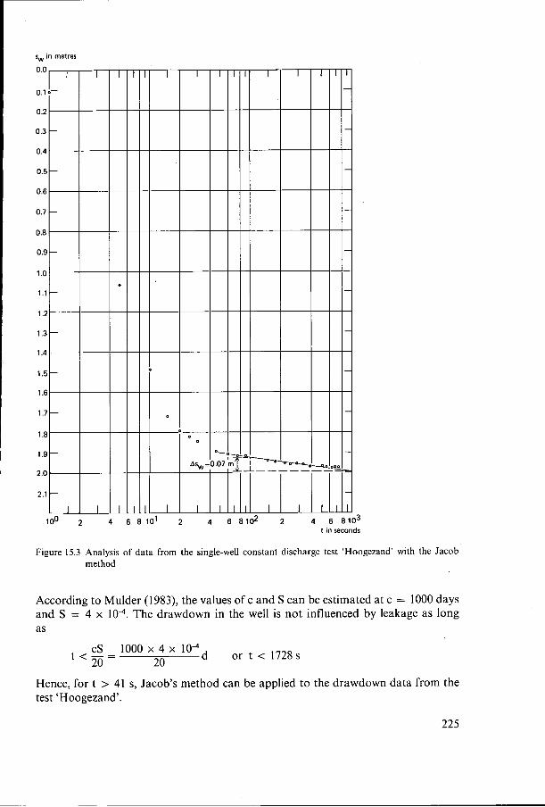
Example 15.2 To illustrate the Hurr-Worthington method, we shall use the drawdown data from the first step of the step-drawdown test ‘Well 1 ’ (see Example 14.1). During the first step, the well was pumped at a discharge rate of 1306 m3/d. Because the non-linear well losses were not negligible (CQ’ = 1.4 x I O-7 x 1 3062 = 0.239 m), the drawdown data have to be corrected according to the calculations made in Example 14.2.
To calculate (pseudo-)transmissivities, we apply Hurr’s procedure to the data from each corrected drawdown observation. First, we calculate the values of uwW(u,) from Equation 15.7 for Q = 1306 m3/d and the assumed values of S = 10“ and re, = 0.25 m. Then, using the graph of corresponding values of u, and u,W(u,) (Figure 15.4) and the table in Annex 15.3, we find the corresponding values of u,. From Equa- tion 15.5, we calculate the pseudo-transmissivities (Table 15.2).
228
Table 15.2 Pseudo-transmissivity values calculated from data obtained during the first step of step-draw- down test 'Well I '
Time s, (s,)corr*) U,W(U,) u, (pseudo) KD = s,-0.239
(min) (4 (m) (m2/d)
5 1.303 1 .O64 4.6 x IO" 3.2 x 1406 6 2.289 2.050 7.4 x 10" 5.4 IO-^ 694
8 3.345 3.106 8 . 4 ~ 6.1 x 46 1 9 3.486 3.247 7.8 x IO" 5.6 IO-^ 446
12 3.592 3.353 6 . 0 ~ IO" 4.2 x IO-' 446 14 3.627 3.388 5.2 x 10" 3.6 10-~ 446 16 3.733 3.494 4.7 x 10⁻⁶ 3.3 426 18 3.768 3.529 4.2 x 10" 2.9 10-~ 43 I 20 3.836 3.597 3.9 x IO" 2.7 IO-^ 417 25 3.873 3.634 3.1 x 10" 2.1 429 30 4.014 3.775 2.7 x 1.8 417
40 4.043 3.804 2.1 x 10" 1.4 x 402 45 4.261 4.022 I .9 x 10" 1.25 x 400 50 4.261 4.022 1 . 7 ~ IO" 1.1 409 55 4.190 3.951 1.6 x 1.05 IO-^ 390 60 4.120 3.881 1.4 x 9 x 10-8 417 70 4.120 3.88 1 1.2x 10" 7.6 x IO-' 423 80 4.226 3.987 1.1 x IO" 7.0 x IO-' 402 90 4.226 3.987 9.6 IO-^ 6.0 x IO-' 417
1 O0 4.226 3.987 8.6 x 5.4 x 10-8 417 120 4.402 4.163 7.5 4.6 x IO-' 408 I50 4.402 4.163 6.0 3.6 x IO-' 417 180 4.683 4.444 5.3 IO-^ 3.2 x IO-' 39 I
7 3.117 2.878 8 . 9 ~ 10" 6.5 x 495
I O 3.521 3.282 7.1 x 5.1 IO-^ 441
35 3.803 3.564 2.2 x 10⁻⁶ i .45 IO-^ 443
*Well loss = CQ2 = 1.4 x x (1306)' = 0.239 m
Subsequently, we plot the calculated pseudo-transmissivities versus time on semi-log paper (Figure 15.6), from which we can see that during the first eight minutes of pump- ing, the drawdown in the well was clearly affected by well-bore storage effects. Our estimate of the aquifer transmissivity is 410 m2/d.
15.2 Variable-discharge tests
15.2.1 Confined aquifers, Birsoy-Summers's method
Birsoy-Summers's method (Section 12. I . 1 ) can also be used for analyzing single-well tests with variable discharges. The parameters s and r should be replaced by s, and re, in all the equations.
229
pseudo’KD in m2/dav
t i n minutes
Figure 15.6 Analysis of data from the first step of the step-drawdown test ‘Well I ’ with the Hurr-Worth- ington method: determination of the aquifer’s transmissivity
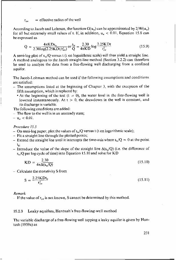
Jacob and Lohman (1952) derived the following equation for the discharge of a free- flowing well
Q = 2~cKDs,G(u,) (1 5.8)
= constant drawdown in the well (= difference between static head measured during shut-in of the well and the outflow opening of the well)
G(u,) = Jacob-Lohman’s free-flowing-well discharge function for confined aquifers
where s,
230
Tew = effective radius of the well
According to Jacob and Lohman, the function G(u,) can be approximated by 2/W(u,) for all but extremely small values of t. If, in addition, u, < 0.01, Equation 15.8 can be expressed as
A semi-log plot of s,/Q versus t (t on logarithmic scale) will thus yield a straight line. A method analogous to the Jacob straight-line method (Section 3.2.2) can therefore be used to analyze the data from a free-flowing well discharging from a confined aquifer.
The Jacob-Lohman method can be used if the following assumptions and conditions are satisfied: - The assumptions listed at the beginning of Chapter 3, with the exception of the
fifth assumption, which is replaced by: At the beginning of the test (t = O ) , the water level in the free-flowing well is lowered instantaneously. At t > O, the drawdown in the well is constant, and its discharge is variable.
The following conditions are added: - The flow to the well is in an unsteady state; - u, < 0.01.
Procedure 15.5 - On semi-log paper, plot the values of s,/Q versus t (t on logarithmic scale); - Fit a straight line through the plotted points; - Extend the straight line until it intercepts the time-axis where s,/Q = O at the point
- Introduce the value of the slope of the straight line A(s,/Q) (i.e. the difference of to;
s,/Q per log cycle of time) into Equation 15.1 O and solve for KD
2.30 47cNsw/Q)
K D =
- Calculate the storativity S from
2.25KDk S = r2,,
Remark - If the value of re, is not known, S cannot be determined by this method.
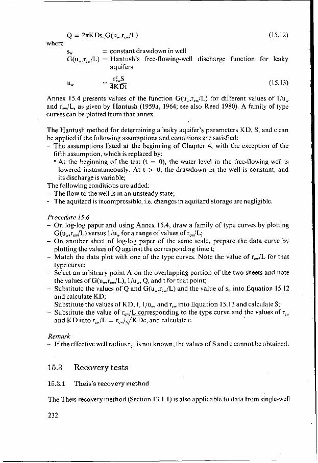
The variable discharge of a free-flowing well tapping a leaky aquifer is given by Han- tush (1959a) as
23 1
Q = ~KKDs,G(~,,~,,/L)
S W
G(uw,rew/L) = Hantush’s free-flowing-well discharge function for leaky
( 1 5.12) where
= constant drawdown in well
aquifers
(1 5.1 3)
Annex 15.4 presents values of the function G(uw,rew/L) for different values of l/uw and rew/L, as given by Hantush (1959a, 1964; see also Reed 1980). A family of type curves can be plotted from that annex.
The Hantush method for determining a leaky aquifer’s parameters KD, S, and c can be applied if the following assumptions and conditions are satisfied: - The assumptions listed at the beginning of Chapter 4, with the exception of the
fifth assumption, which is replaced by: At the beginning of the test (t = O), the water level in the free-flowing well is lowered instantaneously. At t > O , the drawdown in the well is constant, and its discharge is variable;
The following conditions are added: - The flow to the well is in an unsteady state; - The aquitard is incompressible, i.e. changes in aquitard storage are negligible.
Procedure 15.6 - On log-log paper and using Annex 15.4, draw a family of type curves by plotting
- On another sheet of log-log paper of the same scale, prepare the data curve by
- Match the data plot with one of the type curves. Note the value of rew/L for that
- Select an arbitrary point A on the overlapping portion of the two sheets and note
- Substitute the values of Q and G(uw,rew/L) and the value of s, into Equation 15.12
- Substitute the values of KD, t, l/uw, and rew into Equation 15.13 and calculate S; - Substitute the value of rew/L corresponding to the type curve and the values of rew
G(uw,rew/L) versus l /uw for a range of values of rew/L;
plotting the values of Q against the corresponding time t;
type curve;
the values of G(uw,rew/L), l/uw, Q, and t for that point;
and calculate KD;
and K D into rew/L = rew/.\/I(Dc, and calculate c.
Remark - If the effective well radius rew is not known, the values of S and c cannot be obtained.
15.3 Recovery tests
15.3.1 Theis’s recovery method
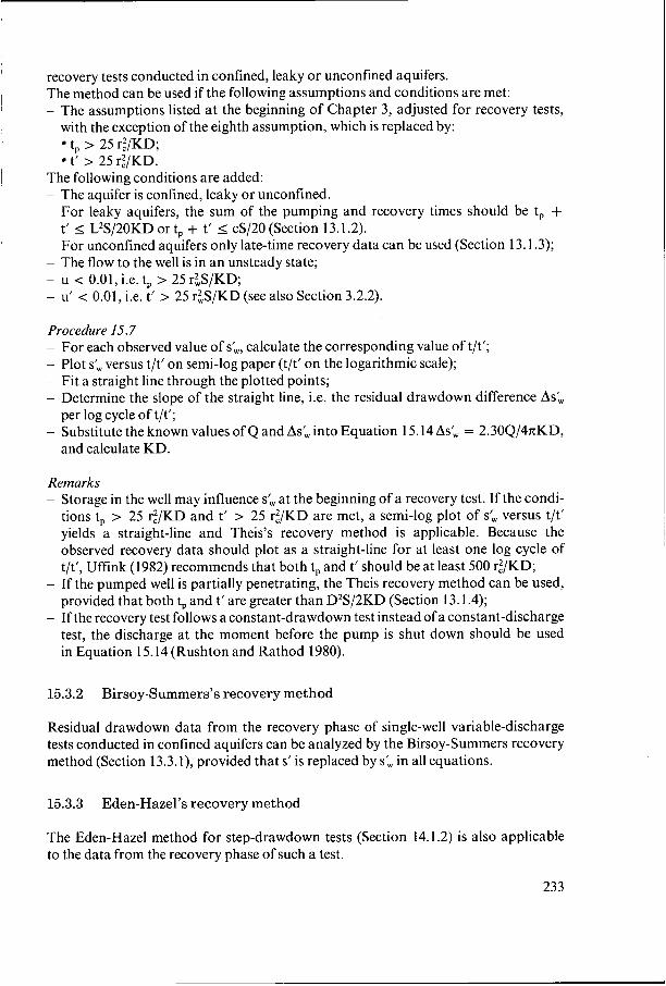
The Theis recovery method (Section 13.1.1) is also applicable to data from single-well
232
recovery tests conducted in confined, leaky or unconfined aquifers. The method can be used if the following assumptions and conditions are met: - The assumptions listed at the beginning of Chapter 3, adjusted for recovery tests,
with the exception of the eighth assumption, which is replaced by: t, > 25 r:/KD; t’ > 25 rf/KD.
The following conditions are added: - The aquifer is confined, leaky or unconfined.
For leaky aquifers, the sum of the pumping and recovery times should be t, + t’ < L2S/20KD or t, + t’ < cS/20 (Section 13.1.2). For unconfined aquifers only late-time recovery data can be used (Section 13.1.3);
- The flow to the well is in an unsteady state; - u < 0.01, i.e. t, > 25 riS/KD; - u’ < 0.01, i.e. t’ > 25 r$S/KD (see also Section 3.2.2).
Procedure 15.7 - For each observed value of sk, calculate the corresponding value of t/t’; - Plot sk versus t/t’ on semi-log paper (t/t’ on the logarithmic scale); - Fit a straight line through the plotted points; - Determine the slope of the straight line, i.e. the residual drawdown difference Ask
- Substitute the known values of Q and Ask into Equation 15.14 Ask = 2.30Q/4nKD, per log cycle of t/t’;
and calculate KD.
Remarks - Storage in the well may influence s i at the beginning of a recovery test. If the condi-
tions t, > 25 r:/KD and t’ > 25 rf/KD are met, a semi-log plot of s; versus t/t’ yields a straight-line and Theis’s recovery method is applicable. Because the observed recovery data should plot as a straight-line for at least one log cycle of t/t’, Uffink (1 982) recommends that both t, and t’ should be at least 500 rf/KD;
- If the pumped well is partially penetrating, the Theis recovery method can be used, provided that both t, and t’ are greater than D2S/2KD (Section 13.1.4);
- If the recovery test follows a constant-drawdown test instead of a constant-discharge test, the discharge at the moment before the pump is shut down should be used in Equation 15.14 (Rushton and Rathod 1980).
15.3.2 Birsoy-Summers’s recovery method
Residual drawdown data from the recovery phase of single-well variable-discharge tests conducted in confined aquifers can be analyzed by the Birsoy-Summers recovery method (Section 13.3.l), provided that s’ is replaced by s; in all equations.
15.3.3 Eden-Hazel’s recovery method
The Eden-Hazel method for step-drawdown tests (Section 14.1.2) is also applicable to the data from the recovery phase of such a test.
233
The Eden-Hazel recovery method can be used if the following assumptions and condi- tions are met: - The assumptions listed at the beginning of Chapter 3, as adjusted for recovery tests,
with the exception of the fifth assumption, which is replaced by: Prior to the recovery test, the aquifer is pumped step-wise.
The following conditions are added: - The flow to the well is in unsteady state; - u < 0.01 (see Section 3.2.2); - u’ < 0.01.
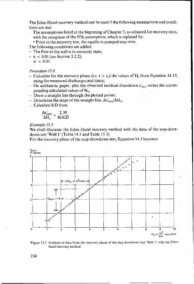
Procedure 15.8 - Calculate for the recovery phase (i.e. t > t,) the values of H, from Equation 14.15,
- On arithmetic paper, plot the observed residual drawdown s&(,) versus the corres-
- Draw a straight line through the plotted points; - Determine the slope of the straight line, As&(,)/AH,; - Calculate K D from
using the measured discharges and times;
ponding calculated values of H,;
Example 15.3 We shall illustrate the Eden-Hazel recovery method with the data of the step-draw- down test ‘Well I ’ (Table 14.1 and Table 15.3). For the recovery phase of the step-drawdown test, Equation 14.5 becomes
%In) in metres
H, in-$ min Log (min)
Figure 15.7 Analysis of data from the recovery phase of the step-drawdown test ‘Well I’ with the Eden- Hazel recovery method
Table 15.3 shows the result of the calculations for t > t,. Figure 15.7 gives the arithmetic plot of the s&(., versus H,. The slope of the straight line is
AH, 2 1440 - 5.2 x 10⁴d/m2 1
2’30 - 352m2/d 4x x 5.2 x lo4 - The transmissivity KD =
Table 15.3 Values of H, calculated for the recovery phase of step-drawdown test ‘Well I’