17 :-15612 MICTFOWAUE LANDINC Y'T[M MU) MATHEMATICAL MODEL 1INSTALLATION MANUAL(U) MSI EICSIC WASHINCTON DC

PODJ'NE' MAY 87 DOTIFAA/CT- 1N7/17 DTFA@3-86-,'-655N,:LA::IFIED T 12/5 M

51F M

II 11111 1 0 L~ 28111Q. JL2

- .

MICROCOPY RESOLUTrION TEST CHARTNATIONAL BUJREAU OF STANDARDO$163 -A

~ i0n FILE WuPY

N

Microwave Landing System00 (MLS) Mathematical ModelInstallation Manual

DD

May 1987

DOT/FAAICT-TN87/17

This document is available to the U.S. publicthrough the National Technical Information

Srice, Springfield, Virginia 22161.

JYWIEU NcrT EM-N.'.-T AApproved for public relecael

Dibtribution Unlimited

Technical CenterAtlantic City Airport, N.J. 08405

___ 87 10 20 085

NOTICE

This document is disseminated under the sponsorship ofthe Department of Transportation in the interest ofinformation exchange. The United States Governmentassumes no liability for the contents or use thereof.

The United States Government does not endorse productsor manufacturers. Trade or manufacturer's names appearherein solely because they are considered essential tothe object of this report.

Tgechical. Nowe Deoma91. PIIg.1. Repett C..oiGeo eee Aesoosion Me. 3. ircipients Carol"g Ne.

DOT/FAA/CT-TN87/174. Title end Siplbile eetOMICROWAVE LANDING SYSTEM (MLS) MATHEMATICAL Mayt 1987

MODEL INSTALLATION MANUAL Ma 1987coj

ACT- 14 07. Aimes) . Pehegfnil ro tegeaeien Newte N.

Jesse D. Jones DOT/FAA/CT-TN/S 7/179. Performing Orgui aehle MsondAd.. I*. We&~ Unit Me. (TRAS)Department ofelTransporationFederal Aviation Administration . ofr"fGeaN.Technical Center T0603Nt ee. eAtlantic City International Airport, N.J. 08405 1-T6o0Rpr3N ~ o~ ovri

12. heneecwing Age.., MK~ end Addeoee Technical NoteDepartment of TransportationJue18-Fbray97Federal Aviation AdministrationJue18-Fbray97Program Engineering and Maintenance Service Id. Seeei.g Ageriew CedeWashington,_D.C.__20590 _______

15. supplen"Aee Noes

6.Abstrest

This Technical Note provides requirements and guidance for the installation ofthe baselined microwave landing system (MLS) mathematical model. This modeloriginated at the Massachusetts Institute of Technology, Lincoln Laboratory,during the late 1970's, and has been revised and baselined to facilitate futuresoftware support and improvements A majority of the work in developing thisTechnical Note was performed under contract DTFAO3-86-C-00055, Task B-2 by:

MSl Services Incorporated600 Maryland Avenue, S.W.Suite 695Washington, D.C. 20024

Q~7. Key words 0iOs.'eboti.. Stete~enetmicrowave Ladn System) This document is available to the U.S.

Matemtia Mo/l 'C -0 public through the National TechnicalIsaatoMau/LSMathematical Mdl Information Service, Springfield, Va.

model~ 22161

I9. Se....,ey Cloede. thi owel$ X. see~ Clotted. (of * Ibs pe) 21. Me. of Peges 22. Pie

P.Uncasfe Unclassified 25

FomDOT F 1MO.7 (S1-72)*eedn... eltepg.,esd

TABLE OF CONTENTS

Page

EXECUTIVE SUMMARY v

INTRODUCTION 1

Purpose 1

Intended Audience 1

REQUIREMENTS I

Hardware Requirements 1Software Requirements 2Storage Requirements 2

DISTRIBUTION MEDIA AIlD LAYOUT 3

GENERAL PROCEDURES 3

ABOUT THE APPENDIXES 4

APPENDIXES

A - Graphics Interface Software Specifications

B - IBM/MVS/TSO InstallationsC - DEC/VAX 11/750/780 InstallationsD - UNIX System V Systems Installations

z,7

-Ll

-iti

EXECUTIVE SUMMARY

This Technical Note provides an estimate of system requirements and installationguidance for the baselined microwave landing system (MILS) mathematical model. Thismodel was originally developed by the Massachusetts Institute of Technology, LincolnLaboratory, during the late 1970's. Different users of the model subsequentlyobtained copies of the model with various levels of improvements. Therefore, tofacilitate future software support and improvements, the Federal AviationAdministration (FAA) contracted to have the model baselined with all knownimprovements and to make the data input user friendly.

v

INTRODUCTION

PURPOSE.

The purpose of this manual is to provide the user with instructions that will permitthe installation of the microwave landing system (MLS) Lincoln Laboratory simulationsoftware at the user's computer facility. It is intended that the procedure formaking revisions to the model will be accomplished by a reinstallation and,therefore, "installation" and "system update" will use the same procedure asdescribed in this manual.

A general procedures section is included to give the user or the person installingthe simulation a basic idea of the steps that are required in the installationprocess. This section will NOT provide system specific procedures because these willbe different for each installation, i.e., the installation of the software on an IBM3033 mainframe will require different commands and utilities than installation on a

* DEC VA~k 11/780.

Appendixes have been furnished to provide some system specific examples of computerutilities and setups that could be employed to actually accomplish the installationat a given computer facility.

A specification for user supplied graphics software is included in appendix A.

IlrT- DED AUDIENCE.

The manual is written for someone with computer background. In order to implementthe procedures described in this manual, the user will have to have access to thetarget computer system and be familiar vith some of the system utilities (e.g.,editors and compilers) that reside In the system. Some of the necessary informationcan probably be obtained from the system administrator, or technical staff if thefacility happens to be a large one.

REQUIREMENTS

HARDWARE REQUIREMENTS .

* The computer that is to serve as the target system must have the following hardwareelements:

1. 1/2 inch 9-track 1600 bits per inch (bpi) tape drive

2. 1 megabyte applications program memory

3. Floating point processor (not required but recommended)

4. Graphical output device.

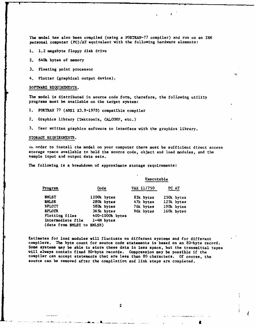
The model has also been compiled (using a FORTRAN-77 compiler) and run on an IBMpersonal computer (PC)/AT equivalent with the following hardware elements:

1. 1.2 megabyte floppy disk drive

2. 640k bytes of memory

3. Floating point processor

4. Plotter (graphical output device).

SOFTWARE REQUI2EME11TS.

The model is distributed in source code form, therefore, the following utilityprograms must be available on the target system:

1. FORTRAN4 77 (ANSI X3.9-1978) compatible compiler

2. Graphics library (Tektronix, CALCOMP, etc.)

3. User written graphics software to interface with the graphics library.

STORAGE REQUIREMENTS.

ii, order to install the model on your computer there must be sufficient direct accessstorage space available to hold the source code, object and load modules, and thesample input and output data sets.

The following is a breakdown of approximate storage requirements:

Executable

Program Code VAX 11/750 PC AT

BMLST 1200k bytes 83k bytes 250k bytesBMLSR 280k bytes 47k bytes 125k bytesBPLOTT 580k bytes 76k bytes 190k bytesBPLOTR 365k bytes 96k bytes 160k bytesPlotting files 400-1000k bytesIntermediate file 1-4M bytes(data from BMLST to BMLSR)

Estimates for load modules will fluctuate on different systems and for differentcompilers. The byte count for source code statements is based on an 80-byte record.Some systems may be able to store these data in less space, but the transmittal tapeswill always contain fixed 80-byte records. Compression may be possible if thecompiler can accept statements that are less than 80 characters. Of course, thesource can be removed after the compilation and link steps are completed.

2

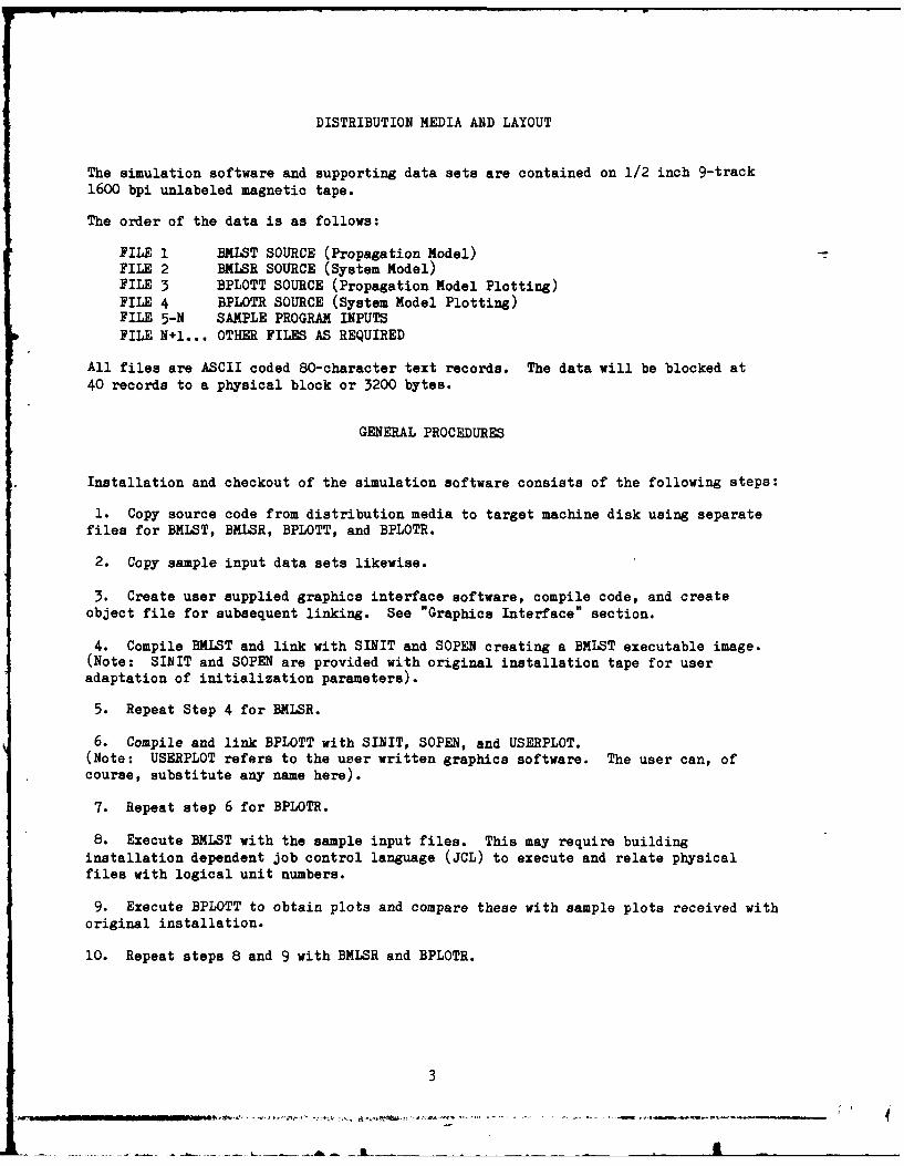
DISTRIBUTION MEDIA AND LAYOUT

The simulation software and supporting data sets are contained on 1/2 inch 9-track1600 bpi unlabeled magnetic tape.

The order of the data is as follows:

FILE 1 BMLST SOURCE (Propagation Model)FILE 2 BMLSR SOURCE (System Model)FILE 3 BPLOTT SOURCE (Propagation Model Plotting)FILE 4 BPLOTR SOURCE (System Model Plotting)FILE 5-N SAMPLE PROGRAM INPUTS

FILE N+l... OTHER FILES AS REQUIRED

All files are ASCII coded 80-character text records. The data will be blocked at40 records to a physical block or 3200 bytes.

GENERAL PROCEDURES

Installation and checkout of the simulation software consists of the following steps:

1. Copy source code from distribution media to target machine disk using separatefiles for BMLST, BMLSR, BPLOTT, and BPLOTR.

2. Copy sample input data sets likewise.

3. Create user supplied graphics interface software, compile code, and createobject file for subsequent linking. See "Graphics Interface" section.

4. Compile BMLST and link with SINIT and SOPEN creating a BMLST executable image.(Note: SINIT and SOPEN are provided with original installation tape for useradaptation of initialization parameters).

5. Repeat Step 4 for BMLSR.

6. Compile and link BPLOTT with SINIT, SOPEN, and USERPLOT.(Note: USERPLOT refers to the user written graphics software. The user can, ofcourse, substitute any name here).

7. Repeat step 6 for BPLOTR.

8. Execute BMLST with the sample input files. This may require buildinginstallation dependent job control language (JCL) to execute and relate physicalfiles with logical unit numbers.

9. Execute BPLOTT to obtain plots and compare these with sample plots received withoriginal installation.

10. Repeat steps 8 and 9 with BMLSR and BPLOTR.

3

11. If the model fails to complete execution or produces strange results notmatching the sample outputs, save the output and consult with your installationtechnical staff for probable cause of the error. Report the failure and any knowncauses to the Guidance and Airborne Systems Branch, ACT-140, FAA Technical Center,Atlantic City International Airport, N.J. 08405.

12. Create a "secure" backup copy of all installed software.

ABOUT THE APPENDIXES

The following appendixes describe in some detail the required graphics interfacesoftware and the necessary computer setups for installing the simulation software andsample input/output data sets.

The sample installation procedures have been written in as "generic" a form as ispossible. All computer installations tend to tailor their job control language fortheir installation. This means that the setups that are shown here as samples willrequire slight modification at any given site.

4

APPENDIX A

GRAPHICS INTERFACE SOFTWARE SPECIFICATIONS

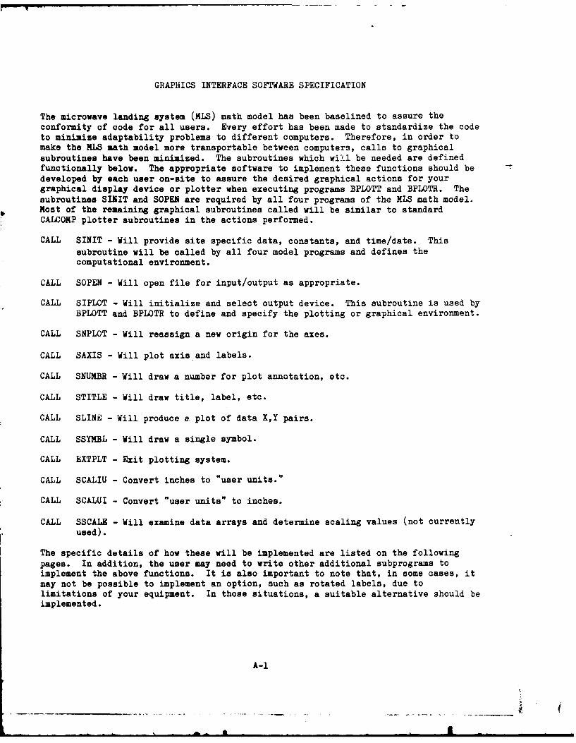
GRAPHICS INTERFACE SOFTWARE SPECIFICATION

The microwave landing system (MLS) math model has been baselined to assure theconformity of code for all users. Every effort has been made to standardize the codeto minimize adaptability problems to different computers. Therefore, in order tomake the MLS math model more transportable between computers, calls to graphicalsubroutines have been minimized. The subroutines which will be needed are definedfunctionally below. The appropriate software to implement these functions should bedeveloped by each user on-site to assure the desired graphical actions for yourgraphical display device or plotter when executing programs BPLOTT and BPLOTR. Thesubroutines SINIT and SOPEN are required by all four programs of the MLS math model.Most of the remaining graphical subroutines called will be similar to standardCALCOMP plotter subroutines in the actions performed.

CALL SINIT - Will provide site specific data, constants, and time/date. This

subroutine will be called by all four model programs and defines thecomputational environment.

CALL SOPEN - Will open file for input/output as appropriate.

CALL SIPLOT - Will initialize and select output device. This subroutine is used by

BPLOTT and BPLOTR to define and specify the plotting or graphical environment.

CALL SNPLOT - Will reassign a new origin for the axes.

CALL SAXIS - Will plot axis and labels.

CALL SNUMBR - Will draw a number for plot annotation, etc.

CALL STITLE - Will draw title, label, etc.

CALL SLINE - Will produce a plot of data X,Y pairs.

CALL SSYMBL - Will draw a single symbol.

CALL EXTPLT - Exit plotting system.

CALL SCALIU - Convert inches to "user units."

CALL SCALUI - Convert "user units" to inches.

CALL SSCALE - Will examine data arrays and determine scaling values (not currentlyused).

The specific details of how these will be implemented are listed on the followingpages. In addition, the user may need to write other additional subprograms toimplement the above functions. It is also important to note that, in some cases, itmay not be possible to implement an option, such as rotated labels, due tolimitations of your equipment. In those situations, a suitable alternative should beimplemented.

A-1

_ _ _ _ _ 4

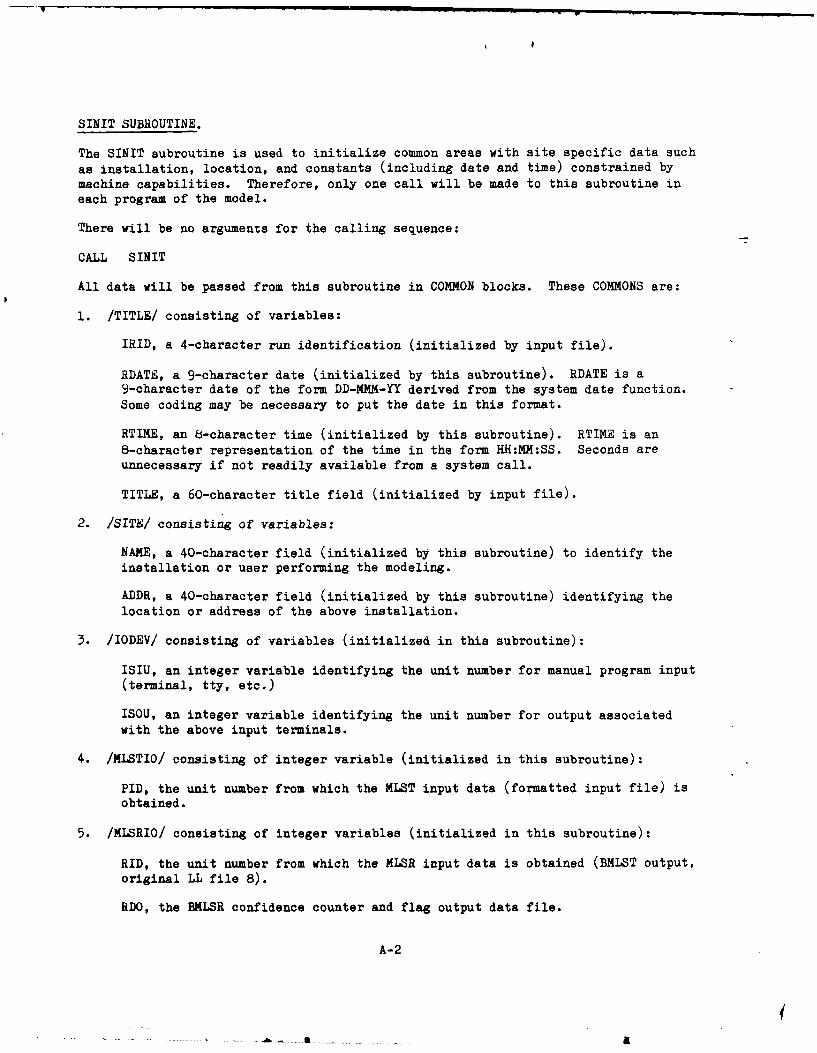
SINIT SUBROUTINE.

The SINIT subroutine is used to initialize common areas with site specific data such

as installation, location, and constants (including date and time) constrained by

machine capabilities. Therefore, only one call will be made to this subroutine ineach program of the model.

There will be no arguments for the calling sequence:

CALL SINIT

All data will be passed from this subroutine in COMMON blocks. These COMMONS are:

1. /TITLE/ consisting of variables:

IRID, a 4-character run identification (initialized by input file).

RDATE, a 9-character date (initialized by this subroutine). RDATE is a9-character date of the form DD-MMM-YY derived from the system date function.

Some coding may be necessary to put the date in this format.

RTIME, an 8-character time (initialized by this subroutine). RTIME is an

8-character representation of the time in the form HH:MM:SS. Seconds areunnecessary if not readily available from a system call.

TITLE, a 60-character title field (initialized by input file).

2. /SITE/ consisting of variables:

NAME, a 40-character field (initialized by this subroutine) to identify theinstallation or user performing the modeling.

ADDR, a 40-character field (initialized by this subroutine) identifying thelocation or address of the above installation.

3. /IODEV/ consisting of variables (initialized in this subroutine):

ISIU, an integer variable identifying the unit number for manual program input(terminal, tty, etc.)

ISOU, an integer variable identifying the unit number for output associatedwith the above input terminals.

4. /MLSTIO/ consisting of integer variable (initialized in this subroutine):

PID, the unit number from which the MLST input data (formatted input file) isobtained.

5. /MLSRIO/ consisting of integer variables (initialized in this subroutine):

RID, the unit number from which the MLSR input data is obtained (BMLST output,original LL file 8).

RDO, the BMLSR confidence counter and flag output data file.

A-2

.. .. . . .... . . .. ...... . . .. .. .. .. .44

6. /PMLSTD/ consisting of integer variables (initialized in this subroutine):

PPID, the unit number for the input data to be plotted as MLST diagnosticplots (BMLST graphical output data).

PPOD, the unit number used for the plotter or other display device.

7. /PMLSRD/ consisting of integer variables (initialized in this subroutine):

PRID, the unit number for the input data (original LL file 12) to be plotted aserror data.

PROD, the unit number used for the plotter or other display device.

8. /MFPIO/ consisting of integer variables (initialized in this subroutine):

MFID, the unit number for measured flight path input data.

SUBROUTINE SOPEN.

The SOPEN subroutine is used to open files for input/output. This subroutine iscalled once for each file to be opened.

The calling sequence

CALL SOPEN (LDEV, NAME, STAT, RLEN)

has four argument3 as follows:

LDEV: an integer variable, is the logical device number to be associated withthe input/output file. This number will be one of the variables assigneda value by SINIT and will be supplied to SOPEN by the subroutine call.

NAME: a character variable of length 40 bytes specifying the file name to beassociated with LDEV. This file name is specified by the user during thequestion and answer sequence when the program is run.

STAT: a character variable of length 3 bytes specifying the status of the filebeing opened. STAT will be given a value of either 'NEW' or 'OLD' by the callto SOPEN. The user can change the value of STAT within SOPEN, if necessary.

RLEN: an integer variable indicating the record length of the file beingopened. RLEN will be given a value in the call to SOPEN. The user can changethe value of RLEN in SOPEN, if necessary.

This subroutine should include the labeled common blocks MLSTIO, MLSRIO, PMLST,PMLSRD, and MFPIO which contain the variables initialized by SINIT to the appropriatelogical device numbers. These will be passed to SOPEN along with an appropriatestatus and record length and the file name supplied by the user interactively. It issuggested that SOPEN contain error traps to allow the user to change the file nameand/or the status without terminating the program.

A-3

Ia

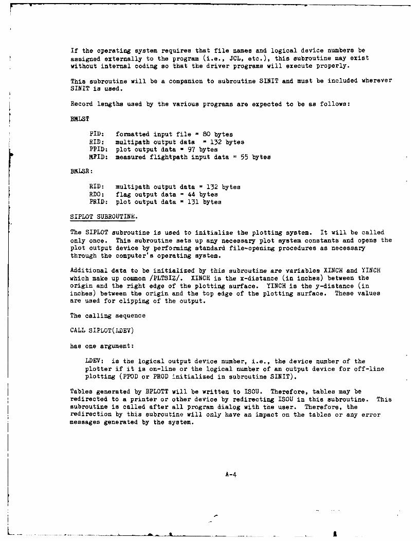
If the operating system requires that file names and logical device numbers be

assigned externally to the program (i.e., JCL, etc.), this subroutine may existwithout internal coding so that the driver programs will execute properly.

This subroutine will be a companion to subroutine SINIT and must be included whereverSINIT is used.

Record lengths used by the various programs are expected to be as follows:

BMLST

PID: formatted input file = 80 bytesRID: multipath output data = 132 bytesPPID: plot output data = 97 bytesKFID: measured flightpath input data = 55 bytes

BMLSR:

RID: multipath output data = 132 bytesRDO: flag output data = 44 bytesPRID: plot output data = 131 bytes

SIPLOT SUBROUTINE.

The SIPLOT subroutine is used to initialize the plotting system. It will be called

only once. This subroutine sets up any necessary plot system constants and opens theplot output device by performing standard file-opening procedures as necessarythrough the computer's operating system.

Additional data to be initialized by this subroutine are variables XINCH and YINCHwhich make up common /PLTSIZ/. XINCH is the x-distance (in inches) between theorigin and the right edge of the plotting surface. YINCH is the y-distance (ininches) between the origin and the top edge of the plotting surface. These valuesare used for clipping of the output.

The calling sequence

CALL SIPLOT(LDEV)

has one argument:

LDEV: is the logical output device number, i.e., the device number of theplotter if it is on-line or the logical number of an output device for off-lineplotting (PPOD or PROD initialized in subroutine SINIT).

Tables generated by BPLOTT will be written to ISOU. Therefore, tables may beredirected to a printer or other device by redirecting ISOU in this subroutine. Thissubroutine is called after all program dialog with tne user. Therefore, theredirection by this subroutine will only have an impact on the tables or any error

messages generated by the system.

A-4

SNPLOT SUBROUTINE.

The SNPLOT subroutine is used to reassign the origin for the X and Y axes and/or toperform a page advance (clear screen) or whatever command is needed to provide aclean surface for the preparation of a new plot. The calling sequence

CALL SNPLOT (IDEV)

has one argument:

IDEY: is the logical output device number to which the current output is beingdirected, i.e., tables will be directed to ISOU, whereas plots will be directedto PPOD or PROD.

This subroutine is called with IDEV=ISOU for outputting of tables, and IDEV=PPODor PROD when displaying plots. Thus, the user may develop the software for thissubroutine to advance the printer or plotter as required.

SAXIS SUBROUTINE.

Most graphs require axis lines and scales to indicate the orientation and values ofthe plotted data points. The type of scaled axis produced by the SAXIS subroutine isa line at 00 or 900 angle, (X or Y) divided into one-inch segments. This callalso annotates the divisions with appropriate scale values and labels the axis with acentered title. SAXIS is called separately for each X and Y axis.

The five arguments in the calling sequence are as follows:

CALL SAXIS (AXIS, LABL, NCIAR, FIRSTV, DELTAV)

AXIS: is a character variable (X or Y) specifying which axis is to be drawn. Theaxis length will be 9 inches for X and 6 inches for Y assuming an 8 1/2 x 11 inchplotting surface. Otherwise, the X-axis should be centered and occupy 9/llths ofthe plot X-dimension. The Y-axis would then span a ratio 6/8.5 of theY-dimension beginning 1/8.5 from the bottom of the plot.

LABL: is the axis label, which is centered and placed parallel to the axis line.This parameter is a character variable of not more than 40 characters. Allannotation appears on the negative (clockwise) side of the X-axis. Allannotation appears on the positive (counterclockwise) side of the Y-axis.

NCHAR: is the number of characters in the label.

FIRSTV: is the starting value which will appear at the first tick mark (origin)on the axis. This value will be specified by the model input data file in orderto standardize plotting scales.

DELTAV: represents the number of data units per inch of axis. This value(increment or decrement), which is added to FIRSTV for each succeeding 1-inchdivision along the axis, will also be specified in the model input data file.

A-5

SNUMBR SUBROUTINE.

SNUMBR converts a floating-point number to the appropriate decimal equivalent so thatthe number may be plotted in the FORTRAN F-type format.

The SNUMBR calling sequence has six arguments:

CALL SNUKBR (XPAGE, YPAGE, HEIGHT, FPN, ANGLE, +.NDEC)

XPAGE, YPAGE: are the coordinates of the number in user data units.

HEIGHT: is the height (and width), in inches,of the symbol to be drawn.

FPN: is the floating-point number that is to be converted and plotted.

ANGLE: is the angle in degrees from the X-axis, at which the annotation is tobe plotted. If ANGLE-O.O, the number will be plotted right side up andparallel to the X-axis. Note: Implementation of rotated numbers at any anglemay not be feasible with all graphics packages.

+NDEC: controls the precision of the conversion of the number FPN. If thevalue of NDEC greater than 0, it specifies the number of digits to the rightof the decimal point that are to be converted and plotted, after properrounding. For example, assume an internal value (perhaps in binary form) of-0.12345678 x 103. If NDEC were 2, the plotted number would be -123.46.

STITLE SUBROUTINE.

The STITLE subroutine produces plot annotation at any angle and in practically anysize. This call can be used to draw text such titles, captions, and legends.

The STITLE calling sequence has six arguments:

CALL STITLE (XPAGE, YPAGE, HEIGHT, CHAR, L, ANGLE)

XPAGE, YPAGE: are the coordinates, in inches, of the lower left-hand corner(before character rotation) of the first character to be produced. The pen isup while moving to this point.

HEIGHT: is the height, in inches, of the character to be plotted. Theplotting routines assume the width of a character, including spacing, isnormally the same as the height (e.g., a string of 10 characters, 0.14 inchhigh is 1.4 inches wide).

CHAR: is the text, in character representation to be used for annotation. Thecharacter(s) must be contiguous in a single variable. This variable is to bedimensioned for 60 characters.

L: the number of characters in the title.

A-6

!I

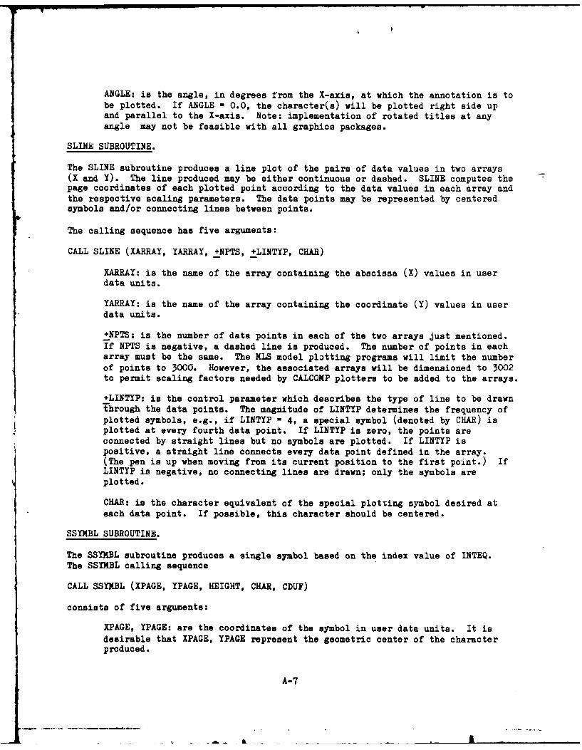
ANGLE: is the angle, in degrees from the X-axis, at which the annotation is tobe plotted. If ANGLE = 0.0, the character(s) will be plotted right side upand parallel to the X-axis. Note: implementation of rotated titles at anyangle may not be feasible with all graphics packages.

SLINE SUBROUTINE.

The SLINE subroutine produces a line plot of the pairs of data values in two arrays(X and Y). The line produced may be either continuous or dashed. SLINE computes thepage coordinates of each plotted point according to the data values in each array andthe respective scaling parameters. The data points may be represented by centeredsymbols and/or connecting lines between points.

The calling sequence has five arguments:

CALL SLINE (XARRAY, YARRAY, +NPTS, +LINTYP, CHAR)

XARRAY: is the name of the array containing the abscissa (X) values in userdata units.

YARRAY: is the name of the array containing the coordinate (Y) values in userdata units.

+NPTS: is the number of data points in each of the two arrays just mentioned.If NPTS is negative, a dashed line is produced. The number of points in eacharray must be the same. The MLS model platting programs will limit the numberof points to 3000. However, the associated arrays will be dimensioned to 3002to permit scaling factors needed by CALCOMP plotters to be added to the arrays.

+LINTYP: is the control parameter which describes the type of line to be drawnthrough the data points. The magnitude of LINTYP determines the frequency ofplotted symbols, e.g., if LINTYP - 4, a special symbol (denoted by CHAR) isplotted at every fourth data point. If LINTYP is zero, the points areconnected by straight lines but no symbols are plotted. If LINTYP ispositive, a straight line connects every data point defined in the array.(The pen is up when moving from its current position to the first point.) IfLINTYP is negative, no connecting lines are drawn; only the symbols areplotted.

CHAR: is the character equivalent of the special plotting symbol desired ateach data point. If possible, this character should be centered.

SSYMBL SUBROUTINE.

The SSYMBL subroutine produces a single symbol based on the index value of INTEQ.The SSYMBL calling sequence

CALL SSYMBL (XPAGE, YPAGE, HEIGHT, CHAR, CDUF)

consists of five arguments:

XPAGE, YPAGE: are the coordinates of the symbol in user data units. It isdesirable that XPAGE, YPAGE represent the geometric center of the characterproduced.

A-7

HEIGHT: is the height (and width), in inches, of the symbol to be drawn.CHAR: is the character equivalent of the desired symbol.

CDUF: is a character argument which determines whether the pen is up or down

during the move to XPAGE, YPAGE.

Where:

U - the pen is up during the move, after which a single symbol is produced.

D - the pen is down during the move, after which a single symbol is produced.

EXTPLT SUBROUTINE.

The EXTPLT subroutine is executed to exit the plotting programs. The calling

sequence:

CALL EXTPLT

has no arguments, and will be the last call in the plotting driver program. This

subroutine will be used to close files and plotting devices. Any device numbersnecessary to close the users plotting system should be passed into this subroutine bythe use of labeled common areas initialized and/or defined by SIPLOT.

SCALIU SUBROUTINE.

The SCALIU subroutine inputs an X, Y coordinate pair in inches and provides anequivalent X, Y coordinate pair in "user data units." The calling sequence:

CALL SCALIU (XI, YI, X, Y)

consists of the arguments:

XI, YI: X and Y coordinate pair in inches referenced to the plot origin.

X, Y: equivalent X-Y location in "user data units."

SCALUI SUBROUTINE.

The SCALUI subroutine takes an X, Y coordinate pair in "user data units" and provides

the equivalent coordinates in inches. The calling sequence:

CALL SCALUI (X, Y, XI, YI)

consists of the arguments:

X, Y: X and Y coordinate pair in "user data units"

XI, YI: equivalent location in inches referenced to plot origin.

A-8

SSCALE SUBROUTINE. (Not currently used)

Typically, the user's program will accumulate plotting data in two arrays:

An array of independent variables, Xi

An array of dependent variables, Xi = f(Xi )

It would be unusual if the range of values in each array corresponded exactly withthe number of inches available in the actual plotting area. For some problems the

range of data is predictable. The MLS math model has predetermined standard scalefactors for use in drawing the axes and plotting the data points on the graph. Forspecial applications, however, these factors may not be known in advance.

Therefore, the SSCALE subroutine is used to examine the data valueb in any array and

to determine a starting value (FIRSTV, minimum or maximum) and a scaliug factor(DELTAV, positive or negative) such that:

1. The scale annotation drawn by the SAXIS subroutine at each division will properly

represent the range of real data values in the array.

2. The data points, when plotted by the SLINE subroutine, will fit in a givenplotting area. These two values are computed and returned by the call to SSCALE.

The scaling factor (DELTAV) that is computed represents the number of data units per

inch of axis, but is adjusted so that there is always an interval of 1, 2, 4, 5, or8 x 10 (where n is an exponent consistent with the original unadjusted scalingfactor). Thus, an array may have a range of values from 301 to 912, to be plottedover an axis of 10 inches. The unadjusted scaling factor is (912-301)/10 = 61.1units/inch. The adjusted DELTAV would be 8 x 101 = 80.

The starting value (FIRSTV), which will appear as the first annotation on the axis,is computed as some multiple of DELTAV that is equal to or outside the limits of thedata in the array. For the example given above, if a minimum is wanted for FIRSTV,240 would be chosen as the best value. If a maximum is desired instead, 960 would beselected. In some instances, FIRSTV is selected as a downward-rounded value of thelowest actual data, and in other instances, the DELTAV ia adjusted upwards. Anattempt is then made to center the data.

There are six arguments in the calling sequence:

CALL SSCALE (ARRAY, AXLEN, NPTS, +INC, FIRSTV, DELTAV)

ARRAY: is the first element of the array of data points to be examined.

AXLEN: is the length of the axis (in inches) to which the data is to bescaled. Its value must be greater than 1.0 inch.

NPTS: is the number of data values to be scanned in the array.

+INC: is an integer whose magnitude is used by SSCALE as the increment withWhich to select the data values to be scanned in the array.

Normally INC - 1; if it is 2, every other value is examined.

A-9

If INC is positive, the selected starting value (FIRSTV) approximates aminimum, and the scale factor (DELTAV) is positive.

If INC is negative, the selected starting value (FIRST) approximates amaximum, and the scaling factor (DELTAV) is negative.

If INC - +1, the array must be dimensioned at least two elements larger thanthe actual number of data values it contains. If the magnitude of INC isgreater than 1, the computed values are stored at (INC) elements and (2*INC)elements beyond the last data point. The subscripted element for FIRSTV isARRAY (NPTS*INC+I), and for DELTAV is ARRAY (NPTS4 INC+INC+).

FIRSTV: is the starting value, which will appear at the first tick markorigin, on the axis. This value will be specified by the model input datafile in order to standardize plotting scales while still permitting someflexibility to look at some plots in more detail.

This number and scale value among the axis is drawn with two decimal places.Since the digit size is about 10 characters per inch, and since value appearsevery inch, no more than six digits and a sign would appear to the left of thedecimal point.

DELTAV: represents the number of data units per inch of axis. This value(increment or decrement), which is added to FIRSTV for each succeeding 1-inchdivision along the axis, will also be specified in the model input data file.

A-10

I . . .- a i

APPENDIX B

IBMII4VS /TSO INSTALLATIONS

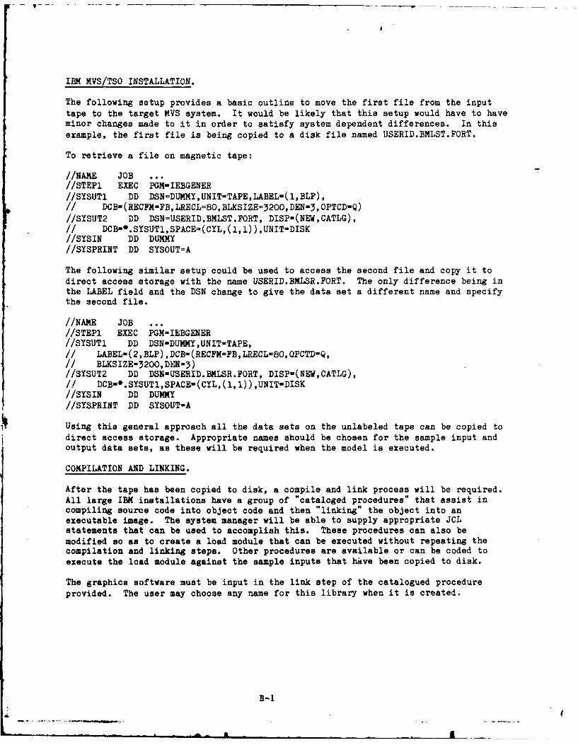
IBM MVS/TSO INSTALLATION.

The following setup provides a basic outline to move the first file from the inputtape to the target MVS system. It would be likely that this setup would have to haveminor changes made to it in order to satisfy system dependent differences. In thisexample, the first file is being copied to a disk file named USERID.BMLST.FORT.

To retrieve a file on magnetic tape:

//NAME JOB ...//STEPl EXEC PGM-IEBGENER//SYSUT1 DD DSN=DUMMY,UNIT=TAPE,LABEL=(1,BLP),// DCB=(RECFM=FB,LRECL=80,BLKSIZE=3200,DEN=3,OPTCD=Q)

//SYSUT2 DD DSN=USERID.BMLST.FORT, DISP=(NEW,CATLG),// DCB=*.SYSUTI,SPACE-(CYL,(1,1)),UNIT-DISK//SYSIN DD DUMMY//SYSPRINT DD SYSOUT=A

The following similar setup could be used to access the second file and copy it todirect access storage with the name USERID.BMLSR.FORT. The only difference being inthe LABEL field and the DSN change to give the data set a different name and specifythe second file.

//NAME JOB ...

//STEPI EXEC PGM=IEBGENER//SYSUTl DD DSN-DUMMY,UNIT=TAPE,// LABEL'(2,BLP),DCB=(RECFM=FB,LRECL-80, OPCTD-Q,// BLKSIZE=3200,DEN=3)//SYSUT2 DD DSN=USERID.BMLSR.FORT, DISP=(NEW,CATLG),// DCB=*.SYSUTI,SPACE=(CYL,(l,1)),UNIT-DISK//SYSIN DD DUMMY//SYSPRINT DD SYSOUT-A

Using this general approach all the data sets on the unlabeled tape can be copied todirect access storage. Appropriate names should be chosen for the sample input andoutput data sets, as these will be required when the model is executed.

COMPILATION AND LINKING.

After the tape has been copied to disk, a compile and link process will be required.All large IBM installations have a group of "cataloged procedures" that assist incompiling source code into object code and then "linking" the object into anexecutable image. The system manager will be able to supply appropriate JCLstatements that can be used to accomplish this. These procedures can also bemodified so as to create a load module that can be executed without repeating thecompilation and linking steps. Other procedures are available or can be coded to

execute the load module against the sample inputs that have been copied to disk.

The graphics software must be input in the link step of the catalogued procedure

provided. The user may choose any name for this library when it is created.

B-i

-- ........

APPENDIX C

DEC/VAX 11/750/780 INSTALLATIONS

DIGITAL EQUIPMENT CORP. (DEC) VAX 11/780/50; MICROVAX II.

After logging into the VAX, create a directory in your USER ID to hold the source

code from the tape. Assuming your USER ID is "PAULA" then, at the $ prompt, type:

$ CREATE/DIRECTORY [PAULA.MODEL]

Then make this your "default directory" with:

$ SET DEFAULT [PAULA.MODEL]

Next reserve a tape drive for the transmittal tape with:

$ ALLOCATE MT:

The name NT: is the device name of the tape drive you want to use. It may be

different on your installation - check with the system administrator. Use whatevername is suggested instead of MT: here and anywhere else MT: appears in thisdiscussion.

At this point you must physically mount the tape on the drive. Do NOT put a "write

ring" in the tape. That will safeguard the data on the tape from accidentalerasure. Some tape drives allow you to take the same precaution with push buttons onthe front panel.

Next mount the volume with:

$ NOUNT/FOREIGN/NOWRITE/BLOCK=32OO/DENSITY=I6OO/RECORD=80 MT:

Next copy the first file (which contains source code) to disk by typing:

$ COPY MT: BMLST.FOR

Copy the second file in the same way just use a different name:

$ COPY MT: BMLSR.FOR

Next copy the two plotting source files with:

i COPY NT: BPLOTT.FORCOPY MT: BPLOTR.FOR

Next copy the input files to disk by a series of copies like:

$ COPY MT: INPUTi$ COPY NT: INPUT2C OPY MT: INPUT3COPY MT: INPUT4

$ COPY MT: INPUT5

Enter as many copy commands as necessary to retrieve all the input data sets. If the

distribution notes specify, copy all succeeding files to disk choosing appropriatenames for the files.

C-i

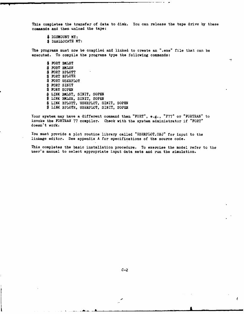
This completes the transfer of data to disk. You can release the tape drive by thesecommands and then unload the tape:

$ DISMOUNT KT:$ DEALLOCATE MT:

The programs must now be compiled and linked to create an ".exe" file that can beexecuted. To compile the programs type the following commands:

$ FORT B-LSTF PORT BNLSRFORT BPLOTTFORT BPLOTRFORT USERPLOTF ORT SINITFORT SOPENLINK BLST, SINIT, SOPENLINK BMLSR, SINIT, SOPN

I LINK BPLOTT, USERPLOT, SINIT, SOPENLINK BPLOTR, USERPLOT, SINIT, SOPEN

Your system may have a different command than "FORT", e.g., "F77" or "FORTRAN" toinvoke the FORTRAN 77 compiler. Check with the system administrator if "FORT"

doesn't work.

You must provide a plot routine library called "USERPLOT.OBJ" for input to the

linkage editor. See appendix A for specifications of the source code.

This completes the basic installation procedure. To exercise the model refer to theuser's manual to select appropriate input data sets and run the simulation.

C-2

-'L

APPENDIX D

UNIX SYSTEM V SYSTEMS INSTALLATIONS

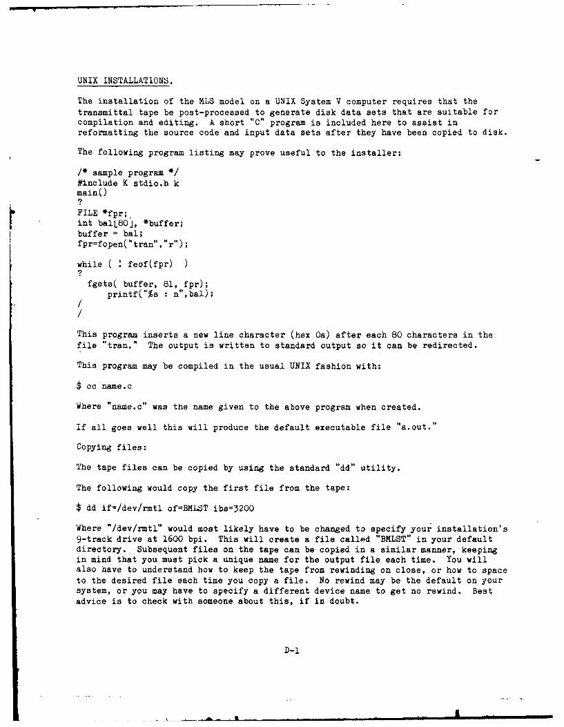
UNIX INSTALLATIONS.

The installation of the MLS model on a UNIX System V computer requires that thetransmittal tape be post-processed to generate disk data sets that are suitable forcompilation and editing. A short "C" program is included here to assist inreformatting the source code and input data sets after they have been copied to disk.

The following program listing may prove useful to the installer:

/* sample program#include K stdio.h kmain()

FILE *fpr;int balL80j, *buffer;buffer = bal;fpr=fopen("tran","r");

while ( feof(fpr) )?

fgets( buffer, 81, fpr);

printf("%s : n",bal);//

This program inserts a new line character (hex Oa) after each 80 characters in the

file "tran." The output is written to standard output so it can be redirected.

This program may be compiled in the usual UNIX fashion with:

$ cc name.c

Where "name.c" was the name given to the above program when created.

If all goes well this will produce the default executable file "a.out."

Copying files:

The tape files can be copied by using the standard "dd" utility.

The following would copy the first file from the tape:

$ dd if=/dev/rmtl of=BMLST ibs=3200

Where "/dev/rmtl" would most likely have to be changed to specify your installation's9-track drive at 1600 bpi. This will create a file called "BMLST" in your defaultdirectory. Subsequent files on the tape can be copied in a similar manner, keepingin mind that you must pick a unique name for the output file each time. You willalso have to understand how to keep the tape from rewinding on close, or how to spaceto the desired file each time you copy a file. No rewind may be the default on yoursystem, or you may have to specify a different device name to get no rewind. Best

advice is to check with someone about this, if in doubt.

D-1

. . .. I f • m - m m m m m ) • m m O I |I ni

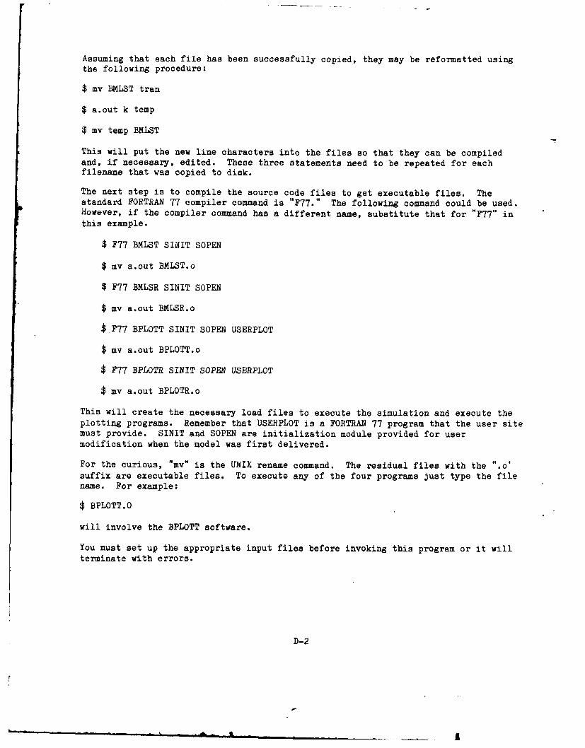
Assuming that each file has been successfully copied, they may be reformatted usingthe following procedure:

$ my BMLST tran

$ a.out k temp

$ my temp BMLST

This will put the new line characters into the files so that they can be compiledand, if necessary, edited. These three statements need to be repeated for eachfilename that vas copied to disk.

The next step is to compile the source code files to get executable files. Thestandard FORTRAN 77 compiler command is "F77." The following command could be used.However, if the compiler command has a different name, substitute that for "F77" inthis example.

$ F77 BMLST SINIT SOPEN

$ my a.out BMLST.o

$ F77 BMLSR SINIT SOPEN

$ mv a.out BMLSR.o

$F77 BPLOTT SINIT SOPEN USERPLOT

$ my a.out BPLOTT.o

$ F77 BPLOTR SINIT SOPEN USERPLOT

$ my a.out BPLOTR.o

This will create the necessary load files to execute the simulation and execute theplotting programs. Remember that USERPLOT is a FORTRAN 77 program that the user sitemust provide. SINIT and SOPEN are initialization module provided for usermodification when the model was first delivered.

For the curious, "mv" is the UNIX rename command. The residual files with the ".o'suffix are executable files. To execute any of the four programs just type the filename. For example:

$ BPLOTT.O

will involve the BPLOTT software.

You must set up the appropriate input files before invoking this program or it will

terminate with errors.

D-2

-- - " "" ' -mJ~mmuummmmmmmuunmmA

LIJ~