18 IEEE TRANSACTIONS ON PATTERN ANALYSIS AND …nicolas/publications/anomaly/pami_anomaly.pdf ·...

Anomaly Detection and Localizationin Crowded Scenes

Weixin Li, Student Member, IEEE, Vijay Mahadevan, Member, IEEE, and

Nuno Vasconcelos, Senior Member, IEEE

Abstract—The detection and localization of anomalous behaviors in crowded scenes is considered, and a joint detector of temporal

and spatial anomalies is proposed. The proposed detector is based on a video representation that accounts for both appearance and

dynamics, using a set of mixture of dynamic textures models. These models are used to implement 1) a center-surround discriminant

saliency detector that produces spatial saliency scores, and 2) a model of normal behavior that is learned from training data and

produces temporal saliency scores. Spatial and temporal anomaly maps are then defined at multiple spatial scales, by considering the

scores of these operators at progressively larger regions of support. The multiscale scores act as potentials of a conditional random

field that guarantees global consistency of the anomaly judgments. A data set of densely crowded pedestrian walkways is introduced

and used to evaluate the proposed anomaly detector. Experiments on this and other data sets show that the latter achieves state-of-

the-art anomaly detection results.

Index Terms—Video analysis, surveillance, anomaly detection, crowded scene, dynamic texture, center-surround saliency

Ç

1 INTRODUCTION

SURVEILLANCE video is extremely tedious to monitor whenevents that require follow-up have very low probability.

For crowded scenes, this difficulty is compounded by thecomplexity of normal crowd behaviors. This has motivated asurge of interest in anomaly detection in computer vision[1], [2], [3], [4], [5], [6], [7], [8], [9]. However, this effort ishampered by general difficulties of the anomaly detectionproblem [10]. One fundamental limitation is the lack of auniversal definition of anomaly. For crowds, it is alsoinfeasible to enumerate the set of anomalies that are possiblein a given surveillance scenario. This is compounded by thesparseness, rarity, and discontinuity of anomalous events,which limit the number of examples available to train ananomaly detection system.

One common solution to these problems is to defineanomalies as events of low probability with respect to aprobabilistic model of normal behavior. This enables astatistical treatment of anomaly detection, which conformswith the intuition of anomalies as events that deviate fromthe expected [10]. However, it introduces a number ofchallenges. First, it makes anomalies dependent on the scaleat which normalcy is defined. A normal behavior at a finevisual scale may be perceived as highly anomalous when alarger scale is considered, or vice versa. Hence, normalcy

models must be defined at multiple scales. Second, differenttasks may require different models of normalcy. For instance, adetector of freeway speed limit violations will rely onnormalcy models based on speed features. On the otherhand, appearance is more important for the detection ofcarpool lane violators, i.e., single-passenger vehicles incarpool lanes. Third, crowded scenes require normalcymodels robust to complex scene dynamics, involving manyindependently moving objects that occlude each other incomplex ways, and can have low resolution.

In result, anomaly detection can be extremely challen-ging. While this has motivated a great diversity of solutions,it is usually quite difficult to objectively compare differentmethods. Typically, these combine different representationsof motion and appearance with different graphical modelsof normalcy, which are usually tailored to specific scenedomains. Abnormalities are themselves defined in a some-what subjective form, sometimes according to what thealgorithms can detect. In some cases, different authors evendefine different anomalies on common data sets. Finally,experimental results can be presented on data sets of verydifferent characteristics (e.g., traffic intersection versussubway entrance), frequently proprietary, and with widelyvarying levels of crowd density.

In this work, we propose an integrated solution to allthese problems. We start by introducing normalcy modelsthat jointly account for the appearance and dynamics of complexcrowd scenes. This is done by resorting to a videorepresentation based on dynamic textures (DTs) [11]. Thisrepresentation is then used to design models of normalcyover both space and time. Temporal normalcy is modeledwith a mixture of DTs [12] (MDT) and enables the detectionof behaviors that deviate from those observed in the past.Spatial normalcy is measured with a discriminant saliencydetector [13] based on MDTs, enabling the detection ofbehaviors that deviate from those of the surroundingcrowd. The integration of spatial and temporal normalcy

18 IEEE TRANSACTIONS ON PATTERN ANALYSIS AND MACHINE INTELLIGENCE, VOL. 36, NO. 1, JANUARY 2014

. W. Li and N. Vasconcelos are with the Electrical and ComputerEngineering Department, University of California, San Diego, 9500Gilman Drive, La Jolla, CA 92093.E-mail: {wel017, nvasconcelos}@ucsd.edu.

. V. Mahadevan is with Yahoo! Labs, Embassy Golf Links Business Park,Bengaluru 560071, India. E-mail: [email protected].

Manuscript received 15 Apr. 2012; revised 26 Feb. 2013; accepted 14 May2013; published online 12 June 2013.Recommended for acceptance by G. Mori.For information on obtaining reprints of this article, please send e-mail to:[email protected], and reference IEEECS Log NumberTPAMI-2012-04-0294.Digital Object Identifier no. 10.1109/TPAMI.2013.111.

0162-8828/14/$31.00 � 2014 IEEE Published by the IEEE Computer Society

with respect to either appearance or dynamics leads to aflexible model of normalcy, applicable to the detection ofanomalies of relevance to various surveillance tasks.

To address the scale problem, MDTs are learned atmultiple spatial scales. This is done with an efficienthierarchical model, where layers of MDTs with successivelylarger regions of video support are learned recursively. Thelocal measures of spatial and temporal abnormality are thenintegrated into a globally coherent anomaly map, byprobabilistic inference. This is implemented with a condi-tional random field (CRF), whose single-node potentials areclassifiers of local measures of spatial and temporalabnormality, collected over a range of spatial scales. Theyare complemented by a novel set of interaction potentials,which account for spatial and temporal context, andintegrate anomaly information across the visual field.

Finally, to address the difficulties of empirical evaluationof anomaly detectors on crowded scenes, we introduce adata set of video from walkways in the campus of Universityof California, San Diego (UCSD), depicting crowds ofvarying densities. The data set contains 98 video sequences,and five well-defined abnormal categories. These are not“synthetic,” or “staged,” but abnormal events that occurnaturally, for example, bicycle riders that cross pedestrianwalkways. Ground truth is provided for abnormal events,as well as a protocol to evaluate detection performance.

The remainder of the paper is organized as follows:Section 2 reviews previous work on anomaly detection incomputer vision. The problems of temporal and spatialanomaly detection in crowded scenes are discussed inSection 3. This is followed by the mathematical character-ization of multiscale anomaly maps in Section 4, and theproposed CRF for integration of spatial and temporalanomalies across different spatial scales in Section 5. Finally,an extensive experimental evaluation is discussed inSection 6 and some conclusions are presented in Section 7.

2 PRIOR WORK

Recent advances in anomaly detection address eventrepresentation and globally consistent statistical inference.Contributions of the first type define features and modelsfor the discrimination of normal and anomalous patterns.Models of normal and abnormal behavior are then learnedfrom training data, and anomalies detected with a mini-mum probability of error decision rule. Although there aresome exceptions [5], the distribution of abnormal patterns isusually assumed uniform, and abnormal events formulatedas events of low probability under the model of normalcy.

One intuitive representation for event modeling is basedon object trajectories. It is comprised of either explicitly orimplicitly segmenting and tracking each object in the scene,and fitting models to the resulting object tracks [14], [15],[16], [6], [17], [18]. While capable of identifying abnormalbehaviors of high-level semantics (e.g., unusual long-termtrajectories), these procedures are both difficult andcomputationally expensive for crowded or cluttered scenes.A number of promising alternatives, which avoid proces-sing individual objects, have been recently proposed. Theseinclude the modeling of motion patterns with histograms ofpixel change [5], histograms of optical flow [19], [8], [20], oroptical flow measures [3], [4], [17], [1]. Among these, [3]

models local optical flow with a mixture of probabilisticprincipal component analysis (PCA) models, [4] and [17]draw inspiration from classical studies of crowd behavior[21] to characterize flow with interaction features (e.g.,social force model), and [1] learns the representative flow ofgroups by clustering optical flow-based particle trajectories.

These approaches emphasize dynamics, ignoring anoma-lies of object appearance and, thus, anomalous behaviorwithout outlying motion. Optical flow, pixel changehistograms, or other classical background subtractionfeatures are also difficult to extract from crowded scenes,where the background is by definition dynamic, there arelots of clutter, and occlusions. More complete representa-tions account for both appearance and motion. For example,[2] models temporal sequences of spatiotemporal gradientsto detect anomalies in densely crowded scenes, [22] declaresas abnormal spatiotemporal patches that cannot be recon-structed from previous frames, and [23] pools appearanceand motion features over spatial neighborhoods, using adistance to the nearest spatially colocated feature vectoramong all training video clips, to quantify abnormality.

Object-based representations, based on location, blobshape, and motion [7] or optical flow magnitude, gradients,location, and scale [9], have also been proposed. Otherrepresentations include a bag-of-words over a set ofmanually annotated event classes [24]. Various methodshave also been used to produce anomaly scores. Whilesimple spatial filtering suffices for some applications [19],crowded scenes require more sophisticated graphicalmodels and inference. For example, [6] and [1] adoptGaussian mixture models (GMM) to represent trajectories ofnormal behavior. Cong et al. [8] and Zhao et al. [20] learn asparse basis and define unusual events as those that canonly be reconstructed with either large error or thecombination of a large number of basis vectors.

Contributions of the second type address the integrationof local anomaly scores, which can be noisy, into a globallyconsistent anomaly map. The authors of [2], [25], and [7]guarantee temporally consistent inference by modelingnormal temporal sequences with hidden Markov models(HMMs). While this enforces consistency along the tempor-al dimension, there have also been efforts to producespatially consistent anomaly maps. For example, latentDirichlet allocation (LDA) has been applied to force flowfeatures, in the model of spatial crowd interactions of [4].On the other hand, [5] and [3] rely on Markov random fields(MRF) to enforce global spatial consistency. In the realm ofsparse representations, [20] guarantees consistency ofreconstruction coefficients over space and time by inclusionof smoothness terms in the underlying optimizationproblem. Finally, [9] models object relationships, usingBayesian networks to implement occlusion reasoning.

It should be noted that most of these methods havenot been tested on the densely crowded scenes consid-ered in this work. It is unclear that many of them coulddeal with the complex motion and object interactionsprevalent in such scenes. Furthermore, while mostmethods include some mechanism to encourage spatialand temporal consistency of anomaly judgments (MRF,LDA, etc.), the underlying decision rule tends to be eitherpredominantly temporal (e.g., trajectories, GMMs, HMMs,or sparse representations learned over time) or spatial

LI ET AL.: ANOMALY DETECTION AND LOCALIZATION IN CROWDED SCENES 19

(e.g., interaction models) but is rarely discriminant withrespect to both space and time. This makes it difficult toinfer whether spatial or temporal modeling are criticallyimportant by themselves, or what benefits are gainedfrom their joint modeling. Furthermore, the role of scaleis rarely considered. These issues motivate the contribu-tions of the following sections.

3 ANOMALY DETECTION

We start by proposing an anomaly detector that accountsfor scene appearance and dynamics, spatial and temporalcontext, and multiple spatial scales.

3.1 Mathematical Formulation

A classical formulation of anomaly detection, which weadopt in this work, equates anomalies to outliers. Astatistical model pXðxxxxÞ is postulated for the distribution ofa measurement XXXX under normal conditions. Abnormalitiesare defined as measurements whose probability is below athreshold under this model. This is equivalent to a statisticaltest of hypotheses:

. H0: xxxx is drawn from pXðxxxxÞ;

. H1: xxxx is drawn from an uninformative distributionpXðxxxxÞ / 1.

The minimum probability of error rule for this test is toreject the null hypothesis H0 if pXðxxxxÞ < �, where � is thenormalization constant of the uninformative distribution.As usual in the literature, we consider the problem ofanomaly detection from localized video measurements xxxx,where xxxx is a spatiotemporal patch of small dimensions.

3.2 Spatial versus Temporal Anomalies

The normalcy model pXðxxxxÞ can have both a temporal and aspatial component. Temporal normalcy reflects the intuitionthat normal events are recurrent over time, i.e., previousobservations establish a contextual reference for normalcyjudgments. Consider a highway lane where cars move witha certain orientation and speed. Bicycles or cars heading inthe opposite direction are easily identified as abnormalbecause they give rise to observations xxxx substantiallydifferent from those collected in the past. In this sense,temporal normalcy detection is similar to backgroundsubtraction [26]. A model of normal behavior is learnedover time, and measurements that it cannot explain aredenoted temporal anomalies.

Spatial normalcy reflects the intuition that some eventsthat would not be abnormal per se are abnormal within acrowd. Since the crowd places physical or psychologicalconstraints on individual behavior, behaviors feasible inisolation can have low probability in a crowd context. Forexample, while there is nothing abnormal about anambulance that rides at 50 mph in a stretch of highway,the same observation within a highly congested highway isabnormal. Note that the only indication of abnormality isthe difference between the crowd and the object at the time ofthe observation, not that the ambulance moves at 50 mph.Since the detection of such abnormalities is mostly based onspatial context, they are denoted spatial anomalies. Theirdetection does not depend on memory. Instead, it is basedon a continuously evolving, instantaneously adaptive,

definition of normalcy. In this sense, the detection of spatialanomalies can be equated to saliency detection [27].

3.3 Roles of Crowds and Scale

Most available background subtraction and saliency detec-tion solutions are not applicable to crowded scenes, wherebackgrounds can be highly dynamic. In this case, it is notsufficient to detect variations of image intensity, or evenoptical flow, to detect anomalous events. Instead, normalcymodels must rely on sophisticated joint representations ofappearance and dynamics. In fact, even such models can beineffective. Since crowds frequently contain distinct sub-entities, for example, vehicles or groups of people movingin different directions, anomaly detection requires model-ing multiple video components of different appearance anddynamics. A model that has been shown successful in thiscontext is the mixture of DTs [12]. This is the representationadopted in this work.

Another challenging aspect of anomaly detection withincrowds is scale. Spatial anomalies are usually detected atthe scale of the smallest scene entities, typically people.However, a normal event at this scale may be anomalous ata larger scale, and vice versa. For example, while a childthat rides a bicycle appears normal within a group ofbicycle riding children, the group is itself anomalous in acrowded pedestrian sidewalk. Local anomaly detectors,with small regions of interest, cannot detect such anomalies.To address this, we represent crowded scenes with ahierarchy of MDTs that cover successively larger regions.This is done with a computationally efficient hierarchicalmodel, where MDT layers are estimated recursively.

A similar challenge holds for temporal anomalies. Whiletheir detection is usually based on a small number of videoframes, certain anomalies can only be detected over longtime spans. For example, while it is normal for twopedestrian trajectories to converge or diverge at any pointin time, a cyclical convergence and divergence is probablyabnormal. Anomaly detection across time scales is, how-ever, more complex than across spatial scales, due toconstraints of instantaneous detection and implementationcomplexity. Since video has to be buffered before anomaliescan be detected, large temporal windows imply longdetection delays and storage of many video frames. Dueto this, we do not consider multiple temporal scales in thiswork. A single scale is chosen, using acceptable values ofdelay and storage complexity, and used throughout ourexperiments. Note that, like their spatial counterparts,temporal anomaly maps are computed at multiple spatialscales. Hence, in what follows, the term “scale” refers to thespatial support of anomaly detection, for both spatial andtemporal anomalies.

4 NORMALCY AND ANOMALY MODELING

In this section, we review the MDT model, discuss thedesign of temporal and spatial models of normalcy, andformulate the computation of anomaly maps.

4.1 Mixture of Dynamic Textures

The MDT models a sequence of � video frames xxxx1:� ¼½xxxx1; xxxx2; . . . ; xxxx� � as a sample from one of K dynamictextures [11]:


pðxxxx1:� Þ ¼XKi¼1

�ipðxxxx1:� jz ¼ iÞ: ð1Þ

The mixture components pðxxxx1:� jz ¼ iÞ are linear dynamicsystems (LDS) defined by

sssstþ1 ¼ Azsssst þ nnnnt; ð2aÞxxxxt ¼ Czsssst þmmmmt; ð2bÞ

�

where Z is a multinomial random variable of parameters ��ð�i � 0;

Pi �i ¼ 1Þ, which indexes the mixture component

from which xxxxt is drawn. sssst is a hidden state variable thatencodes scene dynamics, and xxxxt the vector of pixels in videoframe t. Az; Cz are the transition and observation matricesof component z, whose initial condition is ssss1 � Nð��z; SzÞ,and noise processes are defined by nnnnt � Nð0; QzÞ andmmmmt � Nð0; RzÞ. The model parameters are learned bymaximum-likelihood estimation (MLE) from a collectionof video patches, with the expectation-maximization (EM)algorithm of [12], which is reviewed in Appendix A.1,which is available in the Computer Society Digital Libraryat http://doi.ieeecomputersociety.org/10.1109/TPAMI.2013.111.

4.2 Temporal Anomaly Detection

Temporal anomaly detection is inspired by the popularbackground subtraction method of [26]. This uses a GMMper image location to model the distribution of imageintensities. Observations of low probability under theseGMMs are declared foreground. For anomaly detection incrowds, the GMM is replaced by an MDT, and the pixel gridreplaced by one of preset displacement. Grid locations definethe center of video cells, from which video patches areextracted. The patches extracted from a subregion (group ofcells) are used to learn an MDT, during a training phase, asillustrated in Fig. 1. After this phase, subregion patches oflow probability under the associated MDT are consideredanomalies. Given patch xxxx1:� , the distribution of the hiddenstate sequence ssss�1 under the ith DT component, pSjXðssss1:� jxxxx1:� ;z ¼ iÞ, is estimated with a Kalman filter and smoother [28],[29], as discussed in Appendix A.2, available in the onlinesupplemental material. The value of the temporal anomaly

map at location l is the negative-log probability of the most-likely state sequence for the patch at l:

T ðlÞ ¼ � logXKi¼1

�ip�ssssfig1:� ðlÞjz ¼ i

�" #; ð3Þ

where ssssfig1:� ðlÞ ¼ argmaxssss1:�

pðssss1:� jxxxx�ðlÞ; z ¼ iÞ. We note thatthis generalizes the mixture of PCA models of optical flow[3]. The matrix Cz of (2b) is a PCA basis for patches drawnfrom mixture component z, but the PCA decompositionreports to patch appearance, not optical flow. Patch dynamicsare captured by the hidden state sequence ssss1:� , which is atrajectory in PCA space. Hence, unlike mixtures of opticalflow, the representation is temporally smooth. The jointrepresentation of appearance and dynamics makes theMDT a better representation for crowd video than themixture of PCA.

4.3 Spatial Anomaly Detection

Spatial anomaly detection is inspired by previous work insaliency detection [27], [13]. Saliency is defined in a center-surround manner. Given a set of features, salient locationsare those of substantial feature contrast with their immedi-ate surround. Spatial anomalies are then defined aslocations whose saliency is above some threshold. In thiswork, we rely on the discriminant saliency criterion of [13].

4.3.1 Discriminant Saliency

Discriminant saliency formulates the saliency problem as ahypothesis test between two classes: a class of salient stimuli,and a background class of stimuli that are not salient. Twowindows are defined at each scene location l: a centerwindowW1

l , with label CðlÞ ¼ 1, containing the location, anda surrounding annular window W0

l , with label CðlÞ ¼ 0,containing background. A set of feature responses X arecomputed for each of the windows Wc

l , c 2 f0; 1g and SðlÞ,the saliency of location l, defined as the extent to which theydiscriminate between the two classes. This is quantified bythe mutual information (MI) between feature responses andclass label [13]:

SðlÞ ¼X1

c¼0

fpCðlÞðcÞKL½pXjCðlÞðxxxxjcÞkpXðxxxxÞ�g; ð4Þ

where pXjCðlÞðxxxxjcÞ are class-conditional densities and

KLðp qk Þ ¼RX pXðxxxxÞ log pXðxxxxÞ

qXðxxxxÞ dxxxx the Kullback-Leibler (KL)

divergence between pXðxxxxÞ and qXðxxxxÞ [30].Locations of maximal saliency are those where the

discrimination between center and surround can be madewith highest confidence, i.e., where (4) is maximal.The discriminant saliency principle can be applied to manyfeatures [31]. When X consists of optical flow, it generalizesthe force flow model of [4], where saliency is defined as thedifference between the optical flow at l and the averageflow in its neighborhood (see [4, (8)]). This is a simplifiedform of discriminant saliency, which replaces the MI of (4)by a difference to the mean background response.

4.3.2 Center-Surround Saliency with MDTs

Optical flow methods provide a coarse representation ofdynamics and ignore appearance. For background subtrac-tion, this problem has been addressed with the combinationof DTs and discriminant saliency [32]. While using a more


Fig. 1. Temporal anomaly detection. An MDT is learned per scenesubregion, at training time. A temporal anomaly map is produced bymeasuring the negative log probability of each video patch under theMDT of the corresponding region.

powerful representation than force flow, this method learnsa single DT from both center and surround windows. Thisassumes a homogeneity of appearance and dynamicswithin the two windows that do not hold for crowds,where foregrounds and backgrounds can be quite diverse.

In this work, we adopt the MDT as the probabilitydistribution pXjCðlÞðxxxx1:� jcÞ from which spatiotemporalpatches xxxx�1 are drawn. We note that under assumptions ofGaussian initial conditions and noise, patches xxxx1:� drawnfrom a DT have a Gaussian probability distribution [33],

xxxx1:� � Nð��;�Þ; ð5Þ

whose parameters follow from those of the LDS (2). Whenthe class-conditional distributions of the center and sur-round classes, c 2 f0; 1g, at location l are mixtures ofKc DTs, it follows that

pXjCðlÞðxxxx1:� jcÞ ¼XKc

i¼1

�ciN�xxxx1:� ; ��

ci ;�

ci

�

¼XKc

i¼1

�cipiXjCðlÞðxxxx1:� jcÞ;

ð6Þ

for c 2 f0; 1g. The marginal distribution is then

pXðxxxx1:� Þ ¼X1

c¼0

½pCðlÞðcÞpXjCðlÞðxxxx1:� jcÞ�

¼X1

c¼0

�pCðlÞðcÞ

XKc

i¼1

�ciN�xxxx1:� ; ��

ci ;�

ci

��

¼XK0þK1

i¼1

!iNðxxxx1:� ; ��i;�iÞ

¼XK0þK1

i¼1

!ipiXðxxxx1:� Þ;

ð7Þ

and the saliency measure of (4) requires the KL divergence

between (6) and (7). This is problematic because there is noclosed form solution for the KL divergence between two

MDTs. However, because the MDT components areGaussian, it is possible to rely on popular approximations

to the KL divergence between Gaussian mixtures. We adoptthe variational approximation of [34]:

KLðpXjCkpXÞ

�Xi

�Ci log

PKCj �Cj exp

��KL

�piXjC

��pjXjC��PK0þK1

j !j exp��KL

�piXjC

��pjX��( )

:ð8Þ

Each term of (8) contains a KL divergence between DTs,

which can be computed in closed form [35]. For example,for the terms in the denominator

KL�piXjC

��pjX�¼ 1

2logj�jj��Ci ��þ Tr

��1j �Ci

�þ��Ci � ��j��2

�j�m�

" #;ð9Þ

where m is the number of pixels per frame, andkzzzzk� ¼ zzzzT��1zzzz. Numerator terms are computed similarly.

All computations can be performed recursively [35].

4.3.3 Spatial Anomaly Map

The spatial anomaly map is a map of the saliency SðlÞ atlocations l. Given a location, this requires 1) learning MDTsfrom center and surround windows, and 2) computing aweighted average of these mixtures to obtain (7). Sincelearning MDTs per location is computationally prohibitive,we resort to the following approximation. A dense collec-tion of overlapping spatiotemporal patches is first extractedfrom VðtÞ, a 3D video volume temporally centered at thecurrent frame. A single MDT with Kg mixture components,denoted f��gi ;�

gigKg

i¼1, is learned from this patch collection.Each patch is then assigned to the mixture component oflargest posterior probability. This segments the volume intosuperpixels, as shown in Fig. 2.

At location l, the MDTs of (6) and (7) are derived fromthe global mixture model. The DT components are assumedequal to those of the latter and only the mixing proportionsare recomputed, using the ratio of pixels assigned to eachcomponent in the respective windows:

pXjCðlÞðxxxx1:� jcÞ ¼XKg

i¼1

Pl2Wc

lMilP

l2Wcl1N�xxxx1:� ; ��

gi ;�

gi

�; ð10Þ

for c 2 f0; 1g. Mil ¼ 1 if l is assigned to mixturecomponent i and 0 otherwise. The prior probabilities forcenter and surround, pCðcÞ, are proportional to the ratio ofvolumes of center and surround windows. SðlÞ iscomputed with (4), using (8) and (9). Note that the KLdivergence terms in (8) only require the computation ofKg

2

� �KL divergences between the Kg mixture components,

and these are computed only once per frame because allmixture components are shared (i.e., the termsexp ð�KLðp qk ÞÞ in (8) are fixed per frame). This procedureis repeated for every frame in the test video, as illustratedin Fig. 2.

4.4 Multiscale Anomaly Maps

To account for anomalies at multiple spatial scales, we relyon a hierarchical mixture of dynamic textures (H-MDT).This is a model with various MDT layers, learned fromregions of different spatial support. At the finest scale, avideo sequence is divided into nL subregions (e.g., 5� 8


Fig. 2. Spatial anomaly detection using center-surround saliency withMDT models.

subregions). nL MDT models fMMMMignLi¼1 are then learned from

patches extracted from each of the subregions. At the

coarsest scale, the whole visual field is represented with a

global MDT. This results in a hierarchy of MDT models

ffMMMM1i gn1

i¼1; . . . ;MMMML1 g, where MMMMs

j , the jth model at scale s, is

learned from subregion Rsj . The hierarchy of support

windows ffR1i gn1

i¼1; . . . ;RLg resembles the spatial pyramid

structure of [36]. H-MDT models can be learned efficiently

with the hierarchical expectation-maximization (H-EM)

algorithm of [37]. Rather than collecting patches anew from

larger regions, it estimates the models at a given layer

directly from the parameters of the MDT models at the layer

of immediately higher resolution.For anomaly detection, each model is applied to the

corresponding window. This produces L anomaly maps,fT 1; . . . ; T Lg, as illustrated in Fig. 3. A hierarchy of spatialanomaly maps, fS1; . . . ;SLg is also computed. For all s, thecomputation of Ss relies on a global mixture model MMMM.The mixing proportions of (10) are computed usingsurround windows of size identical to fRs

ig and centerwindows of constant size, as summarized in Algorithm 1(see Appendix B for all algorithms, available in the onlinesupplemental material.

5 GLOBALLY CONSISTENT ANOMALY MAPS

In this section, we introduce a layer of statistical inference to

fuse anomaly information across time, space, and scale in a

globally consistent manner.

5.1 Discriminative Model

The anomaly maps of the previous section span space, time,

and spatial scale. Being derived from local measurements,

they can be noisy. A principled framework is required to

1) integrate anomaly scores from the individual maps,

2) eliminate noise, and 3) guarantee spatiotemporal con-

sistency of anomaly judgments throughout the visual field.

For this, we rely on a conditional random field [38] inspired

by the discriminative random field (DRF) of [39]. An

anomaly label yi 2 f�1; 1g is defined at each location i in a

set S of observation sites. Given a video clip xxxx, the

conditional likelihood of observing a configuration ofanomaly labels yyyy ¼ fyiji 2 Sg is

P ðyyyyjxxxxÞ ¼ 1

Zexp

(Xi2S

Aðyi; xxxxÞ

þXi2S

"1

jN ijXj2N i

Iðyi; yj; xxxx; i; jÞ#)

;

ð11Þ

where Z is a partition function and N i the neighborhood ofsite i. The single-site and interaction potentials of (11),

Aðyi; xxxxÞ ¼ log��yiwwww

Tffffi�; ð12Þ

where �ðxÞ ¼ ð1þ e�xÞ�1 is the sigmoid function, and

Iðyi; yj; xxxx; i; jÞ ¼ yiyj � vvvvT��ðffffi; ffffj; i; jÞ ð13Þ

are based on a feature vector ffffi that concatenates the spatialand temporal anomaly scores of site i at the L spatial scales,plus a bias term (set to 1):

ffffi ¼1; T 1ðiÞ; . . . ; T LðiÞ;S1ðiÞ; . . . ;SLðiÞ

T: ð14Þ

wwww; vvvv are parameter vectors and �� a compound feature:

��ðffffi; ffffj; i; jÞ ¼ e��ji�jj expð�hhhhi;jÞ; ð15Þ

where ji� jj is the euclidean distance between sites i; j, andexpð�hhhhi;jÞ the entry-wise exponential of �hhhhi;j. The vectorhhhhi;j contains the diagonal entries of ðffffi � ffffjÞðffffi � ffffjÞT .

The single-site potential of (12) reflects the anomalybelief at site i. Using it alone, i.e., without (13), (11) is alogistic regression model. In this case, the detection of eachanomaly is based on information from site i exclusively. Theaddition of the interaction potential of (13) enables themodel to take into account information from site i’sneighborhood N i. This smoothes the single-site prediction,encouraging consistency of neighboring labels. The inter-action potential can be interpreted as a classifier thatpredicts whether two neighboring sites have the samelabel. Note that because ffff contains anomaly scores atdifferent spatial scales, hhhhi;j (or ��i;j) accounts for the


Fig. 3. Computation of temporal anomaly maps with multiscale spatial supports using the H-MDT. MDTs of increasingly larger spatial support areestimated recursively, with the H-EM algorithm. Their application to a query video produces temporal anomaly maps based on supports of variousspatial scales.

similarity between the two observations in anomaly spacesof different scale (i.e., under different spatial normalcycontexts). The interaction potentials adaptively modulatethe intensity of intersite smoothing according to thesesimilarity measures (and how they are weighted by vvvv). Theparameters wwww and vvvv encode the relative importance ofdifferent features.

5.2 Online CRF Filter

The model of (11) requires inference over the entire videosequence. This is not suitable for online applications. Anonline version can be implemented by conditioning theanomaly label yyyyð�Þ at time � on 1) observations for t � , and2) anomaly labels for t < � , leading to

P�yyyyð�ÞjfyyyyðtÞg��1

t¼1 ; fxxxxðtÞg�t¼1; �

�¼ 1

Z exp

(Xi2S�

"A�yð�Þi ; xxxxð�Þ

�

þ 1

jN SSi j

Xj2N SS

i

ISS

�yð�Þi ; yj; xxxx

ð�Þ; i; j�

þ 1��N TTi

��Xk2N TT

i

ITT

�yð�Þi ; yk; xxxx; i; k

�#);

ð16Þ

where S� is the set of observations at time � (pixels of the

current frame). Two neighborhoods are defined per location

i: spatial N SSi (N SS

i S� ) and temporal N TTi (N TT

i fStg��1t¼1 ).

The graphical model is shown at the top of Fig. 4, and these

neighborhoods at the bottom. The parameters �� ¼fwwww; vvvvTT; vvvvSS; �TT; �SSg are estimated during training.

5.2.1 Learning

Both (11) and (16) can be learned with standard optimizationtechniques, such as gradient descent or the Broyden-Fletcher-Goldfarb-Shanno (BFGS) method. To improve generalization,the model is regularized with a Gaussian prior of standard

deviation , for all parameters. Given N independenttraining samples fxxxxðnÞ; yyyyðnÞgNn¼1, the gradients of the regular-ized log-likelihood with respect to wwww, vvvv, and � are

@

@wwwwlog��yyyyðnÞ�Nn¼1j�xxxxðnÞ

�Nn¼1

�¼XNn¼1

(Xi2S

�� yðnÞi wwwwTffff

ðnÞi

�yðnÞi ffff

ðnÞi

� IE

�Xi2S

�� yiwwwwTffffðnÞi

�yiffff

ðnÞi

�)� 1

2wwwwwwww;

ð17Þ

@

@vvvvlog p

��yyyyðnÞ�Nn¼1j�xxxxðnÞ

�Nn¼1

�¼XNn¼1

(Xi2S

�1

jN ijXj2N i

�e��ji�jjy

ðnÞi y

ðnÞj exp

��hhhhðnÞi;j

��

� IE

"Xi2S

1

jN ijXj2N i

�e��ji�jjyiyj exp

��hhhhðnÞi;j

��!#)� 1

2vvvvvvvv;

ð18Þ

and

@

@�log p

fyyyyðnÞgNn¼1

��fxxxxðnÞgNn¼1

�

¼XNn¼1

Xi2S

1

jN ijXj2N i

��I�yðnÞi ; y

ðnÞj ; xxxxðnÞ; i; j

�ji� jj

�8<:

þ IEXi2S

1

jN ijXj2N i

�Iðyi; yj; xxxxðnÞ; i; j

�ji� jj

�0@

1A

24

359=;� 1

2��;

ð19Þ

where the expectation is evaluated with distributionpðYjX; ��Þ. The conditional expectations of (17)-(19) requireevaluation of the partition function Z, a problem known tobe NP-hard. As is common in the literature, this difficulty isavoided by estimating expectations through sampling.Although sampling methods such as Markov chain MonteCarlo (MCMC) can converge to the true distribution, thisusually requires many iterations. Since the procedure mustbe repeated per gradient ascent step, these methods areimpractical. On the other hand, approximations such ascontrastive divergence minimization (which runs MCMC alimited number of times with specific starting points) havebeen shown to be successful for vision applications [40],[41]. We adopt these approximations for CRF learning.

This leverages the fact that, denoting any of theparameters wwww; vvvvTT; vvvvSS; �TT; �SS by , the partial gradients of(17)-(19) are

@

@log p

��yyyyðnÞ�Nn¼1j�xxxxðnÞ

�Nn¼1

; ��

¼XNn¼1

�F@�yyyyðnÞ; xxxxðnÞ

�� IEðYjX;��Þ

F@ðyyyy; xxxxðnÞÞ

�� 1

2;

ð20Þ

where F@ðyyyy; xxxxÞ is the sum of the terms in the summationsof (17), (18), or (19) that depend on . Contrastivedivergence approximates the intractable conditional


Fig. 4. CRF filter. Top: Graphical model. Bottom: Spatial and temporalneighborhoods.

expectation IEðYjX;�Þ½F@ðyyyy; xxxxðnÞÞ� by F@ðyyyy; xxxxðnÞÞ, where yyyy is

the “evil twin” of the ground-truth label field yyyyðnÞ [41]. yyyy is

drawn by MCMC, using the inference procedure discussed

in Section 5.2.2, the current parameter estimates, and the

ground-truth labels yyyyðnÞ as a starting point.Given the estimate of the partial gradients, the gradient

ascent rule for parameter updates reduces to

þ �XNn¼1

�F@�yyyyðnÞ; xxxxðnÞ

�� F@

�yyyyðnÞ; xxxxðnÞ

�� 1

2

" #;

ð21Þ

where � is a learning rate. In our implementation, this rule

is initialized with vvvvTT ¼ vvvvSS ¼ 1 and �TT ¼ �SS ¼ 0. The initial

value of wwww is learned, assuming a logistic regression model

(vvvvTT ¼ vvvvSS ¼ 0 in (16)), with the procedure of [43].

5.2.2 Inference

The inference problem is to determine the most likely

anomaly prediction yyyy? for a query frame xxxxð�Þ, given

previous predictions fyyyyðtÞg��1t¼1 , and observations fxxxxðtÞg�t¼1:

yyyy? ¼ argmaxyyyy

log p�yyyyj�yyyyðtÞ��1

t¼1;�xxxxðtÞ��t¼1

; ��

¼ argmaxyyyy

Xi2S

�A�yi; xxxx

ð�Þ�þ 1

jN ijXj2N i

Iðyi; yj; xxxx; i; jÞ�:

ð22Þ

Again, exact inference is intractable. We rely on Gibbs

sampling to approximate the optimal prediction. This

consists of drawing labels from the conditional distribution:

p�yij�xxxxðtÞ��t¼1;�yyyyðtÞ��1

t¼1; yyyy�i; �

�¼p�yi; yyyy�ij

�xxxxðtÞ��t¼1;�yyyyðtÞ��1

t¼1; ��

p�yyyy�ij

�xxxxðtÞ��t¼1;�yyyyðtÞ��1

t¼1; ��

¼ 1

Z�iexp

Fi��xxxxðtÞ��t¼1;�yyyyðtÞ��1

t¼1; yyyy�i; yi; �

�;

ð23Þ

where FiðfxxxxðtÞg�t¼1; fyyyyðtÞg��1t¼1 ; yyyy�i; yi; �Þ is the sum of poten-

tial functions that depend on site i (i.e., its “Markov

blanket”):

Fi��xxxxðtÞ��t¼1;�yyyyðtÞ��1

t¼1; yyyy�i; yi; �

�¼ A

�yi; xxxx

ð�Þ�þ 1

jN ijXj2N i

I�yi; yj;

�xxxxðtÞ��t¼1; i; j

�

þXj:i2N j

1

jN jjI�yj; yi;

�xxxxðtÞ��t¼1; j; i

�;

ð24Þ

and Z�i the corresponding partition function:

Z�i ¼Xy0i

exphFi��xxxxðtÞ��t¼1;�yyyyðtÞ��1

t¼1; yyyy�i; y

0i; �

�i: ð25Þ

The procedure is detailed in Algorithms 2 and 3, available

in the online supplemental material, where we present the

online CRF filter used to estimate the label field. During

learning, the filter is initialized with the ground-truth labels

(yyyy0 ¼ yyyyð�Þ). During testing, this initialization relies on the

predictions of the single-site classifiers (vvvvTT ¼ vvvvSS ¼ 0). In our

implementation, the filter is run for Ns ¼ 10 iterations.Again, the complete anomaly detection procedure issummarized in Algorithm 4, available in the onlinesupplemental material.

6 EXPERIMENTS

In this section, we introduce a new data set and anexperimental protocol for evaluation of anomaly detectionin crowded environments and use it to evaluate theproposed anomaly detector.

6.1 UCSD Pedestrian Anomaly Data Set

In the literature, anomaly detection has frequently beenevaluated by visual inspection [19], [7], [3], or with coarseground truth, for example, frame-level annotation ofabnormal events [4], [1]. This does not completely addressthe anomaly detection problem, where it is usually desiredto localize anomalies in both space and time. To enable this,we introduce a data set1 of crowd scenes with preciselylocalized anomalies and metrics for the evaluation of theirdetection. The data set consists of video clips recorded witha stationary camera mounted at an elevation, overlookingpedestrian walkways on the UCSD campus. The crowddensity in the walkways is variable, ranging from sparse tovery crowded. In the normal setting, the video containsonly pedestrians. Abnormal events are due to either 1) thecirculation of nonpedestrian entities in the walkways, or2) anomalous pedestrian motion patterns. Commonlyoccurring anomalies include bikers, skaters, small carts,and people walking across a walkway or in the surroundinggrass. A few instances of wheelchairs are also recorded. Allabnormalities occur naturally, i.e., they were not staged orsynthesized for data set collection.

The data set is organized into two subsets, correspondingto the two scenes of Fig. 5. The first, denoted “Ped1,”contains clips of 158� 238 pixels, which depict groups ofpeople walking toward and away from the camera, andsome amount of perspective distortion. The second,denoted “Ped2,” has spatial resolution of 240� 360 pixelsand depicts a scene where most pedestrians move horizon-tally. The video footage of each scene is sliced into clips of120-200 frames. A number of these (34 in Ped1 and 16 inPed2) are to be used as training set for the condition of


1. Available from http://www.svcl.ucsd.edu/projects/anomaly/data-set.html.

Fig. 5. Exemplar normal/abnormal frames in Ped1 (top) and Ped2(bottom). Anomalies (red boxes) include bikes, skaters, carts, andwheelchairs.

normalcy. The test set contains clips (36 for Ped1 and 12 forPed2) with both normal (around 5,500) and abnormal(around 3,400) frames. The abnormalities of each set aresummarized in Table 1.

Frame-level ground-truth annotation, indicating whetheranomalies occur within each frame, and manually collectedpixel-level binary anomaly masks, which identify the pixelscontaining anomalies, are available per test clip. We notethat this includes ground truth on Ped1 contributed byAnti�c and Ommer [9], and supersedes the ground truthavailable on an earlier version of this work [43]. We denotethe current ground truth by “full annotation” and theprevious one by “partial annotation.” Unless otherwisenoted, the results of the subsequent sections correspond tothe full annotation.

6.2 Evaluation Methodology

Two criteria are used to evaluate anomaly detectionaccuracy: a frame-level criterion and a pixel-level criterion.Both are based on true-positive rates (TPR) and false-positive rates (FPRs), denoting “an anomalous event” as“positive” and “the absence of anomalous events” as“negative.” A frame containing anomalies is denoted apositive, otherwise a negative. The true and false positivesunder the two criteria are:

. Frame-level criterion. An algorithm predicts whichframes contain anomalous events. This is comparedto the clip’s frame-level ground-truth anomalyannotations to determine the number of true- andfalse-positive frames.

. Pixel-level criterion. An algorithm predicts whichpixels are related to anomalous events. This iscompared to the pixel-level ground-truth anomalyannotation to determine the number of true-positiveand false-positive frames. A frame is a true positiveif 1) it is positive and 2) at least 40 percent of itsanomalous pixels are identified; a frame is a falsepositive if it is negative and any of its pixels arepredicated as anomalous.

The two measures are combined into a receiver operatingcharacteristic (ROC) curve of TPR versus FPR:

TPR ¼ # of true-positive frame

# of positive frame;

FPR ¼ # of false-positive frame

# of negative frame:

Performance is also summarized by the equal error rate(EER), the ratio of misclassified frames at whichFPR ¼ 1� TPR, for the frame-level criterion, or rate ofdetection (RD), i.e., 1-EER, for the pixel-level criterion.

Note that, although widely used in the literature, theframe-level criterion only measures temporal localizationaccuracy. This enables errors due to “lucky co-occurrences”of prediction errors and true abnormalities. For example, itassigns a perfect score to an algorithm that identifies asingle anomaly at a random location of a frame withanomalies. The pixel-level criterion is much stricter andmore rigorous. By evaluating both the temporal and spatialaccuracy of the anomaly predictions, it rules out these“lucky co-occurrences.” We believe that the pixel-levelcriterion should be the predominant criterion for evaluationof anomaly detection algorithms.

6.3 Experimental Setup

Unless otherwise noted, observation sites are a video sub-lattice with spatial interval of four pixels and temporalinterval of five frames. Temporal anomaly maps rely onpatches of 13� 13� 15 pixels. The temporal extent of15 frames provides a reasonable compromise between theability to detect anomalies and the delay (1.5 s) and storage(15 video frames) required for anomaly detection. Tominimize computation, patches of variance smaller than500 are discarded.2 Temporal H-MDT models are learnedfrom fine to coarse scale. At the finer scale, there are 6� 10windows R1

i on Ped1 (8� 11 for Ped2), each covering a41�41 pixel area and overlapping by 25 percent with eachof its four neighbors. An MDT of five components islearned per window. At coarser spatial scales, an MDT isestimated from the MDTs of the four regions that it coversat the immediately finer resolution. Each estimated MDThas one more component than its ancestor MDTs. Overall,there are 10 scales in Ped1 and 11 in Ped2. Spatial anomalymaps use a 31�31 center window and surround windowsof size equivalent to Rs

i . For segmentation, 7� 7� 10patches are extracted from the 40 frames surrounding thatunder analysis. There are five DT components at all levelsof the spatial hierarchy. Both temporal and spatial MDTshave an eight-dimensional state space. The sensitivity ofthe proposed detector to some of these parameters isdiscussed in Appendix C.2, available in the onlinesupplemental material.

6.4 Descriptor Comparison

The first experiment evaluated the benefits of MDT-basedover optical flow descriptors. The optical flow descriptorsconsidered were the local motion histogram (LMH) of [19],the force flow descriptor of [4], and the mixture of opticalflow models (MPPCA) of [3]. LMH uses statistics of localmotion, and is representative of traditional backgroundsubtraction representations, force flow is a descriptor forspatial anomaly detection, and MPPCA a temporalanomaly detector. For the MDT, only the anomaly mapsof finest temporal and coarsest spatial scale were con-sidered here. Since the goal was to compare descriptors,the high-level components of the models in which theywere proposed, for example, the LDA of [4], the MRF of[3], and the proposed CRF, were not used. Instead,anomaly predictions were smoothed with a simple


2. This variance threshold is quite conservative, only eliminating regionsof very little motion. For the data sets used in our experiments, this has notled to the elimination of any objects from further consideration. In othercontexts, for example, scenes where objects are static for periods of time,this could happen. In this case, the threshold should be set to zero.

TABLE 1Composition of UCSD Anomaly Data Set

anumber of clips/number of anomaly instances. b some clips containmore than one type of anomaly.

20� 20� 10 Gaussian filter. Anomaly predictions weregenerated by thresholding the filtered anomaly maps andROC curves by varying thresholds.

The performance of the different descriptors, under boththe frame-level (EER) and pixel-level (RD) criteria (usingboth full and partial annotation in Ped1), is summarized inTable 2. The corresponding ROC curves are presented inAppendix C.1 (Fig. 13), available in the online supplementalmaterial. Examples of detected anomalies are shown inFig. 6. Under the frame-level criterion, temporal MDT hasthe best performance in both scenes. Spatial MDT performsworse than others in Ped1 but ranks second in Ped2.However, for the more precise pixel-level criterion, spatialMDT is the top or second best performer. In this case, bothMDTs significantly outperform all optical flow descriptors.The gap between corresponding competitors (e.g., temporalMDT versus MPPCA or LMH, spatial MDT versus forceflow) is of at least 10 percent RD. These results show thatthere is a definite benefit to the joint representation ofappearance and dynamics of the MDT.

This is not totally surprising, given the limitations ofoptical flow. First, the brightness constancy assumption iseasily violated in crowded scenes, where stochastic motionand occlusions prevail. Second, optical flow measuresinstantaneous displacement, while the DT is a smoothmotion representation with extended temporal support.Finally, while optical flow is a bandpass measure, whicheliminates most of the appearance information, the DTmodels both appearance and dynamics. The last twoproperties are particularly important for crowded scenes,where objects occlude and interact in complicated manners.

Overall, although optical flow can signal fast movinganomalous subjects, it leads to too many false positives inregions of complex motion, occlusion, and so on. Moreinteresting is the lack of advantage for either spatial ortemporal anomaly detection, both among MDT maps andprior techniques (no clear advantage to either force flow orMPPCA). In fact, as shown in Fig. 6, temporal and spatialanomalies tend to be different objects. This suggests thecombination of the two strategies.

6.5 Scale and Globally Consistent Prediction

We next investigated the benefits of information fusionacross space and scale, with the proposed CRF. We startedwith a single-scale description (S-MDT), using only theanomaly maps at finest temporal and coarsest spatialscales, i.e., a 3D feature per site. We next considered amultiscale description, using the whole H-MDT. In bothcases, inference was performed with logistic regression, i.e.,the interaction term of (16) turned off, and the Gaussianfilter of the previous section. In each trial, the logisticclassifier was trained by Newton’s method [42]. Finally, weconsidered the full blown CRF, denoted CRF filter. Thedimensions of the spatial and temporal CRF neighborhoodswere set to jN SSj ¼ 6, jN TTj ¼ 3. ROC curves were generatedby varying the threshold for prediction.

Table 3 presents a comparison of the three approaches.The corresponding ROC curves are shown in Appendix C.1(Fig. 14), available in the online supplemental material.Under the pixel-level criterion, the multiscale maps havehigher accuracy than their single-scale counterparts, demon-strating the benefits of modeling anomalies in scale space(improvement of RD by as much as 11 percent). The CRF


TABLE 2Descriptor Performance on UCSD Anomaly Data Set

�numbers outside/inside parentheses are results by full/partial annota-tion (same for the rest of the paper).

TABLE 3Filter Performance on the UCSD Anomaly Data Set

Fig. 6. Anomaly predictions of temporal MDT, spatial MDT, MPPCA, force flow, and LMH (from left to right). Red regions are abnormal pixels. Allpredictions generated with thresholds such that the different approaches have similar FPR under frame-level protocol (these settings apply to all thesubsequent figures unless otherwise stated).

filter further improves performance (improvement of RD byas much as 3 percent), demonstrating the gains of globallyconsistent inference. As shown in Fig. 7, the visual improve-ments are even more substantial.3 Simple filtering does nottake into account interactions between neighboring sites andsmooths the anomaly maps uniformly. On the other hand,the CRF adapts the degree of smoothing to the spatiotem-poral structure of the anomalies, increasing the precision ofanomaly localization. Note how, in Fig. 7, the CRF-filtersuccessfully excludes occluded but normally behavingpedestrians from anomaly regions. These improvementsare not always captured by the frame-level criterion. In fact,there is little EER difference between S-MDT and H-MDT.The inconsistency between frame- and pixel-level results inTables 2 and 3 shows that the former is not a good measure ofanomaly detection performance. Henceforth, only the pixel-level criterion is used in the remaining experiments on thisdata set.

6.6 Anomaly Detection Performance

We next evaluated the performance of the completeanomaly detector. For this, we selected two detectorsfrom the recent literature, with state-of-the-art perfor-mance for temporal [8] and combined spatial andtemporal anomaly detection [9]. The RD of the variousmethods is summarized in Table 4, for both partial andfull annotation. The corresponding ROC curves are shownin Fig. 8. Table 4 also presents the processing time pervideo frame of each method. Missing entries indicateunavailable results for the particular data set and/orannotation type. A discussion of the detection errors madeby the detector is given in Appendix C.3, available in theonline supplemental material.

On Ped1, the temporal component of the proposeddetector substantially outperforms the temporal detector of[8]. A multiple-scale temporal anomaly map with CRFfiltering increases the 46 percent RD4 of [8] to 52 percent.A similar implementation of the spatial anomaly detector(a multiple-scale map plus CRF filtering) achieves 58 percent.Combining both maps and multiple spatial scales further

improves the RD to 65 percent. Computationally, theproposed detector is also much more efficient. Forimplementations on similar hardware (see footnotesof Table 4), it requires 1.11 s/frame, as compared to the

3.8 s/frame reported for [8].Like the proposed detector, the Bayesian video parsing

(BVP) of [9] combines spatial and temporal anomalydetection, using a more complex video representation,parsing of the video to extract all the objects in the scene,a support vector machine classifier for detection of temporalanomalies, a graphical model with seven nodes per site

(and multiple nonparametric models for location, scale, andvelocity) for detection of spatial anomalies, and occlusionreasoning. This is an elegant solution, which achievesslightly better RD than the proposed detector (2 percent forfull and 3 percent for partial annotation), but at substan-

tially higher computational cost (5 to 10 times slower). Webelieve that when both accuracy and computation areconsidered, the proposed detector is a more effectivesolution. However, these results suggest that gains could

be achieved by expanding the proposed CRF, as [9] trades amuch simpler representation of video dynamics (opticalflow versus MDT) for more sophisticated inference. It wouldbe interesting to consider CRF extensions with some of theproperties of the graphical model of [9], namely, explicit

occlusion reasoning. This is left for subsequent research.


TABLE 4Performance of Various Methods (RD/Seconds per Frame) by Pixel-Level Criterion on UCSD Anomaly Data Set

Implementation: } C/2.8-GHz CPU/2-GB RAM; \ C++ and Matlab (feature extraction and model inference)/2.6GHz CPU/2GB RAM; #Matlab/dual-core 2.7GHz CPU/8GB RAM.

Fig. 7. Examples of anomaly localization with Gaussian smoothing (in blue) and CRF filter (in red). The latter predicts more accurately thespatiotemporal support of anomalies in crowded regions, where occlusion is prevalent.

Fig. 8. ROC curves of pixel-level criterion on Ped1.

3. More results at http://www.svcl.ucsd.edu/projects/anomaly/results.html.

4. These numbers refer to partial annotation, the only available for [8].

6.7 Role of Context in Anomaly Judgments

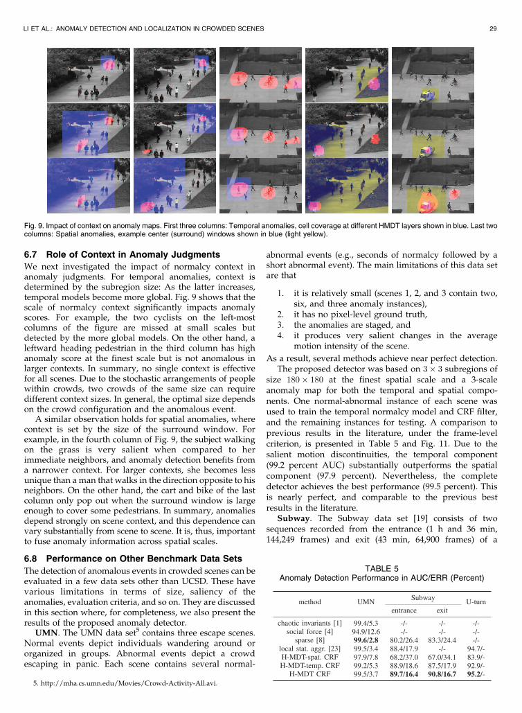
We next investigated the impact of normalcy context inanomaly judgments. For temporal anomalies, context isdetermined by the subregion size: As the latter increases,temporal models become more global. Fig. 9 shows that thescale of normalcy context significantly impacts anomalyscores. For example, the two cyclists on the left-mostcolumns of the figure are missed at small scales butdetected by the more global models. On the other hand, aleftward heading pedestrian in the third column has highanomaly score at the finest scale but is not anomalous inlarger contexts. In summary, no single context is effectivefor all scenes. Due to the stochastic arrangements of peoplewithin crowds, two crowds of the same size can requiredifferent context sizes. In general, the optimal size dependson the crowd configuration and the anomalous event.

A similar observation holds for spatial anomalies, wherecontext is set by the size of the surround window. Forexample, in the fourth column of Fig. 9, the subject walkingon the grass is very salient when compared to herimmediate neighbors, and anomaly detection benefits froma narrower context. For larger contexts, she becomes lessunique than a man that walks in the direction opposite to hisneighbors. On the other hand, the cart and bike of the lastcolumn only pop out when the surround window is largeenough to cover some pedestrians. In summary, anomaliesdepend strongly on scene context, and this dependence canvary substantially from scene to scene. It is, thus, importantto fuse anomaly information across spatial scales.

6.8 Performance on Other Benchmark Data Sets

The detection of anomalous events in crowded scenes can beevaluated in a few data sets other than UCSD. These havevarious limitations in terms of size, saliency of theanomalies, evaluation criteria, and so on. They are discussedin this section where, for completeness, we also present theresults of the proposed anomaly detector.

UMN. The UMN data set5 contains three escape scenes.Normal events depict individuals wandering around ororganized in groups. Abnormal events depict a crowdescaping in panic. Each scene contains several normal-

abnormal events (e.g., seconds of normalcy followed by ashort abnormal event). The main limitations of this data setare that

1. it is relatively small (scenes 1, 2, and 3 contain two,six, and three anomaly instances),

2. it has no pixel-level ground truth,3. the anomalies are staged, and4. it produces very salient changes in the average

motion intensity of the scene.

As a result, several methods achieve near perfect detection.The proposed detector was based on 3� 3 subregions of

size 180� 180 at the finest spatial scale and a 3-scaleanomaly map for both the temporal and spatial compo-nents. One normal-abnormal instance of each scene wasused to train the temporal normalcy model and CRF filter,and the remaining instances for testing. A comparison toprevious results in the literature, under the frame-levelcriterion, is presented in Table 5 and Fig. 11. Due to thesalient motion discontinuities, the temporal component(99.2 percent AUC) substantially outperforms the spatialcomponent (97.9 percent). Nevertheless, the completedetector achieves the best performance (99.5 percent). Thisis nearly perfect, and comparable to the previous bestresults in the literature.

Subway. The Subway data set [19] consists of twosequences recorded from the entrance (1 h and 36 min,144,249 frames) and exit (43 min, 64,900 frames) of a


TABLE 5Anomaly Detection Performance in AUC/ERR (Percent)

Fig. 9. Impact of context on anomaly maps. First three columns: Temporal anomalies, cell coverage at different HMDT layers shown in blue. Last twocolumns: Spatial anomalies, example center (surround) windows shown in blue (light yellow).

5. http://mha.cs.umn.edu/Movies/Crowd-Activity-All.avi.

subway station. Normal behaviors include people enteringand exiting the station; abnormal consist of people movingin the wrong direction (exiting the entrance or entering theexit) or avoiding payment. The main limitations of this dataset are: 1) reduced number of anomalies, and 2) predictablespatial localization (entrance and exit regions). The original512� 384 frames were down sampled to 320� 240, and 2�3 subregions of size 90� 90, covering either the entrance orexit regions, were used at the finest spatial scale. A 3-scaleanomaly map was computed for both spatial and temporalanomalies. Video patches were of size 15� 15� 15, and10 min of video from each sequence was used to train thetemporal normalcy model and CRF filters, while theremaining video was used for testing. Table 5 and Fig. 11present a comparison of the proposed detector againstrecently published results on this data set. Again, thetemporal component outperforms its spatial counterpart,but the best performance is obtained by combination of bothtemporal and spatial anomaly maps (H-MDT CRF). Thisachieves the best result among all methods, outperformingthe sparse reconstruction of [8] and the local statisticalaggregates of [23]. Note that, for this data set, the gains inboth AUC and EER are substantial.

U-turn. The U-turn data set [5] consists of one video

sequence (roughly 6,000 frames of size 360� 240) recorded

by a static camera overlooking the traffic at a road

intersection. The video is split into two clips of equal length

for cross validation and anomalies consist of illegal vehicle

motion at the intersection. The main limitations of this data

set are: 1) the limited size, 2) absence of pixel-level ground

truth, and 3) sparseness of the scenes. The latter enables the

use of object-based operations, for example, tracking and

analysis of object trajectories [5], which we do not exploit.

For temporal anomaly detection, MDTs were learnedusing 20� 20� 30 patches from 3� 4 subregions coveringthe intersection. This was the finest level of a 3-scalehierarchical model. For spatial anomaly detection, segmenta-tion was computed with a 5-component MDT learned from15� 15� 30 patches extracted from 45 consecutive frames.An observation lattice of step 15� 15� 10 was used toevaluate anomaly scores, and the neighborhood size of theCRF filter was 2. The performance of the detector issummarized in Table 5 and Fig. 11. Due to the sparsity ofthe scenes (not enough spatial context around cars makingillegal turns to establish them as anomalous) the performanceof the spatial anomaly detector is quite weak. However, thecombination of the spatial and temporal anomaly maps againoutperforms the temporal channel, achieving the bestperformance. Overall, the proposed detector has the bestAUC on this data set. Examples of detected anomalies, forthis and the other two data sets, are shown in Fig. 10.

7 CONCLUSION

In this work, we proposed an anomaly detector that spanstime, space, and spatial scale, using a joint representation ofvideo appearance and dynamics and globally consistentinference. For this, we modeled crowded scenes with ahierarchy of MDT models, equated temporal anomalies tobackground subtraction, spatial anomalies to discriminantsaliency, and integrated anomaly scores across time, space,and scale with a CRF. It was shown that the MDTrepresentation substantially outperforms classical opticalflow descriptors, that spatial and temporal anomalydetection are complementary processes, that there is abenefit to defining anomalies with respect to variousnormalcy contexts, i.e., in anomaly scale space, and that itis important to guarantee globally consistent inferenceacross space, time and scale. We have also introduced achallenging anomaly detection data set, composed ofcomplex scenes of pedestrian crowds, involving stochasticmotion, complex occlusions, and object interactions. Thisdata set provides both frame-level and pixel-level groundtruth, and a protocol for the evaluation of anomalydetection algorithms. The proposed anomaly detector wasshown effective on both this and a number of previous datasets. When compared to previous methods, it outperformedvarious state-of-the-art approaches, either in absoluteperformance or in terms of the tradeoff between anomalydetection accuracy and complexity.


Fig. 11. ROC curves of frame-level criterion on the UMN (left), Subway (center), and U-turn (right) data sets.

Fig. 10. Anomalies detected by H-MDT CRF on the UMN (left), Subway(center), and U-turn (right) data sets.

REFERENCES

[1] S. Wu, B. Moore, and M. Shah, “Chaotic Invariants of LagrangianParticle Trajectories for Anomaly Detection in Crowded Scenes,”Proc. IEEE Conf. Computer Vision and Pattern Recognition, 2010.

[2] L. Kratz and K. Nishino, “Anomaly Detection in ExtremelyCrowded Scenes Using Spatio-Temporal Motion Pattern Models,”Proc. IEEE Conf. Computer Vision and Pattern Recognition, 2009.

[3] J. Kim and K. Grauman, “Observe Locally, Infer Globally: ASpace-Time MRF for Detecting Abnormal Activities with Incre-mental Updates,” Proc. IEEE Conf. Computer Vision and PatternRecognition, 2009.

[4] R. Mehran, A. Oyama, and M. Shah, “Abnormal Crowd BehaviorDetection Using Social Force Model,” Proc. IEEE Conf. ComputerVision and Pattern Recognition, 2009.

[5] Y. Benezeth, P. Jodoin, V. Saligrama, and C. Rosenberger,“Abnormal Events Detection Based on Spatio-Temporal Co-Occurences,” Proc. IEEE Conf. Computer Vision and PatternRecognition, 2009.

[6] A. Basharat, A. Gritai, and M. Shah, “Learning Object MotionPatterns for Anomaly Detection and Improved Object Detection,”Proc. IEEE Conf. Computer Vision and Pattern Recognition, 2008.

[7] T. Xiang and S. Gong, “Video Behavior Profiling for AnomalyDetection,” IEEE Trans. Pattern Analysis and Machine Intelligence,vol. 30, no. 5, pp. 893-908, May 2008.

[8] Y. Cong, J. Yuan, and J. Liu, “Sparse Reconstruction Cost forAbnormal Event Detection,” Proc. IEEE Conf. Computer Vision andPattern Recognition, 2011.

[9] B. Anti�c and B. Ommer, “Video Parsing for AbnormalityDetection,” Proc. IEEE Int’l Conf. Computer Vision, 2011.

[10] V. Chandola, A. Banerjee, and V. Kumar, “Anomaly Detection: ASurvey,” ACM Computing Surveys, vol. 41, no. 3, article 15, 2009.

[11] G. Doretto, A. Chiuso, Y. Wu, and S. Soatto, “Dynamic Textures,”Int’l J. Computer Vision, vol. 51, no. 2, pp. 91-109, 2003.

[12] A. Chan and N. Vasconcelos, “Modeling, Clustering, andSegmenting Video with Mixtures of Dynamic Textures,” IEEETrans. Pattern Analysis and Machine Intelligence, vol. 30, no. 5,pp. 909-926, May 2008.

[13] D. Gao and N. Vasconcelos, “Decision-Theoretic Saliency:Computational Principles, Biological Plausibility, and Implica-tions for Neurophysiology and Psychophysics,” Neural Computa-tion, vol. 21, no. 1, pp. 239-271, 2009.

[14] C. Stauffer and W. Grimson, “Learning Patterns of Activity UsingReal-Time Tracking,” IEEE Trans. Pattern Analysis and MachineIntelligence, vol. 22, no. 8, pp. 747-757, Aug. 2000.

[15] T. Zhang, H. Lu, and S. Li, “Learning Semantic Scene Models byObject Classification and Trajectory Clustering,” Proc. IEEE Conf.Computer Vision and Pattern Recognition, 2009.

[16] N. Siebel and S. Maybank, “Fusion of Multiple TrackingAlgorithms for Robust People Tracking,” Proc. European Conf.Computer Vision, 2006.

[17] X. Cui, Q. Liu, M. Gao, and D.N. Metaxas, “Abnormal DetectionUsing Interaction Energy Potentials,” Proc. IEEE Conf. ComputerVision and Pattern Recognition, 2011.

[18] F. Jiang, J. Yuan, S.A. Tsaftaris, and A.K. Katsaggelos, “Anom-alous Video Event Detection Using Spatiotemporal Context,”Computer Vision and Image Understanding, vol. 115, no. 3, pp. 323-333, 2011.

[19] A. Adam, E. Rivlin, I. Shimshoni, and D. Reinitz, “Robust Real-Time Unusual Event Detection Using Multiple Fixed-LocationMonitors,” IEEE Trans. Pattern Analysis and Machine Intelligence,vol. 30, no. 3, pp. 555-560, Mar. 2008.

[20] B. Zhao, L. Fei-Fei, and E. Xing, “Online Detection of UnusualEvents in Videos via Dynamic Sparse Coding,” Proc. IEEE Conf.Computer Vision and Pattern Recognition, 2011.

[21] D. Helbing and P. Molnar, “Social Force Model for PedestrianDynamics,” Physical Rev. E, vol. 51, no. 5, pp. 4282-4286, 1995.

[22] O. Boiman and M. Irani, “Detecting Irregularities in Images and inVideo,” Int’l J. Computer Vision, vol. 74, no. 1, pp. 17-31, 2007.

[23] V. Saligrama and Z. Chen, “Video Anomaly Detection Based onLocal Statistical Aggregates,” Proc. IEEE Conf. Computer Vision andPattern Recognition, 2012.

[24] R. Hamid, A. Johnson, S. Batta, A. Bobick, C. Isbell, and G.Coleman, “Detection and Explanation of Anomalous Activities:Representing Activities as Bags of Event N-Grams,” Proc. IEEEConf. Computer Vision and Pattern Recognition, 2005.

[25] D. Zhang, D. Gatica-Perez, S. Bengio, and I. McCowan, “Semi-Supervised Adapted HMMs for Unusual Event Detection,” Proc.IEEE Conf. Computer Vision and Pattern Recognition, 2005.

[26] C. Stauffer and W. Grimson, “Adaptive Background MixtureModels for Real-Time Tracking,” Proc. IEEE Conf. Computer Visionand Pattern Recognition, 1999.

[27] L. Itti, C. Koch, and E. Niebur, “A Model of Saliency-Based VisualAttention for Rapid Scene Analysis,” IEEE Trans. Pattern Analysisand Machine Intelligence, vol. 20, no. 11, pp. 1254-1259, Nov. 1998.

[28] R. Shumway and D. Stoffer, “An Approach to Time SeriesSmoothing and Forecasting Using the EM Algorithm,” J. TimeSeries Analysis, vol. 3, no. 4, pp. 253-264, 1982.

[29] S. Roweis and Z. Ghahramani, “A Unifying Review of LinearGaussian Models,” Neural Computation, vol. 11, no. 2, pp. 305-345,1999.

[30] S. Kullback, Information Theory and Statistics. Dover Publications,1968.

[31] D. Gao, V. Mahadevan, and N. Vasconcelos, “On the Plausibilityof the Discriminant Center-Surround Hypothesis for VisualSaliency,” J. Vision, vol. 8, no. 7, pp. 1-18, 2008.

[32] V. Mahadevan and N. Vasconcelos, “Background Subtraction inHighly Dynamic Scenes,” Proc. IEEE Conf. Computer Vision andPattern Recognition, 2008.

[33] A. Chan and N. Vasconcelos, “Probabilistic Kernels for theClassification of Auto-Regressive Visual Processes,” Proc. IEEEConf. Computer Vision and Pattern Recognition, 2005.

[34] J.R. Hershey and P.A. Olsen, “Approximating the KullbackLeibler Divergence between Gaussian Mixture Models,” Proc.IEEE Int’l Conf. Acoustics, Speech, and Signal Processing, 2007.

[35] A.B. Chan and N. Vasconcelos, “Efficient Computation of the KlDivergence between Dynamic Textures,” Technical Report SVCL-TR-2004-02, Dept. of Electrical and Computer Eng., Univ. ofCalifornia San Diego, 2004.

[36] S. Lazebnik, C. Schmid, and J. Ponce, “Beyond Bags of Features:Spatial Pyramid Matching for Recognizing Natural Scene Cate-gories,” Proc. IEEE Conf. Computer Vision and Pattern Recognition,2006.

[37] A. Chan, E. Coviello, and G. Lanckriet, “Clustering DynamicTextures with the Hierarchical EM Algorithm,” Proc. IEEE Conf.Computer Vision and Pattern Recognition, 2010.

[38] J. Lafferty, A. McCallum, and F. Pereira, “Conditional RandomFields: Probabilistic Models for Segmenting and Labeling Se-quence Data,” Proc. 18th Int’l Conf. Machine Learning, 2001.

[39] S. Kumar and M. Hebert, “Discriminative Fields for ModelingSpatial Dependencies in Natural Images,” Proc. Advances in NeuralInformation Processing Systems, 2004.

[40] X. He, R. Zemel, and M. Carreira-Perpinan, “Multiscale Condi-tional Random Fields for Image Labeling,” Proc. IEEE Conf.Computer Vision and Pattern Recognition, 2004.

[41] G.E. Hinton, “Training Products of Experts by MinimizingContrastive Divergence,” Neural Computation, vol. 14, pp. 1771-1800, 2002.

[42] T. Minka, “A Comparison of Numerical Optimizers for LogisticRegression,” technical report, Microsoft Research, 2003.

[43] V. Mahadevan, W. Li, V. Bhalodia, and N. Vasconcelos, “AnomalyDetection in Crowded Scenes,” Proc. IEEE Conf. Computer Visionand Pattern Recognition, 2010.

[44] T.P. Kah-Kay Yung, “Example-Based Learning for View-BasedHuman Face Detection,” IEEE Trans. Pattern Analysis and MachineIntelligence, vol. 20, no. 1, pp. 39-51, Jan. 1998.

Weixin Li received the bachelor’s degree fromTsinghua University, Beijing, China, in 2008,the MSc degree in electrical engineering fromthe University of California, San Diego, in 2011,and is currently working toward the PhDdegree. His research interests primarily includecomputational vision and machine learning,with specific focus on visual analysis of humanbehavior, activity, and event, and models withlatent variables and their applications. He is a

student member of the IEEE.


Vijay Mahadevan received the BTech degreefrom the Indian Institute of Technology, Madras,in 2002, the MS degree from RensselaerPolytechnic Institute, Troy, New York, in 2003,and the PhD degree from the University ofCalifornia, San Diego, in 2011, all in electricalengineering. From 2004 to 2006, he was with theMultimedia group at Qualcomm Inc., San Diego,California. He is currently with Yahoo! Labs,Bengaluru. His interests include computer

vision and machine learning and their applications. He is a member ofthe IEEE.

Nuno Vasconcelos received the licenciaturadegree in electrical engineering and computerscience from the Universidade do Porto, Portu-gal, and the MS and PhD degrees from theMassachusetts Institute of Technology. He is aprofessor in the Electrical and Computer En-gineering Department, University of California,San Diego, where he heads the Statistical VisualComputing Laboratory. He has received a USNational Science Foundation (NSF) CAREER

award, a Hellman Fellowship, and has authored more than 150 peer-reviewed publications. He is a senior member of the IEEE.

. For more information on this or any other computing topic,please visit our Digital Library at www.computer.org/publications/dlib.


Date post:	03-May-2018
Category:	Documents
Upload:	lamkhuong
View:	220 times
Download:	3 times

18 IEEE TRANSACTIONS ON PATTERN ANALYSIS AND …nicolas/publications/anomaly/pami_anomaly.pdf ·...

Documents