IEEE TRANSACTIONS ON KNOWLEDGE AND DATA ENGINEERING 1

Conditional Anomaly DetectionXiuyao Song, Mingxi Wu, Christopher Jermaine, Sanjay Ranka

Abstract— When anomaly detection software is used as a dataanalysis tool, finding the hardest-to-detect anomalies is not themost critical task. Rather, it is often more important to makesure that those anomalies that are reported to the user are infactinteresting. If too many unremarkable data points are returnedto the user labeled as candidate anomalies, the software will soonfall into disuse.

One way to ensure that returned anomalies are useful is tomake use of domain knowledge provided by the user. Often,the data in question include a set of environmental attributeswhose values a user would never consider to be directly indicativeof an anomaly. However, such attributes cannot be ignoredbecause they have a direct effect on the expected distributionof the result attributes whose valuescan indicate an anomalousobservation. This paper describes a general-purpose methodcalled conditional anomaly detection for taking such differencesamong attributes into account, and proposes three differentexpectation-maximization algorithms for learning the model thatis used in conditional anomaly detection. Experiments over13different data sets compare our algorithms with several othermore standard methods for outlier or anomaly detection.

Index Terms— Data mining, Mining methods and algorithms.

I. I NTRODUCTION

Anomaly detection has been an active area of computerscience research for a very long time (see the recent surveyby Markou and Singh [1]). Applications include medicalinformatics [2], computer vision [3][4], computer security[5], sensor networks [6], general-purpose data analysis andmining [7][8][9], and many other areas. However, in contrast toproblems in supervised learning where studies of classificationaccuracy are the norm, little research has systematically ad-dressed the issue of accuracy in general-purpose unsupervisedanomaly detection methods. Papers have suggested manyalternate problem definitions that are designed to boost thechances of finding anomalies (again, see Markou and Singh’ssurvey [1]), but there been few systematic attempts to maintainhigh coverage at the same time that false positives are kept toa minimum.

Accuracy in unsupervised anomaly detection is importantbecause if used as a data mining or data analysis tool, anunsupervised anomaly detection methodology will be givena “budget” of a certain number of data points that it maycall anomalies. In most realistic scenarios, a human beingmust investigate candidate anomalies reported by an automaticsystem, and usually has a limited capacity to do so. This

The authors are with Computer and Information Sciences and EngineeringDepartment, University of Florida, Gainesville, FL 32611.E-mail:(xsong, mwu, cjermain, ranka)@cise.ufl.edu

This material is based upon work supported by the National ScienceFoundation under Grant No. 0325459, IIS-0347408 and IIS-0612170. Anyopinions, findings, and conclusions or recommendations expressed in thismaterial are those of the author(s) and do not necessarily reflect the views ofthe National Science Foundation.

naturally limits the number of candidate anomalies that adetection methodology may usefully produce. Given that thisnumber is likely to be small, it is important that most of thosecandidate anomalies are interesting to the end user.

This is especially true in applications where anomaly de-tection software is used to monitor incoming data in orderto report anomalies in real time. When such events aredetected, an alarm is sounded that requires immediate humaninvestigation and response. Unlike the offline case where thecost and frustration associated with human involvement canusually be amortized over multiple alarms in each batch ofdata, each false alarm in the online case will likely result in anadditional notification of a human expert, and the cost cannotbe amortized.

A. Conditional Anomaly Detection

Taking into account such considerations is the goal of theresearch described in this paper. Rather than trying to findnew and intriguing classes of anomalies, it is perhaps moreimportant to ensure that those data points that a method doesfind are in fact surprising. To accomplish this, we ask thequestions: What is the biggest source of inaccuracy for existinganomaly detection methods? Why might they return a largenumber of points that are not anomalies? To answer, we notethat by definition, “statistical” methods for anomaly detectionlook for data points that refute a standard null hypothesisasserting that all data were produced by the same generativeprocess. The null hypothesis is represented either explicitly (asin parametric methods [10][11][12]) or implicitly (as in variousdistance-based methods [9][7][8]). However, the questionableassumption made by virtually all existing methods is that thereis no a priori knowledge indicating that all data attributesshould not be treated in the same fashion.

This is an assumption that is likely to cause problems withfalse positives in many problem domains. In almost everyapplication of anomaly detection, there are likely to be severaldata attributes that a human being would never consider to bedirectly indicative of an anomaly. By allowing an anomalydetection methodology to consider such attributes equally,accuracy may suffer.

For example, consider the application of online anomalydetection to syndromic surveillance, where the goal is to detecta disease outbreak at the earliest possible instant. Imaginethat we monitor two variables:maxdaily tempandnumfever.maxdaily temptells us the maximum outside temperature ona given day, andnumfever tells us how many people wereadmitted to a hospital emergency room complaining of a highfever. Clearly,maxdaily tempshould never be taken as directevidence of an anomaly. Whether it was hot or cold on a givenday should never directly indicate whether or not we think we

IEEE TRANSACTIONS ON KNOWLEDGE AND DATA ENGINEERING 2

num

_fe

ver

many

few

very cold very warm

max_daily_temp

Point A: clearest outlier

Point B: a conditional anomaly

Fig. 1. Syndromic surveillance application.

have seen the start of an epidemic. For example, if the high inGainesville, Florida on a given June day was only70 degreesFahrenheit (when the average high temperature is closer to90degrees), we simply have to accept that it was an abnormallycool day, but this does not indicate in any way that an outbreakhas occurred.

While the temperature may not directly indicate an anomaly,it is not acceptable to simply ignoremax daily temp, becausenumfever (which clearly is of interest in detecting an out-break) may be directly affected bymaxdaily temp, or by ahidden variable whose value can easily be deduced by thevalue of themaxdaily temp attribute. In this example, weknow that people are generally more susceptible to illness inthe winter, when the weather is cooler. We call attributes suchasmaxdaily temp environmentalattributes. The remainder ofthe date attributes (which the userwouldconsider to be directlyindicative of anomalous data) are calledindicator attributes.

The anomaly detection methodology considered in thispaper, calledconditional anomaly detection, or CAD, takesinto account the difference between the user-specified environ-mental and indicator attributes during the anomaly detectionprocess, and how this affects the idea of an “anomaly”. Forexample, consider Figure 1. In this Figure, PointA and PointB are both anomalies or outliers based on most conventionaldefinitions. However, if we make use of the additional infor-mation that max daily temp is not directly indicative of ananomaly, then it is likely safe for an anomaly detection systemto ignore PointA. Why? If we accept that it is a cold day,then encountering a large number of fever cases makes sense,reducing the interest of this observation. For this reason,theCAD methodology will only label PointB an anomaly.

The methodology we propose works as follows. We assumethat we are given a baseline data set and a user-definedpartitioning of the data attributes into environmental attributesand indicator attributes, based upon which attributes the userdecides should be directly indicative of an anomaly. Ourmethod then analyzes the baseline data and learns whichvalues are usual or typical for the indicator attributes. Whena subsequent data point is observed, it is labeled anomalousor not depending on how much its indicator attribute valuesdiffer from the usual indicator attribute values. However,theenvironmental attributes are not necessarily ignored, becauseit may be that indicator attribute values are conditioned onenvironmental attribute values. If no such relationships arepresent in the baseline data, then the CAD methodologyrecognizes this, and will effectively ignore the environmental

attributes. In this case, or in the case when the user is unableor unwilling to partition the attributes (and so by default allattributes are indicator attributes) then the CAD methodologyis equivalent to simply performing anomaly detection onlyon the indicator attributes. If such relationshipsare present,then the CAD methodology learns them and takes them intoaccount.

B. Our Contributions

In addition to describing the parametric CAD methodology,the paper describes three EM-based [13] learning algorithmsfor the parametric CAD model. The paper describes a rigoroustesting protocol and shows that if the true definition of an“anomaly” is a data point whose indicator attributes are notin-keeping with its environmental attributes, then the CADmethodology does indeed increase accuracy. By comparing theCAD methodology and its three learning algorithms againstseveral conventional anomaly detection methods on thirteendifferent data sets, the paper shows that the CAD methodologyis significantly better at recognizing data points where thereis a mismatch among environmental and indicator attributes,and at ignoring unusual indicator attribute values that arestill in-keeping with the observed environmental attributes.Furthermore, this effect is shown to be statistically significant,and not just an artifact of the number of data sets chosen fortesting.

C. Paper Organization

The remainder of the paper is organized as follows. In Sec-tion 2, we describe the statistical model that we use to modelenvironmental and indicator attributes, and the relationshipsbetween them. Section 2 also details how this model can beused to detect anomalies. Section 3 describes how to learnthis model from an existing data set. Experimental results aregiven in Section 4, related work in Section 5, and the paper isconcluded in Section 6. The Appendix gives a mathematicalderivation of our learning algorithms.

II. STATISTICAL MODEL

This Section describes the statistical model we make useof for reducing the false positive rate during online anomalydetection. Like other parametric methods (such as those enu-merated in Section 2.1 of Markou and Singh’s survey [1]),the detection algorithms described in this paper make use ofa two-step process:

1) First, existing data are used to build a statistical modelthat captures the trends and relationships present in thedata.

2) Then, during the online anomaly detection process,future data records are checked against the model tosee if they match with what is known about how variousdata attributes behave individually, and how they interactwith one another.

Like many other statistical methods, our algorithms rely onthe basic principle ofmaximum likelihood estimation(MLE)[14]. In MLE, a (possibly complex) parametric distribution

IEEE TRANSACTIONS ON KNOWLEDGE AND DATA ENGINEERING 3

f is first chosen to represent the data.f is then treatedas agenerative modelfor the data set in question. That is,we make the assumption that our data set of sizen was infact generated by drawingn independent samples fromf .Given this assumption, we adjust the parameters governingthe behavior off so as to maximize the probability thatfwould have produced our data set.

Formally, to make use of MLE we begin by specifying adistributionf(x|θ1, θ2, . . . , θk), where the probability densityfunction f gives the probability that a single experiment orsample from the distribution would produce the outcomex.The parameterΘ = 〈θ1, θ2, . . . , θk〉 governs the specific char-acteristics of the distribution (such as the mean and variance).

Since we are trying to model an entire data set, we donot have only a single experimentx; rather, we view ourdata setX = 〈x1, x2, . . . , xn〉 as the result of performingn experiments overf . Assuming that these experiments areindependent, the likelihood that we would have observedX = 〈x1, x2, . . . , xn〉 is given by:

L(X |Θ) =n

∏

k=1

f(xk|Θ)

The MLE problem can then be succinctly stated as: givenf andX , can we solve forΘ so as to maximizeL(X |Θ) overall possible values ofΘ? Once we have solved forΘ, thenwe have a complete model for our data set.

A. The Gaussian Mixture Model

One of the common applications of MLE (particularly inmachine learning) is to fit a multi-dimensional data set to amodel described using the PDFfGMM (fGMM refers to thePDF for aGaussian Mixture Model; a GMM is essentially aweighted mixture of multi-dimensional normal variables, andis widely used due to its ability to closely model even difficult,non-parametric distributions). A GMM can very easily be usedas the basis for anomaly detection and is the most ubiquitousparametric model used for the purpose (see Section 2.1 ofMarkou and Singh [1]). The overall process begins by firstperforming the MLE required to fit the GMM to the existingdata, using one of several applicable optimization techniques.

Of course, the problem described in the introduction ofthe paper is that if we allow all attributes to be treated inthe same fashion (as all existing parametric methods seem todo), then false positives may become a serious problem. Oursolution to this problem is to define a generative statisticalmodel encapsulated by a PDFfCAD that does not treat allattributes identically. This model is described in detail in thenext subsection.

B. Conditional Anomaly Detection

fCAD can be described intuitively as follows. We assumethat each data point is an ordered pair of two sets of attributevalues (x, y), wherex is the set of environmental attributevalues, andy is the set of indicator attribute values. OurPDF will be of the formfCAD (y|Θ, x). The PDFfCAD isconditionedon x, which implies that our generative model

U1

U2

U3 V3

V1

V2

Environmental Attribute #1

Envir

onm

enta

l A

ttri

bute

#2

Indicator Attribute #1

Ind A

tt #

2p(V2 | U2) = .2

p(V3 | U2) = .6

p(V1 | U2) = .2

Step 1

Step 2

Step 3x

y

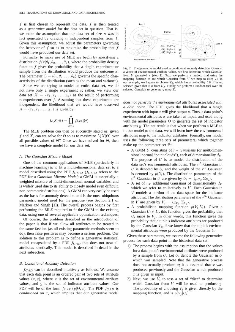
Fig. 2. The generative model used in conditional anomaly detection. Givenx,a vector of environmental attribute values, we first determine which Gaussianfrom U generatedx (step 1). Next, we perform a random trial using themapping function to see which Gaussian fromV we map to (step 2). Inour example, we happen to chooseV3, which has a probability 0.6 of beingselected given thatx is from U2. Finally, we perform a random trial over theselected Gaussian to generatey (step 3).

does not generate the environmental attributes associatedwitha data point. The PDF gives the likelihood that a singleexperiment with inputx will give outputy. Thus, a data point’senvironmental attributesx are taken as input, and used alongwith the model parametersΘ to generate the set of indicatorattributesy. The net result is that when we perform a MLE tofit our model to the data, we will learn how the environmentalattributes map to the indicator attributes. Formally, our modeluses the following three sets of parameters, which togethermake up the parameter setΘ:

• A GMM U consisting ofnU Gaussians (or multidimen-sional normal “point clouds”), each of dimensionalitydU .The purpose ofU is to model the distribution of thedata set’s environmental attributes. Theith Gaussian inU is denoted byUi and the weight of theith Gaussianis denoted byp(Ui). The distribution parameters of theith Gaussian inU are given byUi = 〈µUi

, ΣUi〉.

• A set of nV additional Gaussians of dimensionalitydV

which we refer to collectively asV . Each Gaussian inV models a portion of the data space for the indicatorattributes. The distribution parameters of thejth Gaussianin V are given byVj = 〈µVj

, ΣVj〉.

• A probabilistic mapping functionp(Vj |Ui). Given aGaussianUi ∈ U , this function gives the probability thatUi maps toVj . In other words, this function gives theprobability that a tuple’s indicator attributes are producedby the GaussianVj , if we know that the tuple’s environ-mental attributes were produced by the GaussianUi.

Given these parameters, we assume the following generativeprocess for each data point in the historical data set:

1) The process begins with the assumption that the valuesfor a data point’s environmental attributes were producedby a sample fromU . Let Ui denote the Gaussian inUwhich was sampled. Note that the generative processdoes not actually producex; it is assumed thatx wasproduced previously and the Gaussian which producedx is given as input.

2) Next, we useUi to toss a set of “dice” to determinewhich Gaussian fromV will be used to producey.The probability of choosingVj is given directly by themapping function, and isp(Vj |Ui).

IEEE TRANSACTIONS ON KNOWLEDGE AND DATA ENGINEERING 4

3) Finally, y is produced by taking a single sample fromthe Gaussian that was randomly selected in Step(2).The process of generating a value fory given a valuefor x is depicted above in Figure 2.

It is important to note that while our generative modelassumes that we know which Gaussian was used to generatex, in practice this information is not included in the dataset. We can only infer this by computing a probability thateach Gaussian inU was the one that producedx. As a result,fCAD (y|Θ, x) is defined as follows:

fCAD (y|Θ, x) =

nU∑

i=1

p (x ∈ Ui)

nV∑

j=1

fG (y|Vj) p (Vj |Ui)

Where:

• p(x ∈ Ui) is the probability thatx was produced by theith Gaussian inU , and is computed using Bayes’ rule:

p (x ∈ Ui) =fG (x|Ui) p (Ui)

PnUk=1

fG(x|Uk)p(Uk)

• fG(y|Vj) is the likelihood that thejth Gaussian inVwould producey, and is the standard Gaussian distribu-tion (see the Appendix).

• p(Vj |Ui) is the probability that theith Gaussian fromUmaps to thejth Gaussian fromV . This is given directlyas a parameter inΘ.

Given the functionfCAD(y|Θ, x), the problem of modeling adata set(X, Y ) can be succinctly stated as:

ChooseΘ so as to maximize

Λ =

n∑

k=1

log fCAD (yk|Θ, xk) over all possible values forΘ.

In this expression,Λ is referred to as thelog-likelihoodof theresulting model.

C. Detecting Conditional Anomalies

Like other parametric anomaly detection methods, themethodology for detecting future anomalies using the CADmodel is based on the observation that once an optimal valuefor Θ has been learned, the functionfCAD can be used to givea meaningful ordering over all data points past and future, fromthe most astonishing to the most typical. When a new pointis observed that has a small value forfCAD, this means thatit occurs in a portion of the data space with low density, andit should be flagged as an anomaly.

In order to determine the cutoff value forfCAD belowwhich a new point is determined to be anomalous, we allowthe user to first pick a fractionǫ from 0 to 1, and then wechoose thefCAD value such that exactly a fractionǫ of thedata points in the training set would have been flagged asanomalies. A high value ofǫ means that the method is lessselective, and hence it increases the chance that an anomalousevent will be flagged for further investigation. However, atthesame time this will tend to increase the rate of false positives.

Given ǫ and the size of the training data setn, in order tochoose a cutoff such that exactlyǫ% of the training pointswould be considered anomalous, we simply sort the training

data based upon theirfCAD values, from lowest to highest.Next, let c = ǫn. This is the index of the cutoff point in theexisting data set. Any future observation which is found to bemore unusual than thecth existing point will be termed ananomaly. To check if a point(xnew , ynew) is anomalous, wesimply check iffCAD(ynew|Θ, xnew) < fCAD(yc|Θ, xc). Ifyes, then the new observation is flagged as an anomaly.

III. L EARNING THE MODEL

Of course, defining a model likefCAD is not enough. It isalso necessary to define a process whereby it is possible toadjust the model parameters so that the model can be fittedto the existing data. In general, this type of maximization isintractable. This Section defines several learning algorithmsfor computing the model. The Section begins with a high-levelintroduction to theExpectation Maximization[13] frameworkthat serves as a basis for all three of the algorithms.

A. The Expectation Maximization Methodology

While EM is usually called an “algorithm”, in reality itis a generic technique for solving MLE problems. EM caneither be easy or nearly impossible to apply to a specific MLEproblem, but in general its application is non-trivial. We nowturn to a description of the EM methodology.

As mentioned previously, most interesting MLE problemsare computationally intractable. In practice, this intractabilityresults from one or more “hidden” variables that cannot beobserved in the data, and must be inferred simultaneously withthe MLE. In the conditional anomaly detection problem, thesehidden variables are the identities of the Gaussians that wereused to produce the environmental and indicator attributesof each data point in the historical data set. The fact thatthese variables are not observable makes the problem difficult;if these values were included in the data, then solving forΘ becomes a mostly straightforward maximization problemrelying on college-level calculus. The EM algorithm is usefulin precisely such cases. EM is an iterative method, whose basicoutline is as follows:

The Basic Expectation Maximization Algorithm1) While the model continues to improve:

a) LetΘ be the current “best guess” as to the optimalconfiguration of the model.

b) Let Θ be the next “best guess” as to the optimalconfiguration of the model.

c) E-Step: ComputeQ, the expected value ofΛ withrespect toΘ over all possible values of the hid-den parameters. The probability of observing eachpossible set of hidden parameter values (required tocompute the expectation ofΛ) is computed usingΘ.

d) M-Step: ChooseΘ so as to maximize the valuefor Q. Θ then becomes the new “best guess”.

EM sidesteps the problem of not knowing the values ofthe hidden parameters by instead considering the expectedvalue of the PDF with respect toall possible valuesof thehidden parameters. Since computing the expected value ofΛ

IEEE TRANSACTIONS ON KNOWLEDGE AND DATA ENGINEERING 5

with respect to the hidden parameters requires that we be ableto compute the probability of every possible configuration ofthe hidden parameters (and to do this we need to know theoptimal configurationΘ), at each iteration EM computes thisprobability with respect to the best guess so far forΘ. Thus,EM does not compute a globally optimal solution at eachiteration; rather, it computes a best guess as to the answer,which is guaranteed to improve at each iteration. EM has thedesirable property that while it does not always converge totheglobally optimal solution, it does always converge to a locallyoptimal solution, where no combination of slight “tweaks” ofthe various values inΘ can improve the value ofΛ.

B. The Direct-CAD Algorithm

The remainder of this Section outlines three different EMalgorithms for learning the CAD model over a data set. Thefirst of the three algorithms attempts to learn all of the param-eters simultaneously: the Gaussians that govern the generationof the environmental attributes, the Gaussians that governthe generation of the indicator attributes, and the mappingfunction between the two sets of Gaussians. This Sectiononly outlines the approach, and gives the equations that areused to implement the algorithm; the complete mathematicalderivation of the EM algorithm is quite involved and is leftto the Appendix II of the paper. As in any EM algorithm,the Direct-CAD algorithm relies on the two classic steps: theE-Stepand theM-Step.E-Step. To begin the process of deriving an appropriate EMalgorithm, we first need to define the hidden parameters inthe context of the conditional anomaly detection problem.In conditional anomaly detection, the hidden parameters arethe identities of the clusters fromU and V that were usedto produce each data point. To denote these parameters, wedefine:

• αk tells which cluster inU produced thekth value inX .α

(i)k denotes the assertion “thekth set of environmental

attributes was produced by theith cluster inU .”• βk tells which cluster inV produced thekth value in

Y . β(j)k denotes the assertion “thekth set of indicator

attributes was produced by thejth cluster inV .”

Given these variables, we can then derive theQ functionrequired by the E-Step of the EM algorithm. LetQ(Θ, Θ)denote the expected value ofΛ over all possibleα, β given thecurrent parameter valuesΘ. Then, as derived in the AppendixII:

Q(Θ, Θ)

=E[

n∑

k=1

log fCAD(xk,yk, αk, βk|xk, Θ)|X, Y, Θ]

=n

∑

k=1

nU∑

i=1

nV∑

j=1

log fG(yk|Vj , Θ) + log p(Vj |Ui, Θ)

+ log fG(xk|Ui, Θ) + log p(Ui)− log f(xk|Θ)

× bkij

Where:

bkij =fG(xk|Ui)p(Ui)fG(yk|Vj)p(Vj |Ui, Θ)

nU∑

t=1

nV∑

h=1

{fG(xk|Ut)p(Ut)fG(yk|Vh)p(Vh|Ut, Θ)}

M-Step. In the M-Step, we now use standard calculus tomaximize the value ofQ over all Θ. This results in a seriesof equations that can be used to compute the new parametervalues that will be used during the next iteration. The detailsof the derivation of each of the equations are reasonablyinvolved and are given in the Appendix. However, theuseof the equations is relatively straightforward, and requiresonly that we perform standard arithmetic and linear algebraoperations over the previous model parameters and the dataset. The formulas for the components ofΘ are as follows:

• p(Ui) =

n∑

k=1

nV∑

j=1

bkij/

n∑

k=1

nU∑

h=1

nV∑

j=1

bkhj

• µUi=

n∑

k=1

nV∑

j=1

bkijxk/n

∑

k=1

nV∑

j=1

bkij

• ΣUi=

n∑

k=1

nV∑

j=1

bkij(xk − µUi)(xk − µUi

)T /

n∑

k=1

nV∑

j=1

bkij

• µVj=

n∑

k=1

nU∑

i=1

bkijyk/

n∑

k=1

nU∑

i=1

bkij

• ΣVj=

n∑

k=1

nU∑

i=1

bkij(yk − µVj)(yk − µVj

)T /

n∑

k=1

nU∑

i=1

bkij

• p(Vj |Ui) =

n∑

k=1

bkij/

n∑

k=1

nV∑

h=1

bkih

Given the update rules described above, our EM algorithm forlearning the conditional anomaly detection model is then asfollows:

The Direct-CAD Algorithm1) Choose an initial set of values for〈µVj

, ΣVj〉, 〈µUi

,ΣUi

〉, p(Vj |Ui), p(Ui), for all i, j.2) While the model continues to improve (measured by the

improvement ofΛ):

a) Computebkij for all k, i, andj as described underE-Step above;

b) Compute〈µVj, ΣVj

〉, 〈µUi, ΣUi

〉, p(Vj |Ui), p(Ui)for all i, j as described underM-Step above;

c) Set 〈µVj, ΣVj

〉 := 〈µVj, ΣVj

〉, 〈µUi, ΣUi

〉 :=〈µUi

, ΣUi〉, p(Vj |Ui) := p(Vj |Ui), p(Ui) := p(Ui)

for all i, j.The time and space requirements of this algorithm can

be derived as follows. To computebkij in the E-Step,we first computefG(xk|Ui) and fG(yk|Vj), which takesO(nnUd2

U ) time and O(nnV d2V ) time, respectively. Then it

takes O(nnUnV ) time to compute all thebkij values. In theM-Step, we update the value for each component ofΘ. Ittakes O(nnUnV d2

U ) time to updateΣUi, and O(nnUnV d2

V )time to updateΣVj

. To update the rest of the components, thetime complexity is O(nnUnV (dU + dV + nV )). Adding themtogether, the time complexity for one iteration (E-Step andM-Step) is O(nnUnV (d2

U + d2V )). The total time complexity

of the conditional anomaly detection algorithm depends on

IEEE TRANSACTIONS ON KNOWLEDGE AND DATA ENGINEERING 6

the convergence speed, i.e., the number of iterations, whichdepends on the data set itself.

Accordingly, in the E-Step, storing the results forfG(xk|Ui), fG(yk|Vj) and bkij requires O(nnUnV ) space.Storing the updated components ofΘ requires O(nUd2

U +nV d2

V ) space.

C. The GMM-CAD-Full Algorithm

Unfortunately, the algorithm described in the previous Sub-section has a major potential drawback. The EM approachis known to be somewhat sensitive to converging to locallyoptimal solutions that are far from the globally optimal so-lution, particularly when it is used in conjunction with verycomplex optimization problems. While standard methods suchas multiple runs with randomized seeds may help [15], theproblem remains that the CAD problem is certainly complexas MLE problems go, since the task is to simultaneouslylearn two sets of Gaussians as well as a mapping function,and the problem is complicated even more by the fact thatthe functionfCAD is only conditionally dependent upon theset of Gaussians corresponding to the distribution of theenvironmental attributes.

As a result, the second learning algorithm that we considerin this paper makes use of a two-step process. We begin byassuming that the number of Gaussians inU andV is identical;that is, nU = nV . Given this, a set of Gaussians is learnedin the combinedenvironmental and indicator attribute space.These Gaussians are then projected onto the environmentalattributes and indicator attributes to obtainU and V . Then,only after U and V have been fixed, a simplified version ofthe Direct-CAD algorithm is used to compute only the valuesp(Vi|Uj) that make up the mapping function. The benefit ofthis approach is that by breaking the problem into two, mucheasier optimization tasks, each solved by much simpler EMalgorithms, we may be less vulnerable to the problem oflocal optima. The drawback of this approach is that we areno longer trying to maximizefCAD directly; we have madethe simplifying assumption that it suffices tofirst learn theGaussians, andthen learn the mapping function.

The GMM-CAD-Full Algorithm1) Learn a set ofnU (dU +dV )-dimensional Gaussians over

the data set{(x1, y1), (x2, y2), ..., (xn, yn)}. Call thissetZ.

2) Let µZirefer to the centroid of theith Gaussian inZ,

and let ΣZirefer to the covariance matrix of theith

Gaussian inZ. We then determineU as follows:For i = 1 to nU do:

p(Ui) := p(Zi)For j = 1 to dU do:

µUi[j] := µZi

[j]For k = 1 to dU do:

ΣUi[j][k] := ΣZi

[j][k]3) Next, determineV as follows:

For i = 1 to nV do:For j = 1 to dV do:

µVi[j] := µZi

[j + dU ]For k = 1 to dV do:

ΣVi[j][k] := ΣZi

[j+dU ][k+dU ]

4) Run a second EM algorithm to learn the mapping func-tion. While the model continues to improve (measuredby the improvement ofΛ):

a) Computebkij for all k, i, andj as in the previousSubsection.

b) Computep(Vj |Ui) as described in the previousSubsection.

c) Setp(Vj |Ui) := p(Vj |Ui).

The time required for the GMM-CAD-Full algorithm con-sists of two parts: the time to learn the Gaussians, which isO(nnU (dU +dV )2), and the time to learn the mapping functionby simplified Direct-CAD algorithm, which is O(nn3

U ). Thememory required for GMM-CAD-Full algorithm is O(nnU +nU (dU + dV )2).

D. The GMM-CAD-Split Algorithm

There is a third obvious way to learn the required model,that is closely related to the previous one. Since the previousalgorithm breaks up the optimization problem into two smallerproblems, there is no longer any reason to think that theGMMs for U andV should be learned simultaneously. Learn-ing them simultaneously might actually be overly restrictive,since learning them simultaneously will try to learnU andVso that every Gaussian inU is “mated” to a Gaussian inVthrough a covariance structure. The CAD model has no suchrequirement, since the Gaussians ofU andV are related onlythrough the mapping function. In fact, the algorithm from theprevious Subsection throws out all of this additional covarianceinformation sinceΣZi

[j][k] is never used for(j ≤ dU , k >dU ) or (j > dU , k ≤ dU ).

As a result, the third algorithm we consider learnsU andVdirectly as two separate GMMs, and then learns the mappingfunction between them. The algorithm is outlined below.

The GMM-CAD-Split Algorithm1) LearnU and V by performing two separate EM opti-

mizations.2) Run Step (4) from the GMM-CAD-Full Algorithm to

learn the mapping function.

In GMM-CAD-Split algorithm, learning Gaussians in Uand V needs O(nnU (d2

U + d2V )) time. Learning the mapping

function needs O(nn3U ) time. The memory requirement for the

algorithm is O(nnU + nU (d2U + d2

V )).

E. Choosing the Complexity of the Model

Whatever learning algorithm is used, it is necessary tochoose as an input parameter the number of clusters orGaussians in the model. In general, it is difficult to choosethe optimal value of the number of Gaussians in a GMM,and this is a research problem on its own [16]. However, ourproblem is a bit easier because we are not actually trying tocluster the data for the sake of producing a clustering; rather,we are simply trying to build an accurate model for the data.In our experiments, we generally found that a larger number ofclusters in the CAD model results in more accuracy. It is truethat a very large number of clusters could cause over-fitting,but in the CAD model, the computational cost associated with

IEEE TRANSACTIONS ON KNOWLEDGE AND DATA ENGINEERING 7

any model large enough to cause over-fitting makes it virtuallyimpossible to over-fit a data set of reasonable size. Thus,our recommendation is to choose the largest model that canbe comfortably computed. In our implementation, we use 40clusters for bothU andV .

IV. B ENCHMARKING

In this Section, we describe a set of experiments aimed attesting the effectiveness of the CAD model. Our experimentsare aimed at answering the following three questions:

1) Which of the three learning algorithms should be usedto fit the CAD model to a data set?

2) Can use of the CAD model reduce the incidence offalse positives due to unusual values for environmentalattributes compared to obvious alternatives for use in ananomaly detection system?

3) If so, does the reduced incidence of false positives comeat the expense of a lower detection level for actualanomalies?

A. Experimental Setup

Unfortunately, as with any unsupervised learning task, itcan be very difficult to answer questions regarding the qualityof the resulting models. Though the quality of the models ishard to measure, we assert that with a careful experimentaldesign, itis possible to give a strong indication of the answerto our questions. Our experiments are based on the followingkey assumptions:

• Most of the points in a given data set are not anomalous,and so a random sample of a data set’s points shouldcontain relatively few anomalies.

• If we take a random sample of a data set’s points andperturb them by swapping various attribute values amongthem, then the resulting set of data points should contain amuch higher fraction of anomalies than a simple randomsample from the data set.

Given these assumptions, our experimental design is as fol-lows. For each data set, the following protocol was repeatedten times:

1) For a given data set, we begin by randomly designating80% of the data points astraining data, and20% of thedata points astest data(this latter set will be referredto astestData).

2) Next, 20% anomalies or outliers in the settestDataare identified using a standard, parametric test based onGaussian mixture modeling – the data are modeled usinga GMM and new data points are ranked as potentialoutliers based on the probability density at the point inquestion. This basic method is embodied in more thana dozen papers cited in Markou and Singh’s survey [1].However, a key aspect of this protocol is thatoutliers arechosen based only on the values of their environmentalattributes(indicator attributes are ignored). We call thissetoutliers.

3) The set testData is then itself randomly parti-tioned into two identically-sized subsets:perturbed and

nonPerturbed, subject to the constraint thatoutliers ⊂nonPerturbed.

4) Next, the members of the setperturbed are perturbedby swapping indicator attribute values among them.

5) Finally, we use the anomaly detection software tocheck for anomalies amongtestData = perturbed ∪nonPerturbed.

Note that after this protocol has been executed, members ofthe setperturbed are no longer samples from the original datadistribution, and members of the setnonPerturbed are stillsamples from the original data distribution. Thus, it shouldbe relatively straightforward to use the resulting data sets todifferentiate between a robust anomaly detection framework,and one that is susceptible to high rates of false positives.Specifically, given this experimental setup, we expect thatauseful anomaly detection mechanism would:

• Indicate that a relatively large fraction of the setperturbed are anomalies; and

• Indicate that a much smaller fraction of the setnonPerturbed are anomalies; and

• Indicate that a similarly small fraction of the setoutliersare anomalies.

This last point bears some further discussion. Since theserecords are also samples from the original data distribution,the only difference betweenoutliers and (nonPerturbed −outliers) is that the records inoutliers have exceptionalvalues for their environmental attributes. Given the definitionof an environmental attribute, these should not be consideredanomalous by a useful anomaly detection methodology. Infact, the ideal test result would show that the percentageof anomalies amongoutliers is identical to the percentageof anomalies amongnonPerturbed. A high percentage ofanomalies among the setoutliers would be indicative of atendency towards false alarms in the case of anomalous (butuninteresting) values for environmental attributes.

B. Creating the SetPerturbed

The above testing protocol requires that we be able tocreate a set of pointsperturbed with an expectedly highpercentage of anomalies. An easy option would have beento generate perturbed data by adding noise. However, this canproduce meaningless (or less meaningful) values of attributes.We wanted to ensure that the perturbed data is structurallysimilar to the original distribution and domain values so thatit is not trivial to recognize members of this set because theyhave similar characteristics compared to the training data(thatis, the environmental attributes are realistic and the indicatorattributes are realistic, but the relationship between them maynot be). We achieve this through a natural perturbation scheme:

Let D be the set of data records that has been chosen fromtestData for perturbation. Consider a recordz = (x, y) fromD that we wish to perturb. Recall from Section 2.2 thatx isa vector of environmental attribute values andy is a vector ofindicator attribute values. To perturbz, we randomly choosekdata points fromD; in our tests, we usek = min(50, |D|/4).Let z′ = (x′, y′) be the sampled record such that the Euclideandistance betweeny andy′ is maximized over allk of our sampleddata points. To perturbz, we simply create a new data point(x, y′), and add this point toperturbed.

IEEE TRANSACTIONS ON KNOWLEDGE AND DATA ENGINEERING 8

This process is iteratively applied to all points in theset D to perturbed. Note that every set of environmentalattribute values present inD is also present inperturbed afterperturbation. Furthermore, every set of indicator attributespresent inperturbed after perturbation is also present inD. What has been changed is only therelationshipbetweenthe environmental and indicator attributes in the records ofperturbed.

We note that swapping the indicator values may not alwaysproduce the desired anomalies (it is possible that some of theswaps may result in perfectly typical data). However, swappingthe valuesshould result in a new data set that has a largerfraction of anomalies as compared to sampling the data setfrom its original distribution, simply because the new datahasnot been sampled from the original distribution. Since someof the perturbed points may not be abnormal, even a perfectmethod should deem a small fraction of theperturbedset to benormal. Effectively, this will create a non-zero false negativerate, even for a “perfect” classifier. Despite this, the experimentis still a valid one because each of the methods that we testmust face this same handicap.

C. Data Sets Tested

We performed the tests outlined above over the followingthirteen data sets1. For each data set, the annotation(i × j)indicates that the data set hadi environmental andj indicatorattributes, which were chosen after a careful evaluation ofthedata semantics. A brief description of the environmental andindicator attributes for each data set is also given. The thirteendata sets used in testing are:

1) Syntheticdata set(50 × 50). Synthetic data set created using theCAD model. 10,000 data points were sampled from the generativemodelf . f has 10 Gaussians inU andV respectively. The centroidsof the Gaussians are random vectors whose entries are chosenon theinterval (0.0, 1.0). The diagonal of the covariance matrix is set to1/4of the average distance between the centroids in each dimension. Theweight of the Gaussians is evenly assigned and the mapping functionP (Vj |Ui) for a certain value ofi is a permutation of geometricdistribution.

2) Algae data set(11 × 6). The data is from UCI KDD Archive. Weremoved the data records with missing values. The environmentalattributes consist of the season, the river size, the fluid velocity,and some chemical concentrations. The indicator attributes are thedistributions of different kinds of algae in surface water.

3) Streamflowdata set(205 × 100). The data set depicts the river flowlevels (indicator) and precipitation and temperature (environmental) forCalifornia. We create this data set by concatenating the environmentaland indicator data sets. The environmental data set is obtained fromNational Climate Data Center (NCDC). The indicator data setisobtained from U.S. Geological Survey (USGS).

4) ElNino data set(4 × 5). The data is from UCI KDD Archive. Itcontains oceanographic and surface meteorological readings takenfrom a series of buoys positioned throughout the equatorialPacific.The environmental attributes are the spatio-temporal information. Theindicator attributes are the wind direction, relative humidity andtemperature at various locations in the Pacific Ocean.

5) Physicsdata set(669× 70). The data is from KDD Cup 2003. For alarge set of physics papers, we pick out frequency information for keywords (environmental) and a list of most referred articles (indicator).One data record, which represents one physics paper, has 0/1-valuedattributes, corresponding to the appearance/absence of the key word(or referred-to article) respectively.

1we have conducted an experiment on a pre-labeled data set as suggested.Refer to Appendix I for the results

6) Bodyfatdata set(13×2). The data is from CMU statlib. It depicts bodyfat percentages (indicator) and physical characteristics(environmental)for a group of people.

7) Housesdata set(8×1). The data is from CMU statlib. It depicts houseprice (indicator) in California and related environmentalcharacteristics(environmental) such as median income, housing median age,totalrooms, etc.

8) Bostondata set(15× 1). The data is from CMU statlib. We removedsome attributes that are not related to environmental-indicator rela-tionship. The data depicts the house value of owner-occupied homes(indicator) and economic data (environmental) for Boston.

9) FCAT-mathdata set(14 × 12). The data is from National Centerfor Education Statistics (NCES) and Florida Information ResourceNetwork (FIRN). We removed the data records with missing values.It depicts Mathematics achievement test results (indicator) of grade 3of year 2002 and regular elementary schools’ characteristics (environ-mental) for Florida.

10) FCAT-readingdata set(14 × 11). The data is also from NCES andFIRN. We processed the data similarly as with the FCAT-math data set.It depicts the reading achievement test scores (indicator)and regularelementary schools’ characteristics (environmental) forFlorida.

11) FLFarms data set(114 × 52). The data set depicts the Florida statefarms’ market value in various aspects (indicator) and the farms’operational and products statistics (environmental).

12) CAFarmsdata set(115 × 51). The data set depicts the Californiastate farms’ market value in various aspects (indicator) and the farms’operational and products statistics (environmental).

13) CAPeaksdata set(2 × 1). The data set depicts the California peaks’height (indicator) and longitude and altitude position (environmental).

D. Experimental Results

We performed the tests described above over six alternativesfor anomaly detection:

1) Simple Gaussian mixture modeling (as described at thebeginning of this Section). In this method, for each dataset a GMM model is learned directly over the trainingdata. Next, the settestData is processed, and anomaliesare determined based on the value of the functionfGMM

for each record intestData; those with the smallestfGMM values are considered anomalous.

2) kth-NN (kth nearest neighbor) outlier detection [9] (withk = 5). kth-NN outlier detection is one of the mostwell-known methods for outlier detection. In order tomake it applicable to the training/testing framework weconsider, the method must be modified slightly, sinceeach test data point must be scored in order to describethe extent to which it deviates from the training set.Given a training data set, in order to use the5th methodin order to determine the degree to which a test point isanomalous, we simply use the distance from the pointto its 5th in the training set. A larger distance indicatesa more anomalous point.

3) Local outlier factor (LOF) anomaly detection [8]. LOFmust be modified in a matter similar tokth-NN outlierdetection: the LOF of each test point is computed withrespect to the training data set in order to score the point.

4) Conditional anomaly detection, with the model con-structed using the Direct-CAD Algorithm.

5) Conditional anomaly detection, with the model con-structed using the GMM-CAD-Full Algorithm.

6) Conditional anomaly detection, with the model con-structed using the GMM-CAD-Split Algorithm.

For each experiment over each data set with the GMM/CADmethods, a data record was considered an anomaly if the

IEEE TRANSACTIONS ON KNOWLEDGE AND DATA ENGINEERING 9

probability density at the data point was less than the medianprobability density at all of the test data points. For5th-NN/LOF, the record was considered an anomaly if its distancewas greater than the median distance over all test data points.The median was used because exactly one-half of the points inthe settestData were perturbed. Thus, if the method was ableto order the data points so that all anomalies were before allnon-anomalies, choosing the median density should result ina recall2 rate of100% and a false positive rate of0% (a falsepositive rate of0% is equivalent to a precision3 of 100%). Alsonote that since exactly one-half of the points are perturbedandeach method is asked to guess which half are perturbed, it isalways the case that the recall is exactly equal to the precisionwhen identifying either anomalous or non-anomalous recordsin this experiment.

The results are summarized in the two tables below. Thefirst table summarizes and compares the quality of the re-call/precision obtained when identifying perturbed points intestData. Each cell indicates which of the two methodscompared in the cell was found to be the “winner” in terms ofhaving superior recall/precision over the13 sets. To computethe “winner”, we do the following. For each of the13 sets andeach pair of detection methods, the recall/precision of thetwomethods is averaged over the10 different training/testing parti-tionings of the data set. Letmethod1 andmethod2 be the twoanomaly detection methods considered in a cell.method1 issaid to “win” the test if it has a higher average recall/precisionin 7 or more of the13 data sets. Likewise,method2 is declaredthe winner if it has a higher recall/precision in7 or more ofthe data sets. In addition, we also give the number of the13data sets for which the winning method performed better, andwe give ap-value that indicates the significance of the results.

Finally, the second column in the table gives the averagerecall/precision over all experiments for each method. Thisis the average percentage of perturbed points that have prob-ability density less than the median (for GMM and CAD)or have a score/distance greater than the median (LOF and5th-NN) Though these numbers are informative, we cautionthat the number of head-to-head wins is probably a betterway to compare two methods. The reason for this is that therecall/precision can vary significantly from data set to data set,and thus the average may tend to over-weight those data setsthat are particularly difficult.

This p-value addresses the following question. Imaginethat the whole experiment was repeated by choosing a new,arbitrary set of13 datasets at random, and performing10different training/testing partitionings of each data set. Thep-value gives the probability that we would obtain a differentwinner than was observed in our experiments due to choosingdifferent data sets and partitionings. A lowp-value meansthat it is unlikely that the observed winner was due mostlyto chance, and so the results are significant. A highp-valuemeans that if the experiment was repeated again with a newset of data sets, the result may be different. Thep-value was

2Recall in this context is the fraction of perturbed points that are flaggedas anomalies.

3Precision in this context is the fraction of anomalies that are actuallyperturbed points.

computed using a bootstrap re-sampling procedure [17].The second table is similar to the first, but rather than

comparing the recall/precision with which the methods canidentify the perturbed points, it summarizes the recall/precisionin identifying as non-anomalous points in the setoutliers.Recall that theoutliers set are points with exceptional valuesfor their environmental attributes, but which are non-perturbedand so they are actually obtained from the training distribution.Thus, this table gives an indication of how successful thevarious methods are in ignoring anomalous environmentalattributes when the points were in fact sampled from thebaseline (or training) distribution. Just as in the first table,each cell gives the winner, the number of trials won, and theassociatedp-value of the experiment. The second column givesthe average precision/recall. This is the percentage of non-perturbed points with exceptional environmental attributes thatwere considered to be non-anomalous.

E. Discussion

Our experiments were designed to answer the followingquestion: If a human expert wishes to identify a set ofenvironmental attributes that should not be directly indicativeof an anomaly, can any of the methods successfully ignoreexceptional values for those attributes while at the same timetaking them into account when performing anomaly detection?

The first part of the question is addressed by the resultsgiven in Table II. This Table shows that if the goal is to ignoreanomalous values among the environmental attributes, thenthe CAD-GMM-Full algorithm is likely the best choice. Thismethod declared the lowest percentage of data points withexceptional environmental attribute values to be anomalous.In every head-to-head comparison, it did a better job for atleast 77% of the data sets (or10 out of 13).

The second part of the question is addressed by the resultsgiven in Table I. This table shows that if the goal is to notonly ignore exceptional environmental attributes, but also totake the normal correlation between environmental attributesand the indicator attributes into account, then the CAD-GMM-Full algorithm is again the best choice. Table I shows thatcompared to all of the other options, this method was bestable to spot cases where the indicator attributes were not in-keeping with the environmental attributes because they hadbeen swapped.

Finally, it is also important to point out that no method wasuniformly preferable to any other method for each and everydata set tested. It is probably unrealistic to expect that anymethodwouldbe uniformly preferable. For example, we foundthe the CAD-based methods generally did better comparedto the two distance-based methods (and the GMM method)on higher-dimensional data. The results were most strikingfor the thousand-dimensional physics paper data set, wherethe precision/recall for LOF and5th-NN when identifyingperturbed data was worse than a randomized labeling wouldhave done (less than50%). In this case, each of the CADmethods had greater than90% precision/recall. For lower-dimensional data, the results were more mixed. Out of all ofthe head-to-head comparisons reported in Tables I and II, there

IEEE TRANSACTIONS ON KNOWLEDGE AND DATA ENGINEERING 10

TABLE I

HEAD-TO-HEAD WINNER WHEN COMPARING RECALL/PRECISION FOR IDENTIFYING PERTURBED DATA AS ANOMALOUS(EACH CELL HAS WINNER, WINS

OUT OF13 DATA SETS, BOOTSTRAPPEDp-VALUE )

Avg rcl/prc CAD-Full CAD-Split Direct CAD 5th-NN LOF

GMM .720 Full, 11, 0.01 Split, 8, 0.25 CAD, 8, 0.35 GMM, 8, 0.25 GMM, 8, 0.16CAD-Full .793 – Full, 10, 0.04 Full, 10, 0.03 Full, 10, 0.01 Full, 10, 0.01CAD-Split .737 – – Split, 7, 0.47 Split, 7, 0.41 Split, 8, 0.23

Direct CAD .730 – – – CAD, 8, 0.28 CAD, 9, 0.13

5th-NN .721 – – – – 5th-NN, 7, 0.41LOF .721 – – – – –

TABLE II

HEAD-TO-HEAD WINNER WHEN COMPARING RECALL/PRECISION FOR IDENTIFYING NON-PERTURBED OUTLIER DATA AS NON-ANOMALOUS (EACH CELL

HAS WINNER, WINS OUT OF13 DATA SETS, BOOTSTRAPPEDp-VALUE )

Avg rcl/prc CAD-Full CAD-Split Direct CAD 5th-NN LOF

GMM .500 Full, 12, 0.00 Split, 10, 0.06 CAD, 9, 0.12 GMM, 9, 0.23 GMM, 7, 0.34CAD-Full .749 – Full, 11, 0.01 Full, 10, 0.01 Full, 13, 0.00 Full, 10, 0.01CAD-Split .687 – – CAD, 7, 0.49 Split, 10, 0.01 Split, 9, 0.09

Direct CAD .681 – – – CAD, 11, 0.00 CAD, 9, 0.125th-NN .500 – – – – LOF, 7, 0.37

LOF .549 – – – – –

is only one case where any method won13 out of 13 times(CAD-GMM-Full vs. LOF in terms of the ability to ignoreanomalous environmental attributes). Thus, our results donotimply that any method will do better than any other methodon an arbitrary data set. What the resultsdo imply is that ifthe goal is to choose the method that ismost likelyto do betteron an arbitrary data set, then the CAD-GMM-Full algorithmis the best choice.

V. RELATED WORK

Anomaly and outlier detection have been widely studied,and the breadth and depth of the existing research in the areaprecludes a detailed summary here. An excellent survey ofso-called “statistical” approaches to anomaly detection canbe found in Markou and Singh’s 2003 survey [1]. In thiscontext, “statistical” refers to methods which try to identifythe underlying generative distribution for the data, and thenidentify points that do not seem to belong to that distribution.Markou and Singh give references to around a dozen papers,that, like the CAD methodology, rely in some capacity onGaussian Mixture Modeling to represent the underlying datadistribution. However, unlike the CAD methodology, nearlyall of those papers implicitly assume that all attributes shouldbe treated equally during the detection process.

The specific application area of intrusion detection is thetopic of literally hundreds of papers that are related toanomaly detection. Unfortunately, space precludes a detailedsurvey of methods for intrusion detection here. One keydifference between much of this work and our own proposalis the specificity: most methods for intrusion detection arespecifically tailored to that problem, and are not targetedtowards the generic problem of anomaly detection, as the CADmethodology is. An interesting 2003 study by Lazarevic et al.[18] considers the application of generic anomaly detectionmethods to the specific problem of intrusion detection. The

authors test several methods and conclude that LOF [8] (testedin this paper) does a particularly good job in that domain.

While most general-purpose methods assume that all at-tributes are equally important, there are some exceptions tothis. Aggarwal and Yu [19] describe a method for identifyingoutliers in subspaces of the entire data space. Their methodidentifies combinations of attributes where outliers are particu-larly obvious, the idea being that a large number of dimensionscan obscure outliers by introducing noise (the so-called “curseof dimensionality” [20]). By considering subspaces, this effectcan be mitigated. However, Aggarwal and Yu make noa prioridistinctions among the types of attribute values using domainknowledge, as is done in the CAD methodology.

One body of work on anomaly detection originating instatistics that does make ana priori distinction among differentattribute types in much the same way as the CAD methodologyis so-calledspatial scan statistics[21][22][23]. In this work,data are aggregated based upon their spatial location, andthen the spatial distribution is scanned for sparse or denseareas. Spatial attributes are treated in a fashion analogous toenvironmental attributes in the CAD methodology, in the sensethat they are not taken as direct evidence of an anomaly; rather,the expected sparsity or density is conditioned on the spatialattributes. However, such statistics are limited in that theycannot easily be extended to multiple indicator attributes(theindicator attribute is assumed to be a single count), nor aretheymeant to handle the sparsity and computational complexitythat accompany large numbers of environmental attributes.

The existing work that is probably closest in spirit to ourown is likely the paper on anomaly detection for findingdisease outbreaks by Wong, Moore, Cooper, and Wagner[24]. Their work makes use of a Bayes Net as a baseline todescribe possible environmental structures for a large numberof input variables. However, because their method relies ona Bayes Net, there are certain limitations inherent to thisapproach. The most significant limitation of relying on a

IEEE TRANSACTIONS ON KNOWLEDGE AND DATA ENGINEERING 11

Bayes Net is that continuous phenomena are hard to describein this framework. Among other issues, this makes it verydifficult to describe the temporal patterns such as time lagsand periodicity. Furthermore, a Bayes Net implicitly assumesthat even complex phenomena can be described in termsof interaction between a few environmental attributes, andthat there are no hidden variables unseen in the data, whichis not true in real situations where many hidden attributesand missing values are commonplace. A Bayes Net cannotlearn two different explanations for observed phenomena andlearn to recognize both, for it cannot recognize unobservedvariables. Such hidden variables are precisely the type ofinformation captured by the use of multiple Gaussian clustersin our model; each Gaussian corresponds to a different hiddenstate.

Finally, we mention that traditional prediction models, suchas linear or nonlinear models of regression [25][26] can also bepotentially used for deriving the cause-effect interrelationshipsthat the CAD method uses. For example, for a given set ofenvironmental attribute values, a trained regression model willpredict the indicator attribute value, and by comparing it withthe actual indicator attribute value, we can determine if thetest point is anomalous or not. However, there are importantlimitations on such regression methods as compared to theCAD model. First, in regression there is typically one responsevariable (indicator variable) and multiple predictor variables(environmental variables), while the CAD method allows anarbitrary number of indicator attributes. Second, it is unclearhow a regression-based methodology could be used to rankthe interest of data points based on their indicator attributes.Distance from the predicted value could be used, but thisseems somewhat arbitrary, since the natural variation maychange depending on indicator attribute values.

VI. CONCLUSIONS ANDFUTURE WORK

In this paper we have described a new approach to anomalydetection. We take a rigorous, statistical approach where thevarious data attributes are partitioned intoenvironmentalandindicator attributes, and a new observation is consideredanomalous if its indicator attributes cannot be explained inthe context of the environmental attributes. There are manyavenues for future work. For example, we have consideredonly one way to take into account a very simple type ofdomain knowledge to boost the accuracy of anomaly detection.How might more complex domain knowledge boost accuracyeven more? For another example, an important issue that wehave not addressed is scalability during the construction of themodel. While the model can always quickly and efficiently beused to check for new anomalies, training the model on amulti-gigabyte database may be slow without a modificationof our algorithms. One way to address this may be to use avariation of the techniques of Bradley et al. [27] for scalingstandard, Gaussian EM to clustering of very large databases.

APPENDIX IEXPERIMENT ONKDD CUP 1999DATASET

One of the anonymous referees for the paper suggestedthat we apply our algorithms to the KDD Cup 1999 data set.

GMM CAD−Full CAD−Split Direct CAD 5th−NN LOF0.75

0.8

0.85

0.9

0.95

1

prec

isio

n

Fig. 3. Precision rate on KDD Cup 1999 data set by 10-fold cross-validation.The minimum and maximum precision rates over 10 runs are depicted ascircles and the overall precision is depicted as a star sign

Unlike the thirteen data sets described in the paper, this dataset is labeled, and so we know if a particular test record isactually anomalous. After partitioning into causal and resultattributes, we used a 10-fold cross-validation test to comparethe precision of the different detection methods on this dataset; error bars showing the low and high accuracy of eachmethod as well as the mean are provided in Figure 3. Theresults show that this particular task is rather easy, and soit isdifficult to draw any additional conclusions from the results.All of the methods except for LOF perform very well, withalmost perfect overlap among the error bars.

APPENDIX IIEM DERIVATIONS

A. MLE Goal.

The goal is to maximize the objective function:

Λ = log

n∏

k=1

fCAD(yk|xk)

=

n∑

k=1

log

nU∑

i=1

p(xk ∈ Ui)

nV∑

j=1

fG(yk|Vj)p(Vj |Ui)

(1)

where:

fCAD(yk|xk) =

nU∑

i=1

p(xk ∈ Ui)

nV∑

j=1

fG(yk|Vj)p(Vj |Ui) (2)

B. Expectation Step.

The expectation of the objective function is:

Q(Θ, Θ)

=E[Λ(X, Y, α, β|X, Θ)|X, Y, Θ]

=E[n

∑

k=1

log fCAD(xk,yk, αk, βk|xk, Θ)|X, Y, Θ]

=

n∑

k=1

∑

αk

∑

βk

{log fCAD(yk, αk, βk|xk, Θ)f(αk, βk|X, Y, Θ)}

=

n∑

k=1

nU∑

i=1

nV∑

j=1

{log fCAD(yk, α(i)k , β

(j)k |xk, Θ)

× f(α(i)k , β

(j)k |xk, yk, Θ)} (3)

IEEE TRANSACTIONS ON KNOWLEDGE AND DATA ENGINEERING 12

Now we derive the two sub-expressions in(3):

f(α(i)k , β

(j)k |xk, yk, Θ)

=f(xk, α

(i)k , yk, β

(j)k |Θ)

f(xk, yk|Θ)

=f(xk, α

(i)k |Θ)f(yk, β

(j)k |xk, α

(i)k , Θ)

f(xk|Θ)f(yk|xk, Θ)

=f(xk, α

(i)k |Θ)f(yk, β

(j)k |xk, α

(i)k , Θ)

f(xk|Θ)

nU∑

t=1

{

p(xk ∈ Ut, Θ)

nV∑

h=1

[fG(yk|Vh)p(Vh|Ut, Θ)]

}

(4)

Since:

f(xk, α(i)k |Θ) = f(xk, Ui|Θ) = fG(xk|Ui)p(Ui) (5)

Through(2), we can get:

f(yk, β(j)k |xk, α

(i)k , Θ) = fG(yk|Vj)p(Vj |Ui, Θ) (6)

nU∑

i=1

p(xk ∈ Ui) = 1, p(xk ∈ Ut) is the membership ofxk in

clusterUt, so:

p(xk ∈ Ut, Θ) =fG(xk|Ut)p(Ut)

nU∑

i=1

fG(xk|Ui)p(Ui)

=fG(xk|Ut)p(Ut)

f(xk|Θ)

(7)

Inserting (5), (6) and (7) into (4), we get:

f(α(i)k , β

(j)k |xk, yk, Θ)

=fG(xk|Ui)p(Ui)fG(yk|Vj)p(Vj |Ui, Θ)

nU∑

t=1

nV∑

h=1

{fG(xk|Ut)p(Ut)fG(yk|Vh)p(Vh|Ut, Θ)}

(8)

For simplicity, we introducebkij :

bkij = f(α(i)k , β

(j)k |xk, yk, Θ) (9)

With the new denotationbkij , the Q function in (3) be-comes:

Q(Θ, Θ)

=

n∑

k=1

nU∑

i=1

nV∑

j=1

{

log fCAD(yk, α(i)k , β

(j)k |xk, Θ) × bkij

}

(10)

where:

bkij =fG(xk|Ui)p(Ui)fG(yk|Vj)p(Vj |Ui, Θ)

nU∑

t=1

nV∑

h=1

{fG(xk|Ut)p(Ut)fG(yk|Vh)p(Vh|Ut, Θ)}

(11)

The remaining sub-expression inQ function is:

fCAD(yk, α(i)k , β

(j)k |xk, Θ)

=f(yk, β(j)k |xk, α

(i)k , Θ) × f(α

(i)k |xk, Θ)

=fG(yk|Vj) × p(Vj |Ui, Θ) ×fG(xk|Ui)p(Ui)

f(xk|Θ)(12)

Inserting (12) into (10), theQ function becomes:

Q(Θ, Θ)

=n

∑

k=1

nU∑

i=1

nV∑

j=1

log fG(yk|Vj) + log p(Vj |Ui, Θ)

+ log fG(xk|Ui) + log p(Ui)− log f(xk|Θ)

× bkij

(13)

In the Q function from (13), we have log f(xk|Θ) =

log

nU∑

t=1

fG(xk|Ut)p(Ut), which is hard to differentiate. We can

play an approximation “trick” by usingf(xk|Θ)to approxi-matef(xk|Θ). To make the maximization target clear, we canrewrite the (13) as:

Q′(Θ, Θ)

=

n∑

k=1

nU∑

i=1

nV∑

j=1

bkij log fG(yk|Vj) +

n∑

k=1

nU∑

i=1

nV∑

j=1

bkij log p(Vj |Ui)

+n

∑

k=1

nU∑

i=1

nV∑

j=1

bkij log fG(xk|Ui) +n

∑

k=1

nU∑

i=1

nV∑

j=1

bkij log p(Ui)

−

n∑

k=1

nU∑

i=1

nV∑

j=1

bkij log f(xk|Θ) (14)

We will perform the maximization ofQ′ by maximizing eachof the four terms in (14).

C. Maximization Step.

1) : First, we want to maximize:

n∑

k=1

nU∑

i=1

nV∑

j=1

bkij log p(Ui) (15)

with respect top(Ui). Note that thep(Ui) is constrained by:

nU∑

i=1

p(Ui) = 1 (16)

Here, we do not countn

∑

k=1

nU∑

i=1

nV∑

j=1

bkij log p(Vj |Ui) when

maximizing (15). Through the method of Lagrange multipliers,maximizing (15) is the same as maximizing:

h =

n∑

k=1

nU∑

i=1

nV∑

j=1

bkij log p(Ui) + λ[

nU∑

i=1

p(Ui) − 1] (17)

Taking the derivative of (17) with respect top(Ui) and settingit to zero:

∂h

∂p(Ui)=

n∑

k=1

nV∑

j=1

bkij

p(Ui)+ λ = 0

n∑

k=1

nV∑

j=1

bkij + λp(Ui) = 0 (18)

IEEE TRANSACTIONS ON KNOWLEDGE AND DATA ENGINEERING 13

We now sum (18) over alli and solve forλ:

nU∑

h=1

n∑

k=1

nV∑

j=1

bkhj + λp(Uh)

= 0

λ = −

n∑

k=1

nU∑

h=1

nV∑

j=1

bkhj

nU∑

h=1

p(Uh)

= −

n∑

k=1

nU∑

h=1

nV∑

j=1

bkhj (19)

Combining (18) and (19) and solving forp(Ui),

p(Ui) =

n∑

k=1

nV∑

j=1

bkij

n∑

k=1

nU∑

h=1

nV∑

j=1

bkhj

i ∈ {1, 2, . . . , nU} (20)

2) : Now we want to maximize:n

∑

k=1

nU∑

i=1

nV∑

j=1

bkij log fG(yk|Vj) with respect toµVjandΣVj

.

Recall that by linear algebra, ifA is symmetric matrix:

▽b(bT Ab) = 2Ab,

▽A(bT Ab) = bbT ,

▽A |A| = A−1 |A| .

n∑

k=1

nU∑

i=1

nV∑

j=1

bkij log fG(yk|Vj)

=

n∑

k=1

nU∑

i=1

nV∑

j=1

bkij log fG(yk|µVj, ΣVj

)

=

n∑

k=1

nU∑

i=1

nV∑

j=1

bkij logexp[− 1

2 (yk − µVj)T Σ−1

Vj(yk − µVj

)]

(2π)d2

∣

∣ΣVj

∣

∣

1

2

(21)

Taking the derivative of (21) with respect toµVjand setting

it to zero:n

∑

k=1

nU∑

i=1

bkij

[

1

2× 2 × Σ−1

Vj× (yk − µVj

)

]

= 0 (22)

Solving (22) forµVj, j ∈ {1, 2, . . . , nV }:

µVj=

n∑

k=1

nU∑

i=1

bkijyk/

n∑

k=1

nU∑

i=1

bkij (23)

Now taking the derivative of (21) w.r.t.Σ−1Vj

and setting itto zero:

n∑

k=1

nU∑

i=1

bkij [ΣVj− (yk − µVj

)(yk − µVj)T ] = 0 (24)

Solving (24) forΣVj, j ∈ {1, 2, . . . , nV }:

ΣVj=

n∑

k=1

nU∑

i=1

bkij(yk − µVj)(yk − µVj

)T /n

∑

k=1

nU∑

i=1

bkij

(25)

We can maximizen

∑

k=1

nU∑

i=1

nV∑

j=1

bkij log fG(xk|Ui) in the similar

way and get the update rule forUi = (µUi, ΣUi

), i ∈{1, 2, . . . , nU}:

µUi=

n∑

k=1

nV∑

j=1

bkijxk/

n∑

k=1

nV∑

j=1

bkij (26)

ΣUi=

n∑

k=1

nV∑

j=1

bkij(xk − µUi)(xk − µUi

)T /

n∑

k=1

nV∑

j=1

bkij

(27)

3) : Now we want to maximize:

n∑

k=1

nU∑

i=1

nV∑

j=1

bkij log p(Vj |Ui) (28)

w.r.t. p(Vj |Ui).We can set a constraint on thep(Vj |Ui):

nV∑

j=1

p(Vj |Ui) = 1 i ∈ {1, 2, . . . , nU} (29)

Again by the method of Lagrange multiplier, maximizing (28)is the same as maximizing:

h =

n∑

k=1

nU∑

i=1

nV∑

j=1

bkij log p(Vj |Ui)

+ λi(

nV∑

j=1

p(Vj |Ui) − 1), i ∈ {1, 2, . . . , nU} (30)

Taking the derivative of (30) w.r.t.p(Vj |Ui) and setting it tozero:

∂h

∂p(Vj |Ui)=

n∑

k=1

bkij

p(Vj |Ui)+ λi = 0

n∑

k=1

bkij + λip(Vj |Ui) = 0 (31)

We now sum (31) over allj and solve forλi:

nV∑

h=1

[

n∑

k=1

bkih + λip(Vh|Ui)] = 0 (32)

λi = −

n∑

k=1

nV∑

h=1

bkih

nV∑

h=1

p(Vh|Ui)

= −

n∑

k=1

nV∑

h=1

bkih (33)

Finally, combining (31) and (33) and solving forp(Vj |Ui), i ∈{1, 2, . . . , nU}, j ∈ {1, 2, . . . , nV } we have:

p(Vj |Ui) =

n∑

k=1

bkij/

n∑

k=1

nV∑

h=1

bkih (34)

IEEE TRANSACTIONS ON KNOWLEDGE AND DATA ENGINEERING 14

REFERENCES

[1] M. Markou and S. Singh, “Novelty detection: a review part1: statisticalapproaches,”Signal Processing, vol. 83, pp. 2481 – 2497, Decemeber2003.

[2] W.-K. Wong, A. Moore, G. Cooper, and M. Wagner, “Rule-basedanomaly pattern detection for detecting disease outbreaks,” AAAI Con-ference Proceedings, pp. 217–223, August 2002.

[3] A. Adam, E. Rivlin, and I. Shimshoni, “Ror: Rejection of outliersby rotations in stereo matching,”Conference on Computer Vision andPattern Recognition (CVPR-00), pp. 1002–1009, June 2000.

[4] F. de la Torre and M. J. Black, “Robust principal component analysis forcomputer vision.” inProceedings of the Eighth International ConferenceOn Computer Vision (ICCV-01), 2001, pp. 362–369.

[5] A. Lazarevic, L. Ertoz, V. Kumar, A. Ozgur, and J. Srivastava, “Acomparative study of anomaly detection schemes in network intrusiondetection,” inProceedings of the Third SIAM International Conferenceon Data Mining, 2003.

[6] Y. Zhang and W. Lee, “Intrusion detection in wireless ad-hoc networks.”in MOBICOM, 2000, pp. 275–283.

[7] E. M. Knorr, R. T. Ng, and V. Tucakov, “Distance-Based Outliers:Algorithms and Applications,”VLDB Journal, vol. 8, no. 3-4, pp. 237–253, Feburary 2000.

[8] M. M. Breunig, H.-P. Kriegel, R. T. Ng, and J. Sander, “LOF: identifyingdensity-based local outliers,”ACM SIGMOD Conference Proceedings,pp. 93–104, May 2000.

[9] S. Ramaswamy, R. Rastogi, and K. Shim, “Efficient algorithms formining outliers from large data sets,”ACM SIGMOD Conference Pro-ceedings, pp. 427–438, May 2000.

[10] E. Eskin, “Anomaly Detection over Noisy Data using Learned Proba-bility Distributions,” ICML Conference Proceedings, pp. 255–262, Jun2000.

[11] K. Yamanishi, J. ichi Takeuchi, G. J. Williams, and P. Milne, “On-LineUnsupervised Outlier Detection Using Finite Mixtures withDiscountingLearning Algorithms,”Data Mining and Knowledge Discovery, vol. 8,no. 3, pp. 275 – 300, May 2004.

[12] S. Roberts and L. Tarassenko, “A Probabilistic Resource AllocatingNetwork for Novelty Detection,”NEURAL COMPUTATION, vol. 6, pp.270 – 284, March 1994.

[13] A. Dempster, N. Laird, and D. Rubin, “Maximum likelihood fromincomplete data via the EM algorithm,”Journal Royal Stat. Soc., SeriesB, vol. 39, no. 1, pp. 1–38, 1977.

[14] J. Bilmes, “A gentle tutorial on the em algorithm and itsapplication toparameter estimation for gaussian mixture and hidden markov models,”Technical Report, University of Berkeley, ICSI-TR-97-021, 1997.

[15] D. M. Chickering and D. Heckerman, “Efficient approximations forthe marginal likelihood of bayesian networks with hidden variables,”Machine Learning, vol. 29, no. 2-3, pp. 181–212, 1997.

[16] M. A. T. Figueiredo and A. K. Jain, “Unsupervised learning of finitemixture models.”IEEE Trans. Pattern Anal. Mach. Intell., vol. 24, no. 3,pp. 381–396, 2002.

[17] B. Efron and R. J. Tibshirani,An introduction to the Bootstrap. NewYork: Chapman and Hall, 1993.

[18] A. Lazarevic, L. Ertoz, V. Kumar, A. Ozgur, and J. Srivastava, “Acomparative study of anomaly detection schemes in network intrusiondetection.” inSDM, 2003.

[19] C. C. Aggarwal and P. S. Yu, “Outlier detection for high dimensionaldata,” ACM SIGMOD Conference Proceedings, pp. 37–46, May 2001.

[20] K. S. Beyer, J. Goldstein, R. Ramakrishnan, and U. Shaft, “WhenIs “Nearest Neighbor” Meaningful?”International Conference onDatabase Theory Proceedings, pp. 217–235, January 1999.

[21] M. Kulldorff, “A spatial scan statistic,”Communications in Statistics:Theory and Methods, vol. 26, no. 6, pp. 1481–1496, 1997.

[22] D. B. Neill and A. W. Moore, “Rapid detection of significant spatialclusters,” inKDD ’04: Proceedings of the 2004 ACM SIGKDD interna-tional conference on Knowledge discovery and data mining, 2004, pp.256–265.

[23] M. Kulldorff, “Spatial scan statistics: models, calculations, and ap-plications,” In Scan Statistics and Applications, edited by Glaz andBalakrishnan, pp. 303–322, 1999.

[24] W.-K. Wong, A. Moore, G. Cooper, and M. Wagner, “Bayesian NetworkAnomaly Pattern Detection for Disease Outbreaks,”ICML ConferenceProceedings, pp. 808–815, August 2003.

[25] L. Breiman, R. A. Olshen, J. H. Friedman, and C. J. Stone,“Classifica-tion and regression trees,” 1984.

[26] J. R. Quinlan, “Learning with Continuous Classes,”the 5th AustralianJoint Conference on Artificial Intelligence Proceedings, pp. 343–348,1992.

[27] P. S. Bradley, U. M. Fayyad, and C. Reina, “Scaling clustering algo-rithms to large databases,” inKnowledge Discovery and Data Mining,1998, pp. 9–15.

Xiuyao Song is working towards a PhD degree inthe Computer and Information Sciences and Engi-neering Department at the University of Florida. Shereceived the Bachelor’s and Master’s degree fromComputer Science Department at the HuazhongUniversity of Science and Technology, China in1998 and 2001 respectively. After that, she spenta year as a project management specialist in LucentTechnologies (China) Co., Ltd. She began her PhDprogram in September 2002 and her research interestis data mining, more specifically, anomaly detection

in large databases.

Mingxi Wu is a Ph.D student in the Computer andInformation Science and Engineering Department atUniversity of Florida (UF). Prior to joining UF, hereceived his B.S. degree in Computer Science fromFudan University in 2000. After that, he workedin Microsoft for two years as a global technicalsupport engineer. His current research includes out-lier/anomaly detection in high dimensional data setsand top-k related database query processing.

Christopher Jermaine is an assistant professor inthe CISE Department at the University of Florida,Gainesville. His research interests are in the area ofdatabases, data mining, and applied statistics, withan emphasis on data analysis and randomized algo-rithms. He received his doctorate from the GeorgiaInstitute of Technology.

Sanjay Ranka is a Professor of Computer Infor-mation Science and Engineering at University ofFlorida, Gainesville. His research interests are theareas of large-scale software systems, grid com-puting, high performance computing, data mining,biomedical computing and optimization. Most re-cently, he was the Chief Technology Officer at Para-mark, where he developed real-time optimizationsoftware for optimizing marketing campaigns. Hehas also held positions as a tenured faculty positionsat Syracuse University and as a researcher/visitor at

IBM T.J. Watson Research Labs and Hitachi America Limited.He has co-authored two books: Elements of Artificial Neural Networks

(MIT Press) and Hypercube Algorithms (Springer Verlag). Hehas alsocoauthored 6 book chapters, 55+ journal articles and 100+ conference andworkshop articles. He was one of the main architects of the Syracuse Fortran90D/HPF compiler and served on the MPI Standards committee.He is afellow of the IEEE and a member of IFIP Committee on System Modelingand Optimization.