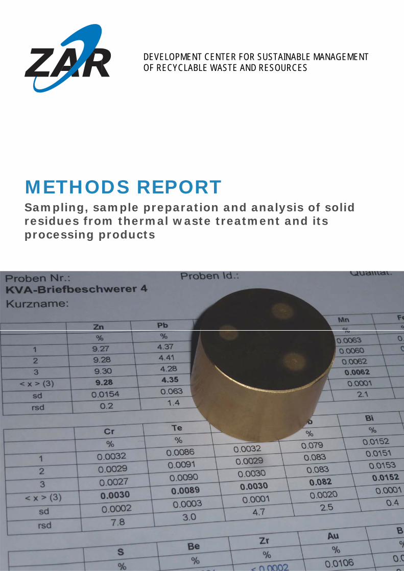
180126 ZAR Sampling methods english final

DEVELOPMENT CENTER FOR SUSTAINABLE MANAGEMENT OF RECYCLABLE WASTE AND RESOURCES

METHODS REPORT Sampling, sample preparation and analysis of solid residues from thermal waste treatment and its processing products

Imprint

Mission and financing The project was implemented on behalf of AWEL Zurich (Waste Management and Operations Department) and the Center for Sustainable Management of Recyclable Waste and Resources (ZAR) in Hinwil. The project was supported through the donation of services by the contractors.

Senior Project Management (POL): Dr. Leo Morf, AWEL Zurich, Waste Management and Operations Department, Waste Management Section, Head of Thermal Waste Treatment Subdivision, Chairman of the Technical Advisory Board of the Center for Sustainable Management of Recyclable Waste and Resources (ZAR), Hinwil

Subdivision Project Managers Rolf Gloor, Managing Director of Bachema AG, Schlieren Stefan Skutan, on behalf of Bachema AG, Schlieren

Project Support Franz Adam, Department Head, Waste Management and Operations Department, AWEL, Canton of Zurich Elmar Kuhn, Waste Management Section Head, Waste Management and Operations Department, AWEL Canton of Zurich Daniel Böni, Managing Director, Center for Sustainable Management of Recyclable Waste and Resources (ZAR) in Hinwil Fabian Di Lorenzo, Center for Sustainable Management of Recyclable Waste and Resources (ZAR) in Hinwil.

Authors of the Methods Report Stefan Skutan and Rolf Gloor, with support from Dr. Leo Morf Acknowledgements: The English version was supported by Hitachi Zosen INOVA, a donator of ZAR.

© March, 2014, English version January 2018

Contents

Preface................................................................................................................................. 1

Part A: Sampling and sample division ................................................................................... 3

1 Selection of access point(s) for sampling ........................................................................ 4

2 Sample numbers and sample masses ............................................................................. 6

2.1 Number of samples ............................................................................................................ 6

2.2 Sample masses ................................................................................................................... 7

2.3 Number and magnitude of the increments when preparing mixed samples ..................... 7

3 Sampling techniques ...................................................................................................... 9

3.1 Collection from free‐falling material flows ......................................................................... 9

3.2 Collection from a conveyor system .................................................................................... 10

3.3 Sampling from heaps and containers, e.g., Big Bags .......................................................... 10

4 Sample division ............................................................................................................. 13 ..

4.1 Ripple divider ..................................................................................................................... 13

4.2 Rotary and other automatic dividers ................................................................................. 13

4.3 Incremental scooping ........................................................................................................ 14

Part B: Determination methods ........................................................................................... 15

5 Determination of iron and non‐ferrous metal particulates in MWIP bottom ashes (fractions) ..... 16

5.1 Determination of iron and non‐ferrous metal particulates > 1 mm in MWIP bottom ashes (fractions) via on‐site preparation using a vibratory roller.............................................. 16

5.2 Determination of iron and non‐ferrous metal particulates in MWIP bottom ashes (fractions) using laboratory preparations ("BAFU method") ............................................................ 20

5.3 Determination of iron and non‐ferrous metal particulates in MWIP bottom ashes (fractions) < 1 mm (laboratory determination)................................................................................ 21

6 Chemical analysis (total element contents) of MWIP bottom ashes and fly ashes ........................ 22

6.1 Chemical analysis (total element contents) of MWIP bottom ashes (fractions) < 1 mm and MWIP fly ashes………………................................................................................................ 22

6.2 Chemical analysis (total element contents) of MWIP bottom ashes (fractions) up to 8 mm ............ 25

6.3 Chemical analysis (total element contents) of MWIP bottom ashes (fractions) up to 80 mm .......... 28

6.4 Chemical analysis (total element contents) of crude MWIP bottom ashes (total bottom ash, with no particle size limitations) .................................................................... 30

7 Determination of metallic and mineral‐bonded fractions of the total element contents of MWIP bottom ashes (fractions) ............................................................................ 32

8 Determination of scrap iron quality ............................................................................... 34

8.1 Determination of the metal content in scrap iron (purity)................................................. 34

8.1.1 Determination of the metal content in scrap iron using a vibrating roller ..................... 34

8.1.2 Determination of the metal content in scrap iron using a vibrating cup mill, ESSA system, or equivalent type of mill in the laboratory (only samples < 20 mm)........ 35

8.2 Determination of the mass fraction of copper windings, batteries, and other objects in scrap iron..................................................................................................................... 35

8.3 Determination of the copper content in scrap iron .......................................................... 35

9 Determination of the quality of non‐ferrous products ................................................... 37

9.1 Determination of the metal content in non‐ferrous products............................................ 37

9.1.1 Determination of the metal content in non‐ferrous products using a vibrating roller ... 37

9.1.2 Determination of the metal content in non‐ferrous products using a vibrating cup mill, ESSA system (or equivalent type of mill) in the laboratory ..................................... 38

9.1.3 Determination of the metal content in non‐ferrous products of < 1 mm using a needle hammer ............................................................................................................... 39

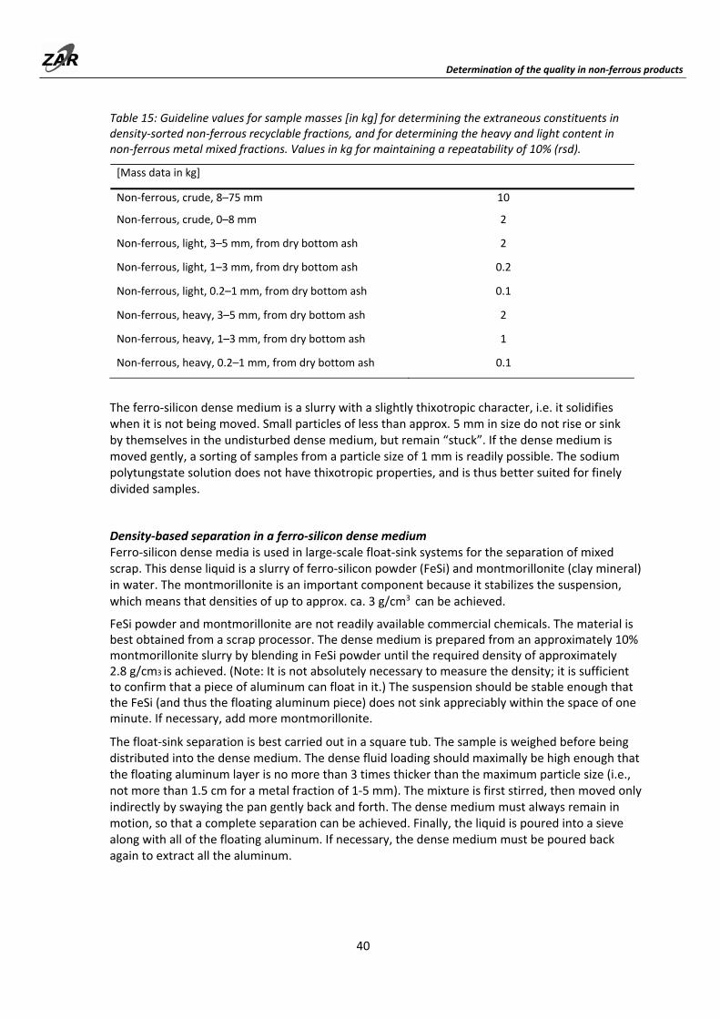
9.2 Determination of impurities in heavy and light non‐ferrous products, and of the heavy and light non‐ferrous content in crude non‐ferrous products ............................. 39

9.3 Chemical analysis (total element contents) of non‐ferrous products................................. 41

9.3.1 Chemical analysis (total element contents) of non‐ferrous heavy products up to 5 mm in a melt ................................................................................................................ 43

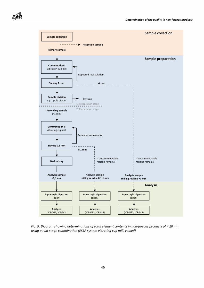
9.3.2 Chemical analysis (total element contents) of non‐ferrous recyclable material fractions up to a particle size of 20 mm through pulverization….................................... 45

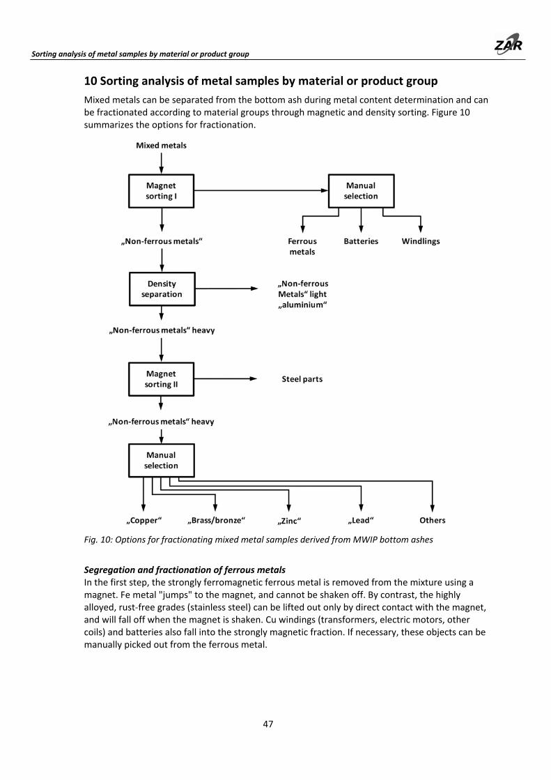
10 Sorting analysis of metal samples according to material groups or product groups ...... 47

11 Digestion and analytical methods for ready‐prepared analytical samples…................... 50

11.1 Determination of total element contents in analytical samples ...................................... 50

11.1.1 Total element content determinations for mineral materials by complete digestion and measurement using ICP‐OES or ICP‐MS .................................................... 50

11.1.2 Total element content determinations for metallic samples by digestion in aqua regia and measurement using ICP‐OES or ICP‐MS................................................... 51

11.2 Determination of metallic aluminums through hydrogen evolution ............................... 51

Glossary ............................................................................................................................... 53

Cited standards .................................................................................................................... 53

Cited literature ..................................................................................................................... 54

Preface

1

Preface

For materials that are significant for economic reasons (e.g., lead or copper), the question of their actual content in geological deposits or in cargoes of ores on freighters has been a matter of interest since the advent of industrial processing of geogenic raw materials. Investment decisions in the mining industry, or raw material delivery prices, have always depended on the results of investigations into the content of the substances that determine the value of the goods. It has long been known that the precision of an analytical result, whether in the exploration of a deposit or the characterization of a ship's cargo, is less dependent on the actual analytical modalities (high‐precision gravimetric methods or high‐resolution, accurate analytical instruments) than on the question of representative sampling.

For this reason, reliable and accurate sampling and sample processing techniques were developed early on, particularly in connection with the extraction of ores, but also in material‐ and capital‐intensive industries, along with the devising of principles for statistical sampling. In doing so, it was necessary to meet the requirements with regard to the amounts, sizes, and frequencies of sampling as a function of (1) the investigated materials, (2) the parameter of interest, and (3) the requirement for the result (uncertainty). Morf (1998) provides a review of the design‐ and model‐based sampling theories already developed by the middle of the last century, as well as combinations thereof (for example, Gy's sampling theory), with references to published sources.

In the past, a large proportion of the substances extracted from geogenic deposits are to be found in the material inventory of industrialized countries, whether it be in infrastructure, consumer or investment goods . It shouldn’t be surprising that waste flows contain potentially recyclable materials that warrant the development of technologies for their utilization. Similar to geogenic raw materials, these resources should be "explored" using suitable testing procedures, and the finished preparation products (such as metal fractions from municipal solid waste incineration plant MWIP bottom ashes) derived therefrom should be considered for commercialization.

Many of the (occasionally valuable) substances contained in the products are harmful if released into the environment. Thus in comparison with the economic potential, avoiding potential ecological harm has been an even stronger justification for chemical waste analysis. The high standards customary in the raw material sector were not initially applied for waste analysis, probably due to the extreme heterogeneity and adverse properties of the samples, which complicate sample preparation. The adaptation of sampling theory applications to problems in waste management was not considered until only a few years ago. Guidelines for defining the minimum requirements for sampling and processing, or approaches to sampling plans, have so far been rather tentative and further development has not been consistently pursued. This contrasts with the fact that waste volumes, as well as the recyclable and pollutant contents in that waste, began to increase rapidly about fifty years ago. This is quite amazing when one considers the consequences, as was systematically presented by Pitard (1998) already back in the 1980s (Figure 1).

Preface

2

Fig. 1: Dependence of analysis results on sample mass (this relationship is valid when only a few samples are analyzed for each test)

The graph (adapted from Pitard, 1998) shows very clearly what happens when the sample quantities collected to determine the content of a substance of interest within a bulk heterogeneous product (for example, a yearly production volume) are too small. This leads to the true (unknown) content being systematically underestimated (without any indication to the contrary). Statistically speaking, analyzing several samples that are too small results in a large range of error, especially in combination with outlier elimination, and supports erroneous conclusions about the mean substance content – a systematic deviation that gives results near the background content instead of a higher, true value. Combined with potential errors due to incorrect sampling techniques and inadequate sample preparation (as may arise from "simplifications" in both steps), this can lead to serious errors in the assessment of the quantities of pollutants or recyclable materials, and thus hampers the estimation of both ecological risks and economic opportunities.

Our modern, highly‐developed society demands ever more complex products with more and more components; these include not only valuable, recyclable materials (e.g., precious metals, rare earths), but also increasing amounts of new, potential pollutants (e.g., flame retardants, nanomaterials). This is why reliable, accurate methods for sampling, sample processing, and analysis are more in demand in the waste and resource management fields (as well as urban mining activities) than ever before.

To ensure and improve reliable quality assessments of residues from thermal waste treatment, but also to determine the economically and ecologically interesting potential of valuable recyclable materials more reliably, ZAR has worked closely together with BACHEMA and with support from the canton of Zurich to optimize the respective methods involved. Following intensive further development of individual procedures over the last nine years, this Methods Report represents the current state of the art in terms of knowledge of practical methods ranging across the entire spectrum of residual fractions from thermal waste treatment. This knowledge shall now be made available for routine use in the field.

I would like to express my thanks to all of those involved for their commitment to this effort.

Dr. Leo Simon Morf

Part A: Sampling and sample division

3

Part A: Sampling and sample division

Every test begins with sampling. The goal is to obtain a sample that is as small as possible while still being representative of the whole. Here, “representative” means that the sample has the "same" composition as the bulk quantity that is to be characterized. The magnitude of permitted deviation (the "sampling error") depends on the task definition of the analyses to be run. Practically speaking, the composition of the sample can deviate only so far from the composition of the bulk quantity that it does not impair the significance of the analysis for the given task definition.

A sample can be thought of as an "information carrier", and the "extraction" of this information is facilitated by sample preparation and analysis. It is not possible to determine from the analysis results whether the information contained in the sample correctly reflects that of the bulk quantity (i.e., if the sample is representative). The samples cannot be guaranteed to be representative unless all criteria for "correct" sampling are complied with. After the fact verification of representative sampling is not possible unless the entire bulk quantity has been stored and sampling can be repeated. For this reason, the sampling procedures must be given a high priority. The occasionally intensive effort that is necessary for correct implementation should be made whenever possible.

"Correct sampling" is defined as part of Gy's sampling theory and many aspects of its practical implementation have already been described (for a detailed description, see Gy, 1992). An attempt has been made in the following to summarize the essentials of the approach with respect to the distinctive features of municipal solid waste incineration plant (MWIP) combustion products.

Sampling error is basically made up of two components, one of them systematic and one of them random. Systematic errors result from a poor, “incorrect” sampling system. A system is “correct” when it is ensured that each particle of the bulk quantity has the same probability of being in the sample. This is not the case if, for example, "samples" are only taken from the surface of an aggregate material surface, or when a material stream is not sampled uniformly across its entire cross‐section. Systematic errors thus arise when something has actually been done systematically incorrectly. Random sampling errors, on the other hand, are a direct consequence of the heterogeneity of the material and will always occur, even if the sampling is done "correctly". (It is for this reason that the expression “correct sampling error” can also be used for random error.) The term “error” is used here in its meaning within the field of statistics, commonly understood as a “deviation”, and does not necessarily mean that something was done incorrectly. Random sampling error is dependent on the heterogeneity of the bulk material as well as on sample mass and, in the case of mixed samples, the number of increments (sub‐quantities) that are combined to make up a mixed sample.

(Note: As mentioned in the preface, an analysis system that employs correct sampling techniques but includes a low number of samples of very insufficient size, especially in combination with outlier elimination, can lead to findings which are seriously and systematically too low. This is another type of system error. The analysis system will then systematically produce extremely skewed (left‐hand tail) measured value distributions. The individual values from such distributions, or the mean values from a small number of individual values, have no significance with regard to the true average content, and in the vast majority of cases are far too low.

The material in question is correctly regarded as being highly heterogeneous. Nevertheless, it is still possible to keep the sampling error small. Two factors essentially determine the heterogeneity of the bulk material: the diversity of the individual particles of which the material is composed ("constitutional heterogeneity"), and how the various components or individual particles are distributed within the bulk material ("distribution heterogeneity").

Selection of access point(s) for sampling

4

An extreme case of constitutional heterogeneity is, for example, gold in MWIP bottom ash. The majority of the Au content is found in few, highly concentrated Au particles, while all of the other bottom ash particles contain virtually no Au. On the other hand, for example, the constitutional heterogeneity with respect to Al is much smaller. Although there are also highly concentrated Al metal particles, first of all they are much more densely dispersed than Au particles, and second of all many mineral bottom ash constituents contain Al in chemically bonded form. Distribution heterogeneity, in turn, refers to the uneven distributions of components in space (e.g., in heaps formed by pouring a variety of materials on top of one another) or over time (e.g., changes in bottom ash composition with varying waste composition). The effects on sampling error due to both of these heterogeneity factors can be controlled. The random, "fundamental errors" resulting from constitutional heterogeneity in the sampling can be controlled through sample mass. The sampling error that results from distribution heterogeneity can be controlled through the number of individual samples ("increments") that are combined to make up a mixed sample. This document specifies guideline values for (parameter‐dependent) minimum sample masses and increment numbers for many tasks.

The first step in sampling is to determine the sampling mass of the "primary samples". The primary sample mass depends solely on the type of material (constitutional heterogeneity) and on the analytical parameters (respective reference values listed in part B). Selecting a suitable "access point" is the next step. In practice, it is often difficult to gain access to the material (often a material stream) in such a way that samples of the desired quantity can be collected properly (sampling techniques, Chapter 3). The number of increments from among which the primary samples are finally mixed depends on the mixing status of the material at the access point. The required number is determined from an estimate of distribution heterogeneity (Section 2.3). It is not always possible to collect increments of the desired mass. Particularly when sampling crude bottom ashs, considerably larger quantities must be collected because the sampling technique does not accommodate small quantities. In such cases, the primary samples must be divided on site or in the laboratory before actual sample preparation begins. In principle, each sample division should be classified as a new "sampling" ("secondary sampling"). Each sample division is thus as critical as the primary sampling itself. For these reasons, sample division is discussed here in conjunction with sampling.

1 Selection of access point(s) for sampling

Access point can be understood in two ways: first of all, it can be the specific location where the sampling takes place, e.g., a specific point on a conveyor line at which material can be collected, and second of all ‐and in terms of logistics ‐ it can be the place in the transport, treatment, or recycling chain at which the sample collection is able to be performed. Examples of access points include:

– discharge or transfer points in conveyor systems (e.g., conveyor belts) – easily accessible conveyor belts that can be temporarily halted (for scooping up sample

material from the belt) – EMERGENCY EXIT points – material movement in the rearrangement of heaps

The access point must meet the following requirements in each case without fail:

– access to the entire quantity to be characterized must be possible,

Selection of access point(s) for sampling

5

– a technique for proper collection must be deployable or installed.

In addition, it is recommended that the selected access point be one at which:

– collection of multiple increments can be implemented simply and with little effort; and – variability in the material is low, i.e., the mixing status is high.

Achievable accuracy will not however be limited if the last point cannot be met. High variability can be compensated for by having a high number of increments.

The requirement that each fraction of the bulk material must be accessible, i.e., that each particle has the same chance of being included in the sample, is the basic principle of proper sampling. This requirement can be most easily met when material flows are sampled. In a material stream, the bulk material presents itself as a linear belt that is accessible at any point in the same manner, and from which a portion (increment) can be “carved out”. The increments of material can be collected for a certain period of time, e.g., at a discharge point in the conveyor belt, or the conveyor belt can be turned off and a portion thereof is completely removed. When the collection times at which increments are taken are selected randomly, the probability for all the particles to being included in the sample is equal. This fulfills the requirement for proper sampling. If it can be ensured that cyclic fluctuations are absent and only random fluctuations occur in the material flow, then collection at fixed intervals is equivalent to the random selection of collection times. In principle, however, it is advisable to avoid fixed intervals, or to ensure that the intervals are not exactly the same. If the material composition changes periodically and the sampling intervals inadvertently coincide with the fluctuation periods, systematic sampling errors will occur.

For each access point considered, it must be clarified whether periodic fluctuations or exceptional status events can occur, and whether the corresponding variability is higher or lower relative to other candidate access points. The following effects can cause such periodic fluctuations:

– periodic delivery/processing of special wastes (e.g., in weekly intervals), – periodic changes in the operational status, e.g. during cleaning or maintenance work, – discontinuous conveyor systems, e.g., grate advancement, ram bottom ash extractor, etc.

It is advisable to conduct observations at a suitable access point over a period of time to determine whether the material flow changes conspicuously in terms of quantity or particle size distribution. If a batch‐feeding conveyor system is installed, the particle size of the material usually changes as a function of the flow rate. At the beginning of a batch, a large quantity is conveyed; this generally contains a large amount of coarse material, whereas later in the run the "after‐flow" is comprised mainly of finer material. To compare variability at different access points, it is sufficient to assess the uniformity of the quantity flow and particle size distribution (possibly the color or the frequency of metals or of other conspicuous components in the mixture) through simple observation.

Cyclical fluctuations in the quantity of material or composition are not in themselves a problem, but it is absolutely necessary for the sampling times to be set at random intervals instead of fixed ones. Otherwise, an unintentional synchronization between the conveyor and the sampling rhythm could occur, and systematic sampling errors would be the result.

Sample numbers and sample

6

The intermixing status of the bulk material changes when the material is piled up in heaps or loaded into containers. For example, this segregating effect is particularly strong when an MWIP bottom ash falls from a high discharge point and forms a heap below (e.g., in a bottom ash bin). Such heaps consist mainly of fine material in the core, because the coarser material rolls well, and accumulates on the flanks of the heap. Generally speaking, the broader the spectrum of particle sizes and shapes, the greater the segregation tendency. When these kinds of heaps are excavated for transport, older and younger materials will become mixed (which is desirable, since it reduces variability), but the resulting segregation according to particle size creates new variability in the discharge stream (for example at the loading site after a bottom ash bin). The described effects also occur, even if much less pronounced, when filling and emptying silos with free‐flowing material.

As a rule, undisturbed piles cannot be sampled, since not all areas are accessible (see Section 3.3). Heaps can be relocated, or spread to allow access to the entire mass of material. During a transfer, the material is in a stream that can be properly sampled. Heaps that are not too large can be spread out, and increments can be taken from them as from a mixing bed (see Fig. 2, page 12). Wherever possible, sample collection from heaps should be avoided, and an access point should be selected where the material can be sampled as a stream.

Selection of the access point must be done in a timely manner, so that the sampling carried out at the most suitable location can be technically beyond question. Proper collection of the samples must be done without compromise. Unfortunately, having sample collection points in conveyor systems is the exception rather than the rule. Under certain circumstances, alterations are necessary to create a possible access point.

2 Sample numbers and masses

2.1 Number of samples

The procedures for sampling, sample preparation, and analysis described in this document provide results with small or moderate variance. Accurate determinations are therefore also possible with just a few or even with only one (mixed) sample. Since, as a rule, sample collection from a material stream cannot be repeated, at least two (mixed) samples must be generated. If there is only one, the risk is too great of not having a reliable sample, e.g., if a mistake occurred during sample preparation. The number of increments should be multiplied accordingly for generating several mixed samples. The successively extracted increments are assigned to the mixed samples alternately in the case of two mixed samples, and in rotation in cases of several mixed samples.

Examination of a single sample (and setting another one aside) is sufficient if

– sample collection at the selected access point has already been successfully tested, – the sample mass data has been tested and – a tested method of determination (from Part B) was used.

Note: Sample collection or sample mass data qualify as having been “tested” when the results from two samples yield the desired match (e.g., less than 10% relative standard deviation, rsd) in at least two consecutive samples from the same access point.


7

The determination uncertainty cannot be derived from the analysis results of individual determinations. However, the determination uncertainty achieved under normal conditions can be indicated for the determination methods themselves. The data are empirical values for the respective materials and sample masses.

In the case of materials for which no tested sample masses or preparation procedures are specified, at least two samples must be prepared and analyzed.

2.2 Sample masses

The primary sample mass depends solely on the type of material (constitutional heterogeneity) and on the analytical parameters. Sample mass data for the individual analysis tasks can be found for a number of analysis parameters in Part B. For parameters not listed there, sample masses should be adopted from parameters that are expected to be within a similar concentration range. When defining sample masses for materials that do not fall into one of the listed particle size grades, classification according to upper particle size limits is used for orientation.

2.3 Number and magnitude of increments when preparing mixed samples

The distribution heterogeneity is usually unknown. Thus, in most cases, it is not possible to provide more than a rough estimate of the necessary number of increments. Because of the uncertainty, a safety margin must be included in the planning.

No comprehensive studies exist addressing variability between individual increments for MWIP combustion residues. Initial clarifications for MWIP residues were made in Vienna at the end of the 1990s (see: Morf, 1998). Empirical values do however exist that result in low variance in mixed samples:

– 25 or more increments per mixed sample for material streams that "appear uniform", – at least 60 increments per mixed sample for material flows in which quantities and particle

size distributions fluctuate conspicuously.

“Uniform” here means that no conspicuous changes in quantity and visual appearance can be seen. Conspicuously fluctuating material streams include, for example, MWIP bottom ashs directly downstream from the discharge, where the fluctuation is caused by the periodic discharge of the material from the grate and, if need be, intermittently conveying extractors (ram bottom ash extractors).

If, in exceptional cases, the variability is known (in fly ash, for example, where the variance of heavy metal contents between individual increments can be measured relatively easily using XRF), or if worst‐case scenarios are available, the required increment number can be determined from Table 1.


8

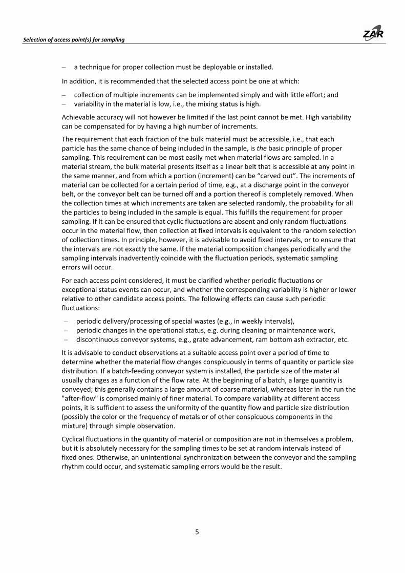
Table 1: Required number of increments per mixed sample as a function of the initial variability in the material and the desired residual variability of the mixed samples. For example: at least 16 increments are necessary to achieve a 5% rsd with an initial of 20%.

Variability in

material (stream)

% rsd

Required residual variability in

the mixed samples [% rsd]

2 5 10 20

10

20

50

100

25 4 1 1

100 16 4 1

625 100 25 6

2500 400 100 25

The size of the increments depends on the sample mass that is required for the respective analysis task. If the necessary sample mass is for example 10 kg, and if 25 increments are used, an average mass per increment of 0.4 kg is called for.

Note: Individual increments may deviate considerably from the calculated target mass if the flow rate at the access point fluctuates greatly. In any case, the access time for collecting an increment must always be the same, regardless of how difficult obtaining the individual increments turns out to be. Under no circumstances should the access time be extended, nor should the access time be shifted if "only a little is coming out".

In some cases, the increments obtained cannot be as small as desired with available sampling techniques. For example, it is difficult to achieve good consistency with brief access times (one second or less) when sampling is performed manually. Also, no small increments on the kg scale can be obtained from very coarse material, e.g., crude MWIP bottom ash. In such cases, the increments must be increased to ensure reliable collection. However, in contrast to the increase in increment size, the number of increments themselves may not be reduced. Primary samples that are too large can subsequently be divided to obtain the originally intended sample mass if this can be accomplished in the proper manner. In the case of a free‐flowing material, it is recommended to increase the incremental size by a multiple of two so that the primary samples can be easily and quickly divided to obtain the originally intended target mass by means of ripple dividers.

Sampling techniques

9

3 Sampling techniques

Various sample collection techniques are described below. Since sampling from free‐falling material flows has the least susceptibility to systematic errors, and furthermore often readily lends itself to automation, it should be preferred over other methods. For all manual sample collection techniques, occupational safety regulations must be observed.

3.1 Sample collection from free‐falling material flows

Suitable access points for this type of sample collection are the discharge points in conveyor belts or other conveying devices, as well as downpipes and the like. In any case, the material flow to be sampled must be in free fall.

Either a collection vessel is passed across the entire breadth of the material flow, or the latter is collected in its entirety for a certain period of time. The sample collection process can be carried out manually or mechanically. The criteria for proper sampling are as follows:

− each access (sample collection process) must last exactly the same length of time and should otherwise be executed in exactly the same manner;

− the entire cross‐section of the falling material flow must be uniformly contacted; each point of the cross‐section must be covered by the collection vessel for the same length of time;

− the material flow must be passed through completely in one direction with a collection vessel during the sample collection process;

– the sampling vessel must either pass through the same cross‐section of the material flow at a uniform speed or,

– if the vessel is to contact the entire cross‐section for an extended period, it is to be moved into and out of the sample collection position at the same speed and in the same direction of movement;

– the vessel must be large enough so that it is never overfilled, meaning that all of the material that falls through the cross‐section opening will be collected in its entirety;

– no sample material should be lost by back‐splashing from the vessel; – the edges of the vessel must be so narrow that no material can accumulate on them.

A detailed evaluation of various access systems can be found in Gy (1992).

Automatic sample collectors have a long and proven history in the raw material industry, and are available from several companies. The machines must accommodate in each case the properties of the material to be sampled. Automatic samplers that are conventionally designed for free‐flowing bulk solids are sometimes susceptible to interference if the material is sticky or if it contains for example filaments that can remain behind in the machine. Prior to procurement, the instrument should be checked very carefully to determine whether an automatic sampler for the specific application fulfills the above‐mentioned requirements for proper sample collection and whether the system can be operated without malfunction.

Determination of access time The access time must be set so that, on average, the target mass per increment is reliably achieved (or exceeded). The average flow rate in kg/s must be known to calculate the access time. The flow rate can be determined during a sampling test run. Estimates can also be calculated from the production volume and the hours of operation. If it is detected during a sample collection series that the target sample mass has not been achieved, it is not primarily an access time adjustment that should be implemented, but rather an increase in the number of increments.

Sampling techniques

10

3.2 Collection from a conveyor system

Material lying on a stationary conveyor belt can be classified as a "solidified" material flow. From this flow, the increments for sampling can be “carved out”. A segment is clearly demarcated and removed from the stationary belt in its entirety. The criteria to be met are:

− sample collection must extend across the entire width of the conveyor belt;

− the "cuts", i.e., the boundaries before and after the sample material must be parallel, and must have the same distance for each collection;

– the boundaries must be designed as sharp cuts;

− the sample, i.e., the material within the boundaries, must be removed completely from the conveyor belt.

"Sample delimination pins" can be placed in the material to ensure a parallel separation at a constant distance. Clear boundaries are made difficult with coarse material, especially when bulky items such as filaments or metal sheets are intermixed. Sampling from the freely falling material flow is preferred with these kinds of material flows.

Note: Vibro chutes are not suitable for this type of sampling! Vibro chutes do not transport all particles equally quickly, which means that the composition in the chute is distorted. Particles that migrate slowly are overrepresented in the chute and those that migrate rapidly are underrepresented.

Determination of section length This determination is carried out analogously to the determination of the access time for the sampling of freely falling material flows (Section 3.1). Optimally, the average conveyor belt loading (kg/m) is determined over the course of a test sampling. The material flow rate and belt speed must be known if the loading is to be calculated.

3.3 Sampling from heaps and containers, e.g., Big Bags

From the point of view of sampling, a heap is a three‐dimensional quantity of bulk material (in contrast to a "quasi‐linear" material flow). Proper sample collection requires that material be taken at randomly selected positions from within the volume of the heap. The increments must be sharply delineated within the original configuration, and must all have the same volume. This type of sampling is feasible only if a heap is solid to the extent that the material does not slide during the excavation and removal of the increments. However, sampling in this system would involve the same effort as the complete rearrangement of the heap.

A better option for collecting samples from heaps is to relocate them in their entirety, and to conduct the sampling from the resulting "material flow". Ideally, the material should be run via a conveyor device to enable actual sampling of a material stream, as described in Section 3.1. If this is not possible, individual shovel loads can be extracted as increments over the course of the entire relocation process. Machines with a small shovel should be used to keep the primary sample mass as small as possible. In most cases, however, it will still be necessary to divide the primary samples or relocate the primary samples on a smaller scale, and then to re‐sample from them.

The same principles can be applied to smaller heaps that can be shoveled manually. This type of sampling is however error‐prone and should be used only in exceptional cases. The sample collector will involuntarily strive to select "average material" for the samples, and this can easily result in a systematic sampling error.

Sampling techniques

11

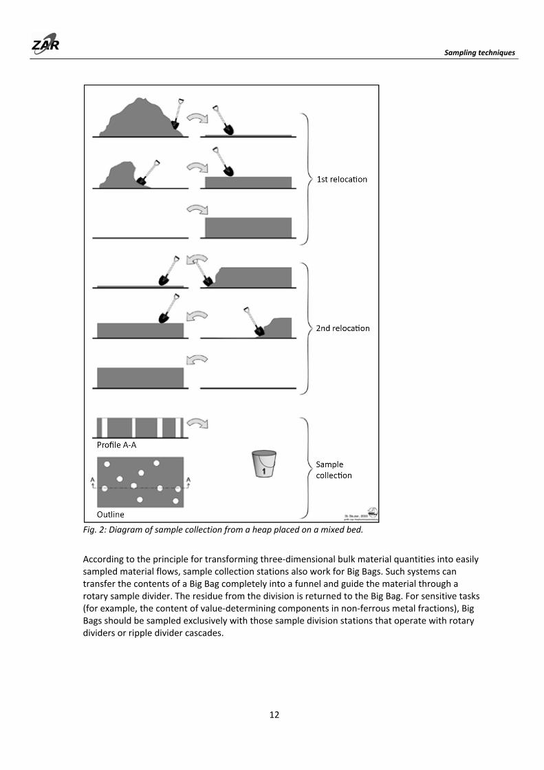
One option for extracting samples from a heap is to spread out the heap in a thin layer and to "peg out" increments from the surface. In cases of poor mixing statuses, the material itself can still be mixed to a greater extent prior to the removal of the increments by constructing a "mixing bed". Fig. 2 illustrates the procedure, including a two‐step thorough mixing. The material from the heap is distributed shovel by shovel onto a smooth substratum. Each shovel load should be distributed widely. The starting and ending points of the distribution of the individual portions should be different in each case. Overall, a rectangular mixing bed is to be constructed from the entire bulk material. To achieve complete and thorough mixing, the first mixing bed can be excavated from one side and be layered in the same way onto a second mixing bed. It is only from this second mixing bed that the increments are removed. Vertical holes are excavated at a minimum of five points for this purpose. (If a heap is only to be taken apart, i.e., without mixing, at least 25 increments should be removed.) The excavation can be done well using a mason’s trowel or a sampling scoop. It is important that all holes reach down to the bottom. The holes must be made vertically downwards, and the ground must be cleaned out well. If the material is in movement afterwards, pipe sections or square frames must be pressed into the mixing bed to delineate the increments sharply from the rest.

The division of heaps by "coning and quartering" should be avoided if possible, especially when dealing with a material that easily becomes segregated or contains bulky parts that make the quartering of the coning more difficult. For samples that are prone to segregation, each scoopful should be placed on the cone from a different side, so that the (de‐)mixing status of the cone is rotationally symmetrical.

Sampling techniques

12

Fig. 2: Diagram of sample collection from a heap placed on a mixed bed. According to the principle for transforming three‐dimensional bulk material quantities into easily sampled material flows, sample collection stations also work for Big Bags. Such systems can transfer the contents of a Big Bag completely into a funnel and guide the material through a rotary sample divider. The residue from the division is returned to the Big Bag. For sensitive tasks (for example, the content of value‐determining components in non‐ferrous metal fractions), Big Bags should be sampled exclusively with those sample division stations that operate with rotary dividers or ripple divider cascades.

Sample

13

4 Sample division

In principle, sample division is also a type of "sampling", and is therefore subject to the same principles and sources of error. Divided samples can therefore be considered as “secondary samples”, and following an additional dividing step, as “tertiary samples”, etc. The mass of a divided sample should not be less than the applicable minimum sample mass for the material in its current state with regard to constitutional heterogeneity.

The sample division techniques used must ensure that even samples with a high degree of segregation will be "correctly" divided. With few exceptions, properly functioning sample division techniques must always be applied when sample masses are reduced. Exceptions can be made only for finely pulverized materials for which thorough mixing can be relied upon, and for cohesive, wet materials that do not self‐segregate.

The following techniques are generally suitable for carrying out sample division:

4.1 Ripple divider

The selection of an appropriate ripple divider depends on the particle size of the sample material. The shaft width must be at least three times the diameter of the largest particle so that the divider doesn’t become clogged, but should not exceed twice that value. In addition, the design of the divider is crucial, and not all commercial devices are properly constructed. The requirements for ripple dividers are as follows:

– same number of shafts in both discharge directions; – at least 14 shafts; – all shafts, including the outermost ones, have the same width; – external walls of the outermost shafts are vertically elongated (not constructed in the

form of a "funnel"); and, – feed container is just large enough to cover the width of all shafts.

The sample material must be supplied to the divider using the associated feeder hopper or a wide shovel. The feeder hopper or shovel must extend exactly across the entire width of the divider, i.e., across all the shafts. Under no circumstances may the material be poured directly from a bucket into the divider or "distributed" over the shafts with a grain shovel (or the like). The material must fall freely, usually vertically into the shafts. In any case, the flowing material must not become stuck on the divider wall that is positioned opposite the feeder hopper. (Some dividers are equipped with a device for swiveling up and emptying the feeder hopper. Such dividers always operate flawlessly, but cleaning them is more complex than with simpler models.) Segregation of the material during filling of the feeder hopper is of no relevance. Any filaments or the like that remain attached to the partition walls between the shafts must be removed immediately so that the material flow remains undisturbed. These removed filaments are then distributed alternately into the two partial samples.

4.2 Rotary and other automatic dividers

Rotary dividers operate according to the principle of sample collection from the material flow, as described in Section 3.1. An increment for the secondary sample is generated with each revolution. All requirements listed in Section 3.1 for sampling from material flows must also be fulfilled when working with rotary dividers.

Sample

14

In addition, the devices must be operated in such a way as to obtain a sufficient number of increments. Small samples must be passed through slowly enough that the outlet for collecting partial samples is operated at least 25 times.

Rotary dividers can be used only if the material is free‐flowing. They are unsuitable for materials that contain filaments or other bulky particles.

4.3 Incremental scooping

This sample division method is used when the samples are not suitable for ripple dividers or rotary dividers, e.g., because they are wet and not free‐flowing, or when no divider of the required size is available. Incremental scooping is preferable to dividing by coning and quartering, especially when the material is susceptible to segregation or contains bulky portions that makes quartering the cones difficult.

The sample volume is turned over completely and is divided into two or more equal‐sized portions. The portion that is to be processed as a sample must be chosen randomly after being turned over. The shovel used must be of a size such that each partial sample is at least the size of 25 shovels. Shovel loads from the sample to be divided are assigned in turn to first one and then to the other partial sample. When divided into more than two partial quantities, the shovel loads are assigned in round‐robin sequence. During the shoveling, no consideration should be given to any visible heterogeneity or variability in the material. It is important to ensure that all shovel loads are approximately the same size. Under no circumstances should any attempt be made to compensate for perceived non‐uniformity of the material.

Part B: Determination

15

Part B: Determination methods

This section describes determination methods for various parameters that are relevant for individual material types. The methods have been tested in the manner described.

The focus of the descriptions is on sample preparation. Justification for classification according to particle size is based on the dependence of the minimum sample masses on particle size, which means that, starting from certain particle sizes, there will be a need for further sample processing steps with subsequent sample division. The particle size limits used in the preparation schemes here are based on current experience, and are not to be regarded as strict requirements.

Determination of iron and non‐ferrous metal particulates of MWIP b h (f i )

16

5 Determination of iron and non‐ferrous metal particulates of MWIP bottom ashes (fractions)

These analytical procedures are used to determine the content of granulates and lumps of iron and non‐ferrous metals, as well as stainless steel. If necessary, non‐ferrous metals can be divided into light non‐ferrous (e.g. aluminum etc. ) and heavy non‐ferrous (mixture of heavy non‐ferrous metals such as zinc, lead, tin, and precious metals). The metals from the bottom ash samples are separated, sorted, and weighed. The separation is carried out according to the established principle of selective comminution of the mineral components ("BAFU method", see BAFU, 2013). The metals are not broken down but are only released, and deformed if necessary, and can thus be removed from the samples as oversized particles.

MWIP bottom ashes contain not only more‐or‐less contaminated, "free" metal particles or pieces, but also those that are included in bottom ash particles or chunks. The methods described also include these included metals. Only the content of "free" metal particles or pieces can be determined by approximation by screening the samples into narrow particle size ranges prior to metal separation, and then processing these individually. The respectively smaller metal particles from inclusions are then not detected. Example: A bottom ash fraction of 1‐5 mm is sieved into particle size classes 1‐2 mm, 2‐4 mm, and 4‐5 mm. The fractions are individually fractionated further, whereby the original 4‐5 mm fraction is sieved off at 4 mm, the 2‐4 mm fraction at 2 mm, and the 1‐2 mm fraction at 1 mm. In this way, the small metal particles that have been released from larger bottom ash particles are not detected. For example, the metal particles < 4 mm, which were released from the 4‐5 mm bottom ash particle fraction, fall through the 4 mm screen and are not sifted out. The separated metal portion from this procedure contains only metal particles which had actually been contained as free metal particles in the original sample.

5.1 Determination of iron and non‐ferrous metal particulates > 1 mm of MWIP bottom ashes (fractions) through on‐site preparation using a vibrating roller

This method of determination is primarily intended for use at the sampling site. No actual laboratory equipment is required. The necessary equipment includes a hand‐held vibrating roller, with at least 300 kg in the case of a single‐roll roller or 600 kg for a double roller, a steel plate with a minimum thickness of 5 mm and ideally 6 x 1.5 m in size, as well as hand sieves and a tub suitable for wet screening. Either wet or dry samples can be processed.

Sample collection must be carried out at a suitable access point using proper sampling technique (see Part A). Prior to metal content determination, crude MWIP bottom ashes are often classified in order to be able to determine the particle size distribution of the bottom ash and the metal contents in the individual particle size ranges. Wet bottom ash can be sifted in its original weture state from sieve mesh size of about 20 mm with good selectivity. Finer screening of wet samples must be carried out in the wet state. In wet screening, either the material can be sprayed with water during sieving (sprayer), or it can be sieved in a water bath. In principle, dry bottom ash can be worked dry if dust formation does not impair worker safety. Otherwise, the material can be wetened or wetted before being worked.

Table 2 shows the sample masses required for determination. If the metals have a broader particle size range, e.g., 1‐20 mm, start with the sample mass specified for bottom ash of 10‐20 mm. Metal separation is then carried out in several stages. After a sieving, the sample mass can be reduced according to the particle size achieved. The metal separation works best when the particle size gradation is not too broad. From stage to stage, the particle size should be approximately halved, and not reduced to less than one‐third.

Determination of iron and non‐ferrous metal particulates of MWIP bottom

17

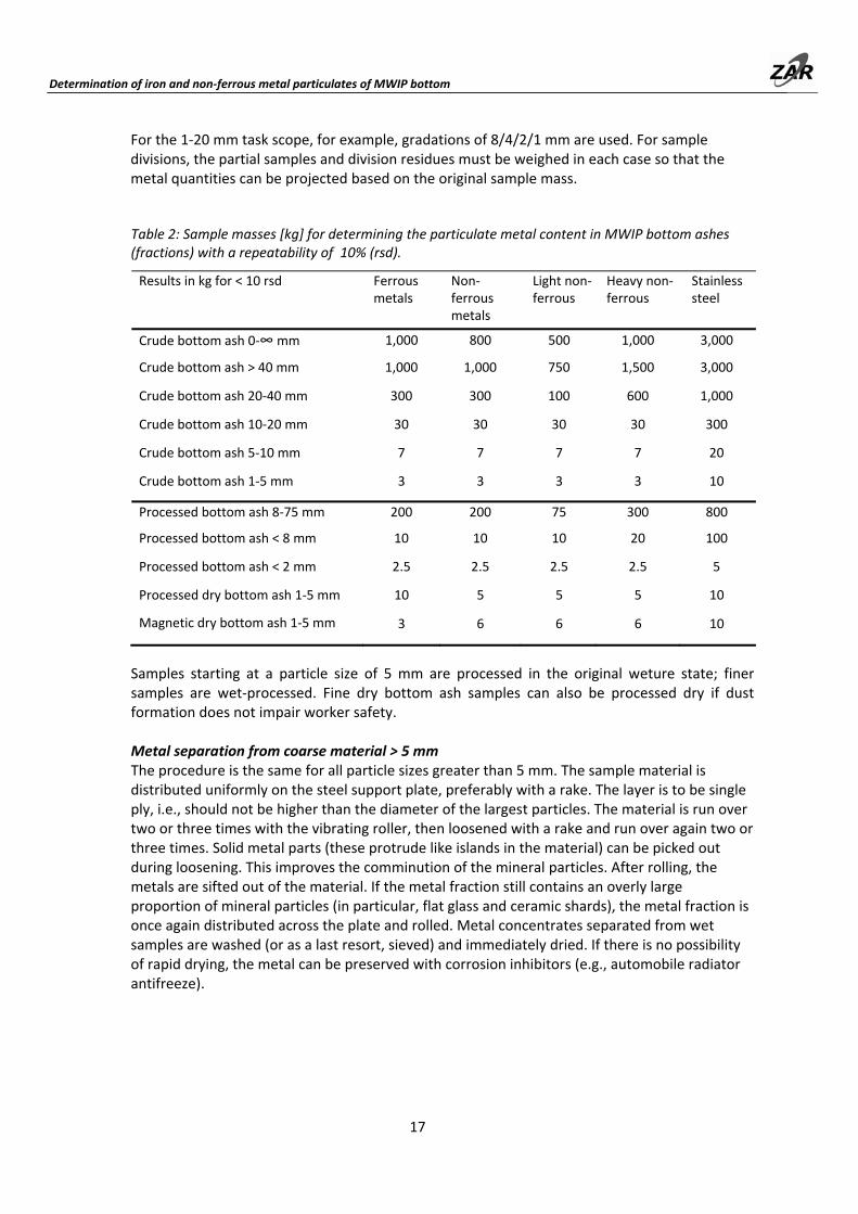
For the 1‐20 mm task scope, for example, gradations of 8/4/2/1 mm are used. For sample divisions, the partial samples and division residues must be weighed in each case so that the metal quantities can be projected based on the original sample mass.

Table 2: Sample masses [kg] for determining the particulate metal content in MWIP bottom ashes (fractions) with a repeatability of 10% (rsd).

Results in kg for < 10 rsd Ferrous metals

Non‐ferrous metals

Light non‐ferrous

Heavy non‐ferrous

Stainless steel

Crude bottom ash 0‐∞ mm 1,000 800 500 1,000 3,000

Crude bottom ash > 40 mm 1,000 1,000 750 1,500 3,000

Crude bottom ash 20‐40 mm 300 300 100 600 1,000

Crude bottom ash 10‐20 mm 30 30 30 30 300



Processed bottom ash 8‐75 mm 200 200 75 300 800

Processed bottom ash < 8 mm 10 10 10 20 100

Processed bottom ash < 2 mm 2.5 2.5 2.5 2.5 5

Processed dry bottom ash 1‐5 mm 10 5 5 5 10

Magnetic dry bottom ash 1‐5 mm

3 6 6 6 10

Samples starting at a particle size of 5 mm are processed in the original weture state; finer samples are wet‐processed. Fine dry bottom ash samples can also be processed dry if dust formation does not impair worker safety.

Metal separation from coarse material > 5 mm The procedure is the same for all particle sizes greater than 5 mm. The sample material is distributed uniformly on the steel support plate, preferably with a rake. The layer is to be single ply, i.e., should not be higher than the diameter of the largest particles. The material is run over two or three times with the vibrating roller, then loosened with a rake and run over again two or three times. Solid metal parts (these protrude like islands in the material) can be picked out during loosening. This improves the comminution of the mineral particles. After rolling, the metals are sifted out of the material. If the metal fraction still contains an overly large proportion of mineral particles (in particular, flat glass and ceramic shards), the metal fraction is once again distributed across the plate and rolled. Metal concentrates separated from wet samples are washed (or as a last resort, sieved) and immediately dried. If there is no possibility of rapid drying, the metal can be preserved with corrosion inhibitors (e.g., automobile radiator antifreeze).

Determination of iron and non‐ferrous metal particulates of MWIP

18

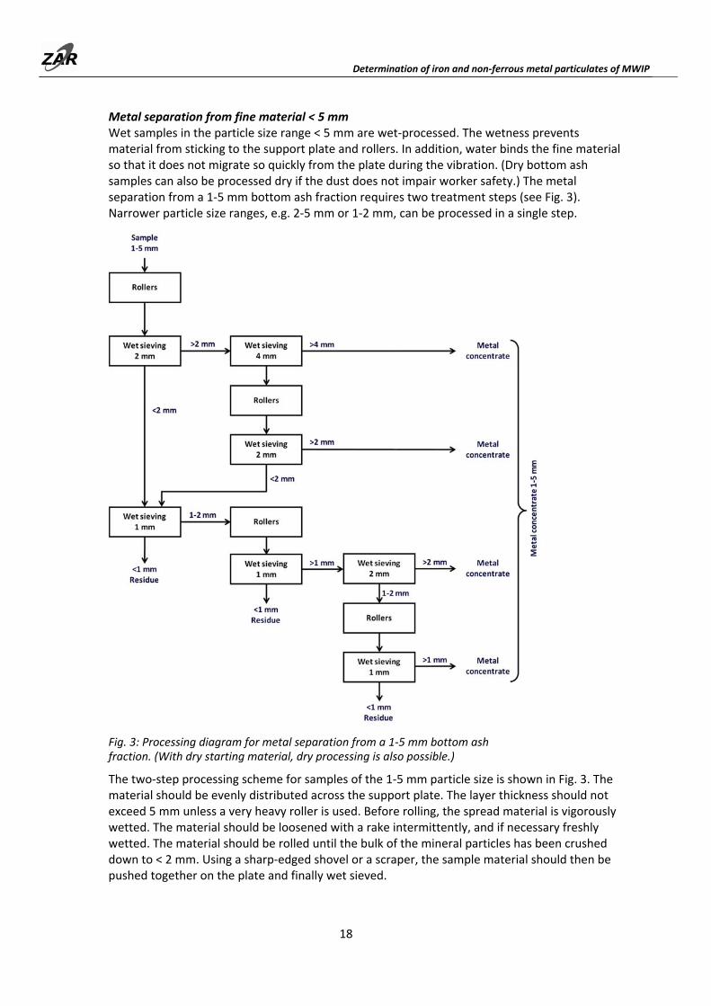
Metal separation from fine material < 5 mm Wet samples in the particle size range < 5 mm are wet‐processed. The wetness prevents material from sticking to the support plate and rollers. In addition, water binds the fine material so that it does not migrate so quickly from the plate during the vibration. (Dry bottom ash samples can also be processed dry if the dust does not impair worker safety.) The metal separation from a 1‐5 mm bottom ash fraction requires two treatment steps (see Fig. 3). Narrower particle size ranges, e.g. 2‐5 mm or 1‐2 mm, can be processed in a single step.

Fig. 3: Processing diagram for metal separation from a 1‐5 mm bottom ash fraction. (With dry starting material, dry processing is also possible.)

The two‐step processing scheme for samples of the 1‐5 mm particle size is shown in Fig. 3. The material should be evenly distributed across the support plate. The layer thickness should not exceed 5 mm unless a very heavy roller is used. Before rolling, the spread material is vigorously wetted. The material should be loosened with a rake intermittently, and if necessary freshly wetted. The material should be rolled until the bulk of the mineral particles has been crushed down to < 2 mm. Using a sharp‐edged shovel or a scraper, the sample material should then be pushed together on the plate and finally wet sieved.

Determination of iron and non‐ferrous metal particulates of MWIP bottom ashes

19

As a rule, the metal concentrate > 2 mm in size from the first sieving still has too much mineral constituent content. For cleaning, it is rolled again and resieved. The effectiveness of the comminution can be improved if, prior to re‐rolling, the largest metal particles are sieved out with a 4 mm sieve. The entire undersized particle portion (< 2 mm) is sieved at 1 mm. This considerably reduces the mass that must be further processed. The procedure for the metal separation from the 1‐2 mm fraction is the same as for the 2‐5 mm processing step. The material is rolled twice. Between the two rolling passes, the already comminuted mineral content < 1 mm in size is screened off and the coarse metal particles are also removed. (Rolling flattens the coarse metal particles.) They then become larger and can therefore be removed by sieving at 2 mm.

Note: The residual fraction < 1 mm is discarded. Clean separation of even finer metals is practically impossible with this technique. If the content of metals < 1 mm in size is to be determined, the residue can be sampled and further examined using the needle hammer method (see Section 5.3). If only the metallic aluminum content in the residual fraction is to be determined, the "hydrogen method" (see Section 11.2) can be applied. In either case, the determination must be made immediately after rolling, or the samples should immediately be dried to stop corrosion of the metallic aluminum. If the samples are stored in the wet state, the metallic aluminum will be lost.


20

5.2 Determination of iron and non‐ferrous metal particulates in MWIP bottom ashes (fractions) using laboratory preparations ("BAFU method")

This method is taken from the BAFU Methods Report “Analysenmethoden im Abfall‐ und Altlastenbereich” (BAFU, 2013 [no English version available]). The diagram in Fig. 4 shows the separation of the metals in the 2‐16 mm range, and reference is made to the detailed description of the procedure from the BAFU Methods Report (page 63 ff.). The metal fraction in the 1‐2 mm range can also be separated according to the same comminution principle using a jaw crusher with subsequent sieving.

Fig. 4: Diagram of the determination method for metal particulates in MWIP bottom ashes (=slag) from the BAFU Methods Report. (Source: BAFU, 2013)

Metal separation starts with approx. 30 kg of dry bottom ash. The material is comminuted in two stages with a jaw crusher, and the metals are sieved. After the first screening at 8 mm, the sample is divided into quarters and the metal separation is carried out at the 2 mm stage. The official method ends with a particle size of 2 mm. However, the same separation method can be


21

[Mass data in kg] Ferrous metals

Non‐ferrous metals

Light non‐ferrous

Heavy non‐ferrous

Stainless steel

Bottom ash < 1 mm 0.5 0.75 0.25 0.75 ‐‐‐1)

Bottom ash < 0.5 mm 0.1 0.1 0.1 0.25 ‐‐‐1)

Processed dry bottom ash 0.2‐1 mm ‐‐‐2) 1 0.5 1 ‐‐‐1)

Magnetic dry bottom ash 0.2‐1 mm 0.5 1 0.5 1 3

used without limitation down to 1 mm. For this purpose, the residue < 2 mm is once again divided into quarters, and broken down again and sieved at 1 mm. The jaw breaker must be adjusted to the minimum possible gap width, and the material must be passed through several times to obtain a clean metal fraction.

5.3 Determination of iron and non‐ferrous metal particulates in MWIP bottom ashes (fractions) < 1 mm (laboratory determinations)

Separation of the fine metal particles < 1 mm in size from either dry or wet bottom ash is done in a wet process. This reduces the embossing of minerals onto the metal particles, and facilitates sieving. A pneumatic needle hammer is used for selective comminution. This tool has needles (2 mm thickness or finer) that, depending on the relief of the substrate, are driven to different depths independently of one other. As a result, tough metal particles are only slightly deformed when they are hit by a needle, while mineral granules are pulverized under the impact.

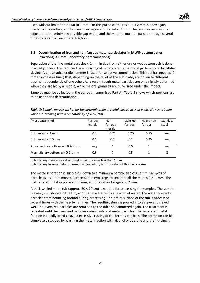
Samples must be collected in the correct manner (see Part A). Table 3 shows which portions are to be used for a determination.

Table 3: Sample masses [in kg] for the determination of metal particulates of a particle size < 1 mm while maintaining with a repeatability of 10% (rsd).

1) Hardly any stainless steel is found in particle sizes less than 1 mm 2) Hardly any ferrous metal is present in treated dry bottom ashes of this particle size

The metal separation is successful down to a minimum particle size of 0.2 mm. Samples of particle size < 1 mm must be processed in two steps to separate all the metals 0.2–1 mm. The first separation takes place at 0.5 mm, and the second stage at 0.2 mm.

A thick‐walled metal tub (approx. 30 × 20 cm) is needed for processing the samples. The sample is evenly distributed in the tub, and then covered with a few cm of water. The water prevents particles from bouncing around during processing. The entire surface of the tub is processed several times with the needle hammer. The resulting slurry is poured into a sieve and sieved wet. The oversized particles are returned to the tub and hammered again. The treatment is repeated until the oversized particles consist solely of metal particles. The separated metal fraction is rapidly dried to avoid excessive rusting of the ferrous particles. The corrosion can be completely stopped by washing the metal fraction with alcohol or acetone and then drying it.

Chemical analysis (total element contents) of MWIP bottom ashes and fl h

22

6 Chemical analysis (total element contents) of MWIP bottom ashes and fly ashes

The following describes determination methods that are applicable to crude bottom ashes and residual bottom ash processing fractions and fly ash. The descriptions focus on the preparation of samples for creating fine‐analysis samples. The actual chemical analysis methods are described in Section 11.1.

6.1 Chemical analysis (total element contents) of MWIP bottom ashes (fractions) up to 1 mm and MWIP fly ashes

Sample collection is carried out at a suitable access point using proper sampling technique (see Part A). Details of the required sample masses are given in Table 4. Figure 5 shows the determination scheme. The achievable accuracy (repeatability) is < 10% rsd, except for Au and other elements in the concentration range of < 5 mg/kg.

Fig. 5: Methods scheme for total element contents determinations from bottom ash fractions up to 1 mm particle size and fly ashes.

Sample collection

Retention sample

Comminution (e.g.. vibrating cup

mill)

Sieving 0,1 mm

Analysis sample <0,1 mm

Analysis sample metals >0,1mm

>0,1 mm

Complete digestion (Microwave)

Aqua regia digestion (open)

Analysis (ICP‐OES, ICP‐MS)


Primary sample

Sample collection

Sample preparation

Analysis

Repeated recirculation; if necessary stepwise sieving of the metal particulates (as described in text)

Backmixing

Chemical analysis (total element contents) of MWIP bottom ashes and fly ashes

23

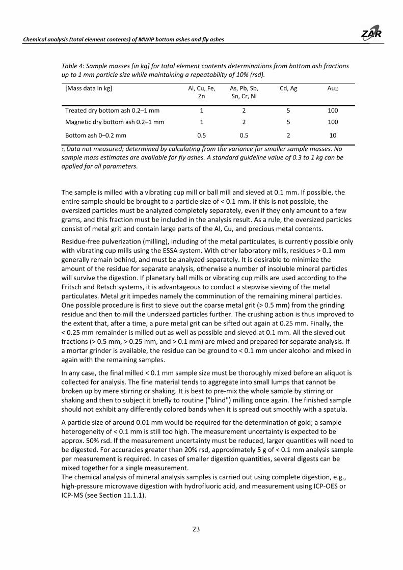
[Mass data in kg] Al, Cu, Fe, As, Pb, Sb, Cd, Ag Au1)

Zn Sn, Cr, Ni

Treated dry bottom ash 0.2–1 mm 1 2 5 100

Magnetic dry bottom ash 0.2–1 mm 1 2 5 100

Bottom ash 0–0.2 mm 0.5 0.5 2 10

Table 4: Sample masses [in kg] for total element contents determinations from bottom ash fractions up to 1 mm particle size while maintaining a repeatability of 10% (rsd).

1) Data not measured; determined by calculating from the variance for smaller sample masses. No sample mass estimates are available for fly ashes. A standard guideline value of 0.3 to 1 kg can be applied for all parameters.

The sample is milled with a vibrating cup mill or ball mill and sieved at 0.1 mm. If possible, the entire sample should be brought to a particle size of < 0.1 mm. If this is not possible, the oversized particles must be analyzed completely separately, even if they only amount to a few grams, and this fraction must be included in the analysis result. As a rule, the oversized particles consist of metal grit and contain large parts of the Al, Cu, and precious metal contents.

Residue‐free pulverization (milling), including of the metal particulates, is currently possible only with vibrating cup mills using the ESSA system. With other laboratory mills, residues > 0.1 mm generally remain behind, and must be analyzed separately. It is desirable to minimize the amount of the residue for separate analysis, otherwise a number of insoluble mineral particles will survive the digestion. If planetary ball mills or vibrating cup mills are used according to the Fritsch and Retsch systems, it is advantageous to conduct a stepwise sieving of the metal particulates. Metal grit impedes namely the comminution of the remaining mineral particles. One possible procedure is first to sieve out the coarse metal grit (> 0.5 mm) from the grinding residue and then to mill the undersized particles further. The crushing action is thus improved to the extent that, after a time, a pure metal grit can be sifted out again at 0.25 mm. Finally, the < 0.25 mm remainder is milled out as well as possible and sieved at 0.1 mm. All the sieved out fractions (> 0.5 mm, > 0.25 mm, and > 0.1 mm) are mixed and prepared for separate analysis. If a mortar grinder is available, the residue can be ground to < 0.1 mm under alcohol and mixed in again with the remaining samples.

In any case, the final milled < 0.1 mm sample size must be thoroughly mixed before an aliquot is collected for analysis. The fine material tends to aggregate into small lumps that cannot be broken up by mere stirring or shaking. It is best to pre‐mix the whole sample by stirring or shaking and then to subject it briefly to routine ("blind") milling once again. The finished sample should not exhibit any differently colored bands when it is spread out smoothly with a spatula.

A particle size of around 0.01 mm would be required for the determination of gold; a sample heterogeneity of < 0.1 mm is still too high. The measurement uncertainty is expected to be approx. 50% rsd. If the measurement uncertainty must be reduced, larger quantities will need to be digested. For accuracies greater than 20% rsd, approximately 5 g of < 0.1 mm analysis sample per measurement is required. In cases of smaller digestion quantities, several digests can be mixed together for a single measurement. The chemical analysis of mineral analysis samples is carried out using complete digestion, e.g., high‐pressure microwave digestion with hydrofluoric acid, and measurement using ICP‐OES or ICP‐MS (see Section 11.1.1).

Chemical analysis (total element contents) of MWIP bottom ashes and

24

Metallic analysis samples are dissolved using aqua regia digestion (ARD), and are likewise measured using ICP‐OES or ICP‐MS (see Section 11.1.2). The entire quantity of > 0.1 mm residue must be digested.


25

[Mass data in kg]

Al, Fe

As, Cr, Cu, Ni, Pb, Sb, Sn, Zn

Ag, Cd1)

Au2)

Treated bottom ash 0–8 mm 5 10 50 1,000

Treated dry bottom ash 0.7–5 mm 5 10 30 500

Magnetic dry bottom ash 0.7–5 mm 2 5 30 500

Crude dry bottom ash 0–5 mm 2 5 30 2,000

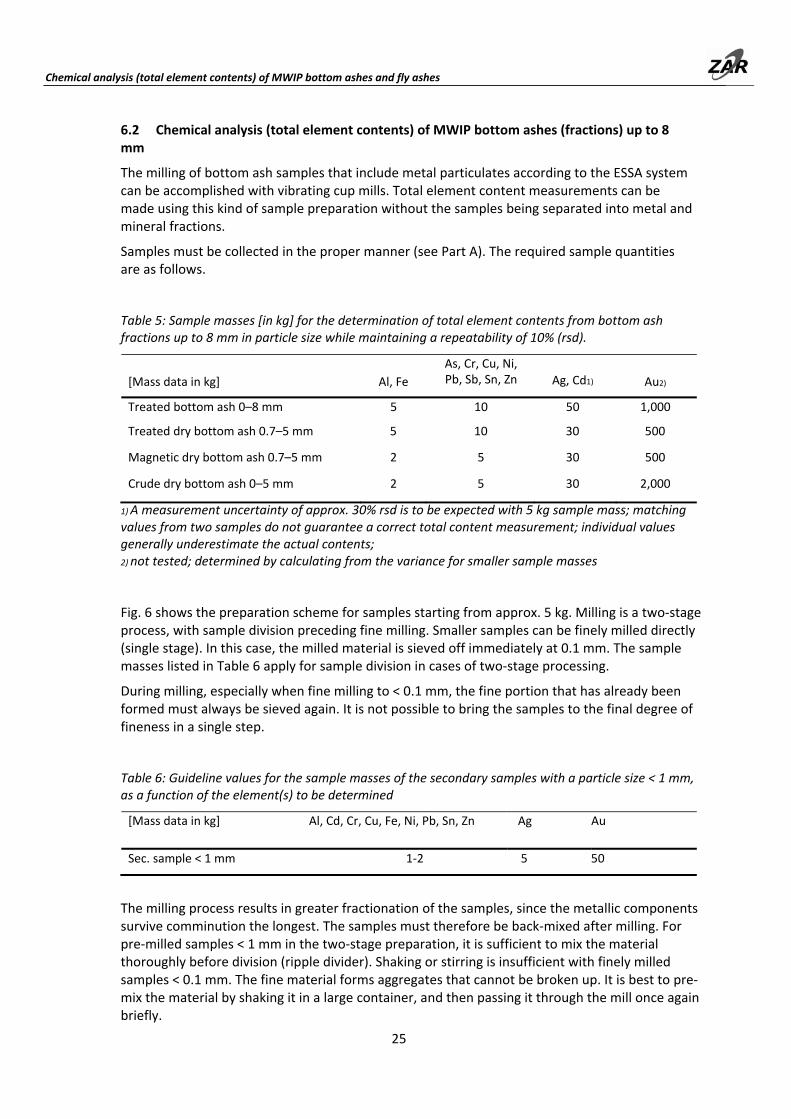
6.2 Chemical analysis (total element contents) of MWIP bottom ashes (fractions) up to 8 mm

The milling of bottom ash samples that include metal particulates according to the ESSA system can be accomplished with vibrating cup mills. Total element content measurements can be made using this kind of sample preparation without the samples being separated into metal and mineral fractions.

Samples must be collected in the proper manner (see Part A). The required sample quantities are as follows.

Table 5: Sample masses [in kg] for the determination of total element contents from bottom ash fractions up to 8 mm in particle size while maintaining a repeatability of 10% (rsd).

1) A measurement uncertainty of approx. 30% rsd is to be expected with 5 kg sample mass; matching values from two samples do not guarantee a correct total content measurement; individual values generally underestimate the actual contents; 2) not tested; determined by calculating from the variance for smaller sample masses

Fig. 6 shows the preparation scheme for samples starting from approx. 5 kg. Milling is a two‐stage process, with sample division preceding fine milling. Smaller samples can be finely milled directly (single stage). In this case, the milled material is sieved off immediately at 0.1 mm. The sample masses listed in Table 6 apply for sample division in cases of two‐stage processing.

During milling, especially when fine milling to < 0.1 mm, the fine portion that has already been formed must always be sieved again. It is not possible to bring the samples to the final degree of fineness in a single step.

Table 6: Guideline values for the sample masses of the secondary samples with a particle size < 1 mm, as a function of the element(s) to be determined

[Mass data in kg] Al, Cd, Cr, Cu, Fe, Ni, Pb, Sn, Zn Ag Au

Sec. sample < 1 mm 1‐2 5 50

The milling process results in greater fractionation of the samples, since the metallic components survive comminution the longest. The samples must therefore be back‐mixed after milling. For pre‐milled samples < 1 mm in the two‐stage preparation, it is sufficient to mix the material thoroughly before division (ripple divider). Shaking or stirring is insufficient with finely milled samples < 0.1 mm. The fine material forms aggregates that cannot be broken up. It is best to pre‐mix the material by shaking it in a large container, and then passing it through the mill once again briefly.


26

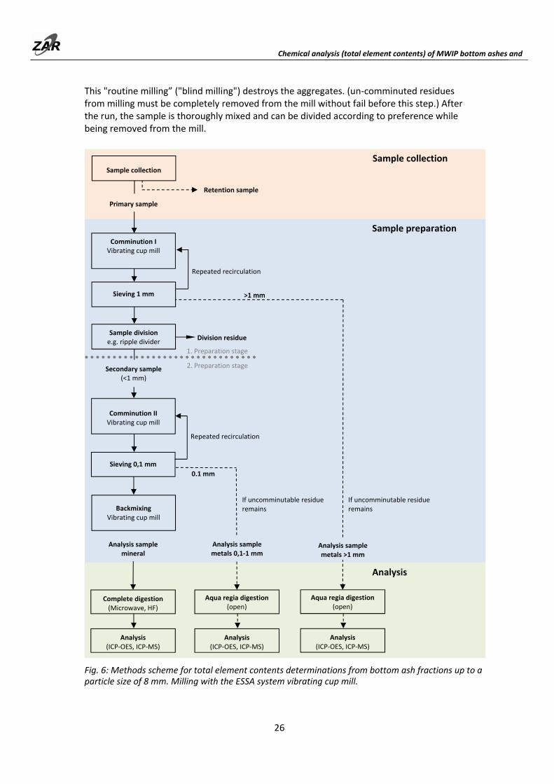
This "routine milling” ("blind milling") destroys the aggregates. (un‐comminuted residues from milling must be completely removed from the mill without fail before this step.) After the run, the sample is thoroughly mixed and can be divided according to preference while being removed from the mill.

Fig. 6: Methods scheme for total element contents determinations from bottom ash fractions up to a particle size of 8 mm. Milling with the ESSA system vibrating cup mill.

>1 mm



Analysis sample metals >1 mm

Sample preparation

Sample collection

Retention sample

Comminution II Vibrating cup mill

Sample collection

Sieving 1 mm

Comminution I Vibrating cup mill

Secondary sample (<1 mm)

0.1 mm

Analysis sample mineral

Complete digestion (Microwave, HF)




Analysis sample metals 0,1‐1 mm

Sieving 0,1 mm

Analysis

Repeated recirculation

Backmixing Vibrating cup mill

1. Preparation stage


Sample division e.g. ripple divider

Division residue


Primary sample

If uncomminutable residue remains



27

Any metallic fractions 0.1–1 mm or > 1 mm that remain will be entirely dissolved in aqua regia (ARD) and likewise measured using ICP‐OES or ICP‐MS (chapter 11.1.2).

Analysis sample particle sizes < 0.1 mm are still too coarse for the gold determination. (For weighed portions of approx. 300 mg, an ultra‐fine comminution to approx. 0.01 mm would be required for a precise determination.) Determination accuracy for samples with a particle size < 0.1 mm is around 50% rsd. Several digests can be mixed together for a single measurement to reduce the measurement uncertainty.


28

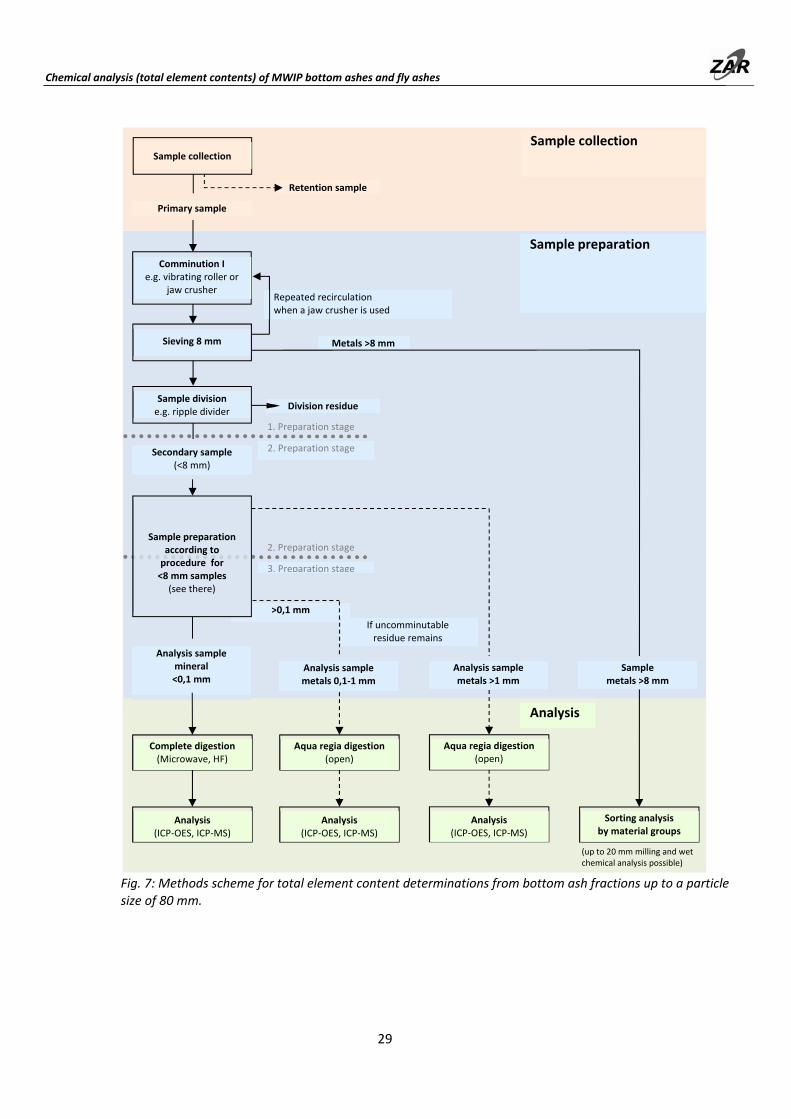
6.3 Chemical analysis (total element contents) of MWIP bottom ashes (fractions) up to 80 mm

A three‐stage sample preparation procedure is performed for samples with a particle size of up to 80 mm. The processing scheme is shown in Fig. 7. Since the primary samples are large, it is recommended to carry out the first processing step with a vibrating roller (or a mobile crusher) at the sampling site. In such cases, sample quantities of > 8 mm metal concentrate and < 8 mm residual fraction that can be easily handled are obtained on site for laboratory processing. An accuracy of about 10% rsd can be achieved if the metallic components can be milled and analyzed. If the metal composition cannot be measured directly, the uncertainty increases to 15‐20%.

Samples must be collected in the proper manner (see Part A), and with the required sample masses given in Table 7 below.

Table 7: Sample masses [in kg] for the determination of total element contents in bottom ash fractions up to 80 mm particle size while maintaining a repeatability of 10% (rsd).

As, Cr, Cu, Ni, Pb, [Mass data in kg] Al, Fe Sb, Sn, Zn Cd, Ag Au

Treated bottom ash 0–75 mm 100 300 1,000 5,000

Crude bottom ash 0–50 mm 100 300 1,0001) 5,000

1) If the contribution of NiCd batteries is to be determined at the same time: 5,000 kg for Cd

In the first preparation stage, the material is broken down to < 8 mm using a vibrating roller or jaw crusher. This comminution must be carried out in several steps as a function of the initial particle size. The largest metal pieces are either removed or sieved out from the material in each case prior to the next pass through the crusher or under the vibrating roller. (The more detailed procedure with a vibrating roller is described in Section 5.1.)

Metal fractions up to approx. 20 mm can be milled with a cooled ESSA system vibrating cup mill and then subjected to wet chemical analysis (for the procedure, see Section 9.3.2). A sorting analysis is used to sort the unmillable oversized particles into material groups, and the chemical composition is projected from typical fraction compositions (data from Table 17, page 49). If no mill is available, the entire metal fraction > 8 mm is sorted according to material groups, and the composition then projected. The procedure for sorting according to material groups is described under Section 10.

The comminuted residual fraction < 8 mm is divided. Table 8 shows the masses to be used for the second preparation stage. Further treatment of the secondary samples is analogous to the preparation of primary samples of this particle size (as described under Section 6.2). The third stage of sample preparation begins with sample division of the material comminuted to < 1 mm. The masses to be used for the tertiary samples are also given in Table 8.

Table 8: Guideline values for the sample masses of the secondary and tertiary samples as a function of the element(s) to be determined. Data in kg.

Al, Cr, Cu, Fe, Ni, [Mass data in kg] Sb, Sn, Pb, Zn Cd, Ag Au

Sec. sample < 8 mm 10 50 1,000

Tert. sample < 1 mm 1‐2 1‐2 50


29

Fig. 7: Methods scheme for total element content determinations from bottom ash fractions up to a particle size of 80 mm.

Metals >8 mm



Sample preparation

Sample collection

Retention sample

Sample collection

Sieving 8 mm

Comminution I e.g. vibrating roller or

jaw crusher


>0,1 mm

Analysis sample mineral <0,1 mm







Division residue

Repeated recirculation when a jaw crusher is used

Primary sample


Sorting analysis by material groups


Analysis

Sample metals >8 mm



Sample preparation

according to procedure for <8 mm samples

(see there)



(up to 20 mm milling and wet chemical analysis possible)


30

Cr, Cu, Ni, Sb, [Mass data in kg] Al, Fe Sn, Pb, Zn, Ag Cd Au

Crude bottom ash 0‐∞ mm 500 1,000 20,0001) 5,000

[Mass data in kg] Al, Fe Cr, Cu, Ni, Pb, Sb, Sn, Zn Cd, Ag Au

Sec. sample < 40 mm 100 200 2001) 5,000

Tert. sample < 8 mm 5 10 50 1,000

Quart. sample < 1 mm 1 1‐2 1‐2 50

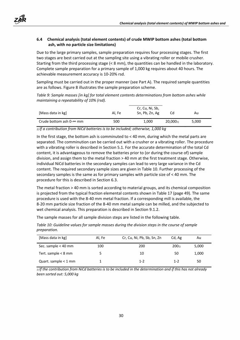
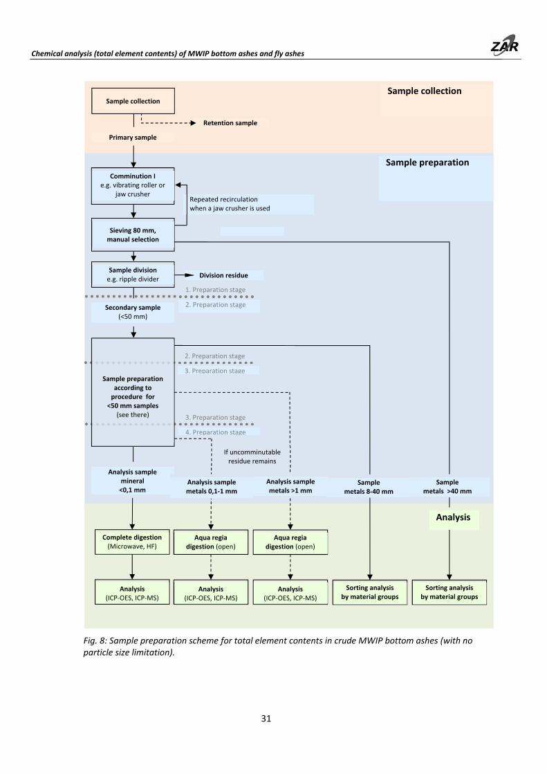
6.4 Chemical analysis (total element contents) of crude MWIP bottom ashes (total bottom ash, with no particle size limitations)

Due to the large primary samples, sample preparation requires four processing stages. The first two stages are best carried out at the sampling site using a vibrating roller or mobile crusher. Starting from the third processing stage (< 8 mm), the quantities can be handled in the laboratory. Complete sample preparation for a primary sample of 1,000 kg requires about 40 hours. The achievable measurement accuracy is 10‐20% rsd.

Sampling must be carried out in the proper manner (see Part A). The required sample quantities are as follows. Figure 8 illustrates the sample preparation scheme.

Table 9: Sample masses [in kg] for total element contents determinations from bottom ashes while maintaining a repeatability of 10% (rsd).

1) If a contribution from NiCd batteries is to be included; otherwise, 1,000 kg

In the first stage, the bottom ash is comminuted to < 40 mm, during which the metal parts are separated. The comminution can be carried out with a crusher or a vibrating roller. The procedure with a vibrating roller is described in Section 5.1. For the accurate determination of the total Cd content, it is advantageous to remove the batteries prior to (or during the course of) sample division, and assign them to the metal fraction > 40 mm at the first treatment stage. Otherwise, individual NiCd batteries in the secondary samples can lead to very large variance in the Cd content. The required secondary sample sizes are given in Table 10. Further processing of the secondary samples is the same as for primary samples with particle size of < 40 mm. The procedure for this is described in Section 6.3.

The metal fraction > 40 mm is sorted according to material groups, and its chemical composition is projected from the typical fraction elemental contents shown in Table 17 (page 49). The same procedure is used with the 8‐40 mm metal fraction. If a corresponding mill is available, the 8‐20 mm particle size fraction of the 8‐40 mm metal sample can be milled, and the subjected to wet chemical analysis. This preparation is described in Section 9.1.2.

The sample masses for all sample division steps are listed in the following table.

Table 10: Guideline values for sample masses during the division steps in the course of sample preparation.

1) If the contribution from NiCd batteries is to be included in the determination and if this has not already been sorted out: 5,000 kg


31

Fig. 8: Sample preparation scheme for total element contents in crude MWIP bottom ashes (with no particle size limitation).



Sample preparation

Sample collection

Retention sample

Sample collection

Sieving 80 mm, manual selection

Comminution I e.g. vibrating roller or

jaw crusher

Analysis sample mineral <0,1 mm







Division residue

Repeated recirculation when a jaw crusher is used

Primary sample




Sample metals >40 mm






Sample metals 8‐40 mm

Analysis


3. Preparation stage Sample preparation

according to procedure for

<50 mm samples (see there)


Determination of metallic and mineral‐bound fractions of the total element contents of MWIP bottom ashes (f i )

32

7 Determination of metal‐bound and mineral‐bound fractions of the total element contents of MWIP bottom ashes (fractions)

Most chemical elements are present in MWIP bottom ashes both in metallic form, i.e. in metal particles and pieces, as well as in oxidized form as the chemical constituents of mineral components. This type of investigation determines how the elementary fractions are distributed among the two bonding forms.

The metal particles and lumps ("metal particulates") are separated from the bottom ashes (fractions) for the determination, as described in Section 5, and then subjected separately to chemical analysis. This is how the metallic portion is quantified. The mineral‐bound fraction can be calculated as a difference based on the total content, or can be measured directly by preparing the mineral sample residue from the metal separation for fine analysis and then carrying out the analysis.

General procedure (all particle sizes) Sampling must be carried out in the proper manner (see Part A). Details of the required sample masses are listed in the following Table.

Table 11: Sample masses [in kg] for determination of the metal‐bound fractions of the total element contents from bottom ashes (fractions) while maintaining a repeatability ± 10% (rsd).

[Mass data in kg] Al, Cr, Cu, Fe, Ni, Zn Sn, Pb Ag / Au1)

Treated bottom ash 0–8 mm 10 10 50 / 1,000

Treated dry bottom ash 1–5 mm 5 10 20 / 500

Dry bottom ash 0.7–5 mm 5 10 30 / 1,000

Dry bottom ash < 0.7 mm 2 4 10 / 100

Al, Fe, Cu Cr, Ni, Pb, Zn Au

Crude bottom ash 0‐∞ mm 1,000 1,000 1,000 / 1,000

Treated bottom ash 0–75 mm crude 200 500 100 / 1,000

1) Values not measured, determined by projecting from the results from smaller sample amounts

Note: Due to its chemical properties, Au is probably always present in bottom ashes in its metallic form. The fraction that is designated as "mineral" in this determination is probably finely divided Au. In any case, the "mineral" fraction cannot be separated in the form of metal granules.

The metallic components are separated from the samples using the processing techniques described in Section 5. If the metals are separated in two or more stages, the samples can be divided after each sieving. The sample masses for division depend on the particle size as follows:

Determination of metallic and mineral‐bound fractions of the total element contents of MWIP bottom ashes (fractions)

33

Table 12: Sample masses for the division steps within the sample preparation procedure as a function of the elements to be determined. Data in kg.

[Mass data in kg] Al, Cr, Cu, Fe, Ni, Pb, Sb, Sn, Zn Ag / Au

Samples < 40 mm 300 300 / 1,000

Samples < 8 mm 10 50 / 1,000

Samples < 1 mm 1 10 / 100

The chemical compositions are determined from the metals separated from the bottom ash samples. Metals up to approx. 20 mm can be milled with a cooled vibrating cup mill in the ESSA system, and then subjected to wet chemical analysis (for the procedure, see Section 9.3.2). Metal fractions of < 5 mm can be milled in mortar grinders to < 0.25 mm under alcohol. All metals that cannot be milled are sorted according to material groups, and the chemical composition can be projected from typical fraction compositions (see Section 10).

The metal‐bound fraction of the total element contents is calculated as follows.

‐ /

/ , %

100%

Determination of scrap iron quality

34

8 Determination of scrap iron quality

The quality of scrap iron with regard to its utilization can be reliably determined only by test runs in a shredder or with test melts in a steelworks. No claim is implied in the analytical specifications listed here that the parameters obtainable from test melts or shredder test runs will be determined with the same quality. However, the parameters used in the following make it possible to define the proportions of impurities that can be influenced by the bottom ash preparation.

Samples for the determinations must be collected in the proper manner (see Part A). The sample masses required for each test can be obtained from the following table.

Table 13: Guideline values for sample masses [in kg] for the determination of scrap iron quality.

[Mass data in kg] Metal content Mass fraction of copper windings, batteries

Cu content

Fe >75 mm 200 2,000 2,000

Fe 0–75 mm 40 500 150

Fe 0–8 mm 2 ‐‐‐1) 4

Fe 0–5 mm 1 ‐‐‐1) 2

1) These objects are not present

8.1 Determination of the metal content in scrap iron (purity)

The metal content is determined by breaking down the mineral impurities by mechanical stress or releasing them from the metal. The fine mineral fraction is then sieved off.

8.1.1 Determination of the metal content in scrap iron using a vibrating roller

The scrap iron can be run over with a vibrating roller (as described for bottom ashes in Section 5.1) to release the mineral fractions from the metal. Large, solid parts, e.g. brake discs, are removed before rolling, and can be freed from adhering bottom ash by striking vigorously with a sledgehammer. For a successful release of the mineral deposits during rolling, the scrap must be spread out very thinly. No more than 50% of the support plate area should be occupied. Solid parts should be gradually discarded during processing, so that even the flat objects (cans, other metal sheets, filaments, etc.) are well covered by the roller. In the case of scrap with a particle size > 50 mm, the mineral impurities are ultimately sieved out at 8 mm. (The < 8 mm fraction still contains Fe components, but not in significant amounts.) In the case of scrap with a particle size upper limit of between 10 and 50 mm, the mineral content is sieved off at 2 mm, and for still finer materials at 1 mm. The purified metal fractions below a particle size of 5 mm should be resorted with a magnet, since in addition to iron they can contain relevant amounts of non‐ferrous metals.


35

8.1.2 Determination of the metal content in scrap iron using a vibrating cup mill, ESSA system, or equivalent type of mill in the laboratory (samples < 20 mm only)

Scrap iron up to a particle size of approximately 20 mm can be partially milled with vibrating cup mills using the ESSA system to separate out the mineral fractions. Also suitable are other types of mills that crush and beat the milled material.

The sample is subjected to brief but intensive initial milling (1–2 minutes). The coarse, clean metal pieces can then be screened out with an 8 mm sieve. The remainder is then placed back in the mill and briefly milled again. After the second milling operation, the metal is sieved at 4 mm, after a third milling cycle, the metal is finally sieved out at 2 mm. The < 2 mm residual fraction has only an insignificant iron content. Only samples with an initial particle size of less than 10 mm will also include metals at 1–2 mm. The separated metal fractions with a size < 5 mm should be re‐sorted with a magnet, since in addition to iron they can contain relevant amounts of non‐ferrous metals.

8.2 Determination of the mass fraction of copper windings, batteries, and other objects in scrap iron

The scrap iron from MWI bottom ashes contains objects that are undesirable in steel scrap, or which could be redirected to better utilization paths. These include, for example, copper windings (transformers, motors), batteries or composites of steel and non‐ferrous metals (for example, padlocks, water line valves, etc.). The proportions of these components can be determined only through sorting analyses.

8.3 Determination of the copper content of scrap iron

Precise determination of total copper content of coarse scrap iron is possible only by means of test melts in a steel mill. Only finely divided scrap up to a particle size of approx. 15 mm can be milled to powder and analyzed by wet chemical methods. (For milling and analysis analogous to the procedure for non‐ferrous metal products, see Section 9.3.)

Benchmark copper values for coarse scrap can be determined by separately determining the contributions of copper‐carrying components (windings, etc.), mineral impurities, and the iron metal itself. The procedure is as follows.

Contribution from the copper‐carrying components that can be sorted out The mass fractions of the copper‐carrying components (windings, steel‐non‐ferrous metal composites) are determined through a sorting analysis (see Section 8.2). The contributions of these copper‐carrying components to the total copper content are calculated as approximations. The mass fraction of the windings is multiplied by 0.18, and that of the non‐ferrous metal composites by 0.3.

Contribution from mineral impurities The copper in mineral impurities contributes significantly to the total copper content of scrap iron. The bottom ash deposits contain both oxidized copper in the mineral fraction as well as non‐ferrous metal particles. The mass fraction of Fe metal and impurities must first be determined in order to determine the contribution of the bottom ash deposits to the total copper content of the scrap (see Section 8.1). Of the separated impurities, 5 kg is milled as for bottom ash samples, and this is then analyzed by wet chemical methods (see Section 6.2).


36

Contribution of ferrous metals The ferrous metal pieces themselves also contain a large portion of the total copper content in scrap iron. ("Stains" or drops of non‐ferrous metals are melted onto many steel parts. An accurate determination is not possible without melting a large quantity of iron metal.) However, benchmark values can be measured by boring samples from many ferrous metal pieces and analyzing them as a mixture by wet chemical techniques. For such an analysis, at least 30 parts are randomly selected from the scrap, and are drilled with a 3 mm drill and the borings are collected. Large, flat parts are drilled several times, so that approximately one drill hole has been made per square decimeter. Thick objects that cannot be drilled through are then drilled in this way more frequently, so that the total drilling depth corresponds to the thickness of the object. (In such cases, only the borings from the surface are included in the sample, and that from the other holes is discarded.) The borings in the sample are then digested in aqua regia, and measurements are made using ICP‐OES or ICP‐MS (see Section 11.1.2)

Determination of the quality in non‐ferrous products

37

9 Determination of the quality of non‐ferrous products

As a rule, crude non‐ferrous scrap is not characterized until it is undergoing processing, during which the user determines the yields of aluminum and non‐ferrous metals in each batch (for billing purposes). Also, it is usually the user who performs the analysis in the case of aluminum and non‐ferrous metal scrap. At smelting plants, such materials are usually melt‐blended into the sample to determine the parameters relevant to billing. Non‐ferrous products can be tested for their mass fractions of aluminum and heavy non‐ferrous metals and their chemical compositions using the analytical methods described below.

9.1 Determination of the metal content in non‐ferrous products

The metal content of non‐ferrous products is determined by breaking down and sieving off the mineral particles and caking, and washing off any adhering bottom ash fines. For fine‐grained, heavy, non‐ferrous products, the metal content can also be determined as the metal yield from a melt with borax flux (see 9.3.1). The prerequisite for this is the formation of a low‐viscosity borax bottom ash that enables good separation between metals and bottom ash.

Table 14: Sample masses [in kg] for determination of the metal content of non‐ferrous products while maintaining a repeatability of 10% (rsd).

[Mass data in kg]

Non‐ferrous 8–75 mm (crude) 5

Non‐ferrous 0–8 mm (crude) 1

Non‐ferrous, light, 3–5 mm, from dry bottom ash 0.5


Non‐ferrous, light, 0.2–1 mm, from dry bottom ash 0.05

Non‐ferrous, heavy, 3–5 mm, from dry bottom ash 2


Non‐ferrous, heavy, 0.2–1 mm, from dry bottom ash 0.1

Two options for separating mineral constituents from metal are described below. The choice of variant is left up to the user. Treatment with a vibrating roller can be carried out directly at the sampling site and is suitable when bottom ash samples are also processed on site in the course of a larger study.

9.1.1 Determination of the metal content in non‐ferrous products using a vibrating roller

The general procedure and equipment required for the separation of metal and mineral substances using a vibrating roller are described in Section 5.1. The sample is weighed before processing. The mass fraction of the clean metals obtained therefrom is given as a metal content.

To achieve a good separation between metals and minerals, the sample material must be distributed thinly across the support plate. The particles should not cover more than one‐third of the area. In addition, processing with the roller must be performed in several steps.

The largest metals are sieved out after each rolling operation. The under‐sized particles are redistributed across the plate and rolled over once again. In this way, the metal is obtained from


38

the sample step‐by‐step, and the mineral residue remains behind as under‐sized particles. The first sieving takes place with a sieve mesh size of approximately half the maximum particle diameter. The mesh size should be reduced no more than by half from one step to the next. For a coarse, non‐ferrous starting material at > 10 mm, the final product is sieved off at 2 mm, while finer starting material is sieved off at 1 mm.

Despite intensive processing, individual mineral particles can remain behind in the separated metals, particularly flat pieces such as glass and ceramic flakes. These foreign objects must be discarded from the metal before it is weighed. With large quantities of fine‐grained metals, the proportion of residual mineral particles can be determined using partial samples. The partial samples must be obtained using ripple dividers. The size of the partial samples is selected in such a way that more than 30 mineral particles can be picked out for analysis during the discard.

Non‐ferrous products with wet or dried finely divided adhesions must be washed before or after rolling. A concrete mixer can be used for this purpose. The sample material is admixed with a 10% citric acid solution and run in the mixer for about 20 minutes. The material is subsequently washed out on a sieve. A 2 mm sieve should be used for starting material > 10 mm, while for finer starting materials a 1 mm sieve is employed.

9.1.2 Determination of the metal content in non‐ferrous products using a vibrating cup mill, ESSA system (or equivalent type of mill) in the laboratory

The determination can be carried out using an ESSA system vibrating cup mill, or another type of mill that crushes and beats the milled material.

The separation of clean metals from the samples takes place by stepwise milling and sieving. The material is milled for only a short time so that mineral pieces or particles are broken down, and any caking flakes off from the metal parts. The milling takes about 1–2 minutes in the LM 5 mill. After each milling run, the material is sieved to separate out the metal parts that have already been cleaned. After the first mill run, a sieve with a mesh size of approx. half the maximum particle diameter is used (e.g., 10 mm for an initial particle size of up to 20 mm). The sieve mesh size is reduced by approximately half following each additional grinding operation. Non‐ferrous products with an initial (maximum‐size) particle size greater than 10 mm are milled and sieved down to 1 mm, while finer starting materials are sieved down to 0.25 mm.

Milling in the LM 5 mill applies considerable abrasion to the non‐ferrous metal particles. This means that a portion of the metal (up to 10%) is ultimately to be found in the mineral material fraction in the form of fine grit. The metallic aluminum portion of the mineral material fraction can be measured by the hydrogen method (see Section 11.2). In this way, the slippage can thus be determined at least for the aluminum, and the result can thus be corrected.

The metal content is calculated as follows:

, / , , ‐ ,mineral /


39

9.1.3 Determination of the metal content in non‐ferrous products of < 1 mm using a needle hammer

In the particle size range below 1 mm, the metal is separated from minerals by processing with the needle hammer. The needle hammer procedure is described in Section 5.3 for fine bottom ash fractions. The operative principles are the same for non‐ferrous products. The sample is hammered until no mineral particles remain.

When working with a needle hammer, some slippage of metals into the fine mineral fraction (sludge) will occur. To correct the result for this slippage, a sample is removed from the sludge immediately after sieving, and the proportion of metallic aluminum contained therein is determined (for the determination method, see Section 11.2). The remainder of the sludge is dried to determine the water content. The metal content is calculated using the formula given in Section 9.1.2, whereby the total quantity of the sludge is used as follows.

, ∑ ‐ . , ,

,

The aluminum metal content of the sludge must likewise be used as a dry‐related value in the formula in Section 9.1.2.

9.2 Determination of the extraneous matter in heavy and light non‐ferrous products, and of the heavy and light non‐ferrous content in crude non‐ferrous products

In this case, metal particles of one type present in the respective other product, i.e., heavy non‐ferrous metal particles in light non‐ferrous products and light non‐ferrous metal particles in heavy non‐ferrous products, are referred to as extraneous constituents.

To determine the proportion of light components in heavy fractions and vice versa, the samples are sorted by density using the float‐sink method. A ferro‐silicon dense medium or a sodium polytungstate solution is used as the separation medium. The density separation in the liquid separation medium ensures that the separation occurs exclusively according to particle density; particle shape and size do not matter. This determination method can also be used to measure the proportions of heavy and light non‐ferrous metals in crude non‐ferrous recyclable fractions.

The sample masses required for the determination depend strongly on the mass fraction of the extraneous constituents to be determined. The lower the content, the greater the sample mass needed. Guideline values for all sample masses are given in the following table. Since the particles to be detected can be identified and counted, it is also possible to determine the required sample masses directly from the material according to the “100 particles rule”. The samples should be large enough to contain approx. 100 of the particles sought. The samples must be collected in the proper manner (see part A), and optimally be divided into the target masses using ripple dividers.


40

Table 15: Guideline values for sample masses [in kg] for determining the extraneous constituents in density‐sorted non‐ferrous recyclable fractions, and for determining the heavy and light content in non‐ferrous metal mixed fractions. Values in kg for maintaining a repeatability of 10% (rsd).

[Mass data in kg]

Non‐ferrous, crude, 8–75 mm 10

Non‐ferrous, crude, 0–8 mm 2

Non‐ferrous, light, 3–5 mm, from dry bottom ash 2


Non‐ferrous, light, 0.2–1 mm, from dry bottom ash 0.1



Non‐ferrous, heavy, 0.2–1 mm, from dry bottom ash 0.1

The ferro‐silicon dense medium is a slurry with a slightly thixotropic character, i.e. it solidifies when it is not being moved. Small particles of less than approx. 5 mm in size do not rise or sink by themselves in the undisturbed dense medium, but remain “stuck”. If the dense medium is moved gently, a sorting of samples from a particle size of 1 mm is readily possible. The sodium polytungstate solution does not have thixotropic properties, and is thus better suited for finely divided samples.

Density‐based separation in a ferro‐silicon dense medium Ferro‐silicon dense media is used in large‐scale float‐sink systems for the separation of mixed scrap. This dense liquid is a slurry of ferro‐silicon powder (FeSi) and montmorillonite (clay mineral) in water. The montmorillonite is an important component because it stabilizes the suspension, which means that densities of up to approx. ca. 3 g/cm3

can be achieved.

FeSi powder and montmorillonite are not readily available commercial chemicals. The material is best obtained from a scrap processor. The dense medium is prepared from an approximately 10% montmorillonite slurry by blending in FeSi powder until the required density of approximately 2.8 g/cm3 is achieved. (Note: It is not absolutely necessary to measure the density; it is sufficient to confirm that a piece of aluminum can float in it.) The suspension should be stable enough that the FeSi (and thus the floating aluminum piece) does not sink appreciably within the space of one minute. If necessary, add more montmorillonite.

The float‐sink separation is best carried out in a square tub. The sample is weighed before being distributed into the dense medium. The dense fluid loading should maximally be high enough that the floating aluminum layer is no more than 3 times thicker than the maximum particle size (i.e., not more than 1.5 cm for a metal fraction of 1‐5 mm). The mixture is first stirred, then moved only indirectly by swaying the pan gently back and forth. The dense medium must always remain in motion, so that a complete separation can be achieved. Finally, the liquid is poured into a sieve along with all of the floating aluminum. If necessary, the dense medium must be poured back again to extract all the aluminum.


41

The aluminum is washed in the sieve and dried, and the sludge fraction from the tray is also washed and dried.

(Note: Wire coils or hollow particles (e.g., the brass sleeves of ballpoint pens) made of heavy non‐ferrous material often enter the floating fraction because they contain air bubbles, but that fraction is usually insignificant and the sharpness of the separation will nonetheless exceed 99%.)

Density‐based separation in a sodium polytungstate solution Sodium polytungstate is expensive (about 300 CHF/kg, corresponding to approx. CHF 900/L separation medium), and its use as a separating medium is thus only useful for small, finely divided samples. A solution with a density of 3 g/cm3

is prepared by mixing sodium polytungstate

and water in a ratio of 6:1 (85% solution). The float‐sink separation can easily be carried out in crystallizing dishes. The sample is blended into the liquid, and the floating fraction together with the solution is poured into a sieve. The floating and sinking fractions are then washed with water and dried.

(Note: The wash water can be evaporated to recover the sodium polytungstate. Although the polytungstate solution takes on an intense blue color when it comes in contact with aluminum, this coloration has no effect on the usability of the solution. The color gradually disappears immediately under the influence of oxygen. The solution can be decolored with H2O2 .)

9.3 Chemical analysis (total element content) of non‐ferrous products

In the metallurgical field, most metal samples are melted to produce homogeneous samples for analysis. However, it is not easy to cull out the metal content of a non‐ferrous metal sample in a completely homogeneous melt bath. Flux must be added during melting to dissolve the oxide layers on the metal particles, and facilitate the incorporation of all the other mineral constituents into a liquid bottom ash. The following basic requirements are applicable to melt samples for analysis:

– the metal content of the sample must completely coalesce in a bath; – the metal and flux, together with the impurities, must lend themselves to complete

separation; – the molten bath is permitted to have only one liquid metal phase; – it must be ensured that all analytes are dissolved and quantitatively culled out in the

liquid metal phase, otherwise the flux bottom ash must also be included in the analysis;

– the analysis samples must be homogeneous, and gradients within the sample bodies (as a result of segregation) must be able to be excluded.

In the following, only one melting method is described for finely divided, heavy, non‐ferrous products weighing up to 600 g. At present, only for this method has it been confirmed in detailed experiments that the metal fraction is quantitatively culled out in the molten bath and that homogeneous analysis samples can be taken. However, it should also be possible to use melts with a borax flux for coarse‐grained, heavy, non‐ferrous products and larger sample weights. Light, non‐ferrous products can be melted in the presence of salts, as is common in secondary metallurgy. However, complete separation is difficult due to the low density difference between the liquid metal and salt bottom ash. No confirmed method is yet available. For crude non‐ferrous products (heavy/light mixtures), a melt with a high metal yield is not possible due to the limited mutual solubility of the various metals and the differing requirements for fluxes.


42

As an alternative to using a melt, non‐ferrous products can be comminuted to an initial particle size of about 20 mm. Comminution is possible with a cooled version of the ESSA system LM 5 vibrating cup mill. The chemical nature of the samples remains unchanged during comminution. It is thus also possible to measure parameters for which error‐free determinations cannot be made from melts, e.g., the aluminum content of non‐ferrous products, since the aluminum partially bottom ashes when melted.

Chemical analysis can provide only indirect characterizations of coarse‐grained and lumpy non‐ferrous metal samples that can neither be milled nor melted. For this purpose, the samples are fractionated into material groups and the chemical composition is calculated from the typical element content for those fractions (see Section 10).

The minimum sample masses for the chemical analyses of non‐ferrous products depend strongly on which elements are to be determined. A compilation of sample mass data is provided in Table 16.

Table 16: Guidelines for sample masses [in kg] for element total content determinations in non‐ferrous products while maintaining a repeatability of 10% (rsd).

[Mass data in kg] Al, Cu, Zn, Pb Fe, Ni, Sn Cr, Sb Ag, Cd Au

Non‐ferrous (crude) 0.7–5 2 5 10 100 3001)

Non‐ferrous (crude) 0–8 mm 5 10 10 50 5001)

Non‐ferrous (crude) 8–75 mm 50 500 500 1,000 ‐‐‐

Al, Cr, Cu, Fe, Ni, Zn As, Sn, Pb, Ag, Sb Cd, Au

Non‐ferrous, light 0.2–1 mm 1 1.5 5

Non‐ferrous, light, 1–3 mm 1.5 3 10

Non‐ferrous, light, 3–5 mm 2 5 501)

As, Cr, Fe, Ni,Al, Cu, Pb, Zn Sb, Sn Ag / Cd Au

Non‐ferrous, heavy 0.2‐1 mm 0.25 0.5 0.5 2

Non‐ferrous, heavy 1‐3 mm 0.5 3 3 / 15 301)

Non‐ferrous, heavy 3‐5 mm 1 5 10 / 20 1001)

Non‐ferrous, heavy 1‐5 mm 1 5 5 / 20 1001)

Non‐ferrous, heavy 5‐10 mm 2.5 10 30 5001)

1) Not tested; calculated from the results from smaller sample sizes


43

9.3.1 Chemical analysis (total element content) of non‐ferrous products up to 5 mm in a melt

Heavy non‐ferrous products can be remelted with high metal yields with the addition of borax as a flux. The metal melt culls out the Cu and precious metals in their entirety. More than 98% of the Pb, Sn, Ni, As and Sb can also be carried over into the molten metal bath, and more than 95% of the Zn. The melt is homogeneous with respect to these elements. Representative samples can be drawn from the molten bath with the aid of suction samplers. However, test pieces in the form of "lollipops" are not always homogeneous throughout their cross‐sections. If the lollipops are measured using a spark spectrometer (F‐OES), measurements must be made at several depths to check homogeneity. When preparing borings, the lollipops must be drilled at several points and the shavings must be mixed well. A closely matrix‐adjusted calibration is necessary when F‐OES is used to measure some of the trace components, such as Au. Melts are not suitable for determinations of Al, Cr and Fe, and metallic Al bottom ashes in the melt. Conversely, the melt will absorb Fe depending on the residence time, presumably through corrosion of the crucible material. Cr is unevenly distributed in the test pieces, so that substantial variance will be observed in F‐OES analyses, as well as in wet chemical analyses.

The melt is prepared in a clay‐graphite crucible in an induction furnace. A powerful air extraction system is absolutely required when using a smelting device, since zinc burns under certain circumstances and large amounts of ZnO smoke are generated. The sample material is weighed and placed in the crucible together with anhydrous borax as a powder. Borax in the amount of about 10% of the sample weight is added for metal fractions of high purity. The borax should be distributed as evenly as possible in the crucible filling, and the crucible filling should be packed as densely as possible. The higher the proportion of mineral impurities, the more borax must be added. The borax bottom ash must be free‐flowing when heated so that all the metal can flow into a melt bath. It is also possible to melt a portion of the samples first and then to re‐charge the remainder into the liquid preparation. The temperature must be controlled such that the melt is kept as close as possible to just below its boiling point. (The boiling point of the mixture is in the range of the melting point of pure copper, and a temperature that is too low can lead to segregation of the lead.) Boiling heavy non‐ferrous melts produce bright shining zinc fires with strong smoke emission in which appreciable amounts of zinc may be lost. The frequency of the induction heating should be chosen in such a way that the molten bath is vigorously mixed. Without intensive mixing, a second liquid phase of lead may adhere to the crucible base. After melting is complete, the melt is maintained at a temperature of 1,000–1,100°C for a few minutes, so that all the constituents, especially the Pb, will dissolve in the Cu‐Zn liquid phase. The borax must be supplemented if the bottom ash is not of sufficiently low viscosity to ensure that all of the metal will coalesce well.

The melt is then sampled, e.g., with a suction sampler, or a test piece mold is filled when the melt is poured off. After sampling, the remaining melt is poured off. The cold metal block must be freed from the borax bottom ash with strong hammering because the pure metal must be weighed. If metal drops (globules) are included in the decanted borax bottom ash, this bottom ash must be broken up to release those globules. Likewise, all the metal remaining in the crucible must be recovered for weighing. Everything that is metal (block, test pieces, and metal from the borax bottom ash and crucible) is weighed. The melt yield is calculated from the mass as follows.

%

100%


44

For wet chemical analysis, borings are drilled out of the test pieces and are digested (see Section 11.1.2). For F‐OES measurements, the test pieces are ground flat, or milled or machined flat.

The total elemental contents of the original samples are calculated from the analysis results of the molten metal as follows.

/ / %

100 %


45

9.3.2 Chemical analysis (total element contents) of non‐ferrous recyclable material fractions up to a particle size of 20 mm through comminution

This type of sample preparation can be carried out using a cooled, ESSA system LM 5 vibrating disk mill. Samples that are larger than one mill filling are comminuted in two stages, and are divided before the second milling stage. Figure 9 shows a schematic of the two‐stage processing. Smaller samples are comminuted to < 0.1 mm in a single step. In this case, the pre‐comminution to < 1 mm and the sample division are omitted.

The samples can neither be milled to < 1 mm during pre‐comminution nor finely comminuted in a single step because the fines fraction tends to clump up. The samples are therefore sieved repeatedly to separate out the fines fraction already formed. Depending on the initial material and the progress of comminution, milling times of two to ten minutes between sieving steps are possible. The samples must be re‐mixed after fine milling before an aliquot is taken for analysis. This mixing involves the entire finely ground sample being shaken vigorously in a sufficiently large container.

The analytical weighings are dissolved by aqua regia digestions, and measurements are made using ICP‐OES or ICP‐MS (see Section 11.1.2). Any milling residues are entirely digested and analyzed separately.


46

Fig. 9: Diagram showing determinations of total element contents in non‐ferrous products of < 20 mm using a two‐stage comminution (ESSA system vibrating cup mill, cooled)

>1 mm



Analysis sample milling residue >1 mm

Sample preparation

Sample collection

Retention sample

Comminution II vibrating cup mill

Sample collection

Sieving 1 mm

Comminution I Vibration cup mill


0,1 mm

Analysis sample <0,1 mm





Analysis sample milling residue 0,1‐1 mm

Sieving 0.1 mm

Analysis


Backmixing




Division


Primary sample



Sorting analysis of metal samples by material or product group

47

10 Sorting analysis of metal samples by material or product group

Mixed metals can be separated from the bottom ash during metal content determination and can be fractionated according to material groups through magnetic and density sorting. Figure 10 summarizes the options for fractionation.

Fig. 10: Options for fractionating mixed metal samples derived from MWIP bottom ashes

Segregation and fractionation of ferrous metals In the first step, the strongly ferromagnetic ferrous metal is removed from the mixture using a magnet. Fe metal "jumps" to the magnet, and cannot be shaken off. By contrast, the highly alloyed, rust‐free grades (stainless steel) can be lifted out only by direct contact with the magnet, and will fall off when the magnet is shaken. Cu windings (transformers, electric motors, other coils) and batteries also fall into the strongly magnetic fraction. If necessary, these objects can be manually picked out from the ferrous metal.


48

Differentiation of battery types If necessary, battery types can be distinguished according to their internal structure. If a battery is sawed open in the lower third of its structure, carbon black will become visible in instances of zinc‐charcoal cells; in the case of alkaline‐manganese cells, the discharge mandrel is made of brass. In the case of rechargeable cells, the electrodes are rolled up inside in a spiral. Nickel‐metal hydride cells can be distinguished from nickel‐cadmium cells by performing a qualitative test for Cd. For this purpose, a few granules or dust from the battery contents are applied to a filter paper strip moistened with 10% acetic acid. The acid should take about 1 minute to act. The strip is then exposed to hydrogen sulfide. The simplest way to do this is to place a small amount of FeS in a test‐tube with some dilute hydrochloric acid, and then clamp the strip in the test tube with a cork. The filter paper turns yellow around the sample granules if they contain Cd. (Note: Lithium ion batteries burn, and are not found in MWIP combustion residues.)

Density separation for non‐ferrous metals Density separation is carried out by the float‐sink procedure in a ferro‐silicon dense medium for samples starting from a particle size of 1 mm, or in sodium polytungstate solution for finer particles. This method is described in Section 9.2.

The light metal fraction also includes most of the mineral particles (glass, ceramics, etc.). These foreign components must be discarded before the light metal fraction is weighed.

Further fractionation of heavy non‐ferrous metal samples In addition to non‐ferrous metals, zinc and lead, this fraction also contains the weakly or non‐magnetic grades of steel, primarily stainless steel. Steel parts can be easily recognized because they are still in the form of the original articles. Frequently encountered examples include sheet metal strips and wires, springs, razor blades, and injection needles. In contrast, the non‐ferrous metals are usually particulates, because they melt into droplets and nuggets. The actual heavy non‐ferrous metals can be further divided into material groups according to their color. All copper‐colored particles are combined in a “copper” fraction, and yellowish‐gold particles make up “brass/bronze” fraction. The zinc fraction is light gray with a slightly bluish tinge, and the lead fraction is dark gray and additionally characterized by its easy deformability and high density.

The data in Table 17 can be used in the calculations when the results of a sorting analysis are to be used to estimate the chemical composition of the sorted sample.


49

Table 17: Typical values for fractions to be used in calculations of the chemical composition of sorted metal samples. (Source: Skutan and Rechberger, 2007)

Ferrous metals

Windings

Alkaline batteries

Zinc‐carbon batteries

Ni/metal hydride batteries

NiCd batteries

Fe 92% Fe 70% Cu 18%

Mn 28% Fe 19% Zn 18% Cu 1.5%

Zn 20% Mn 17% Fe 16%

Ni 41% Fe 27% Co 4%

Fe 39% Ni 21% Cd 18%

Aluminum

Copper

Brass/ bronze

Zinc

Lead

Stainless steel

Al 81% Cu 96% Cu 60% Zn 86% Pb 90% Fe 66% Zn 1% Cu 0.6%

Ni 0.5% Zn 36% Pb 1.5%

Pb 1.8% Cu 0.7%

Sn 2.5% Sb 1%

Ce 17% Ni 10%

Ni 0.8% Ni 0.4% Sn 0.4% Sb 0.3%

Digestion and analytical methods for ready‐prepared analytical samples

50

11 Digestion and analytical methods for ready‐prepared analytical samples

11.1 Determination of total element contents in analysis samples

Standardized wet chemical methods are available for the determination of total element contents. For these reasons, the analytical methods are treated here only very briefly. The accuracy of the determinations can be verified with certified reference materials (for example, fly ash as materials of similar matrix composition).

XRF analysis systematically underestimate total element contents when the analytes are present in metal particles > 5 µm. For example, only 50% of metallic copper was detected in samples with a particle size of < 63 µm. Systematically low findings were also confirmed for the main components in powders of aluminum, brass, zinc, and lead (Bachema, 2012). Adequate comminution that also includes the metallic components can be achieved only through wet milling (agitator mills). Recovery is around 80% in the 10‐20 µm particle size range, which is achievable through wet milling in a mortar mill. Neither of the two wet milling techniques has currently been sufficiently tested in the preparation of samples intended for XRF measurements to ensure reliable recovery.

11.1.1 Total element content determinations for mineral materials using complete digestion and measurements by ICP‐OES or ICP‐MS

For total content determinations, the sample matrix must be completely decomposed through total digestion. To achieve this, acid mixtures containing hydrofluoric acid are used. This is usually accomplished using microwave‐assisted pressure digestions in accordance with SN EN 13656:2002. Other methods can also be used, e.g., high‐pressure digestion. The quality of the digestion process is determined in each case using certified reference materials, e.g., those listed in the BCR 176R Standard. Measurement of the constituent elements in the digestion is carried out using ICP‐OES in accordance with SN EN ISO 11885, or using ICP‐MS in accordance with SN EN ISO 17294‐2.

The sample weights (test quantities) used in microwave digestion are around 500 mg. Within the limits of determination, weighings of this size should suffice in most cases for analyzing these constituent elements. Only the Au content of the bottom ashes (fractions) is close to the limit of determination for the analytical system (roughly 10 mg/kg for ICP‐OES, and 0.1 mg/kg ICP‐MS). Moreover, with regard to reproducibility (i.e., homogeneity of fine analysis samples of < 100 µm), a starting weight of 500 mg is sufficient for most parameters. A repeatability of a few % rsd can be achieved for the elements Al, Fe, Cr, Ni, Cu, Zn, Sn, Pb. Cd and Ag can be determined with around 10% rsd, and only Au cannot determined accurately. The test quantity required is roughly 10 g, which means that the solutions from approximately 20 digestions must be mixed together for accurate determinations. (Note: All analyses can of course also be measured individually. The analytical result is then an average value weighted by the sample quantities, but under no circumstances can “outliers” be excluded from the calculation of the mean value, even if the variance is large.)

Note: What is known as a “fire assay” is used in precious metal analysis, which allows for larger amounts of sample, but this has not yet been tested for MWI bottom ashes. The process is certainly suitable, but ‐ as for every material ‐ the proper formulation of lead oxide, reducing agent and flux must first be found.


51

11.1.2 Total element content determinations for metallic samples by digestion in aqua regia, and measurement using ICP‐OES or ICP‐MS

Metallic samples are dissolved in aqua regia, a digestion method that is covered in SN ISO 11466. The samples are heated to reflux, with adsorption tubes filled with dilute nitric acid 0.5 M to prevent the loss of Hg and metal hydrides. The element concentration measurements from the digest are carried out using ICP‐OES as per SN EN ISO 11885, or ICP‐MS as per SN EN ISO 17294‐2.

The digestions are carried out with weighings of about 3 g. If the samples are rich in base metals, large amounts of hydrogen will be produced during the dissolution. The acid must be added in portions so that the gas formation does not take place too violently. The absorption vessel must be placed in line immediately after the first addition of acid to capture the gaseous metal hydrides. The hydrochloric acid is added first, and the nitric acid is not added until the reaction has calmed down. The nitric acid must also be added one portion at a time, and the first mL of the nitric acid will elicit substantial foaming.

The digestions only rarely produce clear solutions, since most metal samples contain insoluble silicate‐type impurities, and additionally, among other things, the Si that is contained in light metal alloys will generate

an SiO2 precipitate. The silicate sludge is not relevant to the analysis, although when filtering the digestion solutions, it is necessary to check whether crystalline or flaky precipitates are present. (Note: Completed digestions must also be checked for crystalline concentration precipitates before measurements are made, because such crystals may form hours or even days later.) Such precipitates may be salts or oxides of Ag, Sn, or Pb, and can be dissolved in dilute hot hydrochloric acid (PbCl2), cold concentrated hydrochloric acid (cassiterite, SnO2), or nitric acid (AgCl). Separately dissolved precipitates should be measured separately to avoid re‐precipitation that can occur when admixed into the digest solution. In cases of concentration precipitates, it is advisable to repeat the digestion with a smaller initial weight to determine once again the constituents that were at the solubility limits.

When dissolving granular metal samples (for the determination of the metal‐bound element content, see Section 7), Pb particles often remain behind in the residue. Pb becomes passivated in the aqua regia, and dissolves better in hydrochloric acid.

11.2 Determination of metallic aluminum through hydrogen evolution

Metallic aluminum decomposes in strong alkali to form hydrogen gas. The gas that is generated can be measured volumetrically, and from this the quantity of metallic aluminum present can be calculated. The initial weights required for the determination are given in Table 18.

Table 18: Guideline values for weighings for determining metallic aluminum in bottom ash samples.

Type of material Weighing

Milled samples < 0.1 mm from 100 mg (Selected according to gas formation)

Treated dry bottom ash 0.2‐1 mm 5 g

Magnetic dry bottom ash 0.2‐1 mm 10 g

Dry bottom ash 0‐0.2 mm 5 g


52

In principle, the determination can also be used for samples with a particle size greater than 1 mm. The sample quantities to be used, and consequentlstay the resulting gas quantities, are however (1) high, and (2) particulate samples quite readily self‐segregate, which means that the weighings can hardly be considered to be representative.

The measurement is based on volumetric carbonate determination according to Scheibler (cf. DIN ISO 10693: 1997). The design of the Scheibler apparatus is shown in Fig. 11. To minimize H2 losses due to diffusion, a thin Teflon hose should be used between the reaction vessel and the apparatus instead of a silicone rubber hose.

The sample is weighed into the reaction vessel, and a beaker is inserted into the center of the reaction vessel, and this is filled with a 10% sodium hydroxide solution using a pipette. The reaction vessel is connected to the apparatus, and the water column in the measuring tube is set to zero. To accomplish this, the upper stopcock on the measuring tube and the pinch cock on the line to the compensating vessel are opened and the compensating vessel is raised until the water level is set to exactly zero. The upper stopcock is then closed. The reaction vessel is then tilted and swirled until the alkali solution and the sample are mixed. Depending on the sample, the gas formation takes minutes to hours. Milled samples react very quickly. Crude samples do not begin reacting until after a few minutes have passed and the gas formation takes a long time. The level is read off once the volume has stopped increasing. For the reading, the pinch cock to the compensating vessel must be opened and sufficient water must be discharged from the apparatus for the water levels on the left and right of the U‐tube to be the same.

Fig. 11: Scheibler apparatus for measuring the gas formation in chemical reactions. (Image source: Schlichting, et al., 1995, modified)

The content of metallic aluminum in the initial mass of test portion can be calculated using the following formula:

/ 0,21621 ° 273,15

Glossar

53

Glossary

Analytical sample, sample in the state of having been prepared for analysis, from which the portions are taken for the actual analysis step (e.g., digestion, or direct measurement using XRF)

Analysis portion, amount of the analytical sample (analysis weighing) to be used in the actual analysis procedure (e.g., digestion or XRF measurement)

Increment, subset of the quantity to be characterized (entire quantity), which by itself does not represent the entire quantity; only an aggregate of all of the increments from a sampling results in a representative sample

Primary sample, sample that is taken directly from the bulk material (usually as a mixture of many increments)

Sample, a partial quantity from the quantity of material (bulk material) to be characterized, which by itself represents the properties of the bulk material

rsd, relative standard deviation or coefficient of variation; calculated as a standard deviation in % of the mean value

Secondary sample, partial sample prepared by sample division from the primary sample

Systematic errors, error that occurs every time due to inadequate sampling systems, sample preparation or analysis (system‐related!) and that always returns an erroneous result in the same direction

Random error, error caused by processes that have a random influence, which results in variance in the data, but not affording any systematic deviation

Cited standards

DIN ISO 10693:1997 Soil quality ‐ Determination of carbonate content ‐ Volumetric method.

SN EN 1233:1996 Water Quality ‐ Determination of Chromium – Atomic Absorption Spectroscopic Method.

SN EN ISO 11885:2009 Water quality ‐ Determination of selected elements by inductively coupled plasma optical emission spectrometry (ICP‐OES).

SN EN 13656:2002 Characterization of Waste ‐ Microwave Assisted Digestion With Hydrofluoric (HF), Nitric

(HNO3) and Hydrochloric (HCl) Acid Mixture For Subsequent Determination Of Elements in Waste.

SN EN 14546:2002 Foodstuffs – Determination of Trace Elements – Determination of Total Arsenic with Atomic Absorption Spectrometry/Hydride Technique (HGAAS) via Dry Incineration.

SN EN ISO 15586:2004: Water quality ‐ Determination of Trace Elements by Atomic absorption spectrometry Using the Graphite Tube Procedure.

SN EN ISO 17294‐2:2005 Water Quality ‐ Application Of Inductively Coupled Plasma Mass Spectrometry (ICP‐MS) ‐ Part 2: Determination of 62 Elements.

Cited Literature

54

Cited Literature

Bachema (2012): Evaluation von Analyseinstrumenten für definierte Qualitätsparameter in festen KVA‐Verbrennungsprodukten. Endbericht. Im Auftrag Baudirektion Kanton Zürich, AWEL Amt für Abfall, Wasser, Energie und Luft und ZAR Stiftung Zentrum für nachhaltige Abfall‐ und Ressourcennutzung.

BAFU (Hrsg.) 2013 Analysenmethoden im Abfall‐ und Altlastenbereich. Stand 2013. Bundesamt für Umwelt, Bern. Umwelt‐Vollzug Nr. 1027.

Gy, P. M. (1992): Sampling of Heterogeneous and Dynamic Material Systems. Elsevier, Amsterdam, London, New York, Tokyo.

Morf, L.S. (1998): Entwicklung einer effizienten Methode zur kontinuierlichen Bestimmung von Stoffflüssen durch die Müllverbrennungsanlage. Dissertation. TU Wien.

Schlichting, E., Blume, H.‐P., Stahr, K. (1995): Bodenkundliches Praktikum, 2. Auflage. Blackwell Wissenschafts‐Verlag Berlin, Wien.

Skutan, S. und Rechberger H. (2007): Bestimmung von Stoffbilanzen und Transferkoeffizienten für die Linie II der MVA Wels. Endbericht. TU Wien, Institut für Wassergüte und Abfallwirtschaft, Wien, unveröffentlicht.

Date post:	11-Dec-2021
Category:	Documents
Upload:	others
View:	3 times
Download:	0 times

180126 ZAR Sampling methods english final

Documents