NASA Contractor Report 3828

NASA-CR-3828 19840023147

Investigation, Development,and Application of OptimalOutput Feedback Theory

Volume I-A Convergent Algorithm forthe Stochastic Infinite-Time DiscreteOptimal Output Feedback Problem

Nesim Halyo and John R. Broussard

CONTRACT NASI-15759AUGUST 1984

NI\5I\

Foif REFERENCE... ... ....-.,-.

LIBRARY COpy

.LANGLEY R[C,[ARCH CENTER

L13RV:Y, NASA

HA~jr"rut;, VIRG!NIA

https://ntrs.nasa.gov/search.jsp?R=19840023147 2018-08-26T18:48:49+00:00Z

NASA Contractor Report 3828

Investigation, Development,and Application of OptimalOutput Feedback Theory

Volume I-A Convergent Algorithm forthe Stochastic Infinite-Time DiscreteOptimal Output Feedback Problem

Nesim Halyo and John R. Broussard

Information & Control Systems, IncorporatedHampton, Virginia

Prepared forLangley Research Center

under Contract NASl-15759

NI\5J\National Aeronauticsand Space Administration

Scientific and TechnicalInformation Branch

1984

FOREWORD

The work described in this report was performed by Information & Control

Systems, Incorporated under Contract Number NASl-15759 for the National Aero­

nautics and Space Administration, Langley Research Center, Hampton, Virginia.

The work was sponsored by the Flight Control Systems Division, Applied Controls

Branch at Langley Research Center. Mr. R. M. Hueschen was the NASA Technical

Representative monitoring this contract. Dr. N. Halyo directed the technical

effort at ICS.

iii

ABSTRACT

This report considers the stochastic, infinite-time, discrete output

feedback problem for time-invariant linear systems. Two sets of sufficient

conditions for the existence of a stable, globally optimal solution are

presented. An expression for the total change in the cost function due to

a change in the feedback gain is obtained. This expression is used to show

that a sequence of gains can be obtained by an algorithm, so that the

corresponding cost sequence is monotonically decreasing and the corresponding

sequence of the cost gradients converges to zero. The algorithm is guaranteed

to obtain a critical point of the cost function. The computational steps

necessary to implement the algorithm on a computer are presented. The results

are applied to a digital outer-loop flight control problem. The numerical

results for this 13th order problem indicate a rate of convergence consid­

erably faster than two other algorithms used for comparison when they

converge.

iv

TABLE OF CONTENTS

FOREWORD .

ABSTRACT

LIST OF TABLES

I. INTRODUCTION

II. PROBLEM FORMULATION.

page

iii

iv

vi

1

4

III. EXISTENCE OF A SOLUTION.

IV. INCREMENTAL COST AND NECESSARY CONDITIONS.

V. DEVELOPMENT OF THE ALGORITHM .

7

18

20

VI. APPLICATION TO AN AIRCRAFT OUTER-LOOP DIGITAL

CONTROL DESIGN PROBLEM

VII. CONCLUSIONS.

REFERENCES . . . . .

APPENDIX PROOF OF THEOREM 1

v

27

30

32

35

TABLE 1.

TABLE 2.

TABLE 3.

LIST OF TABLES

EFFECTS OF CHANGING NOISE COVARIANCE

MATRICES .

DIAGONAL ELEMENTS OF DESIGNED MATRICES .

ALGORITHM COMPARISONS .

vi

page

48

49

49

I. INTRODUCTION

Various formulations of the optimal output feedback problem have received

considerable attention over the last two decades [1] - [21]. Loosely, the

problem consists of finding a control law optimal with respect to a (usually)

quadratic cost function, for a given linear system when the control is con­

strained to be linear in the instantaneous "outputs" i. e., a specified set

of measurements or states. Various forms of the problem correspond to

whether the system is continuous or discrete, stochastic or deterministic,

whether the optimization interval is finite or infinite, and whether the

control law and system are time-invariant or time-varying. More subtle vari­

ations of the problem, such as the specific treatment of white measurement

noise in continuous problems (e.g., compare [11] and [12]), have also been

formulated.

The optimal output feedback problem is a significant extension of the

optimal auadratic "full state feedback" problem, [22]. The optimal output

feedback formulation addresses some of the limitations encountered in prac­

tical systems and provides a flexibility useful in configuring the control

law for ease of implementation. In many cases involving complex, high

order systems, all the states are not measured. Optimal output feedback

provides a method of designing simple control laws for such situations. More

importantly, output feedback provides a method of designing control laws in

cases where it is desirable not to feed back some states, even if measurements

are available. For example, in a complex system such as an aircraft, the

aircraft's aerodynamics are coupled with subsystems, such as engine dynamics

and hydraulic systems, which drive the control actuators. It is often desir­

able not to feed back all the subsystem states, (e.g., the hydraulic fuel

flow rate) in order to track a specified flight path.

Optimal output feedback provides a modern control alternative to the

classical frequency-domain methods of designing simple, low order dynamic

compensators and outer-loop compensators (i.e., major/minor loop compensation

[23]). It is well known that the fixed order dynamic compensator problem can

be imbedded in the output feedback problem [6], [8]. A major design flexi-

bility is therefore gained using optimal output feedback when compared to

the LQG approach which results in a full order Kalman filter as a dynamic

compensator.

The stochastic output feedback problem provides a systematic approach for

increasing or decreasing specific sets of feedback gains by appropriately

varying the measurement and plant noise covariances. This flexibility is due

to the fact that the separation of estimation and control present in the LQG

solution does not hold for the optimal stochastic output feedback problem.

Thus, if a measurement is noisy, the fact that part of this noise will be

introduced into the system through the control is recognized, and the corre­

sponding gains are automatically reduced. Output feedback has various other

advantages which are often useful in pactical control designs.

The necessary conditions for the various formulations of the optimal

output feedback problem are well-known, [1] - [13]. The resulting equations

are coupled non~linear matrix equations. Various algorithms to solve these

equations have been suggested. These algorithms include sequentially solving

the non-linear matrix equations as in [4], sequentially solving a set of

linear matrix equations as in [5] and [13], gradient based searches to reach

the cost function minimum as in [14], [17] - [19], and non-gradient based

search procedures as in [15] and [21]. It is recognized that the sequential

algorithms are "fast" when compared to the search algorithms, [21], but their

convergence is, at best, not guaranteed [20]. The search algorithms can con­

verge to a critical point, [19], [17], but require large amounts of computation

2

time that increase significantly as the order of the plant increases. The

unavailability of a fast, convergent and numerically reliable algorithm has,

in the authors' opinion, been a major hindrance to the successful application

of the optimal output feedback design approach.

This report considers the stochastic, infinite-time, discrete, output

feedback problem for time-invariant linear systems. The problem is formulated

in Section II. Sufficient conditions for the existence of a stable globally

optimal solution to the infinite time optimization problem is presented in

Section III. Section IV presents necessary conditions for an output feedback

gain to minimize the infinite time quadratic optimization cost function. Also

shown in Section IV is an exact expression for the change in the value of the

cost function due to a change in the output feedback gain. This exact expres­

sion is used in Section V to show that a sequence of gains, defined by an

algorithm, monotonically decreases the infinite time quadratic cost function

while correspondingly causing the gradient of the cost function to approach

zero. The algorithm can be started from any stabilizing gain (i.e., any gain

which stabilizes the closed-loop system) and is guaranteed to obtain a critical

point. However, as with the other algorithms mentioned, this critical point

need not be a global minimum of the cost function. The steps in the algorithm

are given at the end of Section V. An outer-loop digital control problem is

used in Section VI to compare the algorithm to other methods for obtaining the

optimal output feedback gain. Output feedback gain variations with different

choices for the measurement noise and process noise covariance are also shown

in the example in Section VI. The numerical results for this 13th order system

confirTh the convergence properties and indicate a rate of convergence consid­

erably faster than the other algorithms tested when the latter converge.

3

II. PROBLEM FORMULATION

Consider the discrete, time-invariant, stochastic system described by

k ~ 0, (1)

(2)

where xk ' Yk' uk represent the state, measurement (output), control vectors,

respectively, and wk

' vk

are the plant, measurement noise vectors, respectively,

satisfying the conditions

0, (3)

(4)

E(wkvJ~) = E(w x~) = E(v x~) = ° E(x Xl) = S .kJ kJ ' 00 0

(5)

The class of control laws considered is restricted to be of the form

- K Yk(6)

i.e., the feedback of measurements or selected state components through a

constant gain. It should be noted that it is not necessary that the noise

covariance, Wand V, be positive definite or that the mean of the initial

condition, x , be zero, although some of these conditions may be used to showo

specific properties of the optimal solution. Now consider a cost function

of the form

N ~ ° (7)

"For the case of a deterministic system (i.e., W"'-

0, V 0), as N -+ 00,

4

1 The prime, " I " , denotes the transpose of a vector or matrix.

IN(K) remains finite when the control law, (6), stabilizes the system. However,

in the stochastic case, IN(K) grows without bounds (except for some trivial

cases) as can be seen by the inequality

E(x~+l Q x i +l + u~ R u i ) ~ tr {Q W} + tr {K' R K V} ~ 0, i ~ O. (8)

Thus, to treat the infinite optimization interval for the stochastic

case, it is necessary to modify the cost function. A natural selection is to

consider the average cost

12 (N+l) N ~ 0, (9)

J(K) lim IN(K),N-KO

K E V, (10)

where V is the set of K's for which the limit in (10) exists and is finite.

Note that IN(K) and IN(K) are equivalent for optimization; i.e., the

optimal control gain for both cost functions is the same. However, as shown

in Lemma 2, the limit in (10) exists and is finite when the closed-loop system

is stable.

In the remainder of this report, itwill be assumed that Q and Rare non-

negative definite, unless specified otherwise. Lemma 1 is given without proof

for completeness.

Lemma 1

Consider the system defined by (1) - (6). Then,

where

N+ !:! tr { i~O K' (f' Pi (K) f + R) K V}, N ~ 0 (ll)

Pi+l (K) ¢(K)' P.(K) ¢(K) + C' K' R K C + Q, P (K)1 0

Q, (12)

5

<!>(K) <!> - f K C. (13)

Furthermore, P.(K) t P(K) < 00 if p(<!>(K» < 1~~

The necessary conditions for the finite optimization interval, can be

obtained from (11) and (12) by usual methods [10]. For the infinite optimi-

zation interval, it is necessary to obtain a suitable expression for J(K).

Lemma 2

If p(<!>(K» < 1, J(K) is finite and is given by

J(K)

P(K)

~ tr {P(K) W} + ~ tr {K' (f' P(K) f + R) K V},

<!>(K) , P(K) <!>(K) + C' K' R K C + Q.

(14)

(15)

Proof: From (9), (10), and (11),

+ tr j K' (f' 1 ~ P. (K) f + R) K V} .1 N+1 i=O ~

(16)

By Lemma 1, PN+1 (K) converges (to a finite matrix); hence, it is bounded,

so that the term depending on S vanishes as N700. Since P.(K) is bounded ando ~

convergent, it can be shown that

1 · 1 ~ P (K)N~ N+1 i=O i

P(K). (17)

Substituting (17) into (16) results in the desired expression.

Thus, the cost J(K) (and P(K» is finite on the set S of stabilizing

feedback gains:

S = { Kip (<!> (K» < I}.

2 p(<!>(K» denotes the spectral radius of <!>(K).

6

(18)

If the system (¢, r, C) is output stabi1izab1e, then S (hence V) is not empty,

so that the optimization problem is well-defined, and will be posed as: Find

a K* in S such that

J(K*) ~ J(K), K E S (19)

It should be noted that this formulation, (19), of the optimization problem

guarantees that a solution, when it exists, stabilizes the closed-loop

system, by restricting the minimization to S. While most problems can be

treated with this formulation, some cases of practical significance [24]

require that the minimization be performed over V. This class of problems

will be treated in future research.

Although the cost function selected here does not contain the cross­

coupling term between state and control which arises in sampled-data problems,

it is well-known that (e.g., [25]) a simple linear transformation reduces

this case to the one considered in this report. Thus, the results obtained

here apply equally to the sampled-data formulation.

III. EXISTENCE OF A SOLUTION

This section considers sufficient conditions for the existence of a

solution to the optimal control problem posed; i.e., a global minimum in S .•

An effort is made to obtain conditions which are simple to verify and cover

a large class of systems. The existence conditions obtained are given in

Theorems 2 and 3. Since the stability set S, over which the minimization is

to take place, is an open and sometimes unbounded set, output stabi1izabi1ity

alone does not guarantee the existence of a stable solution. To guarantee a

solution, it is necessary to determine conditions under which the optimal

gain is an interior point of S. This is achieved in the following, by

7

determining conditions which guarantee that the optimal cost is attained by

a gain belonging to a closed and bounded subset of S. The required conditions

are given in Lemmas 7 and 8. First,it is of interest to show the continuity

of the cost J(K).

Lemma 3

J(K) and P(K) are continuous on S.

Proof: From (14), note that J(K) is continuous if P(K) is continuous. Thus,

let K, K + ~K E S; manipulating (15),

~P(K, ~K) P(K + ~K) - P(K) (20)

= ¢(K)' ~P(K, ~K) ¢(K)

+ C' ~K' (R K C - f' P(K + ~K) ¢(K))

+ (R K C - f' P(K + ~K) ¢(K))' ~K C

+ C' ~K' (f' P(K + ~K) f + R) ~K C (21)

Now, let 3E 1 - p(¢(K)) > 0, and select a matrix norm, say II. II , such

that

II ¢(K) II < p(¢(K)) + E < 1.

Using (22) and (21), it can be shown that

II ~P (K, ~K) II ~ 1 2 [II C' ~K' (R K C - f' P (K + ~K) ¢ (K) )1-11 ¢(K) II

+ (R K C - f' P(K + ~K) ¢(K)) ~K C

+ c· Me' (r' P (K + ~K) r + R) Me C ,II ]

8

(22)

(23)

As can be seen from (23), if P(K + 6K) is bounded in some neighborhood

of K, then P is continuous at K. Using (22) and (15)

II P (K + 6K) II1

< -----='-----1- II ¢ (K + 6K) 11

2II C' (K + 6K)' R(K + 6K) C + Q II ,

II ¢ (K + 6K) II < 1 (24)

Since the norm is a continuous function of the matrix elements, the set

{K + 6K E sill ¢(K + 6K)11 ~ 1- E:, and 116KII ~ ot, for some positive 0,

is a closed neighborhood of K over which P(K + 6K) is bounded. Thus, from (23)

lim II 6P (K, 6K) II6K-+O

0, K E S (25)

so that P(K) and J(K) are continuous at K.

Since S is an open set, and is not necessarily bounded, it is necessary

to determine conditions under which the infimum of J(K) is attained at some

K* E S; i.e., sufficient conditions for the existence of an optimal solution.

First note the following significant property of output stabilizable systems,

whose proof is given in the Appendix.

Theorem 1

Let (C, ¢, f) be output stabilizable. Then C ¢k f -+ ° if, and only if,

p(¢) < 1.

Loosely, this property of output stabilizable systems states that the

unstable modes of the system must be simultaneously observed in the output

(which is used for feedback), and excited (or reachable) by the control which

will stabilize the system.

Definition

(26)

9

(27)

The difference between jN(K) and the cost IN(K) is the term depending

on the initial covariance S , as can be seen fromo

(28)

However, it is preferrable to work with jN(K) due to its monotonicity, as

shown in the following lemma.

Lemma 4

For any gain K, jN(K) is non-decreasing; i.e.,

Proof: By Lemma 1, PN(K) is non-decreasing. It follows that PN(K) is also

non-decreasing, since

1 -+ N+l PN- l (K)

(30)

(31)

It follows that PN(K) and K' (f' PN(K) f + R) K are both non-decreasing.

Using Lemma AS in the Appendix, we obtain the desired result given by (29).

Lemma S

Let K. + K, K. E S. Then for each £ > 0 and integer N, there is an1 1

integer iN such that

jN(K) < j(K. ) + £ •I N

10

(32)

Proof: Note that jN is a continuous function of Kover Rrm . Hence,

jN(Ki ) + jN(K), K E Rrm

. Thus, given Nand £ > 0, there is an integer, say

iN' such that whenever i ~ iN

Corollary 1

Let K. E S, K. + K. Then1 1

1) if j (Ki ) is bounded by B, then jN(K) t j (K) ~ B

2) if j (K.) + j* , then jN(K) t j (K) ~ j*1

3) if jN(K) t 00, then j(Ki ) is not bounded.

Proof: 1) let j(K.) ~ B, then for £ > °1

jN(K) ~ j(K. ) + £ ~ B + £IN

(33)

(34)

(35)

(36)

(37)

(38)

:. j (K) ~ B + £, v£ > ° (39)

(35) follows, by letting £ + 0.

2) Let j(K.) + j''(. Then, for any subsequence {K. , N 20}, j(K. ) + j*;1 IN IN

hence as N + 00 (32) results in

j (K) < f'~ + £.

As £ ~ 0, (36) follows.

v£ > ° (40)

3) If jN(K) t 00, then j(K. ) t 00; so that j(K.) cannot be bounded.IN 1

11

Lennna 6

"-

Let (C, ~, r) be output stabilizable, Q z eC'C, W z err' for some e > O.

Proof: Recall that

N N N-l iPN(K) = ~ (K)' Q ~ (K) + i~O ~ (K)' (Q + c' K' R K C) ~i(K)

Now note that

(41)

(42)

(43)

By Theorem 1, it follows that whenever K ; S, the Nth term of the series in

(43), Le., tr{ C ~N(K) rr' ~N(K)' C'} does not tend to zero; hence the series

increases without bound. It follows that

(44)

(45)

Since jN(K) is monotonic, using (28) the desired result follows.

Lennna 6 can be interpreted as stating that, for an output stabilizable

system, if each output variable is penalized and each control variable is

corrupted by noise, then the cost is infinite unless the closed-loop system is

stable. Thus, the optimal gain, if one exists, has to stabilize the system.

Conversely, if each output variable is penalized and each control variable is

12

corrupted by noise, the stability of the closed-loo~ system is determined com-

pletely by whether the cost is finite or not. Note that, in this case, V = S.

Lenuna 7

Let (C, ~, f) be output stabilizable and for some E > 0, let Q ~ EC'C,

W~ Eff'. Then S(a) ={ K E SIJ(K) ~ a}, a E R is closed.

Proof: Let K. E S(a), and K. + K. If K , S, then (by Lenuna 6) jN(K) t 00,1 1

so that by part (3) of Lenuna 5, J(K.) ~ j(K.) is not bounded, a contradiction.1 1

Hence, K E S.

Lenuna 8

Since J is continuous on S, a ~ J(K.) + J(K) ~ a; :. K E S(a)1

If (f' Q f + R) > 0 and (C Wc' + V) > 0, then S(a) = {K E SIJ(K) ~ a }

is bounded, a E R.

Proof: Suppose for some a E R, S(a) is unbounded. Then it contains an unbounded

increasing sequence, say {K. } C S (a).1

Now note that, using identities on the

trace, the cost J(K) can be rewritten as

J(K) ~ tr {Q S(K) } + ~ tr {R K(C S(K) C' + V) K'}, K E S (46 a)

S(K) ~(K) S(K) ~(K)' + f K VK' f' + W, K E S (46 b)

'" '" '"Now let P(K) = f' P(K) f + R, S(K) = C S(K) C' + V, and note that

2J (K.)1

tr{P(K.) w}+ tr{K~ P(K.) K. V}~ 2a1 111

(47 a)

2J(K.) = tr {o S(K.)} + tr {R K. S(K.) K~} ~ 2a (47 b)1 . 1 1 1 1

Note that P(K) ~ f' Q f + R, S(K) ~ C WC' + V, P(K) ~ ~(K)' Q ~(K). Thus,

tr { Ki (f' Q f + R) Ki

V} ~ 2a, (48)

13

tr { R K. (C WC' + V) K~} ~ 2a,1 1

(49)

(50)

trK'

i

II K.II1

(f' Q f + R)K.

1

II K.II1

v ~ 2a/ II K. 112

-} 0;1

(51)

SinceK.

1

II K.II1

is bounded it has a limit point, say K, such that II K II = 1 and

tr { K' (f' Q f + R) K V}= O.

Similarly,

tr { R K(C WC' + ~) K'} 0,

tr {K' f' Q f K C WC' } 0,

where (54) follows from (50) by noting that -f K C is a limit point of

(52)

(53)

(54)

{ <p(K.)/IIK.II}. Thus, unless some K:f 0 satisfies (52), (53) and (54), Sea)1 1

is bounded. Now (52) - (54) can be manipulated to obtain

tr { K' (f' Q f + R) K(C WC' + V) } O. (55)

The desired result follows by noting that when (f' Q f + R) and (C WC' + V)are positive definite, the unique solution of (55) is K = 0; so that Sea)

cannot be unbounded.

Theorem 2

Let (C, <P, f) be output stabilizable, (f' Q f + R) and (C WC' + V) be

'"positive definite, and for some E > 0, Q ~ EC'C, W ~ Eff'. Then there exists

a Ki< E S such that

J(K*) ~ J(K),

14

K E S.

+ J*. By Lemma 8, S ={ K E SIJ(K) ~ J(K ) } is bounded.a a

Proof: Let J* = infKES

in S such that J(K.)1

J(K) < 00. Necessarily, there is a sequence K., i ~ 01

By the Balzano-Weierstrass theorem, { Ki

} has a limit point, say K*. By Lemma

*7, S is closed, so that K E S.a

An optimal solution which necessarily stabilizes the closed-loop system

is seen to exist for the large class of problems which meet the conditions

required by Theorem 2. It is of interest to note that these conditions in-A

elude the cases of no measurement noise (V = 0), and no control penalty (R = 0)A

as well as V = R = 0 simultaneously. Furthermore, no restrictions are placed

on the relative magnitude of the number of states, n, the number of measure-

ments, m, and the number of controls, r; the ranks of rand C are also

arbitrary. Thus, multiple measurements of the same variable (i.e., C does

not have full rank) or cases where there are more controls than measurements

(or states) will have an optimal stable solution if the existence conditions

are met. Then, the optimal gain may be obtained using the algorithm presented.

Theorem 3

Let Q and W be positive definite, rand C have full rank, and m ~ n,

r ~ n. Then J(K) has a finite minimum over V if, and only if, (¢, r, C) is

output stabi1izab1e. The minimal gain stabilizes the system.

Proof: Suppose (¢, r, C) is not output stabi1izab1e, K E Rrm . 3Then let

X E en be a normalized eigenvector of ¢(K) corresponding to an eigenvalue A,

such that IAI > 1. From Lemma 1, Eq. (12), note that

4(56)

3en is the set of n-dimensional vectors with complex components.

4 H denotes the complex conjugate transpose.

15

xH P.(K) x ~ (i + 1) xH Q x > 0, IAI ~ 1

~

(57)

where (57) is obtained by solving (56) and the fact that Q > O. It follows

that

p(P.(K)) ~ xH P.(K) x ~ (i + 1) xH Q x ~ (i + 1) m(Q),~ ~

where m(Q) > 0 is the smallest eigenvalue of Q; so that using (11),

(58)

Thus, J(K) is not finite for any K t Rrm , which shows necessity. For

sufficiency, first note that we have also shown that S = V, since whenever

p(~(K)) ~ 1 the limit in (10) exists but is not finite; i.e., V C S. Thus,

if (~, f, C) is output stabilizable

inf J(K)KtV

inf J(K) < 00.

KtS(60)

Note that f' Q f > 0, and C WC' > O. Now since Q > 0, if 0 < Sl ~ m(Q)/p(C'C)

Sl x' C'C x ~ p(~8~) p(c'C) XIX ~ m(Q) XIX ~ x' Qx, X t Rn

• (61)

A

Similarly, if 0 < Sz ~ m(W)/p(ff'), then

A A

Sz ff' ~ meW) I ~ W. (6Z)

Letting S = min (Sl' SZ), it can be seen that all the conditions of Theorem

Z are met, so that a minimum in Sexists.

Theorem Z and Theorem 3 show that measurement noise or control penalty

terms are not necessary for a solution to exist, which is a major difference

between the discrete and continuous output feedback problems. For the

16

continuous deterministic as well as stochastic problems, a solution does not

exist when the control penalty term vanishes; i.e., R = 0, as can be easily

verified by considering a first order example. Furthermore, note that output

stabilizability is not a necessary condition for the existence of a solution

in discrete or continuous problems when Q is not positive definite. This can

be verified by the trivial counterexample of an unstabilizable system with

Q = ° and R > 0, which has a minimum at K = 0, J(O) = °< 00. Non-trivial

counterexamples, where Q # °but singular, can be easily constructed for

systems of order greater than 1. Finally, while the existence conditions

given are not necessary and can be further generalized, they cover a broad

class of systems and are simple for verification purposes.

Whereas the question of existence has been satisfactorily treated, and

the development of a reliable algorithm will be treated in Section V, "signif-

icant" results on the uniqueness of the optimal solution are not available,

and require further attention.

The existence conditions obtained are summarized below for ease of

reference.

E-l. (C, cp, r) is output stabilizable, (f' Q f + R) > 0, (C '" C' + V)W > 0,

'"Q ~ E:C'C and W ~ E:ff',E: > 0.

'"E-2. (C, cp, r) is output stabilizable, Q > 0, W > 0, f and C have full rank,

m ~ n, r ~ n

If one of the above conditions holds, a stable global minimum exists.

It should be noted that the class of problems covered by E-2 is a subset of

the class covered by E-I.

17

IV. INCREMENTAL COST AND NECESSARY CONDITIONS

The necessary conditions for the optimal discrete/continuous, stochastic/

deterministic output feedback problems have been previously explored [1] ­

[13]. These conditions have usually been obtained using the Langrangian

approach which requires the differentiability of the cost function. As the

resulting equations are coupled nonlinear matrix equations, a reliable

method of obtaining their solution has not been available despite numerous

efforts.

The approach taken here is not to solve the necessary conditions, but

to obtain a gain which minimizes the cost function. The necessary conditions

are not required (directly) for the development of the algorithm, but are a

by-product of the development. The optimal gain, however, is a solution of

the necessary conditions. Thus, the approach taken is to obtain an expres­

sion for the incremental cost; i.e., the change in the cost function due to'a

change in the gain. The following important lemma provides the desired

expression.

Lemma 9

Let K and K + ~K be in S; then the incremental cost is given by

~J(K, ~K)

where

18

J(K + ~K) - J(K)

= ~ tr {2~K' [P(K + ~K) K S(K) - r' P(K + ~K) ~ S(K) c'J

+ ~K' P(K + ~K) ~K S(K) }

(63)

(64)

f' P (K) f + R, S(K) '"C S(K) C' + V. (65)

Proof: Let K and K + 6K be in S. Substituting (14) into (63), we obtain

6J(K, 6K) ~ tr {6P(K, 6K) W} + ~ tr {26K' P(K + 6K) K V

+ 6K' f' 6P(K, 6K) f K V+ 6K' P(K + 6K) 6K V} (66)

Substituting the infinite series solution of (21) into (66) and using

trace identities, it can be shown that

6J(K, 6K) = ~ tr {26K' [P(K + 6K) K V+ (R K C - f' P(K + 6K) ¢(K)) S(K) C' ]

+ 6K' P(K + 6K) 6K S(K) }

Rearranging the linear terms results in (64).

(67)

The usefulness of Lemma 9 is largely due to its generality. Note that

the incremental cost function 6J(K, 6K) is the total change in J(K), not the

first order variation. Also note that the only restriction placed is that K

and K + 6K belong to the stability set S. This condition ensures that ambig-

uous terms of the form 00 - 00 do not appear in the proof. This generality

makes Lemma 9 useful in dynamic compensation and decentralized control problems

as well as the output feedback problem considered here. An immediate conse-

quence is given in the following Lemma.

Lemma 10

J(K) is continuously differentiable on S, and

~(K)dK

'" A

P(K) K S(K) - f' P(K) ¢ S(K) C' , K E S (68)

19

A

Proof: From Lemma 3, recall that P(K), hence P(K), is continuous on S. By

observation of (64) and the definition of differentiation, we obtain (68)

which, by Lemma 3, is continuous.

It may be noted that the gradient itself is differentiable on S, and

that, in fact, J(K) has derivatives of all orders on S. Since J(K) is con-

tinuous1y differentiable on S, if a minimum in S exists, then the gradient

must vanish; hence,

* * *(f' P(K ) f + R) K (0 S(K ) C' + 0) * * *f' P(K ) <t> S(K ) C', K E S, (69)

* *where P(K ) and S(K ) satisfy (15) and (46 b), resp. Thus, (69), (46 b) and

(15) are the necessary conditions. It is clear that when E-1 or E-2 hold, the

~"necessary conditions have at least one solution, K E S.

V. DEVELOPMENT OF THE ALGORITHM

While the necessary conditions for the various formulations of the output

feedback problem (e.g., continuous and stochastic, discrete and deterministic,

etc.) are well-known, the unavailability of a reliable algorithm to determine

its solutions has been the major hindrance to the successful application of

optimal output feedback and dynamic compensation to design problems of prac-

tical significance. The algorithm developed in this section is shown to

provide a systematic method of obtaining a solution to the necessary conditions

for the class of problems which satisfy one of the existence conditions.

Furthermore, the authors' experience with non-trivial systems indicates a

"fast" rate of convergence, as is discussed in the next section. The following

theorem provides the basis for the algorithm.

20

Theorem 4 (Convergence)

Let one of the existence conditions E-1 or E-2 hold, and let K be in S.o

*Then there exist S E (0, 1] and K in S such that

(70)

whenever °< ex =:; S and the sequence { Ki , i :;:: °}is defined by

d(K.) = P(K.)-l r' P(K.) ~ S(K.) C' S(K.)-l - K.,l l l l l l

Proof: Consider the inverse image

K. E Sl

(71)

(72)

(73)

By Lemma 7 (also note (61) and (62», S is closed. Recall that if E-1 oro

E-2 holds, then S is also bounded, by Lemma 8. Now, to show that for someo

a > 0, the set

S ={K + ex d(K) E RrrnlK E S , ex E [0, a]} (74)oa 0

is a subset of S, suppose that no such a > °exists. Then it is possible

to construct a sequence a i +° and a sequence { Ki }CS0 such that

p(~(K. + a. d(K.») ~ 1.l l l

(75)

Since S is closed and bounded, by the Bo1zano-Weierstrass theorem { Ki

}0

has a limit point, say K in S . Now note that if E-1 or E-2 holds, then0

A

P(K) ~ r' Q r + R > 0, K E S (76)

A A A

S(K) ~ C W C' + V > 0, K E S (77)

21

A -1 A-IIt follows that P(K) and S(K) , and hence d(K), exist and are continuous

on S; so that d(K) is continuous and bounded on the closed and bounded set So

Since p(¢(K» is also continuous, for some subsequence

K. + a,1 . 1 .

J J

d(K. ) -+- K,1 ,

J

p(¢(K. ) + a,1. 1,

J J

d(K, » -+- p(¢(K» 2: 1,1.

J

(78)

which is a contradiction since K belongs to S. It follows that S C So oa

for some a > 0, which will now be considered fixed.

From its construction (see (74» and the continuity of d(K), it can be

shown that S is closed and bounded. Since P(K) is continuously differen~oa

tiable over the closed and bounded set S , it can be shown that for someoa

M < co

II ~P(K, a d(K»II ~ a M II d(K)II, K E S , a E [0, a].o

(79)

Rearranging the expression for the cost increments given in Lemma 9, we

obtain

~J(K, ~K) = ~ tr {2~K' ~~(K) + 6K' P(K) ~K S(K)

+ 2~K' r' 6P(K, 6K) [r(K + 6K) S(K) - ¢ S(K) C' ] }

K, K + 6K E S

Using Lemma 10 in (72)

(80)

d(K) K E So

(81)

Now set ~K = a d(K) in (80). As shown above, K + a d(K) belongs to S C Soa

whenever K is in S , so that (80) can be rearranged in the formo

22

A(K)

~J(K, a d(K)) = ~ [- a(2 - a) A(K) + a2

B(K, a)],

K E S, a E (0, a],a

where

tr{ S(K)-l ~~(K)' P(K)-l ~~(K) }

tr { d (K)' P(K) d (K) S(K) } ~ °B(K, a) = ~ tr{ d(K)' f' ~P(K, a d(K))

[r(K + a d (K)) S(K) - <p S(K) C']}

(82)

(83)

(84)

(85)

Using (76), (77), (81) and (84) it can be shown that for some M2 > °A (K) ~ M

2II d (K) 11

2 ~ 0, K f S •a

(86)

On the other hand, using (79) and (85)

K f S ,a °~ a ~ a (87)

for some Ml

< 00. It follows that

MIB(K, a)1 ~ Ml

A(K) = M3 A(K),2

K E S ,a °::; a ::; a. (88)

Select S in (0, 1] such that S ~ a and S ~ 11M3 , and let a satisfy

°< a ~ S. Now substitute (88) into (82)

~J(K, a d(K)) ~ ~ [ - a A(K) + a2

M3

A(K)]

= ~ [- a(l - a M3) A(K) J ,K E So' °< a ::; S (89)

dJSince A(K) > °whenever dK(K) # 0, and °< a < 11M3 ,

~J(K, a d(K)) < 0, K E S, ° < a ~ Sa

(90)

23

dJwith equality if, and only if, dK(K) = O.

Hence, K + a d(K) belongs to S , so that S DC S. In particular, S iso o~ 0 0

invariant under the function

f(K) K + a d(K), O<as:B (91)

L e. , if K E S then f(K) E S •o 0

It follows that the sequence { Ki

} defined by

(71) is a subset of S , and J(K.) is monotonic and bounded, and necessarilyo 1.

converges, while{Ki } has a limit point, K*,in So; hence,

*o ~ J(K.) + J(K ). (92)1.

The increments ~J(K., a d(K.)) must then converge to zero. Combining (86)1. 1.

and (89),

-1~ a(l M ) ~J(K., a d(K.)) + 0- a 3 1. 1. .

(93)

so that A(K.) and d(K.) vanish.1. 1.

dJFrom (81) dK(Ki ) + 0; since any subsequance

also converges to zero and the gradient is continuous (Lemma 10) dJ(K*) = 0,dK

which completes the proof.

It is seen that for a broad class of problems, it is possible to construct

a sequence of gains whose costs monotonically decrease, while the corresponding

gradients converge to zero, if any stabilizing gain is available. It is

*guaranteed that the sequence of gains has a limit point, K , which stabilizes

*the closed loop system and satifies the necessary condition; Le., K is a

critical point of J(K). Thus, it is possible to find a stabilizing gain whose

gradient is as small as desired. Furthermore, any stabilizing gain can be

used to start the algorithm. An initialization procedure is discussed in [26].

An important aspect of the method is due to the invariance of the set

24

Sunder f(K) given in (91). This property insures that the new (successor)o

gain will not fall outside the stability region. It is also significant that

a constant value of the parameter a (appropriately selected) is sufficient to

obtain the convergence properties needed. This property makes it unnecessary

to conduct lengthy line searches at every iteration. Finally, it is the

exploitation of the specific form of the cost function, and, in particular,

the "almost quadratic" form of the incremental cost that suggests the use

of the direction d(K). This special form of the cost increments makes it

unnecessary to compute or approximate large order (rm x rm) Hessian matrices

which are often used in gradient search methods.

Theorem 4 suggests the following algorithm. The objective is to choose

a large positive a ~ 1 in (91) which makes the algorithm stable. The initial

a chosen by the designer may be too large. Steps 4 and 7 check for lack of

convergence and Step 8 decreases a using z. Theorem 4 guarantees that only a

finite number of decreases in a will be required to arrive at a value of a for

which the algorithm is stable. The equations in Step 2 and Step 3 can be solved

using the Bartels-Stewart algorithm available in control software packages

such as ORACLS, [27].

Algorithm

Step 1 Choose K so that ~(K )o 0

z > I, and set i = O.

~ - r K C is stable, a E (a, 1],o 0

Step 2

Step 3

Solve the following equation for S(K.)1

'" '"S(K.) = ~(K.) S(K.) ~(K.)' + r K1. V Kl~ r' + W

1 111

Solve the following equation for P(K.)1

peKe )1

~(K.)' P(K.) ~(K.) + c' Kl~ R K1. C + Q

111

25

Step 4 Compute P(K.), S(K.)1. 1.

P(K. )1.

f' P(K.) f + R1.

Step 5

Step 6

Step 7

Step 8

26

S(K .) = C S (K .) C' + V1. 1.

Invert P(K.) and S(K.) using Cho1esky decomposition. If either of1. 1.

these symmetric matrices is not positive definite, go to Step 8.

Compute K ,d(K.)new 1.

K = P(K.)-l f' P(K.) ¢ S(K.) C' S(K.)-lnew 1. 1. 1. 1.

d(K.) = K - K.1. new 1.

Compute Ki +1

K.+1 = K. + a. d(K.)1. 1. 1. 1.

Evaluate Cost function

If i = 0 set i to 1, a i +1 = ai' and go to Step 2

Check to see if the algorithm is stable for the selected a:

If J(K.) is negative go to Step 81.

If any element along the diagonal of S(K.) or P(K.) is negative1. 1.

go to Step 8

If J(K. - J(K. 1) is negative go to Step 9, otherwise go to Step 81. 1.-

Decrease a

a. = a./z1. 1.

Go back to previous stabilizing gain

K. = K. l' d(K.) = d(K1._1)

1 1- 1

Step 9

Set Cl.i +l = Cl.., i i+l and go to Step 21

aJCompute aK(Ki )

aJ A A

aK(Ki ) P(K. ) K. S (K.) - r' P (K.) cP S(K .) C'1 1 1 1 1

are less than some convergence criterion

STOP otherwise set Cl.i +l Cl.., i1

i+l and go to Step 2

VI. APPLICATION TO AN AIRCRAFT OUTER-LOOP DIGITAL CONTROL DESIGN PROBLEM

The output feedback control system design methodology in the previous

section is currently being used to design an outer-loop control system for a

typical small transport jet aircraft. The purpose of the outer-loop system

is to feedback guidance errors to the inner-loop control system so that the

aircraft tracks a 3-dimensional flight path. Initial results from the outer-

loop synthesis are presented to illustrate properties of the output feedback

algorithm and to compare the algorithm to other numerical approaches.

The example given here is the design of the horizontal path following

outer-loop feedback gains for a proposed set of lateral-direction guidance

error signals. The lateral digital inner-loop control system has previously

been designed and extensively flight tested. The lateral, inner-loop controlA •

system feeds back filtered roll rate, p, and roll angle, cP, to the aileron/

27

spoiler command, 0AC' and feeds back washed-out filtered yaw rate, rwo

' to

the rudder command, 0RC. A block diagram of the continuous time inner-loop

control system before the Tustin transformation is used to obtain the digital

implementation is shown in Figure 1.

The continuous-time linear model of the aircraft with the closed inner-

loop system has the eigenvalues shown in Table 1. The aircraft model is

determined with the aircraft trimmed on a three degree glides lope at 64 mise

The model includes six aircraft states (~v, ~r, ~p, ~~, ~~, ~y), two gust

A A A

states (~wl' ~w2)' four inner-loop filter states (~p, ~~ , ~r, ~r ), andc wo

the aileron actuator state (~o ) for a total of thirteen states. The controlsa

are roll angle command, ~~ , and rudder command ~oc rc The gust terms are

modelled using the well-known Dryden spectrum. The white noise in the gust

model and in the model of the inner-loop measurements are used to determine

some of the elements in the continuous-time process noise covariance matrix,

w. All of the elements along the W diagonal are shown in Table 2. The

discrete time process noise covariance matrix Wis determined from the matrix,

W, and the plant dynamics represented at the sampling instants [25].

A set of horizontal path guidance errors signals being investigated uses

yaw angle error, ~~, lateral position error ~y, and lateral velocity error

for feedback. These error signals determine the elements in the observation

matrix, C, the quadratic weighting elements in Q, and the observation noise

matrix, V. Values for the continuous time diagonal weighting elements in

Q and R are shown in Table 2. After these elements are specified, the con-

tinuous-time problem is transformed to an equivalent discrete-time problem

using the sampled-data regulator [25].

Three algorithms are used for compar1son purposes to solve the output

feedback problem just presented. Algorithm I is the discrete version of the

28

numerical approach presented in [5] and discussed as Algorithm .2 in [20] and

[21]. Algorithm I is explicitly discussed in [13]. Algorithm I is actually

a special case of the algorithm in Section V where the latter is constrained

to use a = 1.0. The continuous time version of the algorithm is known to be

divergent for specific examples [20]. Algorithm II is the discrete version

of the Davidon Fletcher Powell algorithm (discussed in [14], [19], and called

Algorithm 4 in [21]), where the Hessian is restarted every N steps with a

positive definite priming matrix. Algorithm III is the one presented in

Section V. The starting stabilizing feedback gain for all three algorithms

is obtained using an output feedback pole placement procedure discussed in [26].

Table 3 compares the three algorithms for two starting values of the

stabilizing output feedback gain, K. Test 1 uses K "far" from the optimalo 0

gain. In both tests Algorithm I diverges. Algorithm II converges slowly and

was prematurely terminated in Test I because of the excessive computations

needed to reach a minimum. Algorithm III was started far from the optimal

gain with a = 1.0. Stability of the algorithm was obtained when a. waso 1

eventually reduced to 0.75 in Step 7. The algorithm converged in 44 itera­

tions in Test 1 to an optimal gain using a convergence criterion of 10-4

Algorithm III performed considerably better than Algorithms I and II when Ko

is far from the optimal gain in Test 1. Algorithm II is known to have better

performance if the starting point is close to the minimum value. As shown in

Test 2, however, Algorithm III still performs better than the gradient based

approach of Algorithm II for K chosen close to the optimum gain. Algorithmo

III reduced a to 0.75 and reached a minimum using 12 iterations requiring

approximately a quarter of the amount of computation time needed by Algorithm

II to reach a minimum.

29

The effect of varying the noise covariance matrices is shown in Table 1.

If only the measurement noise is changed the effect is to decrease the feed­

back gains on noisy measurements while increasing the feedback gains on measure­

ments with reduced noise. If the large terms in W in Table 2 are removed, the

result is shown in the last row in Table 1. The gains are reduced considerably.

The best average long term stochastic performance for a plant with low process

noise is to use little control activity. Non-zero initial conditions, however,

may require a long time to asymptotically return to zero but ultimately con­

tribute nothing to the infinite-time averaged stochastic cost function. The

conflict between short term desirable transient response and long term stochas­

tic performance will be addressed in greater detail in future efforts.

VII. CONCLUSIONS

The problem of designing an optimal instantaneous output feedback controller

for a stochastic discrete-time system has been considered. Two sets of sufficient

conditions for the existence of a minimum of the cost function are derived (E-1,

E-2). The optimal controller is realized by a feedback gain matrix which is the

simultaneous solution of three coupled matrix equations ((15), (46 b), (69)). A

computational algorithm to obtain an optimal gain is presented. If (81) is sub­

stituted into (71) the algorithm can be interpreted as a cross between sequential

methods and gradient search methods for determining the output feedback gain

which minimizes the cost function. The algorithm produces a sequence of gains

which monotonically decreases the cost function using a special direction obtained

by a transformation of the cost gradient. A line search is avoided by showing

that there is a fixed constant positive scalar in (71) which guarantees the

sequence of gains has a limit point satisfying the necessary conditions for

30

optimality. A non-trivial 13th order aircraft digital control design example

is used to show that the algorithm converges faster and more reliably than a

sequential and gradient search method for determining the optimal output feed­

back gain.

31

REFERENCES

1. Axsator, S., "Sub-Optimal Time Variable Feedback Control of Linear

Dynamic Systems with Random Inputs," International Journal of Control, Vol. 4,

No.6, 1966, pp. 549-566.

2. Rekasius, Z. V., "Optimal Linear Regulators with Incomplete State

Feedback," IEEE Trans. Automatic Control, Vol. AC-12 , June 1967, pp. 296-299.

3. Kosut, R. L., "Suboptimal Control of Linear Time-Invariant Systems

Subject to Control Structure Constraints," IEEE Trans. Automatic Control, Vol.

AC-15, October 1970, pp. 557-563.

4. Levine, W. S., and Athans, M., "On the Determination of the Optimal

Constant Output Feedback Gains for Linear Mu1tivariab1e Systems", IEEE Trans.

Automatic Control, Vol. AC-15, February 1970, pp. 44-48.

5. Anderson, B. D.O., and Moore, J. B., Linear Optimal Control, Prentice

Hall, Englewood Cliffs, New Jersey, 1971.

6. Johnson, T.L., and Athans, M., "On the Design of Optimal Constrained

Dynamic Compensators for Linear Constant Systems," IEEE Trans. Automatic Control,

Vol. AC-15, December 1970, pp. 658-660.

7. Basuthakur, S., and Knapp, C. H., "Optimal Constant Controllers for

Stochastic Linear Systems," IEEE Trans. Automatic Control, Vol. AC-20, October

1975, pp. 664-666.

8. Mendel, J. M., and Feather, J., "On the Design of Optimal Time-Invariant

Compensators for Linear Stochastic Time-Invariant Systems," IEEE Trans. Automatic

Control, Vol. 20, No.5, October 1975, pp. 653-656.

9. Wenk, C. J., and Knapp, C. H., "Parameter Optimization in Linear Systems

with Arbitrarily Constrained Controller Structure," IEEE Trans. Automatic Control,

Vol. AC-25, June 1980, pp. 496-500.

32

10. Ermer, C. M., and Vandelinde, V. D., "Output Feedback Gains for a

Linear-Discrete Stochastic Control Problem," IEEE Trans. Automatic Control,

Vol. AC-18, April 1973, pp. 154-157.

11. Kurtaran, B., and Sidar, M., "Optimal Instantaneous Output-Feedback

Controllers for Linear Stochastic Systems," International Journal of Control,

Vol. 19, 1974, pp. 797-816.

12. Joshi, S. W., "Design of Optimal Partial State Feedback Controllers

for Linear Systems in Stochastic Environments," Proc. of 1975 IEEE Southwest

Conference, Charlotte, North Carolina, 1975.

13. O'Reilly, J., "Optimal Instantaneous Output-Feedback Controllers for

Discrete-Time Systems with Inaccessible States," International Journal of

System Science, Vol. 9, 1978, pp. 9-16.

14. Choi, S. S., and Sirisena, H. R., "Computation of Optimal Output

Feedback Gains for Linear Multivariable System," IEEE Trans. Automatic Control,

Vol. AC-19, June 1974, pp. 257-258.

15. Sobel, K., and Kaufman, H., "Application of Stochastic Optimal Reduced

State Feedback Gain Computation Procedures to the Design of Aircraft Gust

Alleviation Controllers," Proc. of 1978 IFAC Conference, Helsinki, Finland,

1978.

16. Bingulac, S. P., Cuk, N. M., and Calvouic, M. S., "Calculation of

Optimal Feedback Gains for Output-Constrained Regulators," IEEE Trans. Auto­

matic Control, Vol. AC-20, February 1975, pp. 164-166.

17. Choi, S. S., and Sirisena, H. R., "Computation of Optimal Output

Feedback Controls for Unstable Linear Multivariable Systems," IEEE Trans. Auto­

matic Control, Vol. AC-22, February 1977, pp. 134-136.

18. Horisberger, H. P., and Belanger, P. R., "Solution of the Optimal

Constant Output Feedback Problem by Conjugate Gradients," IEEE Trans. Automatic

Control, Vol. AC-19, 1974, pp. 434-435.

33

19. Knox, J. R., and McCarty, J. M., "Algorithms for Computation of Optimal

Constrained Output Feedback for Linear Multivariable Flight Control Systems,"

Paper No. 78-1290, Proc. of 1978 AIAA Conference, Palo Alto, California,

August 1978.

20. Soderstrom, T., "On Some Algorithms for Design of Optimal Constrained

Regulators," IEEE Trans. Automatic Control, Vol. AC-23, December 1978, pp.

1100-1101.

21. Srinivasa, Y. G., and Rajogopalan, T., "Algorithms for the Computation

of Optimal Output Feedback Gains," Proc. of 18th IEEE Conference on Decision

and Control, Fort Lauderdale, Florida, December 1979.

22. Athans, M., "The Role and Use of the Stochastic Linear-Quadratic­

Gaussian Problem in Control System Design," IEEE Trans. Automatic Control, Vol.

AC-16, December 1971, pp. 529-552.

23. Bower, J. L., and Schultheiss, P. M., Introduction to the Design of

Servomechanisms, John Wiley & Sons, Inc., New York, 1958.

24. Halyo, N., and Foulkes, R. E., "On the Quadratic Sampled-Data Regulator

with Unstable Random Disturbances," Proc. of the International Conference on

Systems, Man, and Cybernetics, October 1974, pp. 99-103.

25. Halyo, N., and Caglayan, A. K., "A Separation Theorem for the Stochastic

Sampled-Data LQG Problem," International Journal of Control, Vol. 23, No.2,

February 1976, pp. 237-244.

26. Broussard, J. R., "Output Feedback Implicit Model Following," Proc.

of 20th IEEE Conference on Decision and Control, San Diego, California,

December 1981.

27. Armstrong, E. S., ORACLS - A Design System for Linear Multivariable

Control, Marcel-Dekher, Inc., New York, 1980.

34

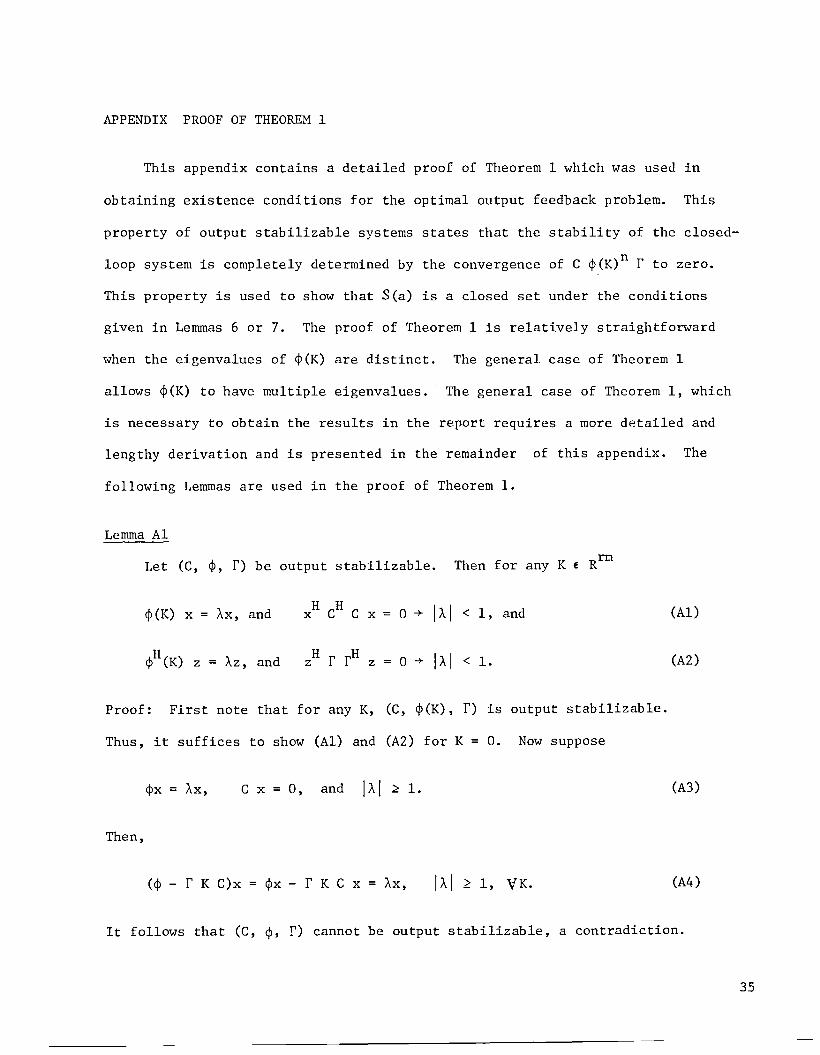
APPENDIX PROOF OF THEOREM 1

This appendix contains a detailed proof of Theorem 1 which was used in

obtaining existence conditions for the optimal output feedback problem. This

property of output stabi1izab1e systems states that the stability of the c1osed­

loop system is completely determined by the convergence of C ¢(K)n f to zero.

This property is used to show that Sea) is a closed set under the conditions

given in Lemmas 6 or 7. The proof of Theorem 1 is relatively straightforward

when the eigenvalues of ¢(K) are distinct. The general case of Theorem 1

allows ¢(K) to have multiple eigenvalues. The general case of Theorem 1, which

is necessary to obtain the results in the report requires a more detailed and

lengthy derivation and is presented in the remainder of this appendix. The

following Lemmas are used in the proof of Theorem 1.

Lemma A1

Let (C, ¢, f) be output stabi1izable.rmThen for any K E R

¢(K) x = AX, and (A1)

AZ, and 0-+ II..I < 1. (A2)

Proof: First note that for any K, (C, ¢(K), f) is output stabi1izab1e.

Thus, it suffices to show (A1) and (A2) for K = O. Now suppose

¢x

Then,

AX, C X 0, and II..I ~ 1. (A3)

(¢ - f K C)x ¢x - f K C x AX, II..I 2: 1, VK. (A4)

It follows that (C, ¢' f) cannot be output stabi1izab1e, a contradiction.

35

Similarly, if

Hcp Z = AZ,

then

0, and IAI 2 1, (AS)

H(CP - f K C) Z Z, IAI 2 1, VK. (A6)

Thus (C, cP, f) is not output stabi1izab1e, a contradiction.

Lemma A2

Let A be an eigenvalue of cP such that

CPX. AX. + xi +1 ' 1 ~ i ~ p, xp+1 O.1 1

Then

n p-1 n-kcP x. k~O bkn A xi +k ' 1 ~ i ~ p, n 2 0,

1

bk n+1 bkn + bk- 1 n' bko = aka' b 0, b 1;-1 n bn

bkn = 0, k > n.

(A7)

(A8)

(A9)

Proof: First note that (A8) holds for n = 0 and n

(A8) holds for an arbitrary n; then

1. Now assume that

,j.,n+1'I' X.

1(A10)

36

p-i An+1- k p-i+1 b An-k'+lk~O bkn xi +k + k'~l k'-l n x i +k '

p-i n+1-k p-i b ,n+1-k'k~O bkn A xi +k + k'~O k'-l n A Xi +k '

p-i +1 kL: (b + b ) ,n -k=O kn k-1 n A Xi +k '

(All)

(A12)

(Al3)

so that (A8) holds for n+l.

Note that the bkn's are the binomial coefficients, xp

is an eigenvector

and x.is a principle vector when i = 1, 2, ... , p. No~ let J be the Jordan1

canonical form of ¢.

X J Z, Z-1

X (A14)

where the columns of X are the principal vectors of ¢. Partition J, X, Z as

J = Z (A15)

a ....••... 1.e.

a

az.e.l 1 a

z.e.2 a 'X.e. 1X.e. ), Z.e. = , J .e.=

P.e.

(A16)

p = max Po,'.e. -L

(A17)

and define the unit step function II as

I1,i ~ j

II ..1J 0, i > j

Lemma A3

C ¢n rJ p-l

Ar:= .Ll k~O Bjk bknJ= J(AlB)

37

where bkn

is given by (A9) , A. , jJ

of ¢, andlj+l-l

-kL Alk Ajl=lj

Bjk0

1, 2, .•. , J are the distinct eigenvalues

A. :f 0;J

(A19)

A. = 0;J

Pl-k

Irk Pl-l i~l Cil i+k Sli '

Proof:

(A2l)

(A22)

since

(A23)

n L Pl Pl nC ¢ r = l~l i~l .Ll Cil · Zf. . ¢ xf.i Sf.iJ= J J

Using Lemma A2,

P -in L Pl Pl f. _n-kSli

C ¢ r = l~l i~l .Ll Cil · Zlj k~O bkn Al xl i+lJ= J

L Pl Pl-i _n-k( Pf.

xl i+l)= lL i~l k~O bkn Al j~l Cilj zl· Sli=1 .1

Noting that

(A2!+ )

(A25)

(A26)

(A27)

38

C ~n r ~ ~l Pl~i Q ,n-k~ = l~l i~l k~O Cil i+l ~li bkn Al (A28)

(A29)

Pt _n-k.L l Ilk . 0. 0 '+k (30' bk 1.. 01= Pt-1 ~ 1 ~1 n ~

(A30)

where

L P -1 (p -kBti)

n-k

t~l t~o f~l at i+k bknXt

L p-l _n-k

t~l k~O Atk bkn At

(A3l)

(A32)

p max Pol~~L ~

(A33)

Now assume that the \t'S have been ordered so that

(A34)

where 1 = tl

< t2

< ••• < tJ

, and the Aj's are distinct. Then (A32) can be

rewritten as

(A35)

which is the desired result.

Lemma A4

Let C ¢n r + o. If IA. I ~ 1, thenJ

o ~ k ~ p-l (A36)

where Aj

' Bjk

are defined in Lemma A3.

Proof: First order the distinct eigenvalues A. of ¢ such thatJ

Suppose that

(A37)

39

(A38)

Since bkn

is a polynomial in n of degree k,

o ~ k ~ p-1 . (A39)

nHence, from the representation in Lemma A3, if C ¢ r + 0, then

Now consider

(A40)

If

p-1k~O [

J,'[;1-- B 'kY J

(A41)

then

p-1 ell pj )k~O j~l Bjkb

k+ 0, p, = A/I A

1 1 , 1 ::: j ::: J 11 ,n J

p-1 ell pj )b

knk~O j~l Bjk b

+ 0, o ~ k ~ p-1p-1 n

Since

(A42)

(A43)

(A44)

bkn + 8

b 1 k p-1p- n

J 11'" B n + 0,wI ' 1 p. .J= J p- J

Using (A46) in (A43)

40

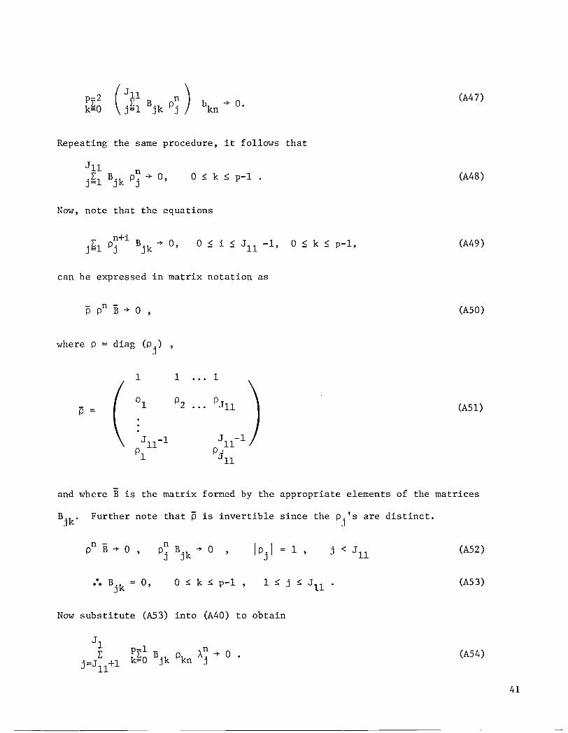
o ::: k ~ p-1 (A45)

(A46)

p-2k~O

(A47)

Repeating the same procedure, it follows that

o ~ k ~ p-1 . (A48)

Now, note that the equations

o ~ i ~ J11 -1, 0 ~ k ~ p-1, (A49)

can be expressed in matrix notation as

(ASO)

where P diag (P.)J

1 1 1

PP1 P2 PJ11

J 11-1 J11

-1P1

PiJ 11

(AS1)

and where B is the matrix formed by the appropriate elements of the matrices

Further note that p is invertible since the P.'s are distinct.J

Ip.1 = 1 ,J

j < J11

(AS2)

.e. Bjk

0, o :s; k :s; p-1 , 1 :s; j :s; J11

. (AS3)

Now substitute (AS3) into (A40) to obtain

(AS4)

41

(J f B. k P~) b

k-+ 0, P. =

j=J +1 J J n J11

(ASS)

Repeating the same procedure as many times as necessary, it follows that

0, o ~ k ~ p-l (AS6)

which is the desired result.

Theorem 1

Let (C, ~, f) be output stabilizable. Then C ~n f -+ 0 if, and only if

p(~) < 1.

Comment: Note that if (C, ~, r) is output stabilizable then (C, ~(K), r)

is output stabilizable where ~(K) is defined in (13). The Theorem is used for

the (C, ~(K), f) system in Lemma 6 but is proved here using (C, ~, f).

Proof: If p(~) < 1, then ~n -+ 0; thus C ~n f -+ O. Now suppose that p(~) ~ 1

and C ~n f -+ 0; let A. be an eigenvalue such that IA.I ~ 1. By Lemma A4,J J

0, o s:: k s:: p-l . (AS7)

,k. BI\J jk

Pl-ki~l (Xl i+k Sli -TIk PI-l 0, o ~ k ::; p-l (ASS)

Now let lj+l = lj + q + 1, q ~ 0; i.e., A. corresponds to q + 1 Jordan forms.J

It is important to note the implications of Lemma Al

to q + 1 linearly independent eigenvectors, namely

o s:: i s:: q} be a set of linearlyThus, let {x.,1

A. correspondsJ

o s:: i s:: q}.

It follows that

{XI.+i Pl.+l'J J

to the multiple eigenvector case.

independent set of eigenvectors corresponding to the eigenvalue A; i.e.,

~X.1

AX. ,1

o ::; i :$ q (AS9)

42

Then for any non-zero sequence { ai' 0::; i ::; q} of complex numbers, the vector

q

x = i~O a. x.1 1

(A60)

is also an eigenvector of ¢ corresponding to A.

Hence, Lemma Al implies that

Cxq

i~O a. Cx. f. 01 1

(A6l)

whenever IAI ~ 1, provided that (C, ¢, f) is output stabilizable. In other words,

the set of vectors { Cxi ' O::S; i ::s; q } is linearly independent. For the problem

at hand, it follows that the set {al

linearly independent. Similarly, it

is linearly independent.

p , l. ::; l < l'+l = l. + q + I} isl J J J

can be shown that {Sl Pi' lj::; l < lj+l}

Now let Pj = max {Pl' lj ::s; l < lj+l } , and 1 ::s; m ::s; Pj" We will show that

(AS 7) implies

(A62)

using finite induction. First note (A62) holds for m

for k Pj - l.

lj+q Pl-Pj+lSlil~l. i~l al i+p.-l ll_ 1

Pl-l0

p.-J J J

lj+q

al Pl Sll 0l~l. ll_PlJ Pj

1, by evaluating (AS8)

(A63)

(A64)

where the fact that Pi - Pj+l ~ 1 has been used to obtain (A64).

a l Pl's are linearly independent, it follows that

Since the

0; i. e. , Sli 0, 1 s:: i s:: Pl p.+l.J

(A6S)

Now suppose that (A62) holds for an arbitrary value m < p., EvaluatingJ

43

(AS8) for k

Ij;qI=l.

J

1, we obtain

o (A66)

Since (A62) holds for m, the only terms which might not vanish correspond

to 1 < . PI - Pj+m+l. Hence (A66) becomes_ 1

Ij+qSI - 0Igi. o.l p IT-

PI-Pj+m+l p.-m PIJ I J

Since the 0.0 's are linearly independent,0{. PI

(A67)

So - IT_o{. PI-PJ.+m+l p.-m PI

J

0, I . .:::; I .:::; I. + qJ J

(A68)

1 .:::; i = PI - Pj

+ m + 1; (A69)

so that (A62) must hold for m + 1, and by induction for 1 .:::; m .:::; P.,J

However, if (A62) holds for m Pj

, then

(A70)

which, by Lemma 1, implies that (C, ¢, f) is not output stabilizable, a con-

tradication. Thus, we must have p(¢) < 1 which concludes the proof.

Finally, an inequality that is used throughout the paper is given in Lemma

AS for completeness.

Lemma AS

Let PI' P2, Wbe non-negative definite (and Hermitian) matrices such that

44

tr {PI W} ~ 0 (A7l)

Proof: Since W ~ 0, let

(An)

tr {PI W} = tr {wHPI w} ~ tr {wH

P2 w} ~ o.

Note that whereas PI W need not be non-negative definite, its trace is

non-negative.

45

kv

Roll Rate, *1 1.0p , --~ -k ~-----~~~T=-I~S:-+:-'-I--;.0"I---~

(Deg/Sec) ~---~

Roll Angle,

*<P,(Deg) -k

* *Phic, Aileron

kS1 k

7<Pc' k

3-k6

SCommand,

(Deg) °AC'(Deg)

FIGURE 1 LATERAL-DIRECTIONAL INNER-LOOP BLOCK DIAGRAMS

Yaw Rate, kg T S ~

("Deg/Sec--)---':~T--3C;s:-';-+-'-l~. on+----.:~::T-3~S-:~11.AO t---~ ~I-kll t-----':.,t

Rudder Command,

°RC'(Deg)

FIGURE 1 LATERAL-DIRECTIONAL INNER-LOOP BLOCK DIAGRAMS (CONCLUDED)

47

TABLE 1 EFFECTS OF CHANGING NOISE COVARIANCE MATRICES§~I

Design Gain Matrix EigenvaluesParameters lIu' = [M M ] A A A

lIi' = [lI1/1~ lIy;Clly ] lIy lIlj! lIr Spiral Dutch Roll Roll llcP !:'r, M !:'pwo a

Outer-loop 0.0 0.0 -0.279 -1.06 -0.94±jO.80 -3.67 -5.0 (-6. 3±j .17) -22.4Open 0Inner-loopClosed

ObservationNoise:

01/1 = 0.1 -0.98 -0.016 -0.061 (-0.32±jO.26) -0.171 -0.436 -0.95±j1.3 -2.85 -5.0 (-6.2±j2.0) -22.40 = 3.05 1.31 0.017 0.067o~ = 3.05

Y

ObservationNoise:

0lj! = 0.32 -0.90 -0.015 -0.064 (-0.32±jO.27) -0.155 -0.446 -0.95±j1.2 -2.86 -5.0 (-6.2±j2.0) -22.40 = 2.16 1.15 0.016 0.079o~ = 0.67

Y

ObservationNoise as Above -0.073 -0.0046 -0.036 (-0.059±j.014) -0.243 -0.914 -0.89±jO.92 -3.95 -5.0 (-6. 2±j 1. 7) -22.4Using Gusts & 0.218 0.0049 0.029Inner-loopMeasurementNoise Only

§Angles-deg, Angular Rates-deg/sec, Velocity-m/sec, Gusts-m/sec, Position-m

~IThe equivalent continuous-time closed-loop eigenvalues are obtained by applying first the log of a matrixto the discrete closed-loop plant then finding the eigenvalues of the resulting matrix.

*TABLE 2 DIAGONAL ELEMENTS OF DESIGNED MATRICES

R - Control Weighting

r~ ~ = 1.0c c

Q - State Weighting

LO

qljJljJ '" 0.25, q~~ =- 0.25, qyy

W - Process Noise

0.00093, q ••yy 0.023

0wg = 3.05, 0p = 0.3, o~ = 0.6, or = 0.3

W+ - Additional Process Noise (Initial Condition State Variance)

0v .. 1.5, o~

OA C 1.0, OAr p 1.0, o¢ = 1.0,

30.5,

° = 1.0r wo

*Angles-deg, Angular Rates-deg/sec, Velocity-m/sec, Gusts-m/sec, Position-m

TABLE 3 ALGORITHM COMPARISONS

Minimization Algorithm I Algorithm II Algorithm IIITechnique (Algorithm III with a = 1.0) (Davidon- (Section V)

Fletcher-Powell)Test 1 :Initial Valuefor J(K ) 179.048 179.048 179.048

0 (a=l.O to start)No. of LyapunovType EquationsSolved 4 122 88

Final Valuefor J(K) --- 176.740 173.605

Diverged Algorithm Prematurely Converged-FinalTerminated Because of a = 0.75Poor Convergence

Test 2:Initial Valuefor J(K ) 173.643 173.643 173.643

0(a=l. 0 to start)

No. of LyapunovType EquationsSolved 4 80 24

Final Valuefor J(K) --- 173.606 173.606

Diverged Converged Converged-Finala = 0.75

49

1. Report No. I2. Government Acceuion No. 3. Recipient's ~tlIlog No.

NASA CR-3828... Title ~nd Subtitle 5. Report Date

INVESTIGATION, DEVELOPHENT, AND APPLICATION OF OPTIMAL August 1984OUTPUT FEEDBACK THEORY. Volume I--A Convergent Algorithm 6. Performing Organization Codefor the Stochastic Infinite-Time Discrete Optimal OutputFeedback Problem

8. Performing Organization Report No.

7. Author(s) FR 683101Nesim Halyo and John R. Broussard

10. W()(k Unit No.

9. Perf()(ming Organization Name and Address

Information & Control Systems, Incorporated 11. Contract or Grant No.

28 Research Drive NASl-15759Hampton, VA 23666

13. Type of Report and Period Covered

12. Sponwring Agency Name and Address Contractor Report

National Aeronautics and Space Administration 14. Spomoring Agency Code

Washington, DC 20546 534-04-13-54.-

15. Supplement~ry Notes

NASA Langley Technical Honitor: Richard M. HueschenFinal Report

16. Abstract

This report considers the stochastic, infinite-time, discrete output feedbackproblem for time-invariant linear systems. Two sets of sufficient conditions forthe existence of a stable, globally optimal solution are presented. An expressionfor the total change in the cost function due to a change in the feedback gain isobtained. This expression is used to show that a sequence of gains can be obtainedby an algorithm, so that the corresponding cost sequence is monotonically decreasingand the corresponding sequence of the cost gradients converges to zero. The algo-rithm is guaranteed to obtain a critical point of the cost function. The computa-tional steps necessary to implement the algorithm on a computer are presented. Theresults are applied to a digital outer-loop flight control problem. The numericalresults for this 13th order problem indicate a rate of convergence considerablyfaster than two other algorithms used for comparison when they converge.

17. Key Words (Suggested by Auth()((sll 18. Distribution Statement

Optimal Control - Theory Unclassified - Unlimited

Optimal Control - ApplicationOutput Feedback

Subject Category 08Numerical Algorithms

19. Security OalSif. (of this report) 20. Security Clanif. (of this pagel 21. No. of P~ 22. Price

Unclassified Unclassified 55 A04

'-105 FOf sale by the National Technical InfOfmation Service. Springfield, Virginia 22161 NASA-Langley. 1984

National Aeronautics andSpace Administration

Washington, D.C.20546Official Business

Penalty for Private Use, $300

THIRO-eLASS BULK RATE Postage and Fees Paid (tJNational Aeronautics and ~Space AdministrationNASA-451 =

NI\SI\ POSTMASTER: If Undeliverable (Section I 58Postal Manual) Do Not Return